Development and evaluation of CO₂ transport in MPAS-A v6.3

Chemistry transport models (CTMs) play an important role in understanding fluxes and atmospheric distribution of carbon dioxide (CO₂). They have been widely used for modeling CO₂ transport through forward simulations and inferring fluxes through inversion systems. With the increasing availability of high-resolution observations, it has been become possible to estimate CO₂ fluxes at higher spatial resolution. In this work, we implemented CO₂ transport in the Model for Prediction Across Scales – Atmosphere (MPAS-A). The objective is to use the variable-resolution capability of MPAS-A to enable a high-resolution CO₂ simulation in a limited region with a global model. Treating CO₂ as an inert tracer, we implemented in MPAS-A (v6.3) the CO₂ transport processes, including advection, vertical mixing by boundary layer scheme, and convective transport. We first evaluated the newly implemented model's tracer mass conservation and then its CO₂ simulation accuracy. A 1-year (2014) MPAS-A simulation is evaluated at the global scale using CO₂ measurements from 50 near-surface stations and 18 Total Carbon Column Observing Network (TCCON) stations. The simulation is also compared with two global models: National Oceanic and Atmospheric Administration (NOAA) CarbonTracker v2019 (CT2019) and European Centre for Medium-Range Weather Forecasts (ECMWF) Integrated Forecasting System (IFS). A second set of simulation (2016–2018) is used to evaluate MPAS-A at regional scale using Atmospheric Carbon and Transport – America (ACT-America) aircraft CO₂ measurements over the eastern United States. This simulation is also compared with CT2019 and a 27 km WRF-Chem simulation. The global-scale evaluations show that MPAS-A is capable of representing the spatial and temporal CO₂ variation with a comparable level of accuracy as IFS of similar horizontal resolution. The regional-scale evaluations show that MPAS-A is capable of representing the observed atmospheric CO₂ spatial structures related to the midlatitude synoptic weather system, including the warm versus cold sector distinction, boundary layer to free troposphere difference, and frontal boundary CO₂ enhancement. MPAS-A's performance in representing these CO₂ spatial structures is comparable to the global model CT2019 and regional model WRF-Chem.

1 Introduction

Carbon dioxide (CO₂) is the most important greenhouse gas, and our knowledge about its sources and sinks still has large gaps. Inversion systems are tools for inferring surface CO₂ fluxes based on observations and chemistry transport models (CTMs). Two types of CTMs are commonly used: global models and regional models. Global models are commonly used for inferring CO₂ fluxes at coarse spatial scales (Patra et al., 2008; Schuh et al., 2019; Jacobson et al., 2007, 2020). With the fast increasing number of atmospheric CO₂ observations, including those acquired by ground-based, airborne, and satellite instruments, regional inversion systems have been developed and applied to estimate carbon fluxes at higher resolution (Gerbig et al., 2009; Pillai et al., 2012; Lauvaux et al., 2012; Hu et al., 2019; Zheng et al., 2018, 2019).

A major challenge of atmospheric CO₂ inversion modeling is how to partition the model–data mismatch (MDM) among the transport model error, observation error, and prior flux error (Baker et al., 2006). In the Bayesian inversion framework, the error covariance matrix R is commonly used to represent the combined error of transport model and observations. While it is important to correctly represent the transport model error in an inversion system, it is also important to reduce the error in order to estimate the fluxes with less uncertainty. One approach to reduce the transport model error is to increase the horizontal resolution of a simulation. For instance, Feng et al. (2016) found high-resolution WRF-Chem simulation improved CO₂ model–data comparison because of better resolved planetary boundary layer (PBL) and better representation of spatial variability of CO₂ fluxes. In a recent study, Agusti-Panareda et al. (2019) investigated the impacts of transport model's horizontal resolutions on simulated CO₂ accuracy, and they found that CO₂ variability is generally better represented by higher-resolution simulations.

Global high-resolution CO₂ simulations require large computational resources. Regional (limited-area) models, which have lower computational cost than their global model counterpart at the same horizontal resolution, are often used for high-resolution CO₂ transport (Feng et al., 2016; Diaz-Isaac et al., 2019, 2018) and inverse modeling (Sarrat et al., 2007; Gerbig et al., 2008; Lauvaux et al., 2012; Zheng et al., 2019). However, a regional model requires CO₂ transported from outside its model domain to be prescribed. For a CO₂ inversion system, having lateral boundaries increases the size of the control vector to be optimized (Rayner et al., 2019). A number of approaches have been applied to the CO₂ lateral boundary problem, such as assuming the boundary inflow is perfectly known (Gockede et al., 2010), correcting the lateral boundary condition using observation prior to inversion (Lauvaux et al., 2012; Schuh et al., 2013), or jointly optimizing flux and lateral boundary condition (Zheng et al., 2018). When the CO₂ lateral boundary is optimized, an inversion system adjusts its CO₂ fields at the boundary prescribed by a parent global model in addition to adjusting surface fluxes. This could be problematic for inversion systems that use satellite-derived column-averaged CO₂ measurements (XCO₂) because model–data mismatches in the free troposphere (FT) are often originated from outside a regional model's limited-area domain (Feng et al., 2019; Lauvaux and Davis, 2014).

The objective of the present paper is to provide an alternative high-resolution CO₂ transport modeling approach to regional transport models. This approach is to use a global variable-resolution model which allows for local grid refinement that enables high-resolution simulation over an interested region without incurring the prohibitively high computational cost or the lateral boundary condition. Variable resolution through local grid refinement has been widely used in numerical weather prediction (NWP) models, such as the Model for Prediction Across Scales – Atmosphere (MPAS-A) (Skamarock et al., 2012), Ocean–Land–Atmosphere Model (OLAM) (Walko and Avissar, 2008a, b), Energy Exascale Earth System Model (E3SM) (Golaz et al., 2019), and Finite-Volume Cubed-Sphere model (FV3) (Putman and Lin, 2007). One benefit of local mesh refinement is enabling regional high-resolution modeling without incurring the lateral boundary condition and its associated problems, such as solution mismatches between the driving global model and the evolving regional model (Davies, 2014). MPAS-A is a fully compressible non-hydrostatic global atmospheric model which uses finite-volume numeric solver discretized on a centroidal Voronoi mesh with C-grid staggering of its prognostic variables (Skamarock et al., 2012; Thuburn, 2007; Ringler et al., 2010). The centroidal Voronoi mesh allows for local refinement and a variable-resolution horizontal mesh which can be gradually changed from coarse to fine resolutions (Skamarock et al., 2012; Ringler et al., 2008).

To enable CO₂ transport modeling, we implemented atmospheric CO₂ transport processes, including advection, vertical mixing by PBL scheme, and convective transport in MPAS-A v6.3. Because the CO₂ transport processes are fully integrated into the model's meteorological time steps, the resulting MPAS-A CO₂ is an online CTM. We used the newly developed model to conduct two sets of simulations over a 60–15 km variable-resolution global domain. Then the simulation results are evaluated using an extensive set of airborne observations over the eastern United States and near-surface observations from surface and tower stations across the globe. The simulation accuracy of MPAS-A is compared with three established CO₂ modeling systems based on the same observational data: WRF-Chem (Skamarock et al., 2008; Feng et al., 2019), CarbonTracker (v2019, CT2019 hereafter) (Jacobson et al., 2020), and the European Centre for Medium-Range Weather Forecasts (ECMWF) Integrated Forecasting System (IFS) (Agusti-Panareda et al., 2014, 2019).

2 Implementation of CO₂ transport in MPAS-A

This section describes the major modifications to MPAS-A that we made to implement CO₂ tracer transport. We represent CO₂ by its dry-air mixing ratio ($q_{{\mathrm{co}}_{\mathrm{2}}}$) and model its atmospheric transport by adding its continuity equation in MPAS-A following Eq. (7) of Skamarock et al. (2012):

$$\begin{array}{}\text{(1)}& {\displaystyle \frac{\partial \left(\stackrel{\mathrm{̃}}{\mathit{\rho }}{q}_{{\mathrm{co}}_{\mathrm{2}}}\right)}{\partial t}}=-(\mathrm{\nabla }\cdot \stackrel{\mathrm{̃}}{\mathit{\rho }}{q}_{{\mathrm{co}}_{\mathrm{2}}}\mathit{V}{)}_{\mathit{\zeta }}+F_{\mathrm{bl}}+F_{\mathrm{cu}},\end{array}$$

where $\stackrel{\mathrm{̃}}{\mathit{\rho }}={\mathit{\rho }}_{\mathrm{d}}/(\partial \mathit{\zeta }/\partial z)$, ρ_d is dry-air density, ζ is the vertical coordinate, z is geometric height, t is time, and $\mathit{V}=(u,v,w)$ is the velocity vector (u, v, and w are the zonal, meridional, and vertical wind, respectively). The left-hand side of the equation is the total CO₂ time tendency ($\partial \left(\stackrel{\mathrm{̃}}{\mathit{\rho }}{q}_{{\mathrm{co}}_{\mathrm{2}}}\right)/\partial t$), and the first, second, and third terms on the right-hand side represent the contributions from advection, vertical mixing, and convective transport, respectively. CO₂ tendency from advection is modeled in flux form (Sect. 2.1), while tendency from vertical mixing (F_bl) and convective transport (F_cu) are modeled in an uncoupled form ($\partial q_{{\mathrm{co}}_{\mathrm{2}}}/\partial t)$, which are coupled to $\stackrel{\mathrm{̃}}{\mathit{\rho }}$ before being added to the total tendency. We choose to implement CO₂ vertical mixing in the Yonsei University (YSU) PBL scheme (Hong et al., 2006), and CO₂ convective transport in Kain–Fritsch (KF) scheme (Kain, 2004) because they are widely used in CTMs and have been validated using observations (Borge et al., 2008; Hu et al., 2010; Kretschmer et al., 2012; Polavarapu et al., 2016). Details of the three terms on the right-hand side of Eq. (1) are described in the following sections. We note that because the monotonicity constraint in the third-order scalar horizontal advection scheme (Skamarock and Gassmann, 2011) introduces dissipation, MPAS-A does not use any explicit horizontal diffusion for scalar. Accordingly, we did not include horizontal diffusion for CO₂.

2.1 CO₂ advection

Advection is the most significant component of CO₂ atmospheric transport. Following the example of other scalars in MPAS-A (Skamarock and Gassmann, 2011), we model CO₂ advection as

$$\begin{array}{}\text{(2)}& \begin{array}{rl}(\mathrm{\nabla }\cdot \stackrel{\mathrm{̃}}{\mathit{\rho }}{q}_{{\mathrm{co}}_{\mathrm{2}}}\mathit{V}{)}_{\mathit{\zeta }}& ={\left[{\displaystyle \frac{\partial \left(\stackrel{\mathrm{̃}}{\mathit{\rho }}u{q}_{{\mathrm{co}}_{\mathrm{2}}}\right)}{\partial x}}+{\displaystyle \frac{\partial \left(\stackrel{\mathrm{̃}}{\mathit{\rho }}v{q}_{{\mathrm{co}}_{\mathrm{2}}}\right)}{\partial y}}\right]}_{\mathit{\zeta }}\\ & +{\displaystyle \frac{\partial \left(\stackrel{\mathrm{̃}}{\mathit{\rho }}w{q}_{{\mathrm{co}}_{\mathrm{2}}}\right)}{\partial \mathit{\zeta }}}.\end{array}\end{array}$$

The first item on the right-hand side enclosed in the square bracket is the CO₂ horizontal flux divergence, and second item is the vertical flux divergence. The horizontal flux divergence is transformed via the divergence theorem into an integral of flux over each control volume, which is modeled as

$$\begin{array}{}\text{(3)}& {\left[{\displaystyle \frac{\partial \left(\stackrel{\mathrm{̃}}{\mathit{\rho }}u{q}_{{\mathrm{co}}_{\mathrm{2}}}\right)}{\partial x}}+{\displaystyle \frac{\partial \left(\stackrel{\mathrm{̃}}{\mathit{\rho }}v{q}_{{\mathrm{co}}_{\mathrm{2}}}\right)}{\partial y}}\right]}_{\mathit{\zeta }}={\displaystyle \frac{\mathrm{1}}{A_i}}\sum _e^{n_{\mathrm{e}}}{l}_{\mathrm{e}}{F}_{\mathrm{e}}({\mathit{V}}_{\mathrm{H}},\stackrel{\mathrm{̃}}{\mathit{\rho }}{q}_{{\mathrm{co}}_{\mathrm{2}}}),\end{array}$$

where e indexes the edges of a cell and n_e represents the number of edges the cell has, l_e is the length of an edge, A_i is the cell's areal size, $F_{\mathrm{e}}({\mathbf{v}}_{\mathrm{H}},\stackrel{\mathrm{̃}}{\mathit{\rho }}{q}_{{\mathrm{co}}_{\mathrm{2}}})$ is the instantaneous horizontal CO₂ flux that crosses the cell edge e, and ${\mathit{V}}_{\mathrm{H}}=(u,v)$ is the horizontal wind vector. The details of MPAS-A instantaneous horizontal flux calculation can found in Skamarock and Gassmann (2011). The vertical CO₂ flux divergence in Eq. (2) is calculated using the finite difference:

$$\begin{array}{}\text{(4)}& {\displaystyle \frac{\partial \left(\stackrel{\mathrm{̃}}{\mathit{\rho }}w{q}_{{\mathrm{co}}_{\mathrm{2}}}\right)}{\partial \mathit{\zeta }}}={\displaystyle \frac{\mathrm{1}}{\mathrm{\Delta }\mathit{\zeta }}}\left[F\right(w,\stackrel{\mathrm{̃}}{\mathit{\rho }}{q}_{{\mathrm{co}}_{\mathrm{2}}}{)}_{k+\frac{\mathrm{1}}{\mathrm{2}}}-F(w,\stackrel{\mathrm{̃}}{\mathit{\rho }}{q}_{{\mathrm{co}}_{\mathrm{2}}}{)}_{k-\frac{\mathrm{1}}{\mathrm{2}}}],\end{array}$$

where $F(w,\stackrel{\mathrm{̃}}{\mathit{\rho }}{q}_{{\mathrm{co}}_{\mathrm{2}}})$ is the vertical CO₂ flux that crosses a cell's vertical face, and k indexes the vertical coordinate.

2.2 CO₂ vertical mixing

Like in WRF (Skamarock et al., 2008), a PBL parameterization in MPAS-A treats the vertical mixing of momentum and scalars not only in the boundary layer (BL) but in the entire atmospheric column. The YSU scheme (Hong et al., 2006) is one of the PBL schemes available in MPAS-A v6.3. The present YSU scheme treats vertical mixing of momentum, potential temperature, and water species but not atmospheric tracers. We modified the scheme to treat CO₂ vertical mixing.

In the YSU scheme, after the top of BL is determined, the vertical mixing processes of momentum, potential temperature, and water vapor are treated separately: above the BL, local K-profile approach (Louis, 1979) is used for vertical diffusion of momentum and scalars (Noh et al., 2003; Hong et al., 2006). Within the BL, an entrainment flux at the inversion layer is included for momentum and scalar diffusion. In addition, a countergradient mixing term is included for the diffusion of momentum and potential temperature to account for the convective-driven mixing (γ_c of Eq. 4 in Hong et al., 2006), but this term is not used for water vapor.

Following the treatment of water vapor, we parameterize CO₂ vertical mixing in BL as

$$\begin{array}{}\text{(5)}& {\displaystyle \frac{\partial q_{{\mathrm{co}}_{\mathrm{2}}}}{\partial t}}={\displaystyle \frac{\partial }{\partial z}}[K_{\mathrm{h}}\left({\displaystyle \frac{\partial q_{{\mathrm{co}}_{\mathrm{2}}}}{\partial z}}\right)-\stackrel{\mathrm{‾}}{(w^{\prime }{q}_{{\mathrm{co}}_{\mathrm{2}}}^{\prime }{)}_{\mathrm{h}}}{\left({\displaystyle \frac{z}{h}}\right)}^{\mathrm{3}}],\end{array}$$

where z is the vertical distance to surface, h is BL top height, K_h is vertical eddy diffusivity. Note that this formulation does not include a countergradient mixing term following the treatment of water vapor in the original YSU scheme (Hong et al., 2006). The second term in the square brackets of Eq. (5) represents the contribution from CO₂ entrainment flux at the inversion layer, which is parameterized as

$$\begin{array}{}\text{(6)}& \stackrel{\mathrm{‾}}{(w^{\prime }{q}_{{\mathrm{co}}_{\mathrm{2}}}^{\prime }{)}_{\mathrm{h}}}=w_{\mathrm{e}}\mathrm{\Delta }{q}_{{\mathrm{co}}_{\mathrm{2}}}{|}_{\mathrm{h}},\end{array}$$

where $\mathrm{\Delta }{q}_{{\mathrm{co}}_{\mathrm{2}}}{|}_{\mathrm{h}}$ is the CO₂ mixing ratio difference across the inversion layer, and w_e is the entrainment rate at the inversion layer calculated by Eq. (A11) of Hong et al. (2006). Above BL top, vertical mixing of CO₂ is parameterized as

$$\begin{array}{}\text{(7)}& {\displaystyle \frac{\partial q_{{\mathrm{co}}_{\mathrm{2}}}}{\partial t}}={\displaystyle \frac{\partial }{\partial z}}\left[K_{\mathrm{h}}\left({\displaystyle \frac{\partial q_{{\mathrm{co}}_{\mathrm{2}}}}{\partial z}}\right)\right].\end{array}$$

We use the same value for CO₂ vertical diffusivity as water vapor. The details of K_h calculation can be found in the Appendix of Hong et al. (2006), and its value is limited between 0.01 and 1000 m² s⁻¹ to prevent too-weak or too-strong vertical mixing. The term $\partial q_{{\mathrm{co}}_{\mathrm{2}}}/\partial t$ from Eq. (5) is coupled with dry-air density before being applied to the continuity equation (Eq. 1).

2.3 CO₂ convective transport

For convective transport, we modified the KF scheme (Kain, 2004) to include the CO₂ treatment. KF is a mass-flux convection scheme which rearranges mass in an air column using convective updrafts, downdrafts, and environmental mass fluxes. Both the updraft and downdraft entrain from and detrain to the environment, thus altering the vertical profile of an air column's thermodynamic properties. We added the CO₂ convective transport as

$$\begin{array}{}\text{(8)}& \begin{array}{rl}{\displaystyle \frac{\partial q_{{\mathrm{co}}_{\mathrm{2}}}}{\partial t}}& ={\displaystyle \frac{(M_{\mathrm{u}}+M_{\mathrm{d}})}{\mathit{\rho }A}}{\displaystyle \frac{\partial q_{{\mathrm{co}}_{\mathrm{2}}}}{\partial z}}+{\displaystyle \frac{M_{\mathrm{ud}}}{M}}(q_{{\mathrm{co}}_{\mathrm{2}}}^{\mathrm{u}}-q_{{\mathrm{co}}_{\mathrm{2}}})\\ & +{\displaystyle \frac{M_{\mathrm{dd}}}{M}}(q_{{\mathrm{co}}_{\mathrm{2}}}^{\mathrm{d}}-q_{{\mathrm{co}}_{\mathrm{2}}}),\end{array}\end{array}$$

where $q_{{\mathrm{co}}_{\mathrm{2}}}$, $q_{{\mathrm{co}}_{\mathrm{2}}}^{\mathrm{u}}$, and $q_{{\mathrm{co}}_{\mathrm{2}}}^{\mathrm{d}}$ are the CO₂ mixing ratio in the environment, updraft, and downdraft, respectively, M_u and M_d are the updraft and downdraft mass, respectively, ρ is the environment air density, A is the horizontal area of a cell, M=ρAδz is the mass of environmental air in a grid box, and M_ud and M_dd are the detrainment from the updraft and downdraft, respectively.

In the KF scheme, the updraft and downdraft mass and the rates for the entrainment and detrainment are determined by a steady-state plume model and a convective available potential energy (CAPE) closure assumption: 90 % of the existing CAPE should be removed by the convection parameterization (Kain and Fritsch, 1990; Fritsch and Chappell, 1980; Kain, 2004). Because the calculation of the updraft and downdraft mass fluxes is related to a cell's horizontal area, the KF scheme may behave differently in different areas of MPAS-A's variable-resolution grid. The updraft source layers are determined by a search from the model's lowest vertical level for a group of consecutive layers that is buoyant and at least 50 hPa deep (Kain, 2004). The initial value of CO₂ mixing ratio in the updraft is modeled as a pressure-weighted average of the source layers:

$$\begin{array}{}\text{(9)}& q_{{\mathrm{co}}_{\mathrm{2}}}^{\mathrm{u}}=\sum _k{\displaystyle \frac{\mathit{\delta }{q}_{{\mathrm{co}}_{\mathrm{2}},k}\mathit{\delta }{p}_k}{\mathit{\delta }{p}_k}},\end{array}$$

where δp_k is layer's pressure depth, and $q_{{\mathrm{co}}_{\mathrm{2}},k}$ is the layer's CO₂ mixing ratio. The CO₂ mixing ratio of the updraft is modified by the entrainment of the environmental air through its ascent from its starting level to the cloud top.

$$\begin{array}{}\text{(10)}& q_{{\mathrm{co}}_{\mathrm{2}}}^{\mathrm{u}}={\displaystyle \frac{q_{{\mathrm{co}}_{\mathrm{2}}}^{\mathrm{u}}{M}_{\mathrm{u}}+q_{{\mathrm{co}}_{\mathrm{2}}}{M}_{\mathrm{ue}}}{M_{\mathrm{u}}+M_{\mathrm{ue}}}},\end{array}$$

where M_ue is the updraft entrainment. The initial CO₂ mixing ratio of a downdraft ($q_{\mathrm{co}\mathrm{2}}^{\mathrm{d}}$) is the same as that of the environment (q_co2) at the downdraft starting level and it is modified by entrainment through the downdraft descent:

$$\begin{array}{}\text{(11)}& q_{{\mathrm{co}}_{\mathrm{2}}}^{\mathrm{d}}={\displaystyle \frac{q_{{\mathrm{co}}_{\mathrm{2}}}^{\mathrm{d}}{M}_{\mathrm{d}}+q_{{\mathrm{co}}_{\mathrm{2}}}{M}_{\mathrm{de}}}{M_{\mathrm{d}}+M_{\mathrm{de}}}},\end{array}$$

where M_de is the downdraft entrainment.

3 Model evaluation

In this section, we evaluate the newly developed MPAS-A CO₂ transport model by comparing its simulation results with observations and other models. After describing the simulation configuration (Sect. 3.1), we assess the model's global mass conservation property (Sect. 3.2). Then we evaluate the model's CO₂ transport accuracy at the global scale using hourly near-surface CO₂ observations from 50 in situ stations and column-averaged CO₂ dry-air mole fraction (XCO₂) measurements from 18 Total Carbon Column Observing Network (TCCON) stations (Sect. 3.3). Finally, we evaluate MPAS-A at the regional scale using high-resolution airborne measurements from the Atmospheric Carbon and Transport (ACT) campaign over the eastern United States (Sect. 3.4). MPAS-A CO₂ transport is also compared with three established CTMs: NOAA CT2019 (Jacobson et al., 2020), ECMWF IFS (Agusti-Panareda et al., 2019), and WRF-Chem (Skamarock et al., 2008). In the following model evaluation, we use root mean square error (RMSE), bias (μ), and random error (SE) as the model accuracy metrics:

$$\begin{array}{}\text{(12)}& {\displaystyle }\text{RMSE}=\sqrt{{\displaystyle \frac{\mathrm{1}}{N}}\sum _{i=\mathrm{1}}^N(m_i-o_i{)}^{\mathrm{2}}}\text{(13)}& {\displaystyle }\mathit{\mu }={\displaystyle \frac{\mathrm{1}}{N}}\sum _{i=\mathrm{1}}^N(m_i-o_i)\text{(14)}& {\displaystyle }\text{SE}=\sqrt{{\displaystyle \frac{\mathrm{1}}{N}}\sum _{i=\mathrm{1}}^N(m_i-o_i-\mathit{\mu }{)}^{\mathrm{2}}},\end{array}$$

where o_i and m_i represent the observed and modeled values, respectively.

For model–data intercomparison, MPAS-A model data need to be interpolated to the observation space. Following Patra et al. (2008), the model is sampled in the horizontal by taking the nearest cell over land. MPAS-A uses a height-based terrain-following vertical coordinate (Skamarock et al., 2012). At a given cell, the height of the kth vertical layer boundary is denoted as $z_k^{\mathrm{h}}$. The height of the layer center is $z_k=\mathrm{0.5}\times (z_k^{\mathrm{h}}+z_{k+\mathrm{1}}^{\mathrm{h}})$. In MPAS-A, horizontal wind fields are defined at the vertical layer boundaries and CO₂ fields are defined at layer centers. For horizontal wind field validations using radiosonde data (Sect. 3.3.1), the column profiles of air pressure and horizontal wind fields defined at layer boundaries are used to interpolate to the measurements' pressure levels. To compare with near-surface CO₂ observations from in situ stations (Sect. 3.3.3) and aircraft observations (Sect. 3.4), model CO₂ defined at layer centers is interpolated to the measurement heights. Vertical interpolation and integration for the comparison with TCCON XCO₂ are described in Sect. 3.3.4. MPAS-A simulation outputs are saved at 1 h intervals. For comparison with radiosonde observations and near-surface CO₂ observations, no temporal interpolations are applied: observations are paired with the closest hourly MPAS-A output. For comparison with aircraft observations, the hourly model outputs that bracket an observation's time stamp are used for the temporal interpolation.

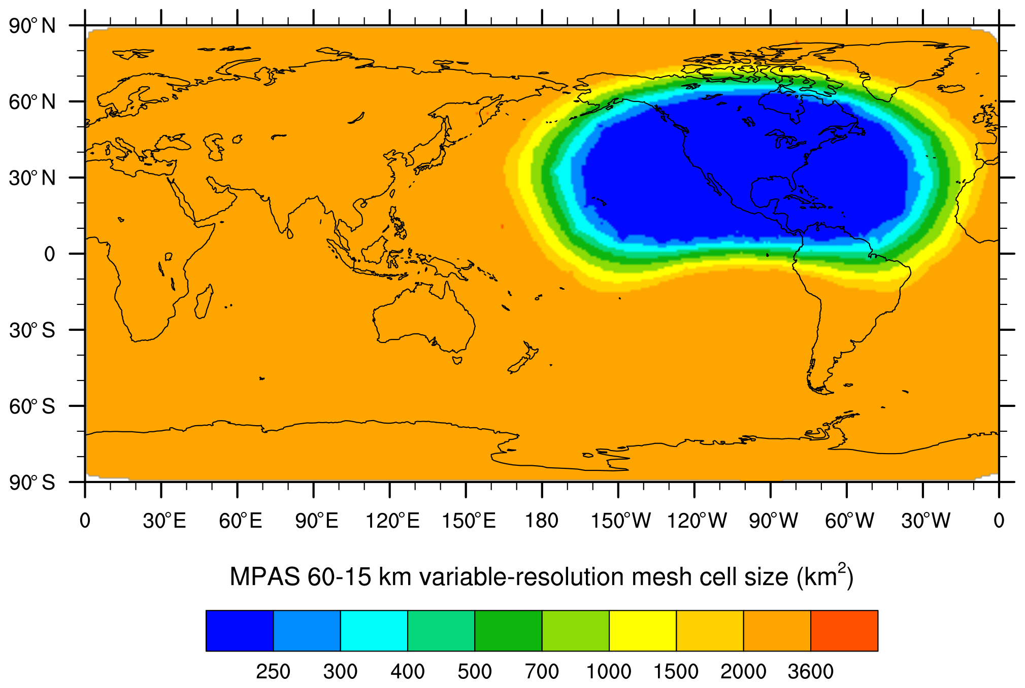
Figure 1 Variable-resolution 60–15 km global domain for MPAS-A CO₂ simulations conducted for model evaluation using aircraft and near-surface CO₂ observations. The highest-resolution (15 km) grid covering the most of North America has a cell size of less than 250 km². The cell sizes (represented by color) gradually increase to about 3600 km² for the rest of the global domain.

3.1 Simulation experiment configuration

For all subsequent simulations, MPAS-A uses a 60–15 km variable-resolution global mesh. Figure 1 shows the cell size (in km²) of the simulation domain, where the highest resolution (15 km) over North America has a cell size smaller than 250 km², which gradually increases to about 3600 km² for the rest of the global domain. In the vertical direction, there are 55 levels spanning from the surface to 30 km above the mean sea level. The model time step is 90 s, which is in accordance with the highest (15 km) horizontal resolution. For physical parameterizations, in addition to the modified YSU PBL (Hong et al., 2004) and Kain–Fritsch cumulus schemes (Kain, 2004) described in Sect. 2, we use RRTMG for longwave and shortwave radiation (Iacono et al., 2008), the Noah land scheme (Chen and Dudhia, 2001), the Monin–Obukhov surface layer scheme, and the WRF single-moment six-class microphysics scheme (Hong and Lim, 2006). Third-order accuracy advection is used for all scalars and the CO₂ tracer. A summary of the physics parameterizations used in the simulations is given in Table 1.

Iacono et al. (2008)Iacono et al. (2008)Hong et al. (2006)Chen and Dudhia (2001)Kain (2004)Hong and Lim (2006)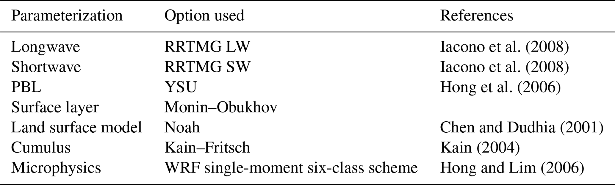

Table 1 MPAS-A CO₂ transport model configuration.

Initial meteorological fields are generated from the ERA-Interim reanalysis (Dee et al., 2011). To keep model meteorological fields close to the reanalysis, MPAS-A meteorological fields are re-initialized using the analysis at 00:00 UTC each day throughout a simulation period. The CO₂ mixing ratio is kept unchanged during the meteorology re-initializations; thus, it is a free-running simulation. This configuration is the same as that used by Agusti-Panareda et al. (2014, 2019) in their IFS global CO₂ simulations. The first CO₂ initial condition for a simulation is from the CT2019 3^∘ × 2^∘ posterior dry-air mole fraction product and surface CO₂ fluxes are prepared by interpolating the CT2019 3-hourly 1^∘ × 1^∘ posterior flux product (Jacobson et al., 2020). The four components of CT2019 fluxes (biosphere, ocean, fossil fuel, and fire) are interpolated to the MPAS-A model grid and ingested at 3 h intervals throughout a simulation.

3.2 CO₂ mass conservation

For CTMs, it is very important to maintain the global CO₂ mass conservation (Agusti-Panareda et al., 2017; Polavarapu et al., 2016). Because meteorological re-initializations introduce changes in dry-air mass, they impact MPAS-A's global CO₂ mass conservation. We first examine MPAS-A's inherent mass conservation property through a simulation without the meteorological re-initializations in Sect. 3.2.1. Then we examine and treat the impacts of the meteorological re-initializations in Sect. 3.2.2.

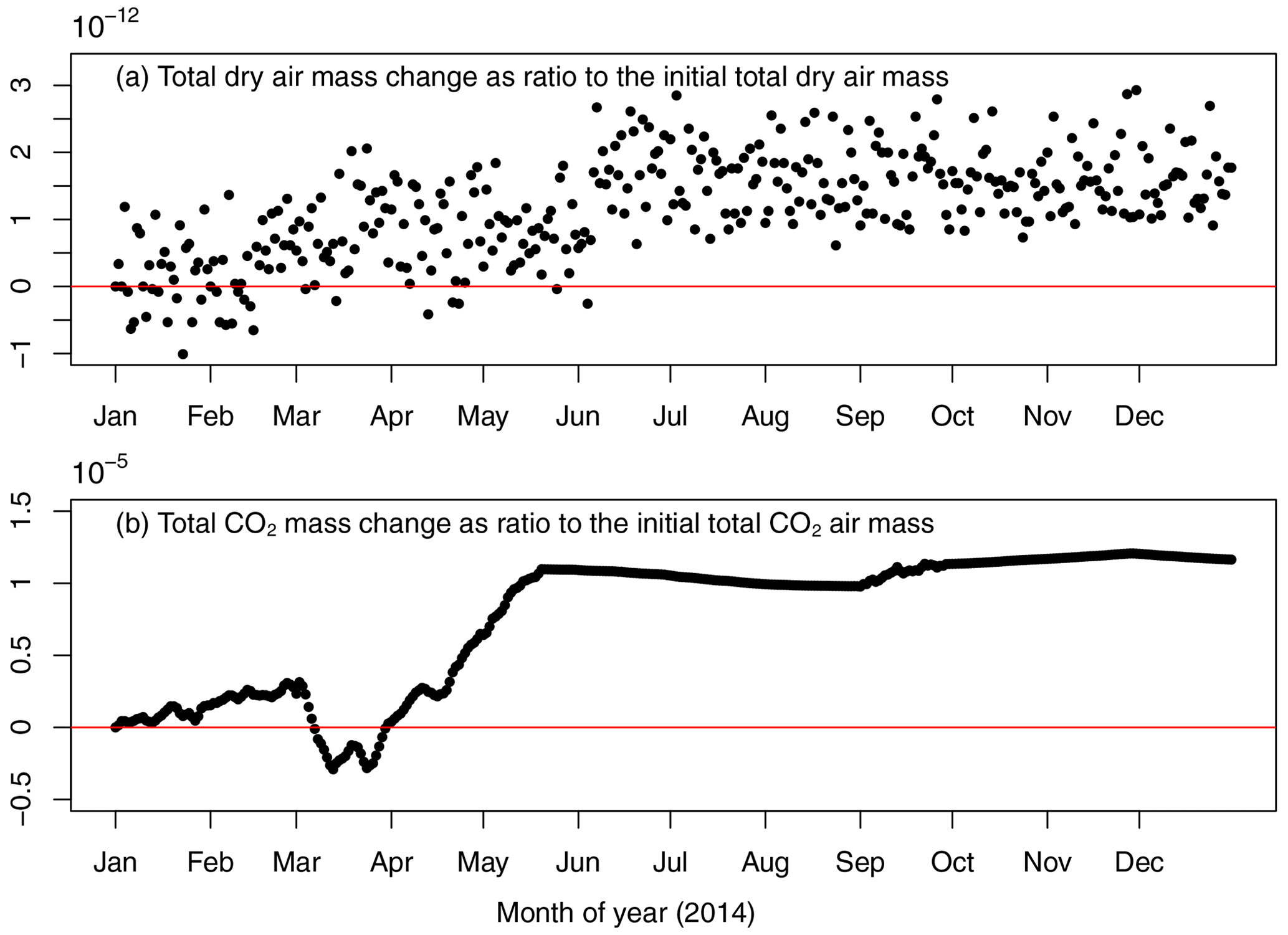
Figure 2 Variation of total dry-air mass (a) and total CO₂ mass (b) as the ratio to their respective starting values during a 1-year continuous MPAS-A simulation without meteorological re-initialization. The x axis represents the days of 2014 and the y axis the ratio of the total mass change to the starting values.

3.2.1 Mass conservation without meteorology re-initialization

To examine MPAS-A's mass conservation property, we conducted a MPAS-A simulation that lasts from 1 January to 31 December 2014. The simulation is initialized with the CT2019 CO₂ mole fraction and is driven with 3-hourly CT2019 surface CO₂ fluxes. Meteorological re-initializations are not applied during the simulation and the model outputs are saved using double precision. MPAS-A's global dry-air mass (M_air) is then calculated at 00:00 UTC each day through the 1-year simulation using Eq. (15):

$$\begin{array}{}\text{(15)}& {\mathrm{M}}_{\mathrm{air}}=\sum _k^L\left(\sum _i^N{A}_i{h}_{i,k}{\mathit{\rho }}_{i,k}\right),\end{array}$$

where subscript i indexes the horizontal cell, subscript k indexes the vertical level, A_i is cell size, h_i,k is cell height, and ρ_i,k is dry-air density (kg m⁻³). After the model's global dry-air mass is calculated at 00:00 UTC each day of the simulation period, its variation is quantified as a ratio $E_{\mathrm{air}}^t=(M_{\mathrm{air}}^t-M_{\mathrm{air}}^{\mathrm{0}})/M_{\mathrm{air}}^{\mathrm{0}}$, where $M_{\mathrm{air}}^{\mathrm{0}}$ and $M_{\mathrm{air}}^t$ are the model's global dry-air mass at the simulation start (00:00 UTC, 1 January 2014) and the current time step, respectively. The top panel of Fig. 2 shows $E_{\mathrm{air}}^t$ at 00:00 UTC of each day through the 1-year simulation period. The figure shows that the maximal magnitude of $E_{\mathrm{air}}^t$ is less than $\mathrm{4}\times {\mathrm{10}}^{-\mathrm{12}}$ during the 1-year simulation. In comparison, the total dry-air mass of ECMWF IFS increases by about 0.01 % of its initial value in a 10 d forecast (Diamantakis and Flemming, 2014). Similarly, the Environment and Climate Change Canada (ECCC) Global Environmental Multiscale (GEM-MACH-GHG) model loses about 0.01 % of its initial total dry-air mass in a 10 d forecast (Polavarapu et al., 2016). MPAS-A has a significantly lower global dry-air mass variation than the two global models because its explicit grid point advection scheme conserves mass (Skamarock and Gassmann, 2011), while the semi-Lagrangian advection scheme used by IFS and GEM-MACH-GHG does not conserves mass (Williamson, 1990). Thus, no mass fixer (Diamantakis and Flemming, 2014; Polavarapu et al., 2016) is used in MPAS-A.

MPAS-A's global CO₂ mass ($M_{{\mathrm{co}}_{\mathrm{2}}}$) is calculated using Eq. (16):

$$\begin{array}{}\text{(16)}& M_{{\mathrm{co}}_{\mathrm{2}}}=\sum _k^L\left(\sum _i^N{A}_i{h}_{i,k}{\mathit{\rho }}_{i,k}{q}_{i,k}\right),\end{array}$$

where q_i,k is the CO₂ dry-air mixing ratio ($\mathrm{kg}/\mathrm{kg}$) and the rest of the terms are the same as in Eq. (15). To assess the global CO₂ mass conservation, $M_{{\mathrm{co}}_{\mathrm{2}}}$ calculated using Eq. (16) is adjusted for the CO₂ mass introduced through the ingestion of the 3-hourly surface CO₂ fluxes. For a 3 h period, total CO₂ mass introduced through the surface CO₂ fluxes is ${\sum }_i^N{A}_i{F}_i\mathrm{\Delta }t$, where F_i is the combined biosphere, ocean, fossil fuel, and fire CO₂ fluxes ($\mathrm{kg}{\mathrm{m}}^{-\mathrm{2}}{\mathrm{s}}^{-\mathrm{1}}$) at a surface cell, A_i is the cell's areal size, N is number of surface cell, and Δt=3 h. After the adjustment, the variation of global mass of CO₂ is quantified as a ratio, $E_{{\mathrm{co}}_{\mathrm{2}}}^t=(M_{{\mathrm{co}}_{\mathrm{2}}}^t-M_{{\mathrm{co}}_{\mathrm{2}}}^{\mathrm{0}})/M_{{\mathrm{co}}_{\mathrm{2}}}^{\mathrm{0}}$, where $M_{{\mathrm{co}}_{\mathrm{2}}}^{\mathrm{0}}$ and $M_{{\mathrm{co}}_{\mathrm{2}}}^t$ are the global CO₂ mass at the initial and current time step, respectively. $E_{{\mathrm{co}}_{\mathrm{2}}}^t$ at 00:00 UTC of each day of the simulation period is shown in the lower panel of Fig. 2. The figure shows that the maximal magnitude of $E_{{\mathrm{co}}_{\mathrm{2}}}^t$ is about 10⁻⁵. This is much higher compared to $E_{\mathrm{air}}^t$ and it is due to the strong gradients caused by surface CO₂ flux which challenge the model's numerical scheme.

3.2.2 CO₂ mass conservation during meteorology re-initialization

When meteorological re-initialization is applied during a simulation, the values of dry-air density in MPAS-A are replaced by values from the initialization files generated from the ERA-Interim reanalysis. In most cases, this will cause dry-air density change which in turn will introduce CO₂ mass change if CO₂ dry-air mixing ratios are kept unchanged during the re-initialization. To assess this possible change in global CO₂ mass, we conducted another 1-year long MPAS-A simulation identical to that used in Sect. 3.2.1, except that meteorological re-initialization was applied at 24 h intervals during the simulation. The variation of global CO₂ mass caused by a meteorological re-initialization is quantified as a ratio $E=(M_{{\mathrm{co}}_{\mathrm{2}}}^{\prime }-M_{{\mathrm{co}}_{\mathrm{2}}})/M_{{\mathrm{co}}_{\mathrm{2}}}$, where $M_{{\mathrm{co}}_{\mathrm{2}}}$ and $M_{{\mathrm{co}}_{\mathrm{2}}}^{\prime }$ are the global CO₂ mass before and after a meteorological re-initialization. The top panel of Fig. 3 shows the value of E at each meteorological re-initialization. The figure indicates that a meteorological re-initialization could cause a change of more than 0.01 % of the global CO₂ mass.

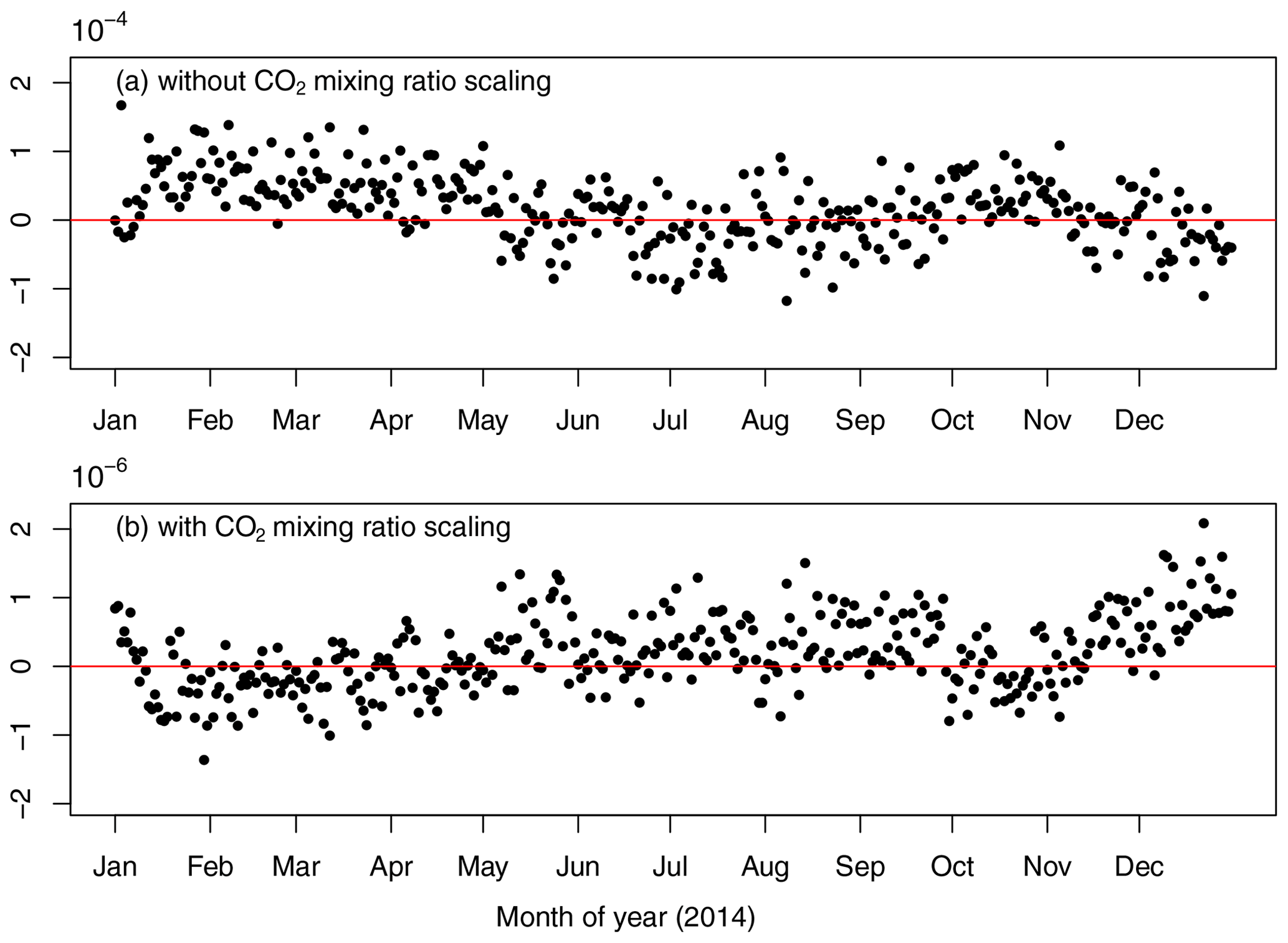
Figure 3 Variation of global CO₂ mass as the ratio to its value prior to a meteorological re-initialization during a 1-year MPAS-A simulation with meteorological re-initializations at 24 h intervals. The top panel is from the simulation without applying CO₂ mixing ratio scaling as described in Sect. 3.2.2, and the bottom panel is from the simulation with the scaling. In each figure, the x axis represents the days of 2014 and the y axis the ratio of global CO₂ mass variation to its value prior to a meteorological re-initialization.

To keep the CO₂ mass conservation after a meteorological re-initialization, we adjust MPAS-A's CO₂ fields by a spatially uniform scaling factor: $q_{i,k}^{\prime }=r\times q_{i,k}$, where q_i,k and $q_{i,k}^{\prime }$ are the CO₂ dry-air mixing ratio, before and after the adjustment, respectively. The scaling factor r is calculated as

$$\begin{array}{}\text{(17)}& r={\displaystyle \frac{{\sum }_k^L\left({\sum }_i^N{A}_i{h}_{i,k}{\mathit{\rho }}_{i,k}{q}_{i,k}\right)}{{\sum }_k^L\left({\sum }_i^N{A}_i{h}_{i,k}{\mathit{\rho }}_{i,k}^{\prime }{q}_{i,k}\right)}},\end{array}$$

where the notations are the same as in Eq. (16) except that ${\mathit{\rho }}_{i,k}^{\prime }$ is the dry-air density after a meteorology re-initialization and ρ_i,k is the value before the re-initialization. To test the effectiveness of this scaling method, the 1-year MPAS-A simulation with meteorological re-initialization was conducted again but this time with the CO₂ dry-air mixing ratio adjustment applied after each meteorological re-initialization. The resulting variation in total CO₂ mass is plotted in the lower panel of Fig. 3. The figure shows the maximal magnitude of the variation caused by a meteorological re-initialization has been reduced from $\sim {\mathrm{10}}^{-\mathrm{4}}$ to $\sim {\mathrm{10}}^{-\mathrm{6}}$ of the global CO₂ mass. Note the different scales in the y axis used in the top and bottom panels of Fig. 3.

An alternative approach to restore mass conservation is to scale the CO₂ mixing ratio at each grid box individually by

$$\begin{array}{}\text{(18)}& q_{i,k}^{\prime }={\displaystyle \frac{{\mathit{\rho }}_{i,k}}{{\mathit{\rho }}_{i,k}^{\prime }}}\times q_{i,k},\end{array}$$

where the notation is the same as that in Eq. (17). This scaling approach can maintain global CO₂ mass conservation as allowed by machine precision but it will introduce artificial spatial variations in CO₂ mixing ratio. In the simulations in the following sections, we chose to use the first scaling approach to avoid the artificial CO₂ mixing ratio variation by accepting the small changes in global CO₂ mass.

3.3 Model evaluation at global scale

In this section, we evaluate the MPAS-A CO2 transport at the global scale. For the model evaluation, MPAS-A was initialized at 00:00 UTC on 1 July 2013 and ran until 31 December 2014. The model configuration for this simulation is as described in Sect. 3.1. With the first 6-month as model spin-up, we use the 1-year simulation of 2014 for the model evaluation. First, MPAS-A simulated horizontal wind fields are evaluated using radiosonde measurements from 457 stations. Then, the model's CO₂ fields are compared with CT2019, near-surface CO₂ measurements from 50 stations, and XCO₂ retrievals from 18 TCCON stations.

3.3.1 Evaluation of horizontal wind fields

Accurate meteorological fields are critical for an accurate CO₂ transport simulation. Before evaluating the simulated CO₂, we evaluate the MPAS-A simulated horizontal wind fields considering their importance in CO₂ advection. We compare MPAS-A simulated horizontal wind fields at 12:00 and 00:00 UTC each day of the simulation period with radiosonde observations from 457 stations located around the globe at four pressure levels: 1000, 850, 500, 850, and 200 hPa. Note that because of the 24-hourly meteorological re-initialization, the 00:00 and 12:00 UTC simulation results are 12 and 24 h forecasts, respectively. The locations of the 457 radiosonde stations are shown in Fig. S1 of the Supplement.

Table 2 Evaluation of MPAS-A simulated horizontal wind using NOAA Integrated Global Radiosonde Archive (IGRA) radiosonde data. Radiosonde data from 457 stations over the globe are used for the evaluation. Wind speed and direction are compared at 00:00 and 12:00 UTC at four pressure levels (1000, 850, 500, and 200 hPa) for each day of the MPAS-A simulation. The number of data samples (N) is smaller at 1000 hPa because some stations are located above that pressure level.

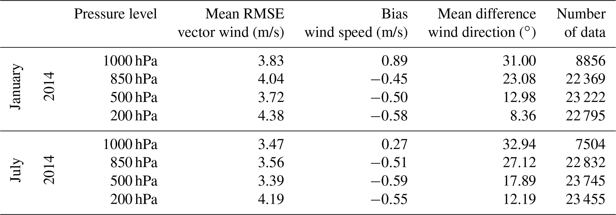
To compare with the similar validation results reported in Agusti-Panareda et al. (2019), the horizontal wind field evaluation results for January and July of 2014 are listed in Table 2. The table shows that while the mean difference in wind direction decreases with altitude, the mean RMSE vector wind generally increases with altitude, which agrees with the IFS validation results (Agusti-Panareda et al., 2019). At the 1000 hPa level, MPAS-A has a slightly lower accuracy than IFS during the same time period. For instance, MPAS-A's mean RMSE vector wind at 1000 hPa is 3.83 m s⁻¹ for January 2014, and IFS results range from 3.2 to 3.75 m s⁻¹ for its 9 and 80 km horizontal resolution simulations. For July 2014, the mean RMSE vector wind at 1000 hPa is 3.47 m s⁻¹ from MPAS-A and 3.0 to 3.6 m s⁻¹ for the IFS 9 and 80 km simulations. At upper level, MPAS-A has a slightly higher accuracy than IFS: at 500 hPa, MPAS-A mean RMSE vector wind is 3.72 and 3.39 m s⁻¹ for January and July 2014, respectively, while IFS results in 4.0–4.1 and 3.5–3.6 m s⁻¹ for the same time period.

Table 3 The statistics of MPAS-A simulated horizontal wind validated at radiosonde stations located in North America. In each cell, the first value is from the 60–15 km variable-resolution grid simulation (labeled as 15 km) and the second is from the 60 km uniform grid simulation (labeled as 60 km). Note that the number of data at 850 and 1000 hPa is different between the two simulations because of the differences in their grids' topography.

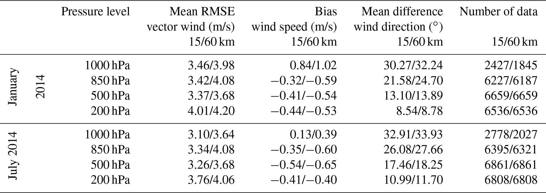
An important finding of Agusti-Panareda et al. (2019) is that higher horizontal resolution generally leads to higher meteorological and CO₂ simulation accuracy. To examine the influence of horizontal resolution on MPAS-A's meteorological simulation accuracy, we conducted an additional set of simulations using the identical configuration except with a global 60 km uniform-resolution grid instead of the 60–15 km variable-resolution grid (Fig. 1). Out of the 475 radiosonde stations, 131 are located in 15 km cells in the 60–15 km variable-resolution simulation. These 131 radiosonde stations are all located at 60 km cells in the 60 km uniform-resolution simulation. In Table 3, we calculated and compared horizontal wind accuracy at these 131 radiosonde stations between the 60 km uniform-resolution simulation (labeled as 60 km) and the 60–15 km variable-resolution simulation (labeled as 15 km). The table shows that the horizontal wind fields at these 131 stations are simulated with considerably higher accuracy on the 15 km grid than its 60 km grid counterpart. For instance, at 1000 hPa, the mean RMSE wind vector for January 2014 is 3.46 and 3.98 m s⁻¹ at the 15 and 60 km grids, respectively. The values are 3.10 and 3.64 m s⁻¹ for July 2014. Table 3 also shows that the difference in the mean RMSE wind vector between the 15 and 60 km grids is larger near the surface at 850 and 1000 hPa than in the middle and upper troposphere (500 and 200 hPa), which is consistent with the findings of Agusti-Panareda et al. (2019). For both January and July at the four pressure levels, the mean RMSE wind vector at the 131 radiosonde stations in MPAS-A's 15 km grid is either similar to or slightly lower than the mean RMSE wind vector of the around 400 stations from the IFS 9 km resolution simulation (Agusti-Panareda et al., 2019).

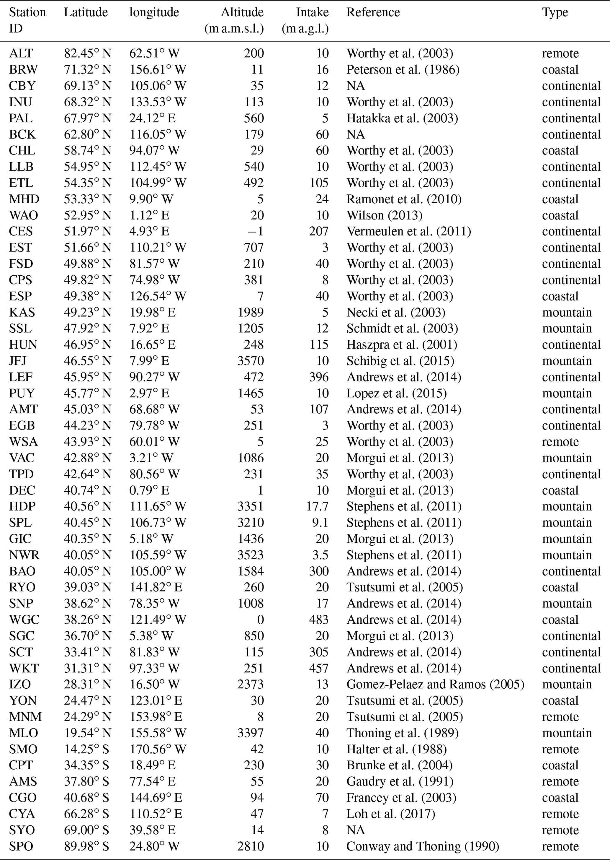
Worthy et al. (2003)Peterson et al. (1986)Worthy et al. (2003)Hatakka et al. (2003)Worthy et al. (2003)Worthy et al. (2003)Worthy et al. (2003)Ramonet et al. (2010)Wilson (2013)Vermeulen et al. (2011)Worthy et al. (2003)Worthy et al. (2003)Worthy et al. (2003)Worthy et al. (2003)Necki et al. (2003)Schmidt et al. (2003)Haszpra et al. (2001)Schibig et al. (2015)Andrews et al. (2014)Lopez et al. (2015)Andrews et al. (2014)Worthy et al. (2003)Worthy et al. (2003)Morgui et al. (2013)Worthy et al. (2003)Morgui et al. (2013)Stephens et al. (2011)Stephens et al. (2011)Morgui et al. (2013)Stephens et al. (2011)Andrews et al. (2014)Tsutsumi et al. (2005)Andrews et al. (2014)Andrews et al. (2014)Morgui et al. (2013)Andrews et al. (2014)Andrews et al. (2014)Gomez-Pelaez and Ramos (2005)Tsutsumi et al. (2005)Tsutsumi et al. (2005)Thoning et al. (1989)Halter et al. (1988)Brunke et al. (2004)Gaudry et al. (1991)Francey et al. (2003)Loh et al. (2017)Conway and Thoning (1990)

Table 4 Continuous in situ stations used for evaluating MPAS-A CO₂ simulation accuracy. NA denotes references that are not available.

3.3.2 Comparison of CO₂ fields with CarbonTracker

Having established that the horizontal wind fields simulated by MPAS-A are sufficiently accurate, the CO₂ fields can be evaluated. Here, we directly compare the simulated XCO₂ by MPAS-A and CT2019 at the grid scale. CT2019 (Jacobson et al., 2020) is an operational carbon data-assimilation system which uses Transport Model 5 (TM5) (Krol et al., 2005) for atmospheric transport. TM5 is an offline global CTM which includes CO₂ advection, deep and shallow convection, and vertical diffusion in both PBL and FT (Krol et al., 2005). In producing the CT2019 CO₂ mole fraction (Jacobson et al., 2020), the TM5 simulation ran over a 3^∘ × 2^∘ global domain.

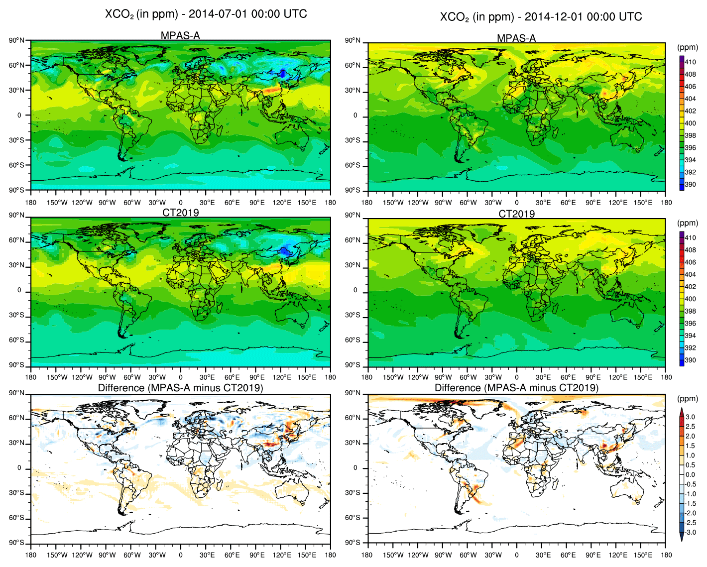
Figure 4 Simulated XCO₂ of MPAS-A, CT2019, and their difference on 1 July 2014 and 1 December 2014, 00:00 UTC.

First, XCO₂ values are calculated on the native grid for MPAS-A (60–15 km) and CT2019 (3^∘ × 2^∘). XCO₂ at a given model cell is calculated as the pressure-weighted CO₂ dry-air mixing ratio:

$$\begin{array}{}\text{(19)}& {\mathrm{XCO}}_{\mathrm{2}}=\left(\sum _{k=\mathrm{1}}^N{p}_k{q}_k^{{\mathrm{co}}_{\mathrm{2}}}\right)/\left(\sum _{k=\mathrm{1}}^N{p}_k\right),\end{array}$$

where p_k is modeled air pressure at layer k corrected for water vapor, $q_k^{{\mathrm{co}}_{\mathrm{2}}}$ is CO₂ dry-air mole fraction at the same level. N is the number of vertical levels in a model. Then, XCO₂ values from MPAS-A and CT2019 are regridded from their respective grids on an identical 1×1^∘ grid for a direct comparison. Figure 4 shows the comparison of XCO₂ from MPAS-A (top) and CT2019 (middle) and their difference (bottom) for 1 July and 1 December 2014 at 00:00 UTC. The figure shows that XCO₂ values from MPAS-A and CT2019 are generally consistent at large scales, but differences exist at small spatial scales. For instance, the difference in horizontal resolution between MPAS-A and CT2019 can be clearly observed in XCO₂ in July over both northeastern and southern China. In December, MPAS-A has a higher XCO₂ than CT2019 within the Arctic Circle and southern China. Overall, the differences between MPAS-A and CT2019 are evident. The magnitude of differences is mostly within 3 ppm, which is similar to the magnitude reported in Polavarapu et al. (2016) for the GEM-MACH-GHG model. Because both models used the same surface CO₂ fluxes, the difference in the simulated CO₂ fields is only caused by the different model transport: spatial resolution, dynamics, and physical parameterizations. The differences between MPAS-A and CT2019 are expected due to the differences in the two models' horizontal resolution, dynamics, and physical parameterizations. Because no CTM can be expected to have perfect transport, the acceptability of transport is generally judged through comparisons of model simulation with measurements.

3.3.3 Comparison with near-surface CO₂ measurements

This section compares MPAS-A simulated CO₂ with hourly measurements from 50 stations that were used for the IFS model evaluation in Agusti-Panareda et al. (2019). The information of the 50 stations, including location, elevation, intake height, reference, and type, is listed in Table 4. Like in Agusti-Panareda et al. (2019), only the highest intake level is used at towers that have multiple intake heights. When multiple observations within an hour are available (such as those with a 30 min or shorter time interval), they are averaged to yield a single hourly value. For a given station, this results in 744 (24×31) hourly measurements per month at the maximum.

The MPAS-A hourly CO₂ statistics, including RMSE, SE, and bias at the 50 stations, are listed in Tables S1 and S2 of the Supplement for January and July 2014, respectively. For comparison, Tables S1 and S2 also include the statistics from the IFS 9 and 80 km resolution simulations (Agusti-Panareda et al., 2019) at the same sites for the same time periods. Table S1 shows that RMSE of the MPAS-A simulated hourly CO₂ ranges from 0.17 ppm at the SPO station to 16.65 ppm at the KAS station. In comparison, the IFS simulations also resulted in a much lower RMSE at the SPO than KAS, the latter of which has a RMSE of 4.44 ppm from the 9 km resolution simulation and 10.71 ppm from the 80 km simulation.

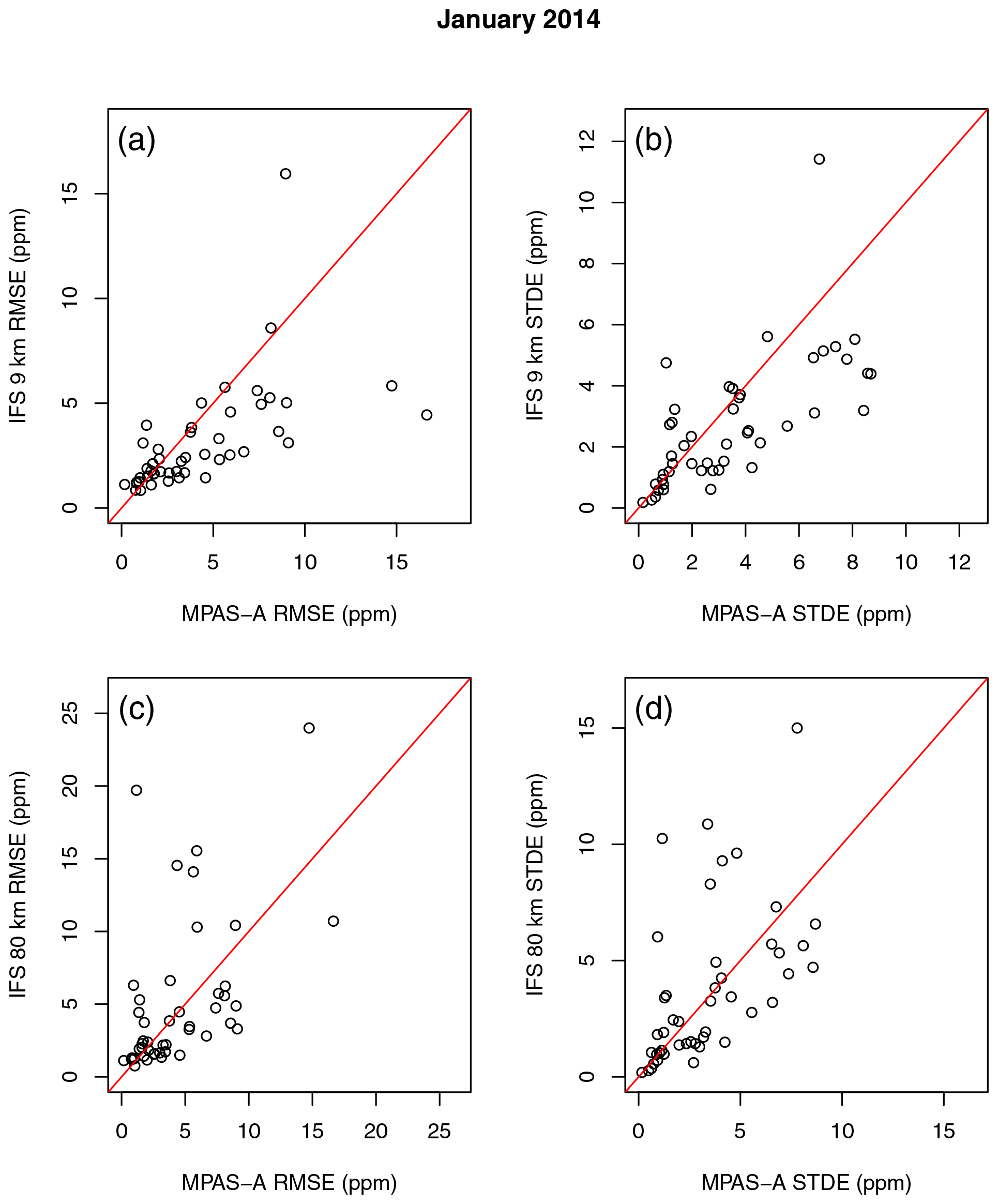
Figure 5 Comparison of model-simulated hourly CO₂ accuracy (RMSE and SE) between MPAS-A and IFS at 50 surface and tower stations. Each open circle in the figures represents a station. Comparisons of MPAS-A with the IFS 9 km resolution simulations are in panels (a) and (b), and comparisons with IFS 80 km resolutions simulations are in panels (c) and (d).

Figure 6 Same as Fig. 5 but for July 2014.

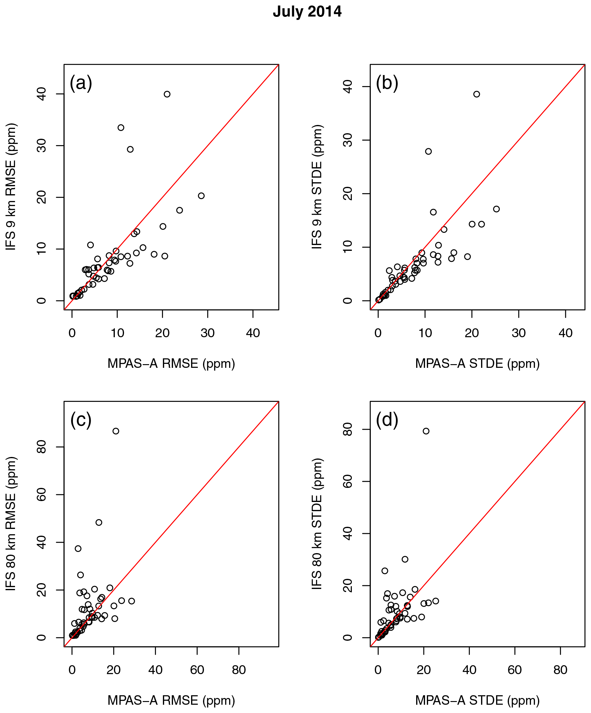
Table 5 Comparison of mean RMSE of hourly CO₂ from MPAS-A and IFS 9 km and 80 km simulations. p values of the paired t test between MPAS-A and the IFS simulations are also listed.

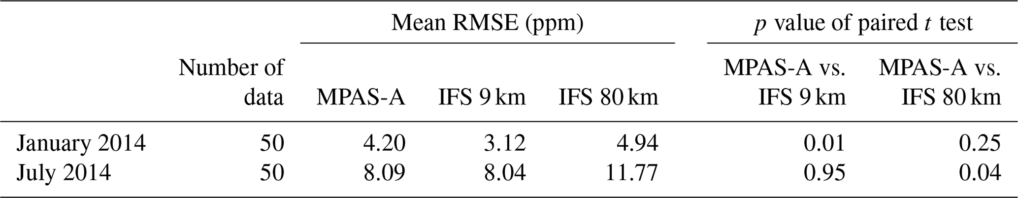
The comparisons of RMSE and SE from MPAS-A and IFS are shown in Figs. 5 and 6 for January and July 2014, respectively. Table 5 uses a paired t test to provide a quantitative summary of the hourly CO₂ RMSE between MPAS-A and the IFS 9 and 80 km simulations. The table shows that for January 2014, the mean RMSE at the 50 stations is 4.20 ppm from MPAS-A, which is higher than the IFS 9 km simulation (3.12 ppm, p=0.01) and similar to the IFS 80 km simulation (4.94 ppm, p=0.25). For July 2014, the mean RMSE at the 50 stations is 8.09 ppm from MPAS-A, which is similar to the IFS 9 km simulation (8.04, p=0.95) and lower than the IFS 80 km simulation (11.77 ppm, p=0.04). The above comparisons indicate that the 60–15 km MPAS-A simulation has a level of accuracy between the IFS 9 and 80 km simulations.

Table 6 Comparison of RMSE of hourly CO₂ between the MPAS-A 60–15 km simulation and the IFS 9 km and 80 km simulations at 12 mountain sites (Table 4). The left half of the table is for six mountain sites located in MPAS-A's 15 km cells and the second half is for six mountain sites located in MPAS-A's 60 km cells. The top half of the table is for January 2014 and the bottom half is for July 2014.

Feist et al. (2014)Deutscher et al. (2015)Notholt et al. (2014)Griffith et al. (2014a)Iraci et al. (2016)Sussmann and Rettinger (2015)Blumenstock et al. (2017)Kawakami et al. (2014)Hase et al. (2015)Sherlock et al. (2014)Wennberg et al. (2014b)Warneke et al. (2014)Wennberg et al. (2014a)De Mazière et al. (2014)Morino et al. (2016b)Kivi et al. (2014)Morino et al. (2016a)Griffith et al. (2014b)

Table 7 TCCON stations used for model evaluations.

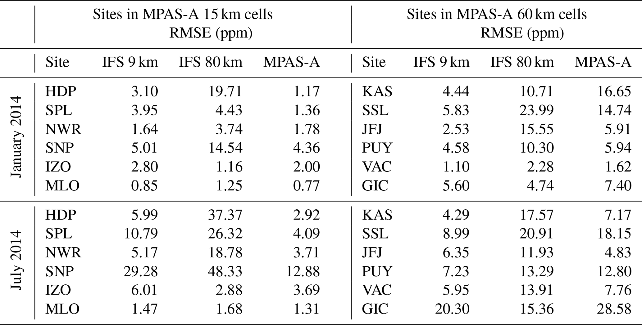
Agusti-Panareda et al. (2019) found that atmospheric CO₂ transport is generally better represented at higher horizontal resolutions, and mountain stations display the largest improvement at higher resolution as they directly benefit from the more realistic orography. There are 12 mountain stations of the 50 stations used for the model validation. Table 6 lists the 12 mountain stations in two groups: the first group includes the six mountain stations located in the 15 km cells of the MPAS-A's 60–15 km variable-resolution grid, and the second group includes the other six stations that are located in the 60 km cells of the grid. The table lists the hourly CO₂ RMSE for each of the 12 stations from MPAS-A and IFS 9 and 80 km simulations for January and July 2014. The table shows that at each of the six mountain stations located in 15 km cells, MPAS-A has lower hourly CO₂ RMSE than the IFS 9 km simulation for July 2014. For January 2014, MPAS-A has a lower RMSE than the IFS 9 km simulation at five out the six stations (the exception is NWR). In comparison, at the six mountain stations located in its 60 km cells, MPAS-A has higher hourly CO₂ RMSE than the IFS 9 km simulation for both January and July 2014 with the exception of JFJ for July 2014.

3.3.4 Comparison with TCCON XCO₂ measurements

After the comparison with the near-surface CO₂ in the last section, we evaluate MPAS-A CO₂ fields using XCO₂ measurements from 18 TCCON sites listed in Table 7. To compare with TCCON-retrieved XCO₂, smoothed MPAS-A XCO₂ is calculated following Wunch et al. (2010):

$$\begin{array}{}\text{(20)}& X_{{\mathrm{CO}}_{\mathrm{2}}}^{\mathrm{model}}=c_{\mathrm{a}}+{\mathbf{h}}^T{\mathbf{a}}^T({\mathbf{x}}_{\mathrm{m}}-{\mathbf{x}}_{\mathrm{a}}),\end{array}$$

where $X_{{\mathrm{CO}}_{\mathrm{2}}}^{\mathrm{model}}$ is the smoothed MPAS-A XCO₂, c_a is the a priori total column, a^T is TCCON column averaging kernel, h^T is a dry-pressure weighting function, x_m is MPAS-A CO₂ dry-air mole fraction profile, x_a is the a priori CO₂ dry-air mole fraction profile. The column profiles of CO₂, air pressure, and water vapor mixing ratio extracted from MPAS-A hourly output are interpolated to the same vertical grid as x_a, and the dry-pressure weighting function h^T is calculated following O'Dell et al. (2012) and Eq. (A7) of Agusti-Panareda et al. (2014).

Figure 7 Simulated hourly XCO₂ of MPAS-A at 18 TCCON sites for the year 2014.

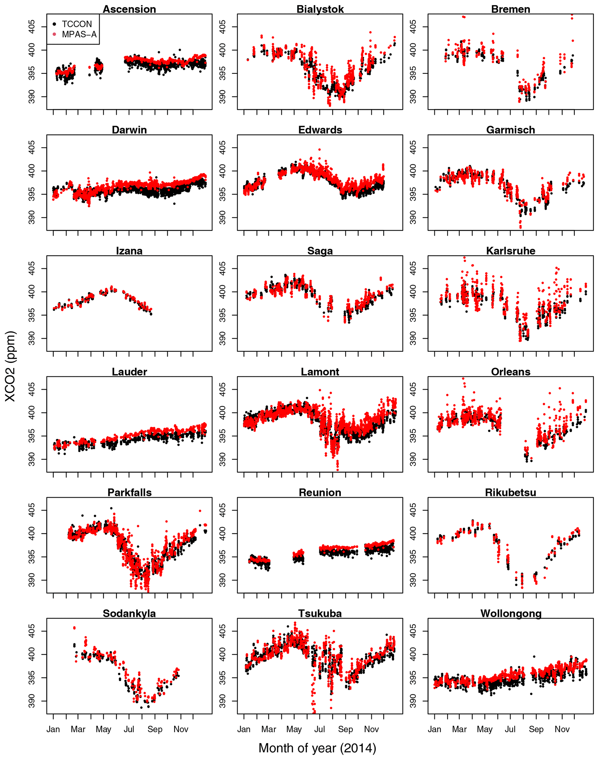
At a given TCCON site, averaged hourly XCO₂ (denoted as $X_{{\mathrm{CO}}_{\mathrm{2}}}^{\mathrm{TCCON}}$) is calculated as the mean value of all valid XCO₂ retrievals within the hour. $X_{{\mathrm{CO}}_{\mathrm{2}}}^{\mathrm{TCCON}}$ are then matched with the calculated hourly XCO₂ from MPAS-A (denoted as $X_{{\mathrm{CO}}_{\mathrm{2}}}^{\mathrm{model}}$). The comparisons of $X_{{\mathrm{CO}}_{\mathrm{2}}}^{\mathrm{model}}$ and $X_{{\mathrm{CO}}_{\mathrm{2}}}^{\mathrm{TCCON}}$ at the 18 TCCON sites for the year 2014 are shown in Fig. 7. The results indicate that the observed seasonal variations in TCCON XCO₂ are in general well represented by MPAS-A. The hourly average XCO₂ comparisons between MPAS-A and TCCON are summarized in Table 8. In the table, N is the number of data pairs used for calculating the statistics, including RMSE, bias, and correlation coefficient R. The mean RMSE of the 18 sites is 1.35 ppm, which is comparable to the IFS simulations (1.02 to 1.25 ppm) (Agusti-Panareda et al., 2019). We then calculated the average daily XCO₂ as the mean value of all the hourly XCO₂ within a given day. The statistics of the comparison of daily XCO₂ between MPAS-A and TCCON are also included in Table 8. In the table, N is the number of average daily XCO₂ used for calculating the statistics. Compared to their hourly counterparts, the average daily XCO₂ has both lower RMSEs and higher correlation coefficients. The mean value of the average daily XCO₂ RMSE of the 18 TCCON sites is 1.23 ppm, which is comparable to IFS simulations (0.97 to 1.25 ppm) reported in Agusti-Panareda et al. (2019).

Table 8 Statistics for the average hourly XCO₂ and average daily XCO₂ comparison between TCCON measurements and MPAS-A simulations: RMSE (ppm), bias (ppm), and correlation coefficient R. N is the number of data pairs used for computing the statistics.

3.4 Model evaluation at regional scale

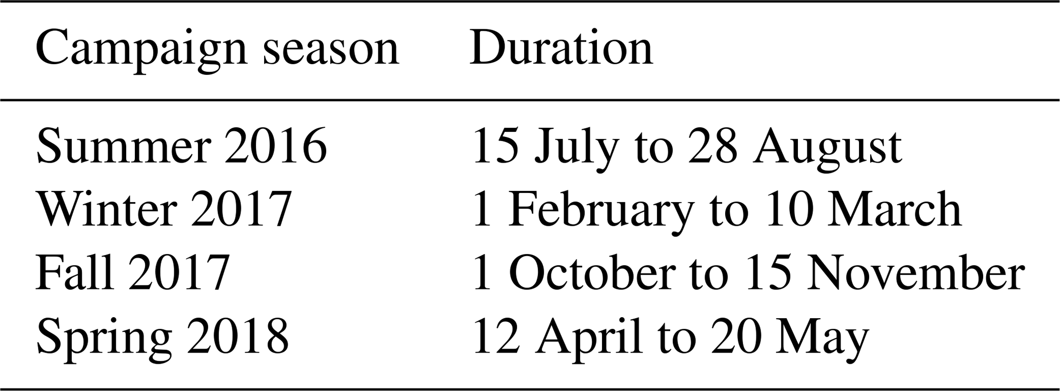
In this section, we present an evaluation of the MPAS-A CO₂ simulation accuracy using extensive high-resolution CO₂ observation data acquired through the ACT aircraft campaigns. ACT is a National Aeronautics and Space Administration (NASA) Earth Venture Suborbital 2 (EVS-2) mission, and its goal is to improve atmospheric inversion estimates of CO₂ and CH₄ through extensive airborne measurements over the eastern United States during multiple seasons (Davis et al., 2018a). Through four campaign seasons from summer 2016 to spring 2018 with two research aircraft (C130 and B200), the ACT project collected an extensive dataset of highly resolved CO₂ measurements in both the BL and FT. The duration of the ACT campaign seasons is given in Table 9. To use ACT airborne CO₂ measurements for model evaluation, we conducted a MPAS-A simulation from 1 January 2016 to 31 May 2018. The first 6 months are for the model spin-up. The simulation uses the domain and configurations as described in Sect. 3.1, and model outputs are saved at 1 h intervals.

Table 9 The duration of four ACT aircraft campaign seasons.

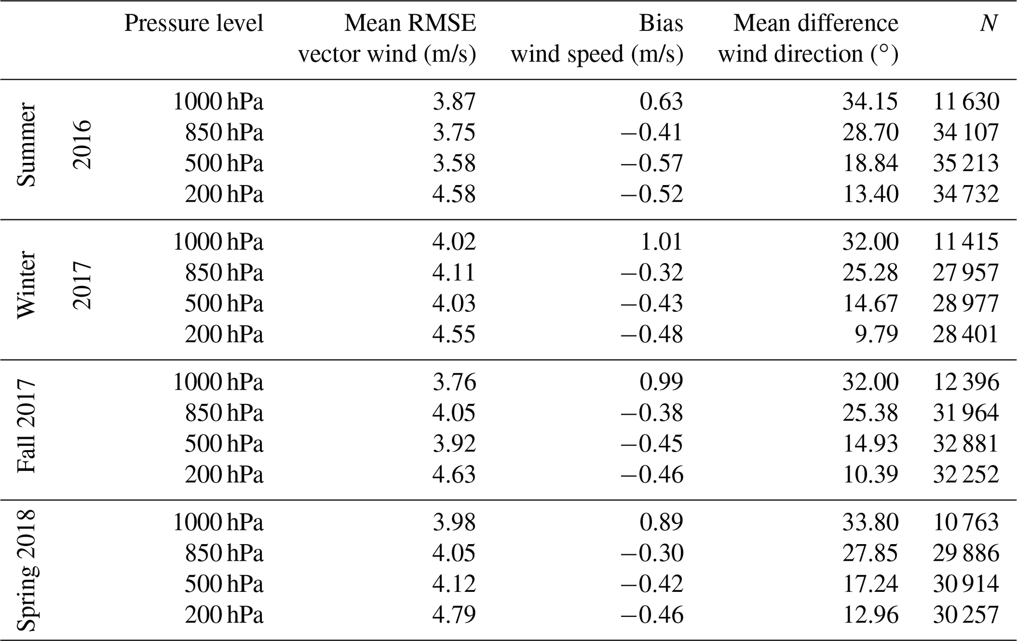
First, we compare MPAS-A simulated horizontal wind fields during the ACT campaign seasons using the same procedure described in Sect. 3.3.1. Table 10 lists the statistics of horizontal wind field evaluations during the four ACT campaign seasons. The table indicates the same pattern as in 2014 (Table 2): the mean RMSE vector wind increases with altitude and the mean difference of wind direction decreases with altitude. The magnitude of the statistics of the four ACT campaign seasons is comparable to that of 2014 (Table 2).

Table 10 Evaluation of the simulated horizontal wind of MPAS-A using radiosonde observations at 457 stations located across the globe. Wind speed and direction are compared at 00:00 and 12:00 UTC at four pressure levels (1000, 850, 500, and 200 hPa) for each day of the MPAS-A simulation. Note that the number of data samples (N) is smaller at 1000 hPa because some stations are located above that pressure level.

Next, we use the ACT campaign airborne measurements to evaluate the MPAS-A CO₂ simulation regarding its overall accuracy and its performance measured by three model evaluation metrics proposed by Pal et al. (2020). To provide an objective reference, we also compare MPAS-A performance with two established CO₂ model systems: WRF-Chem (Skamarock et al., 2008) and CT2019 (Jacobson et al., 2020) using the same set of airborne measurements. WRF-Chem is an online CTM based on the regional WRF model (Grell et al., 2011; Skamarock et al., 2008). WRF-Chem simulations have been carried out on a 27 km horizontal grid (Fig. S2) over North America as a part of the ACT campaign (Feng et al., 2020). The WRF-Chem simulations use ERA5 reanalysis (Hersbach et al., 2020) for meteorological initial and lateral boundary conditions, CarbonTracker (Jacobson et al., 2020) posterior mole fraction for CO₂ initial and boundary conditions, and CarbonTracker posterior fluxes for surface CO₂ fluxes. The WRF-Chem simulations use meteorological nudging and 120 h meteorological re-initialization to keep meteorological fields close to the reanalysis.

We use the ACT 5 s averaged CO₂ measurement dataset (Davis et al., 2018b), which has a horizontal resolution of approximately 500 m given the average aircraft velocity. MPAS-A simulated CO₂ fields are sampled as described in the second paragraph of Sect. 3 to match the 5 s airborne data points. WRF-Chem simulated CO₂ fields are also interpolated to match the ACT 5 s data point using the same approach as MPAS-A. CT2019 CO₂ used for the evaluation is obtained from CarbonTracker ObsPack (v5.0) (Masarie et al., 2014), which is the CT2019 posterior mole fraction interpolated to the ACT 5 s data points.

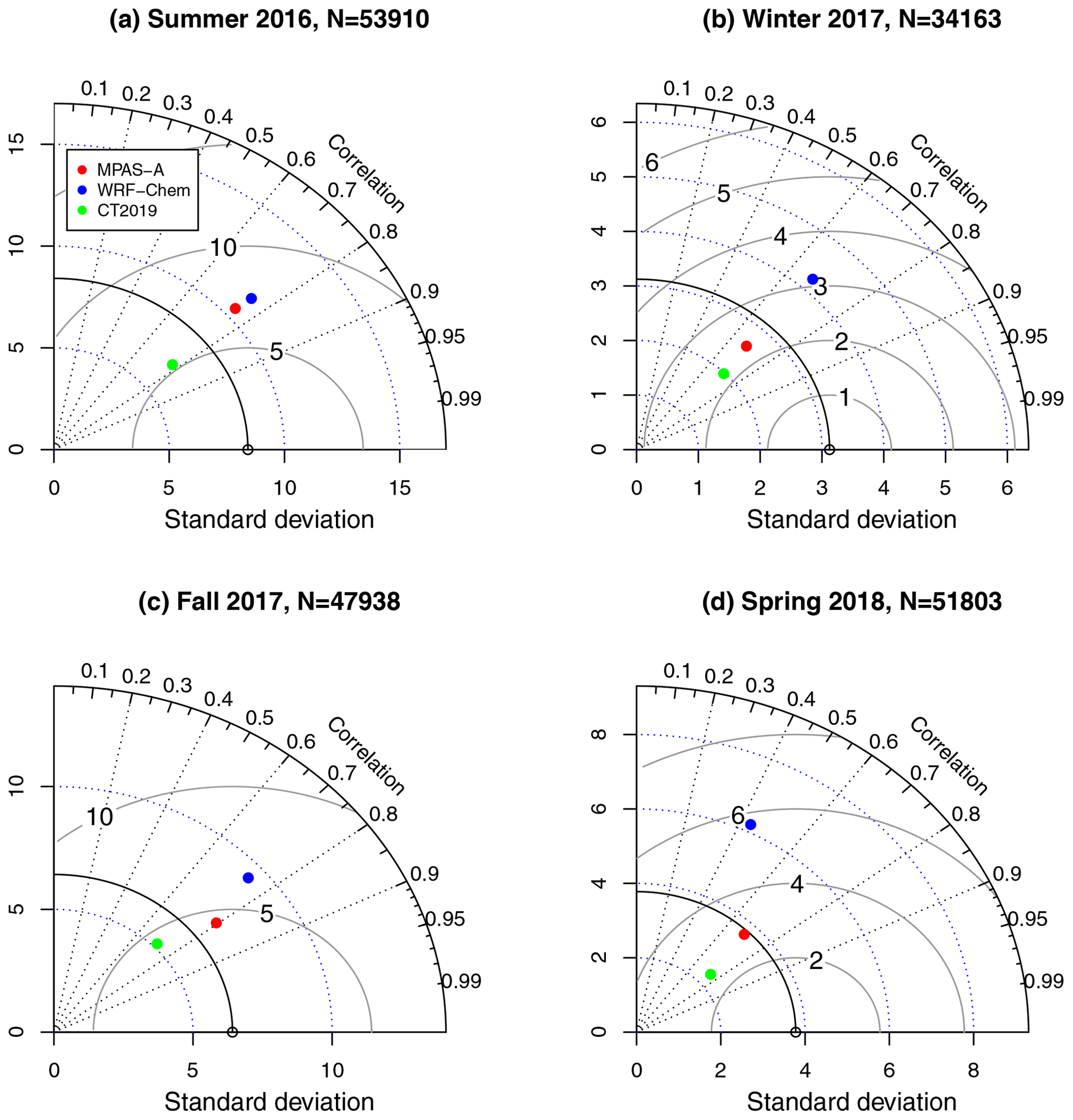
Figure 8 Taylor diagram for model evaluation using ACT airborne measurements in the boundary layer.

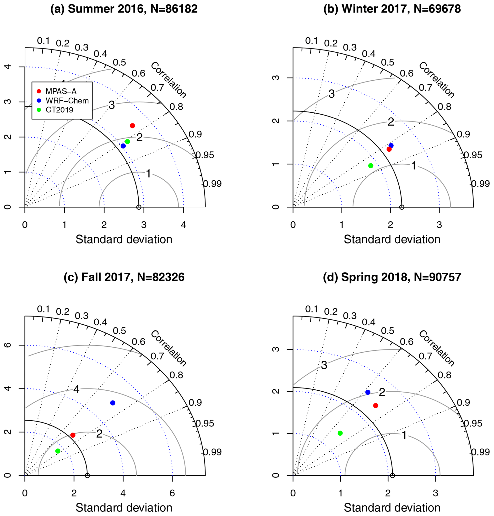
Figure 9 Taylor diagram for model evaluation using ACT airborne measurements in the free troposphere.

For each ACT flight day, CO₂ measurements from the two aircraft are combined if both are available, and their corresponding modeled CO₂ values from MPAS-A, WRF-Chem, and CT2019 are combined in the same way. With the four seasons combined, there are a total of 97 flight days (Pal and Davis, 2020), each one presented by an observation–model dataset consisting of observed CO₂, modeled CO₂ from the three models, along with the time, latitude, longitude, and altitude of each observation data point. Using the ACT maneuver flag dataset Pal et al. (2020), we further divide each flight day's data into two groups: one for BL and another for FT. For each ACT campaign season, all the BL data–model pairs are combined for each of the three models for model comparison. Figure 8 shows the Taylor diagram of the model comparison in the BL for the four campaign seasons. N in the title of each figure is the number of model–data pairs used for plotting the diagram. Similarly, the model comparison in FT is summarized in the Taylor diagrams of Fig. 9. A comparison of Figs. 8 and 9 shows that all three models have higher accuracy (lower RMSE) in FT than BL, which could be attributed to the larger error in the weather forecast in BL than FT associated with the accuracy of PBL height in the model simulation. Figure 8 shows that in BL, MPAS-A has a higher RMSE and higher standard deviation than CT2019. MPAS-A has more accurate estimation of the observations' standard deviation than CT2019 in all but summer 2016. Compared with WRF-Chem, MPAS-A has a lower RMSE and more accurate estimation of the observations' standard deviation. Figure 9 shows that in FT, MPAS-A has higher RMSE than CT2019 in all four campaign seasons and but it has more accurate estimation of the observations' standard deviation than CT2019 in all but the summer 2016 season. Compared to WRF-Chem, MPAS-A has lower RMSE and more accurate estimation of observations' standard deviation in all but summer 2016.

3.4.1 Model representation of CO₂ difference between warm and cold sectors

Through analyzing the ACT summer 2016 campaign data, Pal et al. (2020) identified three consistent features in the CO₂ mole fraction and proposed using these features as transport model assessment metrics. The three features are the differences between the warm and cold sectors, the difference between the BL and FT, and the CO₂ enhancement bands in the vicinity of frontal boundaries. Here and in the next two sections, we evaluate how MPAS-A simulated CO₂ represents the three features.

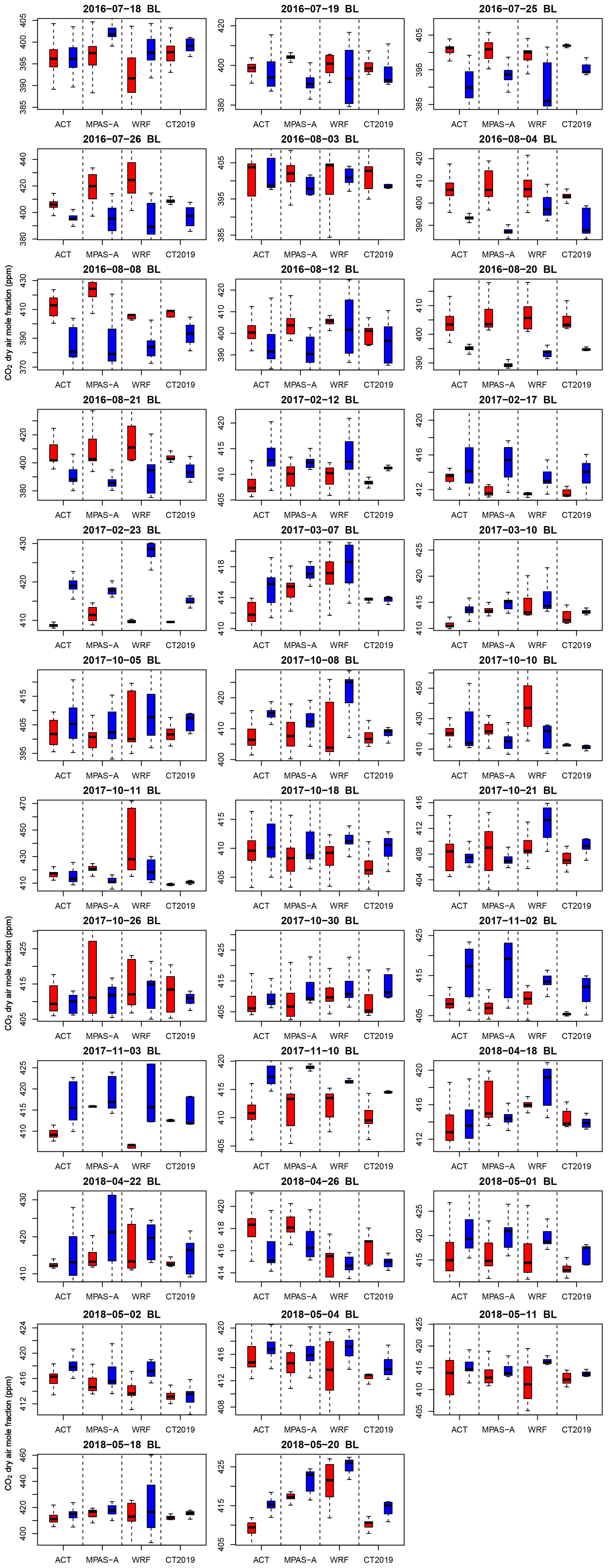
Figure 10 Box plots comparing mean boundary layer (BL) CO₂ mole fraction of the warm sector (red color) and cold sector (blue color) for 15 frontal crossing flights from summer 2016 and winter 2017 ACT campaign seasons. The flight date of each plot is labeled in its title. Data are combined when both aircraft (C130 and B200) took measurements for a given day. Each subfigure is separated into four groups by the dotted lines: the first group is from ACT observations, the second is from the MPAS-A simulation, the third is from the WRF-Chem simulation, and the last is from CT2019. In each box plot, the bottom and top edges of the box represent the first (Q1) and third (Q3) quartiles, the horizontal line represents the median, the ends of the whiskers represent Q1 − 1.5 × IQR (interquartile range) and Q3 + 1.5 × IQR, respectively, where IQR = Q3 − Q1.

Using the ACT maneuver flag dataset (Pal et al., 2020), we identified flights that crossed a weather front and their associated warm and cold sectors. The CO₂ mole fraction statistics for the warm and cold sectors are calculated from the aircraft measurements and the modeled CO₂ by MPAS-A, WRF-Chem, and CT2019, respectively. The results are shown in Fig. 10, which summarizes the statistics of CO₂ mole fraction differences between the warm and cold sectors measured by 15 front-crossing flights: 10 from the summer 2016 season and 5 from the winter 2017 season. The figure confirms that the warm sector has a higher average CO₂ mole fraction in the BL than the cold sector during summer 2016 as reported by Pal et al. (2020). The figure also shows that the average CO₂ mole fractions in the warm sectors are lower than those in the colder sectors in winter 2017, which is the opposite of what took place in summer 2016.

Table 11 Comparison of mean CO₂ dry-air mole fraction (ppm) in the boundary layer between the warm and the cold sectors. The table includes 10 frontal crossing flights from the summer 2016 season and 5 from the winter 2017 season. The column labeled “diff” is the mean value of the warm sector minus that of the cold sector.

Table 11 lists the mean CO₂ of the warm sector, cold sectors, and their difference as calculated from the ACT measurements, MPAS-A, WRF-Chem, and CT2019. The table shows that the MPAS-A simulations are similar to WRF-Chem, and both tend to have larger CO₂ differences between the warm and cold sectors than CT2019. For instance, the 8 August 2016 case where the observed mean CO₂ difference between the warm and cold sector is 26.9 ppm, MPAS-A and WRF simulations resulted in 36.9 and 21.2 ppm, respectively, while CT2019 resulted in a 15.3 ppm difference. The above evaluation indicates that the MPAS-A CO₂ model is capable of well representing the observed CO₂ difference between the warm and cold sectors, and its accuracy in this respect is comparable to WRF-Chem and CT2019.

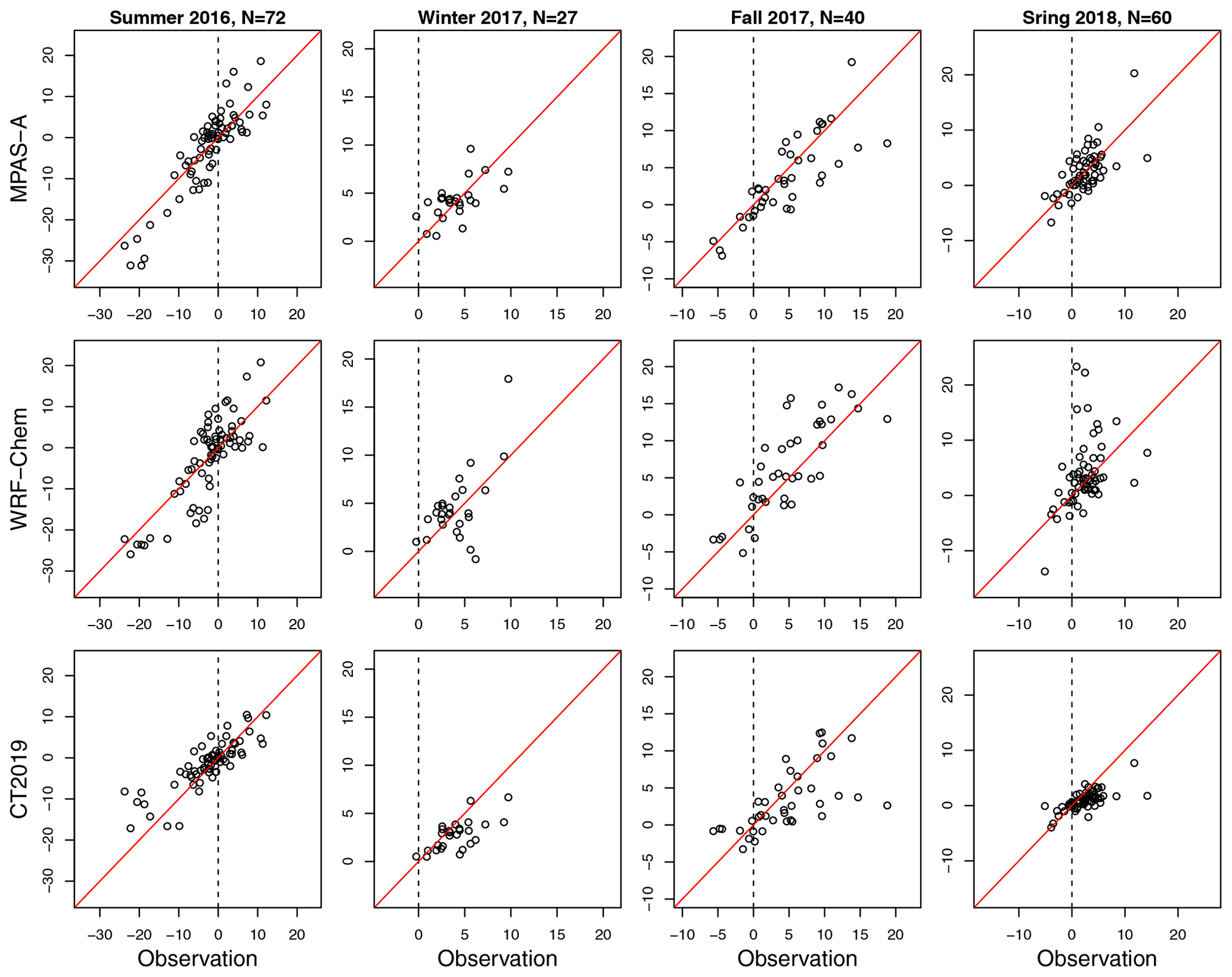
Figure 11 The difference of mean CO₂ mole fraction between boundary layer (BL) and free troposphere (FT) ($\mathrm{\Delta }\left[{\mathrm{CO}}_{\mathrm{2}}\right]=[{\mathrm{CO}}_{\mathrm{2}}{]}_{\mathrm{BL}}-[{\mathrm{CO}}_{\mathrm{2}}{]}_{\mathrm{FT}}$) at vertical profiling flight legs. In each subplot, each open circle represents an individual vertical profiling flight leg, and its values on the x axis and y axis represent its Δ[CO₂] value from the aircraft observations and the model simulation, respectively. Δ[CO₂] values from MPAS-A simulations are in the first row, WRF-Chem the second row, and CT2019 the third. The four columns in the figure are for the four ACT campaign seasons. The number of vertical profiles in each season is labeled in the column title. The vertical dashed line marks where Δ[CO₂]=0 based on the aircraft measurements.

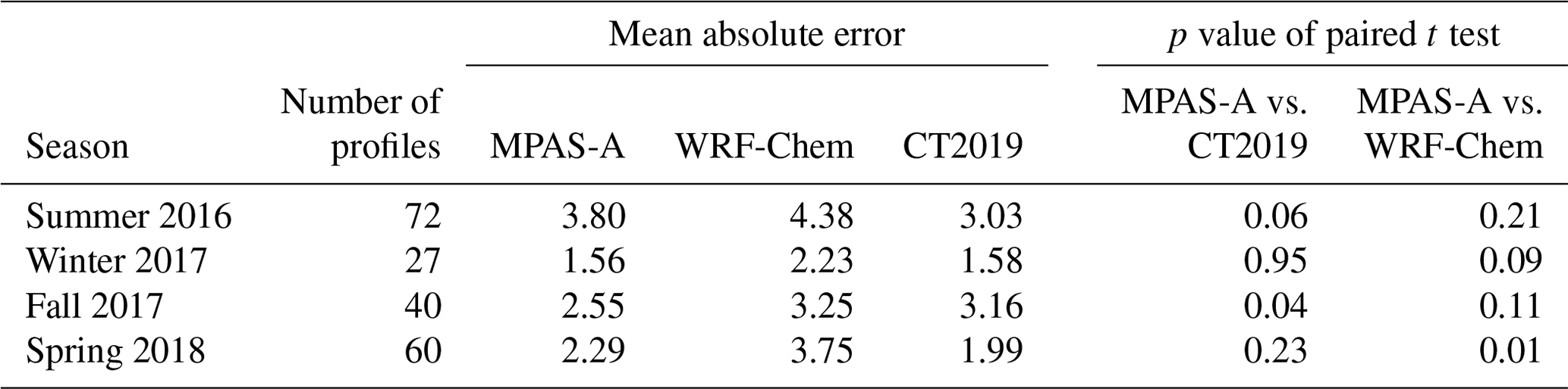
Table 12 Mean absolute error (MAE) of the simulated CO₂ of MPAS-A, WRF-Chem, and CT2019 as validated using ACT campaign aircraft CO₂ measurements. p values of paired t tests between MPAS-A and the other two models are included to provide a significance level for the model comparisons.

3.4.2 Model representation of CO₂ vertical difference

The second feature identified by Pal et al. (2020) is the vertical difference of CO₂ mole fraction between the BL and FT. During the ACT campaign season, two research aircraft (B200 and C130) took many vertical profile measurements during take-off, landing, spiral-up and -down, and inline ascent and descent maneuvers (Pal, 2019). These profile observations characterize the vertical variation of the atmospheric CO₂ mole fraction. From the vertical profile measurements taken during the summer 2016 season, Pal et al. (2020) calculated the mean CO₂ mole fraction in the BL and FT, denoted as [CO₂]_BL and [CO₂]_FT, respectively. They further defined BL-to-FT CO₂ difference as $\mathrm{\Delta }\left[{\mathrm{CO}}_{\mathrm{2}}\right]=[{\mathrm{CO}}_{\mathrm{2}}{]}_{\mathrm{BL}}-[{\mathrm{CO}}_{\mathrm{2}}{]}_{\mathrm{FT}}$. They found that Δ[CO₂] tends to be positive in the warm sector and negative in the cold sector. In this section, we evaluate how well MPAS-A represents the BL-to-FT CO₂ difference and compare its performance with WRF-Chem and CT2019.

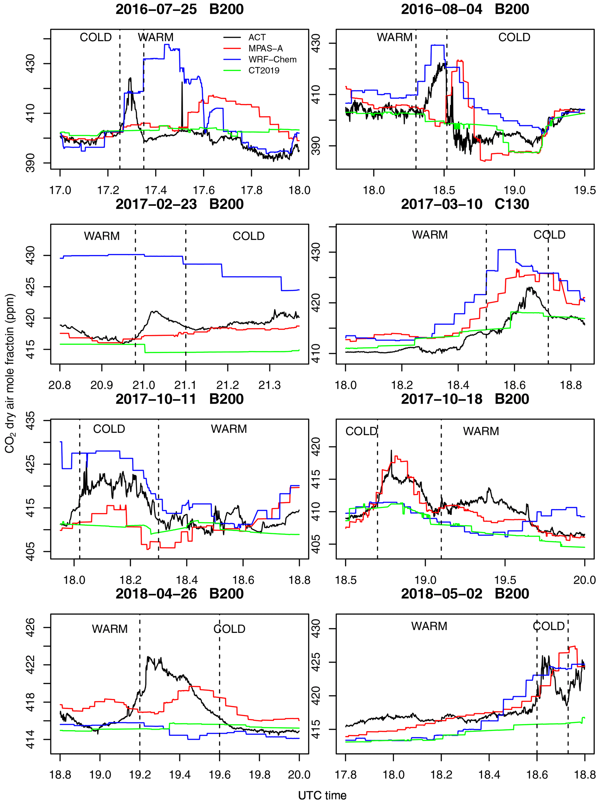
Figure 12 Comparison of CO₂ mole fraction in frontal-crossing constant altitude flight segments in BL between ACT aircraft measurements and model simulations. Flight date and aircraft type are labeled in title for each flight leg. The x axis indicates UTC time, and the y axis shows the CO₂ mole fraction (ppm). Aircraft measurements are in black, MPAS-A in red, WRF-Chem in blue, and CT2019 in green. In each figure, the pair of vertical dashed lines mark CO₂ enhancement observed by the aircraft along a frontal boundary, and the warm and cold sectors associated with the frontal boundary are labeled as warm and cold, respectively.

Using the ACT maneuver flag dataset (Pal et al., 2020), we identified all vertical profiles taken during the four campaign seasons, from which we selected profiles that meet two criteria: (1) a vertical profile must include at least 20 5 s measurements in the BL and 20 measurements in FT; and (2) a vertical profile must extend at least 2 km in the vertical direction. These two criteria are used to ensure that the resulting [CO₂]_BL and [CO₂]_FT are statistically representative. A total of 199 qualified vertical profiles are identified from the four campaign seasons, including 72 from the summer 2016 season, 27 from winter 2017, 40 from fall 2017, and 60 from spring 2018. For each of the vertical profiles, Δ[CO₂] is calculated for the aircraft CO₂ measurements, and the simulated CO₂ by MPAS-A, WRF-Chem, and CT2019. We compare Δ[CO₂] from the models with that from the observations to assess how each model represents the observed BL-to-FT CO₂ difference. Figure 11 shows the comparisons grouped by the campaign seasons. The figure indicates a clear distinction in Δ[CO₂] between the summer 2016 and the other three seasons: there is a substantial number of both positive and negative Δ[CO₂] in the summer 2016 season, but the vast majority of cases in the rest of the three campaign seasons have positive Δ[CO₂]. The positive BL-to-FT CO₂ differences from the winter 2017 season measurements could be at least partially attributable to the lack of CO₂ drawdown during the non-growing season. In comparison, the fall 2017 and spring 2018 seasons have more mixed results probably because of their partial overlap with the growing season. For the summer 2016 season, vertical profiles with negative Δ[CO₂] (lower mean CO₂ in BL than FT) suggest photosynthesis during the growing season, but those with positive Δ[CO₂] values are probably caused by the interaction between photosynthesis and frontal passage (Pal et al., 2020).

To compare the three models' accuracy in representing the BL-to-FT CO₂ difference, we calculated the mean absolute error (MAE) for each model during each season, where $\mathrm{AE}=\left|\mathrm{\Delta }\right[{\mathrm{CO}}_{\mathrm{2}}{]}_{\mathrm{model}}-\mathrm{\Delta }\left[{\mathrm{CO}}_{\mathrm{2}}{]}_{\mathrm{obs}}\right|$ (the absolute difference in Δ[CO₂] between a model and the ACT observations).

$$\begin{array}{}\text{(21)}& \mathrm{MAE}={\displaystyle \frac{\mathrm{1}}{N}}\sum _{i=\mathrm{1}}^N{\mathrm{AE}}_i\end{array}$$

Table 12 summarize the MAE of the three models for each season. The table shows that MPAS-A has smaller MAE than CT2019 in fall 2017 (p=0.04) and a larger MAE in summer 2016 (p=0.06). The differences between the two models in the other two seasons are not significant (p≥0.23). Compared with WRF-Chem, MPAS-A has smaller MAEs in winter 2017 (p=0.09) and spring 2018 (p=0.01), while differences in the other two seasons are not significant (p≥0.11). In summary, the above model evaluation and comparison demonstrate that MPAS-A CO₂ transport model is capable of representing the aircraft-observed CO₂ difference between the BL and FT at least as accurately as WRF-Chem and CT2019.

3.4.3 Model representation of CO₂ enhancement at frontal boundaries

The third feature identified by Pal et al. (2020) in the summer 2016 aircraft measurements is the bands of enhanced CO₂ close to frontal boundaries in BL. They found these CO₂ enhancement bands are typically about 100 km wide and speculated that it would require a 20 km horizontal resolution model to effectively represent the feature. In this section, we identify the frontal boundary CO₂ enhancements in the four campaign seasons and examine how well they are represented by MPAS-A.

Using the same approach as Pal et al. (2020), a total of 48 front-crossing constant-altitude flight segments are identified from the four seasons (15 from summer 2016, 5 from winter 2017, 17 from fall 2017, and 11 from fall 2018). To evaluate how well MPAS-A represents the frontal boundary CO₂ enhancements and compare its performance with WRF-Chem and CT2019, CO₂ mole fractions measured by the aircraft and simulated by the three models are plotted together for each of the identified front-crossing constant-altitude flight segments. Figure 12 includes eight of the front-crossing flight segments and the full set is included in Fig. S3 of the Supplement. For each flight segment in Fig. 12, the pair of vertical dashed lines mark CO₂ enhancement observed by the aircraft along a frontal boundary. The warm and cold sectors associated with the frontal boundary in each flight are labeled as warm and cold, respectively. The figure indicates that frontal boundary CO₂ enhancements can be identified in most but not all of the cases. For instance, there is no clearly identifiable CO₂ enhancement in the B200 flights on 23 April 2018 (Fig. S3).

Figure 12 shows that MPAS-A has a varying degree of success in simulating the frontal boundary CO₂ enhancements: it represents both the timing and the magnitude of the enhancements very well in some cases (4 August 2016 and 18 October 2017 by B200) but results in substantial errors in either the timing (25 July 2016, B200) or the magnitude (10 March 2017, C130) in other cases. The figure also shows that the MPAS-A simulated CO₂ is more similar to WRF-Chem than CT2019: CT2019 tends to substantially underestimate the magnitude of CO₂ enhancement, while MPAS-A and WRF-Chem tend to overestimate it.

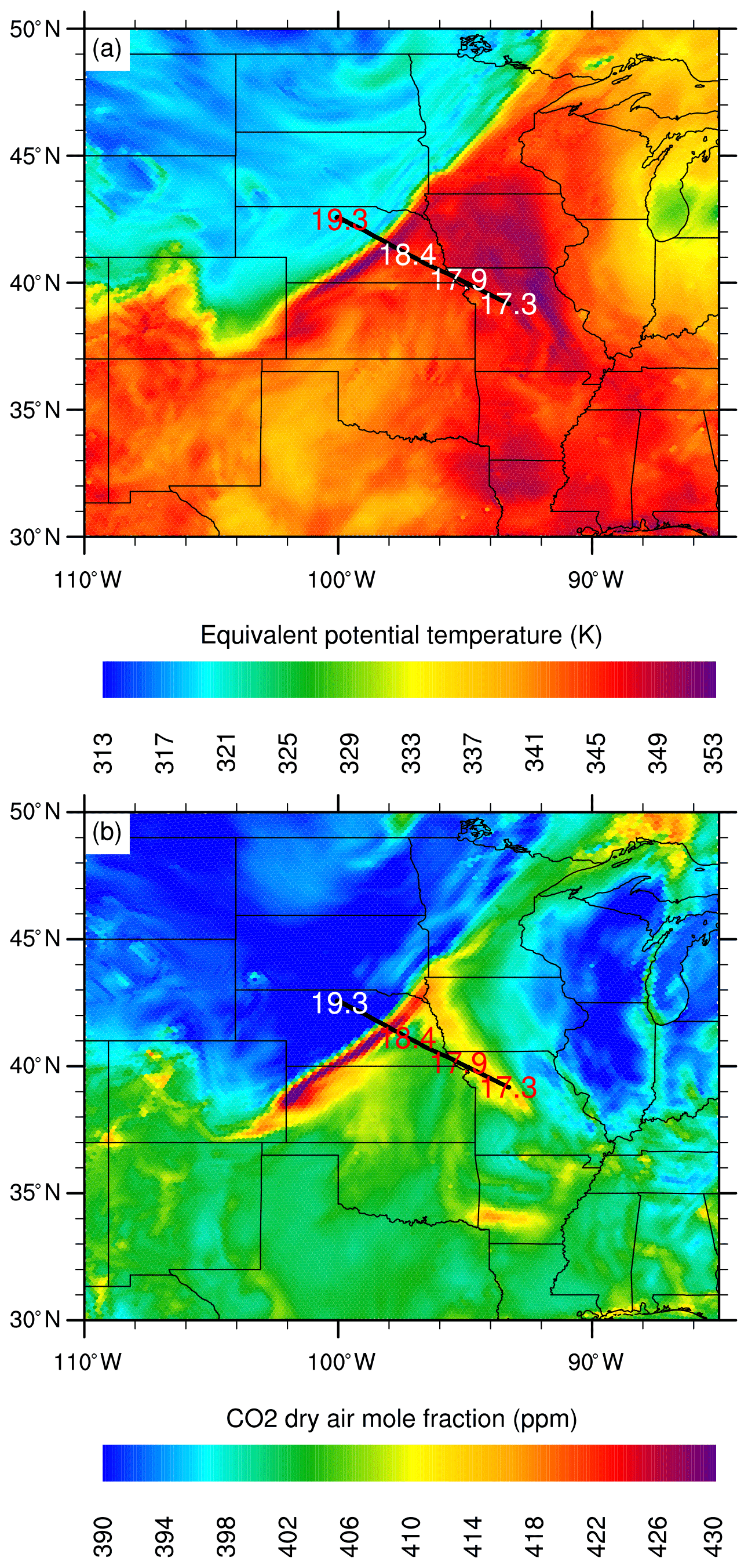
Figure 13 MPAS-A simulated equivalent potential temperature (θ_e, a) and CO₂ mole fraction (b) at 18:00 UTC on 4 August 2016. Both figures are plotted at the sixth MPAS-A vertical level, which is about 400 m above the ground.

Figure 13 shows the MPAS-A simulated equivalent potential temperature (θ_e) and CO₂ mole fraction at 18:00 UTC on 4 August 2016. The sharp boundary in θ_e indicates a surface cold front extending from southern Colorado northeastward to Wisconsin. Abrupt horizontal wind direction changes shown in Fig. S4 of the Supplement also indicate the cold front and its southeastward movement. Meteorological measurements taken during the flight (not shown) also confirm the cold front passage. The B200 research aircraft crossed the cold front from southeast to northwest at about 400–500 m above the ground between 17:15 and 19:15 UTC, and its flight track and timing are marked in Fig. 13. The aircraft measurements show an approximately 20 ppm enhancement along the front boundary, which can be clearly identified in the MPAS-A simulated CO₂ mole fraction (lower panel of Fig. 13).

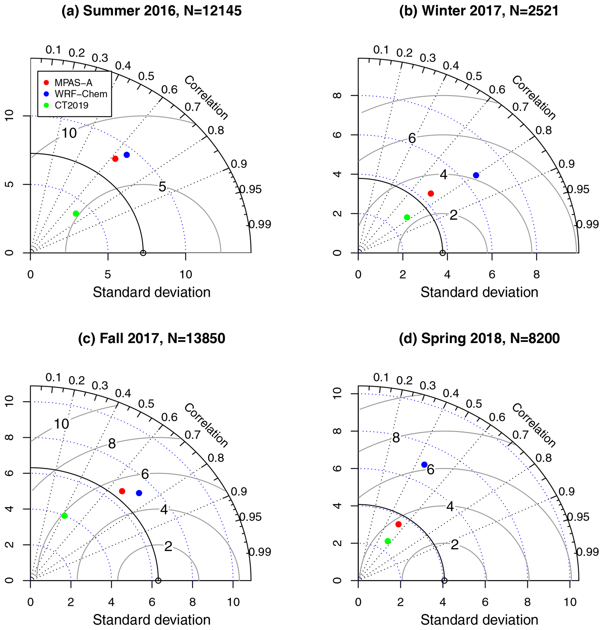
Figure 14 Taylor diagram for model evaluation using ACT airborne measurements from front-crossing flights. For each of the four ACT campaign seasons, observation–model data pairs from all front-crossing flights are combined. N is the number of data pairs used for creating the diagram.

Figure 14 compares the three models in their representation of the frontal boundary CO₂ variation. The figure shows that except for summer 2016, MPAS-A has a similar level of RMSE to CT2019, and it has a more accurate estimation of the observations' standard deviation. As horizontal resolution impacts a model's ability to represent small-scale spatial variability (Agusti-Panareda et al., 2019), the coarser resolution of CT2019 (1^∘ × 1^∘ over North America) is likely the primary cause of its underestimation of the frontal boundary CO₂ variability. MPAS-A has lower RMSE than WRF-Chem in winter 2017 and spring 2018, and it has a similar RMSE to WRF-Chem in the other two seasons. In all but summer 2016, MPAS-A has a more accurate estimation of the observations' standard deviation than WRF-Chem.

4 Summary

We implemented the CO₂ atmospheric transport processes, including advection, vertical mixing, and convective transport, in the global variable-resolution MPAS-A model. After the model development details were presented, simulation experiments designed for model evaluation were described. Two sets of simulations over a 60–15 km variable-resolution global domain were conducted for a model accuracy evaluation using an extensive aircraft measurements over the eastern United States and near-surface hourly measurements from surface and tower stations distributed across the globe. Meteorological initial conditions for these simulations are from the ERA-Interim analysis (Dee et al., 2011), and CO₂ initial conditions and fluxes are from CT2019 posterior mole fraction and flux products (Jacobson et al., 2020). To keep model meteorological fields close to the analysis, meteorology re-initialization is applied at 24 h intervals throughout the simulation periods. Global CO₂ mass conservation property is assessed by a 1-year continuous simulation without meteorology re-initialization and fluxes, and the results show that MPAS-A is capable of maintaining total dry-air mass conservation to the limit of machine precision. During the 1-year simulation period, the total CO₂ mass change is about 10⁻⁵ of its initial value. The larger variation of CO₂ mass than the dry air is due to the complex and strong spatial gradient caused by the surface CO₂ fluxes. Another 1-year simulation with meteorology re-initialization indicates that changes in dry-air density during the re-initialization causes changes in global total CO₂ mass, and a scaling method applied after each re-initialization is able to reduce the change from $\sim {\mathrm{10}}^{-\mathrm{4}}$ to $\sim {\mathrm{10}}^{-\mathrm{6}}$ of the global CO₂ mass.

The horizontal wind fields of the 60–15 km variable-resolution MPAS-A simulation are evaluated at four pressure levels at 457 radiosonde stations. Furthermore, a comparison with an additional 60 km uniform-resolution MPAS-A simulation shows that the accuracy of the horizontal wind fields is substantially higher at the 15 km cells. The accuracy of MPAS-A CO₂ transport is evaluated first at the global scale and then at the regional scale. At the global scale, MPAS-A simulation is evaluated using CT2019, near-surface hourly CO₂ measurements from 50 stations and XCO₂ measurements from 18 TCCON stations. The resulting statistics are compared with the ECMWF IFS 9 and 80 km resolution simulations over the same period conducted by Agusti-Panareda et al. (2019). The comparison indicates that RMSE of the MPAS-A simulation is similar to that of the 80 km IFS simulation but larger than that of the 9 km IFS simulation.

At the regional scale, a MPAS-A simulation extending from 1 January 2016 to 1 June 2018 is evaluated using the extensive high-resolution aircraft measurements from four ACT campaign seasons. Compared with a 27 km resolution WRF-Chem simulation and CT2019 posterior CO₂ mole fraction, MPAS-A simulated CO₂ achieves a comparable level of accuracy (as measured by RMSE). Further evaluation using three metrics proposed by Pal et al. (2020) shows that the MPAS-A simulation is capable of representing the observed CO₂ features as accurately as the WRF-Chem simulation and CT2019.

The model evaluations using the airborne and near-surface measurements indicate that the newly developed MPAS-A CO₂ transport model is capable of achieving a comparable level of accuracy with the more established CO₂ modeling systems, including the WRF-Chem regional model system, the CT2019 operational assimilation system, and the lower-resolution (80 km) simulation of the ECMWF IFS global CO₂ modeling system. Although further improvements are expected, the MPAS-A CO₂ transport model has the potential to contribute to improving our knowledge of atmospheric CO₂ transport and fluxes.