the Creative Commons Attribution 4.0 License.
the Creative Commons Attribution 4.0 License.
 | 26 May 2021
A Schwarz iterative method to evaluate ocean–atmosphere coupling schemes: implementation and diagnostics in IPSL-CM6-SW-VLR
Sébastien Nguyen
Pascale Braconnot
Sophie Valcke
Florian Lemarié
Eric Blayo
State-of-the-art Earth system models, like the ones used in the Coupled Model Intercomparison Project Phase 6 (CMIP6), suffer from temporal inconsistencies at the ocean–atmosphere interface. Indeed, the coupling algorithms generally implemented in those models do not allow for a correct phasing between the ocean and the atmosphere and hence between their diurnal cycles. A possibility to remove these temporal inconsistencies is to use an iterative coupling algorithm based on the Schwarz iterative method. Despite its large computational cost compared to standard coupling methods, which makes the algorithm implementation impractical for production runs, the Schwarz method is useful to evaluate some of the errors made in state-of-the-art ocean–atmosphere coupled models (e.g., in the representation of the processes related to diurnal cycle), as illustrated by the present study. IPSL-CM6-SW-VLR is a low-resolution version of the IPSL-CM6 coupled model with a simplified land surface model, implementing a Schwarz iterative coupling scheme. Comparisons between coupled solutions obtained with this new scheme and the standard IPSL coupling scheme (referred to as the parallel algorithm) show large differences after sunrise and before sunset, when the external forcing (insolation at the top of the atmosphere) has the fastest pace of change. At these times of the day, the difference between the two numerical solutions is often larger than 100 % of the solution, even with a small coupling period, thus suggesting that significant errors are potentially made with current coupling methods. Most of those differences can be strongly reduced by making only two iterations of the Schwarz method, which leads to a doubling of the computing cost. Besides the parallel algorithm used in IPSL-CM6, we also test a so-called sequential atmosphere-first algorithm, which is used in some coupled ocean–atmosphere models. We show that the sequential algorithm improves the numerical results compared to the parallel one at the expanse of a loss of parallelism. The present study focuses on the ocean–atmosphere interface with no sea ice. The problem with three components (ocean–sea ice–atmosphere) remains to be investigated.
- Article
(5135 KB) - Full-text XML
- BibTeX
- EndNote


For historical and physical reasons, present-day coupling algorithms implemented in coupled general circulation models (CGCMs) are primarily driven by the necessity to conserve energy and mass at the air–sea interface. However, the discretization of the coupling problem often leads to inconsistencies in time and space associated with the coupling algorithm and the grid-to-grid interpolation of air–sea fluxes and surface properties. In time, the coupling algorithms currently used in state of the art CGCMs do not provide the exact solution to the ocean–atmosphere problem, but an approximate one. Indeed, these approaches are mathematically inconsistent in the sense that they do not allow for a correct phasing between the ocean and the atmosphere. Roughly speaking, the existing coupling algorithms used in CGCMs split the total simulation time into smaller time intervals (called coupling periods) over which averaged-in-time boundary data are exchanged. The atmosphere computes the fluxes at the interface (heat, water and momentum), and the ocean computes the oceanic surface properties (water and sea ice temperatures, sea ice fraction, albedos, surface current). Two main algorithms are used: the parallel and the sequential atmosphere-first algorithm. In both methods, the interface fluxes for a coupling period are computed in the atmospheric model using the oceanic surface properties computed by the oceanic model and averaged over the previous coupling period. The two algorithms are lagged; i.e., there is a time lag (of one coupling period) between the model and its boundary conditions. They differ by the way atmospheric fluxes are used by the ocean. In the parallel algorithm, the ocean and atmosphere run concurrently, which adds a level of parallelism and reduces the time to solution. During a coupling period, the ocean run uses the interface fluxes of the previous one and computes the oceanic properties. Therefore, for a given coupling period, the fluxes used by the oceanic model are not coherent with the oceanic surface properties considered by the atmospheric model. In the sequential atmosphere-first algorithm, the atmosphere runs the coupling period while the ocean waits. This allows the ocean to use the fluxes of the present coupling period. The inconsistency is reduced, but not removed. The models cannot run concurrently, which suppresses a level of parallelism, except in the case of a two-coupling-period lag (see the RPN model described below). The parallel algorithm has been implemented in many European CGCMs used in CMIP6 besides IPSL-CM6, for example in CNRM-CM6-1 developed by CNRM-CERFACS (Centre National de Recherches Météorologiques – Centre Européen de Recherche et de Formation Avancée en Calcul Scientifique), EC-Earth3 developed by a Europe-wide consortium of 27 research institutes from 10 European countries, MPI-ESM (the Earth system model developed by the Max-Planck-Institut für Meteorologie) and HadGEM3-GC31 set up by the UK Met Office. The ocean–atmosphere coupling algorithm implemented in the CGCM developed at the European Centre for Medium-Range Weather Forecasts (ECMWF) is quite different and involves three components, an atmosphere model, a wave model and an ocean model run sequentially in that order, and it therefore corresponds to the sequential atmosphere-first algorithm. The CGCM developed by RPN (Centre de Recherche en Prévision Numérique) from the Canadian meteorological and climatic services (Environment and Climate Change Canada) also implements a sequential atmosphere-first algorithm, but with the particularity that the atmosphere receives and uses for one coupling period the surface properties calculated two coupling periods before by the ocean. This last algorithm allows us to run the models concurrently and therefore to keep this level of parallelism, but it increases the time lag and thus the inconsistency. To our knowledge, no model uses a sequential ocean-first algorithm.
Due to the overwhelming complexity of CGCMs, the consequences of inaccuracies in coupling algorithms for numerical solutions are hard to untangle unless a properly (tightly) coupled solution can be used as a reference. Schwarz algorithms are attractive iterative coupling methods to cure the aforementioned temporal inconsistencies and provide tightly coupled solutions. As discussed in Lemarié (2008), the standard coupling methods correspond to one single iteration of a global-in-time iterative Schwarz method. However, the theoretical analysis of the convergence properties of Schwarz methods is restricted to relatively simple linear model problems (e.g., Gander et al., 1999; Gander and Halpern, 2007; Lemarié et al., 2013). More recently, Thery et al. (2020) analyzed convergence for a coupled one-dimensional Ekman layer problem with vertical profiles of viscosities in both fluids. But there is no a priori guarantee that the iterative process converges in practice when implemented in tridimensional ocean–atmosphere coupled models.
Preliminary numerical simulations using the Schwarz coupling method for the simulation of a tropical cyclone with a realistic regional coupled model have already been carried out by Lemarié et al. (2014). Ensemble simulations were designed by perturbations of the initial conditions and of the length of the coupling period. One ensemble was integrated using the Schwarz method and another using a parallel algorithm, as described previously. The Schwarz iterative coupling method led to a significantly reduced spread in the ensemble results (in terms of cyclone trajectory and intensity), thus suggesting that a source of error is removed with respect to the parallel coupling case. For these experiments the iterative process converges when coupling fully realistic numerical codes (Lemarié et al., 2014), which strengthens our belief that Schwarz methods can be a useful tool in geophysical applications. Interestingly enough, a similar link between model uncertainties and consistency of the coupling method has been observed by Connors and Ganis (2011) in a coupled problem between two Navier–Stokes equations with interface conditions given by a bulk formulation.
The present study aims to assess the error made when using lagged coupling algorithms (parallel and sequential) in state-of-the-art CGCMs. To do so, a mathematically consistent Schwarz iterative method is implemented in the IPSL Earth system model. It is used as a reference to evaluate the error due to the lagged algorithms. We study the convergence speed, compare the methods and propose further developments in order to improve future ocean–atmosphere coupled models.
The paper is organized as follows. In Sect. 2, we detail the lagged coupling algorithms, taking as an example the IPSL model, and the Schwarz iterative method. Section 3 describes the model and the experimental set-up. Section 4 analyzes the results in terms of convergence speed and error assessment. Conclusions and future approaches are given in Sect. 5.
Multiphysics coupling methods used in the context of Earth system models can be classified into two general categories (e.g., Lemarié et al., 2015; Gross et al., 2018). The first one (usually referred to as asynchronous coupling and called lagged in the present paper1) is based on an exchange of average fluxes between the models. The second one (referred to as synchronous coupling in Lemarié et al., 2015) uses instantaneous fluxes. Climate modeling focuses primarily on how energy is exchanged between the Earth and outer space and is transported by the ocean and the atmosphere. When designing a coupling method in the context of CGCMs, water and energy conservation at machine precision are the key features. Those conservation principles are impossible to satisfy when exchanging instantaneous fluxes. Coupled ocean–atmosphere models used for long-term integration (decades to millennia) all use a coupling methodology based on the exchange of time-averaged or time-integrated fluxes.
2.1 Current ocean–atmosphere coupling in IPSL-CM6: the legacy parallel algorithm
Figure 1a describes how quantities are exchanged between the ocean and the atmosphere in the IPSL climate model from 1997 to now (Braconnot et al., 1997; Marti et al., 2010; Dufresne et al., 2013; Sepulchre et al., 2020; Boucher et al., 2020), knowing that both models are run in a parallel way. The coupling period Δt (which should not be confused with the dynamical time step in the individual models) typically varies between 1 h and 1 d, depending on the configuration and the model generation. Ocean and atmosphere dynamical time steps are always smaller but commensurable with the coupling period. To describe this coupling strategy, we introduce the atmospheric state vector 𝓐 (encompassing temperature, humidity, pressure, velocity, etc.) and the oceanic state vector 𝓞 (encompassing temperature, salinity, velocity, etc.). The time evolution of the atmosphere and the ocean is symbolically described by
where F𝓐 and F𝓞 are partial differential operators including parameterizations, and fΩ represents the fluxes at the ocean–atmosphere interface Ω. This formulation is symmetric between the ocean and the atmosphere. But, in practice, in CGCMs the symmetry is broken between the fast atmospheric component and the slower oceanic component. The fluxes are generally computed by the atmospheric component or by an interface model using oceanic surface quantities and atmospheric quantities taken in the vicinity of the air–sea interface (sea surface properties are denoted 𝓞Ω in the following), meaning that Eq. (1) can be reformulated as
With such an approach, the atmospheric model receives surface properties like sea surface and sea ice surface temperature, fraction of sea ice, albedo, and velocities of the surfaces (sea water and sea ice) and computes its own interfacial fluxes, which are then sent to the oceanic component. Interfacial fluxes sent by the atmosphere include heat fluxes (radiative and turbulent), water fluxes (solid and liquid precipitation, evaporation, sublimation) and momentum fluxes (wind stress).
As mentioned earlier, the coupling algorithm in the IPSL climate model is based on an exchange of averaged-in-time fluxes. We define as the time average in the interval [t1,t2] and Δt as the coupling period. A schematic view of the exchanges between the ocean and the atmosphere is given in Fig. 1. To run over a coupling period Δt, each component uses the available boundary conditions, which are time-averaged from the previous coupling period. We thus have the following.
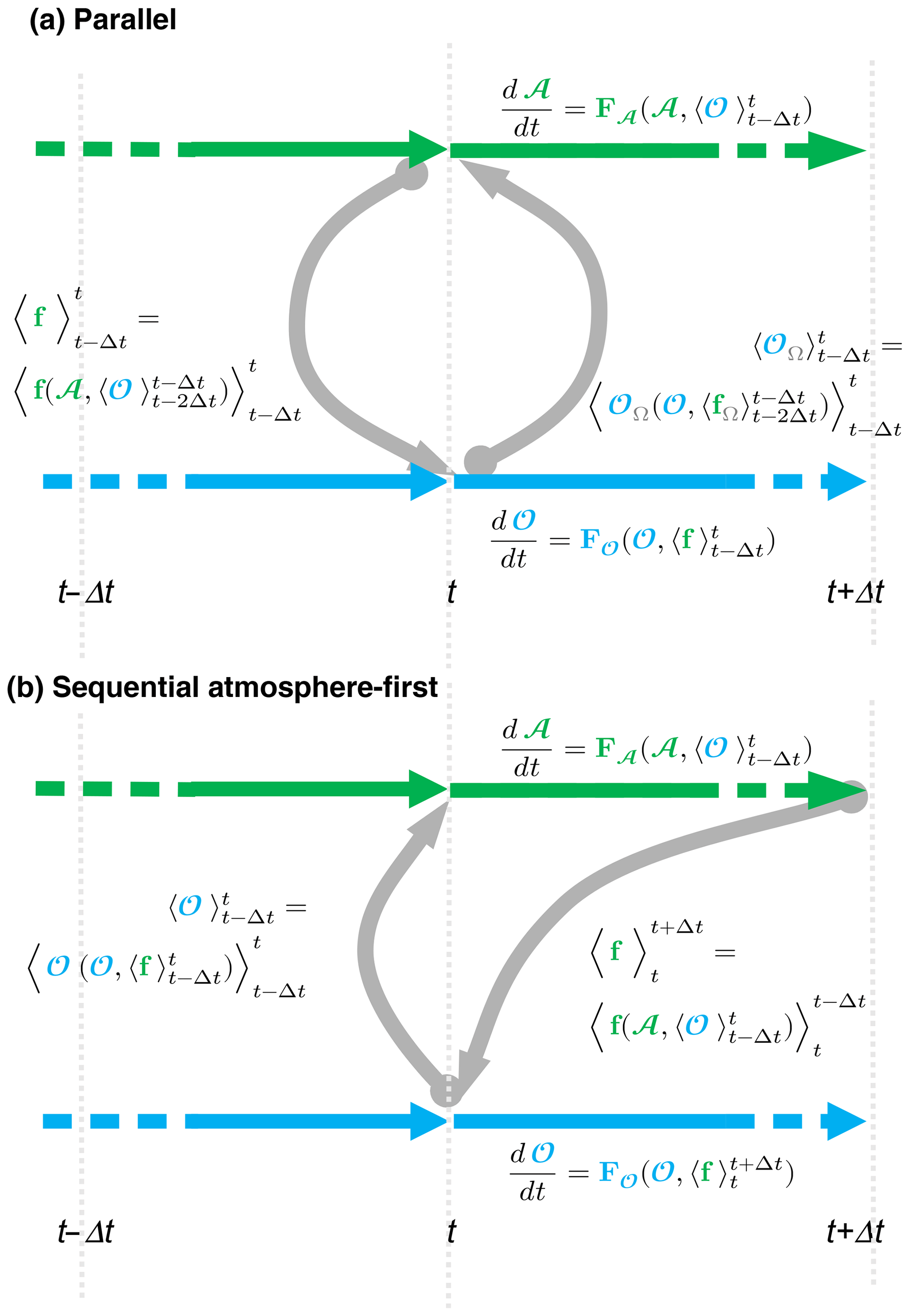
To be more precise, the fluxes sent from the atmosphere to the ocean and the surface properties sent from the ocean to the atmosphere at time t are as follows.
Substituting Eq. (4) in Eq. (3), we can thus write the evolution of the ocean 𝓞 and the atmosphere 𝓐 from t to t+Δt as follows.
The interfacial flux used as a boundary condition for the ocean between is computed by the atmosphere using sea surface values of the ocean from the time range . Symmetrically, the sea surface properties used to run the atmosphere during the time range are computed using surface values of the ocean from the time range . Equations (4) and (5) demonstrate the time shift between the two models and how the boundary conditions lag the models. The numerical solution thus obtained is not mathematically consistent and suffers from synchronicity issues, which may ultimately result in the numerical implementation being unstable in the sense that the error compared to the exact solution keeps increasing with time.
2.2 The sequential atmosphere-first algorithm
Figure 1b describes how quantities are exchanged between the ocean and the atmosphere in the atmosphere-first algorithm. The evolution of ocean 𝓞 and atmosphere 𝓐 become the following.
Substituting Eq. (7) in Eq. (6), we now have an asymmetry of the evolution of the ocean 𝓞 and the atmosphere 𝓐 from t to t+Δt.
This atmosphere-first algorithm has been easily implemented in IPSL-CM6 by changing lag parameters in the OASIS3-MCT coupler namelist. The symmetric ocean-first algorithm has been also implemented but is not detailed here.
To our knowledge, no coupled ocean–atmosphere model uses a coupling algorithm that is fully mathematically consistent. The survey of actual use cases (Valcke, personal communication) presented in the Introduction shows that they all induce a time lag between the models and the boundary conditions, either in both directions (double-sided lag) or at least in one direction (single-sided lag). In the GFDL Earth system model, the FMS coupler offers the possibility to use an implicit scheme to compute the interface quantities. But only the vertical turbulent diffusion part of the ocean and atmosphere models are considered (Balaji et al., 2006), and the full model equations are not synchronized.
2.3 The Schwarz iterative method
The Schwarz iterative method is described and analyzed in Lemarié et al. (2015) in the context of ocean–atmosphere coupling. The basic idea is to separate the global coupled problem in 𝓐∪𝓞 into separated sub-problems in 𝓐 and 𝓞, which can be solved separately with an appropriate exchange of boundary conditions at the common interface Ω. An iterative process is applied to achieve the convergence to the solution of the global problem. The main concern about this approach is the computational cost, which directly depends on the convergence speed.

Figure 2Stencil of the Schwarz iterative method, shown for the parallel algorithm; k is the iteration index. The ⋆ superscript denotes the converged solution. At each iteration k, the first guesses of 𝓐 and 𝓞 at time t are taken from the states of 𝓐 and 𝓞 at the end of the previous Schwarz window and for the last iteration. Only the boundary conditions are updated at each iteration.
As illustrated in Fig. 2, we iterate the system until convergence over the time interval . The first guesses of 𝓐 and 𝓞 at time t are taken from the states of 𝓐 and 𝓞 at the end of the previous coupling period . The iterative process from iteration k−1 to iteration k is described by the following.
In the classification of domain decomposition methods, such a Schwarz algorithm applied to the parallel coupling algorithm is called a parallel (or additive) Schwarz method, since it allows the concurrent resolution of the first two equations of Eq. (9). The Schwarz method applied to a sequential coupling simply consists of replacing the index k−1 by the index k in one of the first two equations. One then obtains a so-called sequential (or multiplicative) Schwarz method, which imposes the condition that the equation using the information at iteration k−1 be resolved first and then allows the resolution of the equation in the other medium. This sequential algorithm thus requires about twice the elapsed time of the concurrent version (if one considers that the elapsed times for each medium are balanced and that the two media run on different sets of processors or cores). However, it is well-known (and easy to prove) that in linear cases the sequential algorithm generally requires approximately 2 times fewer iterations to converge than the parallel algorithm.
For state-of-the-art CGCMs with complex parameterizations, we have no mathematical evidence that the algorithm converges. Indeed, as mentioned in Keyes et al. (2013), reaching a tight coupling between the components to be coupled requires smoothness. However, both ocean and atmosphere models include parameterizations that are potentially not differentiable. This is, for instance, the case of the bulk formulas used to compute the turbulent fluxes at the air–sea interface (e.g., Pelletier et al., 2018). A first step is thus to test the convergence when coupling realistic models. Assuming that the algorithm converges, for large values of k we would have , with the left superscript * denoting the converged solution. The evolution of *𝓞 and *𝓐 is given by
where it is clear that models and boundary conditions are now fully synchronized, meaning that the algorithm is mathematically consistent. In simple linear models, the unity of the converged solution is proven. It does not depend on the initial guess, which can be chosen arbitrarily. It also does not depend on the coupling algorithm: the parallel and sequential algorithms yield the same solution. However, different initial states will change the convergence speed. In our case, the models are strongly non-linear. The coupled problem may have several solutions, and the converged solution may depend on the initial guess. A relevant choice of the initial guess is then important. We use what is the most simple and obvious choice: the converged solution of the previous Schwarz window.
The Schwarz iterative procedure may span several coupling periods. The time interval is then called the “Schwarz window”. It is divided into p coupling periods. At the end of each Schwarz window, the models send the boundary conditions as a vector of values for the coupling intervals , . The boundary conditions exchanged between the models are then the vector of the following quantities.
With this method, the frequency of exchange can be different for each field, provided that the coupling period of each field is a whole division of the Schwarz window (the value of p is specific to each field). With more than two models, the Schwarz method can be used to couple models by pairs, for the whole system or for any relevant decomposition of the system. More details about the technical implementation in an Earth system model are given in Sect. 3.2. The following study handles only the case in which the Schwarz window is equal to the coupling period (p=1). The possibility to have a longer Schwarz window has not been coded for the sake of simplicity. Also, we did not test the algorithm with a lag of two coupling periods, as it would have been quite difficult to implement technically.
3.1 The IPSL-CM6-SW-VLR version of the IPSL Earth system model
At the start of this study, IPSL had two operational Earth system models available, IPSL-CM5A2-LR and IPSL-CM6-LR. IPSL-CM5A2-LR is an upgrade of IPSL-CM5A-LR (Marti et al., 2010; Dufresne et al., 2013) used by IPSL for the CMIP5 exercise, set up by Sepulchre et al. (2020). Compared to IPSL-CM5A-LR, the atmospheric model is tuned to reduce the surface cold bias and enhance the Atlantic meridional overturning circulation. The atmospheric code includes a supplemental level of shared memory parallelization that strongly improves the model scalability and speed. This model has an atmospheric resolution of in longitude–latitude and 39 vertical levels. It has an oceanic resolution of 2∘ and 31 vertical levels in the ocean. It runs at 70 simulated years per wall-clock day.
IPSL-CM6-LR (Boucher et al., 2020) is the model used by IPSL for the CMIP6 exercise. It has a higher resolution in both the ocean and atmosphere. All components (ocean, atmosphere, sea ice and land surface) have been improved with better physics compared to IPSL-CM5A2-LR. It runs at 10 simulated years per wall-clock day. The IPSL-CM6-LR computer code and running environment bring to the user a strong improvement in terms of performance, portability, readability, versatility and quality control. See Boucher et al. (2020) for details.
The present study uses the codes of IPSL-CM6 but runs at the resolution of IPSL-CM5A2-LR. As an iterative Schwarz method strongly increases the computing time, the choice of a low resolution allows us to contain the computing cost. As we planned high difficulties to implement the Schwarz method in the old-style coding of IPSL-CM5A2-LR, the choice of the newer code appeared obvious.
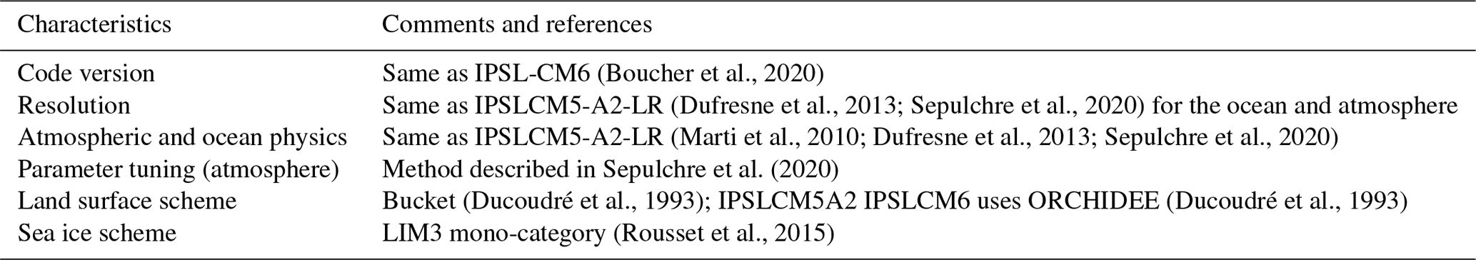
The parameters of the atmospheric model allow us to exactly reproduce the atmosphere of IPSL-CM5A2-LR when the atmosphere is run in stand-alone mode. In the ocean, the sea ice model LIM3 is used with one category of ice (IPSL-CM6-LR uses five ice categories based on ice thickness; see Rousset et al., 2015, for more details on LIM3 in the mono-category). The land surface model ORCHIDEE was removed to simplify and speed up the implementation of the Schwarz algorithm. As a soil model, we use the simple bucket model included in the atmosphere code (Ducoudré et al., 1993). The specificity of IPSL-CM6-SW-VLR with respect to IPSLCM5-A2-LR and IPSLCM6 is given in Table 1.
(Boucher et al., 2020)(Dufresne et al., 2013; Sepulchre et al., 2020)(Marti et al., 2010; Dufresne et al., 2013; Sepulchre et al., 2020)Sepulchre et al. (2020)(Ducoudré et al., 1993)(Ducoudré et al., 1993)(Rousset et al., 2015)Table 1IPSL-CM6-SW-VLR compared to IPSLCM5-A2-LR and IPSL-CM6.
This specific version of the model is called IPSL-CM6-SW-VLR for further reference, with SW standing for Schwarz. A short evaluation of the performance of IPSL-CM6-SW-VLR is given in Appendix A.
3.2 Implementation of the Schwarz algorithm in IPSL-CM6
The base of the Schwarz iterative algorithm is to repeat each Schwarz window with the same initial condition for each iteration, but with changing boundary conditions at the ocean–atmosphere interface Ω (the ones produced by the previous iteration). IPSL-CMs are restartable models: they produce the same result (bitwise) when run in one chunk or when the run is split into small chunks, with the final state of each chunk written to disk and read by the following one. In the ocean and atmosphere codes, we implement the possibility to save and/or restore the fields needed for a restart to and from the computer memory.
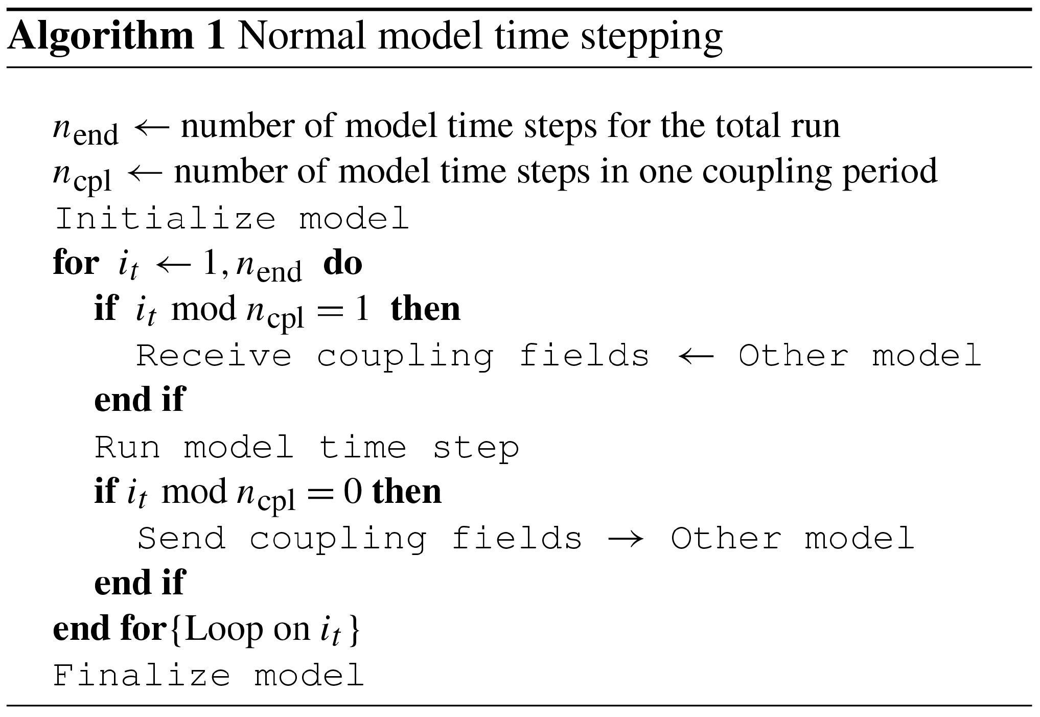
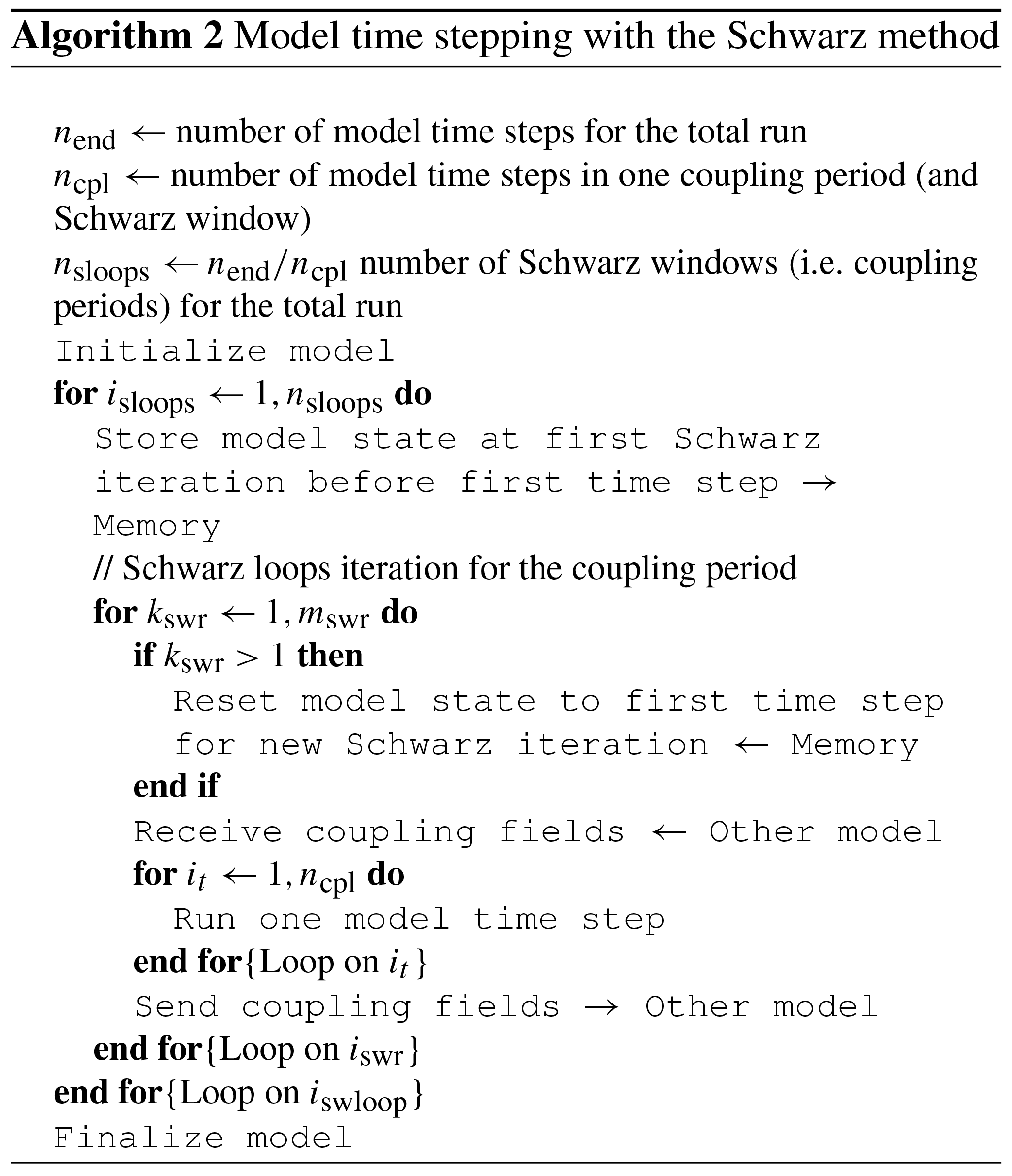
The time loop of the models is replaced by three nested loops. The outer one loops on coupling periods. The middle one loops over Schwarz iterations. The inner one loops over the model time steps inside a coupling period. (For a coupling period of Δt=1 h, the ocean performs two time steps and the atmosphere six time steps for the vertical physics, with 30 for the dynamics and one for the radiation scheme.) At the first Schwarz iteration of a Schwarz window, the initial state of the atmosphere 𝓐 and the ocean 𝓞 is the final state from the previous Schwarz window once the Schwarz iterations have converged. This state is saved in memory and will be read at the beginning of each iteration to initialize 𝓐 and 𝓞 with the same state for each Schwarz iteration. At the end of each iteration, the boundary conditions are sent to the companion model for use during the next one. The boundary conditions evolve during the iterative process. In this implementation, the length of the Schwarz window must equal the coupling period. The details of the different loops are given in Appendix B.
3.3 Experiments
We have run three sets of experiments (see Table 2). The first set uses the parallel algorithm. The second set uses the atmosphere-first algorithm. A third set uses the ocean-first algorithm. This last method is of no interest for operational use in a climate model, but it helped us to analyze some of the results. For each set, we run two experiments with coupling periods of Δt=1 h and Δt=4 h. The number of iterations is fixed to 50. The coupling fields exchanged between the models are written out at all iterations by the coupler OASIS, which allows us to study the convergence. Experiments are 5 d long (i.e., 120 and 30 Schwarz windows, or coupling periods in this case). The initial state is the end of a 50-year control experiment with pre-industrial forcings, run with the non-iterated parallel algorithm.
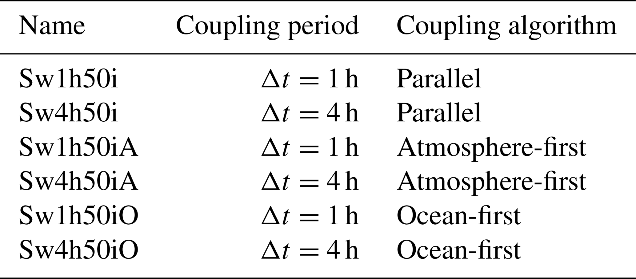

Figure 3Behavior of the sea surface temperature in four selected cases (i.e., instances of the Schwarz algorithm in space × time) for the parallel algorithm. For each graph, the yellow dots show the values at the end of the previous Schwarz window, when Schwarz has converged. This is the initial state of the present window. The green dots show the values after the first iteration. It is the value that the models use with the legacy parallel algorithm not iterated. The blue dots show the iterative process. Dots become grey when TΩ is considered to be converged. The two top cases (a, b) come from the Δt=4 h experiment. The bottom cases (c, d) come from the Δt=1 h experiment.
4.1 Convergence
Figure 3 shows the behavior of the sea surface temperature TΩ along the iterative process for four selected cases in time and space for the parallel algorithm. These cases represent typical behaviors. The yellow dots show the values at the end of the previous Schwarz window. This is the initial state of the Schwarz iterations for the present coupling period. The green dots show the values after the first iteration. It is the values that the models would compute without Schwarz. The blue dots show the iterative process. Dots become grey when TΩ is considered to be converged.
To decide if the convergence is reached at iteration kconv, we consider , the amplitude of the TΩ changes after the iteration kconv. . The convergence criterion is fulfilled if one of the following conditions is met:
-
oscillation from iteration kconv to 50 has an amplitude which is negligible compared to the total range of the signal, i.e., if ;
-
final oscillation from iteration k=kconv to k=50 has an amplitude AΩ(kconv) always lower than 10−4 ∘C for temperature and 10−2 W m−2 for heat fluxes;
-
oscillation has an amplitude from iteration kconv to 50 which is not bigger than the amplitude from iteration 41 to 50, i.e., . This last criterion supposes that convergence is always reached at iteration k=40. For points free of sea ice, this criterion is not necessary, as one of the two above is always verified.
The speed of convergence is sensitive to the definition of these criteria, which mostly come from a rule of the thumb rather than from a rigorous mathematical analysis. A small residual oscillation is observed in all cases. The mathematics of the Schwarz method for the ocean–atmosphere coupling have been developed in Lemarié (2008), Lemarié et al. (2014, 2015) and Thery et al. (2020). The theory is robust and well-established for two fluids with fixed turbulent viscosities. We have no theoretical frame when a third medium, sea ice in our case, is present. In all of the following, we will not analyze the behavior of the model when sea ice is present and study only ice-free points. Text and figures present the behavior of the sea surface temperature. When the sea surface temperature has converged, the atmosphere sees the same boundary condition at each iteration and computes the same fluxes. The converged solution computed in Eq. (10) is theoretically the same for the three algorithms (parallel and sequential). This means that the results should be the same for all experiments with the same time step. But convergence is not fully reached. A small oscillation remains. That means that at the end of the first Schwarz window, the solution is specific for each experiment. As small as it is, this difference explains why the experiments follow different trajectories, with the climate being chaotic.
Figure 4 shows a histogram of the number of iterations for all experiments. We consider all the instances of the iterative procedures for each ocean point of the atmosphere grid and for all Schwarz windows. As explained above, we consider only points with no sea ice. In the parallel Δt=1 h experiment, the Schwarz algorithm converges at the first iteration in almost 20 % of the cases. Two iterations are enough in almost 80 % of the cases. Only a few percent of cases require more iterations. The ocean-first algorithm slightly improves the result by a few percent. The atmosphere-first algorithm shows convergence at the first iteration for almost 100 % of the cases.
For the Δt=4 h experiments, convergence is rarely reached in one iteration. In most of the cases two to four iterations are required. We still observed that the parallel and the ocean-first algorithms yield close results, the second one being faster. The atmosphere-first algorithm strongly improves the speed of convergence.
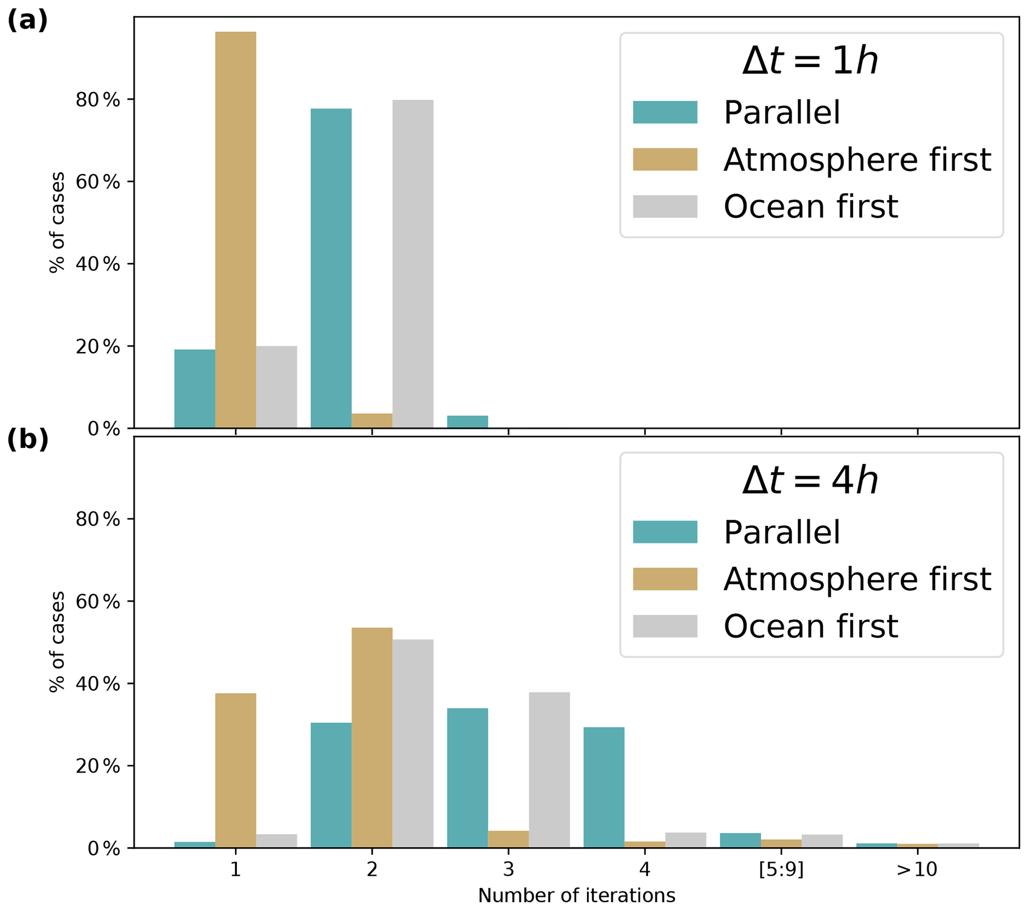
Figure 4Number of iterations for convergence for the (a, top) Δt=1 h and (b, bottom) Δt=4 h experiments. The total number of cases is 536 800=120 Schwarz windows ×4553 ice-free grid points in the Δt=1 h experiments and 136 800=30 Schwarz windows ×4560 ice-free grid points in the Δt=4 h experiments. This number of cases is given for the parallel algorithm and slightly differs for the other algorithms. The ordinates show the number of cases as a percentage of the total number of cases in time × space.
But the number of iterations might be sensitive to the choice of the convergence criterion. By construction, the convergence speed is in theory identical for all variables. After sea surface temperature (SST) convergence, the atmosphere uses the same values of SST at each iteration and computes the same fluxes. Symmetrically, when the fluxes computed by the atmosphere have converged, the ocean can do nothing but produce the same SST at each iteration. In practice, full convergence is not obtained, with a small oscillation of the values. As the convergence criterion is somewhat arbitrary, the computation of the number of iterations before convergence can give different values for the different variables. In the following, we diagnose the difference between the solutions with and without Schwarz, which does not depend on an arbitrary criterion.
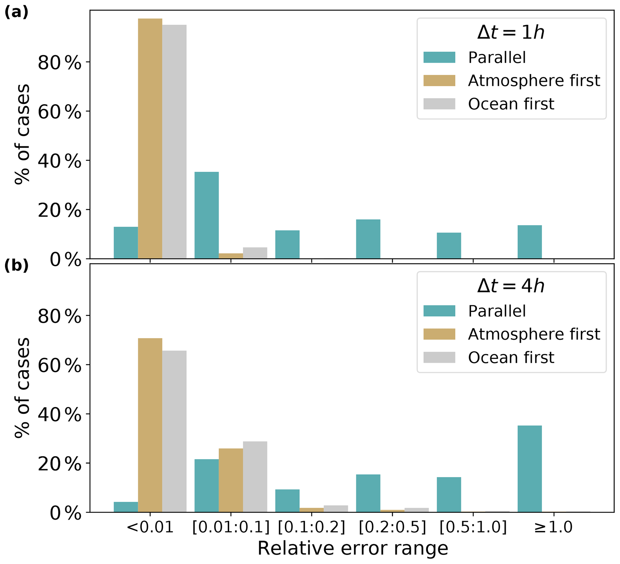
Figure 5Relative error of the change in sea surface temperature during a Schwarz window. The error is computed as the ratio between (i) the correction due to the iterative procedure (the jump from green dots to the converged solution in grey in Fig. 3) and (ii) the solution change between t and t+Δt with no Schwarz iteration (the jump from yellow to green dots in Fig. 3). See the legend in Fig. 4 for the explanation of the ordinate axis.
4.2 Diagnosing the error of lagged coupling
Figure 5 shows the relative error of the change in sea surface temperature during one coupling period when the Schwarz method is not used. The error is computed for the sea surface temperature (SST) trend during a coupling period. At each Schwarz iteration, the model computes an occurrence of the SST trend. At the first iteration, the trend is the one that the model would calculate with the legacy lagged coupling. We can then compare it with the trend obtained after convergence. This comparison of the two terms is done on a unique trajectory of the model. This trajectory uses the trend obtained at the last iterations. The error is computed as the ratio between (i) the correction due to the iterative procedure (the jump from green dots to the converged solution in grey in Fig. 3) and (ii) the solution change between t and t+Δt with no Schwarz iteration (the jump from green to yellow dots in Fig. 3).
In the parallel Δt=1 h experiment, the relative error is negligible (less than 0.01) in about 15 % of the cases. It is small (less than 0.1) in almost 50 % of the cases. But it is larger than 0.1 for the other half. The relative error is even larger than 0.5 in 25 % of the cases. The atmosphere-first experiment shows strongly improved results, with a negligible error for 97 % of the points. The conclusion for experiment ocean-first is somewhat different from what the histogram of iterations (Fig. 4) shows. The results are very close to the atmosphere-first experiments. For the Δt=4 h experiments, the errors are larger than in the Δt=1 h case, but with the same hierarchy between the algorithms. In Appendix C, we show that these conclusions are robust when analyzing the error in other interface variables.
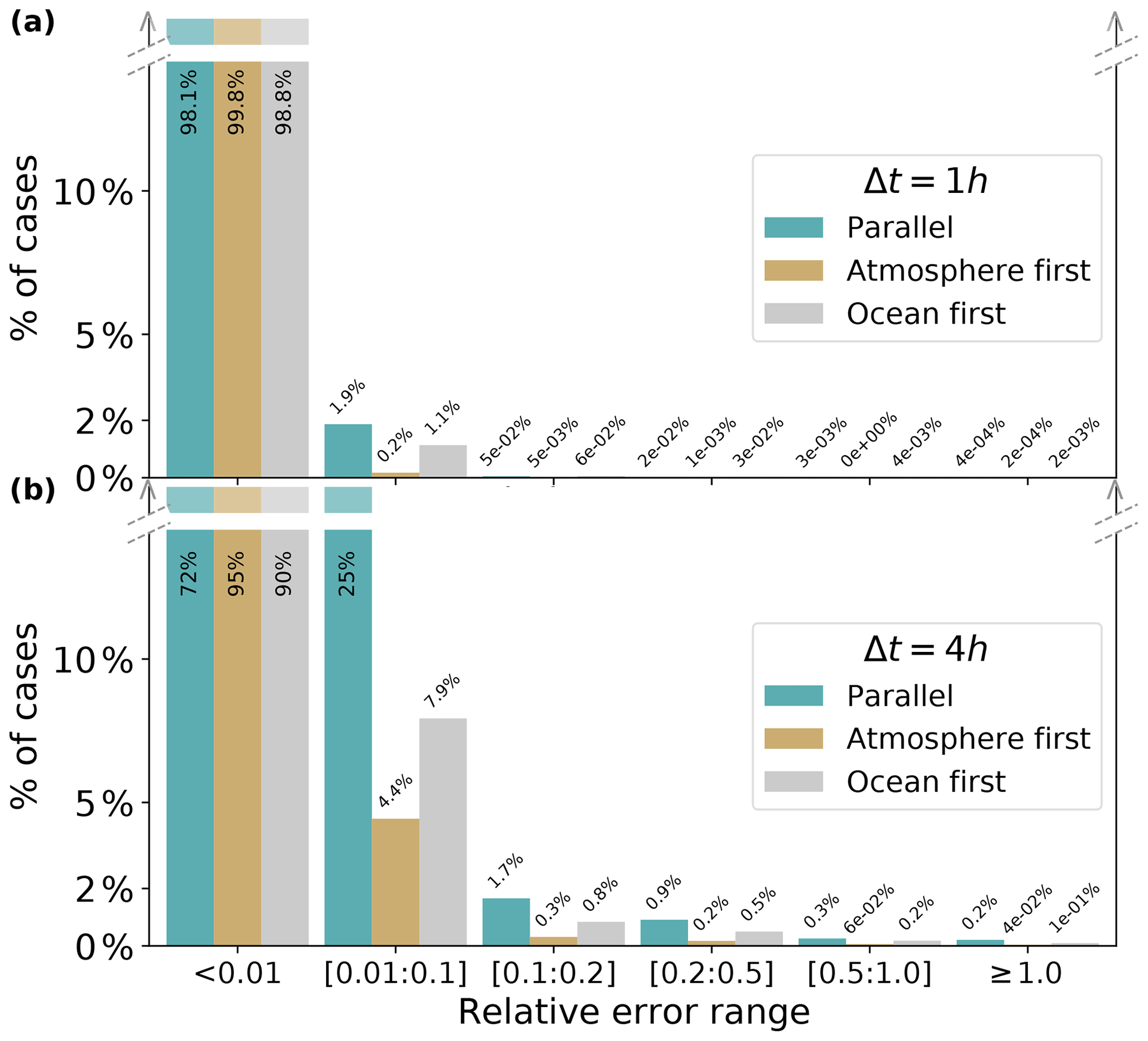
Figure 6 shows the relative error that would remain if we had stopped the Schwarz method at two iterations. The histogram shows that for the parallel Δt=1 h experiment, which is the slowest-converging one, non-negligible errors (> 0.01) account for only about 2 % of the cases. For small coupling periods, a two-iteration Schwarz method strongly improves the solution for the parallel algorithm, with only a handful of cases that need more than five iterations to reach a small error (less than 0.1, not shown). All these points are at the ice edge, where the convergence is slower. For the parallel Δt=4 h experiment, 25 % of the cases have an error in the range [0.01,0.1]. The number of cases with error larger than 0.1 after two iterations amounts to about 3.5 %. This is still a large improvement compared to the non-iterated parallel algorithm.
These results are coherent with the theoretical results on Schwarz methods mentioned previously. The sequential Schwarz method requires approximately 2 times fewer iterations to converge than the parallel algorithm. In IPSL-CM6-SW-VLR, both sequential algorithms converge faster than the parallel algorithm.
This result is not symmetric: the sequential atmosphere-first algorithm converges faster than the sequential ocean-first algorithm. We propose two hypotheses to explain this phenomenon. First, the characteristic timescales are longer in the ocean than in the atmosphere, and the diurnal cycle is more marked in the atmosphere than in the ocean. Therefore, using the information from the ocean in the previous time window to force the atmospheric model in the next time window is probably generally less problematic than doing the opposite. The atmospheric solution after the first half-iteration will then already be quite close to its converged value and will provide a relevant and synchronized forcing to compute the oceanic solution in the second half-iteration. Second, the better performance of the atmosphere-first case can also be linked to the phasing of the solar radiation, which is the only external forcing and constrains the diurnal cycle. In the parallel and ocean-first cases, the ocean is forced by fluxes, including solar radiation, calculated at the previous coupling period. In the case of atmosphere-first, the solar forcing is correctly phased.
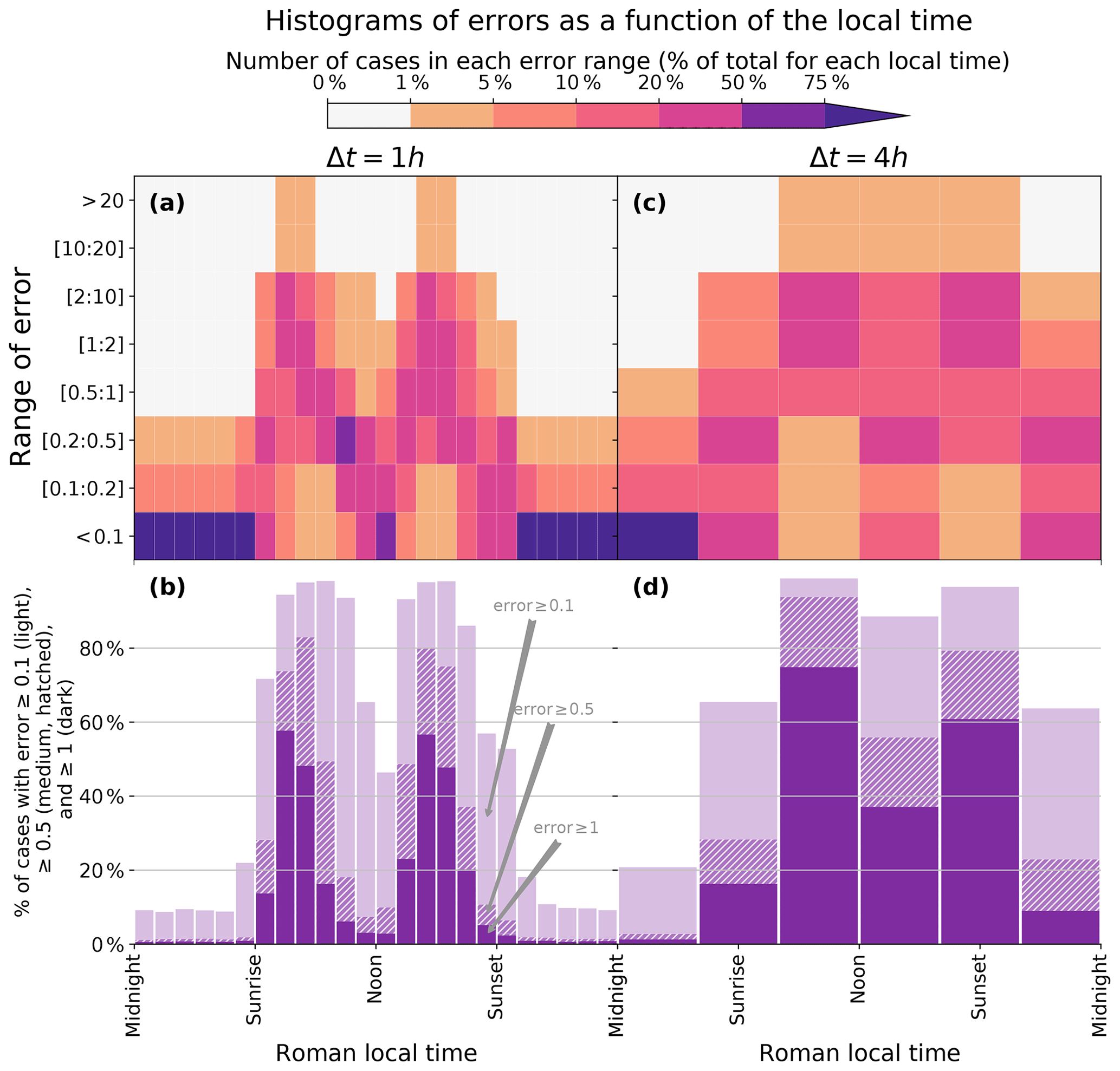
Figure 7Histograms of errors as a function of the Roman local time and error classes for the parallel experiments. Left panels (a, b) are for Δt=1 h and right panels (c, d) for Δt=4 h. Top (a, c) panels show the percentage of cases in space × time in each range of error as a function of the Roman local time. The Roman local time is the local time piecewise-stretched: the time from midnight to sunrise is divided into 6 regular pseudo-hours. The same method is applied to the intervals sunset to noon, noon to sunset and sunset to midnight. This is similar to the division of the day in ancient Rome (Wikipedia, 2020). The percentages are computed with respect to the total number of cases for each local time. Bottom panels (b, d) show the number of cases with errors larger than 0.1 (light purple), 0.5 (medium purple with hatches) and 1.0 (dark purple).
4.3 The diurnal cycle of the error
Figure 7 plots the SST trend error as a function of the Roman local time and error classes for the parallel experiments (see figure caption for the definition of Roman local time). The error histograms show a well-defined diurnal cycle with the lowest errors during the night. In both experiments, but mostly for Δt=4 h, errors are larger at noon than at midnight. The error is maximum after sunset and before sunrise, when the change in the insolation forcing evolves at the fastest pace. This pattern is clear for Δt=1 h. With Δt=4 h, the diurnal cycle of insolation is badly resolved, but the diurnal cycle of the error is still present. After sunrise and before sunset, 45 % of cases in time × space show an error larger than 1 for the Δt=1 h case. At these times of the day more than 70 % of the cases show error larger than 0.5, and almost all cases have non-negligible errors (≥ 0.01). All figures are slightly bigger for the Δt=4 h case.
An error larger than 1.0 means that the correction due do the Schwarz method is larger than the solution jump due to the lagged algorithm. In both experiments, the error of the parallel algorithm after sunrise and before sunset can affect the most important part of the solution computed by an Earth system model.
Present time algorithms used to couple the ocean and atmosphere in state-of-the-art Earth system models are mathematically inconsistent in all implementations we are aware of. The components are not correctly synchronized with their boundary conditions (Lemarié, 2008; Lemarié et al., 2014). A mathematically consistent Schwarz iterative method has been implemented in the IPSL coupled model to solve the ocean–atmosphere interface. This implementation yields a multiplication of the computing cost by the number of iterations. Although such a method is thus not affordable for climate studies, the Schwarz iterative method is used as a reference to evaluate the error made with the parallel and the sequential atmosphere-first algorithms currently used by many ocean–atmosphere modelers. The sequential ocean-first algorithm has also been tested.
We use the solution obtained with the Schwarz iterative method as a reference to diagnose the error in six experiments with the three coupling algorithms and two coupling period lengths of Δt=1 h and Δt=4 h. In the parallel algorithm, the error is quite large, with the highest values after dawn and before dusk when the change in insolation at the top of the atmosphere, the only external forcing, has the highest rate. With the shortest coupling period of Δt=1 h, 45 % of the cases in time × space show an error larger than 100% for these periods of the day. That means that for this time of the daily cycle, the solution without Schwarz suffers from a large error in most of the cases. With a larger coupling period, the errors are even larger.
Our analysis shows that implementing sequential algorithms is a simple way to strongly reduce the error, with the atmosphere-first algorithm showing the best performance. We propose two hypotheses to explain the atmosphere-first algorithm performance. First, the atmosphere has shorter characteristic timescales than the ocean, with a more marked diurnal cycle. The atmospheric lower boundary condition evolves slowly, and the atmospheric solution after the first half-iteration is then already quite close to its converged value and provides a relevant and synchronized forcing to compute the oceanic solution in the second half-iteration. Second, the better performance of the atmosphere-first case can also be linked to the phasing of the solar radiation, which is the only external forcing and constrains the diurnal cycle. In the parallel ocean-first case, the ocean is forced by fluxes, including solar radiation, calculated by the atmosphere at the previous coupling period. In the case of atmosphere-first, the solar forcing is correctly phased. The sequential algorithms, however, have a major drawback. The models do not run concurrently; while one model is running, the other model waits for its coupling information coming from the one running. This eliminates a level of parallelism and increases the time to solution of the coupled model unless a two-coupling-period lag is introduced for the feedback of the ocean on the atmosphere, which increases the time inconsistency of the algorithm.
The error of all algorithms, particularly of the parallel one, can be strongly reduced by performing only two iterations. This is still a huge increase in the computing cost, which is clearly unacceptable. The vast majority of iterative methods have a speed of convergence that is very sensitive to the choice of the initial state. The target is to reduce the number of iterations down to one, which would mean keeping a classical, non-iterated lagged method. But the idea would be to reduce the error thanks to a judiciously chosen initial state. A first approach could be an extrapolation of the previous time steps. A second approach could be to perform Schwarz iterations on a sub-part of the model to get an improved first guess before running the full model once. It will be effective if we can identify parts of the models that represent only a small part of the calculation cost but account for a large part of the change in the model state during a coupling period. The coupled vertical turbulent diffusion term of both models, including the computation of turbulent fluxes at the interface, is a possible candidate.
With two iterations, a conservation issue appears with the parallel algorithm. The second (and last) iteration of the ocean model uses the fluxes computed by the atmosphere during the first iteration. The atmosphere will get its energy and water balance from the fluxes computed at the second iteration. Both components do not use the same fluxes, which yields a conservation inconsistency at the interface. This happens when the iterative process is stopped before full convergence. In this case, the ocean model would have to run one more iteration than the atmosphere to close the energy and water cycle between the model components at the expense of computing time.
It is likely that our results observed at the ocean–atmosphere interface can be generalized to other couplings in Earth system models when lagged algorithms are used, like ocean–sea ice, atmosphere–sea ice or atmosphere–soil. These interfaces with rapid variability, especially with dry soil or thin sea ice, can be very sensitive to the coupling algorithm. We did not assess the effect of the errors at the coupling interface on the simulated climate in terms of means and variability at monthly to multi-decennial timescales. The internal feedbacks in a climate model make the impact uncertain. If the model with the legacy parallel coupling scheme computes, for instance, an overly high interface temperature at a given coupling period, the atmosphere-to-ocean heat fluxes of the following coupling period will be reduced accordingly and may partly compensate for the error with a time lag. A modification of the diurnal cycle in both amplitude and phase can be expected. But the error might be somewhat canceled when considering diurnal means or longer timescales. How will the long-term means and variability, which are the properties analyzed by climatologists, be affected? To assess this impact, two ensembles of climate experiments, with and without Schwarz, should be compared. The model with the Schwarz iterative method is currently too expensive for us to carry out this set of experiments. We will try to reduce this cost before carrying out a comprehensive assessment, mainly by improving the first guess and limiting the Schwarz method to a few iterations.
To reduce the error, one could simply reduce the coupling period. In IPSLCM6-SW-VLR, the ocean time step is 1 h. Reducing the length of the coupling period implies reducing the ocean time step and increasing the computer time. With higher resolution, the time step of the ocean or the atmosphere is smaller, and it is possible to couple more often. As with any discretization, the error decreases with the time step. This should be used cautiously, however, as most interface fluxes are computed by bulk formulas. Gross et al. (2018) show that a Δtphys,req timescale is needed for a bulk formulation to be valid. The inputs of the bulk formula, like sea surface temperature, should be averaged over this timescale to minimize the uncertainty (Gross et al., 2018; Large, 2006; Foken, 2006). Δtphys,req is usually greater than the model dynamical time step Δtdyn. This means that reducing the time step is not coherent with the basic assumption made to obtain the bulk formulas and may yield large error in the flux computation.
IPSL-CM6-SW-VLR-simulated climate has substantial differences from IPSL-CM5A2-LR due to the different soil and sea ice models. We present here a short evaluation of the simulated climate of a steady-state pre-industrial simulation. The initial state for the ocean of the atmosphere is taken from the reference IPSL-CM5A2-LR simulation of Sepulchre et al. (2020). For the ice model, LIM2 and LIM3 states are not compatible. In the present case, the sea ice initial state is set to a fixed height of ice at which the ocean temperature of the first level (at a depth of 5 m) is at the freezing point. The height of ice is 3 m in the Northern Hemisphere and 1 m in the south. On land the albedo parameters of the bucket model were taken from the albedo computed by ORCHIDEE in the reference PREIND simulation of Sepulchre et al. (2020), which follows the CMIP6 piControl experiment (Eyring et al., 2016). In a first attempt, the model evolves towards a cold state due to an imbalance of about −2.8 W m−2 of the radiation budget at the top of the atmosphere (TOA).

Figure A1Sea surface temperature (SST) difference between the different versions of IPSLCM and with the World Ocean Atlas. (a, c, e) January, (b, d, f) July. (a, b) IPSLCM6-SW-LR minus IPSLCM5A2-LR, (c, d) IPSLCM6-SW-LR minus the World Ocean Atlas (WOA, Locarnini et al., 2013), (e, f) IPSLCM5A2-LR minus the World Ocean Atlas. IPSLCM6-SW-LR is averaged over 10 years. IPSLCM5A2-LR is averaged over 100 years.
The procedure described by Sepulchre et al. (2020) is then used to balance the model heat budget. A parameter controlling the conversion of cloud water to rainfall is tuned to reach a near-zero net flux at TOA, with a target of 13.5 ∘C for global mean near-surface temperature (temperature at a height of 2 m). The final TOA heat budget is −0.33 W m−2, with a global mean near-surface temperature of 13.3 ∘C. Figure A1 shows the simulated sea surface temperature (SST) compared to Sepulchre et al. (2020) and to the World Ocean Atlas (WOA; Locarnini et al., 2013).
As expected from the drastic simplification of the soil model, the performances in terms of simulated climate of IPSLCM6-SW-VLR are poorer than those of the state-of-the models participating, for example, in the CMIP6 exercise. But as the objective of this study focuses on the evaluation of the Schwarz method, a model with a perfect simulated climate is not necessary. We estimate that a good part of the degradation of this version compared to IPSL-CM5A2 is linked to the soil model.
The Schwarz loop is intimately embedded in the time step loops of the model. Algorithm A1 shows the normal time loop in a model (ocean or atmosphere). Algorithm A2 shows the model time loop modified to incorporate the Schwarz iteration loop. There is no single way to implement the algorithm. In particular, to implement the possibility to have a Schwarz window spanning several time steps, the Schwarz loop should be the outside loop. But this implies more complex changes in the original codes, and we chose the fastest way.
In the main text, we use the sea surface temperature (SST) to diagnose the convergence speed and the error. By construction, the convergence speed is in theory identical for all variables. After SST convergence, the atmosphere uses the same values of SST at each iteration and by construction computes the same fluxes. Symmetrically, when the fluxes computed by the atmosphere have converged, the ocean can do nothing but produce the same SST at each iteration. In practice, the full convergence is not obtained, and a small oscillation remains for all interface variables. As the convergence criterion is somewhat arbitrary, the computation of the number of iterations before convergences can give different values for the different variables.
Figure C1 plots the histogram error for the non-solar heat flux. This is the same computation as for Fig. 5. The histograms show some differences when compared to SST histograms. However, the main conclusions of the analysis are the same, with large errors for the parallel case and less error for the sequential cases.
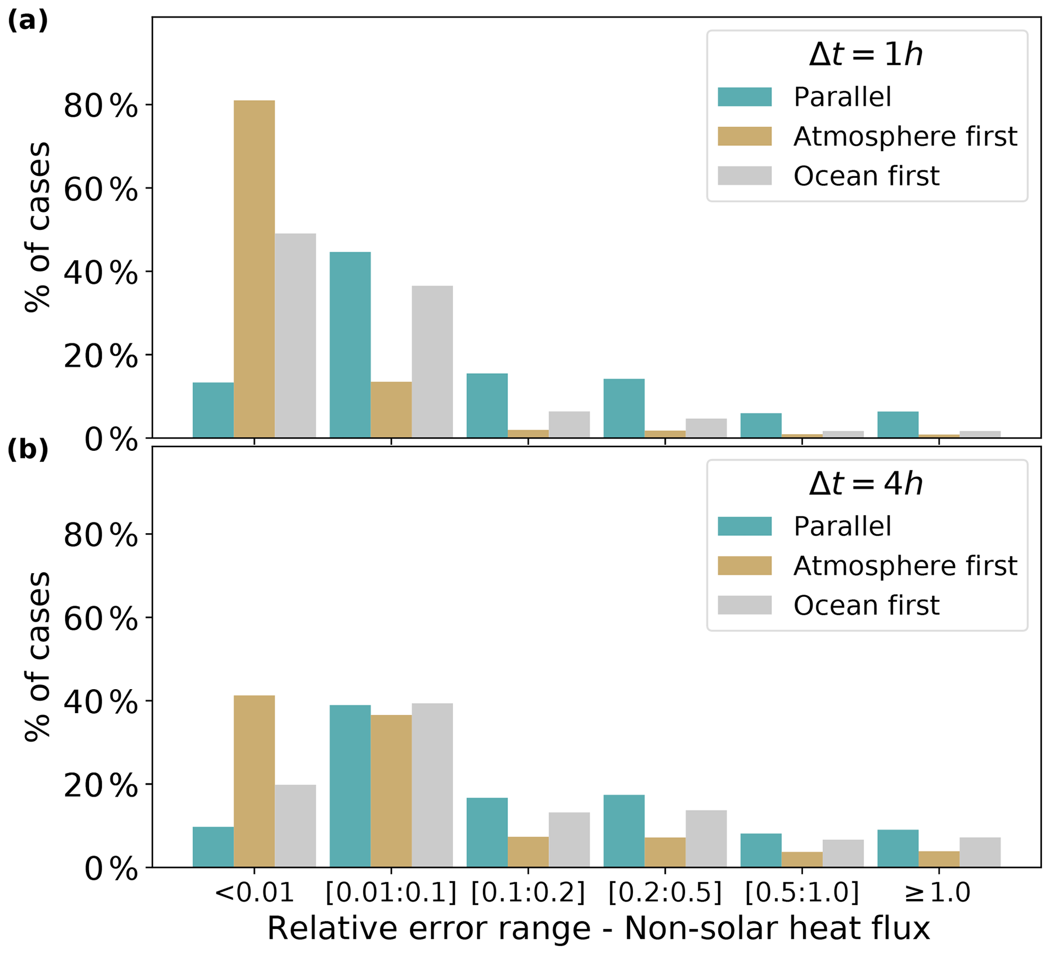
Figure C1Same as Fig. 5, but for the non-solar heat flux, showing the relative error of the change in the non-solar heat flux during a coupling period. The error is computed as the ratio between (i) the correction due to the iterative procedure (the jump from green dots to the converged solution in grey in Fig. 3) and (ii) the solution change between t and t+Δt with no Schwarz iteration (the jump from yellow to green dots in Fig. 3). See the legend in Fig. 4 for the explanation of the x axis.
All code and data relevant to this study are available at https://doi.org/10.5281/zenodo.4546183 (Marti et al., 2020). This digital object identifier (DOI) points to three files. Marti-GMD-2020-307_Models.tar.zip is a gzipped tar file of 218 MB with the model code and scripts needed to run the model (Fortran, C++ and Bash). Marti-GMD-2020-307_Figures.zip is a zip file of 3.3 MB containing the scripts needed to produce the figures: one PyFerret script and seven Jupyter Python notebooks. Marti-GMD-2020-307_Data.tar.zip is a gzipped tar file of 18.5 GB with the model outputs needed to produce the figures.
We give in the following more references for the code used. LMDZ, XIOS, NEMO and ORCHIDEE are released under the terms of the CeCILL license. OASIS-MCT is released under the terms of the Lesser GNU General Public License (LGPL). We used model version IPSLCM6.1.9-LR, which is built from the following model components and utilities (SVN branches and tags).
-
NEMO:
branches/2015/nemo_v3_6_STABLE/NEMOGCM, Tag: 9455 -
ORCA1 config:
trunk/ORCA1_LIM3_PISCES, Tag: 278 -
IPSLCM6:
CONFIG/UNIFORM/v6/IPSLCM6, Tag: 4313 -
ORCHIDEE:
tags/ORCHIDEE_2_0/ORCHIDEE,
Tag: 5661 -
OASIS:
branches/OASIS3-MCT_2.0_branch/oasis3-mct, Tag: 1818 -
IOIPSL:
IOIPSL/tags/v2_2_4/src, Tag: HEAD -
LMDZ:
LMDZ6/branches/IPSLCM6.0.15, Tag: 3427 -
libIGCM:
trunk/libIGCM, Tag: 1478 -
XIOS:
XIOS/branchs/xios-2.5, Tag: 1550
Model documentation is available at https://forge.ipsl.jussieu.fr/igcmg_doc/wiki/Doc (last access: 10 May 2021). The code modifications made in IPSLCM6.1.9-LR to build IPSL-CM6-SW-VLR and implement the Schwarz iterative method are fully documented at https://forge.ipsl.jussieu.fr/cocoa (last access: 10 May 2021).
OM co-designed the study, ran some experiments, made the analysis and wrote the paper with large inputs by FL, SV and EB. SN helped to design the study, made all the coding to implement the Schwarz method, ran some experiments and made some analysis. PB co-designed the study. SV brought her expertise in coupling. FL and EB designed the mathematical framework and brought their expertise in all mathematical aspects.
The authors declare that they have no conflict of interest.
This study is part of the ANR project COCOA (https://anr.fr/Projet-ANR-16-CE01-0007, last access: 10 May 2021). This work was granted access to the HPC resources of TGCC under an allocation made by GENCI (Grand Équipement National de Calcul Intensif, grant 2019-A0040100239). It benefits from the development of the common modeling IPSL infrastructure coordinated by the IPSL climate modeling center (https://cmc.ipsl.fr, last access: 10 May 2021). Data files were prepared with NCO (NetCDF Operators; Zender, 2008, and http://nco.sourceforge.net, last access: 19 May 2021). Sketches are drawn with LibreOffice (https://www.libreoffice.org, last access: 10 May 2021). Plots and histograms are produced with Matplotlib (Hunter, 2007, and https://matplotlib.org, last access: 10 May 2021) in Jupyter Python notebooks. Maps were drawn with pyFerret, a product of NOAA's Pacific Marine Environmental Laboratory (http://ferret.pmel.noaa.gov/Ferret, last access: 10 May 2021). Patrick Brockman and Jean-Yves Peterschmitt brought invaluable help in the realization of the figures. We thank the reviewers for their kind yet helpful reviews: the original paper studied the IPSLCM6 legacy parallel algorithm, and the sequential ones were added from their suggestions.
This research has been supported by the ANR project COCOA (grant no. ANR-16-CE01-0007TS5) and by Grand Équipement National de Calcul Intensif (GENCI, grant no. 2019-A0040100239).
This paper was edited by Qiang Wang and reviewed by Li Liu and Jan Streffing.
Balaji, V., Anderson, J., Held, I., Winton, M., Durachta, J., Malyshev, S., and Stouffer, R. J.: The Exchange Grid, in: Parallel Computational Fluid Dynamics 2005, Elsevier, 179–186, https://doi.org/10.1016/B978-044452206-1/50021-5, 2006. a
Boucher, O., Servonnat, J., Albright, A. L., Aumont, O., Balkanski, Y., Bastrikov, V., Bekki, S., Bonnet, R., Bony, S., Bopp, L., Braconnot, P., Brockmann, P., Cadule, P., Caubel, A., Cheruy, F., Codron, F., Cozic, A., Cugnet, D., D'Andrea, F., Davini, P., Lavergne, C., Denvil, S., Deshayes, J., Devilliers, M., Ducharne, A., Dufresne, J., Dupont, E., Éthé, C., Fairhead, L., Falletti, L., Flavoni, S., Foujols, M., Gardoll, S., Gastineau, G., Ghattas, J., Grandpeix, J., Guenet, B., Guez, E., L., Guilyardi, E., Guimberteau, M., Hauglustaine, D., Hourdin, F., Idelkadi, A., Joussaume, S., Kageyama, M., Khodri, M., Krinner, G., Lebas, N., Levavasseur, G., Lévy, C., Li, L., Lott, F., Lurton, T., Luyssaert, S., Madec, G., Madeleine, J., Maignan, F., Marchand, M., Marti, O., Mellul, L., Meurdesoif, Y., Mignot, J., Musat, I., Ottlé, C., Peylin, P., Planton, Y., Polcher, J., Rio, C., Rochetin, N., Rousset, C., Sepulchre, P., Sima, A., Swingedouw, D., Thiéblemont, R., Traore, A. K., Vancoppenolle, M., Vial, J., Vialard, J., Viovy, N., and Vuichard, N.: Presentation and Evaluation of the IPSL‐CM6A‐LR Climate Model, J. Adv. Model. Earth Syst., 12, e2019MS002010, https://doi.org/10.1029/2019MS002010, 2020. a, b, c, d
Braconnot, P., Marti, O., and Joussaume, S.: Adjustment and feedbacks in a global coupled ocean-atmosphere model, Clim. Dynam., 13, 507–519, https://doi.org/10.1007/s003820050179, 7-8, 1997. a
Connors, J. M. and Ganis, B.: Stability of algorithms for a two domain natural convection problem and observed model uncertainty, Comput. Geosci., 15, 509–527, https://doi.org/10.1007/s10596-010-9219-x, 2011. a
Ducoudré, N. I., Laval, K., and Perrier, A.: SECHIBA, a New Set of Parameterizations of the Hydrologic Exchanges at the Land-Atmosphere Interface within the LMD Atmospheric General Circulation Model, J. Climate, 6, 248–273, https://doi.org/10.1175/1520-0442(1993)006<0248:SANSOP>2.0.CO;2, 1993. a, b, c
Dufresne, J.-L., Foujols, M.-A., Denvil, S., Caubel, A., Marti, O., Aumont, O., Balkanski, Y., Bekki, S., Bellenger, H., Benshila, R., Bony, S., Bopp, L., Braconnot, P., Brockmann, P., Cadule, P., Cheruy, F., Codron, F., Cozic, A., Cugnet, D., Noblet, N., Duvel, J.-P., Ethé, C., Fairhead, L., Fichefet, T., Flavoni, S., Friedlingstein, P., Grandpeix, J.-Y., Guez, L., Guilyardi, E., Hauglustaine, D., Hourdin, F., Idelkadi, A., Ghattas, J., Joussaume, S., Kageyama, M., Krinner, G., Labetoulle, S., Lahellec, A., Lefebvre, M.-P., Lefevre, F., Lévy, C., Li, Z. X., Lloyd, J., Lott, F., Madec, G., Mancip, M., Marchand, M., Masson, S., Meurdesoif, Y., Mignot, J., Musat, I., Parouty, S., Polcher, J., Rio, C., Schulz, M., Swingedouw, D., Szopa, S., Talandier, C., Terray, P., Viovy, N., and Vuichard, N.: Climate change projections using the IPSL-CM5 Earth System Model: from CMIP3 to CMIP5, Clim. Dyn., 40, 2123–2165, https://doi.org/10.1007/s00382-012-1636-1, 2013. a, b, c, d
Eyring, V., Bony, S., Meehl, G. A., Senior, C. A., Stevens, B., Stouffer, R. J., and Taylor, K. E.: Overview of the Coupled Model Intercomparison Project Phase 6 (CMIP6) experimental design and organization, Geosci. Model Dev., 9, 1937–1958, https://doi.org/10.5194/gmd-9-1937-2016, 2016. a
Foken, T.: 50 Years of the Monin–Obukhov Similarity Theory, Boundary-Lay. Meteorol., 119, 431–447, https://doi.org/10.1007/s10546-006-9048-6, 2006. a
Gander, M. J. and Halpern, L.: Optimized Schwarz Waveform Relaxation Methods for Advection Reaction Diffusion Problems, SIAM J. Numer. Anal., 45, 666–697, https://doi.org/10.1137/050642137, 2007. a
Gander, M. J., Halpern, L., and Nataf, F.: Optimal Convergence for Overlapping and Non-Overlapping Schwarz Waveform Relaxation, in: Proceedings of the 11th International Conference on Domain Decomposition Methods, The University of Greenwich, Greenwich, UK, 27–36, available at: https://archive-ouverte.unige.ch/unige:8286 (last access: 10 May 2021), 1999. a
Gross, M., Wan, H., Rasch, P. J., Caldwell, P. M., Williamson, D. L., Klocke, D., Jablonowski, C., Thatcher, D. R., Wood, N., Cullen, M., Beare, B., Willett, M., Lemarié, F., Blayo, E., Malardel, S., Termonia, P., Gassmann, A., Lauritzen, P. H., Johansen, H., Zarzycki, C. M., Sakaguchi, K., and Leung, R.: Physics–Dynamics Coupling in Weather, Climate, and Earth System Models: Challenges and Recent Progress, Mon. Weather Rev., 146, 3505–3544, https://doi.org/10.1175/MWR-D-17-0345.1, 2018. a, b, c
Hunter, J. D.: Matplotlib: A 2D graphics environment, Comput. Sci. Eng., 9, 90–95, https://doi.org/10.1109/MCSE.2007.55, publisher: IEEE Computer Soc., 2007. a
Keyes, D. E., McInnes, L. C., Woodward, C., Gropp, W., Myra, E., Pernice, M., Bell, J., Brown, J., Clo, A., Connors, J., Constantinescu, E., Estep, D., Evans, K., Farhat, C., Hakim, A., Hammond, G., Hansen, G., Hill, J., Isaac, T., Jiao, X., Jordan, K., Kaushik, D., Kaxiras, E., Koniges, A., Lee, K., Lott, A., Lu, Q., Magerlein, J., Maxwell, R., McCourt, M., Mehl, M., Pawlowski, R., Randles, A. P., Reynolds, D., Rivière, B., Rüde, U., Scheibe, T., Shadid, J., Sheehan, B., Shephard, M., Siegel, A., Smith, B., Tang, X., Wilson, C., and Wohlmuth, B.: Multiphysics simulations: Challenges and opportunities, Int. J. High Perform. C., 27, 4–83, https://doi.org/10.1177/1094342012468181, 2013. a
Large, W. B.: Surface Fluxes for Practitioners of Global Ocean Data Assimilation, in: Ocean Weather Forecasting, edited by: Chassignet, E. P. and Verron, J., Springer-Verlag, Berlin/Heidelberg, 229–270, https://doi.org/10.1007/1-4020-4028-8_9, 2006. a
Lemarié, F.: Algorithmes de Schwarz et couplage océan-atmosphère, PhD thesis, Université Joseph Fourier, Grenoble, available at: https://tel.archives-ouvertes.fr/tel-00343501 (last access: 10 May 2021), 2008. a, b, c, d
Lemarié, F., Debreu, L., and Blayo, E.: Toward an Optimized Global-in-Time Schwarz Algorithm for Diffusion Equations with Discontinuous and Spatially Variable Coefficients, Part 1: The Constant Coefficients Case, Electron. T. Numer. Ana., 40, 148–169, 2013. a
Lemarié, F., Marchesiello, P., Debreu, L., and Blayo, E.: Sensitivity of ocean-atmosphere coupled models to the coupling method : example of tropical cyclone Erica, Research Report 8651, INRIA, available at: https://hal.inria.fr/hal-00872496v6/document (last access: 10 May 2021), 2014. a, b, c, d
Lemarié, F., Blayo, E., and Debreu, L.: Analysis of Ocean-atmosphere Coupling Algorithms: Consistency and Stability, Procedia Comput. Sci., 51, 2066–2075, https://doi.org/10.1016/j.procs.2015.05.473, 2015. a, b, c, d
Locarnini, R. A., Mishonov, A. V., Antonov, J. I., Boyer, T. P., Garcia, H. E., Baranova, O. K., Zweng, M. M., Paver, C. R., Reagan, J. R., Johnson, D. R., Hamilton, M., and Seidov, D.: World OceanAtlas 2013, Volume 1: Temperature, edited by: Levitus, S., NOAA Atlas NESDIS 73, NOAA, available at: https://rda.ucar.edu/datasets/ds285.0/docs/woa13/woa13_vol1.pdf (last access: 10 May 2021), 2013. a, b
Marti, O., Braconnot, P., Dufresne, J.-L., Bellier, J., Benshila, R., Bony, S., Brockmann, P., Cadule, P., Caubel, A., Codron, F., de Noblet, N., Denvil, S., Fairhead, L., Fichefet, T., Foujols, M.-A., Friedlingstein, P., Goosse, H., Grandpeix, J.-Y., Guilyardi, E., Hourdin, F., Idelkadi, A., Kageyama, M., Krinner, G., Lévy, C., Madec, G., Mignot, J., Musat, I., Swingedouw, D., and Talandier, C.: Key features of the IPSL ocean atmosphere model and its sensitivity to atmospheric resolution, Clim. Dynam., 34, 1–26, https://doi.org/10.1007/s00382-009-0640-6, 2010. a, b, c
Marti, O., Nguyen, S., Braconnot, P., Valcke, S., Lemarié, F., and Blayo, E.: A Schwarz iterative method to evaluate ocean- atmosphere coupling schemes. Implementation and diagnostics in IPSL-CM6-SW-VLR. GMD-2020-307 [Data set], Geoscientific Model Development, Zenodo, https://doi.org/10.5281/zenodo.4273949, 2020. a
Pelletier, C., Lemarié, F., and Blayo, E.: Sensitivity analysis and metamodels for the bulk parametrization of turbulent air-sea fluxes, Q. J. Roy. Meteor. Soc., 144, 658–669, https://doi.org/10.1002/qj.3233, 2018. a
Rousset, C., Vancoppenolle, M., Madec, G., Fichefet, T., Flavoni, S., Barthélemy, A., Benshila, R., Chanut, J., Levy, C., Masson, S., and Vivier, F.: The Louvain-La-Neuve sea ice model LIM3.6: global and regional capabilities, Geosci. Model Dev., 8, 2991–3005, https://doi.org/10.5194/gmd-8-2991-2015, 2015. a, b
Sepulchre, P., Caubel, A., Ladant, J.-B., Bopp, L., Boucher, O., Braconnot, P., Brockmann, P., Cozic, A., Donnadieu, Y., Dufresne, J.-L., Estella-Perez, V., Ethé, C., Fluteau, F., Foujols, M.-A., Gastineau, G., Ghattas, J., Hauglustaine, D., Hourdin, F., Kageyama, M., Khodri, M., Marti, O., Meurdesoif, Y., Mignot, J., Sarr, A.-C., Servonnat, J., Swingedouw, D., Szopa, S., and Tardif, D.: IPSL-CM5A2 – an Earth system model designed for multi-millennial climate simulations, Geosci. Model Dev., 13, 3011–3053, https://doi.org/10.5194/gmd-13-3011-2020, 2020. a, b, c, d, e, f, g, h, i
Thery, S., Pelletier, C., Lemarié, F., and Blayo, E.: Analysis of Schwarz Waveform Relaxation for the Coupled Ekman Boundary Layer Problem with Continuously Variable Coefficients, available at: https://hal.inria.fr/hal-02544113 (last access: 10 May 2021), 2020. a, b
Wikipedia: Roman timekeeping, available at: https://en.wikipedia.org/w/index.php?title=Roman_timekeeping&oldid=990684875 (last access: 10 May 2021), 2020. a
Zender, C. S.: Analysis of self-describing gridded geoscience data with netCDF Operators (NCO), Environ. Model. Softw., 23, 1338–1342, https://doi.org/10.1016/j.envsoft.2008.03.004, 2008. a
The terms “synchronous” and “asynchronous” may have a totally different signification for climate modelers, and we prefer to avoid them.
- Abstract
- Introduction
- State-of-the-art ocean–atmosphere coupling algorithms and the Schwarz method
- Model and experiments
- Results
- Conclusions and future approaches
- Appendix A: Evaluation of IPSL-CM6-SW-VLR
- Appendix B: Algorithms
- Appendix C: Are conclusions drawn from sea surface temperature robust?
- Code and data availability
- Author contributions
- Competing interests
- Acknowledgements
- Financial support
- Review statement
- References