Unstructured global to coastal wave modeling for the Energy Exascale Earth System Model using WAVEWATCH III version 6.07

Wind-wave processes have generally been excluded from coupled Earth system models due to the high computational expense of spectral wave models, which resolve a frequency and direction spectrum of waves across space and time. Existing uniform-resolution wave modeling approaches used in Earth system models cannot appropriately represent wave climates from global to coastal ocean scales, largely because of tradeoffs between coastal resolution and computational costs. To resolve this challenge, we introduce a global unstructured mesh capability for the WAVEWATCH III (WW3) model that is suitable for coupling within the US Department of Energy's Energy Exascale Earth System Model (E3SM). The new unstructured WW3 global wave modeling approach can provide the accuracy of higher global resolutions in coastal areas at the relative cost of lower uniform global resolutions. This new capability enables simulation of waves at physically relevant scales as needed for coastal applications.

1 Introduction

Wind-generated waves play an important interfacial role in the global coupled climate system. They mediate multi-phase interactions between the ocean, atmosphere, and sea ice (Cavaleri et al., 2012) and influence the land surface in coastal zones (Mariotti and Fagherazzi, 2010). For example, wave processes drive air–sea momentum transfer (Donelan et al., 2012), enhance ocean mixing via Langmuir turbulence (Belcher et al., 2012), and modulate ocean surface albedo (Frouin et al., 2001). Ocean currents also interact with waves via Doppler shifting, which has an effect on wave heights (Ardhuin et al., 2017). Wave physics are also critical drivers of coastal processes such as wave setup (Longuet-Higgins and Stewart, 1964), which affects coastal flooding (Dietrich et al., 2011) and sediment transport (Warner et al., 2010). In high-latitude regions, sea ice damps wave propagation, and in turn, waves fracture ice floes in the marginal ice zone (Squire et al., 1995). Waves also drive unstable currents at the ice edge, leading to mesoscale eddy generation (Dai et al., 2019).

In all of these coupled Earth system model applications, high mesh resolution is required to accurately model waves in coastal regions, largely due to the role waves play at these interfacial scales. As shown in Fig. 1, wind wave periods represent a distinct portion of the energy spectrum that would be infeasible to resolve explicitly. Phase-resolving wave models (Kennedy et al., 2000), although necessary for applications such as coastal engineering, e.g., harbor design, are too expensive for use beyond local coastal areas. Phase-averaged approaches are applicable and appropriate for larger-scale applications because they do not directly resolve the free surface. However, even phase-averaged spectral wave models are quite expensive compared to the atmospheric and oceanic dynamic cores used in Earth system models.

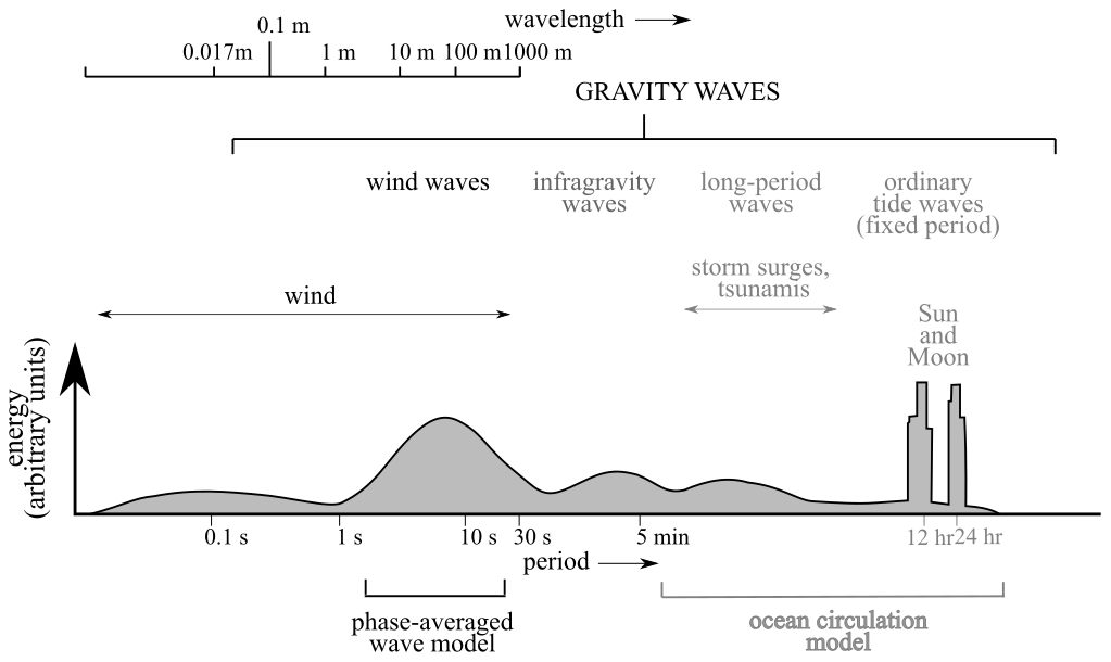
Figure 1 Energy spectrum for wave frequencies in the ocean showing the role of phase-averaged spectral wave models. Adapted from Wright et al. (1999).

Since phase-averaged spectral wave models are known to be expensive, variable-resolution approaches can be used to economically resolve both the coastal and global regimes. Using uniform structured meshes, the resolution will either be too coarse to accurately simulate coastal waves or the computational cost will be too great to resolve the entire global ocean. Unstructured capabilities, however, provide the flexibility to resolve key scales relevant to accurate wave simulation in coastal regions, e.g., shallow wave breaking as a function of water depth, shoaling, refraction, and triad wave interactions (Zijlema, 2010).

Ultimately, waves must be simulated in Earth system models because the historical wave climate is evolving under decadal-scale climate changes. The global wave climate has become increasingly intense as driven by increased wind speeds (Young et al., 2011) and warming sea surface temperatures (Reguero et al., 2019). This trend is expected to increase under future greenhouse gas emission scenarios (Hemer et al., 2013; Amores and Marcos, 2020). This has important implications for assessing the impacts of climate change in coastal regions. The combination of sea level rise and more intense storms will make coastal inundation from storm surge and waves a bigger risk to coastal communities (Vousdoukas et al., 2018). A more extreme wave climate will also continue to drive coastline changes (Mentaschi et al., 2018). Furthermore, waves are also a potential source of renewable energy. Modeling the future wave climate is important to designing effective wave energy conversion strategies (Wu et al., 2020).

Increased wave climate intensity also has consequences for high-latitude regions. Longer fetch lengths due to decreasing sea ice extent in the Arctic produce larger long period waves that are more effective at fracturing sea ice. This has the potential to cause a feedback in which waves accelerate sea ice retreat, leading to yet longer fetch lengths (Thomson and Rogers, 2014). The loss of sea ice also increases the exposure of Antarctic ice shelves to swell waves, which can lead to calving (Massom et al., 2018) and contribute to sea level rise. In addition, increased wave energy paired with sea ice and permafrost loss in the Arctic could also be responsible for increased coastal erosion rates in the region (Overeem et al., 2011).

Addressing science questions related to these risks will require a variable-resolution wave modeling approach. To date, global wave modeling has primarily been performed using uniform structured meshes or nested structured meshes. Unstructured triangular meshes have traditionally been limited to regional coastal applications. However, a long-term promise of unstructured approaches is the capability to span small to large scales across the coastal to global ocean. The purpose of this paper is to report on progress toward this goal, starting with an assessment of the accuracy and performance of the WAVEWATCH III (WW3) model (Tolman, 1991) using global to coastal unstructured meshes, which are compared to a single structured grid. These meshes will allow wave simulations to maintain accuracy across the global and coastal oceans at reduced computational cost. This creates an opportunity to represent the effects of waves across a broad spectrum of coupled interactions within Earth system models.

The remainder of the paper is organized as follows. First, a background of variable-resolution wave modeling is presented in Sect. 2. Second, we describe the unstructured mesh configuration we have developed for WW3 and the comparison study used to assess its accuracy and performance (Sect. 3). Then, the accuracy of the unstructured mesh is compared against high- and low-resolution structured meshes and measured data from buoy observations (Sect. 4.1 and 4.2). Next, we demonstrate the computational performance of the unstructured mesh alongside that of the structured meshes (Sect. 4.3). We also discuss the results in the context of developing efficient coastal Earth system models (Sect. 5). Ultimately, we conclude that unstructured WW3 is a viable means of exploring wave interactions within coastal Earth system model applications for the US Department of Energy's Energy Exascale Earth System Model (E3SM) (Sect. 6).

2 WW3 multi-resolution approaches

In this work, we analyze wave simulation accuracy and performance across the global to coastal ocean using version 6.07 of WW3 (WAVEWATCH III® Development Group, 2019). WW3 is a third-generation spectral wave model that has been used widely for operational wave forecasting, research, and engineering applications (Chawla et al., 2013b; Alves et al., 2014; Cornett, 2008; Wang and Oey, 2008). Similar models include the WAve Model (WAM) (WAMDI Group, 1988) and the Simulating WAves Nearshore (SWAN) (Booij et al., 1999) coastal wave model. These phase-averaged spectral wave models describe the evolution of the wave action density spectrum, $N(\mathit{\lambda },\mathit{\varphi },k,\mathit{\theta },t)$, which is a function of both longitude–latitude (λ,ϕ) and wavenumber–direction (k,θ) space. The action density spectrum is related to the energy spectrum, F, by the intrinsic frequency, σ, that is observed moving with the current:

$$\begin{array}{}\text{(1)}& N(k,\mathit{\theta })={\displaystyle \frac{F(k,\mathit{\theta })}{\mathit{\sigma }}}.\end{array}$$

As opposed to wave energy, action density is conserved generally in the presence of ocean currents (Whitham, 1965; Bretherton and Garrett, 1968). The intrinsic frequency is given by the dispersion relationship from linear wave theory:

$$\begin{array}{}\text{(2)}& \mathit{\sigma }=\sqrt{gk\tanh \left(kd\right)},\end{array}$$

where d is the depth, k is the wavenumber, and g is the acceleration due to gravity. The evolution of the wave action density is described by the following equation:

$$\begin{array}{}\text{(3)}& {\displaystyle \frac{\partial N}{\partial t}}+{\displaystyle \frac{\mathrm{1}}{\cos \mathit{\varphi }}}{\displaystyle \frac{\partial }{\partial \mathit{\varphi }}}\left(\dot{\mathit{\varphi }}N\cos \mathit{\varphi }\right)+{\displaystyle \frac{\partial }{\partial \mathit{\lambda }}}\left(\dot{\mathit{\lambda }}N\right)+{\displaystyle \frac{\partial }{\partial k}}\left(\dot{k}N\right)+{\displaystyle \frac{\partial }{\partial \mathit{\theta }}}\left(\dot{\mathit{\theta }}N\right)={\displaystyle \frac{S}{\mathit{\sigma }}},\end{array}$$

where $\dot{\mathit{\varphi }}$, $\dot{\mathit{\lambda }}$, $\dot{k}$, and $\dot{\mathit{\theta }}$ are the propagation velocities in geographic and spectral space. These propagation velocities are functions of the group velocity, ocean currents, and derivatives of σ with respect to direction. The S term on the right-hand side of Eq. (3) is comprised of parameterized source–sink terms that represent several wave processes, i.e.,

$$\begin{array}{}\text{(4)}& S=S_{\mathrm{in}}+S_{\mathrm{ds}}+S_{\mathrm{nl}}+S_{\mathrm{bot}}+S_{\mathrm{db}}+\mathrm{\dots }.\end{array}$$

These source–sink terms describe: generation due to wind (S_in), dissipation (S_ds), non-linear quadruplet interactions (S_nl), bottom friction (S_bot), and depth-limited breaking (S_db). There are several other parameterizations that can be included (e.g., sea ice damping, triad interactions, coastline reflection) but these are the primary terms relevant to this work.

Equation (3) requires discretization of the left-hand side transport terms for numerical simulations. Traditionally, structured meshes have been employed due to the straightforward application of numerical methods and for computational simplicity (WAMDI Group, 1988). However, coastal simulations require advanced approaches. Three primary options have been developed in WW3 to address the need for variable resolution: two-way nested “mosaic” grids (Tolman, 2008), spherical multi-cell (SMC) grids (Li, 2012), and regional triangular unstructured meshes (Roland, 2008).

2.1 Nested and multi-cell meshes

The two-way nested mosaic approach has been extensively validated against historical wave observations and is used for NOAA forecasting operations (Chawla et al., 2013a). However, two-way nesting of structured meshes has several disadvantages (Zijlema, 2010). In these types of meshes, transitions in resolution are typically abrupt. Therefore, they must either be placed well outside regions where high resolution is needed in order to be accurate, or a series of nested meshes must be employed to achieve a smooth transition. This means high-resolution regions must be larger than necessary to avoid degrading accuracy or increasing the complexity of the nested model. Two-way nesting also requires a sufficient overlap region, which means duplicate calculations are performed in these regions on both the coarse and fine meshes. SMC grids provide an alternative multi-resolution capability. However, similar to nested meshes, SMC meshes also lack the ability to smoothly vary resolution in a flexible manner. Another option is to nest an unstructured coastal wave model, such as SWAN (Zijlema, 2010), inside a global WW3 domain (Amrutha et al., 2016). However, this approach uses the WW3 wave spectrum solution to force the boundary of the nested SWAN model, which only provides a one-way coupling between the models. For coupled E3SM applications, two-way feedbacks between the coastal to the global ocean within the wave model are desired.

2.2 Triangular meshes

The previously mentioned approaches are disadvantageous for Earth system modeling because field remapping approaches are needed to facilitate coupling between Earth system model components (Jones, 1999; Ullrich and Taylor, 2015). Field remapping for these types of meshes is complicated, more computationally expensive, and historically has not been employed in production Earth system simulations. Mosaic grids and WW3/SWAN nesting may be appropriate for specific regional domains and wave modeling efforts. However, they are not considered here due to their added complexity and heterogeneity for E3SM applications.

In contrast, the primary advantages of triangular grids are their flexibility and ability to transition resolution smoothly between different regions of the mesh. They also offer a more straightforward integration into coupled Earth system model applications. To date, unstructured meshes have been primarily used in regional studies to assess accuracy in coastal settings (Roland and Ardhuin, 2014; Abdolali et al., 2020; Dietrich et al., 2011). But, a detailed global assessment of deep to shallow water accuracy with mesh refinement in coastal areas has not yet been performed.

The goal of this paper is to evaluate the potential for wave simulation approaches in Earth system models by demonstrating that coastal unstructured meshes can be extended to global domains in order to efficiently simulate the wave climate across the global and coastal ocean, from deep to shallow water. The importance of this global unstructured capability is growing as Earth system models, e.g., E3SM (Golaz et al., 2019), are beginning to use a multi-resolution approach to understand regional climate change impacts. Efforts to include waves into the Community Earth System Model (CESM) using structured meshes (Li et al., 2016) have used very coarse (3.2 × 4^∘) resolution in order to keep the computational cost reasonable. This resolution simulated the wave climate well enough to improve mixed layer depth biases in the global ocean. However, higher mesh resolution is necessary to accurately describe coastal or high-latitude wave dynamics. This is something that is not currently possible in structured Earth system models like CESM.

3 Methods

This section outlines the unstructured mesh, model configuration, and treatment of unresolved islands used in the validation study. It also gives a description of the simulation performed and the metrics used to assess the accuracy of the unstructured mesh results.

3.1 Global unstructured mesh

The unstructured mesh developed for this comparison study is designed to maintain the global and coastal accuracy of high-resolution structured WW3 simulations at reduced computational expense. The coastal resolution is specified based on a simple depth criterion. In this mesh, the refined resolution has been limited to US coastlines in accordance with current E3SM simulation campaign goals, e.g., as partially outlined in Hoch et al. (2020).

The mesh used in this study was generated using the OceanMesh2D software package (Roberts et al., 2019), which has shoreline resolving capabilities. Future applications will use the JIGSAW mesh generator (Engwirda, 2017) once shoreline-resolving capabilities are developed for global meshes. This will allow for the same mesh generation tools to be used across the ocean, sea ice, and wave components of E3SM. Globally, the mesh has 2^∘ resolution and transitions to 0.5^∘ resolution in regions where the depth is less than 4000 m, as illustrated in Fig. 2. Since changes in depth play an important role in the evolution of the wave field, this 4000 m depth criterion has been chosen to ensure that the steep transitions from deep ocean to coastal regions and shallow inner seas are resolved (Cavaleri et al., 2018). Since depth effects on waves become important on the continental shelf, the 4000 m value allows this transition region to be resolved, while not introducing extra resolution in the deep ocean. A 10 % element size grade is enforced in the transition region between the 2 and 0.5^∘ resolutions.

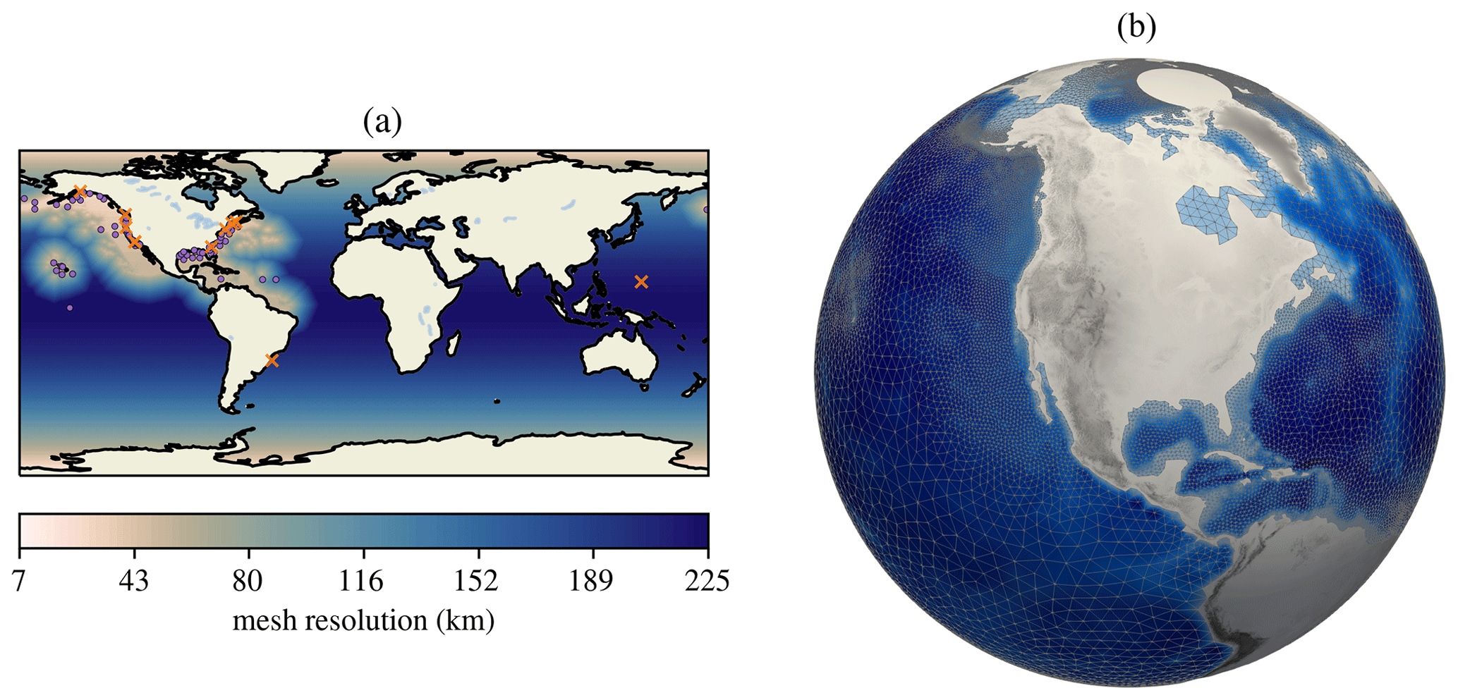
Figure 2 Unstructured mesh with global 2^∘ resolution and 0.5^∘ resolution in regions with depths of less than 4 km within the coastal US: (a) quantitative mesh resolution and (b) qualitative mesh resolution and bathymetry. In panel (a), dots indicate stations used in the validation, while X indicates those excluded as explained in Sect. 3.6.

The WW3 source code required minor modifications in order to enforce the periodicity of the mesh across the dateline. This minimal change corrected the edge length and area calculations for elements that straddle the −180–+180^∘ boundary.

3.2 Mesh comparisons

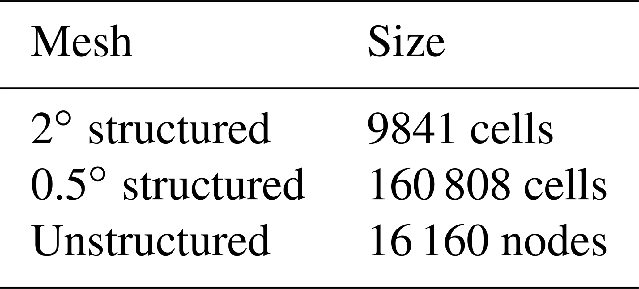
To validate and assess the performance of the global unstructured mesh in WW3, we have performed a study that demonstrates the accuracy and efficiency of using unstructured meshes for global applications. This was done by comparing the unstructured mesh described in Sect. 3.1 with 2 and 0.5^∘ structured meshes. The size of these meshes in terms of structured grid cells and unstructured mesh nodes can be found in Table 1. Both of the structured meshes were generated using the software developed by the NOAA WW3 development team (Chawla and Tolman, 2007). The structured meshes have been cropped at 82^∘ north due to Courant–Friedrichs–Lewy (CFL) condition constraints caused by converging lines of latitude near the pole, similar to those used for NOAA operational modeling (Chawla et al., 2013a). For consistency of comparisons, this was also done in the unstructured mesh in Fig. 2b.

As we will show in the next section, the 2 and 0.5^∘ structured meshes provide roughly equivalent levels of accuracy in the deep ocean. However, as expected, the 0.5^∘ structured mesh far outperforms the 2^∘ mesh in shallow coastal regions. Simulating nearshore wave dynamics with a high level of accuracy would require finer than 0.5^∘ mesh resolution (Dietrich et al., 2011; Perez et al., 2017; Abdolali et al., 2020; Chawla et al., 2013a). However, we have chosen 0.5^∘ as our highest resolution since it performs reasonably well at our validation stations, and we are targeting resolutions that would be economically viable for global climate modeling applications. Note that for explicit time integration, time step restrictions due to the CFL condition for the highest-resolution elements impact the overall computational time required for climate evaluations.

Table 1 Mesh sizes considered in this study.

The goal of this comparison is to demonstrate that the unstructured mesh is able to match the deep ocean accuracy of the structured meshes, while providing equivalent accuracy to the structured 0.5^∘ mesh in the refined coastal regions. Due to having coarse resolution over most of the globe, the unstructured mesh is expected to be more computationally efficient than the global 0.5^∘ structured mesh.

3.3 Simulation forcing

Each of the three meshes is used to perform a wave hindcast from the beginning of June 2005 to the end of October 2005. This time period represents the 2005 Atlantic hurricane season, which is the most intense hurricane season on record (Beven et al., 2008). For the unstructured mesh, this is also a challenging time period because strong seasonal swell from the Southern Ocean during these months (Young, 1999) is generated in coarse regions of the mesh and propagates into the refined region. Since wind-wave dynamics represent a damped system forced by atmospheric winds, i.e., they have a short memory response, long hindcast periods are of lesser importance for validation purposes. The model is forced using winds from the Climate Forecast System Reanalysis (CFSR) (Saha et al., 2010) at 0.5^∘ spatial resolution and hourly time intervals. In this study, no sea ice concentration or ocean reanalysis data are used in the simulations. The bathymetry dataset for all three meshes is the ETOPO1 bathymetry product (Amante and Eakins, 2009), with global coverage and sufficient resolution to represent islands.

3.4 Model configuration

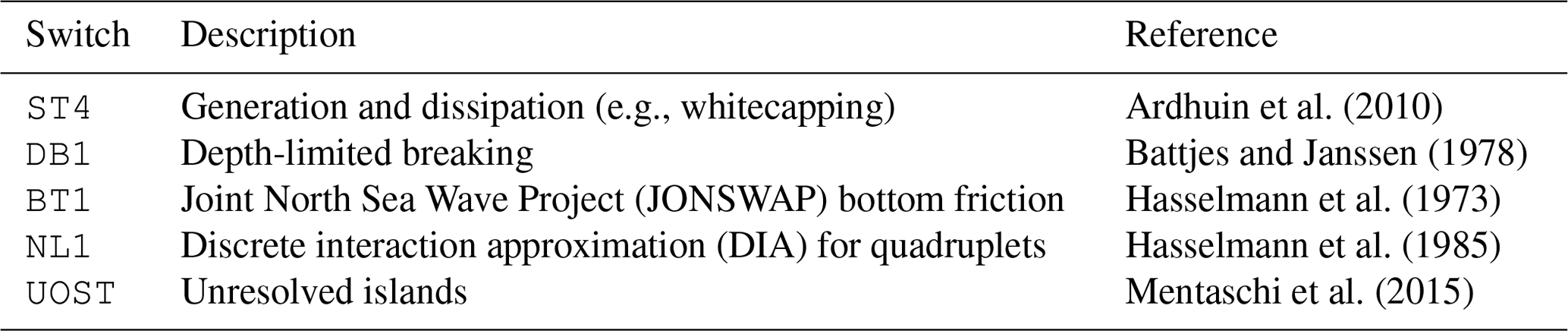
The source–sink term combinations from Eq. (4) can be selected in WW3 using different model “switches”. The options used for both the structured and unstructured mesh simulations are shown in Table 2. We use the ST4 source terms by Ardhuin et al. (2010) since they have been shown to have lower significant wave height biases as compared to other source term packages (Stopa et al., 2016). The default model ST4 values are used with a β_max value of 1.43. This corresponds to the TEST471 values from the WW3 user manual (WAVEWATCH III® Development Group, 2019). Standard approaches are used for bottom friction, non-linear quadruplet interactions, and depth-limited breaking (Chawla et al., 2013a). As discussed in the next section, we also include an unresolved island source term approach instead of the discretization-level correction commonly used in structured mesh WW3 studies (Tolman, 2003). For each of the switches mentioned, we have used their default parameter settings.

Ardhuin et al. (2010)Battjes and Janssen (1978)Hasselmann et al. (1973)Hasselmann et al. (1985)Mentaschi et al. (2015)

Table 2 WW3 physics switches used.

The spectral grid is the same as used in Chawla et al. (2013a). It consists of 36 directions and 50 frequencies with a frequency range of 0.036–0.963 Hz (corresponding to a frequency interval of 1.07). The same spectral mesh is used across all geographic meshes considered.

In order to be consistent across the structured and unstructured meshes, the standard explicit fractional time-stepping scheme is used. The maximum time steps are as follows: 900 s global, 300 s geographic, and 450 s spectral. The minimum source term time step is 30 s. This set of time steps is used for all geographic meshes and is consistent with the finest resolutions used. An implicit method is available for unstructured meshes, but it is not considered here.

Typically, the third-order ULTIMATE QUICKEST scheme (PR3 and UQ switches) is used for the structured mesh discretization. However, the first-order PR1 propagation scheme is used for the structured meshes in this study in order to make a fair comparison against the first-order conservative contour integral-based residual distribution (CRD-N) scheme used for the unstructured mesh (Roland, 2008).

3.5 Unresolved islands

One of the key sources of error in global wave models is the missing dissipation due to unresolved islands. Two different approaches have been developed to include these subgrid-scale effects. The first is implemented as a correction factor to the numerical flux between cells in the propagation scheme (Tolman, 2003). The correction factors are calculated based on the fraction of a cell that is obstructed by an island. This approach is specific to the structured grid propagation schemes in WW3 and has not been generalized to unstructured grids.

The second approach is based on a source term that accounts for the effects of unresolved islands (Mentaschi et al., 2015). This source term considers both the local dissipation and the shadow effect of upstream cells. One advantage of this approach is that it can be used for both structured and unstructured grids. The coefficients required for this source term can be calculated using the open-source Python package alphaBetaLab (Mentaschi et al., 2019).

In our validation and analysis, we have used the source term approach for both the structured and unstructured model configurations, and we focus on accuracy in shallow coastal regions. Not only has the source term parameterization been shown to be slightly more accurate for the structured meshes, but it also allows for a consistent approach across the unstructured and structured simulations (Mentaschi et al., 2018). Thus, differences between results are due to the use of a structured or unstructured mesh and grid resolution. All other factors have been kept constant to make direct comparisons between results to within minor interpolation errors.

3.6 Buoy validation dataset

Validation is performed using best available datasets and community-accepted approaches. Altimeter-based validation has already been presented for global unstructured meshes in WW3 (Mentaschi et al., 2020) and is therefore not repeated here. Instead, we make direct comparisons against available buoy data that span the global and coastal ocean. Buoy data are commonly used to directly quantify the accuracy of spectral wave models, especially for coastal areas. Large-scale systematic biases, which may not necessarily be quantified via sparse and regional buoy data, are assessed against the 0.5^∘ structured mesh that has already been validated for the global ocean (Chawla et al., 2013a). Validation protocols are detailed below.

In Sect. 4.1, data from each of the three meshes are compared with significant wave height data measured by buoys from the National Data Buoy Center (NDBC) (Meindl and Hamilton, 1992), between June–October 2005 and shown at the locations in Fig. 2a. These buoys give an hourly time history of significant wave height, dominant wave period, peak frequency, wind speed, and wind direction. All active buoys from this time period have been used in this analysis, except for 11 out of 115 buoys that either experienced instrument failures or were outside the primary study region. The stations that have been used (∘) and those that were excluded (×) are shown in Fig. 2a. We have focused on significant wave height because it provides the largest dataset across the buoy measurements, compared to frequency and direction observations that are more difficult to observe accurately (Steele et al., 1998). In our analysis, we exclude the first week of the simulation to account for the spin-up period.

3.7 Validation metrics

We use several different metrics to assess the errors between our modeled results and the buoy observations. The first is the commonly used root mean square error (RMSE) defined as

$$\begin{array}{}\text{(5)}& \mathrm{RMSE}=\sqrt{{\displaystyle \frac{\mathrm{1}}{N}}\sum _{i=\mathrm{1}}^N(M_i-O_i{)}^{\mathrm{2}}},\end{array}$$

where M_i is the modeled result, O_i is the observed value, and N is the number of observations. We also show distributions of the bias error:

$$\begin{array}{}\text{(6)}& e_i=M_i-O_i,i=\mathrm{1},\mathrm{\dots },N,\end{array}$$

and relative (normalized bias) error:

$$\begin{array}{}\text{(7)}& {\mathit{\delta }}_i={\displaystyle \frac{M_i-O_i}{O_i}},i=\mathrm{1},\mathrm{\dots },N.\end{array}$$

These error distributions are plotted by binning each e_i and δ_i value throughout the simulation. The counts are then normalized to account for differences in temporal observational coverage for each station. Presenting the errors in this way gives a richer description of the accuracy of a given model than averaged error quantities that can misrepresent skewed biases.

In Sect. 4.2, we also compute average solution differences against the structured 0.5^∘ mesh over the entire global domain to access spatial solution variability due to resolution. These differences are computed by interpolating the unstructured and 2^∘ structured solutions onto the 0.5^∘ mesh. The average and maximum of the e_i and δ_i values are computed from global 3-hourly significant wave height model output.

4 Results

In this section, we describe the results of our validation with buoy data and show global differences between the 0.5^∘ structured mesh and the 2^∘ structured and unstructured meshes. We also give an assessment of computational performance.

4.1 Buoy data validation

Significant wave height error comparisons are shown in Figs. 3–10. Each of these figures represents a different set of stations based on geographical location. For each region, panel (a) shows the RMSE for the station locations in panel (b). The normalized distribution of the error and relative error for each station can be found in panels (c) and (d), respectively.

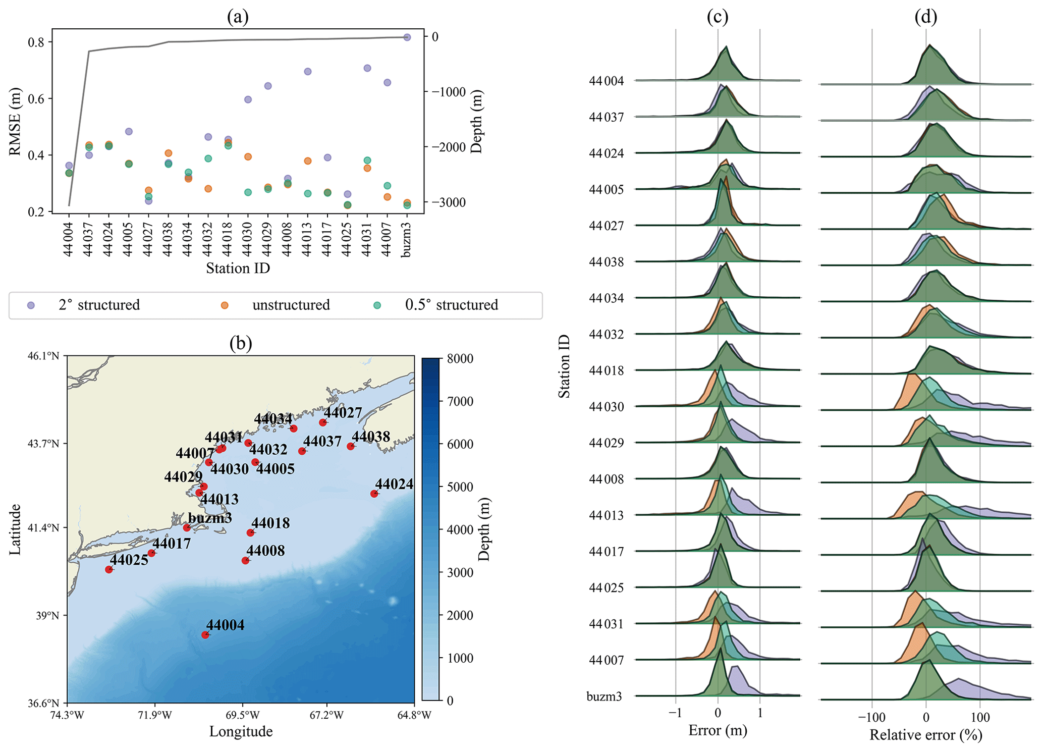
Figure 3 Comparison between modeled results and NDBC buoy data for the 2^∘ structured, unstructured, and 0.5^∘ structured meshes in the Gulf of Maine region. (a) Root mean squared errors (dots) for each mesh resolution along with station depth (gray line). (b) Geographic location of each station. (c) Normalized distribution of bias errors between the model and observations over the simulated time period. (d) Normalized distribution of relative errors.

Comparing the error and relative error distributions can reveal whether the largest errors occur at the largest or smallest observed wave height conditions. If the error distribution becomes more peaked, i.e., the tails are eliminated in the relative error distribution, the largest errors occur at large observed wave heights. In the opposite case, i.e., the error distribution is more diffused compared to the relative error distribution, the larger errors occur during smaller observed wave heights.

In each figure, the station depths are sorted from deep to shallow to depict accuracy differences at varying ocean depths and mesh resolutions. Generally, in the deep ocean, all mesh resolutions provide the same solution accuracy as implied by Li et al. (2016). However, in shallow coastal areas, the high resolution provided by the 0.5^∘ structured and unstructured meshes is necessary to maintain the same accuracy level obtained for the deep ocean.

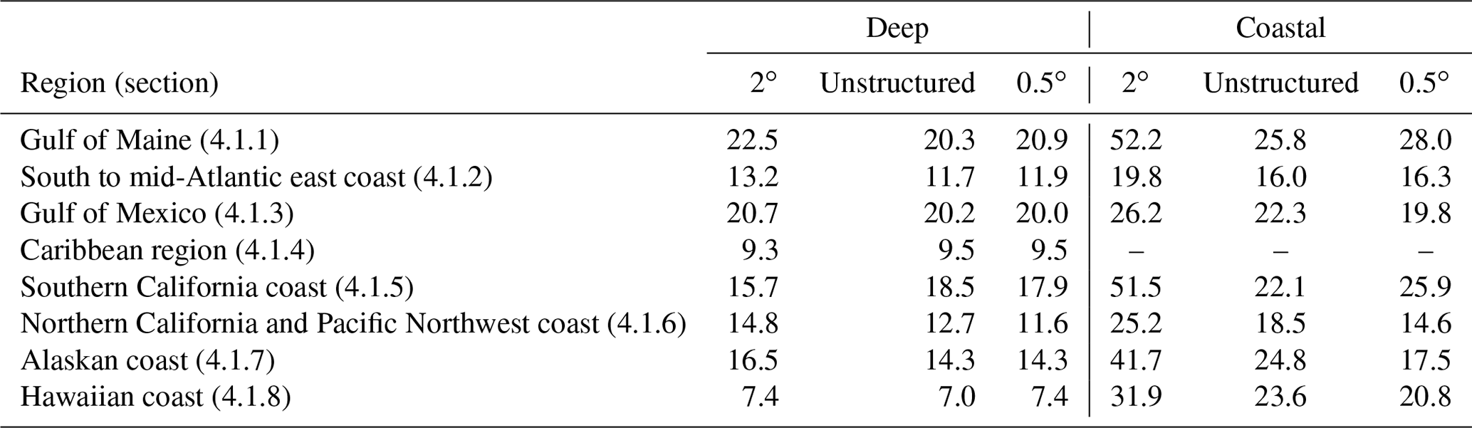
Quantitative evaluations of significant wave heights are presented corresponding to the wave buoys in eight different regions. These include the Gulf of Maine (Sect. 4.1.1), southern to mid-Atlantic east coast (Sect. 4.1.2), Gulf of Mexico (Sect. 4.1.3), Caribbean region (Sect. 4.1.4), Southern California coast (Sect. 4.1.5), Northern California and Pacific Northwest coast (Sect. 4.1.6), Alaskan coast (Sect. 4.1.7), and Hawaiian coast (Sect. 4.1.8). A summary of the relative errors for the three meshes across the deep and shallow buoys in these regions can be found in Table 3, which broadly summarizes the success of the unstructured mesh for both deep and shallow ocean wave simulation. A more detailed analysis for each region is detailed in the following subsections.

Table 3 Comparison of average absolute relative errors (%) between deep (depth > than 1000 m) and coastal (depth ≤ 1000 m) stations for each mesh. The regions shown correspond to those found in Figs. 3–10.

4.1.1 Gulf of Maine

In Fig. 3, the unstructured mesh is of comparable accuracy to the 2 and 0.5^∘ grids for stations 44004–44034 on the x axis of panel (a). The unstructured mesh is more accurate than both of the structured meshes at station 44032. For stations 44030–buzm3, the unstructured mesh provides substantial accuracy improvements over the 2^∘ mesh and its quality approaches 0.5^∘ results, albeit with smaller amplitudes for some buoy locations. The exceptions in this range are stations 44008 and 44025, which are shallow stations where all models provide similar accuracy.

4.1.2 South to mid-Atlantic east coast

Further south of this region, Fig. 4 shows that the unstructured mesh solution generally achieves similar accuracy to the 0.5^∘ structured grid and improves upon the 2^∘ structured grid. The fidelity of the shelf break representation likely plays a role in the accuracy of the unstructured mesh solution, as exemplified by stations 44014 and 41025. The unstructured mesh provides the most accurate result at station 44014 but does not improve as drastically over the 2^∘ solution at a similarly placed shelf-break station to the south, at station 41025. This could be because the mesh happens to more accurately represent the shelf break near station 44014 compared to 41025.

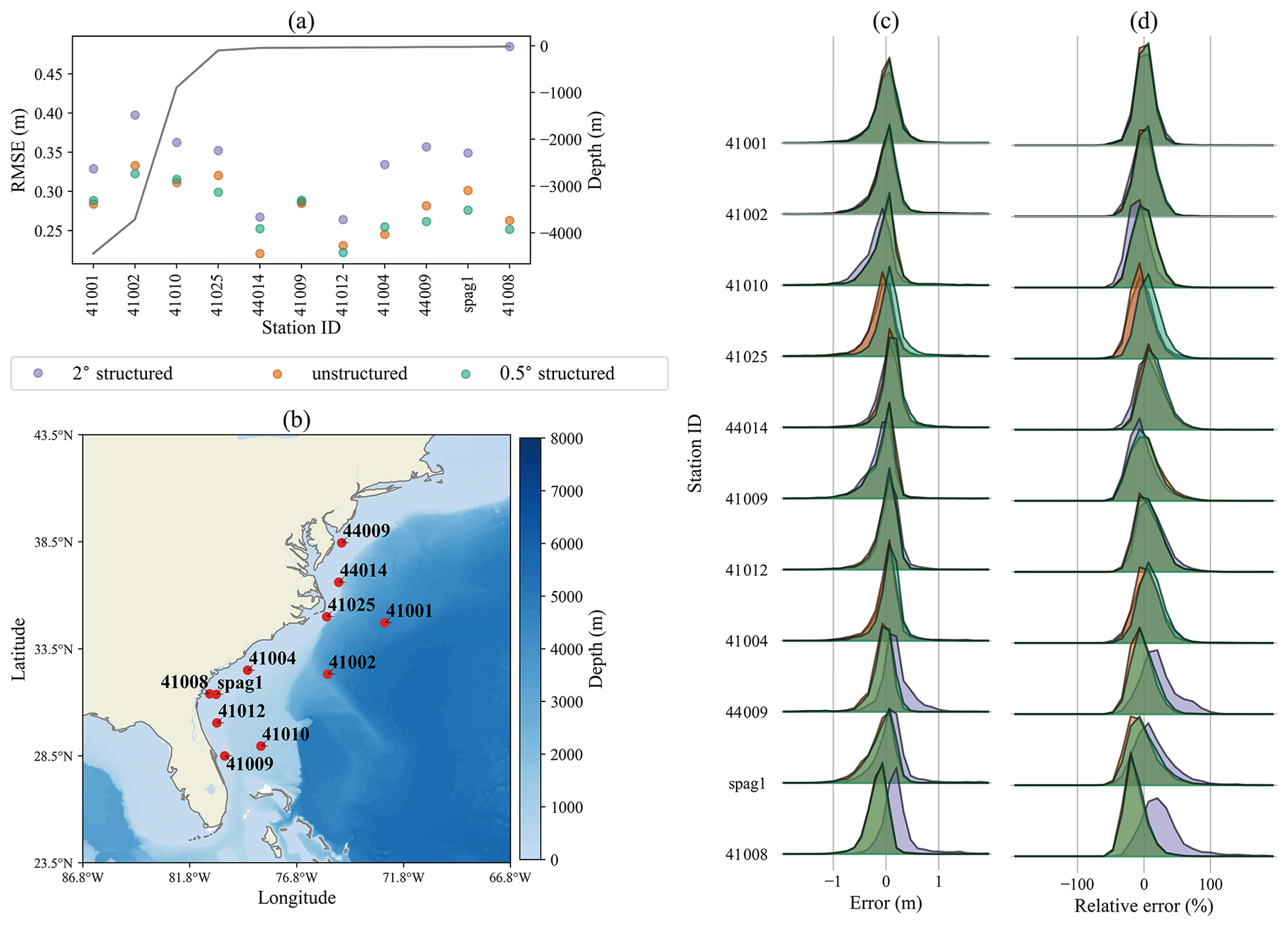
Figure 4 Same as Fig. 3 for stations in the southern to mid-Atlantic east coast.

4.1.3 Gulf of Mexico

In the Gulf of Mexico, shown in Fig. 5, the unstructured and 0.5^∘ results agree well and improve upon the 2^∘ solution for all but one station. The biggest improvement for the unstructured mesh over the 2^∘ mesh is at station 42035, where the 2^∘ mesh is the most inaccurate. The worst station for the unstructured mesh is 42007. This occurs because the unstructured mesh begins to resolve the “bird's foot” portion of the Mississippi River Delta, shielding the wave energy at this station. Throughout the Gulf of Mexico, the unstructured mesh has nearly uniform 0.5^∘ resolution, illustrating parity between the 0.5^∘ structured and 0.5^∘ unstructured approaches. Furthermore, waves in this region are locally generated within the gulf. Therefore, good agreement between the unstructured and 0.5^∘ solutions is expected. This demonstrates that the unstructured mesh performs as well as the equivalent resolution structured mesh in wind-sea-dominated conditions.

Figure 5 Same as Fig. 3 for stations in the Gulf of Mexico.

4.1.4 Caribbean region

In the stations shown in Fig. 6, the overall RMSE is the lowest of all the regions considered. As a result, the differences between the meshes are exaggerated when compared to the other panel (a) figures. All three meshes perform very similarly at these stations for both the Atlantic and Caribbean Sea locations, which have different levels of sheltering via land.

Figure 6 Same as Fig. 3 for stations in the Caribbean Sea and Atlantic Ocean.

4.1.5 Southern California coast

As shown in Fig. 7, the unstructured mesh outperforms the 2^∘ mesh at most of the stations on the southern US west coast. This is a challenging region to model at the resolutions considered here, due to the strong swell environment and presence of several small islands near the coast. In terms of RMSE, the unstructured grid generally performs as well as the 0.5^∘ mesh. However, overall, the unstructured grid solution tends to underpredict the 0.5^∘ and 2^∘ structured grids, which both have consistent positive biases. The more negative bias of the unstructured mesh in this region leads to more accurate results at some stations. In panel (c), stations 46025, 46222, 46226, and 46227 for the unstructured mesh all underpredict the 0.5^∘ grid but have error distributions that are centered more toward zero. There are, however, several stations where the unstructured grid underperforms. At station 46215, for example, the unstructured mesh is the least accurate solution. Since all of the offshore islands in this region are represented by the unresolved obstacle source term, the solution in this region is highly sensitive to the accuracy of the subgrid island parameterization. In nearly all of the unstructured stations, the relative error distributions are more concentrated about their mean than the bias error distribution. This indicates that higher errors are occurring during large wave height conditions, leading to lower relative errors. The opposite tends to be true for the 2^∘ resolution, as the relative error distribution generally has a greater spread than the bias error distributions.

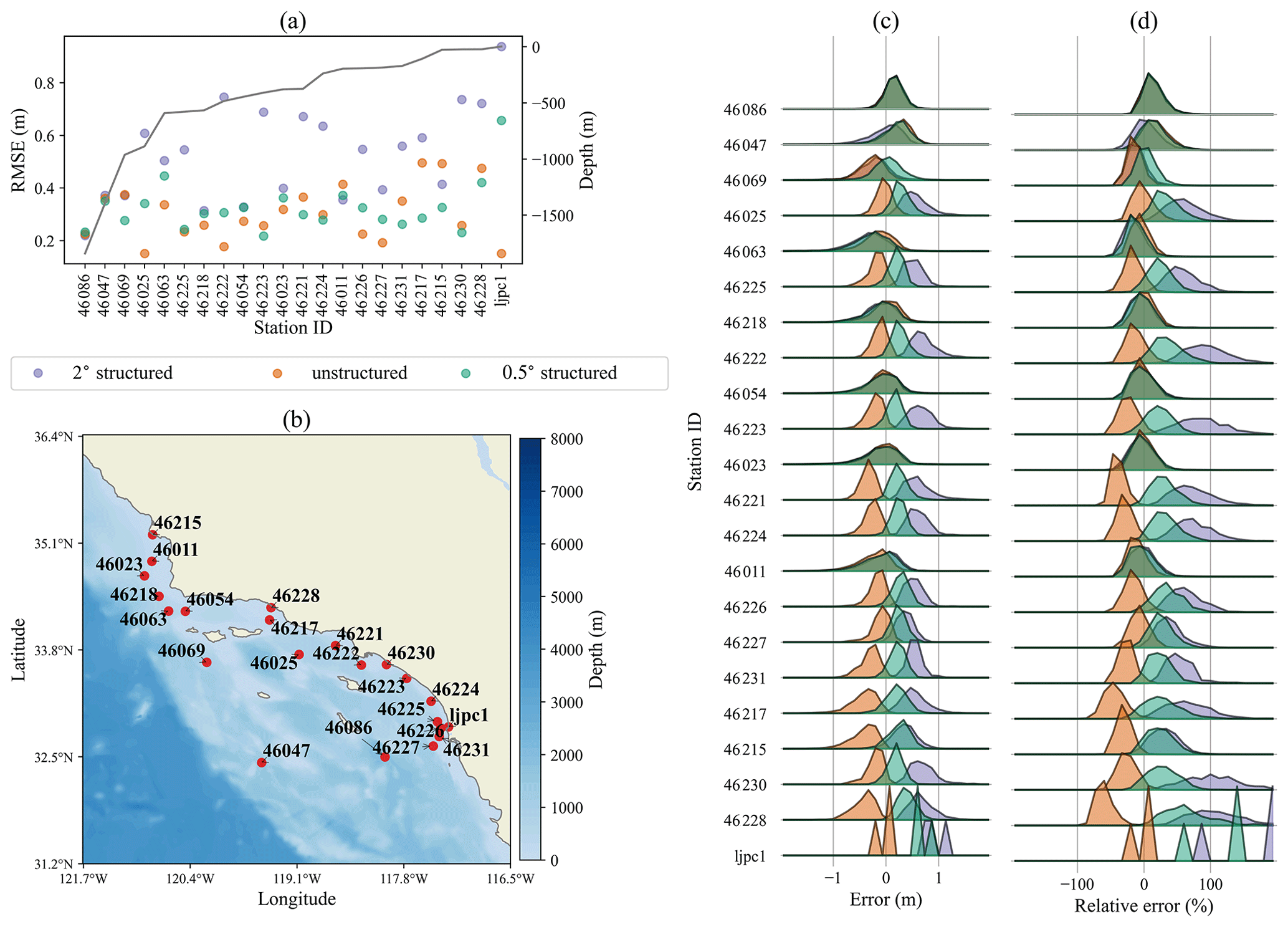
Figure 7 Same as Fig. 3 for stations along the Southern California coast.

4.1.6 Northern California and Pacific Northwest coast

Figure 8 shows the buoy validation results for the northern west coast of the US. As with the other west coast stations in Fig. 7, this coast experiences a swell-dominated wave climate. This region has a very narrow shelf, which is difficult to adequately resolve at 0.5^∘ resolution. Again, the unstructured mesh results typically underestimate both of the structured mesh solutions. All models perform similarly at the deep water stations. The unstructured mesh has some difficulties in this region; it has similar RMSE values as the 2^∘ mesh solution at stations 46213, 46014, 46229, 46013, 46050, 46212, and 46211. This could possibly be mitigated by providing additional resolution along the coastline to better resolve the narrow shelf in this region. The tails of the error distributions for the unstructured mesh tend to be eliminated in the relative error distributions. Again, this indicates that the largest errors occur during the largest observed wave heights.

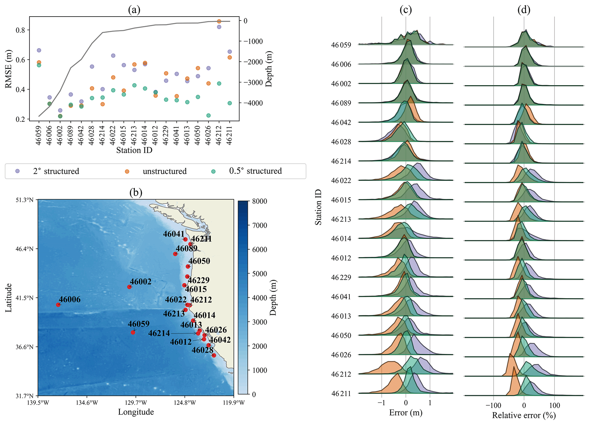
Figure 8 Same as Fig. 3 for stations along the Northern California and Pacific Northwest coast.

4.1.7 Alaskan coast

For the Alaska region shown in Fig. 9, the models again perform similarly at the deep stations with the unstructured and 0.5^∘ meshes having a slight accuracy advantage. The unstructured mesh shows a large improvement over the 2^∘ mesh at station 46060, but it is the least accurate solution at the nearby station 46061. Other than these two stations, the unstructured mesh agrees well with the 0.5^∘ structured grid.

Figure 9 Same as Fig. 3 for stations in the Alaskan coastal region.

4.1.8 Hawaiian coast

The final station region considered is around the Hawaiian Islands as shown in Fig. 10. The deep water stations again show equivalent accuracy for all three mesh resolutions. Near the island of O'ahu, the unstructured mesh is the most accurate solution at station 51201 and the least accurate at 51202. The island of Hawaii is the only Hawaiian island that is explicitly resolved in the mesh, so the results at these two stations are heavily dependent on the unresolved source term parameterization.

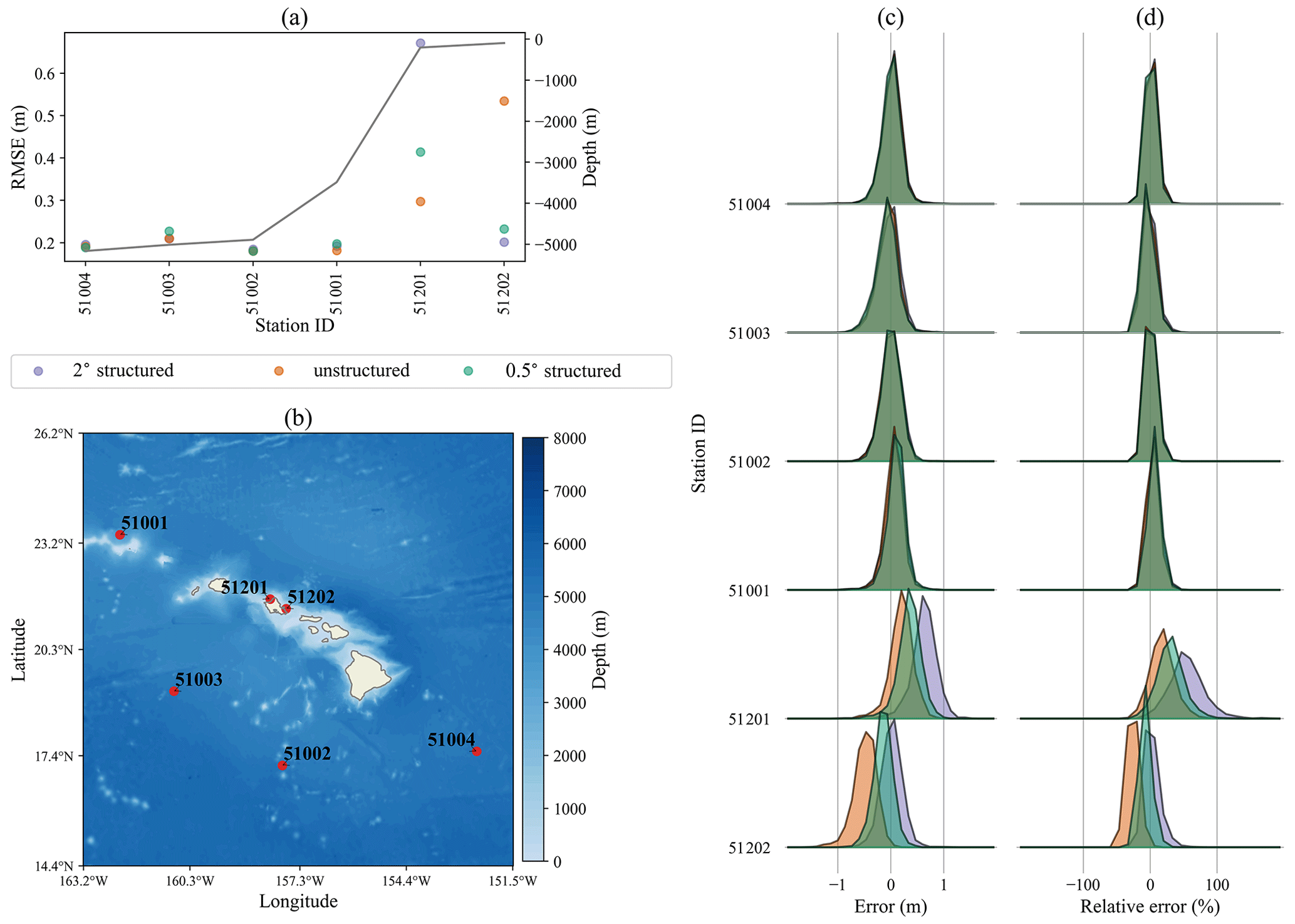
Figure 10 Same as Fig. 3 for stations near the Hawaiian islands.

4.2 Global solution differences

The results from the previous section show that, overall, the 0.5^∘ structured mesh provides the most accurate significant wave height results – although the unstructured results are often comparable, as illustrated at many stations. Taking the 0.5^∘ structured results as the “reference” solution, we now show global averaged and maximum solution differences against the 0.5^∘ structured mesh plotted for the 2^∘ structured and unstructured solutions. Of course, this comparison neglects inherent biases of the modeled results with respect to observations. However, it demonstrates spatially that the deep ocean accuracy is largely unaffected by increased resolution, while in the refined coastal regions, the unstructured mesh is in better agreement with the 0.5^∘ structured mesh.

Figure 11 shows that in the deep ocean, the unstructured and 2^∘ meshes have similar differences compared to the 0.5^∘ mesh. Especially in the equatorial regions, the solutions for these grids compare well to the 0.5^∘ solution in terms of both mean and maximum differences. The unstructured mesh has larger mean and maximum differences in the Southern Ocean, especially south of Africa. Figure 12 shows the average and maximum relative differences for the 2^∘ structured and unstructured meshes compared to the 0.5^∘ structured mesh. The large discrepancies in the Southern Ocean found in Fig. 11 are not as apparent on a relative basis because large waves are present in that area year round. The mean absolute relative difference between the 0.5^∘ structured mesh for both the 2^∘ structured and unstructured meshes is around 5 % over most of the deep ocean basins.

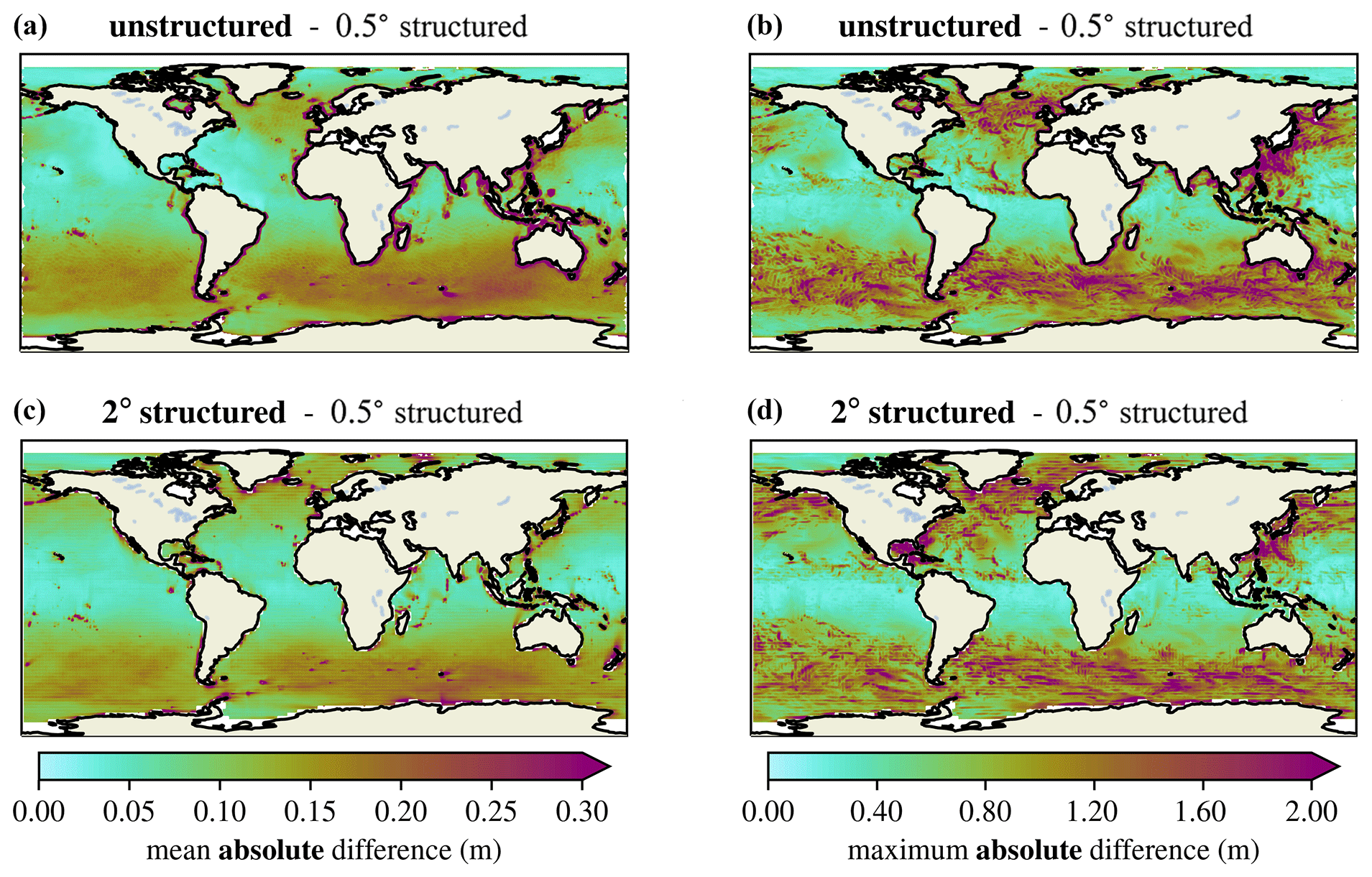
Figure 11 Mean (a, c) and maximum (b, d) absolute differences in significant wave height between the unstructured and 0.5^∘ structured meshes (a, b) and the 2 and 0.5^∘ structured meshes (c, d).

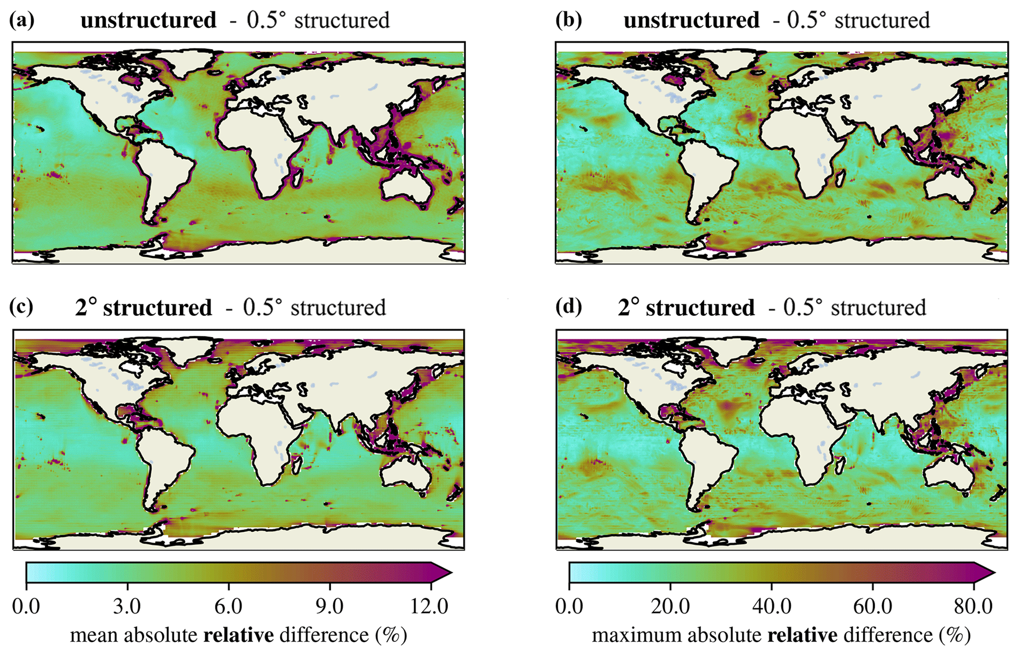
Figure 12 Mean (a, c) and maximum (b, d) absolute relative differences in significant wave height between the unstructured and 0.5^∘ structured meshes (a, b) and the 2 and 0.5^∘ structured meshes (c, d). Note this is different from Fig. 11, which shows absolute differences.

In the refined coastal areas of the unstructured mesh, the solution provides a much better agreement with the 0.5^∘ structured mesh in terms of both mean and maximum differences. Generally, improvements for the mean are better expressed by the absolute differences in Fig. 11, while the improvement in the maximum differences can be seen more clearly on a relative basis, as shown in Fig. 12.

In particular, the Gulf of Mexico benefits the most from the regional refinement of the unstructured mesh. In this area, average relative differences of around 10 % are reduced to around 3 % in the unstructured mesh. Again, the 0.5^∘ structured mesh and unstructured mesh have the same resolution throughout this area, so good agreement is expected for the wind-sea-dominated conditions. The US east coast also benefits from the unstructured refinement, especially in terms of absolute maximum differences. The same is true for the maximum absolute differences in the Gulf of Alaska.

Note that differences from individual high wind events appear to be “imprinted” in the difference plots. This is due to the relatively short June–October time period used in this study. A longer simulation period would produce a more even distribution of maximum differences. Another factor that contributes to these large maximum differences is the low resolution of the wind forcing for the 2^∘ structured mesh and in the coarse regions of the unstructured mesh. The 2^∘ resolution cannot accurately capture storm systems, leading to a more diffuse wind field. Therefore, larger differences in maximum significant wave height are associated with the lower-fidelity representation of intense wind events.

There are also greater coastal differences in the 2^∘ portions of the unstructured mesh as compared to the 2^∘ structured mesh. This is because the unstructured mesh better conforms to the coastlines at this resolution, which gives it more overlap with the 0.5^∘ structured mesh in these regions. However, due to the coarse 2^∘ resolution, the accuracy in these shallow coastal areas suffers in the unstructured mesh. The combination of these factors leads to bands of high error that are not present in the 2^∘ structured mesh because of reduced overlap with the 0.5^∘ structured mesh in coastal regions.

4.3 Performance and scalability

A strong scaling study was performed to assess the efficiency gains of the unstructured mesh. For each of the three meshes, a series of 1-month runs was performed using between 36 and 1800 processors. All point, field, and restart file output was turned off to directly compare the time required to compute the solution. Each timing is based on an average of three runs. The timing simulations were performed on the Grizzly cluster, which is a part of Los Alamos National Laboratory's Institutional Computing Program. Each Grizzly node has 128 GB of memory and is composed of two 18-core E5 2695v4 Broadwell processors, each with a clock speed of 2.1 GHz. The network is built on the Intel Omni-Path Architecture with 100 Gbps bandwidth.

The parallelization strategy for structured WW3 meshes is based on a “card-deck” approach (Tolman, 2002). In this approach, the cells are distributed to processors in a round-robin fashion. The source term calculation and intra-spectral propagation are computed in parallel, and the data are gathered onto a single core to perform the propagation in geographic space. This method incurs more data communication than a traditional domain decomposition approach. However, it has been shown to scale and has the advantage that the same parallel scheme can be used regardless of the spatial propagation method.

A traditional domain decomposition method has also been developed for the unstructured grids. In our comparison, we have chosen to use the card-deck approach to fairly compare across the structured and unstructured mesh configurations because domain decomposition is not available for the structured meshes in the existing WW3 source code. A comparison of the card-deck and domain decomposition approaches can be found in Abdolali et al. (2020).

Figure 13 shows the scaling results for each of the three mesh resolutions. The 0.5^∘ structured mesh scales nearly ideally until 576 cores and begins to experience a slowdown after 1152 cores. The unstructured mesh begins to scale less than ideally after 72 cores because of the reduced size of the mesh but continues to experience a speedup until 576 cores. Because it has the smallest number of cells, the 2^∘ mesh does not scale after 72 cores. Even with its improved scaling, the 0.5^∘ mesh does not achieve faster runtimes than the unstructured mesh. It is 2.2 times slower than the unstructured mesh at 1152 cores, which is the point at which both meshes stop experiencing a speedup with increasing core count. Due to the scaling advantage of the unstructured mesh over the 2^∘ mesh, the runtimes between the two meshes become nearly equal at 1152 cores. The throughput in terms of simulated years per day peaks at 12.1, 10.9, and 4.9 for the 2^∘, unstructured, and 0.5^∘ meshes, respectively.

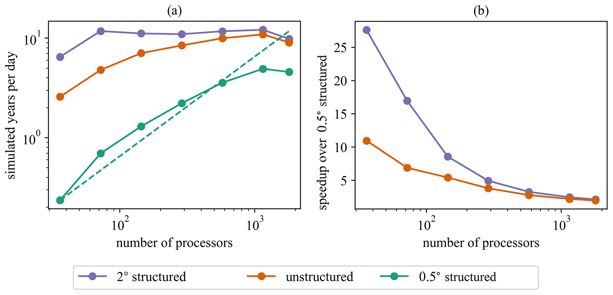
Figure 13 (a) Throughput in terms of simulated years per day based off a 1-month simulation with each mesh. The dashed line represents ideal scaling for the 0.5^∘ structured grid. (b) Speedup for the unstructured and 2^∘ meshes over the 0.5^∘ structured grid for each core count.

5 Discussion

In general, our results show that unstructured meshes can be used globally to match the accuracy of high-resolution uniform structured meshes in regions of interest at reduced cost. Figure 12 demonstrates that mean relative differences between 2 and 0.5^∘ resolution in the deep ocean are generally less than 5 %. This means the benefit to having increased resolution in these regions is minimal. However, Table 3 shows that the 0.5^∘ coastal resolution of the unstructured mesh provides substantial accuracy improvements over the 2^∘ structured mesh in shallow regions. In some cases, the unstructured mesh reduces the average relative errors in coastal regions by half, as compared to the 2^∘ mesh. This puts the coastal accuracy of the unstructured mesh near that of the 0.5^∘ mesh but for lower computational cost. In terms of computational efficiency, the unstructured mesh is 2–10 times faster than the 0.5^∘ structured mesh, depending on the number of cores used.

Another advantage of this approach is that global unstructured meshes are more flexible and are simpler to configure than two-way nested structured grids. The emergence of flexible and robust open-source mesh generation tools such as OceanMesh2D (Roberts et al., 2019) and JIGSAW(GEO) (Engwirda, 2017) has reduced the difficulty that was previously associated with generating unstructured meshes. These tools allow for arbitrary resolution specification and produce high-quality meshes that can be used directly in simulation.

There are, however, some challenges associated with unstructured meshes in practice. One of these issues is the representation of the coastlines with increasing resolution in coastal regions. Figure 14 shows the coastline differences between the unstructured and 0.5^∘ meshes. As the coastline resolution in the unstructured mesh begins to resolve details of the coast, the resulting coastline geometry can lead to local inaccuracies. For example, single-element islands can be more accurately described using the unresolved obstacle terms than by being explicitly represented in the mesh. Another example is near the Mississippi River Delta in the Gulf of Mexico. Here, the delta is just beginning to be resolved, which leads to an exaggerated sheltering effect that is not present in the structured mesh. The mesh could be altered to mitigate these issues but this was not explored here for consistency and to avoid accidental “mesh tuning” of the results.

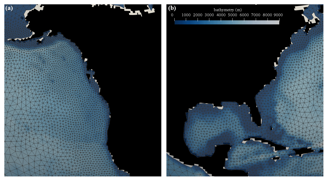
Figure 14 Differences in coastline representation between the 0.5^∘ structured and unstructured meshes for the US west coast (a) and US east coast/Gulf of Mexico (b). The structured mesh coastline is represented in black. The white regions and overlap between the black coastline and the triangular elements indicate mismatches in the mesh boundaries.

Subgrid modeling of islands and other unresolved obstacles is a critical source term needed to achieve good results with the unstructured mesh. Figure 15 shows the large errors that are obtained by excluding this source term for both the open ocean and coastal regions. The major advantage of the source term approach is that it can be applied to the unstructured mesh, unlike the discretization-level approach that is implemented for structured grids in WW3.

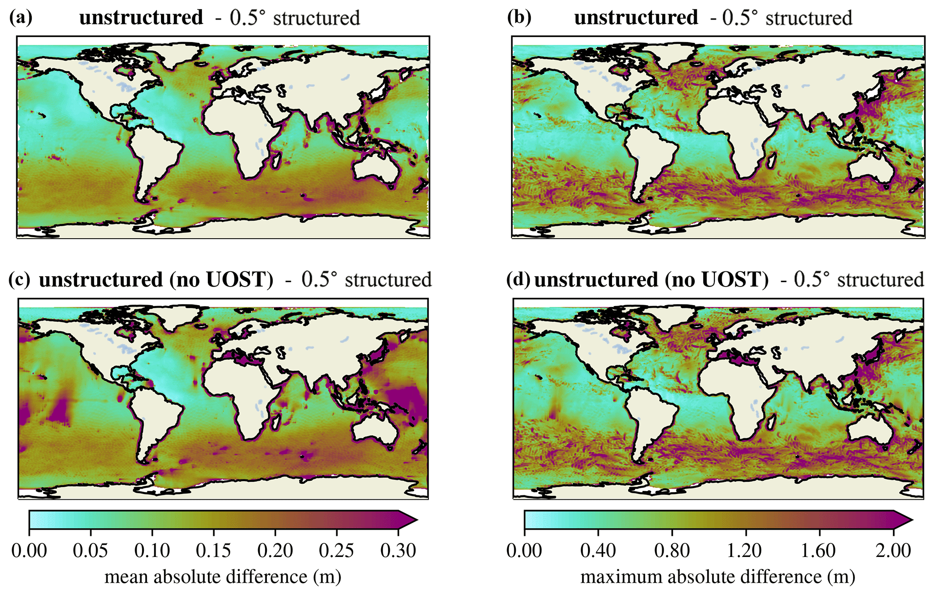
Figure 15 Mean (a, c) and maximum (b, d) absolute differences in significant wave height between the unstructured mesh with the UOST and 0.5^∘ structured grid (a, b) and between the unstructured mesh without the UOST and 0.5^∘ structured mesh (c, d).

Additional performance gains are expected to be possible using the unstructured mesh via implicit time-stepping methods, which are not as useful for structured meshes. The implicit method is advantageous for meshes that vary drastically in resolution since the smallest element size no longer dictates the maximum stable time step. A comparison between the explicit and implicit approaches can be found in Abdolali et al. (2020).

The unstructured mesh presented here is based on a simple, depth-based refinement criterion that transitions between 2 and 0.5^∘ resolutions. A generic mesh was used to make a clean comparison between structured meshes with those two grid spacings, not to optimize for accuracy. This approach details the potential of unstructured meshes to provide accuracy across the global and coastal scales, even for general meshing approaches. However, unstructured meshes also provide flexibility to consider other mesh design criteria or provide more focused resolution in specific regions. The results presented here could be improved in particular regions via targeted mesh design criteria.

As noted, the unstructured mesh results tend to consistently underpredict observations in swell-dominated regions. This is likely due to the different numerical scheme which may be more diffusive. Since the bias is consistent, tuning the β_max value as was done in Rascle and Ardhuin (2013) may be a viable way to reduce this bias. However, in this study, we have chosen to keep all the parameters consistent across the mesh configurations.

Overall, when compared with the 0.5^∘ structured mesh, the unstructured mesh seems to perform very well in coastal wind-sea-dominated environments, such as the Gulf of Mexico and US east coast. Swell-dominated environments, such as the US west coast and Alaska, tend to have larger errors for the unstructured case but still represent an overall improvement in accuracy compared to the 2^∘ structured mesh. Ultimately, unstructured meshes can accommodate global to coastal resolution across various coastal environments without sacrificing accuracy or efficiency.

6 Conclusions

Our results demonstrate the accuracy and efficiency advantages of global unstructured meshes compared to a single structured grid. By varying resolution across deep and shallow regions, unstructured meshes are able to match the efficiency of coarser-resolution structured meshes in the global ocean without sacrificing accuracy in high-resolution coastal areas. This capability has the potential to greatly reduce the computational cost of including waves into Earth system models.

The validations presented show that in coastal regions, the unstructured mesh considered here was as accurate as the 0.5^∘ structured mesh. The unstructured mesh provided a factor of 2–10 speedup over the global 0.5^∘ structured mesh depending on the number of cores used. This increase in performance comes with substantial coastal accuracy gains over the global structured 2^∘ results.

The unstructured WW3 capability combined with the variable-resolution philosophy of E3SM is a viable approach to including waves in coupled Earth system simulations. This allows interfacial interactions between the atmosphere and ocean to be directly simulated via inclusion of wave physics in WW3. The performance of this approach is expected to allow for consideration of an expanded range of science applications including coastal flooding, coastal biogeochemistry, and wave–sea ice interactions at high latitudes. Inclusion of wind-wave processes, especially for coastal simulations, is needed for next-generation Earth system models as resolution and overall complexity increase. These interactions between coupled components will begin to require resolution of subgrid processes dependent upon wave conditions as directly simulated by WW3. The advantages of unstructured WW3 make it ideal for use in next-generation, variable-resolution Earth system models like E3SM.

Appendix A: Differences between first- and third-order schemes for structured meshes

As mentioned in Sect. 3.4, typical WW3 structured mesh configurations use the third-order ULTIMATE QUICKEST scheme instead of the first-order method used here for comparison with the first-order unstructured CRD-N scheme. Figure A1 shows the accuracy differences between the PR1 and PR3 $/$ UQ switches for the 0.5^∘ and 2^∘ structured meshes. Each subplot represents validation results from buoys in the regions from Sects. 3–10. These plots demonstrate that while the PR3 $/$ UQ scheme is slightly more accurate overall, the choice of numerical scheme for the structured meshes does not change the conclusions of our study.

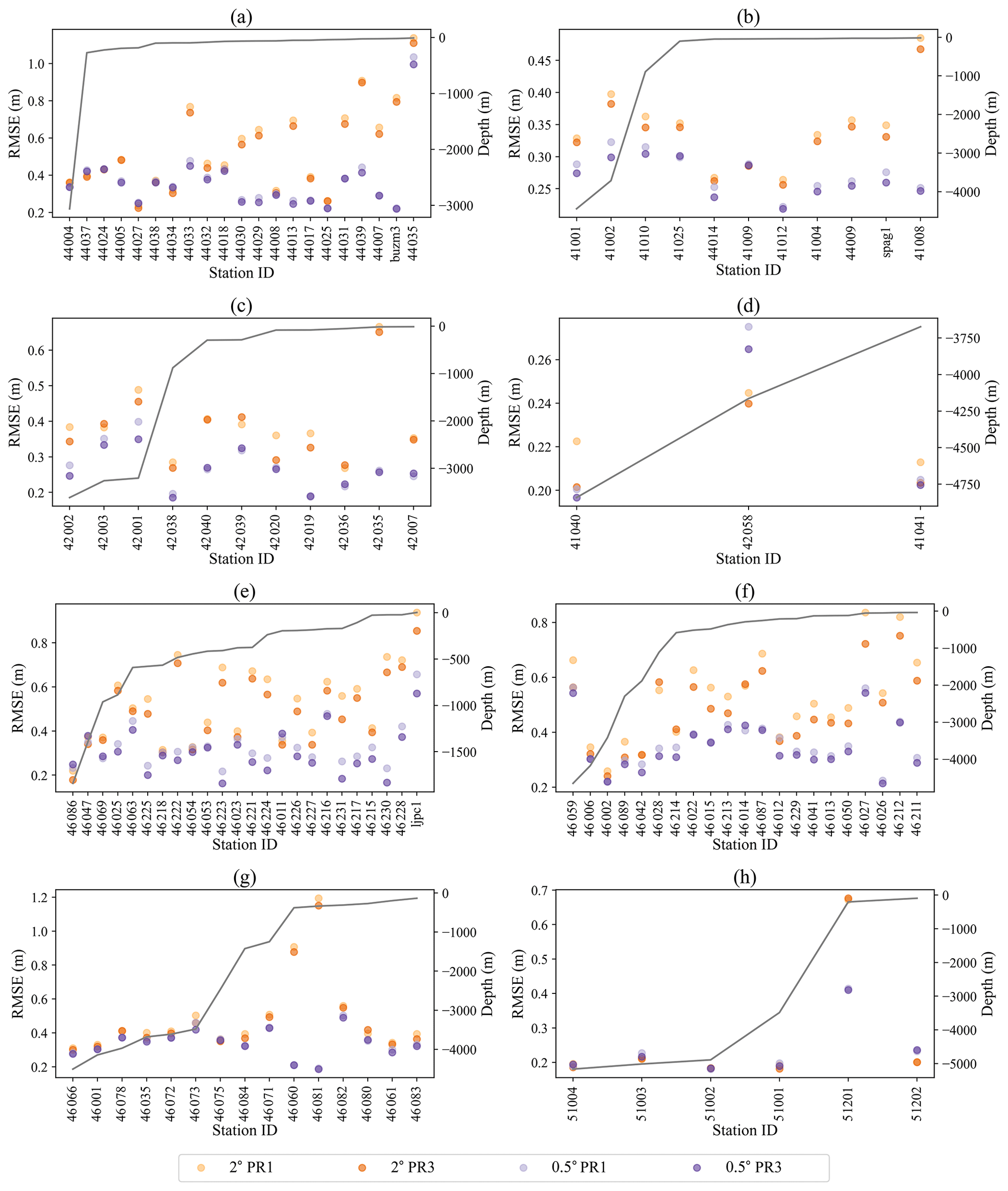
Figure A1 Root mean square errors comparing the accuracy differences between the PR1 and PR3 + UQ switches. The 2^∘ structured mesh is represented by orange and the 0.5^∘ structured mesh is shown in purple. Darker shades are associated with the PR3 configuration, while lighter shades correspond to the PR1 switch. Subplots are presented in order of regions from the paper as follows: (a) Gulf of Maine, (b) southern to mid-Atlantic east coast, (c) Gulf of Mexico, (d) Caribbean region, (e) Southern California coast, (f) Northern California and Pacific Northwest coast, (g) Alaskan coast, and (h) Hawaiian coast.