the Creative Commons Attribution 4.0 License.
the Creative Commons Attribution 4.0 License.
 | 20 May 2021
The Community Multiscale Air Quality (CMAQ) model versions 5.3 and 5.3.1: system updates and evaluation
K. Wyat Appel
Jesse O. Bash
Kathleen M. Fahey
Kristen M. Foley
Robert C. Gilliam
Christian Hogrefe
William T. Hutzell
Daiwen Kang
Rohit Mathur
Benjamin N. Murphy
Sergey L. Napelenok
Christopher G. Nolte
Jonathan E. Pleim
George A. Pouliot
Havala O. T. Pye
Limei Ran
Shawn J. Roselle
Golam Sarwar
Donna B. Schwede
Fahim I. Sidi
Tanya L. Spero
David C. Wong
The Community Multiscale Air Quality (CMAQ) model version 5.3 (CMAQ53), released to the public in August 2019 and followed by version 5.3.1 (CMAQ531) in December 2019, contains numerous science updates, enhanced functionality, and improved computation efficiency relative to the previous version of the model, 5.2.1 (CMAQ521). Major science advances in the new model include a new aerosol module (AERO7) with significant updates to secondary organic aerosol (SOA) chemistry, updated chlorine chemistry, updated detailed bromine and iodine chemistry, updated simple halogen chemistry, the addition of dimethyl sulfide (DMS) chemistry in the CB6r3 chemical mechanism, updated M3Dry bidirectional deposition model, and the new Surface Tiled Aerosol and Gaseous Exchange (STAGE) bidirectional deposition model. In addition, support for the Weather Research and Forecasting (WRF) model's hybrid vertical coordinate (HVC) was added to CMAQ53 and the Meteorology-Chemistry Interface Processor (MCIP) version 5.0 (MCIP50). Enhanced functionality in CMAQ53 includes the new Detailed Emissions Scaling, Isolation and Diagnostic (DESID) system for scaling incoming emissions to CMAQ and reading multiple gridded input emission files.
Evaluation of CMAQ531 was performed by comparing monthly and seasonal mean daily 8 h average (MDA8) O3 and daily PM2.5 values from several CMAQ531 simulations to a similarly configured CMAQ521 simulation encompassing 2016. For MDA8 O3, CMAQ531 has higher O3 in the winter versus CMAQ521, due primarily to reduced dry deposition to snow, which strongly reduces wintertime O3 bias (2–4 ppbv monthly average). MDA8 O3 is lower with CMAQ531 throughout the rest of the year, particularly in spring, due in part to reduced O3 from the lateral boundary conditions (BCs), which generally increases MDA8 O3 bias in spring and fall (∼0.5 µg m−3). For daily 24 h average PM2.5, CMAQ531 has lower concentrations on average in spring and fall, higher concentrations in summer, and similar concentrations in winter to CMAQ521, which slightly increases bias in spring and fall and reduces bias in summer. Comparisons were also performed to isolate updates to several specific aspects of the modeling system, namely the lateral BCs, meteorology model version, and the deposition model used. Transitioning from a hemispheric CMAQ (HCMAQ) version 5.2.1 simulation to a HCMAQ version 5.3 simulation to provide lateral BCs contributes to higher O3 mixing ratios in the regional CMAQ simulation in higher latitudes during winter (due to the decreased O3 dry deposition to snow in CMAQ53) and lower O3 mixing ratios in middle and lower latitudes year-round (due to reduced O3 over the ocean with CMAQ53). Transitioning from WRF version 3.8 to WRF version 4.1.1 with the HVC resulted in consistently higher (1.0–1.5 ppbv) MDA8 O3 mixing ratios and higher PM2.5 concentrations (0.1–0.25 µg m−3) throughout the year. Finally, comparisons of the M3Dry and STAGE deposition models showed that MDA8 O3 is generally higher with M3Dry outside of summer, while PM2.5 is consistently higher with STAGE due to differences in the assumptions of particle deposition velocities to non-vegetated surfaces and land use with short vegetation (e.g., grasslands) between the two models. For ambient NH3, STAGE has slightly higher concentrations and smaller bias in the winter, spring, and fall, while M3Dry has higher concentrations and smaller bias but larger error and lower correlation in the summer.
- Article
(31156 KB) - Full-text XML
-
Supplement
(36376 KB) - BibTeX
- EndNote


To help protect human health and the environment, many countries and government organizations around the world have set limits for atmospheric pollutants. Established in 1970 and working under the direction of the Clean Air Act (CAA) of 1970 and revised CAA of 1990 (https://www.epa.gov/clean-air-act-overview, last access: 3 May 2021), the United States Environmental Protection Agency (USEPA) is mandated to periodically review and propose revised limits or national ambient air quality standards (NAAQS; Bachmann, 2007) for criteria air pollutants in the US, including ground-level ozone (O3) and PM2.5 (particulate matter with an effective aerodynamic diameter less than 2.5 µm). The current US NAAQS for ground-level O3 is 0.070 parts per million by volume (ppmv) and is based on the maximum of a rolling 8 h average throughout the day (MDA8 O3). The current US NAAQS for PM2.5 is 35 µg m−3 for a daily average and 12 µg m−3 for an annual average. Areas above the NAAQS are in “nonattainment” and are required to implement measures that reduce observed O3 and/or PM2.5 to be below the NAAQS within a specified period. These measures typically require reducing anthropogenic emissions within the area of nonattainment, as both O3 and PM2.5 are principally formed in the atmosphere through a complex series of chemical reactions from primary emitted pollutants. For O3, these precursor pollutants are oxides of nitrogen (NO and NO2) and volatile organic compounds (VOCs) such as isoprene and formaldehyde (HCHO), which undergo photochemical reactions in the atmosphere to form ground-level O3. In contrast, ambient PM2.5 arises from both primary emissions and complex chemical reactions, leading to formation of its diverse inorganic and organic chemical constituents. Therefore, a much larger system of emission sources and atmospheric reactions must be considered for PM2.5 formation. In addition to the formation of these pollutants, there are numerous processes that also destroy (e.g., titration, photolysis, oxidation) and remove (e.g., dry deposition, wet scavenging) these pollutants from the atmosphere.
Given the complexity of O3 and PM2.5 formation, transport, destruction, and deposition, the groups responsible for developing plans to reduce these pollutants (e.g., state governments, multi-jurisdictional organizations) generally rely on numerical models to simulate the processes involved and estimate the outcomes of plausible control strategies. The Community Multiscale Air Quality (CMAQ) model (Byun and Schere, 2006), developed and distributed by the USEPA is a state-of-the-science numerical air quality model with comprehensive representations of the emission, transport, formation, destruction, and deposition of many air pollutants, including O3 and PM2.5. The first version of CMAQ was released more than 20 years ago and has been continually updated to incorporate the latest available scientific information and improve overall model performance. CMAQ version 5.3 (CMAQ53; United States Environmental Protection Agency, 2019a) was released in August 2019 and was followed by a minor update in December 2019 to version 5.3.1 (CMAQ531, United States Environmental Protection Agency, 2019b). Prior to these two versions, the previous version of CMAQ was version 5.2.1 (CMAQ521; United States Environmental Protection Agency, 2018) released in July 2018. The most recently published comprehensive review and evaluation of CMAQ was conducted for version 5.1 (Appel et al., 2017), although numerous articles on specific scientific updates to CMAQ have been published since then.
Here we describe the scientific updates in CMAQ53, review several of the updates that improve simulation speed and enhance capabilities, and present a comparison against the previous release (i.e., CMAQ521). Some of the major scientific enhancements in CMAQ53 include updates to aerosol formation, including monoterpene secondary organic aerosol (SOA) formation and uptake of water onto hydrophilic organic aerosol (OA), updates to the M3Dry deposition and bidirectional ammonia (NH3) exchange model, the new Surface Tiled Aerosol and Gaseous Exchange (STAGE) deposition model, and updates to marine halogen and chlorine chemistry. Examples of enhanced capabilities in CMAQ53 include the new Detailed Emissions Scaling, Isolation, and Diagnostic (DESID) module, which provides the ability to scale emissions directly through a single control file, the updated Integrated Source Apportionment Method (ISAM; Kwok et al., 2013, 2015) for source tracking and attribution, and the updated Sulfur Tracking Method (STM). The operational evaluation of the new modeling system uses 2016 annual simulations that cover the conterminous United States and large portions of Canada and northern Mexico. This evaluation quantifies the impacts of the scientific updates in CMAQ53 on model performance as compared to CMAQ521, while also analyzing the impacts other system updates (i.e., meteorology, boundary conditions, and deposition model) on model performance.
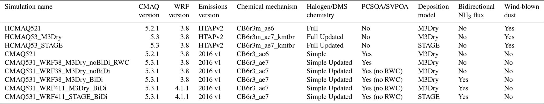
Scientific updates in CMAQ are contributed by many different researchers, who may work for years to develop and test that update. This section primarily focuses on only the most impactful scientific updates in CMAQ53, determined by examining the impacts of each change on concentrations of O3 and PM2.5. As such, this section does not exhaustively review the science updates made in CMAQ53. Additional details on the updates presented here, along with information regarding all other updates to CMAQ53 and CMAQ531, are in the release notes and documentation on the CMAQ GitHub web page (https://github.com/USEPA/CMAQ, last access: 3 May 2021). While many of the major updates to the CMAQ53 modeling system are discussed in Sect. 2, only a subset of those updates is evaluated and presented in Sect. 4; see Table 1 for a list of the model simulations and their configurations.
Table 1Names and configurations of the hemispheric and regional CMAQ simulations.
2.1 Chemistry
There are three basic families of chemical mechanisms implemented in CMAQ: Carbon-Bond (CB), Statewide Air Pollution Research Center (SAPRC), and the Regional Atmospheric Chemical Mechanism (RACM). Of the three families of mechanisms available, CB tends to be the most widely used for regional air quality applications with CMAQ, and CB6r3 is the most recent version of CB implemented in CMAQ53. While the CB6r3 name is retained in CMAQ53, the version of CB6r3 in CMAQ53 differs from the original version implemented outside of CMAQ. This section describes updates made in the CB6r3 chemical mechanism and associated aerosol chemistry in CMAQ53.
2.1.1 Updates to the chlorine chemistry
The chlorine chemistry in the CB6r3 chemical mechanism (Yarwood et al., 2014; Luecken et al., 2019) has been updated in CMAQ53. A new model species, chlorine nitrate (ClNO3), and several new reactions (including heterogeneous hydrolysis of ClNO3) have been added. The chlorine chemistry in CMAQ52 contained 26 chemical reactions and 7 chlorine species, while the chlorine chemistry in CMAQ53 contains 31 chemical reactions and 8 chlorine species. All versions of the CB6 chemical mechanism in CMAQ53 use the same chlorine chemistry. An updated Euler backward iterative (EBI) solver was also developed for the revised mechanisms. Model sensitivity simulations show that including the ClNO3 chemistry decreases monthly mean O3 by 0.1–0.5 parts per billion by volume (ppbv). The impact of the updated chlorine chemistry on aerosols is small.
2.1.2 Addition of the bromine and iodine chemistry
Detailed bromine and iodine (halogen) chemistry (Sarwar et al., 2015) was included in a prior version of the CB mechanism (i.e., CB05) in CMAQ52. Sarwar et al. (2019) updated the detailed bromine and iodine chemistry in CB05 in CMAQ521 and examined its impact on O3 using the hemispheric CMAQ (HCMAQ) model. The bromine and iodine chemistry was further adapted for the CB6r3 chemical mechanism and implemented into CMAQ53. The updated chemistry contains 38 gas-phase reactions, 4 heterogeneous reactions and 5 aqueous-phase reactions for bromine species, and 44 gas-phase reactions and 10 heterogeneous reactions for iodine species. The detailed bromine and iodine chemistry is more active in the HCMAQ model, where marine environments represent large extents of the modeled domain in which halogen chemistry influences air masses as they traverse vast extents of oceans during intercontinental transport. However, this update can also be used in the regional version of the model. Based on HCMAQ model sensitivity simulations for October–December 2015, the detailed bromine and iodine chemistry in CB6r3 reduces O3 by an average of 3.0–14 ppbv over much of the open-ocean area for the 3-month period. Its impact over coastal regions is greater than over the interior portion of land, where changes are smaller but non-negligible. The details of the updated bromine and iodine chemistry in CMAQ and its impact on O3 are described in Sarwar et al. (2019).
2.1.3 Addition of the DMS chemistry
Dimethyl sulfide (DMS) chemistry has been combined with CB6r3 and implemented into CMAQ53. The DMS chemistry in CMAQ contains seven gas-phase reactions involving DMS and oxidants (OH, NO3, Cl, ClO, IO, BrO). The reactions of DMS with oxidants produce sulfur dioxide (SO2), which can further be converted into sulfate (SO) through both gas- and aqueous-phase SO2 oxidation pathways already in CMAQ (Sarwar et al., 2011). The combined chemical mechanism containing CB6r3, detailed bromine and iodine, and DMS chemistry is named CB6r3m. Based on HCMAQ model sensitivity simulations for October–December 2015, introducing DMS chemistry into CB6r3 increases SO2 by an average of 20–160 pptv and SO by 0.1–0.8 µg m−3 over much of the open-ocean area for the 3-month period. Changes over land are smaller and primarily limited to coastal regions. The details of the DMS chemistry in CMAQ and its impact are described in Zhao et al. (2021).
2.1.4 Updates to the simple halogen-mediated O3 loss
Computational efficiency is important for chemical transport models (CTMs) because their use in air quality management requires exploring various emission scenarios. The detailed bromine and iodine (halogen) chemistry increases the computational demand of the model; thus, a simplified first-order rate constant was previously developed for calculating halogen-mediated O3 loss over seawater (which is applied through all vertical layers) (Sarwar et al., 2015) for use in regional CMAQ model applications with limited seawater in the domain and incorporated into a previous version of CMAQ. This rate constant has been updated in CB6r3 and incorporated into CMAQ53. The newly calculated first-order surface O3 loss rate is approximately 10 % greater than that used in CMAQ521. Model sensitivity simulations over the conterminous US domain with the existing and updated simple first-order O3 loss rate suggests that the updated simple first-order halogen-mediated O3 loss further reduces monthly average O3 by up to 4.0 ppbv over seawater and up to 2.0 ppbv in coastal areas. This simple halogen-mediated O3 loss is used in all chemical mechanisms in CMAQ except in the detailed bromine and iodine chemistry.
2.1.5 AERO7/7i
The aerosol chemistry in CMAQ53 has been significantly updated and is available as a new aerosol module called AERO7. The aerosol model from CMAQ521, AERO6, is still available for use with CMAQ53. The version of the aerosol module used by CMAQ is a build-time option that is tailored for the chosen chemical mechanism (e.g., cb6r3_aero6 and cb6r3_aero7), with only that specific aerosol version then available for that specific executable.
The AERO7 module in CMAQ53 improves consistency in representing SOA formation pathways between the CB- and SAPRC-based chemical mechanisms, updates monoterpene SOA yields from photooxidation (OH and O3), adds uptake of water onto hydrophilic organics (Pye et al., 2017), adds consumption of inorganic SO when isoprene epoxydiol (IEPOX) organosulfates are formed, and improves computational efficiency by parameterizing anthropogenic SOA yields through a volatility basis set (VBS) instead of an Odum 2-product fit (Qin et al., 2021). The 21 new species in the AERO7/7i modules are listed in Table S1. In addition, monoterpene nitrates and their SOA products (Pye et al., 2015) are new to the AERO7 module but were introduced in the AERO6i module in CMAQ521. There were also 28 species that were deprecated in AERO7/7i (see Table S1).
AERO7 and AERO7i modules contain the same major pathways to SOA, but AERO7i provides more diagnostic information in terms of IEPOX SOA identity (Pye et al., 2013, 2017), as well as some minor additional high-NOx pathways to SOA (a particle-phase isoprene dinitrate (Pye et al., 2015) and 2-methylglyceric acid). CMAQ users who require additional isoprene SOA speciation (e.g., to evaluate against measurements) may want to use the AERO7i module (only available for use with SAPRC07-based gas-phase chemistry with expanded isoprene intermediates, i.e., SAPRC07tic). While AERO7 (currently only linked with CB-based mechanisms) and AERO7i contain the same major SOA pathways, SOA abundances may differ between the two modules due to differences in the gas-phase oxidant budget driving SOA formation.
Monoterpene oxidation, which accounts for half of the organic aerosol in the southeastern US in summer, was significantly underestimated in CMAQ52 with AERO6 (Zhang et al., 2018) and has been updated in AERO7/7i. The Odum two-product monoterpene SOA (Carlton et al., 2010) in AERO6 was replaced in AERO7/7i with updated yields based on more recent experimental data by Saha and Grieshop (2016). The new yields are represented using a VBS fit and are applied to both OH and O3 oxidation of monoterpenes. The fit allows for prompt formation of low-volatility material, which is more consistent with recent observations, indicating autoxidation is a major contributor to monoterpene SOA (Pye et al., 2019). No additional chemistry, such as oligomerization, is applied to the prompt yields. The updated monoterpene photooxidation matched well with ambient observations in the southeastern US for different seasons (Xu et al., 2018). While seven VBS bins were used in the implementation of Xu et al. (2018), the highest-volatility bin was not included in the AERO7 implementation as it had very minor contributions to the SOA, even under cold conditions with high loadings.
Finally, there are some emission speciation updates required when using the AERO7 module with CB6r3 in CMAQ53, particularly when using emissions previously generated for the AERO6 module with CB chemistry in CMAQ521. AERO7/7i require that α-pinene (usually denoted APIN) is isolated from all other monoterpenes (TERP) in the model. This is to avoid making SOA from α-pinene + nitrate radical reactions, as that pathway has been shown to produce negligible SOA (Fry et al., 2014). All SAPRC07-based mechanisms, including AERO6/6i, already separate APIN from TERP, and thus SAPRC07-based AERO6/6i/7/7i emissions are compatible with any AERO module. CB6r3 with AERO6 continues to include APIN in TERP as it did in CMAQ521.
There are three options available to use CB6r3-AERO6 emissions with the CB6r3-AERO7 module. The first approach is to comprehensively and properly map monoterpene emissions by removing APIN from all other monoterpenes as part of emissions processing. The second approach is to approximate the required speciation by assuming a fraction of all emitted terpenes (e.g., 30 %, Pye et al., 2010) are APIN and use the DESID (Murphy et al., 2020) functionality to map that fraction (e.g., 30 %) of the total monoterpenes to APIN and the remaining (e.g., 70 %) to TERP. The third approach is to allow CMAQ to determine the correct biogenic mapping when using inline calculated biogenic emissions and neglect the anthropogenic monoterpene distinction between α-pinene and other monoterpenes. The third approach utilizes species to mechanism surrogate mapping profiles for biogenic VOCs in CB6r3-AERO6 and CB6r3-AERO7 available within CMAQ and is not an option when biogenic emissions that were processed offline (pre-processed) for AERO6 and are then used for AERO7.
The impact of AERO7 on model performance is presented in Sect. 4. In short, AERO7 will generally increase PM2.5 mass, primarily in summer, in vegetation-rich locations such as the southeastern US (Xu et al., 2018). Ambient PM2.5 is further increased by water uptake, which modulates aerosol optical properties and has implications for metrics such as aerosol optical depth (AOD) that represent in situ (versus dry) conditions.
2.1.6 Other aerosol processes
Several minor updates were made to the aerosol processes in CMAQ53. Specifically, the dry deposition velocities, particularly for coarse-mode particles, were too high by 10 %–100 % in CMAQ521. Detailed testing revealed that the dry deposition algorithm in CMAQ521 was not suitable for coarse-mode particles, especially when the mode width (σ) of the coarse mode approached 2.5, the upper bound. The revised algorithm in CMAQ53 reduces the strong dependence on σ and introduces a dependence on leaf area index (LAI). The LAI dependence is intended to capture the larger deposition hypothesized over, for example, forest canopies, relative to bluff-body surfaces. The net result of this algorithm update is a large reduction in coarse-mode particle deposition in some areas. However, both Aitken and coarse-mode particle deposition increase in highly vegetated areas, such as the southeastern US.
The gravitational settling algorithm in CMAQ53 was also updated because it did not conserve mass for certain aerosol size distribution parameter combinations in earlier version of CMAQ. These errors typically occurred in the highest-altitude model layers but could propagate to other parts of the domain and lower levels if the errors were large enough. CMAQ53 resolves these problems by correcting a minor error in the time step increment and by maximizing the number of iterations used to calculate settling. While these updates resolve the mass accumulation errors (up to 10 %–50 % of the total coarse mode particle mass), they minimally impact overall model performance for PM2.5 and PM10 given the infrequent and transient nature of the errors.
2.1.7 Aqueous and heterogenous chemistry
AQCHEM-KMT was introduced in CMAQ51 to provide a framework for examining detailed cloud chemistry and increase connections between cloud microphysics and chemistry by introducing a dependence of mass transfer and chemistry on droplet size (Fahey et al., 2017a). KMT refers to the category of cloud chemistry modules that are built using the Kinetic Pre-Processor (KPP) version 2.2.3 (Damian et al., 2002) and treat the mass transfer between gas and aqueous phases with the resistance model of Schwartz (1986). The use of KPP facilitates the straightforward extension of the mechanism to include treatment of additional aqueous chemical reactions beyond those considered in CMAQ's default cloud chemistry module (AQCHEM). Two additional KMT cloud chemistry options were added to CMAQ53: KMT version 2 (KMT2) (Fahey et al., 2017b; Fahey and Roselle, 2019) and KMTBR (Sarwar et al., 2019). KMTBR expands the default cloud chemistry mechanism of five S(IV) oxidation and two SOA reactions to include the treatment of aqueous chemistry for several bromine species. KMT2 builds upon CMAQ's existing in-cloud sulfur (S) oxidation chemistry, replacing the yield parameterization of in-cloud SOA formation from GLY/MGLY + OH with a mechanistic representation of small dicarboxylic acid formation from the reactions of OH with glyoxal, methylglyoxal, glycolaldehyde, and acetic acid (Lim et al., 2005, 2010, 2013; Sareen et al., 2013). It also includes additional aqueous chemistry for S, nitrogen (N), carbon (C), and hydroxide (OH−) species largely based on the aqueous mechanism of ReLACS-AQ (Leriche et al., 2013), a compact cloud chemistry mechanism built from and tested against more comprehensive models.
The species impacted and magnitude of the effects from the KMT2 update depend heavily on season and location. Simulations over the conterminous US for July 2016 showed a surface-level increase in in-cloud SOA from small carbonyl compounds (AORGC) of 400 %–600 % compared to CMAQ's standard yield-based parameterization for GLY and MGLY + OH, increasing July average organic aerosol by up to 0.5 µg m−3 in areas of the southeastern US KMT2 also shows elevated cloud SOA at the surface and aloft. A recent HCMAQ simulation using KMT2 showed monthly average changes to in-cloud SOA of up to 1.0 µg m−3 in regions and during seasons when oxidant levels and biogenic emissions were high, increasing by at least a factor of five in much of the southeastern US during the summer.
In the winter, SO is the most significantly impacted species from this update. HCMAQ simulations for January 2016 indicate a monthly average increase in SO concentrations of up to 17 % over China and 34 % over the US. Nitrate decreased with a similar pattern to the SO increase. Monthly average O3, HCHO, and NOx were minimally impacted over the conterminous US (typically within approximately 3 %), but larger absolute impacts over shorter time periods and in other regions (e.g., change in average O3 up to −11 % over Asia) were observed. Impacts of KMT2 on CMAQ runtime depend heavily on domain, season, and chemical mechanism, but it can increase runtime by 30 % or more for some CB6-based HCMAQ applications as the number of cloudy grid cells increases. KMT2 is considered a research option, and it was not used in the simulations presented here. KMTBR is used in the HCMAQ simulations here, but it was not used in the regional CMAQ simulations.
2.2 Air–surface exchange
CMAQ53 offers two air–surface exchange models: updated M3Dry and the new Surface Tiled Aerosol and Gaseous Exchange (STAGE) model. For dry deposition, both options are modified versions of the previous M3Dry model. However, NH3 bidirectional exchange (BiDi) in both options diverges from the previous M3Dry model. In both M3Dry and STAGE, the cuticular resistance of non-ionic organic species is modeled similarly to the processes involving the partitioning of semi-volatile gases to organic aerosols. Bulk leaf wax properties and composition are taken from the observations of Schreiber and Schoenherr (2009), and vapor pressure is used to estimate air cuticle partitioning following Raoult's law. Values are then used to populate a “relative reactivity” field in CMAQ, but the cuticular resistance is essentially converted from a reactivity-driven process to an absorptive partitioning process (for organic species). The following sections describe the specific updates to M3Dry in CMAQ53 and provide a brief description of the new STAGE model. More details about each model can be found in their respective publications referenced in each section.
2.2.1 Updates to the M3Dry deposition model
The new M3Dry BiDi option in CMAQ53 requires fertilization inputs that are generated by the Environmental Policy Integrated Climate (EPIC; Williams, 1995) model through the Java-based Fertilization Emission Scenario Tool for CMAQ (FEST-C; Ran et al., 2019). M3Dry in CMAQ53 has been updated to directly use the information provided by the EPIC model. M3Dry uses daily input of total ammonium (NH) from EPIC in the 1 and 5 cm soil layers, soil pH, soil moisture content, soil cation exchange capacity (CEC), and soil texture parameters for each of 42 crop types. These data are read into CMAQ53 and used to compute the amount of NH available for volatilization in the soil and the soil NH3 compensation concentration. Bidirectional NH3 flux is computed from the soil compensation concentration (the maximum of the 1 or 5 cm layer) according to the resistance model described in Pleim et al. (2013). Hourly net bidirectional NH3 flux, NH3 dry deposition, and NH3 emissions are all output in the CMAQ DRYDEP file. The capability to output land-use-specific dry deposition flux has been removed from M3Dry in CMAQ53 but can be estimated offline using available post-processing tools to accommodate ecosystem applications.
The new NH3 bidirectional flux model in M3Dry substantially changes NH3 concentrations and surface fluxes that depend on EPIC input data. The model is identical to the box model developed and evaluated against field flux measurements in Pleim et al. (2013). Details of the implementation in CMAQ53 and evaluation compared to ground sites and satellite retrievals are presented by Pleim et al. (2019). Unlike previous versions of M3Dry, the new scheme relies on direct coupling to EPIC, which includes comprehensive C-N-P cycles and daily agricultural management, to better model the soil biogeochemistry related to the soil NH4 and its availability to volatilize. Additional information about the impact on model performance of the updates to the M3Dry scheme in CMAQ53 is provided in Sect. 4 on model evaluation.
Several other important updates in M3Dry related to air–surface exchange depend on land use and areas with snow cover. First, the dry deposition to snow was updated in M3Dry to increase the O3 dry deposition resistance to snow. Specifically, the resistance was increased from 1000 to 10 000 s m−1 based on observations from Helmig et al. (2007), and thus the deposition velocity (Vd) of O3 to snow is on the order of 0.01 cm s−1. The result is a significant increase in ambient O3 mixing ratios over snow-covered areas in CMAQ53 with M3Dry. The ground resistance (Rg) for O3 has been changed to be sensitive to soil moisture (Wg) following Mészáros et al. (2009) and Fares et al. (2012):
Wfc is the soil moisture content at field capacity and Rg(O3) is limited to 500 s m−1 when Wg≥Wfc. The result is a decrease in the Rg(O3) for soil compared to CMAQ521 where Rg(O3)=667 s m−1, which decreases ambient O3 mixing ratios, as more O3 is dry deposited to the soil.
2.2.2 Surface Tiled Aerosol and Gaseous Exchange (STAGE) deposition model
STAGE is a new deposition model available in CMAQ53. The STAGE deposition model estimates fluxes from sub-grid cell fractional land-use values, aggregates the fluxes to the model grid cell, and unifies the bidirectional and unidirectional deposition schemes using the resistance model frameworks of Massad et al. (2010) and Nemitz et al. (2001). Modeled parameterizations are the same land-use-specific versions employed in M3Dry expect for those parameterizations detailed in this section and the quasi-laminar boundary layer resistances, which follow Massad et al. (2010), as the resistance framework in STAGE requires both vegetation- and soil-specific values. Since STAGE utilizes fractional land use, the land-use-specific fluxes and deposition velocities across the mosaic of land use categories are output for each grid cell.
Bidirectional NH3 exchange, which utilizes the widely implemented resistance model framework of Nemitz et al. (2001) with the cuticular resistance from Massad et al. (2010), is integrated into STAGE in CMAQ53 following Bash et al. (2013). Additionally, the nitrification rates are now estimated from EPIC model output, along with NH production from organic nitrogen mineralization. Soil resistance formulation is based on maximum diffusive depth following Kondo et al. (1990) and Swenson and Lawrence (2014). Soil moisture at plow depth, 5 cm, is estimated from gravitational draining in STAGE rather than the weighted mean of the 0.01 and 1.0 m soil layers in M3Dry. The previous implementation of the bidirectional mercury (Hg) algorithm in CMAQ was simplified and modified to provide soil, vegetation, and water Hg concentrations and to integrate the fluxes from the STAGE model.
The in-canopy aerodynamic resistance in STAGE is derived by integrating the in-canopy eddy diffusivity as parameterized by Yi (2008) from zero to the full canopy LAI. The parameterization of deposition to snow was also changed from the original M3Dry implementation to assume that fallen snow covers vegetation and soil, which eliminates the deposition pathways to those surfaces. Ozone deposition to soil in STAGE is based on under-canopy measurements from Fares et al. (2014) and Fumagalli et al. (2016), similar to the revised M3Dry deposition parameterization discussed in Sect. 2.2.1. The resistance to deposition to wet terrestrial surfaces was modified following Fahey et al. (2017a) to align with the AQCHEM-KMT2 aqueous parameterization. The most significant change is that the resistance parameterization now has a mass accommodation coefficient (Fahey at al., 2017a) that occasionally becomes the limiting resistance for highly soluble compounds, most notably SO2, when the surface is wet and the aerodynamic resistance is low. This results in maximum deposition velocities of ∼7.0 cm s−1, which agrees well with observed maximum deposition values (Wu et al., 2018). Aerosol deposition in STAGE follows the changes to M3Dry in CMAQ53 but with the following differences. Aerosol impaction for vegetated surfaces is parameterized following Slinn (1982) for vegetated surfaces using the characteristic aerodynamic leaf radius for plant functional types from Zhang et al. (2001) and Giorgi (1986) for soil and water surfaces. Aerosol deposition velocities are then estimated for both smooth and vegetated surfaces and area weighted by the vegetation coverage.
2.2.3 BEIS chemical mapping update
Two minor updates were made to the Biogenic Emission Inventory System (BEIS; https://www.epa.gov/air-emissions-modeling/biogenic-emission-inventory-system-beis, last access: 3 May 2021) input and diagnostic output in CMAQ53. First, a lookup table was introduced that maps CMAQ chemical mechanisms to the mechanism field on the BEIS speciation profile (GSPRO) file. Previously, users selected mechanisms on the GSPRO file (distributed as part of the CMAQ code repository) to be compatible with the CMAQ chemical mechanism selected. This update protects users from incorrectly matching CMAQ chemical mechanisms to mechanism names in the GSPRO input file. Second, for diagnostic output, an error was corrected in the initialization of a variable used to accumulate emissions estimated during sub-time steps in CMAQ521, which had previously resulted in an overestimate of BEIS diagnostic emissions, as the running sum was accumulating too much mass in successive output time steps. Note that this error in the diagnostic output, which has been corrected in CMAQ53, did not affect the emissions computed by BEIS that were used within prior versions of the model.
2.3 Meteorology processing updates
The Meteorology-Chemistry Interface Processor (MCIP; Otte and Pleim, 2010) was updated to versions 5.0 (MCIP50) and 5.1 (MCIP51) concurrently with the releases of CMAQ53 and CMAQ531, respectively. MCIP50 includes several major changes and corrects some minor coding errors. Of note is that support for the hybrid vertical coordinate (HVC) in the Weather Research and Forecasting model (WRF; Skamarock and Klemp, 2008) was introduced in MCIP50 through adjustments to the Jacobian. Consequently, layer collapsing was removed from MCIP, in part, because of the complexities of developing an algorithm that is also compatible with HVC. Further, support for MM5 – the predecessor to WRF – was discontinued. Lastly, the output routines were overhauled to accommodate a new option to create MCIP output in network common data form (netCDF). MCIP51 consisted of two minor corrections and one minor extension to MCIP50.
2.4 Detailed Emission Scaling, Isolation, and Diagnostic (DESID) module
To address specific research questions and isolate emission sources, CMAQ allows users to set and scale emissions on a per-species basis for gases and aerosols and disable specific inline modules such as BEIS, wind-blown dust (WBD), and lightning NO. Prior to CMAQ53, users could not run with multiple gridded emission files, scale a species from different sources independently, disable sea spray emissions, or easily determine how aerosol size distributions were applied.
The Detailed Emission Scaling, Isolation, and Diagnostic (DESID; Murphy et al., 2020) module is introduced in CMAQ53 to allow the manipulation emissions from external sources, such as those processed using the Sparse Matrix Operator Kernel Emissions (SMOKE), along with modules within CMAQ, such as WBD or those processed using BEIS. DESID allows users to map chemical species from emissions input files to CMAQ model species, zero-out or scale emissions from individual offline and inline sources, and introduce complex scaling rules along user-defined boundaries. The DESID module does not impact model results directly but instead adds greater functionally and flexibility to the CMAQ modeling system.
CMAQ model simulations require numerous input files. The most important and complex input files are meteorology and emissions. Like most other offline air quality models, CMAQ does not compute its own meteorology or anthropogenic emission inputs (although it can compute natural emissions), but it instead relies on separate models to compute those inputs. CMAQ also requires initial conditions (ICs) and lateral boundary conditions (BCs) for chemical species. The following sections describe generating the input meteorology, emissions, and BCs used in the CMAQ simulations performed here, followed by sections describing the CMAQ model configuration options and observation data sets used to evaluate model performance.
3.1 WRF meteorology inputs
For CMAQ, the primary meteorology model supported and used in the community is WRF. For the results presented here, two recent versions of the WRF model were used: 3.8 (WRF38) and 4.1.1 (WRF411). The CMAQ simulations used to evaluate the impact of the science updates in CMAQ53 and impact of the BCs, presented in Sect. 4.1 and 4.2, respectively, utilize meteorology from a WRF38 simulation, while the results utilizing the WRF411 meteorology are presented as their own sensitivity in Sect. 4.3. Both the WRF38 and WRF411 simulations used the same scientific options, and it is noted where either the options employed in WRF differ or where the model updates between WRF versions have a significant effect on the meteorology results.
The WRF options common to both simulations include the Rapid Radiation Transfer Model Global (RRTMG) for longwave and shortwave radiation (Iacono et al., 2008), the Morrison microphysics scheme (Morrison et al., 2005), and the Kain–Fritsch (KF) cumulus parametrization scheme (Kain, 2004). The Pleim–Xiu land-surface model (PX-LSM; Pleim and Gilliam, 2009) and Asymmetric Convective Mixing 2 planetary boundary layer (PBL) model (ACM2; Pleim, 2007a, b) were used along with the Pleim surface layer scheme (Pleim, 2006). Four-dimensional data assimilation (FDDA) via analysis nudging was also employed in the WRF simulations. Grid and soil moisture nudging data were both provided by the North America Model (NAM) reanalysis data set (Mesinger et al., 2006). The 40-category “NLCD40” land use data set, which uses National Land Cover Data classifications for the US and Moderate Resolution Imaging Spectroradiometer (MODIS) satellite-derived land use elsewhere, was used, and it also defined parameters such as surface roughness and albedo in the PX-LSM. However, in the WRF411 simulation, the PX LSM did not use LAI and areal fraction covered by vegetation (VF) based on the NLCD40 categories but instead directly used MODIS satellite-derived information (described in more detail below). Both WRF simulations used lightning assimilation (Heath et al., 2016) to improve the location and intensity of precipitation in the model.
There were many updates to the WRF system from version 3.8 to version 4.1.1, but there were only a few that are relevant to these CMAQ applications. Notably, the HVC is used in the WRF411 simulation, whereas the conventional sigma vertical coordinate (SVC) is used in the WRF38 simulation. In HVC, the vertical levels follow the terrain near the surface and use isobaric surfaces aloft. HVC can reduce the artificial influence of topography towards the top of the model, which can lead to spurious vertical motions with SVC, particularly in complex terrain. Both CMAQ and the MCIP were updated to support the HVC. The other noteworthy differences between WRF versions used here are in the PX-LSM. The most important of the changes to the PX-LSM were the specification of the vegetation-related parameters: LAI and VF. In WRF38 and earlier versions, LAI and VF were specified from a look-up table where each land use category was assigned values for minimum and maximum LAI and VF (Ran et al., 2015, 2016). The grid cell values are averaged by fractional land use coverage with a seasonality function using deep-soil temperature to interpolate between maximum and minimum values.
For WRF411 there are two options available for vegetation parameters: an updated look-up table and direct input of data from MODIS satellite products. The WRF411 simulation in this study used the MODIS-derived LAI and fraction of absorbed photosynthetically active radiation (FPAR) (used as surrogate for VF) as described by Ran et al. (2016). The biggest impact of this difference between WRF simulations is that the VF is much smaller in the sparsely vegetated parts of the domain, such as most of the western part of North America (Fig. S1). Note that the new version of the vegetation parameter look-up table starting in WRF version 4.0 was developed to complement the MODIS parameter values. In addition, the soil parameter calculations in the PX-LSM were modified to use analytical functions from Noilhan and Mahfouf (1996) for field capacity, saturation, and wilting point based on fractional soil data. The namelists used for each WRF simulation are provided in the Supplement (Tables S2 and S3). Model-ready meteorological input files were created using MCIP version 4.3 for WRF38 data and version 5.0 for WRF411 data.
3.2 Emissions
3.2.1 Regional emission inputs
Emission inputs for the 2016 CMAQ regional (i.e., conterminous US at 12 km horizontal grid spacing) simulations were developed through a collaboration between the EPA, the states, and multi-jurisdictional planning organizations (MJOs), referred to as the “emission modeling platform” (EMP; https://www.epa.gov/air-emissions-modeling/2014-2016-version-7-air-emissions-modeling-platforms, last access: 3 May 2021). The 2016 EMP went through several iterations before being designated as final. The 2016 version 1 EMP used here is described at http://views.cira.colostate.edu/wiki/wiki/10202 (last access: 3 May 2021). The major emission components of the 2016 EMP are summarized below.
The 2016 EMP is built upon the EPA's 2014 NEI version 2 (2014NEIv2). The 2014NEIv2 includes five data categories: point, non-point, non-road mobile, on-road mobile, and events consisting of fires (e.g., prescribed and wildland fires). The NEI uses 60 sectors to delineate the emissions. Emissions from the Canadian and Mexican inventories and several other non-NEI data sources are included in the 2016 EMP. The point-source emission inventories include partially updated emissions for 2016 using Continuous Emission Monitoring System (CEMS) values for NOx and SO2 when available. Agricultural and wildland fire emissions are specific to 2016 and are based on Satellite Mapping Automated Reanalysis Tool for Fire Incident Reconciliation version 2 (SMARTFIRE2) for US fires and the Fire Inventory from National Center for Atmospheric Research (NCAR) fires (FINN; Wiedinmyer et al., 2011) for non-US fires. Most area-source sectors use 2014NEIv2 emissions estimates except for commercial marine vehicles (CMVs), fertilizer emissions, oil and gas emissions, and on-road and non-road mobile source emissions. For CMVs, SO2 emissions were updated to reflect new regulations on sulfur emissions that took effect in 2015. For fertilizer NH3 emissions, a 2016-specific emission inventory was used. Area-source oil and gas emissions were projected from 2014NEIv2 to better represent 2016. On-road and non-road mobile-source emissions were developed using the Motor Vehicle Emission Simulator version 2014a (MOVES2014a; https://www.epa.gov/moves, last access: 3 May 2021). On-road emissions were developed based on emissions factors output from MOVES2014a for the 2016 run with inputs derived from the 2014NEIv2 including activity data projected to 2016.
3.2.2 Hemispheric emission inputs
Emissions for the HCMAQ simulations over the Northern Hemisphere at 108 km horizontal grid spacing follow the 2010 Hemispheric Transport for Air Pollution version 2 (HTAPv2) (Janssens-Maenhout et al., 2015) with updates to regional emission inventories (e.g., North America and China). The model-ready emissions were developed by Vukovich et al. (2018), with the anthropogenic portion derived from the HTAPv2 inventory and the natural portion using Model of Emissions of Gases and Aerosols from Nature (MEGAN; Guenther et al., 2012), Global Emissions IniAtive (GEIA; http://www.geiacenter.org, last access: 3 May 2021), and FINN to represent biogenic VOC, soil NO, lightning NO, and biomass burning. The HTAP emissions are on a 0.1∘ grid and include CO, non-methane VOC, NOx, SO2, NH3, PM10, PM2.5, black carbon, and organic carbon (OC) from agriculture, aircraft, industry, energy production, ground transportation, residential sources and shipping.
3.3 Boundary conditions
Several different sets of BC inputs are used and evaluated for the regional CMAQ simulations presented here. All are derived from 108 km HCMAQ simulations utilizing 44 vertical layers on a polar stereographic grid. These BCs from each HCMAQ simulation correspond to the version of CMAQ used for the regional-scale simulation, thereby representing a complete system update from CMAQ521 to CMAQ53. Specifically, the CMAQ521 simulation uses BCs from a corresponding HCMAQ521 simulation utilizing WRF38 meteorology, while the CMAQ53 simulations utilize BCs from HCMAQ53 simulations also using WRF38 that is then processed corresponding to the vertical coordinate used in the regional CMAQ simulation. Although the CMAQ code used in the HCMAQ simulations is identical to code used in regional CMAQ simulations, there are several important configuration differences to note.
First, the HCMAQ simulations use the computationally intense implementation of the DMS and halogen chemistry to more comprehensively reflect chemistry over open-ocean areas, while the regional domain uses the simplified halogen chemistry. Second, a potential vorticity (PV) scaling technique (Xing et al., 2016; Mathur et al., 2017) is applied in the HCMAQ simulations to more accurately represent O3 in the top layer of the model and represent the impacts of stratosphere–troposphere exchange on tropospheric O3. The HCMAQ simulations also have WBD enabled but do not implement the empirical potential SOA from combustion sources (PCSOA) or semi-volatile primary OA (SVPOA) options (Murphy et al., 2017).
The HCMAQ simulations use the CB6R3M_AE7_KMTBR chemical mechanism, while the regional CMAQ uses the CB6r3_AE7_AQ chemical mechanism. The dry deposition scheme used is consistent in paired hemispheric and regional simulations. WRF38 is used to drive the HCMAQ521 and HCMAQ53 simulations; however, the BC files are reprocessed for the CMAQ531 regional simulations that use WRF411 meteorology to account for the HVC. The hemispheric WRF simulations cover the same horizontal and vertical layers as the HCMAQ simulations. The HCMAQ options and inputs are listed in Table 1.
3.4 CMAQ configuration
All the regional-scale simulations performed here utilize a domain covering the conterminous US, northern Mexico, a large portion of southern Canada, and the eastern Pacific and western Atlantic oceans. The domain consists of 299 south–north by 459 west–east grid cells utilizing 12 km horizontal grid spacing and 35 vertical layers with varying thickness from the surface to 50 hPa on a Lambert-conformal projection. The midpoint of the lowest layer is approximately 10 m above ground level. The simulation period covers 2016, with a 10 d simulation spin-up period from 22–31 December 2015 to minimize the effect of ICs. To further reduce the effects of ICs, 22 December 2015 is initialized using chemical values derived from an older 2015 CMAQ simulation, representing authentic (rather than climatological) initial values. The regional simulations employed both SVPOA and PCSOA to improve estimates of PM emissions. PCSOA relies on a precursor VOC emission scaled to emissions of POA to form SOA. The parameters developed to simulate PCSOA were constrained with data that represent the qualities of urban, motor-vehicle-dominated locations. Thus, PCSOA is most reliably used when wood burning sources of POA, i.e., residential wood combustion (RWC) and wildland fires, are distinguishable in the emission inputs and not included in the scaling of the precursor VOC to POA emissions. The WBD option was not used in the regional CMAQ simulations to avoid the potential generation of anomalously high WBD concentrations under certain conditions. Nevertheless, WBD was implemented in the HCMAQ simulations to capture the influence of the large source of PM2.5 from northern Africa. The simulations utilize either the M3Dry deposition model with or without BiDi enabled or the STAGE model with BiDi enabled (Table 1). Other options are common to all the simulations, including the EBI chemical solver, the piecewise parabolic method (PPM) for horizontal and vertical advection, minimum eddy diffusivity (Kz), ocean halogen chemistry and sea spray aerosol emissions, surface HONO interaction, gravitational settling, inline biogenic (BEISv3.61) emissions, inline point emission plume rise, and version 5 of the Biogenic Emissions Landcover Database (BELD5) created using the Spatial Allocator (SA) Raster Tools system (http://www.cmascenter.org/sa-tools/, last access: 3 May 2021). All the CMAQ531 simulations use AERO7 (CB6r3_AE7_AQ), while the CMAQ521 simulation utilized AERO6 (CB6r3_AE6_AQ). Lightning NO emissions were calculated inline using National Lightning Detection Network (NLDN) data to improve the representation of tropospheric NO mixing ratios (Kang et al., 2019a, b). Although CMAQ531 is used for all the regional-scale simulations, the model performance with these configurations is unchanged from CMAQ53, as the updates in CMAQ531 addressed only minor errors in CMAQ53 that did not affect the options used here.
3.5 Air quality observations
Model-estimated concentrations are compared to ambient measurements from several North American air quality observation networks. Measurements of O3 and PM2.5 are acquired from the USEPA's Air Quality System (AQS; https://www.epa.gov/aqs, last access: 3 May 2021), which culls data from networks maintained by various federal, state, and tribal agencies (e.g., USEPA, National Parks Service). The AQS is the primary source of O3 and PM2.5 measurements used here to assess the CMAQ model performance. For 2016, the AQS includes 1304 hourly O3 monitors (although many sites are inactive during cooler months) and 2010 hourly or daily PM2.5 monitors for the conterminous US with valid data. Measurements of O3 and PM2.5 for Canada are obtained from the National Air Pollution Surveillance (NAPS; https://www.canada.ca/en/environment-climate-change/services/air-pollution/monitoring-networks-data/national-air-pollution-program.html, last access: 3 May 2021) network, consisting of 190 O3 monitors and 196 PM2.5 monitors in 2016 with valid data.
Observations of speciated PM2.5 components (e.g., SO, NO, OC) for the US are obtained from the USEPA's Chemical Speciation Network (CSN; https://www.epa.gov/amtic/chemical-speciation-network-csn, last access: 3 May 2021), the Interagency Monitoring of PROtected Visual Environments (IMPROVE; http://vista.cira.colostate.edu/Improve/, last access: 3 May 2021) network, and the Clean Air Status and Trends Network (CASTNet; https://www.epa.gov/castnet, last access: 3 May 2021). For 2016, valid data were reported for 242 distinct CSN sites (not all species are measured at all sites), located in primarily urban environments; 149 IMPROVE sites, located in primarily rural environments and national parks; and 94 CASTNet sites, located primarily in the eastern US. Finally, the Ammonia Monitoring Network (AMON; http://nadp.slh.wisc.edu/amon/, last access: 3 May 2021), part of the US National Acid Deposition Program (NADP), provides measurements of ground-level NH3 across approximately 90 sites for 2016 and is used here quantify differences in simulations that used M3Dry and STAGE deposition models.
Model values are paired in space and time to observed values using the Atmospheric Model Evaluation Tool (AMET; Appel et al., 2011) version 1.4 (https://github.com/USEPA/AMET, last access: 3 May 2021). It is worth noting that representativeness (incommensurability) issues are present whenever observed data for a particular point in space and time are compared to gridded values from a deterministic model such as CMAQ, as deterministic models calculate the average outcome over a grid for a certain set of given conditions, while the stochastic component (e.g., sub-grid variations) embedded within the observations cannot be accounted for in the model (Swall and Foley, 2009). These issues are reduced somewhat for networks that observe for longer durations, such as the daily average values from the CSN and IMPROVE networks and weekly average values from CASTNET, as the longer temporal averaging reduces the impact of stochastic processes. To quantitatively assess model performance, several statistical values are calculated and presented in Sect. 4 and the Supplement. These values are mean bias (MB), normalized mean bias (NMB), root-mean-square error (RMSE), and the Pearson correlation coefficient (r or COR). The definitions for these metrics are
where CM and CO are simulated and observed concentrations, respectively; and are the simulated and observed mean concentrations, respectively; and N is the total number of individual observations.
Section 2 highlighted the major scientific updates incorporated into CMAQ53. In some cases, these updates can have a significant impact on model performance. In this section, we quantify the impacts of the science updates in CMAQ53 on model performance, particularly ground-level O3 and PM2.5. In addition to quantifying the impact of science updates in CMAQ53, we also examine the impacts of several updates to input data on the CMAQ modeling system performance. This evaluation is accomplished by comparing results from model simulations that not only use different versions of the model (i.e., CMAQ521 and CMAQ531) with all the same inputs but also comparing model simulations that use the same version of the model (i.e., CMAQ531) but with different inputs (BCs, meteorology) or science options (M3Dry, STAGE). Collectively these updates represent the transition from the CMAQ521 modeling system to the CMAQ531 modeling system by also considering model inputs. The model performance analysis focuses primarily on the criteria pollutants MDA8 O3 and daily average PM2.5, but performance of other species (e.g., OC, SO, NOx) is also discussed. A comparison of the operational model performance between CMAQ521 and CMAQ531 is presented in Sect. 4.1, the impact of the specific science updates in CMAQ531 is examined in Sect. 4.2, the impact of the science updates on the HCMAQ simulations (and hence BCs) is examined in Sect. 4.3, the impact of transitioning from WRF38 (SVC) to WRF411 (HVC) is examined in Sect. 4.4, and a brief comparison of the M3Dry and STAGE deposition models is presented in Sect. 4.5.
Table 2Annual average performance metrics for all AQS sites for the CMAQ521 (v521) and CMAQ531_WRF411_M3Dry_BiDi (v531) simulations. Gas species are in units of ppbv; PM species are in units of µg m−3.

4.1 CMAQv5.3.1 operational model performance summary
A focused summary of the operational model performance (Dennis et al., 2010) is presented for the CMAQ531_WRF411_M3Dry_BiDi simulation by examining several gaseous and aerosol species. The CMAQ531_WRF411_M3Dry_BiDi simulation is chosen as the base CMAQ531 configuration to compare against the CMAQ521 simulation since it utilizes the most updated versions of both WRF and CMAQ, and both simulations utilize the M3Dry deposition model (Table 1). Table 2 presents annual average summary statistics for the two simulations, while Figs. 1–4 and S12–S45 present range values of MB, NMB, RMSE, and COR (r) for MDA8 O3; PM2.5, OC, NO, SO, SO2, and NOx for CSN; and IMPROVE, AQS, and CASTNET sites for the CMAQ521_WRF38_M3Dry_NoBidi and CMAQ531_WRF411_M3Dry_BiDi simulations, computed for each season and NOAA climate region (Fig. S2; https://www.ncdc.noaa.gov/monitoring-references/maps/us-climate-regions.php, last access: 3 May 2021). The annual summary statistics in Table 2 indicate that performance for the O3, total PM2.5, and the major PM2.5 species is similar between CMAQ521 and CMAQ531, particularly in terms of MB, RMSE, and correlation. However, the figures presenting statistics calculated by season and region, discussed in more detail below, show there are seasons and regions where model performance between CMAQ521 and CMAQ531 does differ more significantly.
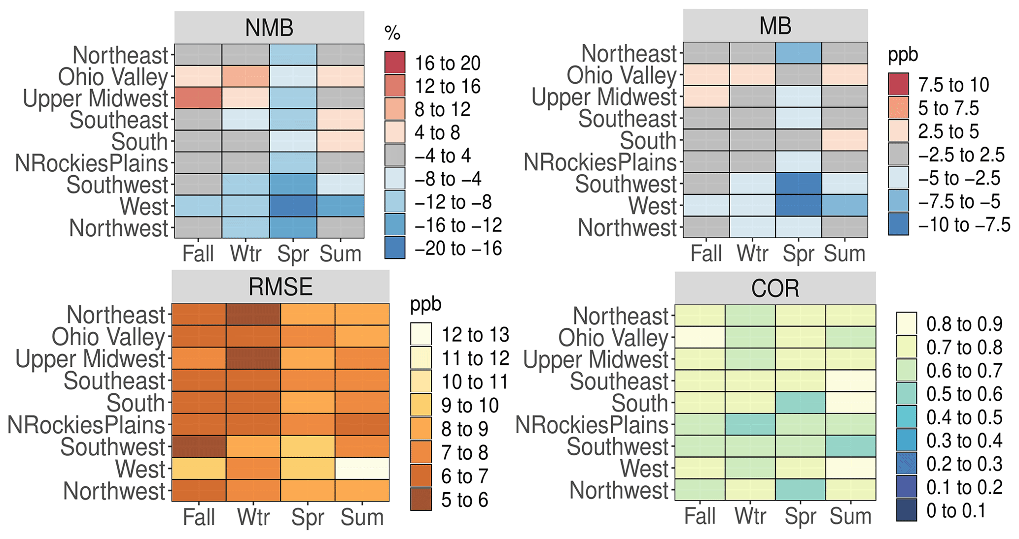
Figure 1NMB (%), MB (ppbv), RMSE (ppbv), and Pearson correlation coefficient values for MDA8 O3 for all AQS sites based on season and NOAA climate region for the CMAQ521 simulation.
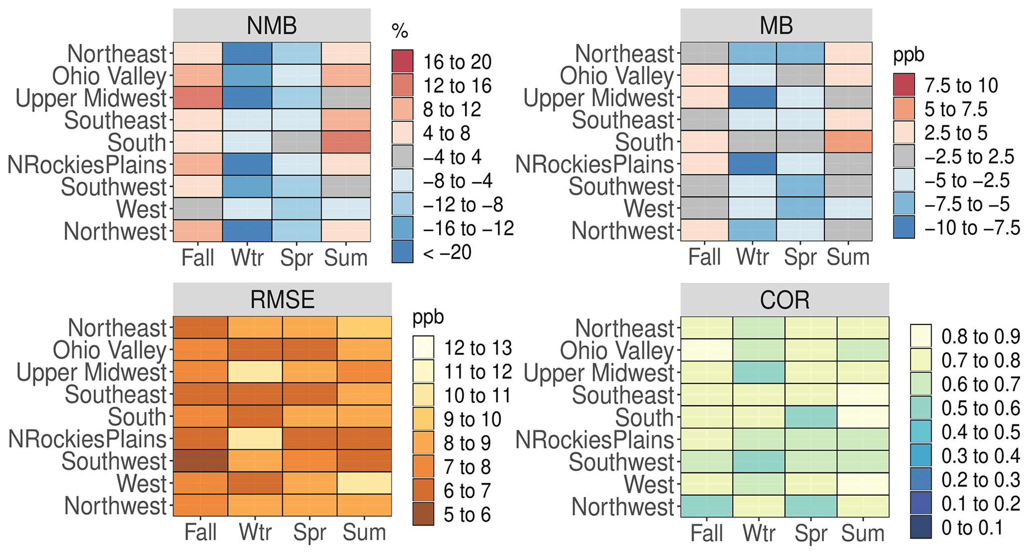
Figure 2NMB (%), MB (ppbv), RMSE (ppbv), and Pearson correlation coefficient values for MDA8 O3 for all AQS sites based on season and NOAA climate region for the CMAQ531_WRF411_M3Dry_BiDi simulation.
Figure 1 highlights the relatively large, widespread underestimation of O3 in winter and slightly smaller underestimation in spring for all regions with CMAQ521, while outside of spring MDA8 O3 is overestimated, particularly in the Ohio Valley and Upper Midwest regions. In the CMAQ531 simulation (Fig. 2), the large wintertime underestimation is largely eliminated, as are the overestimations in summer and fall. However, the underestimation in spring increases compared to the CMAQ521 simulation. Analysis of the seasonal diurnal hourly O3 trends (Figs. S8–S11) shows that in winter all hours have higher O3 with CMAQ531, improving the bias throughout much of the daytime hours but increasing the bias overnight compared to CMAQ521. The opposite trend occurs in spring, with O3 lower for all hours with CMAQ531, increasing bias throughout the day. Similarly, O3 is lower for all hours in the summer and fall with CMAQ531; however, this reduces the bias for most hours (except in the late afternoon and early evening in summer).
Underestimated O3 from the lateral BCs (discussed in more detail in Sect. 4.3) likely contributes strongly to the large springtime and smaller wintertime underestimation of MDA8 O3. Sarwar et al. (2019) showed that for a 2006 HCMAQ simulation CMAQ underestimated O3 mixing ratios at CASTNet sites (which better represent long-range-transported (LRT) O3) in spring and early summer, while a similar analysis for the HCMAQ53_M3Dry (and HCMAQ53_STAGE) simulation shows a relatively large (5.0–8.0 ppbv monthly average) underestimation O3 for CASTNet sites for March through June. Since springtime O3 at the majority of the rural CASTNET monitor locations is likely driven by LRT O3, this underestimate is likely associated with the underestimation in the large-scale O3 distributions in the lower troposphere of the HCMAQ simulations used in this analyses, which subsequently is influenced by uncertainties in global emission estimates, representation of O3 depletion in LRT air masses as they traverse large oceanic regions, and representation of stratosphere–troposphere exchange processes. This hypothesis is supported by comparisons of tropospheric O3 mixing ratios from the HCMAQ53_M3Dry to ozonesonde observations from 20 World Ozone and Ultraviolet Radiation Data Centre (WOUDC) sites, which shows that O3 is consistently underestimated by 20–40 ppbv in the mid-troposphere to upper troposphere (250–100 hPa) at most sites in spring (Figs. S3–S7). Overall, MDA8 O3 bias is improved outside of spring in the CMAQ531 simulation versus CMAQ521, largely due to improvements in the representation of O3 dry deposition in CMAQ531 and the more advanced WRF simulation (discussed in more detail in subsequent sections).
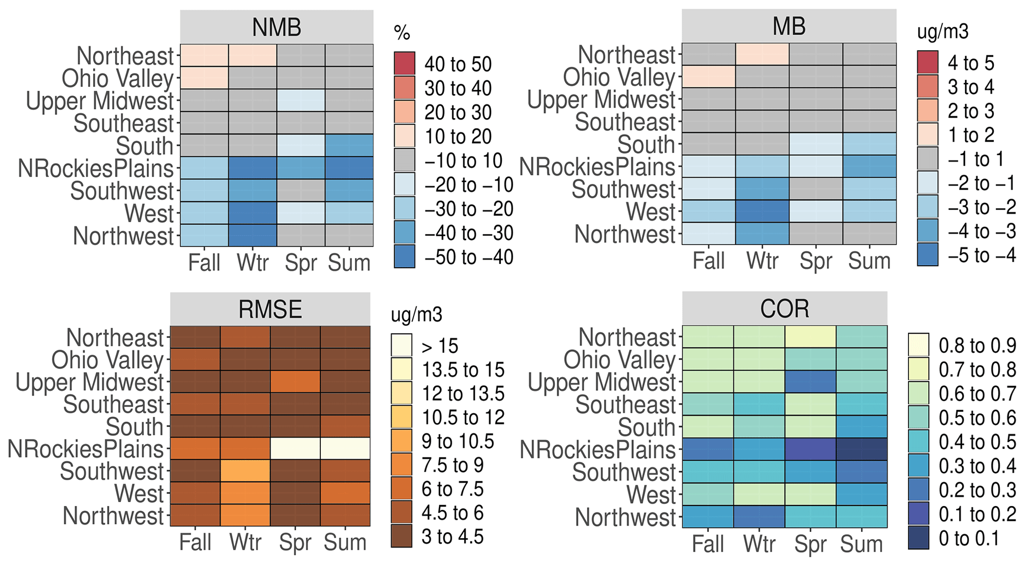
Figure 3NMB (%), MB (µg m−3), RMSE (µg m−3), and Pearson correlation coefficient (COR) values for daily average PM2.5 for all AQS sites based on season and NOAA climate region for the CMAQ521 simulation.

Figure 4NMB (%), MB (µg m−3), RMSE (µg m−3), and Pearson correlation coefficient (COR) values for daily average PM2.5 for all AQS sites based on season and NOAA climate region for the CMAQ531_WRF411_M3Dry_BiDi simulation.
Figures 3 and 4 highlight a general underestimation of PM2.5 in the western US for the both the CMAQ521 and CMAQ531 simulations, respectively. These underestimates are largely attributed to deficiencies in the meteorology simulated by WRF, which did not reproduce the strong wintertime inversions that occur in the western US; higher-resolution simulations may better resolve cold pools in the complex terrain in those regions (Kelly et al., 2019). PM2.5 in the eastern US is mostly unbiased throughout the year in both simulations, with higher correlation and lower RMSE than the western US regions. The diurnal trend in hourly PM2.5 in winter (Fig. S12) is comparable between CMAQ521 and CMAQ531, while in the spring the daytime PM2.5 underestimation is slightly greater (∼0.5 µg m−3) with CMAQ531 (Fig. S13). The nighttime underestimation in summer (Fig. S14) and fall (Fig. S15) improves with CMAQ531, while there is little difference in PM2.5 concentrations between the two simulations during the daytime. Overall, the PM2.5 in the CMAQ521 and CMAQ531 simulations has similar bias, error, and correlation, but there are some notable differences in the performance of the speciated PM2.5 components.
Organic carbon is overestimated in most regions in the CMAQ521 simulation (Figs. S16–S21), particularly in the winter and spring, where overestimations exceed 0.8 µg m−3 in many regions. There are also relatively large underestimations of OC in the West region in winter and the Northern Rockies and Plains region in spring and summer in the CMAQ521 simulation. In the CMAQ531 simulation, almost all the large overestimations and underestimations are eliminated, and the smaller overestimations are significantly reduced. Organic carbon remains overestimated in the Northeast, Ohio Valley, and Upper Midwest regions in spring in the CMAQ531 simulation, with smaller overestimates in the other seasons and slight underestimate (<0.4 µg m−3) in the Northern Rockies and Plains region in spring and summer. The underestimation of OC (SOA) in summer in the southeastern US noted in previous version of CMAQ (Appel et al., 2017; Murphy et al., 2017; Xu et al., 2018; Zhang et al., 2018) has been eliminated in CMAQ531 and replaced with a small overestimation. The reasons for the dramatic improvement in OC performance in the CMAQ531 simulation are discussed in detail in Sect. 4.2. Elemental carbon (EC) is generally unbiased in CMAQ521 simulation (Figs. S22–S27) except in the western US, particularly the Northwest region, where EC is overestimated at CSN sites by 0.4–1.0 µg m−3. The large seasonal overestimation of EC in the Northwest region is significantly reduced or eliminated in the CMAQ531 simulation, along with several of the larger RMSE values.
Particulate NO and TNO3 are underestimated for most seasons and regions (Figs. S28–S35) in the CMAQ521 simulation, with the largest underestimation in the western US in spring and summer. There is also a notable overestimation of NO in the Northwest region, particularly in the spring and summer. However, even the largest underestimations and overestimations by percent value (NMB) are still relatively small in absolute value (MB ±0.4 µg m−3). Particulate NO continues to be underestimated for many regions in the CMAQ531 simulation; however, the prior overestimation in the Northwest region is eliminated. The difference in NO between the two simulations is likely largely driven by the implementation of BiDi in the CMAQ531 simulation, along with smaller differences due to some of the other updates to the modeling system. Performance for particulate SO is generally good for most regions and seasons for both the CMAQ521 and CMAQ531 simulations (Figs. S36–S43), except in the Northwest region where NMB values exceed 40 % throughout the year (however MB values are <0.4 µg m−3) in both simulations. Particulate SO concentrations increase slightly in the CMAQ531 simulation, improving the underestimations in CMAQ521 but increasing the overestimations. Overall, however, the difference in SO concentrations between the two simulations is relatively small and would not have a large impact on the difference in total PM2.5 performance between the two simulations.
Figures S44–S47 show the SO2 performance for the two CMAQ simulations, which indicates similar performance for SO2 for the two simulations as well, with slightly higher SO2 mixing ratios indicated in the CMAQ531 simulation, particularly in the eastern US regions in the winter. However, as with SO, these differences have small absolute values, with very little effect on MB. Finally, the performance for NOx (Figs. S48–S49) is also very similar between CMAQ521 and CMAQ531, and the only notable difference is a larger underestimation (but reduced RMSE) of NOx in the Northwest region in the CMAQ531 simulation.
4.2 Impact of science updates in CMAQ version 5.3
Here we compare results between a CMAQ521 simulation and several similarly configured CMAQ531 simulations to highlight the impact of specific science updates in CMAQ531. All simulations presented in this section (see Table 1) utilize the same 2016 v1 EMP data, WRF38 meteorology, and M3Dry deposition model. To represent the science and system updates made in CMAQ531, three CMAQ531 simulations with slightly different configurations are presented in this section. The first simulation uses CMAQ531 without BiDi enabled and with the application of PCSOA to RWC (CMAQ531_WRF38_M3Dry_noBiDi_RWC). This simulation most closely mimics the configuration of the CMAQ521 simulation (specifically no BiDi and with PCSOA applied to RWC) and is intended to isolate the impact of the science updates in CMAQ53. The second CMAQ531 simulation removes the application of PCSOA to RWC using the DESID module and represents how PCSOA was intended to be applied in the model (CMAQ531_WRF38_M3Dry_noBidi). The final CMAQ531 simulation in this section builds upon the second simulation by exercising the M3Dry BiDi option in the model (CMAQ531_WRF38_M3Dry_BiDi), highlighting the impact of that process on model-estimated concentrations. There are two additional CMAQ531 simulations using WRF411: one with M3Dry (CMAQ531_WRF411_M3Dry_BiDi) presented in Sect. 4.3 and one with STAGE (CMAQ531_WRF411_STAGE_BiDi) presented in Sect. 4.4.

Figure 5Time series of monthly average MDA8 O3 bias (ppbv) compared against all AQS sites. Note that the blue, green, and purple lines all fall very close to one another.
Figure 5 presents a time series of monthly average MDA8 O3 bias for all AQS sites within the 12 km domain for the CMAQ521 and five CMAQ531 simulations. Similar time series plots for MDA8 O3 mixing ratio, RMSE, and COR, along with spatial plots of seasonal MDA8 O3 bias for the CMAQ521 and CMAQ531 simulations, are shown in Figs. S50–S54. A comparison of MDA8 O3 time series plots stratified by rural, suburban, and urban sites (as specified by AQS) showed very similar values and trends to the time series of all sites (Fig. S3). Other than the winter months (December, January, February), average MDA8 O3 is consistently lower by approximately 1.0–2.0 ppbv in the three CMAQ531 simulations that use WRF38 versus the CMAQ521 simulation, and there is little difference between the three CMAQ531 simulations, indicating that removing the application of PCSOA on RWC and enabling BiDi (as expected) minimally affects monthly average O3 mixing ratios. While summertime and wintertime bias (Fig. S50) and RMSE (Fig. S51) considerably improve in the CMAQ531 simulations, COR (Fig. S52) is slightly higher throughout the year in the CMAQ521 simulation. The lower O3 mixing ratios outside of winter are primarily due to the update to Rg (O3) in CMAQ531, which decreases the resistance of O3 dry deposition to soil, thereby increasing O3 dry deposition and decreasing ambient O3 mixing ratios. In the winter, the decrease in O3 dry deposition to snow in CMAQ531 results in higher average ambient O3 mixing ratios due to more prevalent snow cover.
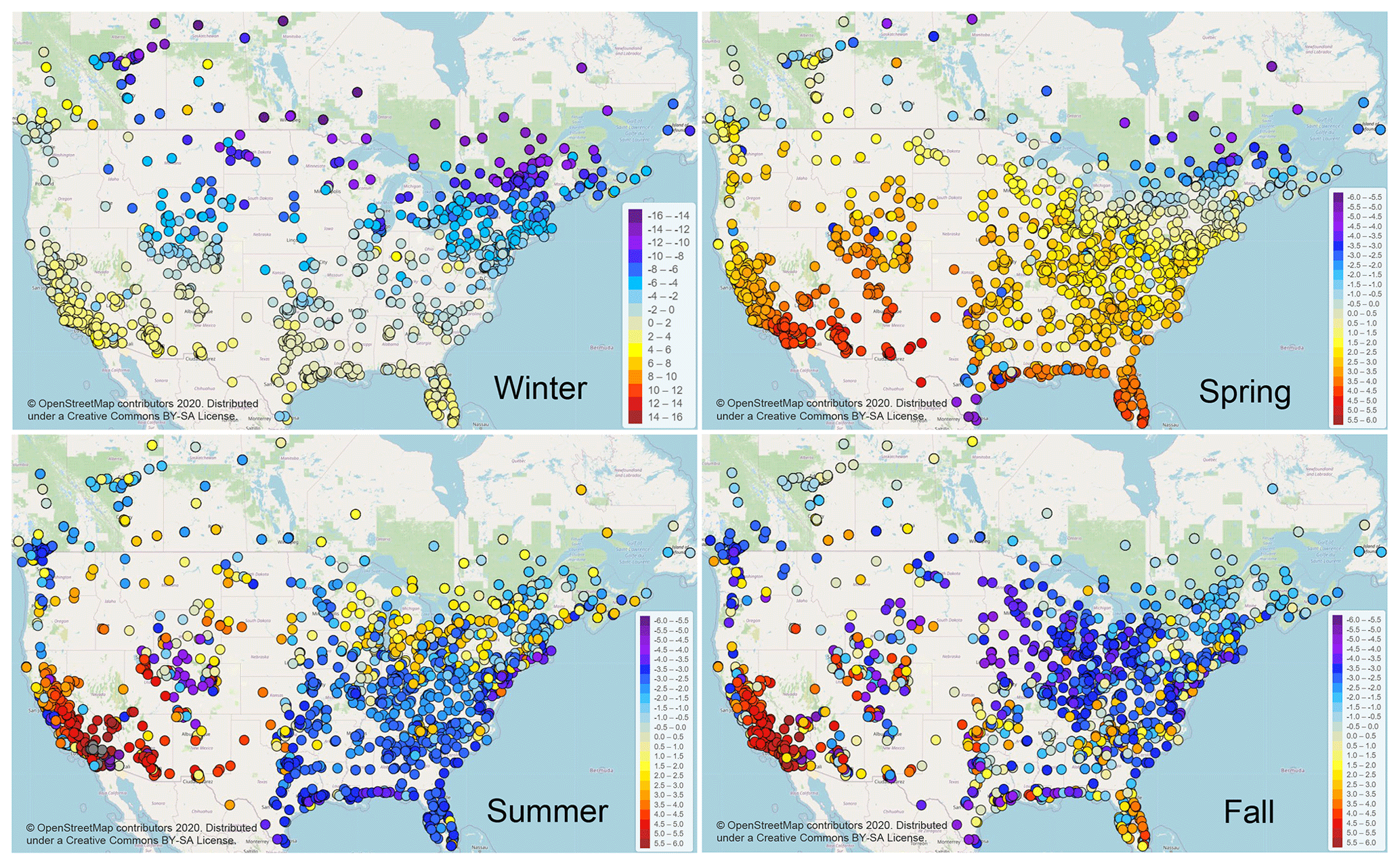
Figure 6Seasonal average MDA8 O3 absolute bias difference (ppbv) between the CMAQ521 and CMAQ531_WRF38_M3Dry_BiDi simulations for all AQS and NAPS sites. Cool shading (negative values) indicates a smaller bias in the CMAQ531_WRF38_M3Dry_BiDi simulation, warm colors (positive values) indicates a smaller bias in the CMAQ521 simulation. Note that the scale is different for the winter season. Grey shading indicates values beyond the range of the scale.

This latitudinal effect on O3 mixing ratios from snow cover is apparent in Fig. 6, which presents the difference in seasonal average MDA8 O3 absolute bias between the CMAQ521 simulation and the CMAQ531_WRF38_M3Dry_BiDi simulation. In winter, sites in the US northern latitudes and Canada indicate a seasonal average reduction in MDA8 O3 bias of 10 ppbv or more with CMAQ531. Sites in the lower latitudes show little change in bias, with some sites in the southern US showing a slight increase in bias with CMAQ531. In spring (March, April, May), MDA8 O3 bias is broadly higher with CMAQ531, with bias increasing from north (where the update of deposition to snow still results in lower bias) to south, where seasonal average biases are higher by up to 4.0–5.0 ppbv.
In summer (June, July, August), bias is lower in the CMAQ531_WRF38_M3Dry_BiDi simulation by 2.0–4.0 ppbv across much of the US and Canada, with the largest exception in the southwestern US (including California) where the bias increases by 3.0–6.0 ppbv at many sites, primarily due to lower ambient O3 mixing ratios from increased O3 dry deposition. Previous studies have shown that mean O3 is often overestimated by CMAQ in the summer (except in California), so the broad decrease in O3 with CMAQ531 reduces the bias at most sites but worsens underestimation in California. The pattern in fall (September, October, November) is similar to summer, with a large, broad decrease in bias for most sites outside of the southwestern US with CMAQ531. Sites in southern Florida indicate higher bias with CMAQ531 (3.0–4.0 ppbv), as do some other sites in the southeastern US. Overall, outside of spring, MDA8 O3 bias is generally lower with CMAQ531 (particularly in the eastern US), with the noted exception of increased negative bias in California.
Figure 7 presents a time series of monthly average PM2.5 bias for all AQS sites within the 12 km domain for the CMAQ521 and five CMAQ531 simulations. Similar time series plots for PM2.5 concentration, RMSE, and COR, along with spatial plots of seasonal PM2.5 bias for the CMAQ521 and CMAQ531 simulations are shown in Figs. S55–S59. Comparing first the CMAQ521 simulation and the CMAQ531_WRF38_M3Dry_noBiDi_RWC simulation, PM2.5 is underestimated throughout the year with CMAQ521, with monthly average biases ranging from approximately zero to 1.5 µg m−3 and the largest underestimations in the summer. Concentrations of PM2.5 in the CMAQ531_WRF38_M3Dry_noBiDi simulation are significantly higher (0.5–1.2 µg m−3 monthly average) than the CMAQ521 simulation in winter (December, January, February) and slightly higher in the late summer through early fall (August, September, October). The higher PM2.5 concentrations with CMAQ531 are primarily due to greater SOA from monoterpene oxidation from more abundant oxidants (e.g., O3, OH−) in the winter in CMAQ531, which results in relatively large increases in OC (0.5–2.0 µg m−3 monthly average) and non-carbon organic matter (NCOM; organic matter minus OC) (0.5–1.0 µg m−3 monthly average), primarily over the eastern half of the US (not shown). When PCSOA application to RWC sources is removed (CMAQ531_WRF38_M3Dry_noBiDi), PM2.5 concentrations are significantly reduced in the winter compared to the simulation with PCSOA applied to RWC sources and are slightly higher than but much closer to the monthly average PM2.5 concentrations from the CMAQ521 simulation. The largest decrease in PM2.5 occurs in the winter and spring, when monthly average PM2.5 concentrations decrease by approximately 0.5–1.2 µg m−3 (essentially offsetting the increase in PM2.5 due to the increased oxidants in winter). Changes in monthly average PM2.5 concentrations in summer and early fall are generally less than 0.25 µg m−3, indicating little impact from removing the application of PCSOA on RWC sources outside of winter and spring.
Enabling BiDi (CMAQ531_WRF38_M3Dry_BiDi) slightly increases PM2.5 concentrations throughout the year (Figs. 7 and S55), which is expected given that the effect of BiDi is generally localized to areas with high amounts of NH3 (e.g., crop lands), and thus the highly spatially and temporally averaged time series plots cannot highlight the heterogenous impact of BiDi. Areas with large agricultural production requiring frequent fertilization, such as the San Joaquin Valley (SJV) in California and the Midwest US, are expected to show a much larger impact from implementation of the BiDi option (Pleim et al., 2019).
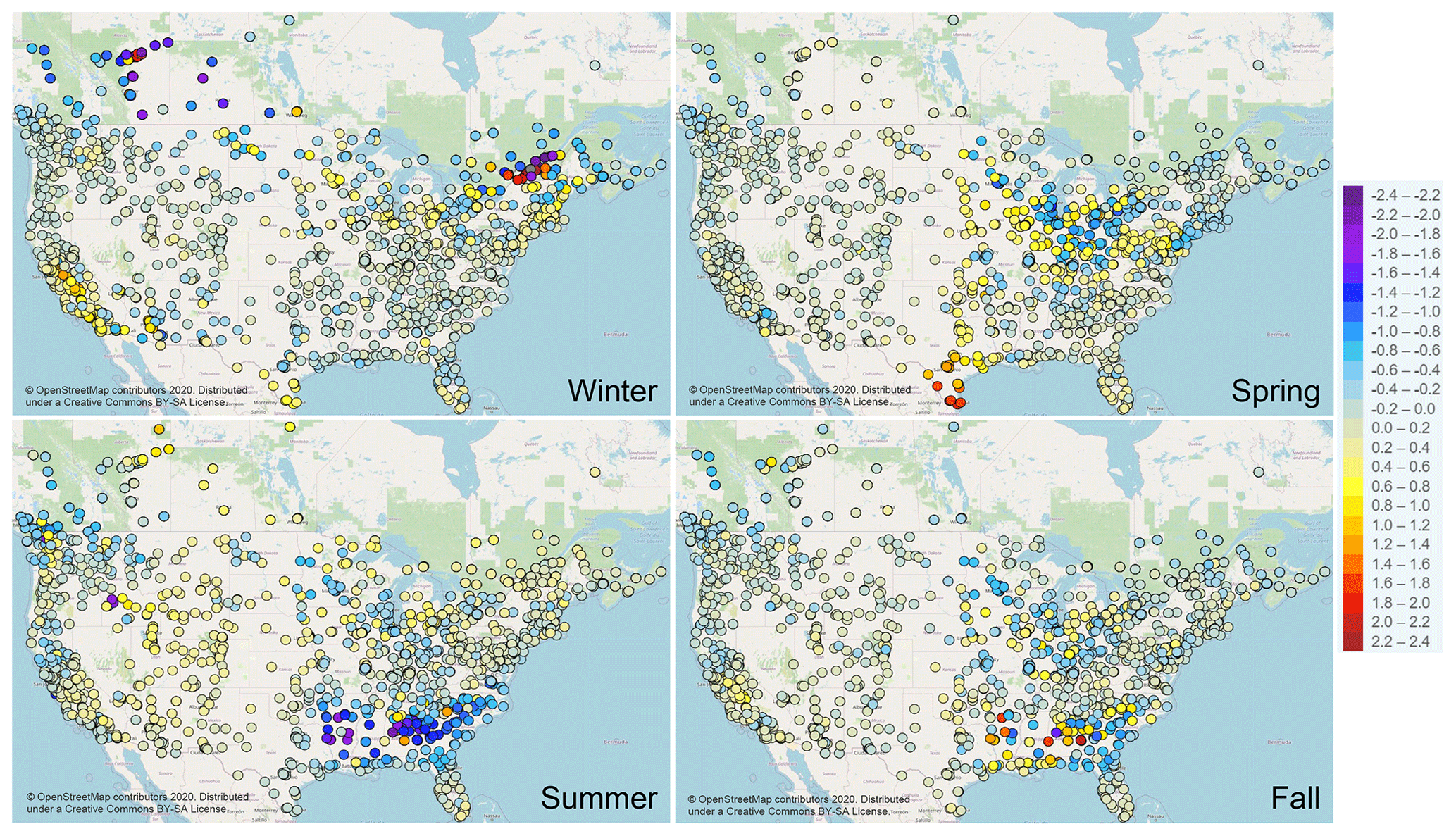
Figure 8Seasonal average PM2.5 absolute bias difference (µg m−3) between the CMAQ521 and CMAQ531_WRF38_M3Dry_BiDi simulations for all AQS and NAPS sites. Cool shading (negative values) indicate smaller bias in the CMAQ531_WRF38_M3Dry_BiDi simulation, warm colors (positive values) indicate smaller bias in the CMAQ521 simulation. Grey shading indicates values beyond the range of the scale.
Figure 8 shows the difference in seasonal average PM2.5 absolute bias between the CMAQ521 simulation and the CMAQ531_WRF38_M3Dry_BiDi simulation for AQS and NAPS sites. For winter, the change in bias is relatively small for most of the sites located in the US, except in the southwestern US and California, where the bias is notably higher with CMAQ531, and in sites across the northern portion of the US where the change in bias (both positive and negative) tends to be higher than sites in other parts of the US Conversely, the NAPS sites in Canada indicate a large widespread decrease in PM2.5 bias with CMAQ531, which may result from the Canadian emission inventory containing RWC emissions and which leads to a larger impact on PM2.5 from the updates in CMAQ531 (RWC emissions were treated separately from the other gridded emissions in the US emission inventory in the CMAQ531 simulations). In spring, the largest differences in bias occur for sites in the upper Midwest and into the northeastern US, particularly for sites in and around the Great Lakes region, where both large increases and decreases in bias occur, and through the Midwest states stretching down to Texas, where the bias is generally higher with CMAQ531.
In summer, the most notable difference between the two simulations is a widespread, large decrease in bias in the southeastern US in the CMAQ531_WRF38_M3Dry_BiDi simulation, largely the result of increased PM2.5 from monoterpene SOA from the new AERO7 module. In late summer and early fall, total PM2.5 increases primarily in areas rich in vegetation (e.g., the southeastern US) due to increased monoterpene oxidation products with secondary effects due to water uptake to particles in AERO7. In the southeastern US, the increase in PM2.5 in summertime (0.75–3.0 µg m−3 monthly average) is primarily driven by an increase in OC (with smaller increases during other times of year due to lower monoterpene emissions and lower oxidants in other seasons). Including additional water uptake to hydrophilic organic species results in small decreases in total PM2.5 due to changes in the size distribution that increase dry deposition. Bias is also broadly lower in the simulation using CMAQv531 across the upper Midwest, northwestern US, and into southwestern Canada, while bias increases slightly across the Rocky Mountain region and parts of the upper Midwest US and southern Canada. Similar to summer, there is a relatively large decrease in PM2.5 bias in fall across the southwestern US, juxtaposed with several sites where bias increases. There are also relatively large changes in bias through the upper Midwest US and broad (slightly) lower bias along the west coast states, with higher bias in the SJV of California.

Figure 9Seasonal stacked bar plots of speciated PM2.5 (µg m−3) for AQS sites. The height of the bar represents the total PM2.5 concentration. Refer to Table 1 for more details about the simulation configurations.
Figure 9 presents seasonal stacked bar plots of observed speciated PM2.5 for all sites in AQS that reported speciated data (includes both CSN and IMPROVE sites) and the corresponding simulated values from the various CMAQ simulations. The OTHR (“PM other”) species is calculated as a difference between the total measured and predicted PM2.5 and the sum of the individual measured and predicted PM2.5 species. There is generally good performance for SO, NO, and NH bias throughout the year, with all three species nearly unbiased in winter and fall and slightly underestimated (0.25–0.5 µg m−3) in spring and summer. An overestimation in OC with CMAQ521 in winter, spring, and fall is reduced in the CMAQ531 simulations, although OC is still overestimated compared to the observations. Total PM2.5 is underestimated in summer, driven primarily by an underestimation of OTHR, with smaller underestimations of SO4, NO, and NH4+ also contributing to the underestimation. More work is needed to better classify the observed “PM other” mass so that the model estimates can be improved.
Overall, while the monthly average PM2.5 concentrations are similar between CMAQ521 and CMAQ531, there are some relatively large regional and seasonal differences between the two versions of the model. In addition, while the averaged PM2.5 concentrations are overall comparable between the two versions of the model, the underlying science has been improved in CMAQ531.
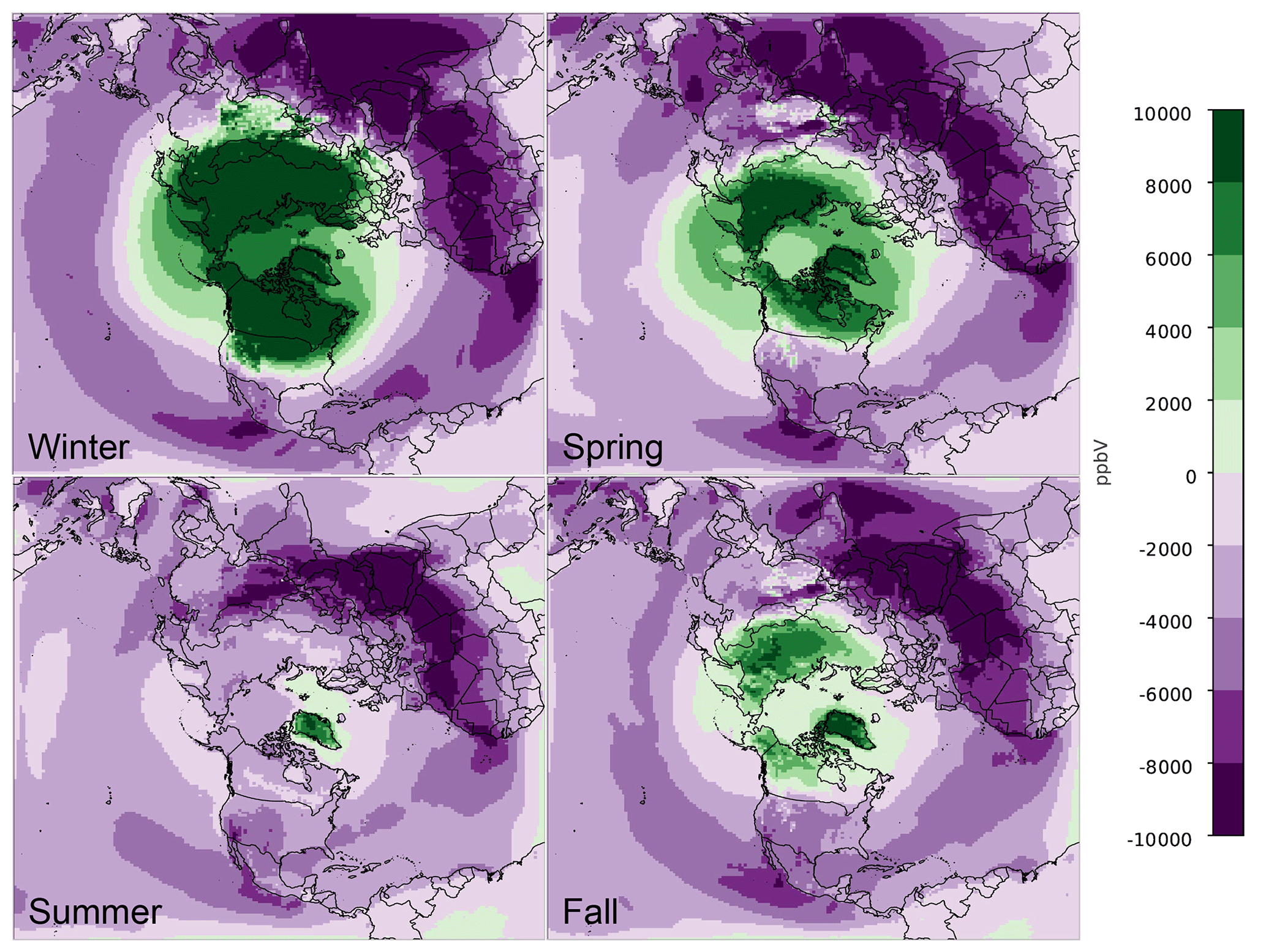
Figure 10Difference in seasonal average surface O3 mixing ratios (ppbv; all hours) between HCMAQ521 and HCMAQ531_M3Dry simulations (HCMAQ531_M3Dry – HCMAQ521). Green shading indicates higher O3 mixing ratios and purple shading indicates lower O3 mixing ratios in the HCMAQ531_M3Dry simulation.
4.3 HCMAQ simulations and impact on BCs
The analysis presented in Sect. 4.1 focused on isolating the impacts of the science updates in CMAQ53 on model performance, including updating the science in the lateral BCs by transitioning from BCs created from a HCMAQ521 simulation to those created from a HCMAQ53 simulation. Lateral BCs increasingly influence pollutant concentrations in the regional simulation, as locally emitted pollutants across the US have declined over time. Pollutants specified in the middle and upper troposphere in the BCs can be advected long distances and interact with locally emitted pollutants to alter surface and boundary layer pollutant concentrations (Hogrefe et al., 2018). As described in Sect. 3.3, BCs for the regional CMAQ simulations were derived from a HCMAQ521 simulation (used for the regional CMAQ521 simulation) and from a HCMAQ53 simulation using the M3Dry deposition model (used for the CMAQ531 M3Dry simulations). In this section we briefly compare the operational performance of the two HCMAQ simulations and examine how differences in HCMAQ model performance influence the BCs used in the regional-scale CMAQ simulations.
Figure 10 shows the difference in seasonal average surface O3 (all hours) between the HCMAQ521 and HCMAQ53_M3Dry simulations. Analogous to the regional CMAQ simulations, O3 mixing ratios are consistently higher (10–20 ppbv) in the HCMAQ53_M3Dry simulation in the winter and spring over the higher latitudes of North America where snow cover is more prevalent. In the middle and lower latitudes, O3 mixing ratios are generally lower in the HCMAQ53_M3Dry simulation by approximately 0.0–5.0 ppbv in winter and 5.0–10 ppbv in fall, primarily due to the updates to bromine and iodine chemistry reducing O3 mixing ratios over the oceans. These differences consistently reduce O3 in the middle to lower latitudes with CMAQ53-derived lateral BCs compared to CMAQ521-derived BCs, which contributes to reducing MDA8 O3 in spring, summer, and fall in the regional CMAQ531 simulations. Although not shown in Fig. 6, the lower O3 in the HCMAQ53_M3Dry simulation extends through the lower troposphere (Sarwar et al., 2019). The ozonesondes presented in Figs. S3–S8 also show lower O3 throughout the troposphere at many sites in the HCMAQ53 simulation.
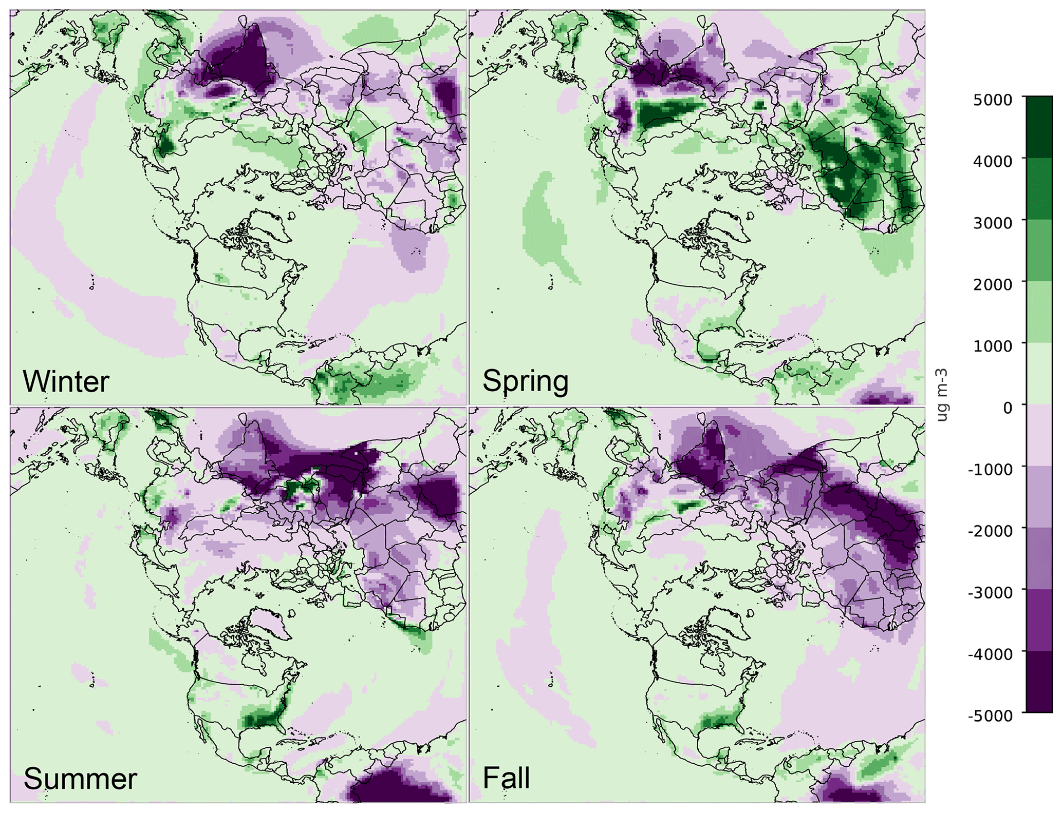
Figure 11Difference in seasonal average surface PM2.5 concentrations (µg m−3; all hours) between the HCMAQ521 and HCMAQ531_M3Dry simulations (HCMAQ531_M3Dry – HCMAQ521). Green shading indicates higher PM2.5 concentrations and purple shading indicates lower PM2.5 concentrations with the HCMAQ531_M3Dry simulation.
Figure 11 shows the difference in seasonal average surface PM2.5 (all hours) between the HCMAQ521 and HCMAQ53_M3Dry simulations. The pattern mimics that in the regional CMAQ simulations, with a relatively small difference over and around North America in winter and larger differences in spring, summer, and fall. In spring, the differences start to reveal higher PM2.5 in the southeastern US and slightly lower PM2.5 in the west. In summer, there is a large increase in PM2.5 in the southeast and north along the east coast of the US and a small increase in the west with CMAQ53. In fall, the increase in PM2.5 in the HCMAQ53_M3Dry simulation is still present in the southeastern US. Outside the conterminous US, the difference in PM2.5 is relatively small between the two HCMAQ simulations, suggesting that differences in simulated PM2.5 concentrations in the regional CMAQ simulations for the US and Canada are minimally influenced by differences between the BCs.
4.4 Impact of updating meteorology
Meteorology is a critical component of air quality modeling, as changes in meteorology have the potential to drastically alter pollutant concentrations over large temporal and spatial scales, consequently impacting overall performance of the air quality modeling system. Meteorology models are frequently updated to improve underlying science, add functionality, and address errors in the model. As described in Sect. 3.1, two versions of WRF (WRF38 and WRF411) were used during the development and testing of the CMAQ53 modeling system. In this section we compare the operational performance between two CMAQ531 simulations with the same configuration, except that one is driven using WRF38 (SVC) inputs and the other is driven using WRF411 (HVC and updated land-surface parameters); the relevant differences are described in Sect. 3.1. Although the HCMAQ simulation from which BCs are derived was not run using WRF411, they have been reprocessed to the WRF HVC to align with the vertical coordinate of the CMAQ simulation that was run using WRF411. This reprocessing results in only a very small difference between BCs using the SVC and HVC. Note that versions of CMAQ prior to 5.3 and versions of MCIP prior to 5.0 are not compatible with the WRF HVC.
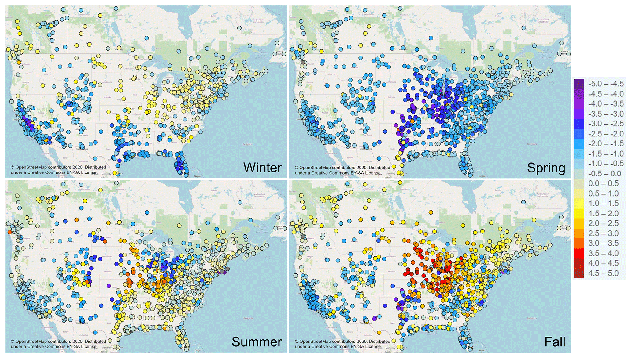
Figure 12Seasonal average MDA8 O3 absolute bias difference (ppbv) between the CMAQ531_WRF38_M3Dry_BiDi and CMAQ531_WRF411_M3Dry_BiDi simulations for all AQS and NAPS sites to highlight the impact of the updated WRF version. Cool shading (negative values) indicates smaller bias in the CMAQ531_WRF411_M3Dry_BiDi simulation, and warm colors (positive values) indicate smaller bias in the CMAQ531_WRF38_M3Dry_BiDi simulation.
MDA8 O3 is consistently higher throughout the year in the simulation using WRF411 (CMAQ531_WRF411_M3Dry_BiDi), with the largest increase occurring in spring and fall when monthly averaged MDA8 O3 is approximately 1.5 ppbv higher on average (Fig. 1). The increase is slightly smaller (1.0–1.5 ppbv) in winter and summer. This increase in O3 generally reduces bias in the simulation using WRF411 throughout most of the year, except during warmer months (July, August, September) when bias increases, as MDA8 O3 is overestimated on average in summer. Figure 12 shows seasonal average spatial plots of the change in MDA8 O3 absolute bias at all AQS and NAPS sites. Sites in the southern US (particularly along coastal areas), California, and the Northwest region show the largest reduction in bias in winter, while sites in the upper Midwest show the largest increase in bias. In spring, almost all the sites indicate some reduction in bias with WRF411, except along the southern tip of Texas and scattered sites in the Northwest region. In summer, the pattern shifts, with sites in the western US and Great Lakes region showing the largest decrease in bias, while sites in the upper Midwest still indicate an increase in bias with WRF411. Fall has the largest mixed signal in bias change, with sites in the southern US and California indicating a decrease in bias, while sites in the upper Midwest and Northeast region indicate a relatively large increase.
These differences in O3 are likely driven by updates to the vegetation parameters used in WRF and their impact on the meteorological fields and the deposition in CMAQ. As explained in Sect. 3.1, the WRF411 simulations used vegetation parameters directly from MODIS satellite retrievals which result in generally lower values for VF and LAI, especially in most of western North America (Fig. S1). These differences not only affect the meteorological simulations but also the chemical surface fluxes (dry deposition and bidirectional fluxes) since these algorithms in CMAQ use the vegetation parameters from WRF (via the MCIP input files). The higher MDA8 O3 concentrations evident in the time series (Fig. 5) and spatial plot (Fig. 12) for the simulation using WRF411 are primarily due to reduced dry deposition of O3, as deposition to vegetation is generally greater than deposition to bare ground (Fig. S60). Thus, the lower VF and LAI from the WRF411 simulation result in lower O3 deposition velocities and therefore higher ambient concentrations. Also potentially contributing to the higher O3 mixing ratios with WRF411 are the systematically drier (lower precipitation) conditions with WRF411 versus WRF38 throughout the year, particularly in the central and eastern US, where WRF tends to underestimate the observed precipitation (Figs. S62–S65). The lower precipitation in WRF411 results in less O3 wet scavenging and may also reflect fewer fair-weather cumulus clouds, which would increase O3 photochemical production.
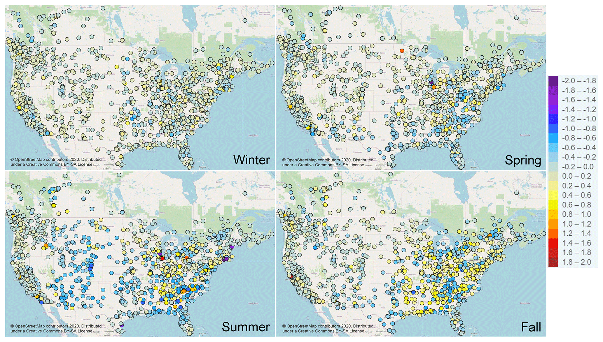
Figure 13Seasonal average PM2.5 absolute bias difference (µg m−3) between the CMAQ531_WRF38_M3Dry_BiDi and CMAQ531_WRF411_M3Dry_BiDi simulations for all AQS and NAPS sites to highlight the impact of the updated WRF version. Cool shading (negative values) indicates smaller bias in the CMAQ531_WRF411_M3Dry_BiDi simulation, and warm colors (positive values) indicate smaller bias in the CMAQ531_WRF38_M3Dry_BiDi simulation.
For PM2.5, transitioning from WRF38 to WRF411 is largely unremarkable. Apart from January and February, PM2.5 concentrations are consistently higher throughout the year in the simulation using WRF411, particularly in summer and fall when monthly average values increase by approximately 0.1–0.25 µg m−3 (Fig. 3). Figure 13 shows seasonal average spatial plots of the change in PM2.5 absolute bias between the two simulations. In winter, there are widespread changes in PM2.5 bias, while in spring sites in the southeastern and mid-Atlantic US show larger decreases in bias with WRF411 compared to sites across the rest of the country. In summer, sites in the eastern half of the US indicate the largest change in bias, while sites in the western half of the country generally show a small decrease in bias with WRF411. Finally, for fall, there is generally a decrease in bias with WRF411, particularly at sites in the southeastern US, lower Midwest, and Rocky Mountain regions. The differences in PM2.5 concentrations using both versions of WRF are likely attributed to a combination of the lower precipitation in WRF411 and the differences in vegetation parameters (Fig. S61). Drier conditions reduce aerosol growth, which reduces deposition velocities and settling velocities for the larger particles. The changes in vegetation parameters affect PM2.5 because, as noted above, the aerosol dry deposition model now has dependencies on LAI and VF.
4.5 Impact of STAGE and M3Dry deposition models
The final updates in CMAQ531 examined here are the updated M3Dry and new STAGE deposition models. Both deposition models originate from previous versions of the M3Dry model, which has a long history in CMAQ and CTMs (USEPA, 1994). However, the dry deposition algorithms in the updated M3Dry and STAGE models differ substantially in many of their resistance algorithms, which substantially alters simulated pollutant concentrations and depositions. The scientific differences between M3Dry and STAGE inhibit the ability to solely associate specific changes in species behavior with any aspect of either model. Here, CMAQ531 simulations are compared using the same configuration except for the deposition model (i.e., M3Dry or STAGE). To consistently represent air–surface exchange processes across scales, the lateral BCs for the regional M3Dry and STAGE simulations are generated from HCMAQ simulations configured with the corresponding deposition model.
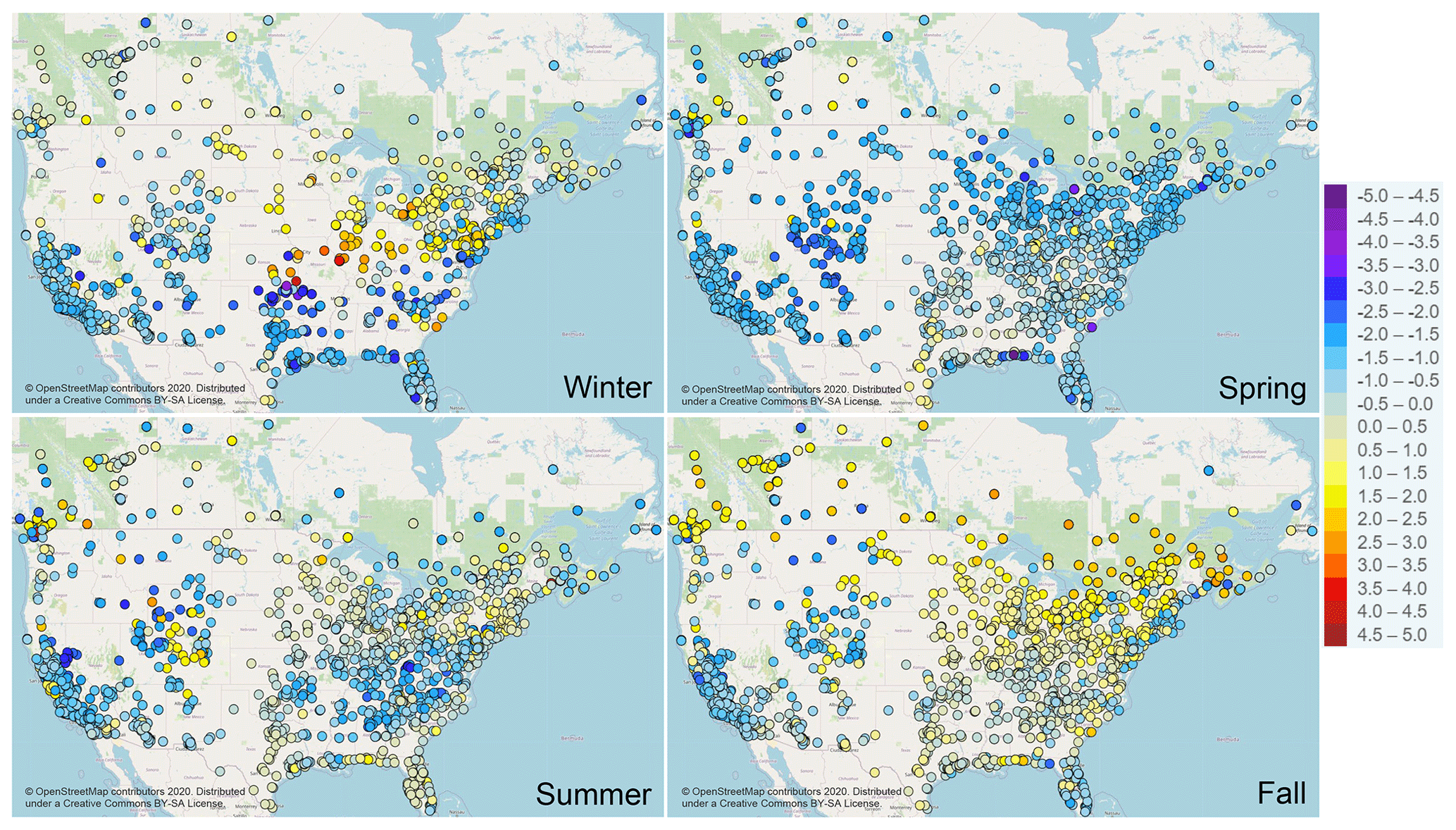
Figure 14Seasonal average MDA8 O3 absolute bias difference (ppbv) between CMAQ531_WRF411_M3Dry_BiDi and CMAQ531_WRF411_STAGE_BiDi simulations for all AQS and NAPS sites to highlight the impact of the M3Dry and STAGE deposition models. Cool shading (negative values) indicates smaller bias in the CMAQ531_WRF411_M3Dry_BiDi simulation, and warm colors (positive values) indicate smaller bias in the CMAQ531_WRF411_STAGE_BiDi simulation.
The time series of monthly average MDA8 O3 bias across all AQS sites for the M3Dry (CMAQ531_WRF411_M3Dry_BiDi) and STAGE (CMAQ531_WRF411_STAGE_BiDi) simulations are presented in Fig. 5. Aside from several warmer months (July, August, September), when both simulations have very similar performance, MDA8 O3 is consistently higher in the M3Dry simulation. In spring, monthly average MDA8 O3 mixing ratios are 1.0–1.5 ppbv higher in the M3Dry simulation, while in November and December mixing ratios are 1.5–2.0 ppbv higher. The higher mixing ratios in the M3Dry simulation improve overall performance for MDA8 O3 bias versus the STAGE simulation, as MDA8 O3 is broadly underestimated by CMAQ outside of summer. Figure 14 shows the difference in seasonal MDA8 O3 absolute bias between the M3Dry and STAGE simulations. For winter, the simulation using M3Dry shows improved (smaller) bias across most of the sites, except for the Upper Midwest region and near the Great Lakes, where the simulation using STAGE has smaller bias. In spring, almost all sites indicate smaller bias with M3Dry, while in summer the bias signal is generally mixed with no apparent pattern. In fall, the simulation using STAGE has smaller bias for sites across the northern portion of the US and Canada (note that sites in Canada are not included in the time series in Figs. 5 and 7), while the simulation using M3Dry has smaller bias for sites across the southern US and California. The generally higher O3 in the M3Dry simulation is likely a combination of both higher O3 in the regional simulation and higher O3 introduced from the lateral BCs.
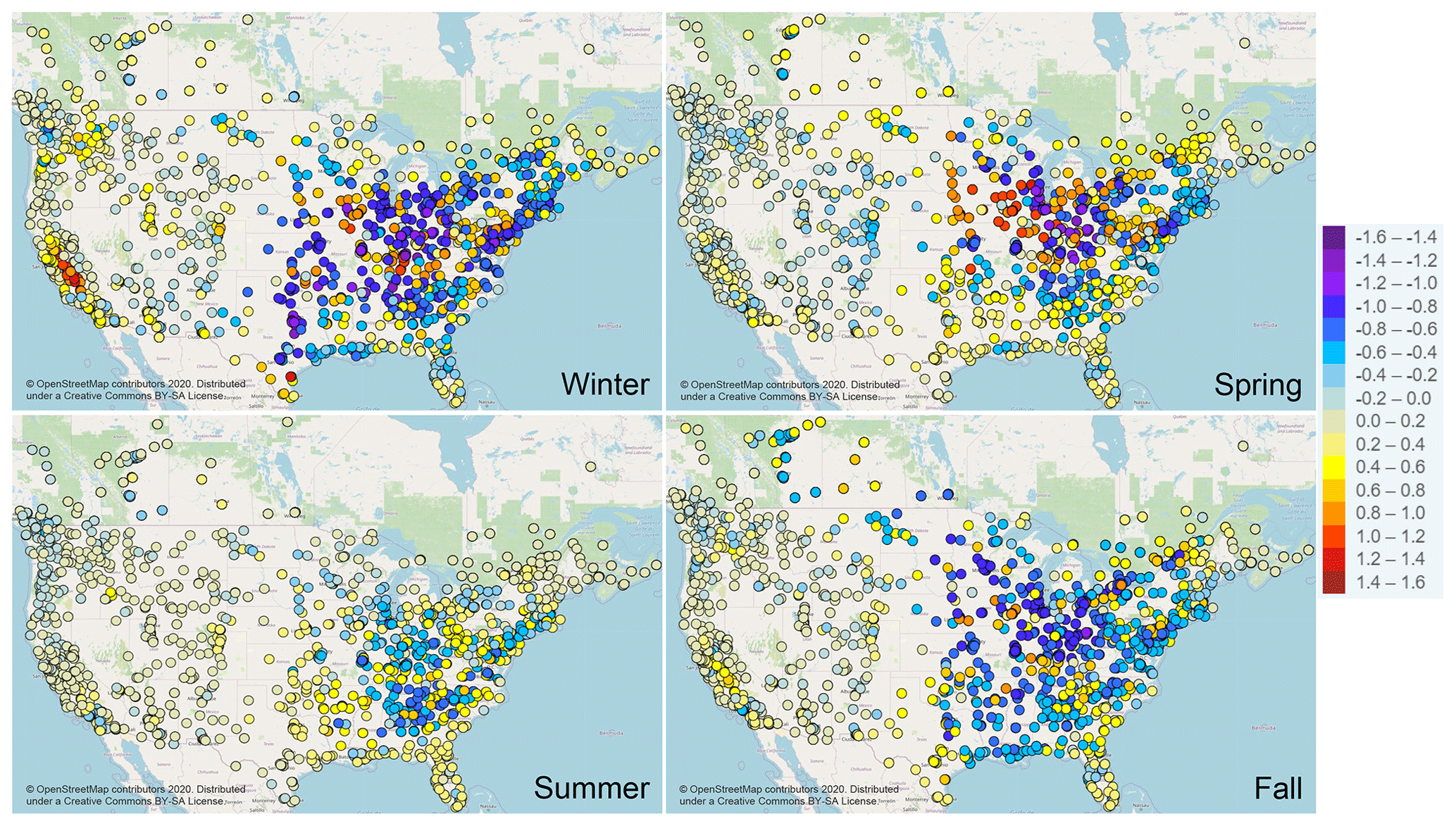
Figure 15Seasonal average PM2.5 absolute bias difference (µg m−3) between CMAQ531_WRF411_M3Dry_BiDi and CMAQ531_WRF411_STAGE_BiDi simulations for all AQS and NAPS sites to highlight the impact of the M3Dry and STAGE deposition models. Cool shading (negative values) indicates smaller bias in the CMAQ531_WRF411_M3Dry_BiDi simulation, and warm colors (positive values) indicate smaller bias in the CMAQ531_WRF411_STAGE_BiDi simulation.
For daily average PM2.5, the simulation using STAGE has consistently higher monthly average concentrations (approximately 0.25–0.75 µg m−3) throughout the year, which, except during April, September, and October, reduces bias (Fig. 5). For winter, sites in the eastern US generally have smaller bias with M3Dry while sites in the western US tend to have smaller bias with STAGE (Fig. 15). The pattern shifts slightly in spring and summer, with sites in the Great Lakes, the Northeast region, and the western US having smaller bias with M3Dry, while sites in the southern US and Canada have smaller bias with STAGE. In fall, sites in the northern US and Canada have smaller bias with STAGE, while sites in the southern and western US have smaller bias with M3Dry. Overall, the difference in bias for PM2.5 between the two deposition models is consistent throughout the year, with relatively similar patterns in bias regardless of season.
The consistently higher PM2.5 concentrations using the STAGE model are due to differences in the assumptions affecting deposition velocity to surfaces in the M3Dry and STAGE models. M3Dry uses a revised formulation of the dry deposition impaction term, and thus it integrates the effect of mode width in the Stokes number via the settling velocity rather than adjusting the impaction term magnitude directly, which intends to resolve the massive overprediction of deposition velocity for coarse-mode particles. In addition, the impaction term in M3Dry in CMAQ53 is based on Slinn (1982), while the Stokes number is based on Slinn (1982) and Giorgi (1986). In STAGE, the Stokes number for each vegetated land use type is calculated using the leaf geometry from Zhang et al. (2001), and a different form of the Stokes number is used for deposition to smooth surfaces, ground, and water. These different parameterizations implemented in M3Dry and STAGE lead to the different estimates for PM2.5 (and O3).

Figure 16Time series of monthly average observed and simulated NH3 concentrations (solid circle; µg m−3), bias (open square; µg m−3), RMSE (dotted solid circle; µg m−3), and Pearson correlation coefficient (dot-dashed solid stars) for all AMON sites for CMAQ531_WRF411_M3Dry_BiDi simulation (red) and CMAQ531_WRF411_STAGE_BiDi simulation (blue).
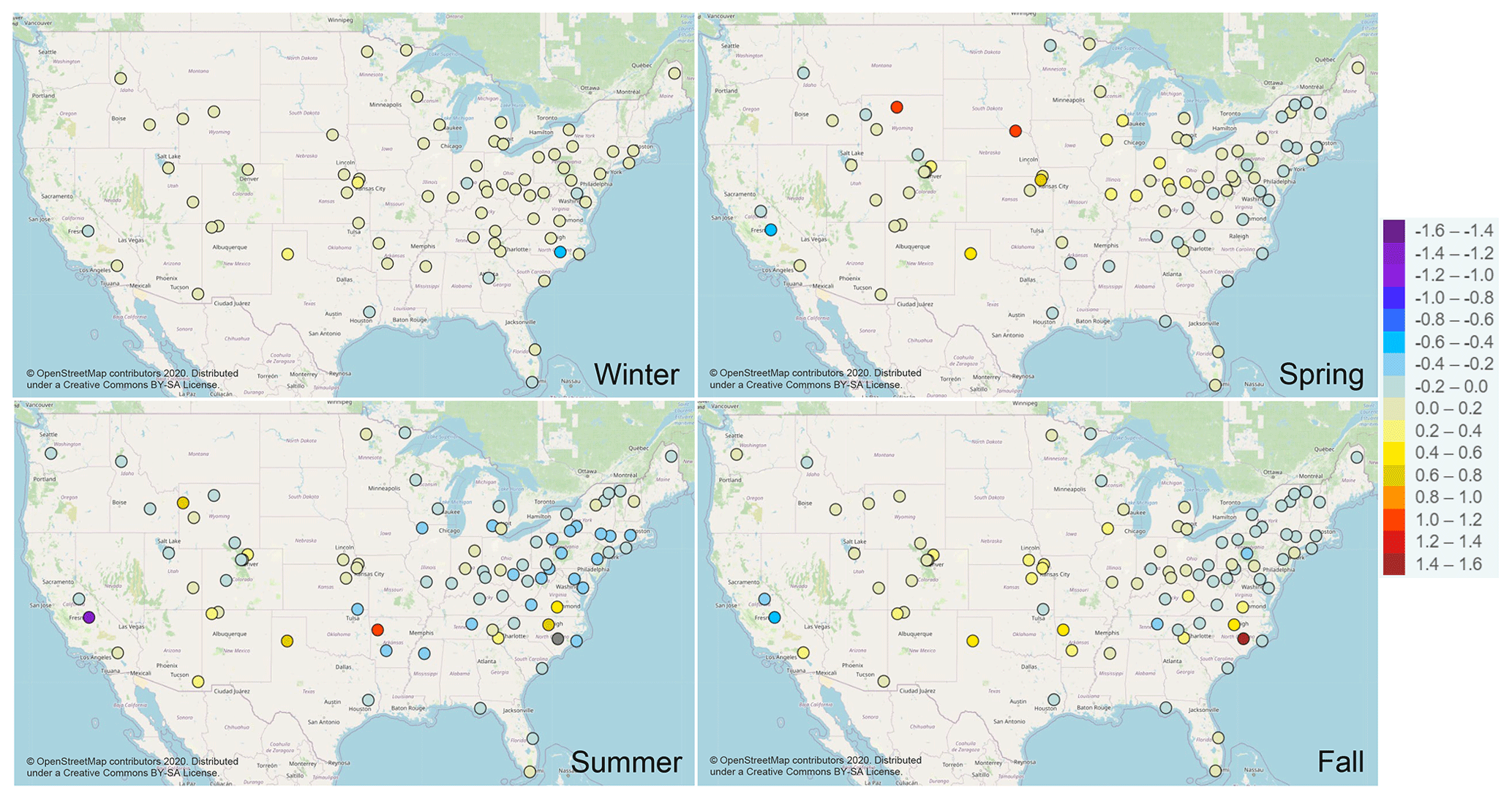
Figure 17Seasonal average NH3 absolute bias difference (µg m−3) between CMAQ531_WRF411_M3Dry_BiDi and CMAQ531_WRF411_STAGE_BiDi simulations for all AMON sites. Cool shading (negative values) indicates smaller bias in the CMAQ531_WRF411_M3Dry_BiDi simulation, and warm colors (positive values) indicate smaller bias in the CMAQ531_WRF411_STAGE_BiDi simulation. Grey shading indicates values beyond the range of the scale.
For ambient NH3, M3Dry and STAGE perform similarly throughout the year, with some notable exceptions. The time series in Fig. 16 shows the observed monthly average NH3 concentration from the AMON network sites, along with the corresponding simulated NH3 concentrations and monthly mean bias, RMSE, and Pearson correlation coefficient for the M3Dry and STAGE simulations. While both bidirectional models capture the overall trend in observed NH3, with lower concentrations in winter that peak in summer, both models underestimate the observed monthly average NH3 concentrations by 0.2–1.0 µg m−3. The STAGE model performs slightly better outside of summer, with lower bias and RMSE from January through May and October through November and higher correlation throughout the year. In summer, M3Dry has smaller bias, roughly half that of STAGE for July through September, but higher RMSE and lower correlation. The seasonal average NH3 spatial plots (Fig. 17) show little difference in absolute bias between M3Dry and STAGE in winter and relatively small differences in spring, except at two sites in the west that have significantly smaller (>1.0 µg m−3) bias with STAGE and one site in the central SJV of California that has smaller bias (0.5 µg m−3) with M3Dry. The difference in bias for the remaining sites is generally less than 0.1 µg m−3. In summer and fall, NH3 bias is lower (0.1–0.3 µg m−3) across most sites in the Northeast and Mid-Atlantic with M3Dry, while most sites west of the Mississippi River show a relatively small (<0.1 µg m−3) difference in bias between the two models. There are some notable exceptions, such as several sites in southern Virginia and North Carolina where STAGE has significantly smaller (0.5–2.0 µg m−3) bias, as well as sites in Arkansas, Texas, and Wyoming, while M3Dry maintains smaller bias for sites in the SJV of California and several sites in the Midwest.
CMAQ53 was publicly released in August 2019 and followed shortly by CMAQ531 in December 2019. The major science updates in the new model have been described, including extensive chemistry updates, the new AERO7 aerosol module, the updated M3Dry bidirectional deposition model, and the new STAGE bidirectional deposition model. Other significant updates to the CMAQ system include support for the HVC in WRF, updates to the PX-LSM and ACM2 PBL schemes in WRF and CMAQ, and the new DESID system. Evaluation of the science updates in CMAQ53 was accomplished by comparing monthly and seasonal MDA8 O3 and PM2.5 values from CMAQ531 simulations to a similarly configured CMAQ521 simulation for 2016. For MDA8 O3, CMAQ531 has consistently higher O3 in the winter versus CMAQ521, primarily due to reduced dry deposition to snow, and lower O3 throughout the rest of the year, particularly in spring, due primarily to reduced O3 in both the regional simulation and originating from the lateral BCs. The result is generally reduced MDA8 O3 bias in winter and summer and increased bias in spring and fall with CMAQ531. For PM2.5, CMAQ531 has lower concentrations on average in the spring and fall, higher concentrations in summer, and essentially unchanged concentrations in winter compared to CMAQ521. Overall for PM2.5, bias is slightly increased in spring and fall and slightly reduced in summer.
Comparisons were also made for the lateral BCs, meteorology model version, and the bidirectional surface exchange model to quantify their impacts on model results. Updating the source of lateral BCs from a HCMAQ521 simulation to a HCMAQ53 simulation increases O3 mixing ratios from the BCs in the northern latitudes (especially in winter and spring) due to the decreased O3 dry deposition to snow in CMAQ53, and reduces O3 mixing ratios in the middle and lower latitudes due to the updates to the bromine and iodine chemistry in CMAQ53, which reduces O3 mixing ratios over the ocean. Transitioning from WRF38 using the SVC to WRF411 using the HVC in the 12 km domain consistently increases (1.0–1.5 ppbv) MDA8 O3 mixing ratios throughout the year, while the impact on PM2.5 is smaller but also shows consistently higher concentrations (0.1–0.25 µg m−3) throughout the year. The differences in pollutant concentrations in CMAQ from using WRF38 and WRF411 are primarily attributed to differences in the treatment of VF and LAI in the LSM in the two versions of WRF. Using MODIS-derived vegetation parameters in WRF411 results in overall lower values of VF and LAI compared to the NLCD-derived values in WRF38, particularly in western North America. Finally, for the M3Dry and STAGE models, MDA8 O3 is similar in summer between the two models but generally higher with M3Dry outside of summer. For PM2.5, STAGE has consistently higher concentrations throughout the year, driven by differences in the assumptions affecting deposition velocity of particles in the two models. For ambient NH3, STAGE has slightly higher concentrations and a smaller bias in spring and fall, M3Dry has higher concentrations and a smaller bias in summer, and both models have relatively similar concentrations in winter. Model error tends to be lower and correlation tends to be higher for NH3 throughout the year with STAGE versus M3Dry.
While these versions of the CMAQ modeling system represent significant advancement in model process and input data science, several performance issues remain. The large underestimation of O3 in spring highlights the need for further improvement in representing the impacts of large-scale O3 distributions (e.g., international emissions, marine chemistry, stratosphere–troposphere exchange) and dry deposition across different surfaces that influence low- to mid-level O3 mixing ratios simulated by the model. Ozone continues to be underestimated in California throughout the year, a long-standing issue previously noted by Appel et al. (2017). The persistent underestimation is likely due to inaccurate representation of California emissions in the inventory used, as well as inability of the current 12 km resolution to capture atmospheric dynamics in the complex terrain in the region. CMAQ's performance in representing spatial and seasonal variations in ambient PM2.5 has improved considerably over the last decade as a result of improvements in representation of PM formation pathways and emissions, but CMAQ still tends to underestimate total PM2.5 mass in the southern and western US throughout much of the year, driven primarily by a large underestimation of PMother followed by a smaller underestimation of NO. Although efforts have been made to quantify the species that comprise the unidentified PM2.5 mass in the observations, more work is required to further improve the emission inventories for primary PM and consequently model performance.
The CMAQ version 5.3 (https://doi.org/10.5281/zenodo.3379043, United States Environmental Protection Agency, 2019a) and 5.3.1 (https://doi.org/10.5281/zenodo.3585898, United States Environmental Protection Agency, 2019b) codes and MCIP version 4.5 and 5.0 codes are available from the CMAQ GitHub site (https://github.com/USEPA/CMAQ, last access: 7 May 2021, Appel et al, 2017). The AMET code is available from the AMET GitHub site (https://github.com/USEPA/AMET, last access: 7 May 2021, Appel et al., 2011).
All data used in this work are available upon request from the authors. Please contact the corresponding author to request any data related to this work.
The supplement related to this article is available online at: https://doi.org/10.5194/gmd-14-2867-2021-supplement.
KWA led the development of this manuscript and was responsible for most of the model evaluation components presented in Sect. 4. JOB, KMF, RCG, WTH, DK, RM, BNM, SLN, CGN, JEP, GAP, HOTP, LR, SJR, GS, DBS, FS, TLS, and DCW contributed to the CMAQv5.3 code development and also contributed directly to the writing of Sect. 2 of this paper. Authors KMF and CH contributed to the writing of Sect. 3 and the model evaluation components of this study.
The authors declare that they have no conflict of interest.
The views expressed in this article are those of the authors and do not necessarily represent the views or policies of the U.S. Environmental Protection Agency.
Special thanks to Lara Reynolds with General Dynamics Information Technology, Inc (GDIT), for performing the WRF38 simulation used in this work. Special thanks to Liz Adams with the University of North Carolina (UNC) for her extensive testing of the CMAQ53 modeling system. Special thanks to Deborah Luecken, now retired from the EPA, for her significant contributions to the development of CMAQ53 and her decades of tireless work on the CMAQ modeling system. The authors would like to thank the two anonymous reviewers for their time and effort to review the manuscript and for their helpful suggestions that improved the final version of the paper.
This paper was edited by Samuel Remy and reviewed by two anonymous referees.
Appel, K. W., Gilliam, R. C., Davis, N., Zubrow, A., and Howard, S. C.: Overview of the Atmospheric Model Evaluation Tool (AMET) v1.1 for evaluating meteorological and air quality models, Environ. Modell. Softw., 26, 434–443, https://doi.org/10.1016/j.envsoft.2010.09.007, 2011.
Appel, K. W., Napelenok, S. L., Foley, K. M., Pye, H. O. T., Hogrefe, C., Luecken, D. J., Bash, J. O., Roselle, S. J., Pleim, J. E., Foroutan, H., Hutzell, W. T., Pouliot, G. A., Sarwar, G., Fahey, K. M., Gantt, B., Gilliam, R. C., Heath, N. K., Kang, D., Mathur, R., Schwede, D. B., Spero, T. L., Wong, D. C., and Young, J. O.: Description and evaluation of the Community Multiscale Air Quality (CMAQ) modeling system version 5.1, Geosci. Model Dev., 10, 1703–1732, https://doi.org/10.5194/gmd-10-1703-2017, 2017.
Bachmann, J. D.: Will the Circle Be Unbroken: A History of the U.S. National Ambient Air Quality Standards, J. Air Waste Manage., 57, 652–697, 2007.
Bash, J. O., Cooter, E. J., Dennis, R. L., Walker, J. T., and Pleim, J. E.: Evaluation of a regional air-quality model with bidirectional NH3 exchange coupled to an agroecosystem model, Biogeosciences, 10, 1635–1645, https://doi.org/10.5194/bg-10-1635-2013, 2013.
Byun, D. and Schere, K. L.: Review of the governing equations, computational algorithms, and other components of the Models-3 Community Multiscale Air Quality (CMAQ) modeling system, Appl. Mech. Rev., 59, 51–77, 2006.
Carlton, A. G., Bhave, P. V., Napelenok, S. L., Edney, E. O., Sarwar, G., Pinder, R. W., Pouliot, G. A., and Houyoux, M.: Model Representation of Secondary Organic Aerosol in CMAQv4.7, Environ. Sci. Technol. 44, 8553–8560, https://doi.org/10.1021/es100636q, 2010.
Damian, V., Sandu, A., Damian, M., Potra, F., and Carmichael, G. R.: The Kinetic PreProcessor KPP – A software environment for solving chemical kinetics, Comput. Chem. Eng., 26, 1567–1579, 2002.
Dennis, R., Fox, T., Fuentes, M., Gilliland, A., Hanna, S., Hogrefe, C., Irwin, J., Rao, S. T., Scheffe, R., Schere, K., Steyn, D., and Venkatram, A.: A framework for evaluating regional-scale numerical photochemical modeling system, Environ. Fluid Mech., 10, 471–489, https://doi.org/10.1007/s10652-009-9163-2, 2010.
Fahey, K. M. and Roselle, S.: Investigating aqueous production pathways of particulate sulfur in CMAQ with AQCHEM-KMT (version 2) and the sulfur tracking method, in: 18th Annual CMAS Conference, Chapel Hill, North Carolina, USA, 2019.
Fahey, K. M., Carlton, A. G., Pye, H. O. T., Baek, J., Hutzell, W. T., Stanier, C. O., Baker, K. R., Appel, K. W., Jaoui, M., and Offenberg, J. H.: A framework for expanding aqueous chemistry in the Community Multiscale Air Quality (CMAQ) model version 5.1, Geosci. Model Dev., 10, 1587–1605, https://doi.org/10.5194/gmd-10-1587-2017, 2017a.
Fahey, K. M., Sareen, N., Carlton, A. G., Hutzell, W. T., and Luecken, D. J.: Regional impacts of extending inorganic and organic cloud chemistry with AQCHEM-KMT, in: 16th Annual CMAS Conference, Chapel Hill, North Carolina, USA, poster no. 17, 2017b.
Fares, S., Weber, R., Park, J.-H., Gentner, D., Karlik, J., and Goldstein, A. H.: Ozone deposition to an orange orchard: partitioning between stomatal and non-stomatal sinks, Environ. Pollut., 169, 258–266, https://doi.org/10.1016/j.envpol.2012.01.030, 2012.
Fares, S., Savi, F., Muller, J., Matteucci, G., and Paoletti, E.: Simultaneous measurements of above and below canopy ozone fluxes help partitioning ozone deposition between its various sinks in a Mediterranean Oak Forest, Agr. Forest Meteorol., 198–199, 181–191, https://doi.org/10.1016/j.agrformet.2014.08.014, 2014.
Fry, J. L., Draper, D. C., Barsanti, K. C., Smith, J. N., Ortega, J., Winkler, P. M., Lawler, M. J., Brown, S. S., Edwards, P. M., Cohan, R. C., and Lee, L.: Secondary Organic Aerosol Formation and Organic Nitrate Yield from NO3 Oxidation of Biogenic Hydrocarbons, Environ. Sci. Technol., 48, 11944–11953, https://doi.org/10.1021/es502204x, 2014.
Fumagalli, I., Gruening, C., Marzouli, R., Cieslik, S., and Gerosa, G.: Long-term measurements of NOx and O3 soil fluxes in a temperate deciduous forest, Agr. Forest Meteorol., 228–229, 205–216, https://doi.org/10.1016/j.agrformet.2016.07.011, 2016.
Giorgi, F.: A particle dry-deposition parameterization scheme for use in tracer transport models, J. Geophys. Res.-Atmos., 91, 9794–9806, https://doi.org/10.1029/JD091iD09p09794, 1986.
Guenther, A. B., Jiang, X., Heald, C. L., Sakulyanontvittaya, T., Duhl, T., Emmons, L. K., and Wang, X.: The Model of Emissions of Gases and Aerosols from Nature version 2.1 (MEGAN2.1): an extended and updated framework for modeling biogenic emissions, Geosci. Model Dev., 5, 1471–1492, https://doi.org/10.5194/gmd-5-1471-2012, 2012.
Heath, N., Pleim, J., Gilliam, R., and Kang, D.: A simple lightning assimilation technique for improving retrospective WRF simulations, J. Adv. Model. Earth Sy., 8, 1806–1824, https://doi.org/10.1002/2016MS000735, 2016.
Helmig, D., Ganzeveld, L., Butler, T., and Oltmans, S. J.: The role of ozone atmosphere-snow gas exchange on polar, boundary-layer tropospheric ozone – a review and sensitivity analysis, Atmos. Chem. Phys., 7, 15–30, https://doi.org/10.5194/acp-7-15-2007, 2007.
Hogrefe, C., Liu, P., Pouliot, G., Mathur, R., Roselle, S., Flemming, J., Lin, M., and Park, R. J.: Impacts of different characterizations of large-scale background on simulated regional-scale ozone over the continental United States, Atmos. Chem. Phys., 18, 3839–3864, https://doi.org/10.5194/acp-18-3839-2018, 2018.
Iacono, M. J., Delamere, J. S., Mlawer, E. J., Shephard, M. W., Clough, S. A., and Collins, W.: Radiative forcing by long-lived greenhouse gases: Calculations with the AER radiative transfer models, J. Geophys. Res.-Atmos., 113, D13103, https://doi.org/10.1029/2008JD009944, 2008.
Janssens-Maenhout, G., Crippa, M., Guizzardi, D., Dentener, F., Muntean, M., Pouliot, G., Keating, T., Zhang, Q., Kurokawa, J., Wankmüller, R., Denier van der Gon, H., Kuenen, J. J. P., Klimont, Z., Frost, G., Darras, S., Koffi, B., and Li, M.: HTAP_v2.2: a mosaic of regional and global emission grid maps for 2008 and 2010 to study hemispheric transport of air pollution, Atmos. Chem. Phys., 15, 11411–11432, https://doi.org/10.5194/acp-15-11411-2015, 2015.
Kain, J. S.: The Kain-Fritsch convective parameterization: An update, J. Appl. Meteorol., 43, 170–181, https://doi.org/10.1175/1520-0450(2004)043<0170:TKCPAU>2.0.CO;2, 2004.
Kang, D., Foley, K. M., Mathur, R., Roselle, S. J., Pickering, K. E., and Allen, D. J.: Simulating lightning NO production in CMAQv5.2: performance evaluations, Geosci. Model Dev., 12, 4409–4424, https://doi.org/10.5194/gmd-12-4409-2019, 2019a.
Kang, D., Pickering, K. E., Allen, D. J., Foley, K. M., Wong, D. C., Mathur, R., and Roselle, S. J.: Simulating lightning NO production in CMAQv5.2: evolution of scientific updates, Geosci. Model Dev., 12, 3071–3083, https://doi.org/10.5194/gmd-12-3071-2019, 2019b.
Kelly, J. T., Koplitz, S. N., Baker, K. R., Holder, A. L., Pye, H. O. T., Murphy, B. N., Bash, J. O., Henderson, B. H., Possiel, N. C., Simon, H., Eyth, A. M., Jang, C., Phillips, S., and Timin, B.: Assessing PM2.5 model performance for the conterminous U.S. with comparison to model performance statistics from 2007–2015, Atmos. Environ., 214, https://doi.org/10.1016/j.atmosenv.2019.116872, 2019.
Kondo, J., Saigusa, N., and Sato, T.: A parameterization of evaporation from bare soils surfaces, J. App. Meteorol. Clim. 29, 385–389, https://doi.org/10.1175/1520-0450(1990)029<0385:APOEFB>2.0.CO;2, 1990.
Kwok, R. H. F., Napelenok, S. L., and Baker, K. R.: Implementation and evaluation of PM2.5 source contribution analysis in a photochemical model, Atmos. Environ., 80, 398–407, https://doi.org/10.1016/j.atmosenv.2013.08.017, 2013.
Kwok, R. H. F., Baker, K. R., Napelenok, S. L., and Tonnesen, G. S.: Photochemical grid model implementation and application of VOC, NOx, and O3 source apportionment, Geosci. Model Dev., 8, 99–114, https://doi.org/10.5194/gmd-8-99-2015, 2015.
Leriche, M., Pinty, J.-P., Mari, C., and Gazen, D.: A cloud chemistry module for the 3-D cloud-resolving mesoscale model Meso-NH with application to idealized cases, Geosci. Model Dev., 6, 1275–1298, https://doi.org/10.5194/gmd-6-1275-2013, 2013.
Lim, H.-J., Carlton, A. G., and Turpin, B. J.: Isoprene forms secondary organic aerosol through cloud processing: model simulations, Environ. Sci. Technol., 39, 4441–4446, https://doi.org/10.1021/es048039h, 2005.
Lim, Y. B., Tan, Y., Perri, M. J., Seitzinger, S. P., and Turpin, B. J.: Aqueous chemistry and its role in secondary organic aerosol (SOA) formation, Atmos. Chem. Phys., 10, 10521–10539, https://doi.org/10.5194/acp-10-10521-2010, 2010.
Lim, Y. B., Tan, Y., and Turpin, B. J.: Chemical insights, explicit chemistry, and yields of secondary organic aerosol from OH radical oxidation of methylglyoxal and glyoxal in the aqueous phase, Atmos. Chem. Phys., 13, 8651–8667, https://doi.org/10.5194/acp-13-8651-2013, 2013.
Luecken, D. J., Yarwood, G., and Hutzell, W. T.: Multipollutant modeling of ozone, reactive nitrogen and HAPs across the continental US with CMAQ-CB6, Atmos. Environ., 201, 62–72, https://doi.org/10.1016/j.atmosenv.2018.11.060, 2019.
Massad, R.-S., Nemitz, E., and Sutton, M. A.: Review and parameterisation of bi-directional ammonia exchange between vegetation and the atmosphere, Atmos. Chem. Phys., 10, 10359–10386, https://doi.org/10.5194/acp-10-10359-2010, 2010.
Mathur, R., Xing, J., Gilliam, R., Sarwar, G., Hogrefe, C., Pleim, J., Pouliot, G., Roselle, S., Spero, T. L., Wong, D. C., and Young, J.: Extending the Community Multiscale Air Quality (CMAQ) modeling system to hemispheric scales: overview of process considerations and initial applications, Atmos. Chem. Phys., 17, 12449–12474, https://doi.org/10.5194/acp-17-12449-2017, 2017.
Mesinger, F., DiMego, G., Kalnay, E., Mitchell, K., Shafran, P. C., Ebisuzaki, W., Jović, D., Woollen, J., Rogers, E., Berbery, E. H., Ek, M. B., Fan, Y., Grumbine, R., Higgins, W., Li, H., Lin, Y., Manikin, G., Parrish, D., and Shi, W.: North American Regional Reanalysis, B. Am. Meteorol. Soc., 87, 343–360, https://doi.org/10.1175/BAMS-87-3-343, 2006.
Mészáros, R., Horváth, L., Weidinger, T., Neftel, A., Nemitz, E., Dämmgen, U., Cellier, P., and Loubet, B.: Measurement and modelling ozone fluxes over a cut and fertilized grassland, Biogeosciences, 6, 1987–1999, https://doi.org/10.5194/bg-6-1987-2009, 2009.
Morrison, H., Curry, J. A., and Khvorostyanov, V. I.: A new doublemoment microphysics parameterization for application in cloud and climate models, Part I: Description, J. Atmos. Sci., 62, 1665–1677, https://doi.org/10.1175/JAS3446.1, 2005.
Murphy, B. N., Woody, M. C., Jimenez, J. L., Carlton, A. M. G., Hayes, P. L., Liu, S., Ng, N. L., Russell, L. M., Setyan, A., Xu, L., Young, J., Zaveri, R. A., Zhang, Q., and Pye, H. O. T.: Semivolatile POA and parameterized total combustion SOA in CMAQv5.2: impacts on source strength and partitioning, Atmos. Chem. Phys., 17, 11107–11133, https://doi.org/10.5194/acp-17-11107-2017, 2017.
Murphy, B. N., Nolte, C. G., Sidi, F., Bash, J. O., Appel, K. W., Jang, C., Kang, D., Kelly, J., Mathur, R., Napelenok, S., Pouliot, G., and Pye, H. O. T.: The Detailed Emissions Scaling, Isolation, and Diagnostic (DESID) module in the Community Multiscale Air Quality (CMAQ) Modeling System version 5.3, Geosci. Model Dev. Discuss. [preprint], https://doi.org/10.5194/gmd-2020-361, in review, 2020.
Nemitz, E., Milford, C., and Sutton, M. A.: A two-layer canopy compensation point model for describing bi-directional biosphere-atmosphere exchange of ammonia, Q. J. Roy. Meteor. Soc., 127, 815–833, https://doi.org/10.1002/qj.49712757306, 2001.
Noilhan, J. and Mahfouf, J. F.: The ISBA land surface parameterization scheme, Global Planet. Change, 13, 145–159, https://doi.org/10.1016/0921-8181(95)00043-7, 1996.
Otte, T. L. and Pleim, J. E.: The Meteorology-Chemistry Interface Processor (MCIP) for the CMAQ modeling system: updates through MCIPv3.4.1, Geosci. Model Dev., 3, 243–256, https://doi.org/10.5194/gmd-3-243-2010, 2010.
Pleim, J. E.: A simple, efficient solution of flux-profile relationships in the atmospheric surface layer, J. Appl. Meteorol. Clim., 45, 341–347, https://doi.org/10.1175/JAM2339.1, 2006.
Pleim, J. E.: A combined local and nonlocal closure model for the atmospheric boundary layer, Part I: model description and testing, J. Appl. Meteorol. Clim., 46, 1383–1395, https://doi.org/10.1175/JAM2539.1, 2007a.
Pleim, J. E.: A combined local and nonlocal closure model for the atmospheric boundary layer, Part II: application and evaluation in a mesoscale meteorological model, J. Appl. Meteorol. Clim., 46, 1396–1409, https://doi.org/10.1175/JAM2534.1, 2007b.
Pleim, J. E. and Gilliam, R. C.: An indirect data assimilation scheme for deep soil temperature in the Pleim-Xiu land surface model, J. Appl. Meteorol. Clim., 48, 1362–1376, https://doi.org/10.1175/2009JAMC2053.1, 2009.
Pleim, J. E., Bash, J. O., Walker, J. T., and Cooter, E. J.: Development and testing of an ammonia bi-directional flux model for air-quality models, J. Geophys. Res.-Atmos., 118, 3794–3806, https://doi.org/10.1002/jgrd.50262, 2013.
Pleim, J. E., Ran, L., Appel, W., Shephard, M. W., and Cady-Pereira, K.: New bidirectional ammonia flux model in an air quality model coupled with an agricultural model, J. Adv. Model. Earth Sy., 11, 2934–2957, https://doi.org/10.1029/2019MS001728, 2019.
Pye, H. O. T., Chan, A. W. H., Barkley, M. P., and Seinfeld, J. H.: Global modeling of organic aerosol: the importance of reactive nitrogen (NOx and NO3), Atmos. Chem. Phys., 10, 11261–11276, https://doi.org/10.5194/acp-10-11261-2010, 2010.
Pye, H. O. T., Pinder, R. W., Piletic, I., Xie, Y., Capps, S. L., Lin, Y.-H., Surratt, J. D., Zhang, Z., Gold, A., Luecken, D. J., Hutzell, W. T., Jaoui, M., Offenberg, J. H., Kleindienst, T. E., Lewandowski, M., and Edney, E. O.: Epoxide pathways improve model predictions of isoprene markers and reveal key role of acidity in aerosol formation, Environ. Sci. Technol., 47, 11056–11064, https://doi.org/10.1021/es402106h, 2013.
Pye, H. O. T., Luecken, D. J., Xu, L., Boyd, C. M., Ng, N. L., Baker, K., Ayres, B. A., Bash, J. O., Baumann, K., Carter, W. P. L., Edgerton, E., Fry, J. L., Hutzell, W. T., Schwede, D., and Shepson, P. B.: Modeling the current and future roles of particulate organic nitrates in the southeastern United States, Environ. Sci. Technol., 49, 14195–14203, https://doi.org/10.1021/acs.est.5b03738, 2015.
Pye, H. O. T., Murphy, B. N., Xu, L., Ng, N. L., Carlton, A. G., Guo, H., Weber, R., Vasilakos, P., Appel, K. W., Budisulistiorini, S. H., Surratt, J. D., Nenes, A., Hu, W., Jimenez, J. L., Isaacman-VanWertz, G., Misztal, P. K., and Goldstein, A. H.: On the implications of aerosol liquid water and phase separation for organic aerosol mass, Atmos. Chem. Phys., 17, 343–369, https://doi.org/10.5194/acp-17-343-2017, 2017.
Pye, H. O. T., D'Ambro, E. L., Lee, B. H., Schobesberger, S., Takeuchi, M., Zhao, Y., Lopez-Hilfiker, F., Liu, J., Shilling, J. E., Xing, J., Mathur, R., Middlebrook, A. M., Liao, J., Welti, A., Graus, M., Warneke, C., de Gouw, J. A., Holloway, J. S., Ryerson, T. B., Pollack, I. B., and Thornton, J. A.: Anthropogenic enhancements to production of highly oxygenated molecules from autoxidation, P. Natl. Acad. Sci. USA, 116, 6641–6646, https://doi.org/10.1073/pnas.1810774116, 2019.
Qin, M., Murphy, B. N., Isaacs, K. K., McDonald, B. C., Lu, Q., McKeen, S. A., Koval, L., Robinson, A. L., Efstathious, C., Allen, C., and Pye, H. O. T.: Criteria pollutant impacts of volatile chemical products informed by near-field modeling, Nat Sustain, 4, 129–137, https://doi.org/10.1038/s41893-020-00614-1, 2021.
Ran, L., Gilliam, R., Binkowski, F. S., Xiu, A., Pleim, J., and Band, L.: Sensitivity of the Weather Research and Forecast/Community Multiscale Air Quality modeling system to MODIS LAI, FPAR, and albedo, J. Geophys. Res.-Atmos., 120, 8491–8511, https://doi.org/10.1002/2015JD023424, 2015.
Ran, L., Pleim, J., Gilliam, R., Binkowski, F., Hogrefe, C., and Band, L.: Improved meteorology from an updated WRF/CMAQ modeling system with MODIS vegetation and albedo, J. Geophys. Res.-Atmos., 121, 2393–2415, https://doi.org/10.1002/2015JD024406, 2016.
Ran, L., Yuan, Y., Cooter, E., Benson, V., Yang, D., Pleim, J., Wang, R., and Williams, J.: An integrated agriculture, atmosphere, and hydrology modeling system for ecosystem assessments, J. Adv. Model. Earth Sy., 11, 4645–4668, https://doi.org/10.1029/2019MS001708, 2019.
Saha, P. K. and Grieshop, A. P.: Exploring Divergent Volatility Properties from Yield and Thermodenuder Measurements of Secondary Organic Aerosol from α-Pinene Ozonolysis, Environ. Sci. Technol., 50, 5740–5749, https://doi.org/10.1021/acs.est.6b00303, 2016.
Sareen, N., Fahey, K., Hutzell, W., and Carlton, A. G.: Implementing explicit secondary organic aerosol (SOA) aqueous chemistry in CMAQ, in: 12th Annual CMAS Conference, 5–7 October 2013,, Chapel Hill, North Carolina, USA, available at: https://www.cmascenter.org/conference/2013/agenda.cfm#inline1286 (last access: 7 May 2021), 2013.
Sarwar, G., Fahey, K., Napelenok, S., Roselle, S., and Mathur, R.: Examining the impact of CMAQ model updates on aerosol sulfate predictions, in: The 10th Annual CMAS Models-3 User's Conference, 24–26 October 2011, Chapel Hill, North Carolina, USA, poster no. 28, available at: https://www.cmascenter.org/conference//2011/slides/sarwar_examining_impact_2011.pdf (last access: 7 May 2021), 2011.
Sarwar, G., Gantt, B., Schwede, D., Foley, K., Mathur, R., and Saiz-Lopez, A.: Impact of Enhanced Ozone Deposition and Halogen Chemistry on Tropospheric Ozone over the Northern Hemisphere, Environ. Sci. Technol., 49, 9203–9211, https://doi.org/10.1021/acs.est.5b01657, 2015.
Sarwar, G., Gantt, B., Foley, K., Fahey, K., Spero, T. L., Kang, D., Mathur, R., Foroutan, H., Xing, J., Sherwen, T., and Saiz-Lopez, A.: Influence of bromine and iodine chemistry on annual, seasonal, diurnal, and background ozone: CMAQ simulations over the Northern Hemisphere, Atmos. Environ., 213, 395–404, https://doi.org/10.1016/j.atmosenv.2019.06.020, 2019.
Schreiber, L. and Schoenherr, J.: Water and solute permeabilities of plant cuticles: measurements and data analysis, Springer, 299 pp., https://doi.org/10.1007/978-3-540-68945-4, 2009.
Schwartz, S. E.: Mass-transport considerations pertinent to aqueous-phase reactions of gases in liquid-water clouds, in: Chemistry of Multiphase Atmospheric Systems, NATO ASI Series, edited by: Jaescheke, W., Springer, Berlin, Heidelberg, 6, 415–471, https://doi.org/10.1007/978-3-642-70627-1_16, 1986.
Skamarock, W. C. and Klemp, J. B.: A time-split nonhydrostatic atmospheric model for weather research and forecasting applications, J. Comput. Phys., 227, 3465–3485, https://doi.org/10.1016/j.jcp.2007.01.037, 2008.
Slinn, W. G. N.: Predictions for particle deposition to vegetative canopies, Atmos. Environ., 16, 1785–1794, https://doi.org/10.1016/0004-6981(82)90271-2, 1982.
Swall, J. and Foley, K. M.: The impact of spatial correlation and incommensurability on model evaluation, Atmos. Environ., 43, 1204–1217, https://doi.org/10.1016/j.atmosenv.2008.10.057, 2009.
Swenson, S. C. and Lawrence, D. M.: Assessing a dry surface layer-based soil resistance parameterization for the Community Land-Model using GRACE and FLUXNET-MTE data, J. Geophys. Res.-Atmos., 119, 10299–10312, https://doi.org/10.1002/2014JD022314, 2014.
United States Environmental Protection Agency: CMAQ (Version 5.2.1) [Software], Zenodo, https://doi.org/10.5281/zenodo.1212601, 2018.
United States Environmental Protection Agency: CMAQ (Version 5.3) [Software], Zenodo, https://doi.org/10.5281/zenodo.3379043, 2019a.
United States Environmental Protection Agency: CMAQ (Version 5.3.1) [Software], Zenodo, https://doi.org/10.5281/zenodo.3585898, 2019b.
USEPA – U.S. Environmental Protection Agency: Development and Testing of a Dry Deposition Algorithm (Revised), EPA-454/R-94-015, PB94183100, U.S. Environmental Protection Agency, Office of Air Quality Planning and Standards, Washington, D.C., 1994.
Vukovich, J., Eyth, A., Henderson, B., Jang, C., Allen, C., Beidler, J., and Talgo, K.: Development of 2016 hemispheric emissions for CMAQ, in: 17th Annual CMAS Conference, 22–24 October 2018, Chapel Hill, North Carolina, USA, available at: https://www.cmascenter.org/conference//2018/slides/1530_vukovich_development_2016_2018.pptx (last access: 3 May 2021), 2018.
Wiedinmyer, C., Akagi, S. K., Yokelson, R. J., Emmons, L. K., Al-Saadi, J. A., Orlando, J. J., and Soja, A. J.: The Fire INventory from NCAR (FINN): a high resolution global model to estimate the emissions from open burning, Geosci. Model Dev., 4, 625–641, https://doi.org/10.5194/gmd-4-625-2011, 2011.
Williams J. R.: The EPIC model, in: Computer models of watershed hydrology, Water Resources Publications, Highlands Ranch, Colorado, USA, 909–1000, 1995.
Wu, Z., Schwede, D. B., Vet, R., Walker, J. T., Shaw, M., Staebler, R., and Zhang, L.: Evaluation and intercomparison of five North American dry deposition algorithms at a mixed forest site, J. Adv. Model. Earth Sy., 10, 1571–1586, https://doi.org/10.1029/2017MS001231, 2018.
Xing, J., Mathur, R., Pleim, J., Hogrefe, C., Wang, J., Gan, C.-M., Sarwar, G., Wong, D. C., and McKeen, S.: Representing the effects of stratosphere–troposphere exchange on 3-D O3 distributions in chemistry transport models using a potential vorticity-based parameterization, Atmos. Chem. Phys., 16, 10865–10877, https://doi.org/10.5194/acp-16-10865-2016, 2016.
Xu, L., Pye, H. O. T., He, J., Chen, Y., Murphy, B. N., and Ng, N. L.: Experimental and model estimates of the contributions from biogenic monoterpenes and sesquiterpenes to secondary organic aerosol in the southeastern United States, Atmos. Chem. Phys., 18, 12613–12637, https://doi.org/10.5194/acp-18-12613-2018, 2018.
Yarwood, Y., Sakulyanontvittaya, T., Nopmongcol, O., and Koo, K.: Ozone depletion by bromine and iodine over the Gulf of Mexico, final report for the Texas Commission on Environmental Quality, available at: https://www.tceq.texas.gov/assets/public/implementation/air/am/contracts/reports/pm/5821110365FY1412-20141109-environ-bromine.pdf (last access: 3 May 2021), November 2014.
Yi, C.: Momentum transfer within canopies, J. Appl. Meteorol. Clim., 47, 262–275, https://doi.org/10.1175/2007JAMC1667.1, 2008.
Zhang, H., Yee, L. D., Lee, B. H., Curtis, M. P., Worton, D. R., Isaacman-VanWertz, G., Offenberg, J. H., Lewandowski, M., Kleindienst, T. E., Beaver, M. R., Holder, A. L., Lonneman, W. A., Docherty, K. S., Jaoui, M., Pye, H. O. T., Hu, W., Day, D. A., Campuzano-Jost, P., Jimenez, J. L., Guo, H., Weber, R. J., de Gouw, J., Koss, A. R., Edgerton, E. S., Brune, W., Mohr, C., Lopez-Hilfiker, F. D., Lutz, A., Kreisberg, N. M., Spielman, S. R., Hering, S. V., Wilson, K. R., Thornton, J. A., and Goldstein, A. H.: Monoterpenes are the largest source of summertime organic aerosol in the southeastern United States, P. Natl. Acad. Sci. USA, 115, 2038–2043, https://doi.org/10.1073/pnas.1717513115, 2018.
Zhang, L., Gong, S., Padro, J., and Barrie, L.: A size-segregated particle dry deposition scheme for an atmospheric aerosol module, Atmos. Environ., 35, 549–560, https://doi.org/10.1016/S1352-2310(00)00326-5, 2001.
Zhao, J., Sarwar, G., Brett, G., Foley, K., Henderson, B. H., Pye, H. O. T., Fahey, K., Kang, D., Mathur, R., Zhang, Y., Li, Q., and Saiz-Lopez, A.: Impact of dimethylsulfide chemistry on air quality over the Northern Hemisphere, Atmos. Environ., 244, 117961, https://doi.org/10.1016/j.atmosenv.2020.117961, 2021.