the Creative Commons Attribution 4.0 License.
the Creative Commons Attribution 4.0 License.
 | 20 May 2021
TransEBM v. 1.0: description, tuning, and validation of a transient model of the Earth's energy balance in two dimensions
Elisa Ziegler
Kira Rehfeld
Modeling the long-term transient evolution of climate remains a technical and scientific challenge. However, understanding and improving modeling of the long-term behavior of the climate system increases confidence in projected changes in the mid- to long-term future. Energy balance models (EBMs) provide simplified and computationally efficient descriptions of long timescales and allow large ensemble runs by parameterizing energy fluxes. In this way, they can be used to pinpoint periods and phenomena of interest. Here, we present TransEBM, an extended version of the two-dimensional energy balance model by Zhuang et al. (2017a). Transient CO2, solar insolation, orbital configuration, fixed ice coverage, and land–sea distribution are implemented as effective radiative forcings at the land surface. We show that the model is most sensitive to changes in CO2 and ice distribution, but the obliquity and land–sea mask have significant influence on modeled temperatures as well. We tune TransEBM to reproduce the 1960–1989 CE global mean temperature and the Equator-to-pole and seasonal temperature gradients of ERA-20CM reanalysis (Hersbach et al., 2015). The resulting latitudinal and seasonal temperature distributions agree well with reanalysis and the general circulation model (GCM) HadCM3 for a simulation of the past millennium (Bühler et al., 2020). TransEBM does not represent the internal variability of the ocean–atmosphere system, but non-deterministic elements and nonlinearity can be introduced through model restarts and randomized forcing. As the model facilitates long transient simulations, we envisage its use in exploratory studies of stochastic forcing and perturbed parameterizations, thus complementing studies with comprehensive GCMs.
- Article
(7908 KB) - Full-text XML
- BibTeX
- EndNote


Observational records of climate and proxies are limited in both time and space (Schmidt et al., 2014; Hersbach et al., 2015). As such, climate models are vital for climate research since they can fill in gaps left by observational records. Such gaps exist both during the instrumental era and in paleoclimate, e.g., with respect to transitions and hysteresis in climate (e.g., Rahmstorf et al., 2005; Abe-Ouchi et al., 2013; Ghil, 2015; Fraedrich et al., 2016; Stap et al., 2017) or variability in the climate system (Huybers and Curry, 2006; Laepple and Huybers, 2014; Rehfeld et al., 2020). They allow for the study of questions about past changes in climate like the Holocene temperature conundrum (Liu et al., 2014) or the response to changes in boundary conditions, thus improving the understanding of the past, present, and future states of the climate system (Braconnot et al., 2012; Schmidt et al., 2014). To provide confidence regarding their results, large ensembles are necessary (Collins et al., 2013; Schmidt et al., 2014). However, due to constraints in computational resources, to date state-of-the-art Earth system or general circulation models (GCMs) can only offer transient simulations for limited timescales (Smith and Gregory, 2012; Liu et al., 2009; Stap et al., 2017; Otto-Bliesner et al., 2017) unless they restrict the complexity of the models (e.g., Goosse et al., 2010; Smith and Gregory, 2012; Andres and Tarasov, 2019; Stap et al., 2018). Long timescales in particular have been simulated by taking snapshots of equilibrium states instead (e.g., Singarayer and Valdes, 2010). In this context, low-complexity models such as energy balance models (EBMs) are viable alternatives since their computational efficiency allows the running of fast and repeated simulations.
EBMs compute the temperature field based on the difference between incoming solar and outgoing terrestrial radiation. Unlike GCMs, EBMs do not contain parameterizations of the whole climate system and instead focus on the Earth's energy balance and parameterization of energy fluxes. They were among the first climate models developed and helped build the current understanding of the climate system (North and Kim, 2017). However, many of the early studies cannot be reproduced today, since the models were not preserved (Zhuang et al., 2017a). This motivated Zhuang et al. (2017a) to publish their model code for a two-dimensional EBM, which serves as the basis of this study.
Arrhenius (1896) was the first to estimate the Earth's energy balance in order to calculate its global mean temperature response to the influence of greenhouse gases. In the late 1960s, Budyko (1968) and Sellers (1969) introduced EBMs as one-dimensional models with latitudinal energy transport and investigated their response to changes in solar radiation. Sellers (1969) contributed an early study on the effect of human greenhouse gas emissions. North and Coakley (1979) added a seasonal cycle and later introduced a longitudinal dimension (North et al., 1980, 1983) so that their EBM could simulate a two-dimensional representation of global temperatures.
North et al. (1983) incorporated seasonality in the two-dimensional EBM and investigated the lag of the annual cycle with respect to solar forcing and how seasonality interacts with changes in orbital parameters. They showed how configurations of orbital parameters can lead to colder seasons in the Northern Hemisphere that favor glaciation. Others studied seasonality under varying continental configurations throughout Earth's history (Crowley et al., 1986; Mengel et al., 1988; Crowley et al., 1989; Hyde et al., 1989; Short et al., 1991). For example, examining the effect of changing land–sea distributions on the seasonal cycle, Crowley et al. (1986) and Crowley et al. (1989) found considerable differences in summer temperatures throughout the ages depending on land–sea distribution. Huang and Bowman (1992) conducted a similar study, focusing on the seasonal snowline instability and the response of the ice albedo feedback to variations in land–sea distribution and seasonality.
Many of these studies examined seasonality in conjunction with not just the snowline instability but the whole cryosphere, whose influence on Earth's climate has long been of interest. Sellers (1969) had already examined the idea of an ice-free Arctic in response to continued and increasing greenhouse gas emissions, and numerous studies followed that investigated the small ice cap instability and its relation to the formation of the Antarctic ice sheet (North et al., 1983; North, 1984; Mengel et al., 1988; Crowley and North, 1990; Huang and Bowman, 1992). To examine the small ice cap instability, they simulated whether snow and ice accumulates or melts based on midsummer temperatures. The albedo field was then changed in accordance with the simulated snowline. In this way, these studies were able to simulate the response of the ice cover to changes in solar insolation or greenhouse gas concentration.
Crowley and North (1990) additionally analyzed transitions into glacial states. In fact, several of the studies found abrupt transitions and hysteresis in the creation and disappearance of ice sheets (North et al., 1983; Mengel et al., 1988; Crowley and North, 1990; Zhuang et al., 2014), as well as the possibility of multiple stable states with and without ice co-existing (North et al., 1983; North, 1984; Mengel et al., 1988). These studies built on both Budyko (1968) and Sellers (1969), who already demonstrated that EBMs can be used to study hysteresis in the climate system. They found that changes in solar radiation might lead to transitions between stable states and discussed under which conditions an ice-covered Earth could be possible. All of these studies suggest that there are multiple stable states in the climate system that climate can transition between.
Crowley and North (1988) and Crowley and Hyde (2008) relate such transitions to increasing variability in the climate system. They argue that an increase in variability indicates a predisposition of Earth's climate towards tipping into a different state in response to small changes in boundary conditions. Ghil (2015) investigated climate variability and sensitivity from a system dynamics standpoint to understand variability on all timescales. For this, the study used zero- to two-dimensional EBMs as part of a model hierarchy to show how multiple equilibria arise and how internal variability interacts with forcings. Dortmans et al. (2019) also found evidence for bifurcations and possible transitions between stable states in relation to glaciation. They connected these transitions to particular points in the geological past using a zero-dimensional EBM. At these points, they investigated possible mechanisms that explain sudden glaciations or unusually warm periods, focusing mainly on CO2, water vapor, and oceanic and atmospheric heat transport. Overall, EBMs are able to simulate hysteresis and tipping points, whereas CMIP5 GCMs struggle to simulate such strong transitions, as shown for Arctic sea ice (Wagner and Eisenman, 2015; Bathiany et al., 2016), as well as the Atlantic meridional overturning circulation and other proposed tipping points (Bathiany et al., 2016).
Further studies of Earth's climatic history include the simulation of a possible climate on the supercontinent Pangaea during the early Late Permian (Crowley et al., 1989) and on Gondwana (Crowley et al., 1986, 1987). Hyde et al. (1989) simulated the past 18 000 years with snapshots taken every 3000 years, and Short et al. (1991) modeled the past 800 000 years in selected regions using snapshot simulations in response to orbital forcing. For such long-term studies in particular, transient simulations provide insights into the build-up of forcings, feedbacks, and their interactions in the climate system. With respect to transient simulations, Harvey and Schneider (1985) presented a pioneering study, which used a hemispherically averaged box-type EBM to examine effects of solar, CO2, and volcanic forcing. More recently, Stap et al. (2017) created transient simulations of the past 38 million years to study the impact of ice sheets on the relationship between temperature and CO2 by coupling an one-dimensional EBM to an one-dimensional ice sheet model.
Moreover, EBMs have been applied to study scaling of the power spectrum of temperature, for example Rypdal et al. (2015) generalized a two-dimensional stochastic–diffusive EBM to analyze scaling features. The temperature response to stochastic forcing has also been examined (e.g., Kim and North, 1991; Rypdal et al., 2015), while Fraedrich et al. (2016) and Meyer et al. (2018) used EBMs to analyze memory effects in the climate system. Dommenget et al. (2019) built a large database of more than 1300 experiments with a two-dimensional EBM. They explored how different feedbacks and components in the climate system, such as the ice–albedo feedback, clouds, or the hydrological cycle respond to changes in forcing. They also produced projections of future climate, as did Hébert et al. (2020).
Many of these studies provide robust results only when using large ensembles of runs that represent many possible realizations of climate or explore the parameter space of the models.
We present TransEBM v. 1.0, a transient extension of the model by Zhuang et al. (2017a), a two-dimensional EBM that simulates the surface temperature field based on the Earth's energy balance. Briefly, the model works as follows: local albedo determines how much of the incoming radiation is reflected back into space by both atmosphere and surface. The atmosphere is averaged with no local differences, and only the surface temperature is computed. The surface temperature changes according to the absorbed energy and the surface's heat capacity. The energy that enters the system is transported so as to balance the temperature gradients caused by latitudinal differences in incoming radiation and the inhomogeneous distribution of land and ice masses. The Earth then emits long-wave radiation depending on the local surface temperature.
The model is presented in detail in Sect. 2, which covers the model description (Sect. 2.1), the parameterization and forcings (Sect. 2.2), the code structure and benchmarking (Sect. 2.3), and the parameter tuning (Sect. 2.4). Section 3 validates the model by starting with the evaluation of the tuning using reanalysis data (Sect. 3.1). Furthermore, it presents a sensitivity test with respect to the forcings (Sect. 3.2) and the results of a past millennium simulation, which is compared to GCM simulations and a multi-proxy reconstruction (Sect. 3.3). We present a short tutorial in Sect. 4, followed by a discussion of the model's strengths and weaknesses, as well as potential applications and extensions, in Sect. 5.
2.1 Model description
TransEBM computes a surface temperature field that depends on time t and two spatial dimensions in latitude and longitude according to
with heat capacity , outgoing long-wave radiation parameters A and B, heat transport coefficient , solar constant S0, insolation forcing , and albedo . As detailed in Zhuang et al. (2017a), this elliptic, partial differential equation is solved for 48 time steps per year using the full multigrid method, which dampens both high- and low-frequency errors (Briggs et al., 2000). As such, four time steps are computed per month for a model year starting in January. Changing the resolution in time is possible but requires adapting the model in several places, such as the seasonal insolation cycle, as well as pre- and post-processing.
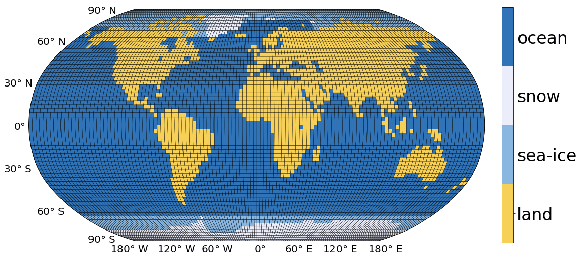
Figure 1Land, sea, and ice configuration with T42 resolution for 1950 CE as used in modern model runs and given by Zhuang et al. (2017a). Four surface types are differentiated: ocean, land surface, sea ice, and land-based ice or snow.
The model is solved on a T42 Gaussian grid with 128 points in longitude and 64 in latitude. In principle, other resolutions are possible, but since the resolution is defined at different points in the code, any change to the resolution needs to be carefully implemented. Each grid point is categorized as one of four surface types – ocean, land surface, sea-ice, or land-based ice or snow – as shown in Fig. 1 for a modern land–sea configuration. The geography does not contain information about altitude and remains constant throughout a model run. Transient runs with changing land, sea, and especially ice configuration are possible by regularly restarting the model with updated boundary conditions using the climatology from the previous run. Figures 6 and 7 present the structure of the model code, which will be discussed in Sect. 2.3.
2.2 Forcings and parameterization
Four broad categories of parameters exist: heat capacity, albedo, thermal conductivity, and outgoing radiation. Figure 2 shows a conceptualized view of the energy transport of the model with all model parameters and forcings.
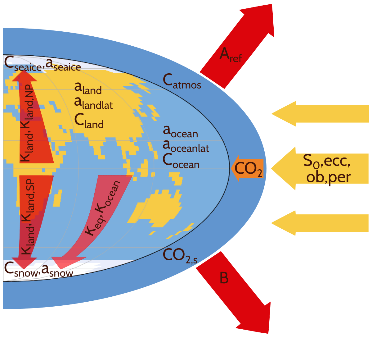
Figure 2Conceptual view of the forcings, energy transport, and parameterizations in TransEBM. Solar insolation S0, the orbital parameters, – eccentricity, obliquity, precession of the perihelion – CO2, land, sea, and ice distribution serve as forcings. The surface types differ by albedo a, which affects the insolation field, and heat capacity C. The energy from incoming solar radiation is transported poleward according to the thermal conductivities κ. The outgoing radiation is calculated based on the parameters A, B, and the response to CO2 scaled by CO2,s.
The simulated heat capacity changes with the surface type as listed in Table 1 and thus depends on the land, sea, and ice configuration. Due to this dependence, the heat capacity field remains constant during a single model run. For each grid point, the total heat capacity equals the sum of the heat capacity for its surface type and that of the atmospheric column above. For the atmospheric column an average scale height of 7.6 km is assumed. Zhuang et al. (2017a) base the oceanic heat capacity on the assumption of a mixed layer of about 70 m. This can be changed by tuning the oceanic heat capacity as presented in Sect. 2.4. The tuned heat capacity of TransEBM corresponds to a mixed layer of about 96 m.
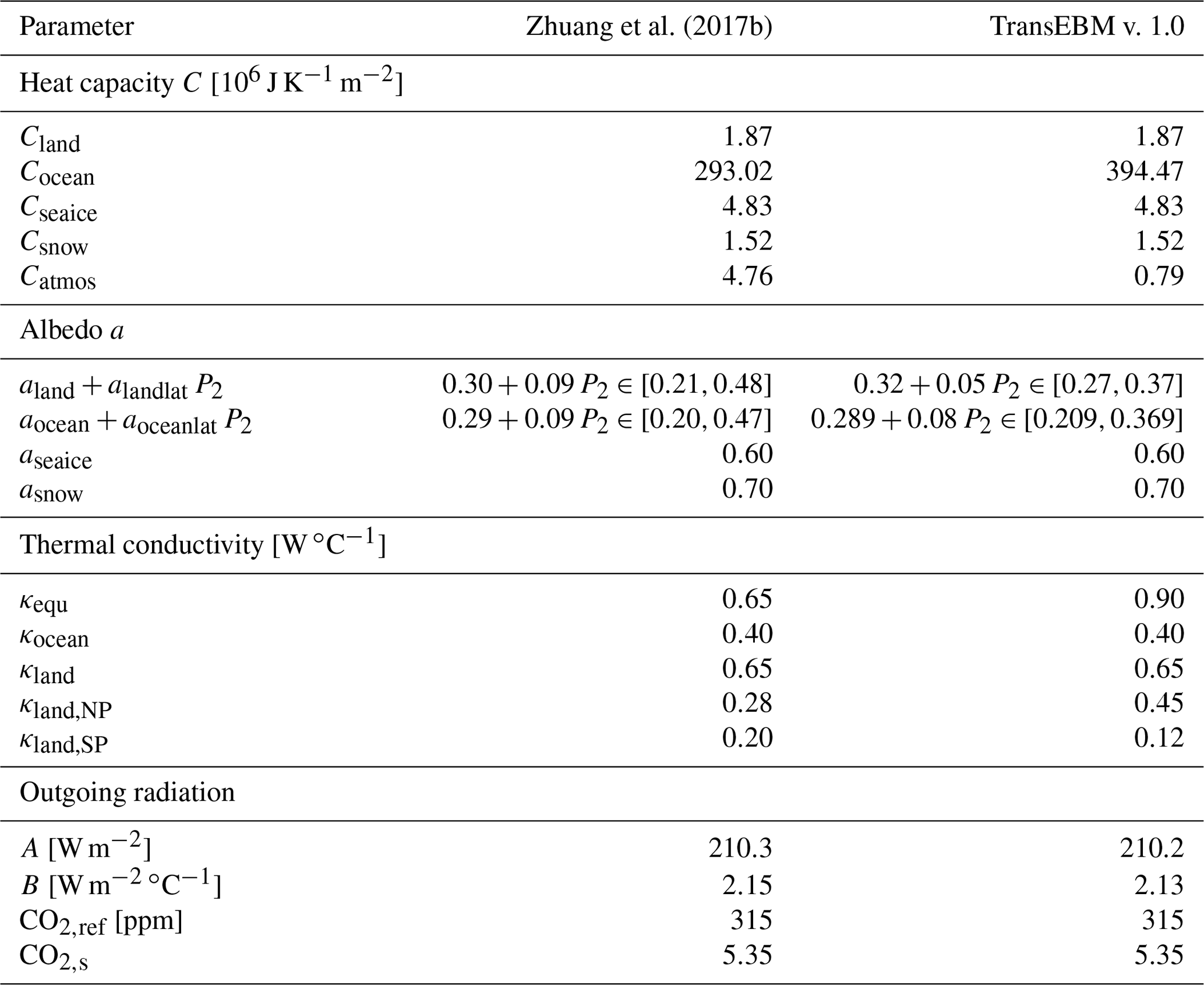
Zhuang et al. (2017b)Table 1List of all model parameters for the model by Zhuang et al. (2017b) and TransEBM v. 1.0 after the tuning described in Sect. 2.4. Albedo over land and ocean depends on latitude θ via the second Legendre polynomial .
Local relaxation timescales τ are determined by the total heat capacities in the atmospheric column over surface type i and the outgoing radiation coefficient B as . Table 2 lists the resulting relaxation times and shows that the longest timescales are simulated for the ocean at about 6 years. Therefore, the contribution of the deep ocean that impacts timescales on the order of 102 years and longer (Rohling et al., 2012) is not modeled. For the other surface types, relaxation times are far smaller and range from about 2 weeks to 1 month. Overall, the heat capacity parameters approximate the effect of energy storage in the climate system since TransEBM does not model energy storage explicitly.
Table 2Total heat capacities and resulting relaxation times τ for surface type i.

It is possible to differentiate surface types beyond those currently used in the model. In fact, additional surface types to distinguish between water reservoirs like the Pacific, Atlantic, and Indian oceans, as well as the Mediterranean Sea and inland seas exist for the parameterization of heat capacity. Using them, the impact of the deep ocean could be modeled more accurately. However, other parts of the parameterization like the albedo are not yet adapted for a larger number of surface types.
The albedo depends on the geography and gets initialized at the beginning of a model run and then remains constant. Table 1 lists the albedo values that are assigned to the different surface types. The albedo fields of land surface and ocean are latitude-dependent. Figure 3 shows the albedo distribution of a present-day continental configuration as seen in Fig. 1. The highest albedo values are in snow-covered areas and the lowest are close to the Equator. Modeled albedo values agree with the ranges found in literature (cf. Ruddiman, 2014).
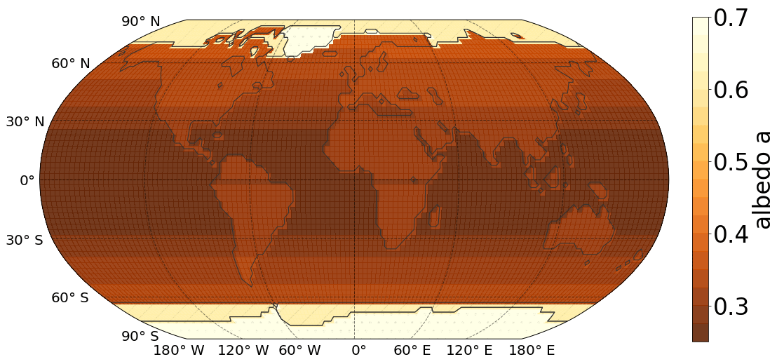
Figure 3Albedo field for the 1950 CE map shown in Fig. 1. Albedo differs by surface type. Over land and ocean it increases with latitude.
Heat transport due to sensible and latent heat, as well as oceanic heat transport across isotherms, is described using a heat transport coefficient
which is constant throughout one model run. Table 1 lists the values for the thermal conductivities κ, on which D depends. Figure 2 presents a conceptual view of the heat transport in the model. Oceanic heat transport is distinguished from heat transport over land and ice-covered areas. Over land and ice-covered areas, the Northern and Southern hemispheres are treated separately so as to reproduce differences in observed temperature patterns due to the asymmetric distribution and sizes of the land masses. This difference increases towards higher latitudes. Figure 4 shows the resulting latitude-dependent pattern of the heat transport coefficient. Heat transport is large close to the Equator and declines towards higher latitudes, where it evens out.
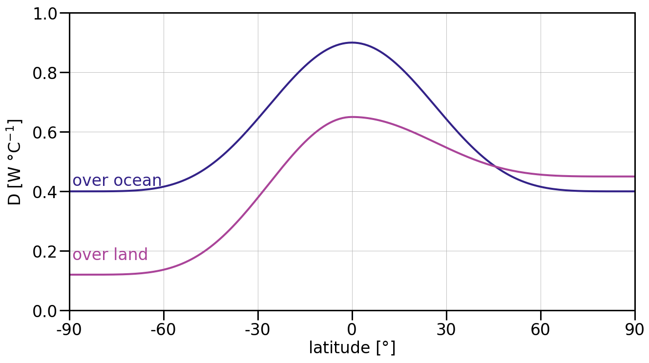
Figure 4Effective heat transport coefficient D as modeled in TransEBM v. 1.0 and computed from the thermal conductivities κ (cf. Eq. 2). Oceanic heat transport is treated separately from that over land and ice-covered areas. For the latter, the Northern and Southern hemispheres are separated, with larger heat transport coefficients in the north.
The parameterization of outgoing radiation as follows Budyko (1968) and uses phenomenological coefficients A and B. Both A and B were estimated from satellite observations in previous studies, but have large uncertainties attached to them (cf. Kyle et al., 1995; North and Kim, 2017). A captures the direct radiative effect of atmospheric CO2 on radiative forcing. Following Arrhenius (1896), Myhre et al. (1998) established its dependence on CO2 as
here with reference values Aref=210.2 W m−2 and ppm and scaling factor . Aref and CO2,ref are fixed parameters that are excluded from tuning. Changing them requires the model to be re-tuned due to their influence on the other radiative parameters. Overall, A follows the CO2 input and can change with each model year.
B describes the radiative damping due to climate feedbacks. It is set to B=2.15 W m−2 , well within the range of satellite measurements (Kyle et al., 1995; North and Kim, 2017). Table 1 summarizes the parameterization of outgoing radiation, which remains constant during a model run.
Insolation is the only component of the parameterization that changes for each time step with the seasonal cycle. It depends on the latitude- and time-dependent insolation S(θ,t) and the albedo via
Berger (1978) relates the insolation to the solar constant at the top of the atmosphere S0 and the orbital configuration, which are both transient forcings in the model, as
Here, the orbital configuration is given by declination δ, absolute hour angle of the Sun at sunrise and sunset H0, and the normalized Earth–Sun distance ρ is as follows:
which depends on eccentricity e and the positional angle of Earth on its orbit around the Sun ν as given counterclockwise from perihelion.
Figure 5 shows the relationship between orbital forcing, insolation, and the modeled temperature response. For the three orbital forcings eccentricity, obliquity, and precession, it shows the difference in insolation and temperature during northern summer between the possible extremes of the orbital forcings as listed in Table 3. When examining one orbital parameter, the other ones were set to their listed average values. The simulations were run in equilibrium mode with the tuned model (cf. Sect. 2.4), the land–sea mask as shown in Fig. 1, and constant CO2=315 ppm and S0=1362 W m−2.
Precession of the perihelion has the largest effect on the distribution of solar insolation and the resulting changes in temperatures, followed by obliquity. The effect of the changing eccentricity is the smallest. Larger eccentricity results in a global decrease in temperatures between May and July when perihelion is set to occur at vernal equinox in March. This means that the Earth will be farther from the Sun in northern summer with higher eccentricities. The effect is larger in the Northern Hemisphere, particularly in midlatitudes.
A large obliquity between May and July decreases insolation in the Southern Hemisphere and leads to an increase in the Northern Hemisphere. In the Southern Hemisphere, this effect is strongest in the midlatitudes, but disappears over high latitudes. In the Northern Hemispheres, insolation increases up to around 60∘ N, and then stabilizes in the high latitudes, leading to the largest increase in temperatures at high latitudes and over land in midlatitudes.
For the high precession simulation, summer solstice and perihelion coincide, leading to increased insolation and temperatures between May and July. Overall, the strongest increase in insolation occurs in northern low latitudes and midlatitudes and the highest increase in temperatures over Asia. Temperatures grow large over land and in the northern high latitudes. Appendix B examines the effect of the orbital parameters on insolation and temperatures further by repeating this analysis for November to January and annual averages. For all orbital parameters, the insolation and temperature patterns even out over the ice-covered regions near the poles.
Table 3Orbital parameter extremes used to examine the maximal influence that the parameters have on the modeled distributions of insolation and temperature as shown in Fig. 5. To examine the effect of one parameter, the other two were set to average values and an equilibrium simulation with land, sea, and ice configuration as in Fig. 1 and constant CO2=315 ppm and S0=1362 W m−2 was run.
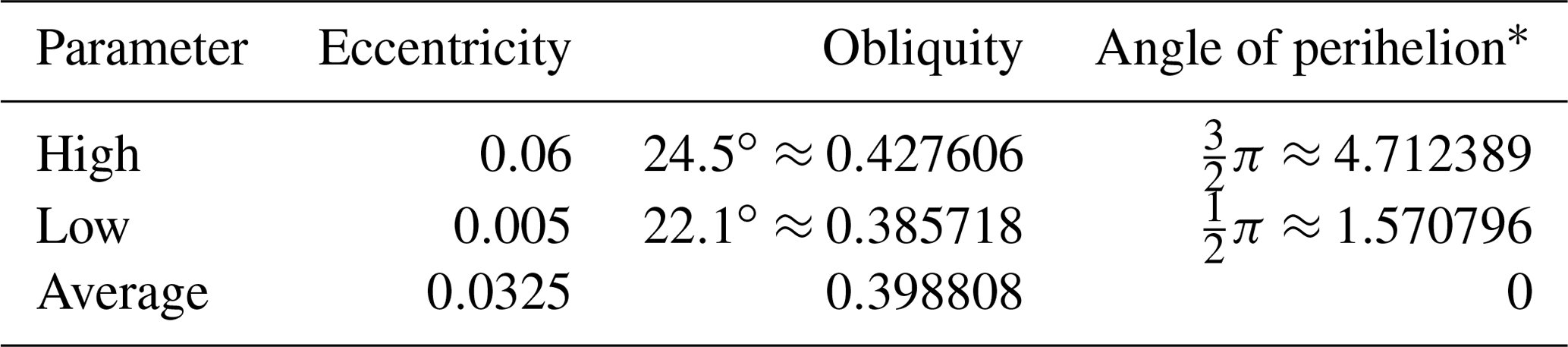
* Angle of perihelion is given from vernal equinox in TransEBM, so that 0∘, for example, means perihelion lies at the vernal equinox.

Figure 5Difference that high and low orbital parameters as listed in Table 3 cause in solar insolation (left) and temperature field (middle) for the averages of the months May, June, and July (MJJ). A schematic illustration of the orbital parameters is added to the right. Equilibrium simulations with land, sea, and ice configuration as in Fig. 1 and constant CO2=315 ppm and S0=1362 W m−2. (a–c) Eccentricity, (d–f) obliquity, and (g–i) precession of the position of perihelion. Precession shows the largest impact, followed by obliquity. High eccentricity results in overall lower insolation and temperatures; high precession overall resulted in increased insolation and temperatures. For eccentricity, decreased insolation in the north is found; for precession, on the other hand, insolation increases in the north. High obliquity results in increased insolation in the north and decreased insolation in the south. Precession acts strongest in lower and middle northern latitudes; obliquity and eccentricity, on the other hand, affect the high latitudes the most.
2.3 Model extension and benchmarking
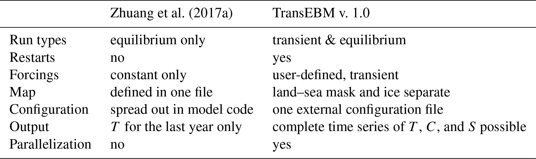
Based on the model code by Zhuang et al. (2017b), the model formulation was extended to enable transient and parallel runs, as well as transient, user-defined forcings for CO2, solar insolation, and the orbital configuration. The land, sea, and ice configuration can be changed within a simulation via model restarts at prescribed intervals. Additionally, the model configuration was overhauled so as to allow as much customization for experiments as possible. Table 4 summarizes the major expansions of TransEBM v. 1.0 with respect to the model by Zhuang et al. (2017a). A default configuration is provided with the model code. It contains detailed explanations for each variable that expand on the short tutorial provided in Sect. 4.
2017aTable 4Features of the revised model, TransEBM v. 1.0, in comparison to the model by Zhuang et al. (2017a).
The model has a preprocessing component visualized in Fig. 6 that imports the experiment's configuration, prepares the geography, and computes the albedo field. Based on this, the main component sets up the specified experiment, key steps of which are presented in Fig. 7. The initial setup is then integrated until either equilibrium or the user-defined number of years is reached. Finally, the output is written to netCDF files.
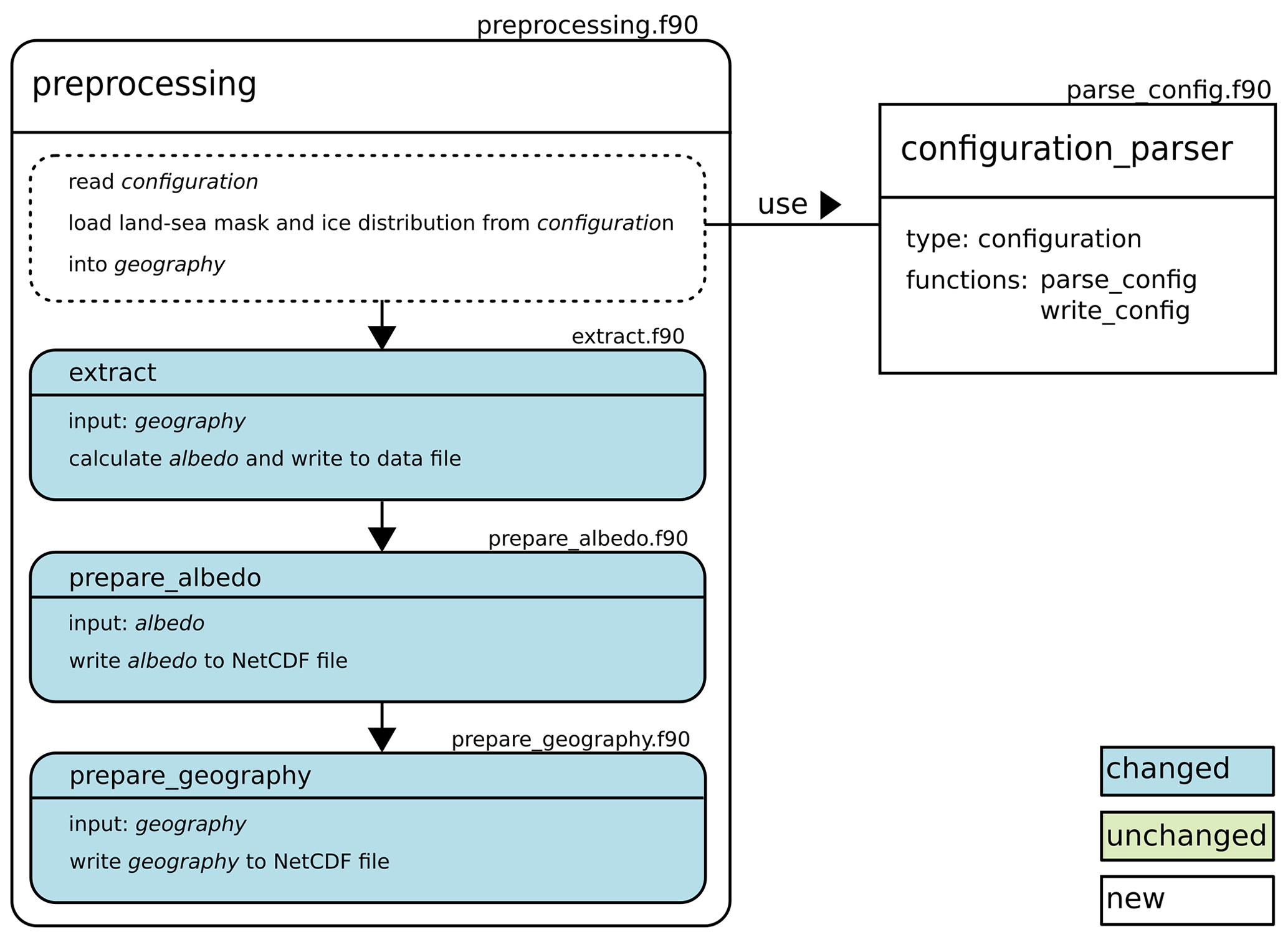
Figure 6Preprocessing component of the model with new, changed, and unchanged features with respect to the EBM by Zhuang et al. (2017a) marked.
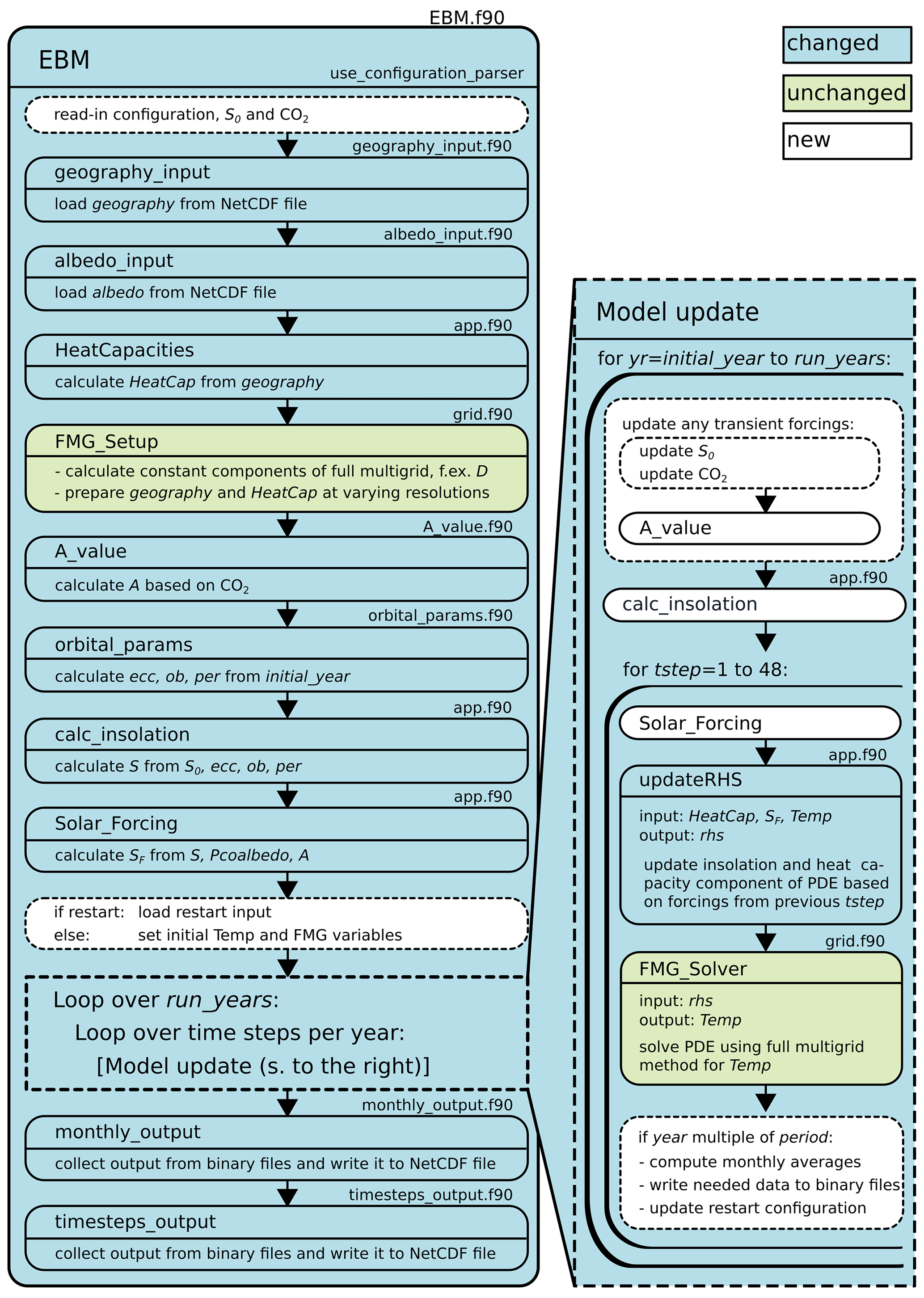
Figure 7Main model component with new, changed, and unchanged features with respect to the EBM by Zhuang et al. (2017a) marked.
Only the land, sea, and ice distribution – described in the map section of the configuration – is constant throughout a model run, all other forcings can be transient. For long-term simulations, changing it is essential. This can be achieved by restarting the model based on the restart configuration that is continually updated while running. Such restarts preserve the state of the model and allow for the user to manipulate the run as desired and restart it from any modeled year for which restart information was written. This restart information consists of the temperature and insolation fields in the last time step of the year from which to restart. In a restart, these fields are used as the input for Eq. (1), which is updated and solved using the changed forcings.
The model is written in Fortran 90 and uses bash scripts and CMAKE and as such should run on standard Linux or Unix machines. In equilibrium mode, it takes between 35 and 40 years to reach a steady state. For each simulated year, a minimum of 13 MB of output is created. On a 64-bit Ubuntu 18.04.2 LTS machine with a gfortran-7 compiler, simulating one model year takes 1.5 s on a single core of an Intel i5−8600K 3.6 GHz processor. This translates into the calculation of 57 600 years in a single day.
2.4 Tuning methodology
The model is tuned to the 1960–1989 climatology from ERA-20CM reanalysis (Hersbach et al., 2015). Target metrics are global mean temperature (GMT), the root-mean-square error of the latitudinal temperature distribution (RMSElat) and seasonal temperature distribution in the Northern Hemisphere (RMSEseas,nh) and Southern Hemisphere (RMSEseas,sh). An ensemble of simulations explores the parameter space with respect to these four metrics as shown in Figs. 8 and 9. These simulations model the same time period with 100 years beforehand to ensure the decay of the transients. The land, sea, and ice configuration was constant and as shown in Fig. 1. Orbital parameters were also constant during the simulations with eccentricity (ecc =0.016740), obliquity (ob =0.409253), and longitude of perihelion (per =1.796257), while CO2 followed Köhler et al. (2017) and S0 followed Coddington et al. (2016).
To get a complete picture of how the parameters affect the modeled temperatures, parameter values that disagree with observations or physics were explored as well. During the actual tuning, however, only configurations that agree with observations and physics were considered.
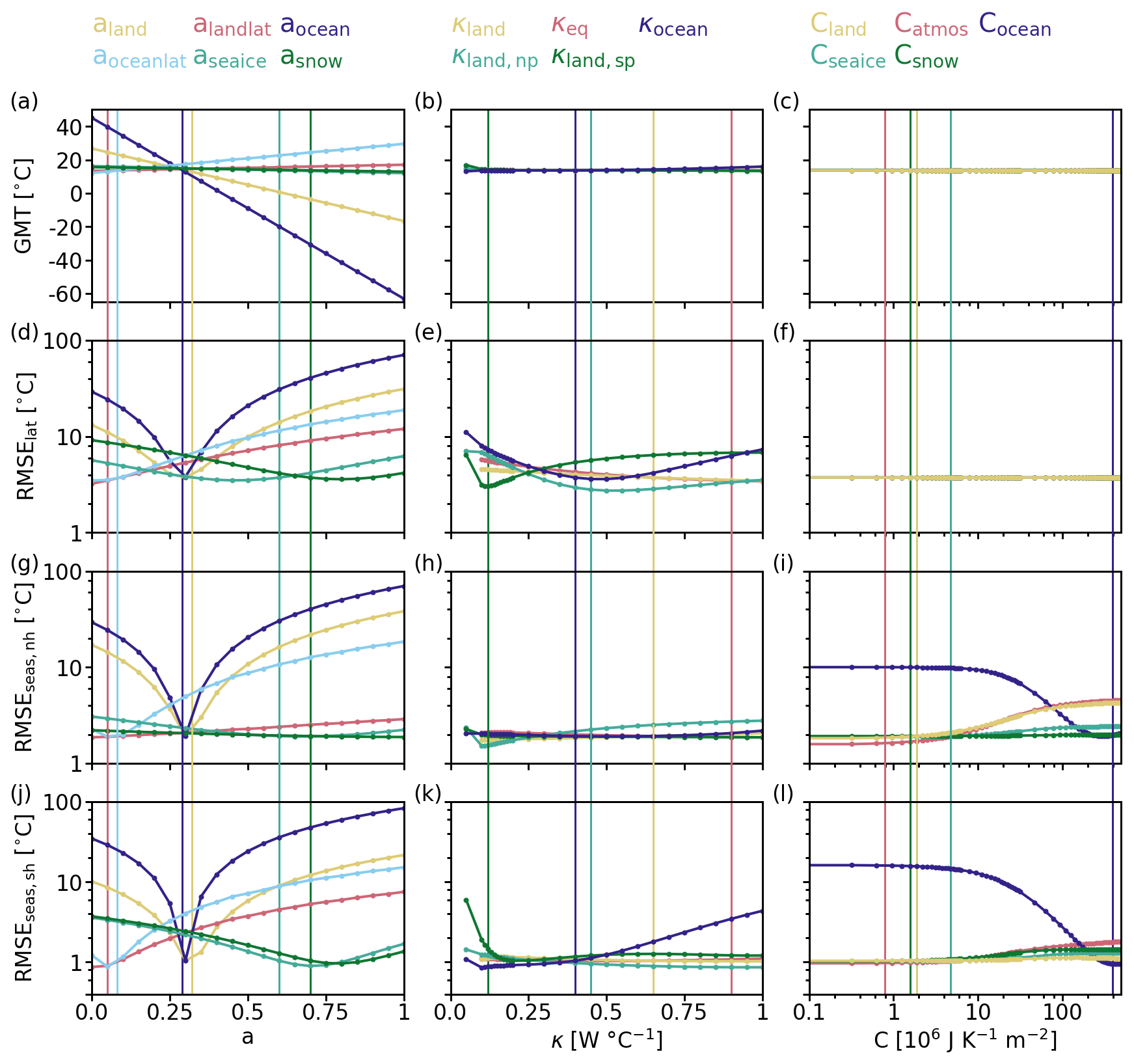
Figure 8Effect of changes to the parameterization of albedo (first column), heat transport (second column), and heat capacity (third column) on the GMT and the RMSE of the latitudinal (RMSElat) and seasonal temperature profiles in both hemispheres (RMSEseas,nh and RMSEseas,sh) with respect to ERA-20CM reanalysis (Hersbach et al., 2015). (a–c) GMT, (d–f) RMSElat, (g–i) RMSEseas,nh, and (j–l) RMSEseas,sh with all specific parameters listed at the top of each column. Simulations and reanalysis cover 1960–1989 CE. The simulations used the land, sea, and ice configuration shown in Fig. 1 and constant orbital parameters: eccentricity (ecc =0.016740), obliquity (ob =0.409253), and longitude of perihelion (per =1.796257). CO2 followed Köhler et al. (2017), and S0 values followed Coddington et al. (2016). Vertical lines indicate the chosen values after tuning. Albedo affects all tuning metrics, while thermal conductivities barely change GMT and heat capacities only manipulate the seasonal temperature distributions.
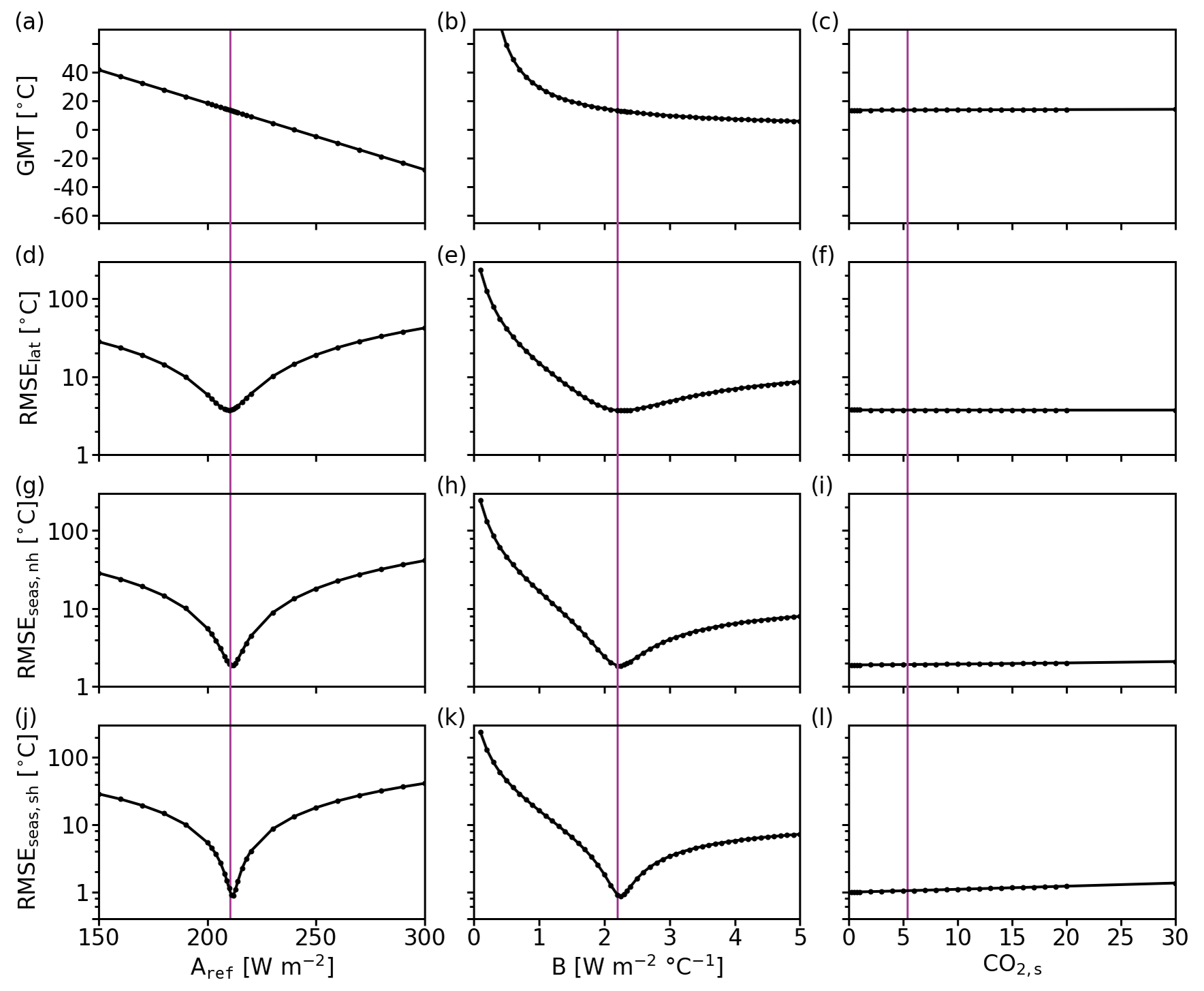
Figure 9Effect of changes to the parameterization of the outgoing radiation on the GMT and the RMSEs of the latitudinal (RMSElat) and seasonal temperature profiles in both hemispheres (RMSEseas,nh and RMSEseas,sh) with respect to ERA-20CM reanalysis (Hersbach et al., 2015). (a–c) GMT, (d–f) RMSElat, (g–i) RMSEseas,nh, and (j–l) RMSEseas,sh. The first column shows results for Aref, the second shows results for B, and the third shows results for CO2,s. Simulations and reanalysis cover 1960–1989 CE. The simulations used the land, sea, and ice configuration shown in Fig. 1 and constant orbital parameters: eccentricity (ecc =0.016740), obliquity (ob =0.409253), and longitude of perihelion (per =1.796257). CO2 followed Köhler et al. (2017), and S0 values followed Coddington et al. (2016). Vertical lines indicate the chosen values after tuning. GMT reaches up to 257 ∘C for B; for a better comparison to the other parameters, the full range is not shown in panel (b). Both A and B affect all tuning metrics, whereas changes in CO2,s barely make a difference.
Albedo changes have a strong effect on temperature means and extremes and as such affect all metrics as seen in Fig. 8. They do not influence the shapes of the seasonal temperature distribution though, since the albedo field is constant throughout the model year and as such affects the insolation at all time steps the same way. The thermal conductivities κ describing the heat transport primarily alter the seasonality and Equator-to-pole gradient. Decreasing them sharpens the latitudinal distribution and increases the seasonality and vice versa for increased thermal conductivities. In comparison to albedo, they have a small effect on global mean temperature and produce differences of about 5 ∘C over the whole explored parameter space. Changing the heat capacities affects the equilibration time and the seasonal cycle, both in regard to the lag of the temperature response to the forcing and the absolute temperature difference between warmest and coldest month. Figure 9 shows that the outgoing radiation parameters Aref and B influence GMT, the latitudinal distribution, and seasonality. By comparison, CO2,s only has a small effect on the seasonal distribution.
Table 5List of the parameter groups and which of the tuning metrics (GMT, RMSElat, and RMSEseas) they affect based on the results shown in Fig. 8 and 9. Bracketed markers (x) represent a notably smaller but not negligible influence by that parameter on the tuning metric in comparison to the other parameters.
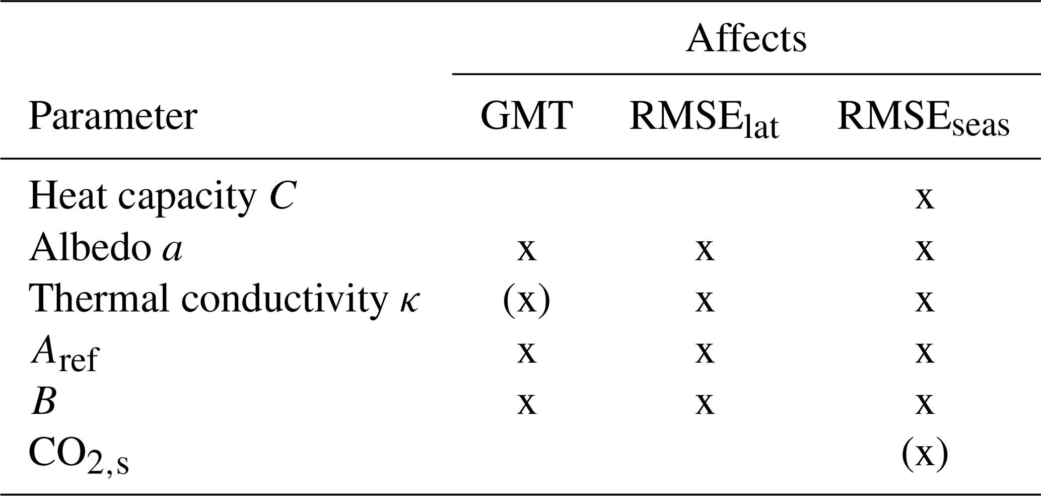
Table 5 summarizes which parameters affect which metric. It shows that only the seasonal distribution can be tuned without affecting the other metrics. Minimizing the root-mean-square errors was prioritized over agreement with the GMT from ERA-20CM GMTERA=13.27 ∘C. With respect to GMT, any tuning options were only discarded if they produced a change in GMT of 2∘ or more. The latitudinal and seasonal distributions were prioritized to ensure that the spatially resolved temperature fields show realistic features. Moreover, the latitudinal and seasonal profiles deviated considerably from observations in areas of interest (e.g., the polar regions), whereas the GMT was already very close to that found in the ERA climatology. However, depending on the envisioned applications, the relative weighting of the tuning metrics could change. Since RMSElat was the highest, with significant disagreement observed in the polar regions, it was the initial focus of the tuning. Table 6 shows the metrics before and after tuning. The agreement between the latitudinal distributions in ERA-20CM and TransEBM and the seasonal distributions in the Southern Hemisphere improved. RMSEseas,nh increased slightly, but since this produced a large improvement in the other two RMSEs, this increase was considered acceptable. Although GMT was barely considered during the tuning, the final GMT is closer to the target.
Table 6Tuning metrics GMT, RMSElat, and RMSEseas for each hemisphere before and after tuning. The metrics were evaluated for the years 1960–1989 CE against ERA-20CM (GMTERA=13.27 ∘C). The simulations used the land, sea, and ice configuration shown in Fig. 1 and constant orbital parameters: eccentricity (ecc =0.016740), obliquity (ob =0.409253), and longitude of perihelion (per =1.796257). CO2 followed Köhler et al. (2017), and S0 values followed Coddington et al. (2016). All metrics except RMSEseas,nh improved with tuning.

3.1 Tuning validation and comparison to EBM by Zhuang et al. (2017a)
The model was tuned using the 1960–1989 climatology of a simulation of the 20th century (1900–1989). As a first validation of that tuning, we compare that whole simulation to ERA-20CM reanalysis data (Hersbach et al., 2015) and a simulation with the EBM based on the parameterization by Zhuang et al. (2017a). Both simulations used the constant modern land, sea, and ice configuration shown in Fig. 1, with transient CO2 data from Köhler et al. (2017) and S0 values from Coddington et al. (2016). To follow the evolution of CO2 and S0, the tuning used the extension to transient forcings of the model.

Figure 10Comparison of a simulation of the 20th century using the parameterization by Zhuang et al. (2017a) with the tuned parameterization introduced in Sect. 2.4 and ERA-20CM reanalysis data (Hersbach et al., 2015). The simulations use the land, sea, and ice configuration from Fig. 1, CO2 is set according to Köhler et al. (2017), S0 follows Coddington et al. (2016) and orbital parameters Laskar et al. (2004). (a) Time series of the annual temperature anomaly from 1900–1989 CE with respect to the 1900–1929 climatological mean. The different parameterizations show little difference and capture the overall increasing trend, but the reanalysis shows stronger inter-annual variation. (b) The average latitudinal profile. Here, TransEBM agrees with reanalysis data better – especially in the polar regions and around the Equator. Seasonal temperature profiles in the Northern Hemisphere (c) and Southern Hemisphere (d) are both shifted in comparison to the reanalysis. Agreement is better in the Southern Hemisphere, TransEBM underestimates the seasonal cycle in the Northern Hemisphere.
Figure 10 summarizes the simulations and compares them to the reanalysis. Figure 10a presents the time series of the annual temperature anomaly and shows that both parameterizations produce very similar anomalies. They follow the overall increasing trend in temperatures that the reanalysis shows. However, the reanalysis shows a slightly larger increasing trend. The trend in the EBM is solely in response to the increasing CO2 values, so the difference indicates that the EBM is lacking positive feedback mechanisms that enhance the temperature response to increasing CO2, leading to the EBMs underestimating greenhouse-gas-related warming. Unlike the reanalysis, they also show smoother changes and less inter-annual variability. The 11-year solar cycle, which was superimposed, dominates inter-annual changes in GMT in the simulations.
Figure 10b presents the mean latitudinal temperature profiles. TransEBM agrees well with the reanalysis. In particular, it is able to simulate the dip in temperatures around the Equator and the temperatures in the polar regions better after tuning.
Figure 10c and d show the average seasonal temperature profiles in the Northern Hemisphere and Southern Hemisphere, respectively. The simulated average seasonal cycles lag in comparison to the reanalysis. The amplitude of the seasonal cycle is lower than that of the EBM by Zhuang et al. (2017a) as a result of the tuning.
For further analysis the phase lag was computed based on sinusoids fitted to the seasonal cycle for every grid box. The phase lag is computed as the difference between the occurrence of the extrema in the fit to the extrema in the insolation occurring on 21 June and 21 December. Figure 11 shows the resulting phase lags for TransEBM and ERA-20CM. Areas where the seasonal cycle does not follow a sine were excluded from the analysis. Appendix C provides details on the exclusion process. The resulting pattern in phase lags highlights that TransEBM produces larger lags. Over the oceans, the modeled phase lag is significantly higher than that in the reanalysis. Over land and ice, TransEBM simulates longer phase lags as well, but the difference to the reanalysis is smaller than in oceanic areas.
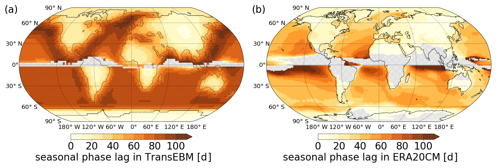
Figure 11Phase lag of the seasonal cycle in surface temperature in days after solar forcing (solstice) in a 20th century run of TransEBM v. 1.0 and ERA-20CM. The TransEBM simulation is the same as in Fig. 10. The phase lag uses sinusoids fitted to the seasonal cycle. Areas where the seasonal cycle does not follow a clear sine were excluded from the analysis and are shown in grey. TransEBM simulates larger phase lags in comparison to the reanalysis (particularly over the oceans).
The amplitude of the seasonal cycle is, on average, smaller in the EBM simulations in comparison to the reanalysis, especially in the Northern Hemisphere as seen in Fig. 10 and further examined in Fig. 12. In TransEBM the largest amplitudes of up to 40 d occur in Siberia and Antarctica. In the reanalysis, the largest amplitudes can be found in Siberia as well, although they are shifted in position in comparison to TransEBM. The reanalysis indicates high amplitudes in northern Canada as well. Overall, TransEBM agrees with the patterns in the reanalysis, and simulates rising amplitudes with increasing continental size and towards central continental areas and small amplitudes over the oceans. The patterns are smoother and less variable in comparison to those found in the reanalysis, though.
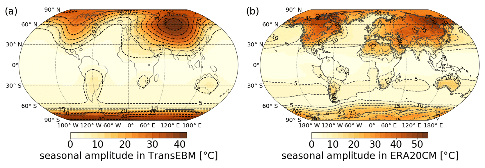
Figure 12Amplitude of the seasonal cycle in surface temperature during the 20th century in TransEBM v. 1.0 and ERA-20CM based on the extrema in the sinusoids fitted to the seasonal cycles. Simulation as in Fig. 10. TransEBM shows similar patterns to the reanalysis but simulates smaller amplitudes.
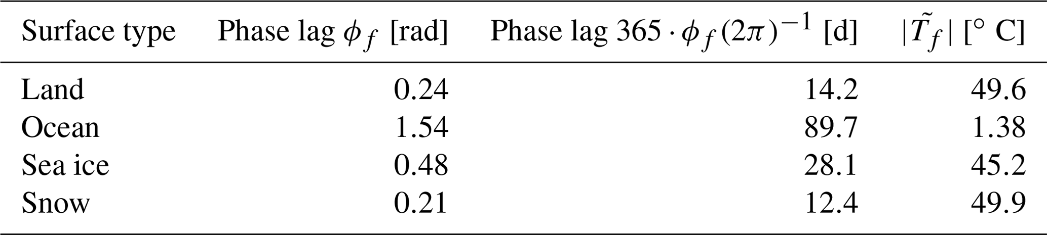
Following North and Kim (2017, chap. 2), theoretical average values for the amplitude and phase lag of the seasonal cycle in TransEBM can be calculated from the Fourier transform of Eq. (1). This yields the solution
with global mean albedo ag=0.32 for the present-day configuration shown in Fig. 3 and relaxation times τ for the specific surfaces as given in Table 2. The amplitude is then
and the phase lag in radians is
Table 7 presents the resulting amplitudes and phase lags for an annual forcing frequency d. The values corroborate the low oceanic seasonal amplitudes of only a couple of degrees and the much higher amplitudes over the other surfaces as shown in Fig. 12a. The phase lags also agree well with those found in the simulations (cf. Fig. 11a) with long average phase lags of about 90 d over the ocean and much shorter ones – between 2 weeks and 1 month – over the other surface types.
3.2 Sensitivity test
To test TransEBM's response to different forcings, we designed a three-step sensitivity test utilizing the implemented restarting extension. The model is initialized for conditions corresponding to the Last Glacial Maximum (LGM) with the forcings listed in Table 8. This simulation is run for 100 years with constant forcings. Following this, either one forcing or all of them shift to those found during the mid-Holocene warm period around 6000 years before present (BP). After another 100 years, the simulation switches to conditions for the year 2000 CE. Overall, the simulations thus cover three states in Earth's history with distinct climatic conditions that span a large range of the natural variability in forcings. For the solar constant there would be no significant change, which is why artificial steps were introduced that reveal its effect on the simulated climate. The simulation takes the orbital parameters for the three steps from Laskar et al. (2004) and CO2 from Köhler et al. (2017). For the land, sea, and ice distribution during the LGM and modern day, the data provided by Zhuang et al. (2017a) were used. They are shown in Fig. 1 and Fig. A1a, respectively. The map for the mid-Holocene warm period was then the result of an interpolation between the two based on the sea level reconstruction by Grant et al. (2012) and using the bathymetry by the National Geophysical Data Center (1993) (cf. Fig. A1b).
Table 8Step forcings for the sensitivity test. Modeled states are associated with the LGM, the mid-Holocene warm period 6000 BP, and 2000 CE. Orbital parameters follow Laskar et al. (2004), sea level w.r.t. 0 BP is from Grant et al. (2012), and CO2 is from Köhler et al. (2017). Appendix A shows the land, sea, and ice distributions corresponding to the sea levels of the three modeled periods. The solar constant is chosen such that it, like the other forcings, changes significantly.
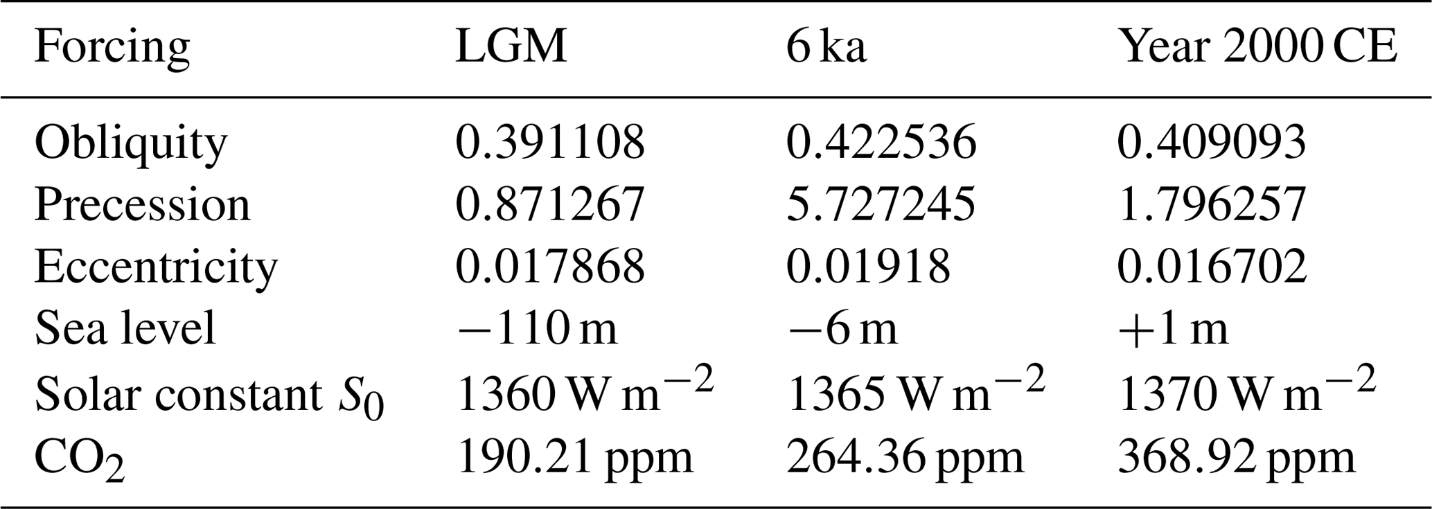
Figure 13 shows the temperature time series resulting from the sensitivity test. Among the forcings, the distributions of ice sheets and sea ice and the CO2 value have the largest effect on GMT. Despite its artificial enhancement, the solar constant has a smaller influence. Changes to the land–sea mask and to obliquity have a significant effect as well, whereas the variations due to eccentricity and precession are negligible. The sum of the temperature changes due to the individual forcing steps is slightly larger than the simultaneous change in all forcings, suggesting that the model contains some nonlinear behavior introduced by the restarts.
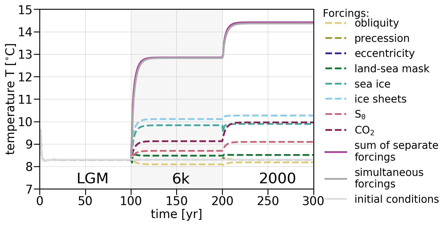
Figure 13Test of the sensitivity of the model to the different forcings. Conditions for three different states, which cover a large range in forcings, are simulated as described in Table 8. When forcings are applied one at a time, the sum of the temperature change differs slightly from when they act altogether, indicating some nonlinear model behavior. Changes to CO2 and the distributions of ice sheets and sea ice affect GMT the most.
3.3 Past millennium climate
To further examine TransEBM's abilities, we simulate the climate of the past millennium. The solar forcing includes the change in radiative forcing due to volcanic eruptions as given by Neukom et al. (2019), who also provided the CO2 forcing employed in this simulation. The orbital parameters are calculated according to Berger (1978) and the land, sea, and ice distribution is that from Fig. 1. To ensure adequate time for the decay of the transient solution, the simulation is initialized at 800 CE, but evaluated from 850 to 2000 CE. Figure 14 compares the results to a HadCM3 (Gordon et al., 2000; Pope et al., 2000) experiment (ID ∘xnapa', unpublished data, Kira Rehfeld, Bühler et al., 2020), a past millennium simulation with pre-industrial orography; solar, volcanic, and orbital forcing; and varying greenhouse gases. The temperature fields were regridded to T42 resolution. For the comparison of the GMT time series, the temperature reconstructions by the PAGES 2k Consortium (Neukom et al., 2019), as well as a CESM past millennium ensemble (Otto-Bliesner et al., 2016), were added.
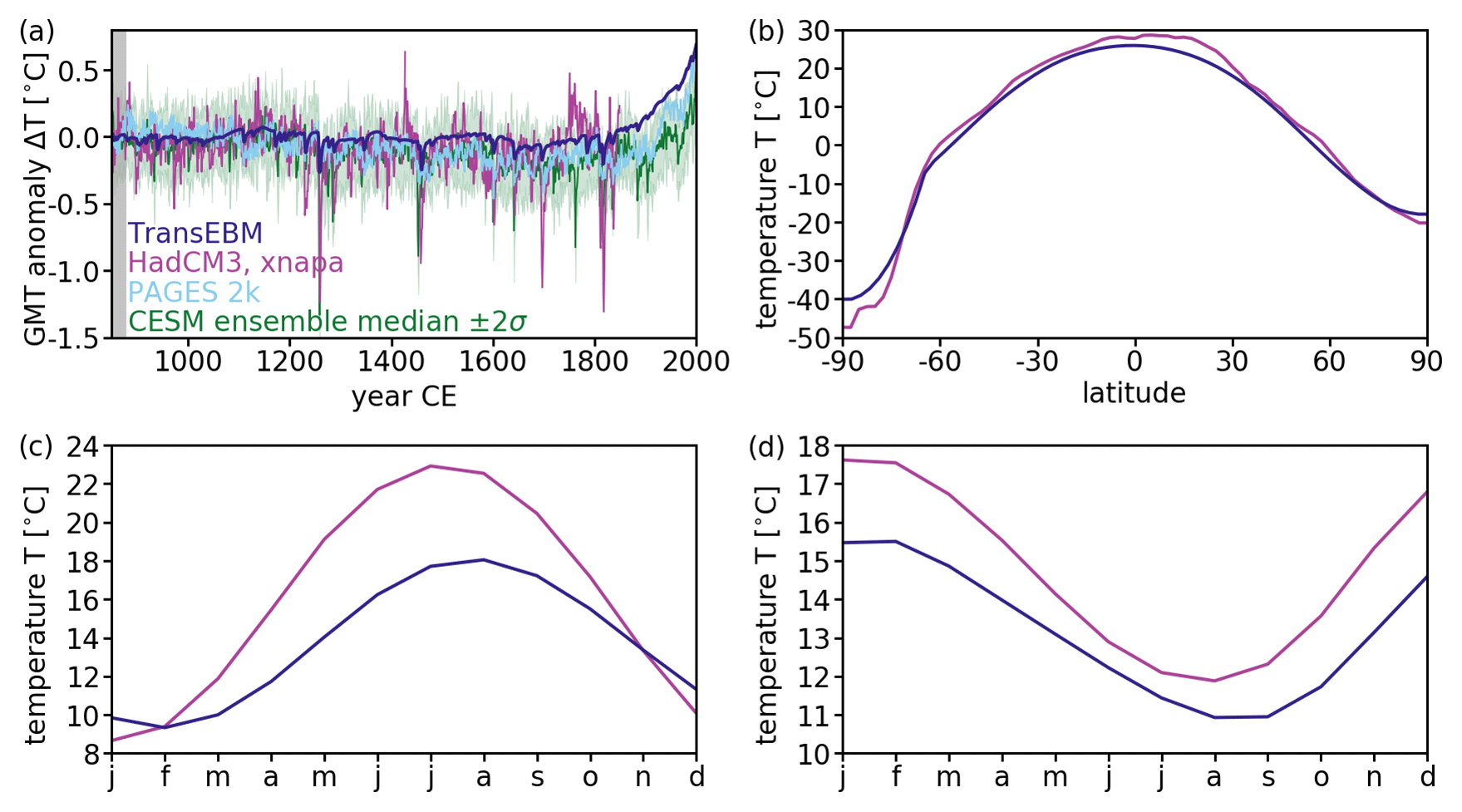
Figure 14Past millennium simulations and reconstruction. Solar, volcanic, and greenhouse forcings for TransEBM are from Neukom et al. (2019); orbital are parameters set according to Berger (1978); and land, sea, and ice distribution are the same as in Fig. 1. For comparison, the xnapa experiment (ID ∘xnapa', unpublished data, K. Rehfeld, Bühler et al., 2020) from HadCM3 (Gordon et al., 2000; Pope et al., 2000) is provided until 1850 CE, in addition to GMT in a CESM ensemble (Otto-Bliesner et al., 2016) and a reconstruction for the Common Era (Neukom et al., 2019). Panel (a) presents the GMT anomaly with respect to the climatological means from 850 to 879 CE. For CESM, the ensemble median with a spread of 2 standard deviations is shown. The grey shading indicates the reference period. Panel (b) shows the average latitudinal temperature profiles; panels (c) and (d) show the average seasonal temperature profiles for the Northern Hemisphere and Southern Hemisphere, respectively. The overall trends in GMT agree, but HadCM3, CESM and the reconstruction are much more variable. Additionally, HadCM3 and CESM show a stronger response to volcanic forcing. The latitudinal profiles show disagreement only over Antarctica and in the lower latitudes of the Northern Hemisphere. The seasonal cycles disagree, with HadCM3 simulating overall higher temperatures and a larger amplitude in the Northern Hemisphere.
Figure 14a presents the temperature anomalies. As in the 20th century simulations, the overall trends are similar, but TransEBM simulates lower variability than HadCM3 and CESM. The reconstruction also shows larger variability. The response from HadCM3 and CESM to volcanic forcing, seen for example in large negative peaks, is also larger than in TransEBM. As discussed in Sect. 3.1, this is most likely due to a lack of positive feedback mechanisms in TransEBM, which are present in the more detailed descriptions of HadCM3 and CESM. The response to the increase in greenhouse forcing, on the other hand, is similar in TransEBM, CESM, and the reconstruction. The average latitudinal distributions shown in Fig. 14b largely agree. They differ over Antarctica, where HadCM3 simulates lower temperatures, and in the lower latitudes of the Northern Hemisphere, where HadCM3 produces higher temperatures. The seasonal cycles in the Northern Hemisphere and Southern Hemisphere as displayed in Fig. 14, on the other hand, show significant disagreement: in the Northern Hemisphere the amplitude of the cycle is larger by about 5∘ in HadCM3, due to higher summer temperatures. In both hemispheres, the temperature extreme between July and September is shifted, with TransEBM lagging behind HadCM3. In the Southern Hemisphere, HadCM3 generally yields higher temperatures.
For setting up TransEBM, three files need to be potentially changed: preprocess/preprocess.sh, config/config_module.sh, and src/Makefile. The model was tested with Ubuntu 18.04 and the gfortran compiler and should run on Linux and Unix machines. To set up the model, follow the following procedure:
-
Start by installing all necessary packages. Running TransEBM requires Fortran90 or higher and NetCDF1. The optional post-processing relies on climate data operators (CDO, , ).
-
For using a compiler other than gfortan-7, change the compiler name in files config/config_module.sh, preprocess/preprocess.sh, and src/Makefile.
-
Set the paths to the local installation of NetCDF for Fortran in preprocess/preprocess.sh and src/Makefile via the following steps.
-
In preprocess/preprocess.sh, give the include path via I/usr/include and the library via the -lnetcdff flag. If the installation did not set that flag, provide the path via L/.../netcdf/lib instead.
-
In src/Makefile, provide the include folder via the variable NI and the library as the -lnetcdff flag. Give the compiler as FC=gfortran-7. Additionally, the configuration folder needs to be provided as I/home/user/TransEBM/config. Set this to the path of the configuration folder of TransEBM for the given setup.
-
-
To switch on the post-processing, un-comment the line
bash postprocess_cdo.sh $EBM_wrk _dir
in run_ebm.sh in the top level folder.
An experiment can be set up with a configuration file. The model code includes a default configuration in config/default_config.conf, which contains all variables that can be set, as well as a short explanation for all of them. The default configuration is that of an equilibrium experiment starting in 1950 CE with constant CO2=315 ppm, solar insolation S0=1362 W m−2, and orbital parameters. It uses the land–sea mask shown in Fig. 1, which is provided in the same folder, and the parameterization described in Sect. 2.4. To design a different experiment, TransEBM requires a configuration file that specifies all desired variables that differ from the default values. Any variables that are not set in that configuration will default to the values given in config/default_config.conf. Possible changes are as follows.
-
Set the land–sea mask and ice distribution
Give the path to a text file containing the desired land–sea mask as the parameter WORLD. That text file should have 64 rows and 128 columns and contain a number for each grid point that describes the surface type: 1 for land, 2 for sea ice, 3 for land-based ice, and 5 for ocean. It should contain no spaces or empty rows. -
Set the CO2 forcing
For a constant forcing, CO2_VALUE can be set together with CO2_FORCED = FALSE. For a non-constant forcing, a text file with one CO2 value per year and line can be provided as CO2_FILE with CO2_FORCED = TRUE and number of rows given as the file length CO2_FILE_LEN. -
Set the solar constant
Setting the solar constant works in exactly the same way as CO2 using the variable S0_VALUE with S0_ FORCED = FALSE for a constant forcing or S0_FILE with S0_FORCED = TRUE for a transient solar constant. Remember to set the file length in S0_FILE_LEN. -
Set the orbital parameters
For constant values, set ECC, OB, and PER or have them be calculated following Berger (1978). In the latter case, provide a start year of the experiment as INITIAL_YEAR and set ORB_SRC=”code” and ORB_ FORCED=TRUE. -
Define the length of the experiment
Provide the initial year as a Common Era value in INITIAL_YEAR, for example as 1950 or −21000 (relevant only if the orbital parameters are computed in the code). Set the number of years for which the simulation should be run as RUN_YEARS. -
Choose whether it is an equilibrium or transient simulation
For USE_EQUI=true, the experiment will be stopped once equilibrium or the number of RUN_YEARS is reached, whichever happens first. For USE_EQUI=false, the simulation will run for as many years as provided in RUN_YEARS. -
Set the working and the output directory
Set them using WRK_DIR and OUT_DIR. -
Set the experiment ID
Finally, the experiment should receive an ID.
Other possible changes to experiments include the option to change the parameterization and the writing of additional output. Once the configuration is set up, the model can be run by executing run_ ebm.sh with the following configuration file as input:
bash run_ebm.sh config/test.conf
If no configuration is specified, the code defaults to config/default_config.conf.
Building on previous modeling efforts, ranging from Budyko (1968) to Zhuang et al. (2017a), we have presented here TransEBM v. 1.0, a transient energy balance model that simulates Earth's temperature field based on CO2 greenhouse forcing, orbital parameters, and solar constant, as well as land, sea, and ice distribution. The provided tuning is in reference to the 1960–1989 climatology from the ERA-20CM reanalysis (Hersbach et al., 2015). It sampled the parameter space to investigate the sensitivity to the different parameters and, where available, relied on observations to provide boundaries. The tuning period and metrics, with a prioritization of the latitudinal and seasonal temperature profiles, were chosen to test the model's ability to simulate climate in polar regions and with its application for simulations of past climate in mind. The tuning improves the simulated seasonal cycle in the Southern Hemisphere and the latitudinal temperature profile in particular. Thereby, it improves the fit of the temperature profile in polar regions, showing that TransEBM can be used to model temperatures in ice-covered regions and as such provide ensemble runs exploring long timescales.
For the past millennium, there remain small disagreements with reanalysis and GCM simulations over Antarctica, where TransEBM overestimates temperatures towards the pole. This is due to the lack of topography in the model, which is why the elevation of ice sheets cannot be considered. Furthermore, the temperatures near the Equator disagree a little, with lower temperatures simulated by TransEBM for low northern latitudes. After tuning, TransEBM is able to reproduce the dip in temperatures related to the Intertropical Convergence Zone (ITCZ). However, this is an indirect parameterization of atmospheric dynamics that might not translate to climate states other than the tuned one.
TransEBM follows the overall trend in GMT but is unable to capture inter-annual variability due to the lack of dynamical processes modeled. With respect to the seasonal cycle, TransEBM lags the reanalysis data and produces smaller seasonal amplitudes. Moreover, there is less variability found in the spatial distribution of the amplitudes in the model, mirroring the findings of Hyde et al. (1989). The spatial structures of the amplitude and phase lag of the seasonal cycle that they found in their EBM are similar to the ones presented here (cf. Figs. 12 and 11). They also found reduced spatial variability in comparison to observations. The simulated phase lags are similar as well (cf. Fig. 11 here and Fig. 3a in Hyde et al. (1989)), but the amplitudes differ (cf. Fig. 12 here and Fig. 1a in Hyde et al., 1989). In better agreement with the reanalysis, TransEBM produces amplitudes roughly twice as high as Hyde et al. (1989).
The seasonal cycle in TransEBM is a product of only the seasonality in its insolation fields. As such, it lacks seasonality in the sea ice response, which would influence the parameterization of albedo, heat transport, and heat capacity as simulated by the model. The first trials of including such a seasonal sea ice cycle that could lead to the inclusion of dynamical ice sheets have been unsuccessful since they destabilize the numerical scheme. Such a change to the model therefore requires further research. Furthermore, the model does not currently explicitly consider energy conservation. This is especially relevant for interactive changes to the land, sea, and ice distribution between model restarts.
Overall, TransEBM makes large ensemble runs and long timescales accessible for exploration and can be used to design experiments with models more constrained by computational costs since TransEBM runs quickly with limited computational resources. As an easy-to-use climate model, it is suitable for use in education and for reproducing past studies with energy balance models for which no documented code exists (e.g., Hyde et al., 1989). In order to reproduce studies of hysteresis and abrupt transitions between ice-covered and ice-free states (cf. North et al., 1983; Mengel et al., 1988; Crowley et al., 1989; Short et al., 1991), an extension of the model with interactive ice sheets and sea ice would be necessary. When it comes to forcings, TransEBM underlines the sensitivity to ice configuration and CO2 forcing of simulated climates in comparison to other forcings, which have smaller impacts on temperatures. Furthermore, it illustrates the large impact that the parameterization of the outgoing radiation and the albedo fields of ocean and land masses have on the model results.
We describe a transient energy balance framework suitable for simulating planetary temperatures on long timescales due to its computational efficiency. The model can capture trends in the global mean temperature and simulates latitudinal temperature profiles that agree well with ERA-20CM reanalysis data (Hersbach et al., 2015) and HadCM3 (Gordon et al., 2000; Pope et al., 2000), a general circulation model. There are differences with respect to the seasonal cycle especially in the Northern Hemisphere related to the tuning of the model provided here. TransEBM v. 1.0 has a larger phase lag than that found in reanalysis, and the amplitude of the seasonal cycle in the Northern Hemisphere is smaller. Overall, it simulates less variable temperature fields than reanalysis, multi-proxy reconstructions, or more complex models due to its reduced complexity.
Among the modeled forcings, changes to the ice sheets, CO2 level, and the sea ice configuration are shown to influence the simulated climate the most. Among the parameters, the albedo fields of the oceans and land masses, as well as the parameterization of outgoing radiation, have the largest impact, as even small changes to these parameters can shift the model results significantly. With respect to the seasonality, the heat capacity of the oceans also carries some weight. The model behaves largely linearly, with only a small difference between the separate and simultaneous application of the forcings.
Desirable future improvements include the addition of a seasonal cycle in the sea ice, which currently remains constant during a model run. The inclusion of this seasonality is likely to improve the modeled seasonal cycle. Such a change to the model could encompass all ice masses and have them respond dynamically to the modeled temperature changes. For this to be physically reasonable, consideration of energy conservation within the model is necessary, which is especially relevant for the simulation of climate on long timescales with significant changes to Earth's ice masses. Overall, TransEBM v. 1.0 is accessible for large and long ensemble runs and thus can complement complex models, in particular for the study of the influence of orbital cycles and other radiative forcings on Earth's energy balance.
Figure A1 shows the land, sea, and ice configuration used for the sensitivity test presented in Sect. 3.2. Figure A1a shows the map for the LGM taken from Zhuang et al. (2017a). Figure A1b shows a map corresponding to the state at 6000 BP. For this, the sea levels from Grant et al. (2012) were taken and applied to the bathymetry by the National Geophysical Data Center (1993) to obtain a land–sea distribution. Based on the difference in sea levels between this time and both the LGM and modern configurations from Fig. A1a and 1, respectively, the difference in ice cover was interpolated. The amount of ice corresponding to the difference in sea level was removed from the LGM map according to a weighting. The weighting preferred the removal of ice closer to the Equator and at the borders of ice cover, that is ice with more ice-free neighbors. Ice was removed randomly if only a fraction of the ice with the same weighting needed to be removed. This interpolation is flawed – it ignores the height of ice sheets, energy conservation, and many more aspects – but for the idealized sensitivity test it suffices.
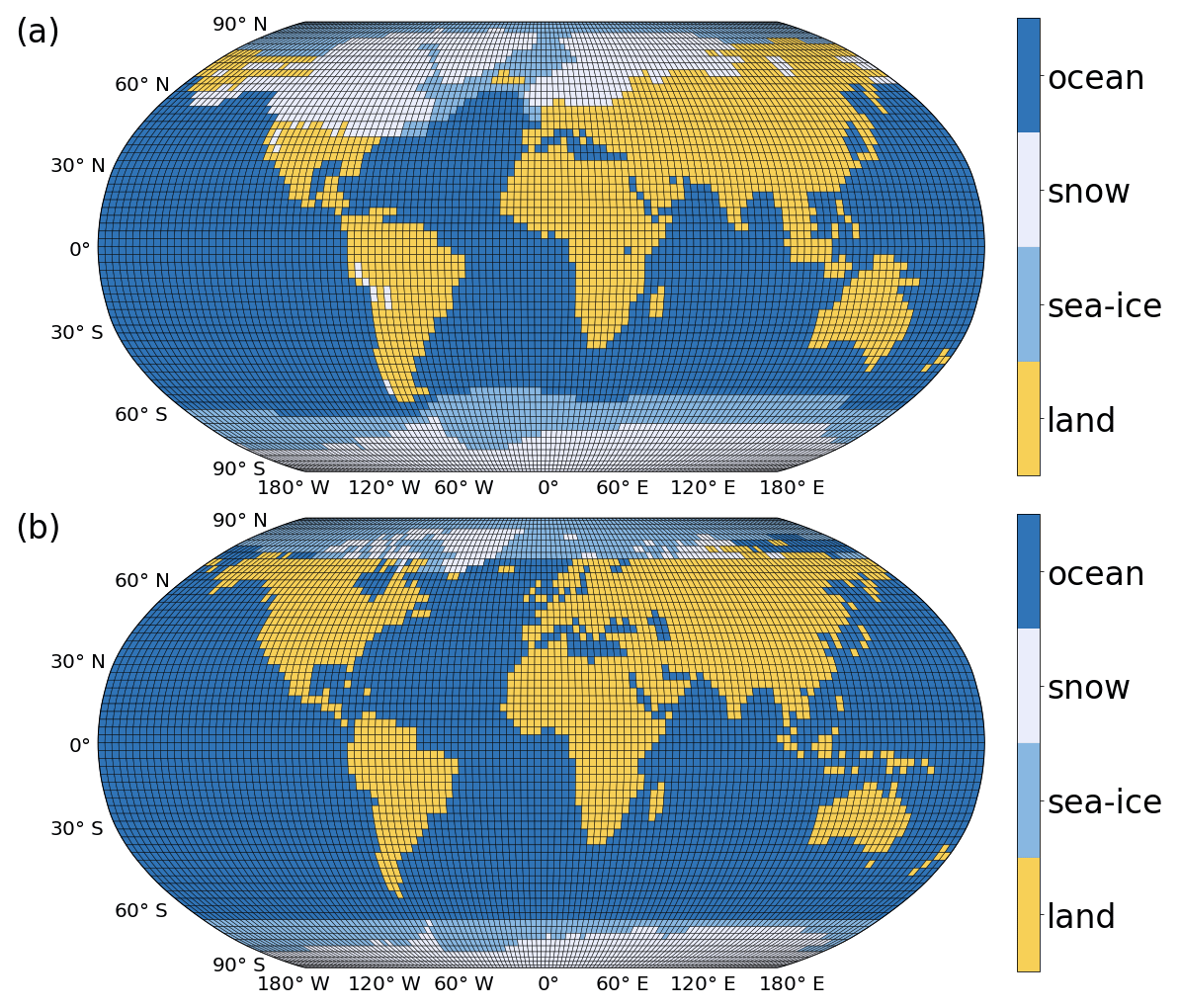
Figure A1Configuration of land, sea, and ice during (a) the LGM and (b) the mid–Holocene warm period about 6000 BP as they were used for the sensitivity test discussed in Sect. 3.2. Panel (a) is from Zhuang et al. (2017a); panel (b) has a land–sea distribution based on the sea level reconstruction from Grant et al. (2012) and the topography by the National Geophysical Data Center (1993). Ice was interpolated according to sea level difference of this state to (a) and the modern map from Fig. 1.
The relationship between orbital parameters and the modeled insolation and temperature distributions changes throughout the year. Section 2.2 analyzes the effect of extremes in orbital parameters on insolation and temperatures from May to July. Here, Fig. B1 repeats the same analysis for November to January. Overall, precession and obliquity cause similarly large differences in the amplitude of the insolation. For obliquity, this translates into the largest modeled temperature changes between low and high obliquity states among the three orbital parameters. Eccentricity, on the other hand, has the smallest effect both on insolation and temperatures.
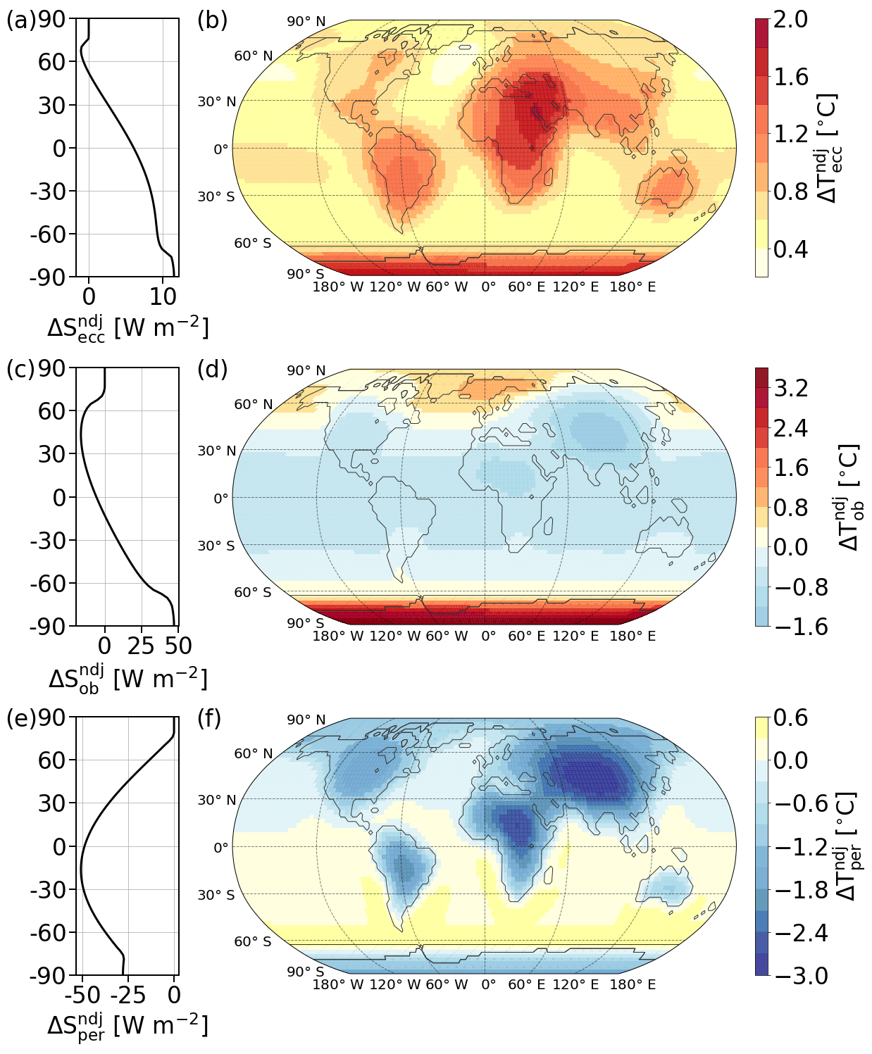
Figure B1Difference in solar insolation (left) and temperature (right) caused by extremes in the orbital parameters as listed in Table 3 for eccentricity (a, b), obliquity (c, d), and precession of the perihelion (e, f) from November to January (NDJ). Model configuration as in Fig. 14. Obliquity has the largest impact on simulated temperatures, closely followed by precession. High eccentricity corresponds to overall increased insolation and temperatures, with the largest increase in insolation towards the middle southern latitudes. Temperatures in the high eccentricity state change the most over Antarctica and continental areas near the Equator with respect to the low eccentricity simulation. A decrease in insolation in the Northern Hemisphere and increase in the Southern Hemisphere characterizes the high obliquity state when comparing it to the low obliquity one. Temperature increases are found in the polar regions, especially over Antarctica. Changes to precession have the strongest impact on low-latitude insolation and on temperatures in continental areas. NDJ insolation and temperatures are larger when perihelion occurs at the December solstice.
All three orbital parameters show a pattern mirrored between the hemispheres from that between May and July shown in Fig. 5. For eccentricity this means that a high eccentricity corresponds to larger insolation and temperatures than are found for a lower eccentricity if obliquity and perihelion are set to the averages noted in Table 3. This net positive effect is larger in the Southern Hemisphere with insolation growing towards middle southern latitudes. The largest increases in temperature are found over Antarctica, followed by a region covering eastern Africa and the Middle East. Altogether, temperatures increase the least over the oceans.
A high obliquity causes a decrease in insolation in the Northern Hemisphere and an increase in the Southern Hemisphere in comparison to the low obliquity simulation. The largest decrease can be found in the middle northern latitudes, and the largest increase can be found in the high southern latitudes. With regard to temperatures, the largest increase occurs in the southern polar regions, but increased temperatures are simulated for the northern polar regions as well. The largest decreases are found over Asia and near the Equator.
With the perihelion at the June solstice, insolation is lower between November and January in comparison to the perihelion occurring at the December solstice. This decrease is largest in the low latitudes of the Southern Hemisphere. It translates to decreased temperatures over land masses, Asia and Africa in particular, and towards the polar regions, which are affected by the lack of energy entering near the Equator, which, if present, would be transported polewards. Precession is the strongest in low southern latitudes, whereas obliquity and eccentricity affect the middle and high latitudes more.
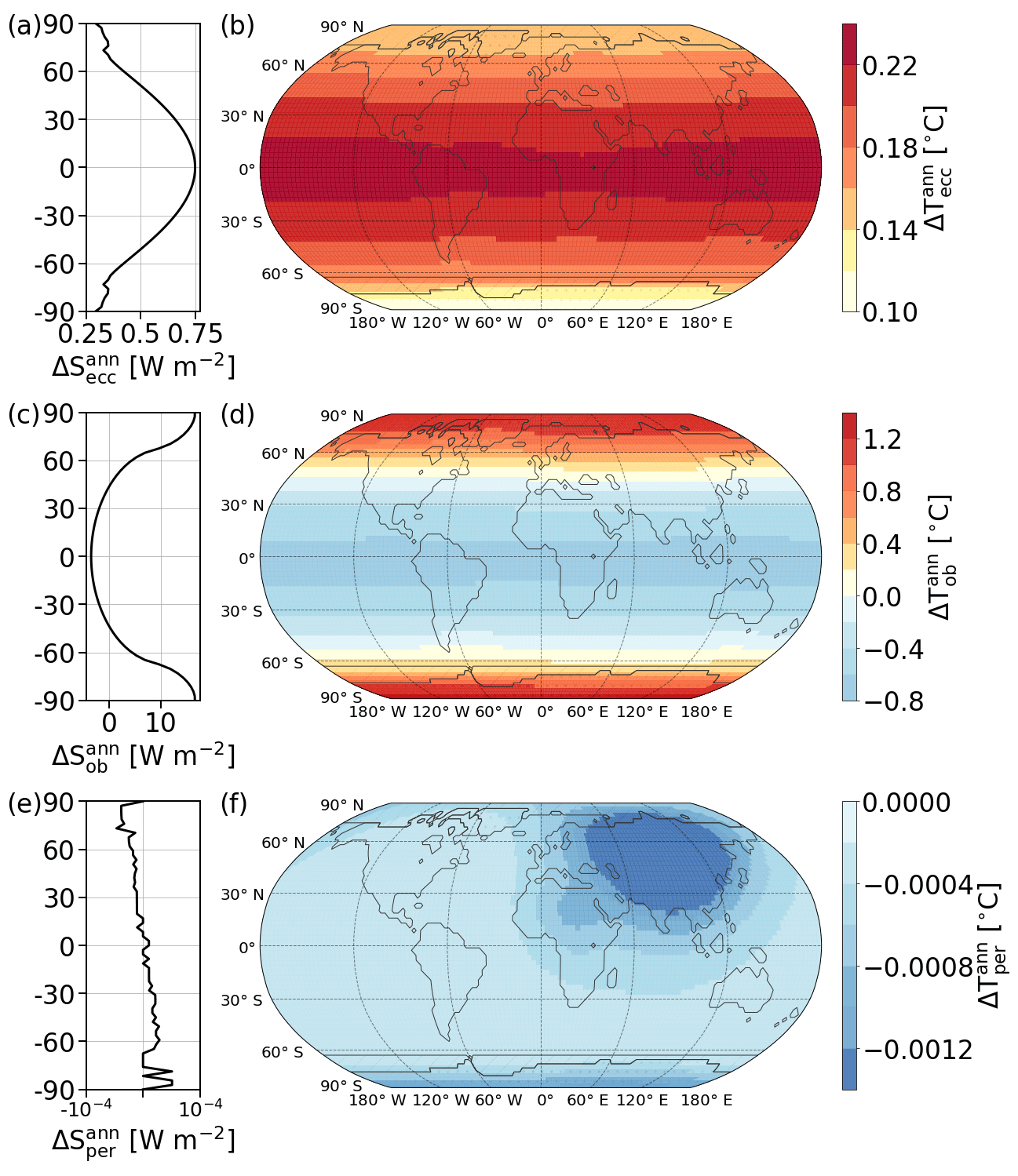
Figure B2Annually averaged difference in solar insolation (left) and temperature (right) caused by extremes in the orbital parameters as listed in Table 3 for eccentricity (a, b), obliquity (c, d), and precession of the perihelion (e, f). Model configuration is the same as in Fig. 14. Obliquity changes produce the largest difference, whereas the precession of the perihelion averages out throughout the year and has no effect on annual averages. Both eccentricity and obliquity show symmetric patterns. However, eccentricity affects the low latitudes the most, while the difference in the obliquity experiments grows polewards.
Repeating the analysis for yearly averages yields the results shown in Fig. B2. Most of the differences average out between the simulations with orbital extremes. For the precession of the perihelion in particular, there is virtually no difference between the experiments, as Fig. B2e and f show. Both eccentricity and obliquity show a symmetric pattern in the annual averages. The difference between obliquity extremes is the largest, confirming the results from the sensitivity study from Sect. 3.2, which also found that obliquity had the most notable effect on the global mean temperature among the orbital parameters. Obliquity affects the high latitudes the most, where a high obliquity increases insolation and temperatures. Close to the Equator, there is a net negative effect on the insolation and temperatures. A high eccentricity, on the other hand, produces the largest effect close to the Equator, with both insolation and temperatures decreasing towards higher latitudes.
The analysis of seasonality discussed in Sect. 3.1 fitted sinusoids to the detrended temperature time series of TransEBM and ERA-20CM for each grid box and then extracted the amplitude and phase lag from these fits. The computation of the phase lags relies on the fits, since TransEBM's low temporal resolution would only allow a coarse estimate. However, there are some grid boxes where such a fit oversimplifies the temperature pattern, especially in the ERA-20CM reanalysis. This is why the phase lag analysis shown in Fig. 11 excluded some grid boxes. Figure C1 delves deeper into these issues by showing the disagreement between the fitted amplitude and the amplitude calculated as the difference between the minimal and maximal temperature. The difference between the min–max and fit amplitudes serves as an indicator for how suitable the fit is for deriving amplitudes. The figure also shows the time series with fits for six exemplary grid boxes.
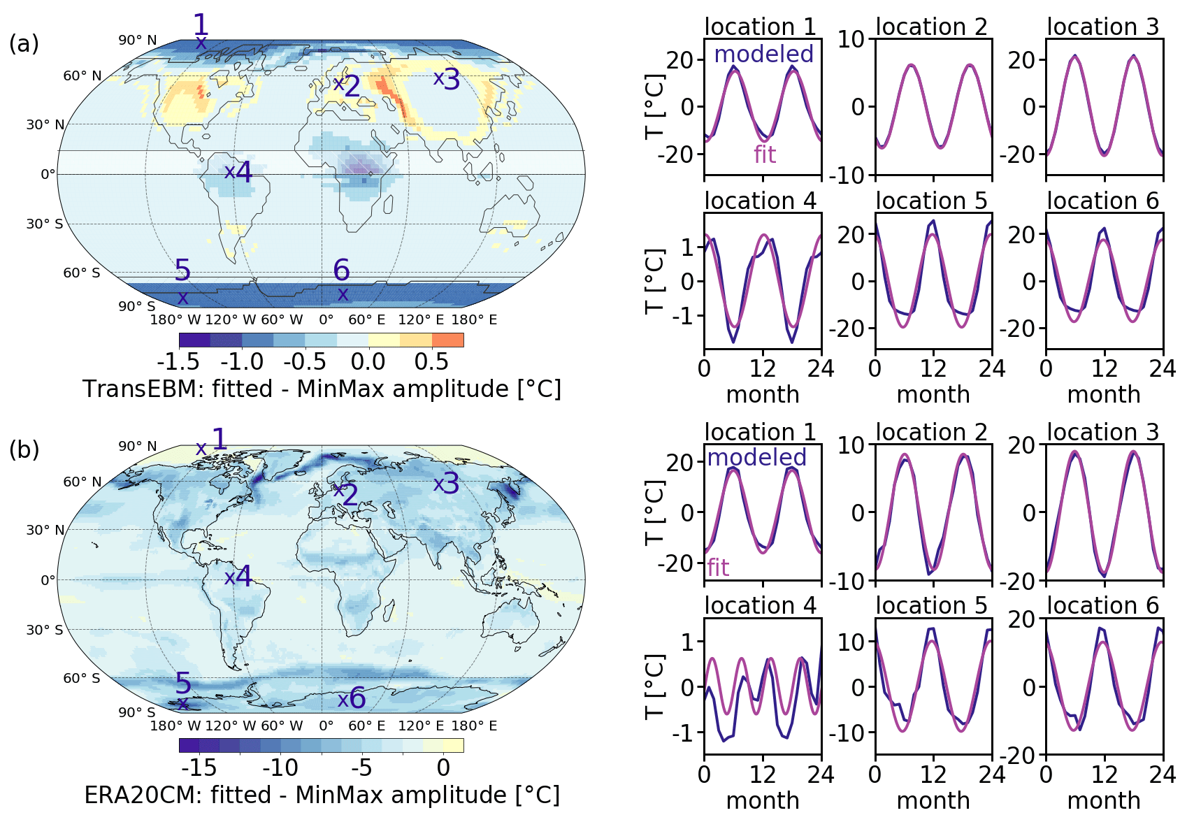
Figure C1Amplitude of the seasonal cycle extracted from fitting a sine minus the amplitude that results from taking the difference between the maximal and minimal temperature. Model configuration as in Fig. 5. Time series from (a) TransEBM and (b) ERA-20CM (Hersbach et al., 2015) from 1900 to 1989 CE, both were detrended. Six locations were picked as marked in the maps, for which 2 years of the time series and the fit are shown. For TransEBM, even the maximal differences are relatively small. In the polar regions the min–max amplitude is larger, over Asia and North America it is the other way around. For ERA-20CM the differences are larger, reaching up to around 15∘ in oceanic polar regions. The fit almost always produces smaller amplitudes. For both, locations 1–3 show places where the fit matches the time series very well. Location 4, on the other hand, lies close to the Equator inside the shaded area where the time series show only small variations throughout the year that are not sinusoidal. Locations 5 and 6 lie in Antarctica, where the fit is still applicable but is not able to fully capture the extrema.
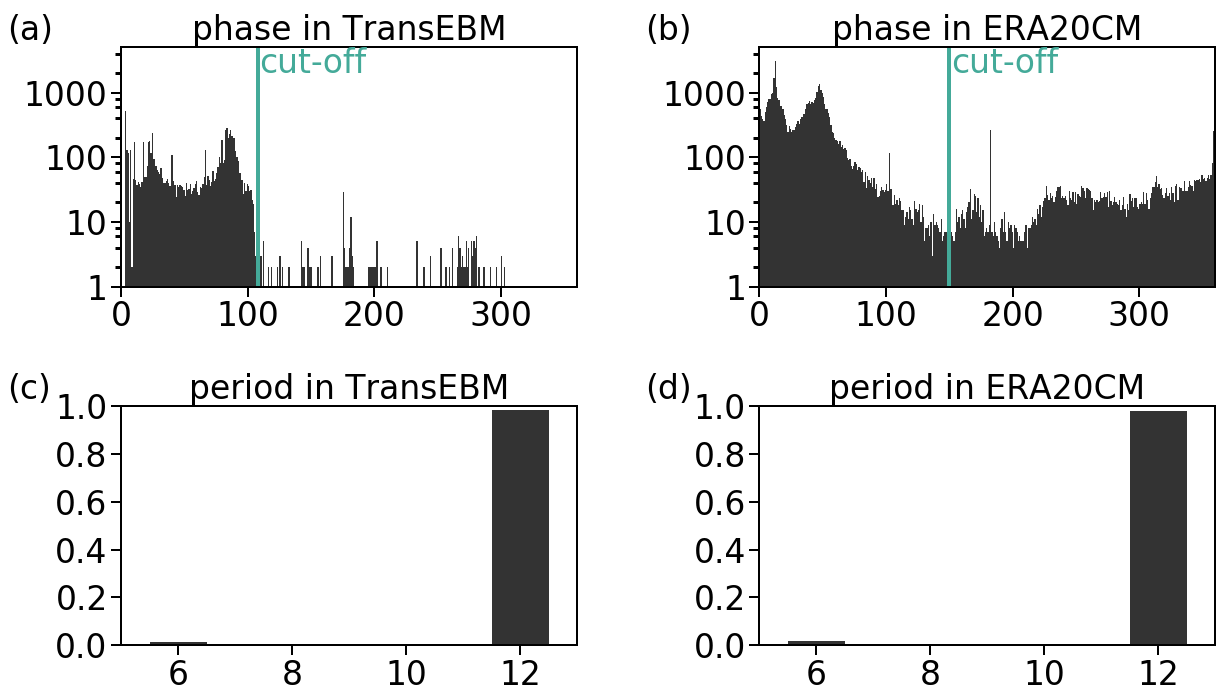
Figure C2Logarithmic histogram of the phase distribution in (a) TransEBM and (b) ERA-20CM (Hersbach et al., 2015) with cut-offs at 108 and 150 d, respectively, and histograms of the periods found in (c) TransEBM and (d) ERA-20CM. Both are based on the sinusoids fitted to the detrended 1900–1989 CE time series. Model configuration as in Fig. 5. Panel (a) shows a clear cut-off, after which only few grid boxes have larger phase lags. All of them lie close to the Equator, where the time series is not sinusoidal as shown in Figs. 12a and C1a. (b) In the ERA-20CM data a much larger variety of phases occurs and even very large phase lags are found. The cut-off here was chosen such that all locations close to the Equator with non-sinusoidal behavior were excluded. Many of the locations with very large phase lags are in Antarctica, where the temperature maximum sometimes occurs a couple of days before the insolation maximum as shown in Figs. 12b and C1b. Panels (c) and (d) both show that most grid boxes have a period of around 12 months, with very few exceptions of places where the fitted sine has a period of about 6.
Overall, the difference between the amplitudes is small in TransEBM. The fitted amplitude is larger by up to 1∘ over North America and parts of Asia. The min–max amplitude is larger in polar regions, as shown at locations 5 and 6 in Antarctica. In ERA-20CM reanalysis data the differences between the two types of amplitudes are larger, especially in locations with sea ice where they can become more than 15∘. It is notable that the fitted amplitude is almost always smaller and only ever larger by a little. This underestimation of the fitted amplitude is visible in locations 5 and 6, where the fit is unable to capture the temperature maxima. Location 4 near the Equator in South America is an example of a grid box that was excluded from the phase lag analysis. It is a location where the variations have a period smaller than 12 months. Since this was taken as a sign that a sine would not fit the underlying time series, such places where excluded from the analysis.
Figure C2 shows the histograms of the phases and periods for both TransEBM and ERA-20CM. A period other than around 12 occurs only in few places, mostly around the Equator where the time series shows no seasonal cycle. The phase histograms were used to define cut-offs to distinguish places where sine fitting was suitable from those, where the time series showed little or no sinusoidal behavior. Placing the cut-off is straightforward in TransEBM, since there is a gap at a phase lag of 108 d, after which there are almost no occurrences. Furthermore, Fig. 12a shows that all of these occurrences are close to the Equator, i.e., in places like location 4 without a 12-month seasonal cycle.
In ERA-20CM, the picture is more complicated, as Fig. C2b shows. Here, the cut-off was set by lowering it until all grid boxes close to the Equator where the time series is not suited to fitting a sine were excluded. This leads to a cut-off at 150 d. In doing so, large parts of Antarctica were excluded as well. As discussed previously in Sect. 3.1, these are places where the temperature maximum occurs slightly before the maximum in insolation, leading to very high computed phase lags, which the analysis omits. While this means that some grid boxes might have been excluded unnecessarily, this procedure allows confidence in all grid boxes that are included.
The current version of the model is available at https://github.com/paleovar/TransEBM (last access: 30 April 2021) and licensed under the GNU General Public License Version 3. The version of the model used for the analyses presented here is archived on Zenodo (https://doi.org/10.5281/zenodo.3941311, Ziegler and Rehfeld, 2020), together with all input data, configuration files, and scripts to run the model. The model simulations and all other data to produce the plots of this paper, as well as the code that generated the plots, are archived there as well.
EZ and KR conceptualized this study, decided on the methodology, created the analyses, and edited and reviewed the manuscript. EZ implemented the software and computations, performed the visualization of the data, and wrote the manuscript, all supervised by KR.
The authors declare that they have no conflict of interest.
We are grateful for discussions with Marie-France Loutre regarding our analyses and for the support by the Heidelberg Graduate School for Physics (HGSFP). We thank Beatrice Ellerhoff and all reviewers for their helpful comments on the manuscript.
This research has been supported by the Deutsche Forschungsgemeinschaft (grant no. 395588486), the Bundesministerium für Bildung und Forschung (grant no. 01LP1926C), the data storage service SDS@hd, supported by the Ministry of Science, Research and the Arts Baden-Württemberg (MWK) and the German Research Foundation (DFG) (grant no. INST 35/1314-1 FUGG).
This paper was edited by Andrea Stenke and reviewed by Colin Zhuang, Shaun Lovejoy, and one anonymous referee.
Abe-Ouchi, A., Saito, F., Kawamura, K., Raymo, M. E., Okuno, J., Takahashi, K., and Blatter, H.: Insolation-driven 100,000-year glacial cycles and hysteresis of ice-sheet volume, Nature, 500, 190–193, https://doi.org/10.1038/nature12374, 2013. a
Andres, H. J. and Tarasov, L.: Towards understanding potential atmospheric contributions to abrupt climate changes: characterizing changes to the North Atlantic eddy-driven jet over the last deglaciation, Clim. Past, 15, 1621–1646, https://doi.org/10.5194/cp-15-1621-2019, 2019. a
Arrhenius, S.: On the Influence of Carbonic Acid in the Air upon the Temperature of the Ground, Philosophical Magazine and Journal of Science, 41, 237–276, 1896. a, b
Bathiany, S., Dijkstra, H., Crucifix, M., Dakos, V., Brovkin, V., Williamson, M. S., Lenton, T. M., and Scheffer, M.: Beyond bifurcation: using complex models to understand and predict abrupt climate change, Dynamics and Statistics of the Climate System, https://doi.org/10.1093/climsys/dzw004, 2016. a, b
Berger, A. L.: Long-Term Variations of Daily Insolation and Quaternary Climatic Changes, J. Atmos. Sci., 35, 2362–2367, https://doi.org/10.1175/1520-0469(1978)035<2362:LTVODI>2.0.CO;2, 1978. a, b, c, d
Braconnot, P., Harrison, S. P., Kageyama, M., Bartlein, P. J., Masson-Delmotte, V., Abe-Ouchi, A., Otto-Bliesner, B., and Zhao, Y.: Evaluation of climate models using palaeoclimatic data, Nat. Clim. Change, 2, 417–424, https://doi.org/10.1038/nclimate1456, 2012. a
Briggs, W. L., Hensen, V. E., and McCormick, S. F.: A Multigrid Tutorial, Society for Industrial and Applied Mathematics, 2nd Edn., https://doi.org/10.1137/1.9780898719505, 2000. a
Budyko, M. I.: The effect of solar radiation variations on the climate of the Earth, Tellus, 21, 611–619, https://doi.org/10.3402/tellusa.v21i5.10109, 1968. a, b, c, d
Bühler, J. C., Roesch, C., Kirschner, M., Sime, L., Holloway, M. D., and Rehfeld, K.: Comparison of the oxygen isotope signatures in speleothem records and iHadCM3 model simulations for the last millennium, Clim. Past Discuss. [preprint], https://doi.org/10.5194/cp-2020-121, in review, 2020. a, b, c
Coddington, O., Lean, J. L., Pilewskie, P., Snow, M., and Lindholm, D.: A solar irradiance climate data record, B. Am. Meteorol. Soc., 97, 1265–1282, https://doi.org/10.1175/BAMS-D-14-00265.1, 2016. a, b, c, d, e, f
Collins, M., Knutti, R., Arblaster, J., Dufresne, J.-L., Fichefet, T., Friedlingstein, P., Gao, X., Gutowski, W., Johns, T., Krinner, G., Shongwe, M., Tebaldi, C., Weaver, A., and Wehner, M.: Long-term Climate Change: Projections, Commitments and Irreversibility, book section 12, Cambridge University Press, Cambridge, United Kingdom and New York, NY, USA, 1029–1136, https://doi.org/10.1017/CBO9781107415324.024, 2013. a
Crowley, T. J. and Hyde, W. T.: Transient nature of late Pleistocene climate variability, Nature, 456, 226–230, https://doi.org/10.1038/nature07365, 2008. a
Crowley, T. J. and North, G. R.: Abrupt climate change and Extinction Events in Earth History, Science, 240, 996–1002, 1988. a
Crowley, T. J. and North, G. R.: Modeling onset of glaciation, Ann. Glaciol., 14, 39–42, https://doi.org/10.3189/S0260305500008223, 1990. a, b, c
Crowley, T. J., Short, D. A., Mengel, J. G., and North, G. R.: Role of seasonality in the evolution of climate during the last 100 million years, Science, 231, 579–584, https://doi.org/10.1126/science.231.4738.579, 1986. a, b, c
Crowley, T. J., Mengel, J. G., and Short, D. A.: Gondwanaland's seasonal cycle, Nature, 329, 803–807, https://doi.org/10.1038/329803a0, 1987. a
Crowley, T. J., Hyde, W. T., and Short, D. A.: Seasonal cycle variations on the supercontinent of Pangaea, Geology, 17, 457–460, https://doi.org/10.1130/0091-7613(1989)017<0457:SCVOTS>2.3.CO;2, 1989. a, b, c, d
Dommenget, D., Nice, K., Bayr, T., Kasang, D., Stassen, C., and Rezny, M.: The Monash Simple Climate Model experiments (MSCM-DB v1.0): an interactive database of mean climate, climate change, and scenario simulations, Geosci. Model Dev., 12, 2155–2179, https://doi.org/10.5194/gmd-12-2155-2019, 2019. a
Dortmans, B., Langford, W. F., and Willms, A. R.: An energy balance model for paleoclimate transitions, Clim. Past, 15, 493–520, https://doi.org/10.5194/cp-15-493-2019, 2019. a
Fraedrich, K., Bordi, I., and Zhu, X.: Climate dynamics on global scale: resilience, hysteresis and attribution of change, CISM International Centre for Mechanical Sciences, Courses and Lectures, 564, 143–159, https://doi.org/10.1007/978-3-7091-1893-1_6, 2016. a, b
Ghil, M.: A Mathematical Theory of Climate Sensitivity or, How to Deal With Both Anthropogenic Forcing and Natural Variability?, in: Climate Change: Multidecadal and Beyond, edited by: Chang, C.-P., Ghil, M., Latif, M., and Wallace, J. M., chap. 2, World Scientific, 31–51, https://doi.org/10.1142/9789814579933_0002, 2015. a, b
Goosse, H., Brovkin, V., Fichefet, T., Haarsma, R., Huybrechts, P., Jongma, J., Mouchet, A., Selten, F., Barriat, P.-Y., Campin, J.-M., Deleersnijder, E., Driesschaert, E., Goelzer, H., Janssens, I., Loutre, M.-F., Morales Maqueda, M. A., Opsteegh, T., Mathieu, P.-P., Munhoven, G., Pettersson, E. J., Renssen, H., Roche, D. M., Schaeffer, M., Tartinville, B., Timmermann, A., and Weber, S. L.: Description of the Earth system model of intermediate complexity LOVECLIM version 1.2, Geosci. Model Dev., 3, 603–633, https://doi.org/10.5194/gmd-3-603-2010, 2010. a
Gordon, C., Cooper, C., Senior, C. A., Banks, H., Gregory, J. M., Johns, T. C., Mitchell, J. F. B., and Wood, R. A.: The simulation of SST, sea ice extents and ocean heat transports in a version of the Hadley Centre coupled model without flux adjustments, Clim. Dynam., 16, 147–168, https://doi.org/10.1007/s003820050010, 2000. a, b, c
Grant, K. M., Rohling, E. J., Bar-Matthews, M., Ayalon, A., Medina-Elizalde, M., Ramsey, C. B., Satow, C., and Roberts, A. P.: Rapid coupling between ice volume and polar temperature over the past 150,000 years, Nature, 491, 744–747, https://doi.org/10.1038/nature11593, 2012. a, b, c, d
Harvey, L. D. and Schneider, S. H.: Transient climate response to external forcing on 100-104 year time scales, 2. Sensitivity experiments with a seasonal, hemispherically averaged, coupled atmosphere, land, and ocean energy balance model, J. Geophys. Res., 90, 2207–2222, https://doi.org/10.1029/JD090iD01p02207, 1985. a
Hébert, R., Lovejoy, S., and Tremblay, B.: An observation-based scaling model for climate sensitivity estimates and global projections to 2100, Clim. Dynam., 56, 1105–1129, https://doi.org/10.1007/s00382-020-05521-x, 2020. a
Hersbach, H., Peubey, C., Simmons, A., Berrisford, P., Poli, P., and Dee, D.: ERA-20CM: A twentieth-century atmospheric model ensemble, Q. J. Roy. Meteor. Soc., 141, 2350–2375, https://doi.org/10.1002/qj.2528, 2015. a, b, c, d, e, f, g, h, i, j, k
Huang, J. and Bowman, K. P.: The small ice cap instability in seasonal energy balance models, Clim. Dynam., 7, 205–215, https://doi.org/10.1007/BF00206862, 1992. a, b
Huybers, P. and Curry, W.: Links between annual, Milankovitch and continuum temperature variability, Nature, 441, 329–332, https://doi.org/10.1038/nature04745, 2006. a
Hyde, W. T., Crowley, T. J., Kim, K.-Y., and North, G. R.: Comparison of GCM and energy balance model simulations of seasonal temperature changes over the last 18,000 years, J. Climate, 2, 864–887, https://doi.org/10.1175/1520-0442(1989)002<0864:COGAEB>2.0.CO;2, 1989. a, b, c, d, e, f, g
Kim, K.-Y. and North, G. R.: Surface temperature fluctuations in a stochastic climate model, J. Geophys. Res., 96, 18573, https://doi.org/10.1029/91JD01959, 1991. a
Köhler, P., Nehrbass-Ahles, C., Schmitt, J., Stocker, T. F., and Fischer, H.: A 156 kyr smoothed history of the atmospheric greenhouse gases CO2, CH4, and N2O and their radiative forcing, Earth Syst. Sci. Data, 9, 363–387, https://doi.org/10.5194/essd-9-363-2017, 2017. a, b, c, d, e, f, g, h
Kyle, H. L., Weiss, M., and Ardanuy, P.: Cloud, Surface Temperature, and Outgoing Longwave Radiation for the Period from 1979 to 1990, J. Climate, 8, 2644–2658, https://doi.org/10.1175/1520-0442(1995)008<2644:CSTAOL>2.0.CO;2, 1995. a, b
Laepple, T. and Huybers, P.: Ocean surface temperature variability: Large model–data differences at decadal and longer periods, P. Natl. Acad. Sci. USA, 111, 16682–16687, https://doi.org/10.1073/pnas.1412077111, 2014. a
Laskar, J., Robutel, P., Joutel, F., Gastineau, M., Correia, A. C. M., and Levrard, B.: A long-term numerical solution for the insolation quantities of the Earth, Astron. Astrophys., 428, 261–285, https://doi.org/10.1051/0004-6361:20041335, 2004. a, b, c
Liu, Z., Otto-Bliesner, B. L., He, F., Brady, E. C., Tomas, R., Clark, P. U., Carlson, A. E., Lynch-Stieglitz, J., Curry, W., Brook, E., Erickson, D., Jacob, R., Kutzbach, J., and Cheng, J.: Transient simulation of last deglaciation with a new mechanism for bolling-allerød warming, Science, 325, 310–314, https://doi.org/10.1126/science.1171041, 2009. a
Liu, Z., Zhu, J., Rosenthal, Y., Zhang, X., Otto-Bliesner, B. L., Timmermann, A., Smith, R. S., Lohmann, G., Zheng, W., and Elison Timm, O.: The Holocene temperature conundrum, P. Natl. Acad. Sci. USA, 111, E3501–E3505, https://doi.org/10.1073/pnas.1407229111, 2014. a
Max Planck Institute für Meteorologie: Climate Data Operators, available at: https://code.mpimet.mpg.de/projects/cdo, last access: 30 April 2021. a
Mengel, J. G., Short, D. A., and North, G. R.: Seasonal snowline instability in an energy balance model, Clim. Dynam., 2, 127–131, https://doi.org/10.1007/BF01053470, 1988. a, b, c, d, e
Meyer, P., Hoell, M., and Kantz, H.: Reproducing Long-Range Correlations in Global Mean Temperatures in Simple Energy Balance Models, J. Geophys. Res.-Atmos., 123, 4413–4422, https://doi.org/10.1002/2017JD028078, 2018. a
Myhre, G., Highwood, E. J., Shine, K. P., and Stordal, F.: New estimates of radiative forcing due to well mixed greenhouse gases, Geophys. Res. Lett., 25, 2715–2718, https://doi.org/10.1029/98GL01908, 1998. a
National Geophysical Data Center: 5-minute Gridded Global Relief Data (ETOPO5), National Geophysical Data Center, NOAA, https://doi.org/10.7289/V5D798BF, 1993. a, b, c
Neukom, R., Barboza, L. A., Erb, M. P., Shi, F., Emile-Geay, J., Evans, M. N., Franke, J., Kaufman, D. S., Lücke, L., Rehfeld, K., Schurer, A., Zhu, F., Brönnimann, S., Hakim, G. J., Henley, B. J., Ljungqvist, F. C., McKay, N., Valler, V., and von Gunten, L.: Consistent multidecadal variability in global temperature reconstructions and simulations over the Common Era, Nat. Geosci., 12, 643–649, https://doi.org/10.1038/s41561-019-0400-0, 2019. a, b, c, d
North, G. R.: The small ice cap instability in diffusive climate models, J. Atmos. Sci., 41, 3390–3395, https://doi.org/10.1175/1520-0469(1984)041<3390:TSICII>2.0.CO;2, 1984. a, b
North, G. R. and Coakley, J. A.: Differences between seasonal and mean annual energy balance model calculations of climate and climate sensitivity, J. Atmos. Sci., 36, 1189–1204, https://doi.org/10.1175/1520-0469(1979)036<1189:DBSAMA>2.0.CO;2, 1979. a
North, G. R. and Kim, K.-Y.: Energy Balance Climate Models, Wiley-VCH, Weinheim, 2017. a, b, c, d
North, G. R., Cahalan, R. F., and Coakley, J. A.: Energy-Balance Climate Models, Rev. Geophys. Space Phys., 16, 2000–2001, 1980. a
North, G. R., Mengel, J. G., and Short, D. A.: Simple energy balance model resolving the seasons and the continents: application to the astronomical theory of the ice ages, J. Geophys. Res., 88, 6576–6586, https://doi.org/10.1029/JC088iC11p06576, 1983. a, b, c, d, e, f
Otto-Bliesner, B. L., Brady, E. C., Fasullo, J., Jahn, A., Landrum, L., Stevenson, S., Rosenbloom, N., Mai, A., and Strand, G.: Climate variability and change since 850 CE. An ensemble approach with the community earth system model, B. Am. Meteorol. Soc., 97, 787–801, https://doi.org/10.1175/BAMS-D-14-00233.1, 2016. a, b
Otto-Bliesner, B. L., Braconnot, P., Harrison, S. P., Lunt, D. J., Abe-Ouchi, A., Albani, S., Bartlein, P. J., Capron, E., Carlson, A. E., Dutton, A., Fischer, H., Goelzer, H., Govin, A., Haywood, A., Joos, F., LeGrande, A. N., Lipscomb, W. H., Lohmann, G., Mahowald, N., Nehrbass-Ahles, C., Pausata, F. S. R., Peterschmitt, J.-Y., Phipps, S. J., Renssen, H., and Zhang, Q.: The PMIP4 contribution to CMIP6 – Part 2: Two interglacials, scientific objective and experimental design for Holocene and Last Interglacial simulations, Geosci. Model Dev., 10, 3979–4003, https://doi.org/10.5194/gmd-10-3979-2017, 2017. a
Pope, V. D., Gallani, M. L., Rowntree, P. R., and Stratton, R. A.: The impact of new physical parametrizations in the Hadley Centre climate model: HadAM3, Clim. Dynam., 16, 123–146, https://doi.org/10.1007/s003820050009, 2000. a, b, c
Rahmstorf, S., Crucifix, M., Ganopolski, A., Goosse, H., Kamenkovich, I., Knutti, R., Lohmann, G., Marsh, R., Mysak, L. a., Wang, Z., and Weaver, A. J.: Thermohaline circulation hysteresis: A model intercomparison, Geophys. Res. Lett., 32, 1–5, https://doi.org/10.1029/2005GL023655, 2005. a
Rehfeld, K., Hébert, R., Lora, J. M., Lofverstrom, M., and Brierley, C. M.: Variability of surface climate in simulations of past and future, Earth Syst. Dynam., 11, 447–468, https://doi.org/10.5194/esd-11-447-2020, 2020. a
Rohling, E. J., Sluijs, A., Dijkstra, H. A., Köhler, P., Van De Wal, R. S., Von Der Heydt, A. S., Beerling, D. J., Berger, A., Bijl, P. K., Crucifix, M., Deconto, R., Drijfhout, S. S., Fedorov, A., Foster, G. L., Ganopolski, A., Hansen, J., Hönisch, B., Hooghiemstra, H., Huber, M., Huybers, P., Knutti, R., Lea, D. W., Lourens, L. J., Lunt, D., Masson-Demotte, V., Medina-Elizalde, M., Otto-Bliesner, B., Pagani, M., Pälike, H., Renssen, H., Royer, D. L., Siddall, M., Valdes, P., Zachos, J. C., and Zeebe, R. E.: Making sense of palaeoclimate sensitivity, Nature, 491, 683–691, https://doi.org/10.1038/nature11574, 2012. a
Ruddiman, W. F.: Earth's Climate. Past and Future, W. H. Freeman and Company, 3rd Edn., 2014. a
Rypdal, K., Rypdal, M., and Fredriksen, H. B.: Spatiotemporal long-range persistence in earth's temperature field: Analysis of stochastic-diffusive energy balance models, J. Climate, 28, 8379–8395, https://doi.org/10.1175/JCLI-D-15-0183.1, 2015. a, b
Schmidt, G. A., Annan, J. D., Bartlein, P. J., Cook, B. I., Guilyardi, E., Hargreaves, J. C., Harrison, S. P., Kageyama, M., LeGrande, A. N., Konecky, B., Lovejoy, S., Mann, M. E., Masson-Delmotte, V., Risi, C., Thompson, D., Timmermann, A., Tremblay, L.-B., and Yiou, P.: Using palaeo-climate comparisons to constrain future projections in CMIP5, Clim. Past, 10, 221–250, https://doi.org/10.5194/cp-10-221-2014, 2014. a, b, c
Sellers, W. D.: A Global Climatic Model Based on the Energy Balance of the Earth-Atmosphere System, J. Appl. Meteorol., 8, 392–400, https://doi.org/10.1175/1520-0450(1969)008<0392:AGCMBO>2.0.CO;2, 1969. a, b, c, d
Short, D. A., Mengel, J. G., Crowley, T. J., Hyde, W. T., and North, G. R.: Filtering of milankovitch cycles by earth's geography, Quaternary Res., 35, 157–173, https://doi.org/10.1016/0033-5894(91)90064-C, 1991. a, b, c
Singarayer, J. S. and Valdes, P. J.: High-latitude climate sensitivity to ice-sheet forcing over the last 120 kyr, Quaternary Sci. Rev., 29, 43–55, https://doi.org/10.1016/j.quascirev.2009.10.011, 2010. a
Smith, R. S. and Gregory, J.: The last glacial cycle: Transient simulations with an AOGCM, Clim. Dynam., 38, 1545–1559, https://doi.org/10.1007/s00382-011-1283-y, 2012. a, b
Stap, L. B., van de Wal, R. S. W., de Boer, B., Bintanja, R., and Lourens, L. J.: The influence of ice sheets on temperature during the past 38 million years inferred from a one-dimensional ice sheet–climate model, Clim. Past, 13, 1243–1257, https://doi.org/10.5194/cp-13-1243-2017, 2017. a, b, c
Stap, L. B., van de Wal, R. S., de Boer, B., Köhler, P., Hoencamp, J. H., Lohmann, G., Tuenter, E., and Lourens, L. J.: Modeled Influence of Land Ice and CO2 on Polar Amplification and Paleoclimate Sensitivity During the Past 5 Million Years, Paleoceanogr. Paleoclim., 33, 381–394, https://doi.org/10.1002/2017PA003313, 2018. a
Wagner, T. J. W. and Eisenman, I.: How Climate Model Complexity Influences Sea Ice Stability, J.Climate, 28, 3998–4014, https://doi.org/10.1175/jcli-d-14-00654.1, 2015. a
Zhuang, K., North, G. R., and Giardino, J. R.: Hysteresis of glaciations in the Permo-Carboniferous, J. Geophys. Res.-(Atmo., 119, 6196–6206, https://doi.org/10.1002/2013JD020524, 2014. a
Zhuang, K., North, G. R., and Stevens, M. J.: A NetCDF version of the two-dimensional energy balance model based on the full multigrid algorithm, SoftwareX, 6, 198–202, https://doi.org/10.1016/j.softx.2017.07.003, 2017a. a, b, c, d, e, f, g, h, i, j, k, l, m, n, o, p, q, r, s, t
Zhuang, K., North, G. R., and Stevens, M. J.: Model code: A NetCDF version of two-dimensional energy balance climate model based on the full multigrid method in FORTRAN, available at: https://github.com/ElsevierSoftwareX/SOFTX-D-16-00023 (last access: 6 January 2021), 2017b. a, b, c
Ziegler, E. and Rehfeld, K.: Data and model from TransEBM v. 1.0: Description, tuning, and validation of a transient model of the Earth's energy balance in two dimensions, Zenodo, https://doi.org/10.5281/zenodo.3941311, 2020. a
On Ubuntu, the packages gfortran-7, libnetcdf-dev, and libnetcdff-dev can be installed using the apt-get package manager. It is then possible to use nf-config –all to determine the details of your installation (e.g., the include directory) that are needed for setting up TransEBM.
- Abstract
- Introduction
- TransEBM
- Model validation
- Short tutorial
- Discussion
- Conclusions
- Appendix A: Land, sea, and ice distributions used for the sensitivity test
- Appendix B: Effect of the extremes in orbital forcing on November–December–January and yearly insolation and average temperatures
- Appendix C: Seasonality in the model
- Code and data availability
- Author contributions
- Competing interests
- Acknowledgements
- Financial support
- Review statement
- References