Development and evaluation of spectral nudging strategy for the simulation of summer precipitation over the Tibetan Plateau using WRF (v4.0)

Precipitation is the key component determining the water budget and climate change of the Tibetan Plateau (TP) under a warming climate. This high-latitude region is regarded as “the Third Pole” of the Earth and the “Asian Water Tower” and influences the eco-economy of downstream regions. However, the intensity and diurnal cycle of precipitation are inadequately depicted by current reanalysis products and regional climate models (RCMs). Spectral nudging is an effective dynamical downscaling method used to improve precipitation simulations of RCMs by preventing simulated fields from drifting away from large-scale reference fields, but the most effective manner of applying spectral nudging over the TP is unclear. In this paper, the effects of spectral nudging parameters (e.g., nudging variables, strengths, and levels) on summer precipitation simulations and associated meteorological variables were evaluated over the TP. The results show that using a conventional continuous integration method with a single initialization is likely to result in the over-forecasting of precipitation events and the over-forecasting of horizontal wind speeds over the TP. In particular, model simulations show clear improvements in their representations of downscaled precipitation intensity and its diurnal variations, atmospheric temperature, and water vapor when spectral nudging is applied towards the horizontal wind and geopotential height rather than towards the potential temperature and water vapor mixing ratio. This altering of the spectral nudging method not only reduces the wet bias of water vapor in the lower troposphere of the ERA-Interim reanalysis (when it is used as the driving field) but also alleviates the cold bias of atmospheric temperatures in the upper troposphere, while maintaining the accuracy of horizontal wind features for the regional model field. The conclusions of this study imply how driving field errors affect model simulations, and these results may improve the reliability of RCM results used to study the long-term regional climate change.

1 Introduction

The Tibetan Plateau (TP) is referred to the Third Pole of the Earth, and its average elevation is greater than 4000 m. The TP has a complex topography and is also represented as the “Asian Water Tower”. Its powerful thermodynamic and dynamic effects not only significantly influence regional climate patterns and climate change but also have great impacts on the processes of the Asian monsoon system and westerlies (Immerzeel and Bierkens, 2010; Wu et al., 2007). Regional variations of atmospheric heating resources over the TP significantly regulate the summer Asian monsoon and associated precipitation (Zhao and Chen, 2001). Precipitation is an essential meteorological variable to reveal the water cycle and surface energy balance (Palmer and Raisanen, 2002). It is thus imperative to realistically simulate variations of precipitation in both spatial and temporal distribution over the TP, which is also a vital component that can assess the performance of models (Bohner and Lehmkuhl, 2005; Karmacharya et al., 2017).

The major limitations for climate studies over the TP are attributed to the sparse observation datasets in both spatial and temporal coverage. Consequently, atmospheric reanalysis products or global climate model (GCM) output are often used, but they are still too coarse to represent the complex terrain of the TP (Lang and Barros, 2004; Palazzi et al., 2013). In addition, the seasonal-to-interannual prediction of precipitation, especially with respect to extreme precipitation events over the southern and southeastern TP, remains poorly modeled by the GCM (Su et al., 2013; Wang et al., 2016). Regional climate models (RCMs) with higher resolution are thus used to dynamically downscale the coarse output of coupled GCMs or reanalysis datasets (Glisan et al., 2013; Lo et al., 2008; von Storch et al., 2000). RCMs have been widely applied to study monsoon variations and regional climate change and perform well in precipitation predictions (Gao et al., 2015; Jiang et al., 2019). Compared to global reanalysis, RCMs generally produce better annual variation and long-term trends of precipitation over the TP during wet seasons (Gao et al., 2015; Jiang et al., 2016).

However, these advantages of RCMs are limited to the time range of simulations. When forecast time is beyond 36 h, model skill gradually diminishes (White et al., 1999). This is mainly affected by the continuously accumulated deviations between the RCM's circulation fields and the large-scale driving fields as time progresses (Miguez-Macho et al., 2004; Waldron et al., 1996). As a solution, the nudging method was proposed and applied for RCMs to ensure the simulated field be consistent with the large-scale driving fields while eliminating the spurious reflections of large-scale circulations inside the domain (Miguez-Macho et al., 2004, 2005; von Storch et al., 2000).

Two forms of nudging technique, including grid nudging and spectral nudging, could be used in the Weather Research and Forecasting (WRF) model. Grid nudging in WRF adds one or more artificial tendency terms to relax the model state toward the observed fields at each grid point, which is based on the differences between the model solution and the observations (Stauffer and Seaman, 1994). The horizontal wind, potential temperature and water vapor mixing ratio can be nudged in grid nudging, and it has been successfully used for regional climate simulations (Bowden et al., 2013, 2012; Lo et al., 2008). However, grid nudging is spectrally indiscriminate because it modulates the model solution with the same strength, which neglects the features of the variations of interpolated small-scale for the model fields.

Meanwhile, spectral nudging is scale-discriminated, and thus only the wavelength longer than the selected wavenumbers of model fields will be nudged towards the driving fields. Spectral nudging is capable to alleviate the bias while keeping the inner variability for model domain. In addition to in cases of horizontal wind and potential temperature, spectral nudging is also applied to geopotential. Compared with grid nudging, spectral nudging reduces suspicious reflections at the lateral boundaries and removes the influence of domain size and position of the RCM (Miguez-Macho et al., 2004). These advantages of spectral nudging not only improve the variability of mean or extreme precipitation simulations (Otte et al., 2012) but also efficiently improve large-scale atmospheric circulation simulations (Bowden et al., 2012). By the efforts of Sepro et al. (2014), spectral nudging can be applied toward water vapor mixing ratio. These modifications to fundamental spectral nudging strategy improve the 2 m temperature, upper-layer cloud cover, and precipitation simulation over the North America and the contiguous United States (CONUS). Although various sensitivity experiments have been devoted to examining the effect of spectral nudging on regional climate simulations in RCMs (Tang et al., 2018; Moon et al., 2018), studies on how to identify the most effective nudging strategy for precipitation simulation over the TP are limited. Because optimal nudging strategies of different regions may not be suitable for the TP with its sophisticated and high topography, the effects of spectral nudging toward water vapor mixing ratio on precipitation simulation also need to be evaluated.

In this study, different spectral nudging strategies were conducted over the TP for July 2008. The influences of nudging parameters, including nudging variables, strength, and model levels where nudging is applied, on precipitation simulations were explored, with a particular focus on the performance of extreme precipitation events. In the following sections, the WRF model, the spectral nudging technique, experimental design, and validated data are described in Sect. 2. Section 3 shows the validation of the various WRF simulations against observation data. Analysis of the effects of spectral nudging on large-scale atmospheric circulation and nudged variables in model field are discussed in Sect. 4. In Sect. 5, the conclusions of the research are presented.

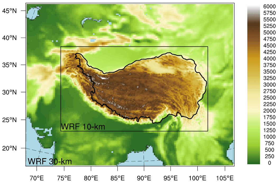
Figure 1 WRF domains and model topography (m). Solid black line in WRF 10 km domain represents the boundary of the TP.

2 Model and experimental setting

2.1 WRF model configuration

The WRF model version 4.0 was used in this study. The capability of spectral nudging towards water vapor mixing ratio was added in this version. A two-nested domain used in this study is displayed in Fig. 1. The outer domain with 30 km spatial resolution provides the large-scale information that has been resolved by the driving field. The inner domain with 10 km spatial resolution is the main study area and covers the complex terrain of the TP. The terrain of the region varies intensely in a short spatial range, which can exert strong turbulent drag on low-level atmospheric circulation and thus influence water vapor transport. To avoid the influence of regional difference when calculating the mean precipitation over the entire TP, evaluations of precipitation simulations were also conducted on extreme (i.e., the highest 5th percentile value) precipitation events.

The physical options used in this study followed the settings of the High Asia Refined (HAR) data (Maussion et al., 2011; Maussion et al., 2014). Specifically, the Thompson scheme (Thompson et al., 2004), the Grell 3D ensemble scheme (Kain, 2004), the Dudhia shortwave radiation scheme (Dudhia, 1989), Rapid Radiative Transfer model longwave radiation scheme (Mlawer et al., 1997), and the unified Noah Land Surface Model (Chen and Dudhia, 2001) were selected. The Yonsei University scheme (Hong et al., 2006) was used for the PBL scheme.

The initial and lateral boundary conditions were driven by the ERA-Interim reanalysis data (ERAI) with 6 h temporal and 79 km spatial resolution (Dee et al., 2011). The sea surface temperatures were also derived from ERAI. All seven simulations, including one without nudging and six with spectral nudging using various nudging strategies (Table 1), were initialized at 20 June 2008 and integrated continuously for 40 d with the first 10 d set to spin-up time. The total results for July 2008 are used for evaluation.

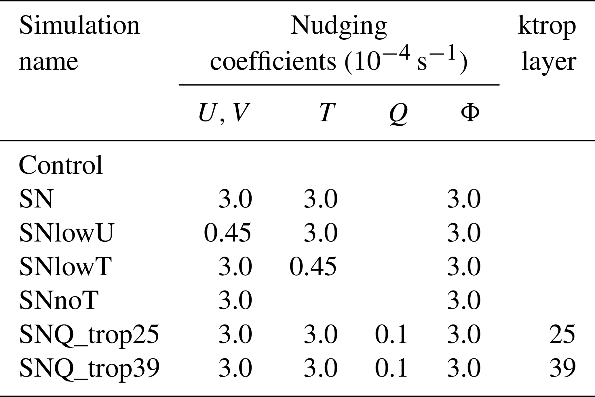
Table 1 Nudging coefficients (10⁻⁴ s⁻¹) used for spectral simulations. Spectral nudging is indicated by “SN”. U and V represent the horizontal wind component, T represents potential temperature, Q represents water vapor mixing ratio, and Φ represents geopotential. Nudging is applied to all layers above the PBL. Layer 39 represents approximately the mean pressure level of tropopause over the TP. Layer 25 represents approximately the normal lower limit for “ktrop” that is set to the middle layer in the model simulation.

2.2 Spectral nudging

Spectral nudging is used as a dynamical downscaling technique to retain all the large-scale information from the driving fields and to add smaller-scale information that the coarse driving fields cannot resolve. By adding a nudging term to the variable of model field, perturbation tendencies (differences between the regional field tendency and the driving field tendency) are dampened by spectral nudging at the selected spatial scale, and thus the inconsistency between model solution and the driving coarse field is alleviated. Following the study of Miguez-Macho et al. (2004), spectral nudging equation in WRF model is expressed as follows:

$$\begin{array}{}\text{(1)}& \begin{array}{rl}& {\displaystyle \frac{\text{d}Q}{\text{d}t}}=\\ & L\left(Q\right)-\sum _{\left|n\right|\le N}\sum _{\left|m\right|\le M}{K}_{mn}\left(Q_{mn}-Q_{omn}\right)e^{i{k}_{m}x}{e}^{i{k}_{n}y},\end{array}\end{array}$$

where Q is the prognostic variable to be nudged, L is the model operator, and Q_o is the variable from the driving fields. Q_mn and Q_omn represent the spectral coefficients of Q and Q_o, respectively. The nudging coefficient K_mn can vary with m and n (wave numbers in the x and y direction, respectively) and also with height; k_m and k_n imply the wave vector and depend on the domain size, D_x and D_y, which can be expressed as follows:

$$\begin{array}{}\text{(2)}& k_m={\displaystyle \frac{\mathrm{2}\mathit{\pi }m}{D_x}};k_n={\displaystyle \frac{\mathrm{2}\mathit{\pi }n}{D_y}}.\end{array}$$

In spectral nudging simulations, the cut-off wave number was set to a wavelength of 1000 km, and thus the nudging was applied only to the long waves whose physical wavelength was larger than 1000 km. This value of a wavelength has been validated to be the most appropriate nudging wavelength to simulate precipitation events (Gomez and Miguez-Macho, 2017; Yang et al., 2019). Therefore, the wave numbers of X and Y directions were 5 and 4, respectively, for the outer domain and 3 and 2, respectively, for the inner domain. Each nudging simulation was applied above the planetary boundary layer (PBL), allowing the near-surface small-scale processes to be free to respond to local processes (Lo et al., 2008).

2.3 Experimental settings

The conventional continuous integration without nudging was designated “control”. Default spectral nudging simulation was designated “SN”. The nudging coefficient is related to the nudging relaxation time, which indicates a predetermined timescale for how often nudging variables are relaxed toward the large-scale driving fields. In the SN simulation, nudging coefficients for horizontal wind, potential temperature, and geopotential on both domains were the default value of $\mathrm{3.0}\times {\mathrm{10}}^{-\mathrm{4}}$ s⁻¹ (relaxation timescale of 50 min). For water vapor mixing ratio, the default coefficient was $\mathrm{0.1}\times {\mathrm{10}}^{-\mathrm{4}}$ s⁻¹ (relaxation time scale of 24 h). An infinitely shorter relaxation time does not result in a higher consistency between the simulated small-scale fields with the forcing fields (Alexandru et al., 2009; Omrani et al., 2012). It is recommended to keep the relaxation time of nudging variables equivalent to the temporal interval of the input driving data (Omrani et al., 2013; Spero et al., 2018). Therefore, a nudging coefficient of $\mathrm{0.45}\times {\mathrm{10}}^{-\mathrm{4}}$ s⁻¹ (relaxation timescale of 6 h) was set for wind (SNlowU) and temperature (SNlowT) on the basis of SN to evaluate the sensitivity of model solution to nudging coefficient. Sensitivity simulation was not applied to geopotential because it has been shown to have a negligible influence when geopotential is nudged with different nudging coefficients (Spero et al., 2018).

A new option, “ktrop”, has been added in the released WRF model v4.0 that allows spectral nudging to be applied towards water vapor mixing ratio. This option adds a lid for both potential temperature and water vapor mixing ratio fields at a predefined layer (nominally selected to represent the tropopause) above the PBL, while the horizontal wind component and geopotential are not affected by the option.

As suggested from a 35-year analysis using ERAI, the pressure level of tropopause over the TP varies between 93 and 106 hPa, with a mean value of 100 hPa during summer (Zhou et al., 2019). Therefore, the associated level of tropopause was 39 (namely, ktrop = 39) in this study, and the relevant simulation was designated “SNQ_trop39”. Since the tropopause layer over the TP is much higher than other regions, it is necessary to examine the influence of adding the lid at a different model layer. The simulation in which the “ktrop” was set to the model layer of 25 was designated “SNQ_trop25”. The layer of 25 represented the index of the middle layer of the model in this study, which was the lower limit for “ktrop”. Considering the cold bias of atmospheric temperature in ERAI over the TP, the simulation with no nudging towards temperature at all was designated “SNnoT”, in which nudging towards moisture was not applied.

2.4 Validation data for model evaluation and comparison

Model-simulated precipitation was evaluated against the merged Climate Prediction Center (CPC) MORPHing technique precipitation dataset (hereinafter called CMORPH) with a temporal and spatial resolution of 1 h and 0.1^∘, which is developed by the China Meteorological Administration (CMA). The original CMORPH data, which have a spatial resolution of 8 km and temporal resolution of 30 min, are first resampled to the 0.1^∘ and 1 h spatial and temporal resolution. Following this, the systematic biases are corrected by 2400 rain gauges in China by using the probability density function matching method. The corrected CMORPH is subsequently combined with hourly rain gauge analysis from automatic stations to derive the merged hourly precipitation dataset by applying the optimal interpolation methods (Joyce et al., 2004; Xie et al., 2017). Many studies demonstrate the high consistency and acceptable bias of the CMORPH compared with the observed precipitation (Ou et al., 2020; Wei et al., 2018).

Beside the evaluation of precipitation, assessments of water vapor transport and large-scale atmospheric circulation are also particularly important, as they exert great influence during the formation of precipitation. Impacts of different spectral nudging strategies on the water vapor transport were compared with the ERAI and the fifth-generation global reanalysis of ECMWF, ERA5, which has a 31 km spatial resolution and 1 h temporal resolution. In this study, both ERAI and ERA5 were interpolated to the 10 km downscaled grid resolution as was done with the model output.

Figure 2 Spatial distribution of the mean and difference between, precipitation (mm d⁻¹) fields for July 2008. (a) CMORPH, (b) CMORPH precipitation smaller than P95 (5.73 mm d⁻¹), and (c) CMORPH precipitation larger than P95. Differences between CMORPH and (d) control, (e) SN, (f) SNlowU, (g) SNlowT, (h) SNnoT, (i) SNQ_trop25, and (j) SNQ_trop39. The bold solid black lines denote the boundary of the TP.

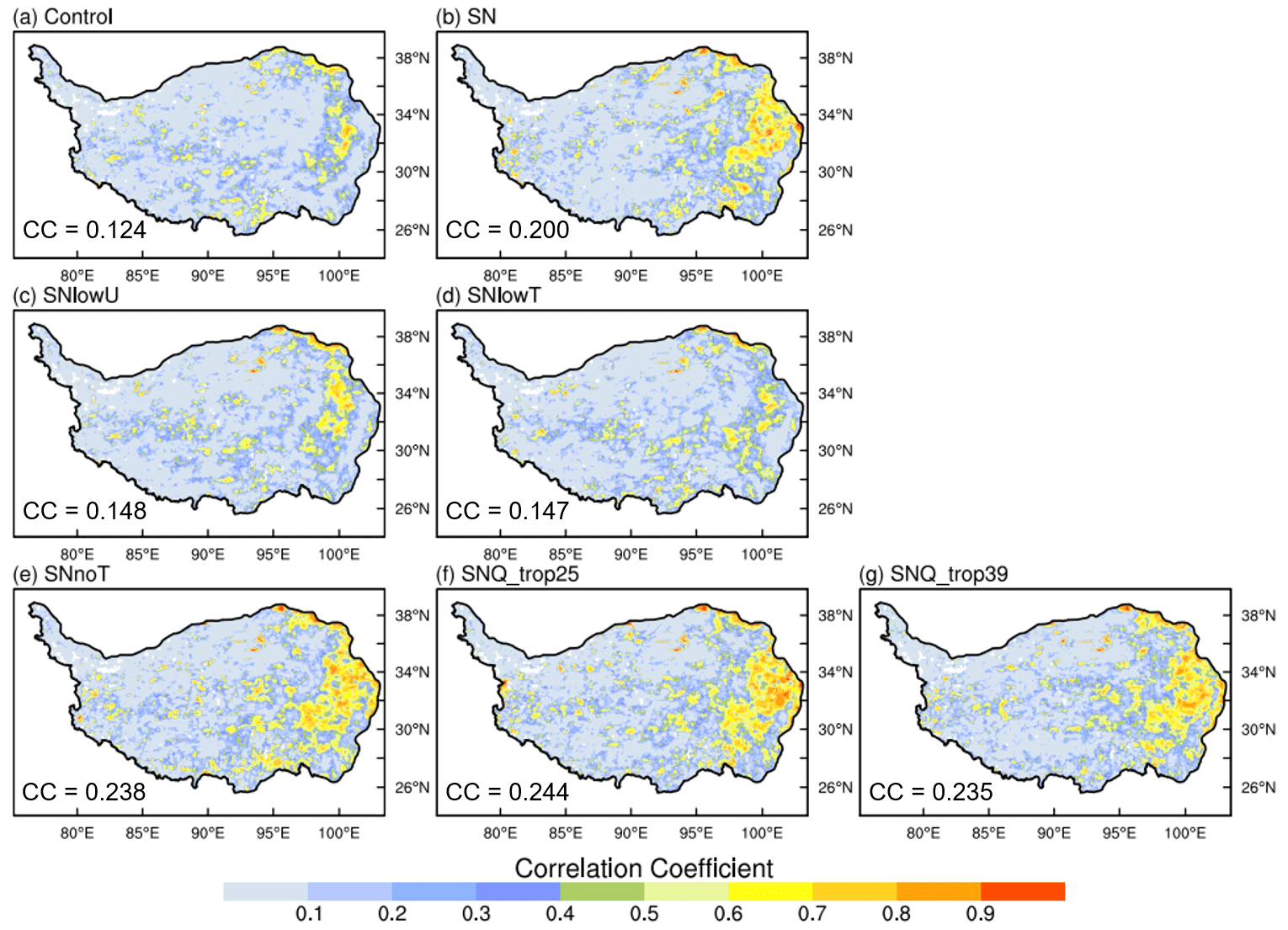
Figure 3 Spatial distribution of the temporal correlation between CMORPH and (a) control, (b) SN, (c) SNlowU, (d) SNlowT, (e) SNnoT, (f) SNQ_trop25, and (g) SNQ_trop39 over the TP.

Figure 4 (a) Root-mean-square error (RMSE) and (b) mean absolute error (MAE) of precipitation (mm d⁻¹) from WRF simulations against CMORPH at different precipitation thresholds (P95: monthly mean precipitation intensity at 5.73 mm d⁻¹). Color shading represents the performance of each WRF simulation, where more intense blue indicates a smaller bias in the simulation and more intense orange indicates a larger bias in the simulation.

3 Results

3.1 Impacts of nudging strategy on mean precipitation simulations

The spatial consistency between simulated results and CMORPH was investigated by the monthly mean (larger than 0.1 mm d⁻¹) and extreme (the highest 5 percentile value of) precipitation (P95, mm d⁻¹; equals to 5.73 mm d⁻¹ in this study). The monthly mean spatial distributions of the CMORPH precipitation fields of July and its difference with WRF simulations over the TP are depicted in Fig. 2. As shown in Fig. 2c, extreme precipitation can be observed over the southern and southeastern TP, and all simulations have large wet biases of precipitation compared to CMORPH, especially along the southern edge of the Himalayas.

The overestimation of precipitation over the eastern TP was reduced when using the spectral nudging method (Fig. 2e). However, both SNlowU and SNlowT experiments showed little improvement in alleviating the wet bias of precipitation simulation (Fig. 2f and g). Contrary to expectations, the SNQ_trop25 and SNQ_trop39 experiments (adding nudging towards the water vapor mixing ratio) produced the largest wet bias of all precipitation simulations, especially for extreme precipitation events over the southern TP (Fig. 2i and j). Although SNnoT did not fully eliminate the over-forecasting of precipitation, it showed the smallest wet bias of extreme precipitation events over the southern TP (Fig. 2h).

The spatial correlations were calculated from the time evolution of daily precipitation between CMORPH and simulations at each grid cell over the TP (Fig. 3). Overall, the correlation over the eastern TP in each experiment was found to be much higher than those over the western TP. Although model results have difficulties in capturing the temporal correlations with the CMORPH, some spectral nudging experiments significantly improved the correlation compared to the control simulation (Fig. 3e–g), in which the correlation coefficients simulated by SNnoT and SNQ experiments were larger than 0.6 over the eastern TP.

The validations of root-mean-square error (RMSE) and mean absolute error (MAE) on the monthly mean and extreme precipitation (P95) events were also conducted with CMORPH (Fig. 4). Color shading represents the performance of each simulation, where more intense blue indicates a smaller bias of simulation and more intense orange indicates a larger bias of simulation.

Consistent with aforementioned results, the RMSEs of some spectral nudging simulations were not always superior to the conventional continuous integration simulation. Note that SNlowT and SNlowU produced errors comparable to the control in terms of RMSE and MAE, whereas the default SN experiment performed worse for extreme precipitation events than the control experiments. Similar results were also found in the SNQ_trop25 and SNQ_trop39 experiments, where both experiments showed apparent higher RMSEs and MAEs compared to the control, up to 23.10 mm d⁻¹ (RMSE) in SNQ_trop39 for extreme precipitation events. The degraded skills of the SNQ_trop25 and SNQ_trop39 experiments in predicting precipitation were contrary to previous studies where adding spectral nudging toward water vapor mixing ratio could largely reduce the wet bias of precipitation intensity (Spero et al., 2014, 2018). In this assessment, the best performance was achieved by the SNnoT experiment with the lowest RMSE and MAE for different precipitation thresholds. It showed a clear advantage for the extreme precipitation event, reducing the RMSE by 1.16 mm d⁻¹ compared with the control and 2.27 mm d⁻¹ compared with the SN.

3.2 Evaluation of diurnal precipitation

In addition to error metrics, frequency distributions of precipitation intensity and diurnal cycle of the mean precipitation from WRF simulations were compared with CMORPH (Fig. 5). It is clear that precipitation from WRF simulations was heavily overestimated in the occurrence of precipitation events in which precipitation intensity exceeds 3 mm d⁻¹. With respect to the control and other spectral nudging strategies, the frequency distribution of precipitation intensity simulated by the SNnoT experiment was more comparable with CMORPH (Fig. 5a). The closer frequency density of the high-precipitation threshold indicated the advantage of restricting nudging for temperature and water vapor mixing ratio in the model may be attributed to decreasing the over-forecasting of extreme precipitation events over the southern TP.

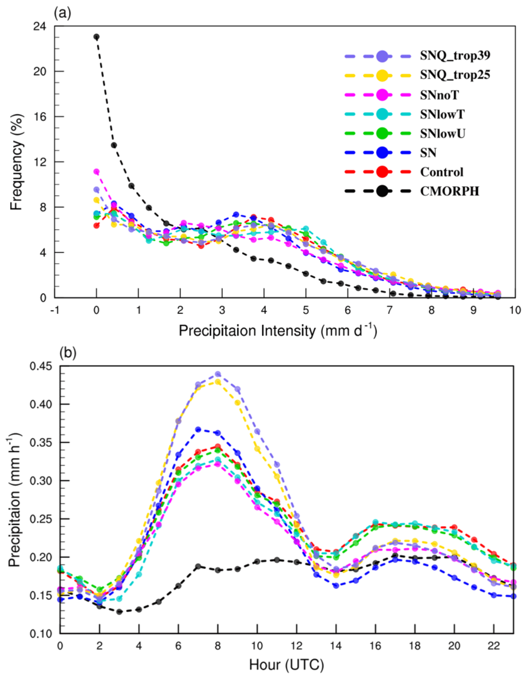
Figure 5 (a) The frequency distribution of mean precipitation intensity (mm d⁻¹) for CMORPH and simulated precipitation of July over the TP. (b) The average diurnal cycle of precipitation (mm h⁻¹) over the TP.

The diurnal cycle of precipitation is an important feature of the monsoon precipitation because it controls the circulation characteristic and affects the precipitation magnitude (Bhatt et al., 2014; Sato et al., 2008). To investigate whether using a spectral nudging method can improve the simulation of the diurnal cycle of precipitation, the variations in hourly precipitation from the CMORPH observations and model simulations are displayed in Fig. 5b. According to the CMORPH observations, the averaged peaks of hourly precipitation mainly occurred in the afternoon and at midnight local time (UTC+8) and reached 0.2 mm h⁻¹. The simulations of diurnal precipitation had comparable patterns to CMORPH but had a remarkably larger intensity during the day, indicating that some individual precipitation events may be misrepresented. Although the precipitation from SN showed an improvement in decreasing nighttime precipitation over-forecasts (the maximum of average precipitation was reduced by 0.05 mm h⁻¹), it performed worse than the control during the day. The precipitation intensity from the SNQ_trop39 and SNQ_trop25 experiments, however, had a much higher wet bias than the control, up to 0.1 mm h⁻¹, over the TP. The smallest wet bias of precipitation was found in the SNnoT experiment during the day, which also outperformed other experiments at night, reducing the over-forecast of precipitation by 0.03 mm h⁻¹ compared with the control and 0.05 mm h⁻¹ compared with the SN. Based on above analysis, precipitation forecasts during 02:00–12:00 UTC (10:00–20:00 LT) require urgent improvement in the model, even though the precipitation forecasts have been greatly improved by the SNnoT.

4 Discussion

4.1 Large-scale atmospheric circulation anomalies

In summer, precipitation occurred in the TP is mainly controlled by two water vapor channels, one of which is the transported by strong southwesterly under the effect of the Indian summer monsoon. The second channel is transported by the southern branch of the midlatitude westerly. Via the influence of both channels, a large amount of water vapor from the Bay of Bengal and the surrounding ocean could be transported to the TP (Xu et al., 2008, 2002; Zhou and Li, 2002).

The terrain of the Himalayas, featuring by a sharp topography gradient, is more than 5000 m in elevation on average and is regarded as a natural barrier for northward atmospheric flow. In summer, a large amount of atmospheric water vapor transport, originating from the surrounding oceans, impinges on the Himalayas. The sufficiently high topography strictly limits the upslope water vapor transport, and strong upward motions are consequently formed by the lifting effect of the complex terrain (Dong et al., 2016). However, the complex orography of the southern slope of the Himalayas is greatly smoothed in current RCMs. Accordingly, the surface friction and sub-grid orographic drag due to the impact of mesoscale and microscale orography on the airflow are weakened, which in turn reduce the convergence and condensation of water vapor over the southern slope of the Himalayas. Consequently, more water vapor transport could arrive the high-latitude TP, causing more precipitation over the TP.

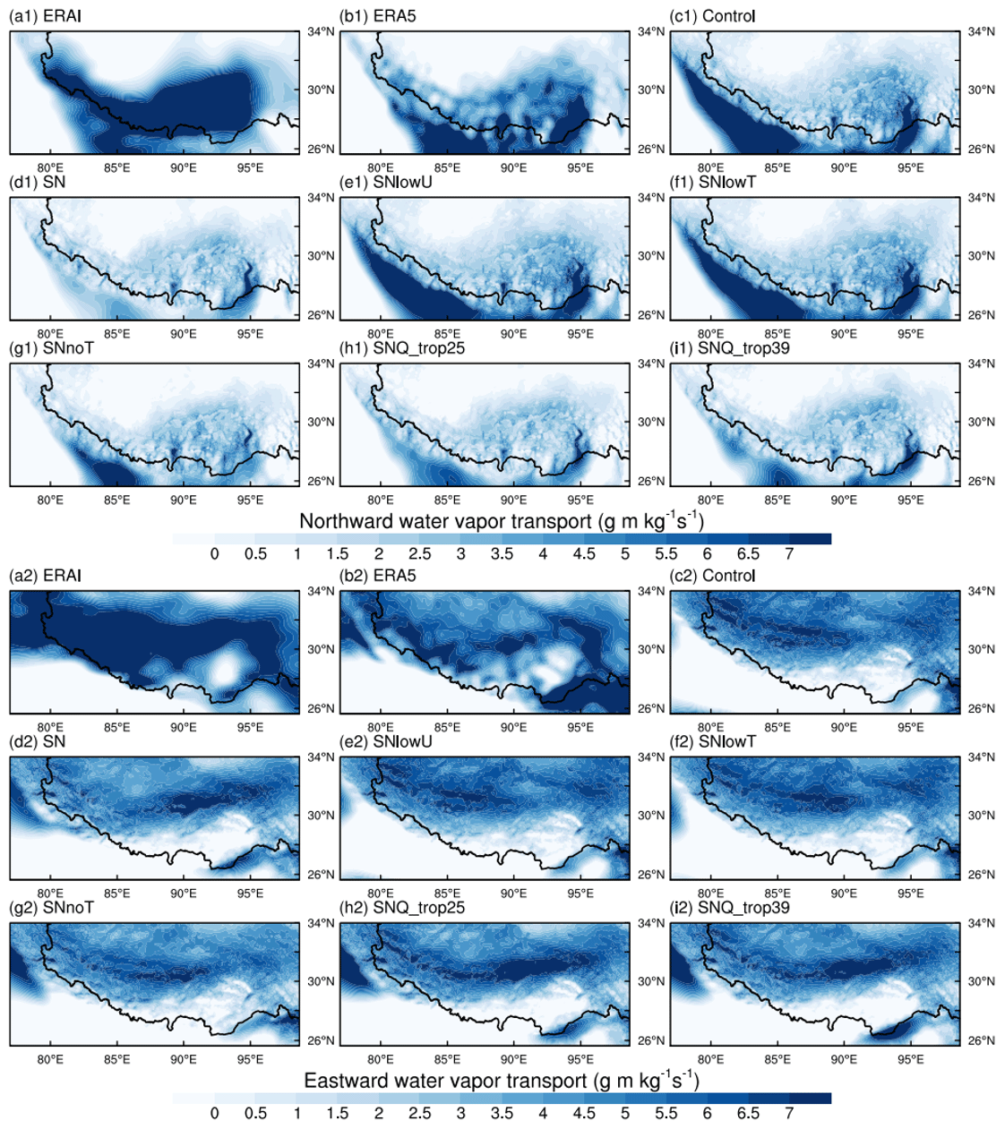
Figure 6 Column-integrated northward water vapor transport (meridional wind component multiples by specific humidity; g m kg⁻¹ s⁻¹) averaged over the study period over the central Himalayas derived from (a1) ERAI (ERA-Interim), (b1) ERA5, (c1) control, (d1) SN, (e1) SNlowU, (f1) SNlowT, (g1) SNnoT, (h1) SNQ_trop25, and (i1) SNQ_trop39. Panels (a2)–(i2) are the same as (a1)–(i1) but for the eastward water vapor transport (zonal wind component multiples by specific humidity; g m kg⁻¹ s⁻¹).

Column-integrated northward water vapor transport and eastward water vapor transport, averaged over the study period derived from ERAI, ERA5, and model simulations are displayed in Fig. 6. Large-scale atmospheric circulation forces strong water vapor transport into the southwestern TP, leading to a water vapor transport belt along the southwestern slope of the Himalayas. As represented by ERAI (Fig. 6a1 and a2), there was an obvious wet bias of water vapor transport over the TP and the central Himalaya. Although ERA5 showed a significant reduction in water vapor transport over the southern TP (Fig. 6b1 and b2); however, there was still excessive water vapor along the Himalayas, indicating that its coarse resolution was insufficient to resolve the impact of orographic drag on northward flow.

With higher spatial resolution and thus more detailed topography, all simulations reproduced such atmospheric water vapor fields over the southern TP but with weaker magnitude compared to ERAI and ERA5. Note that not all spectral nudging experiments retained the large-scale character of water vapor transport. From Fig. 6d1, SN simulated an anomalous weak northward water vapor transport over the western Himalayas, where SN misrepresented the large-scale information that has been resolved by the global reanalysis data assimilation (EARI and ERA5). Although SNlowU and SNlowT (Fig. 6e1 and f1) showed comparable results with those of the control (Fig. 6c1), eastward water vapor transport of SNlowU and SNlowT were slightly weaker than control over the western TP (Fig. 6e2 and f2). SNQ_trop25 and SNQ_trop39 (Fig. 6h1 and i1) simulations with nudging toward moisture showed an analogous northward water vapor transport over the Bay of Bengal, indicating that the difference between SNQ_trop25 and SNQ_trop39 in precipitation simulations may be attributed to local convection and subsequently processes. With reference to the above, water vapor transport obtained by SNnoT (Fig. 6g1 and g2) showed the most significant reduction over the TP compared to the other spectral nudging experiments. As anticipated from the precipitation anomalies, such a decrease in water vapor transport of SNnoT is obviously related to the smaller wet bias of precipitation.

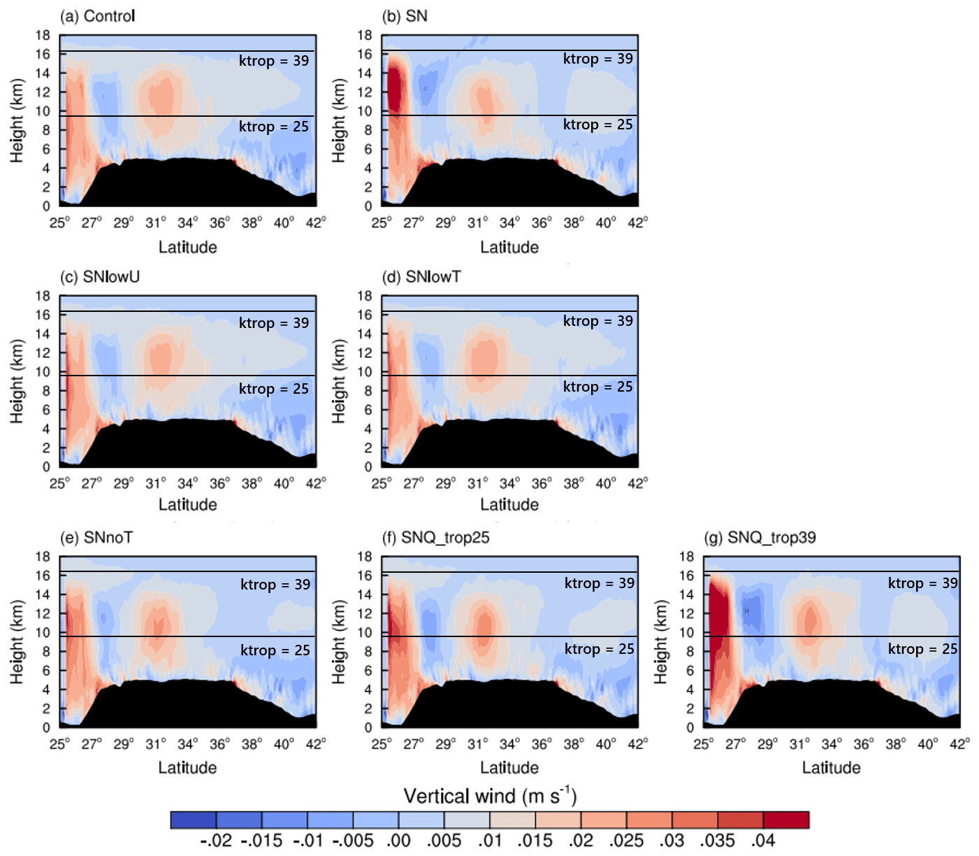
Figure 7 Vertical wind (m s⁻¹; a positive value means upward wind, and a negative value means downward wind) along the average of the 85–95^∘ E cross section for the following simulations: (a) control, (b) SN, (c) SNlowU, (d) SNlowT, (e) SNnoT, (f) SNQ_trop25, and (g) SNQ_trop39. Solid black lines represent the height of the “ktrop” layers 25 and 39.

Figure 8 The same as Fig. 7 but along the average fields of 26–34^∘ N.

4.2 Vertical structure of the convective process

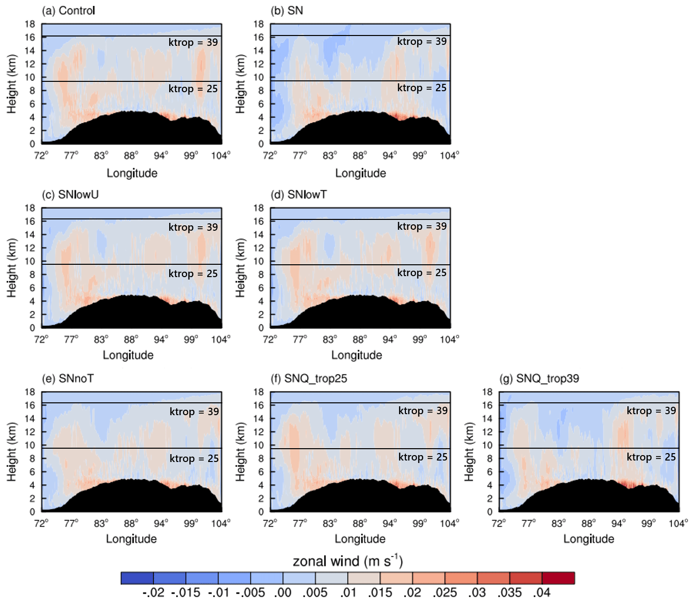
The TP and its surrounding area have been regarded as a favorable region for convective processes because of its strong topography gradient. Deep convection favors the process of transporting water vapor into the upper-level atmosphere, through which moisture flux can be vertically released into the atmosphere and influences the formation of precipitation during the summer monsoon season (Fu et al., 2006; Heath and Fuelberg, 2014). Figures 7 and 8 illustrated the monthly mean cross section of vertical wind along the averaged fields of 85–95^∘ E and 26–34^∘ N from seven experiments, respectively. In order to clearly distinguish the impact of restricting nudging of temperature and moisture, solid black lines that represent the height of “ktrop” layer 25 (near the height of 9.6 km) and 39 (near the height of 16.1 km) were plotted in Figs. 7 and 8.

Because the horizontal and vertical variations in moisture and temperature at the upper troposphere have not been sufficiently resolved by global driving datasets (Miguez-Macho et al., 2004), the lid was originally designed to avoid transferring moisture and temperature biases above the tropopause in the reference field to the model-simulated field. The strongest upward motion along the latitude was simulated by SNQ_trop39 (Fig. 7g) over the southern slope of the Himalayas, followed by the SN and SNQ_trop25 (Fig. 7b and f). In the two SNQ simulations, the upward motion was obviously decreased when the lid was applied at the lower model level (Fig. 7f and g). From above comparison, it is clear that nudging towards temperature and moisture at the middle troposphere was likely to enhance the atmospheric upward motion over the southern slope of the Himalayas. Therefore, more water vapor could be transferred to the upper troposphere and was subsequently transported to the interior of the TP through high-level southwestern atmospheric advection, causing more precipitation over the TP.

In this case, nudging towards temperature and moisture was restricted in the entire model layer, assuming that nudging towards horizontal wind components and geopotential height was strong enough to reduce large-scale errors in the wave component of temperature and moisture. As shown in Fig. 7e, a clear reduction in the magnitude of upward motion over the southern slope of the Himalayas was simulated by SNnoT, and a similar result was also observed in Fig. 8e. Therefore, the upslope water vapor transport was strictly limited by the sufficiently high Himalayas and was condensed during upslope flow, causing there to be little water vapor available for precipitation over the interior of the TP. With reference to the above analysis, the lid at the tropopause layer in the model is inappropriate when simulating precipitation over the TP.

4.3 Vertical profile of horizontal wind components, atmospheric temperature, and specific humidity

The spectral nudging technique is supposed to alleviate the inconsistence between the regional model field and the driving field (e.g. ERA-Interim). However, previous studies of WRF simulations centered over the TP that used ERA-Interim reanalysis as the driving fields have a large bias in the water vapor transport over the TP (He et al., 2019; Xu et al., 2017). Therefore, the reason why we do not nudge towards temperature and moisture at all is to prevent external forcing of moisture and temperature (from nudging) so that their small-scale dynamical features are not affected. In order to show how the settings of nudging parameters influenced the consistency of nudged variables between the model field and the driving field, vertical profiles of nudged variables averaged over the TP for the study period were calculated. The difference between ERA-Interim (ERAI) and seven WRF simulations at each pressure layer is displayed in Fig. 9, and relevant statistical error metrics are given in Table 2.

Table 2 Statistical error metrics (MB: mean bias; RMSE: root-mean-square error) of the column-averaged zonal wind component (U; m s⁻¹), meridional wind component (V; m s⁻¹), atmospheric temperature (K), and specific humidity (kg kg⁻¹) derived from seven WRF simulations versus ERA-Interim (ERAI) over the TP for the study period.

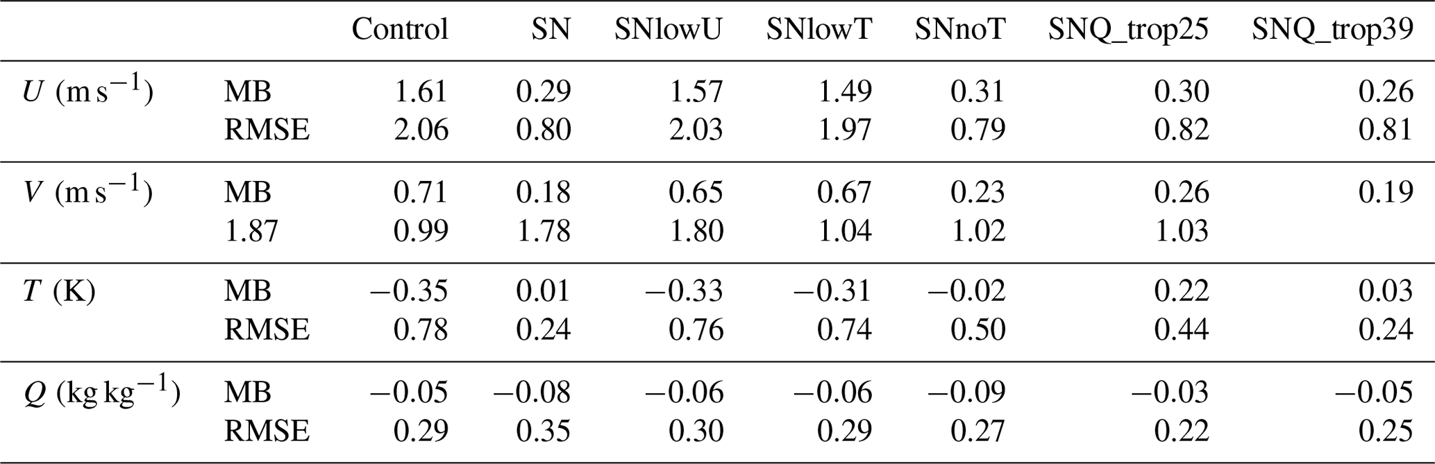
Compared to the control simulation, obvious improvements are observed in both eastward and northward wind components when spectral nudging was applied (Fig. 9a and b). Specifically, most of simulations with spectral nudging showed comparable eastward wind speed with ERAI in the each pressure layer, and reduced the bias of eastward wind speeds by 1.2 m s⁻¹ compared to the control (Table 2). Similarly, although all simulations produced stronger northward wind speeds than ERAI, the use of spectral nudging reduced the bias by 0.8 m s⁻¹ against the control simulation (Table 2). In terms of SNnoT (purple line), its consistency in both the zonal and meridional wind fields was not affected by the influence of restricting nudging towards temperature and moisture, with the RMSE of 0.79 m s⁻¹ of U and RMSE of 1.04 m s⁻¹ of V. However, both SNlowU and SNlowT simulations, which had decreased nudging coefficient for winds and temperature, had similar patterns to the control simulation in terms of horizontal wind speeds and atmospheric temperature (Fig. 9c). One possible reason could be their weaker nudging coefficient (0.000045 s⁻¹), indicating that the horizontal wind component and the temperature of the model field were relaxed for the driving field at every 6 h, which is equal to the input time interval of ERAI. It may weaken the impact of applying spectral nudging on the nudged variables and thus simulate similar temperature and horizontal winds to the control.

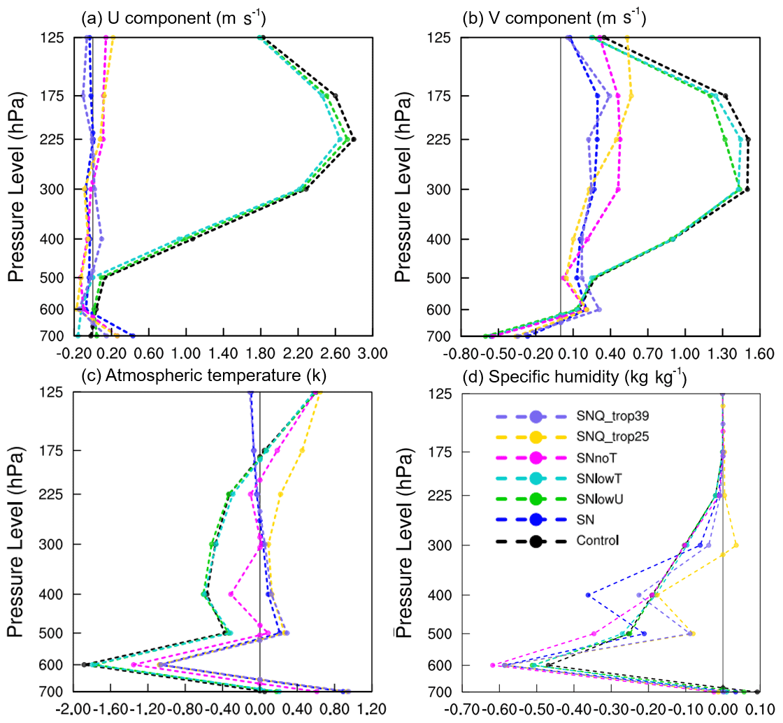
Figure 9 Vertical profile of difference fields between ERA-Interim and seven WRF simulations averaged over the study period for the (a) zonal wind component (U; m s⁻¹), (b) meridional wind component (V; m s⁻¹), (c) atmospheric temperature (K), and (d) specific humidity (kg kg⁻¹) over the TP. The vertical solid gray line represents the value of 0.0 at each pressure layer.

An apparent improvement was observed in the spectral nudging experiments in that they reduced the cold bias compared to the control (Fig. 9c). Although the performances of SNlowU and SNlowT were highly comparable to the control, both SNlowU and SNlowT simulated higher temperatures at lower levels and had slightly lower RMSEs. The discrepancy between SN, SNQ_trop25, and SNQ_trop39 in terms of temperature field was found in the pressure layer higher than 300 hPa, where the temperature in SNQ_trop25 was higher than SN and SNQ_trop39. The higher temperature of SNQ_trop25 was likely attributed to its higher water vapor within the free troposphere (Fig. 9d), which caused wetter atmosphere conditions; thus, more heat flux was released once precipitation began. The vertical profile of temperature in SNnoT was aligned with the SNQ_trop25 in the upper troposphere but had smaller temperature. These comparisons indicated that limiting nudging towards temperature in model produced higher temperature.

Considering the wet bias of water vapor of ERAI over the TP, the best performance in reducing the wet bias of the water vapor was achieved by the SNnoT, despite the SN simulating slightly drier water vapor, with a value of 0.17 k kg⁻¹ at 400 hPa. Both SNQ_trop25 and SNQ_trop39 simulated the wettest atmospheric water vapor content, but SNQ_trop25 had higher water vapor than SNQ_trop39 when spectral nudging towards the water vapor mixing ratio was limited above 300 hPa in the SNQ_trop25 experiment. Based on above results, spectral nudging towards water vapor mixing ratio in more atmospheric layers will reduce the wet bias of water vapor. However, such a reduction in simulated atmospheric water vapor could not compensate for the wet bias of the driving field (ERAI) that has been artificially introduced by applying spectral nudging towards water vapor. Moreover, according to the study of He et al. (2019), atmospheric temperature in ERA-Interim against sounding observations showed an apparent cold bias when the pressure layer was higher than 400 hPa over the TP.

In summary, the inter-comparisons of the ensemble model simulations demonstrated that SNnoT achieved notable improvements over the control and the remaining spectral nudging experiments. It not only improved the agreement of model wind filed with ERAI but also reduced the cold bias of temperature above 400 hPa and the wet bias of moisture within troposphere over the TP. The weakened upward motion over the southern slope of the Himalayas and the weakened water vapor transport simulated by the SNnoT limited the water vapor to be transported to the interior of the TP, leading to less moisture being available for precipitation. The improved moisture transport and large-scale circulation will have significant implications for precipitation analysis and water cycle budgets over the TP.

5 Conclusions

In the case of downscaling the coarse-resolution reanalysis, regional climate simulations suffer from the large-scale errors due to the inconsistencies between the model solution and the driving field along the boundaries because of the systematic error of RCM (Miguez-Macho et al., 2004; Waldron et al., 1996). The spectral nudging technique is thus used to relax the specific spectral scale of variables in model field towards the driving field, in order to alleviate the inconsistencies. In this paper, a set of simulations was evaluated to reveal the influence of applying the spectral nudging technique in the WRF model for simulating precipitation and associated nudged variables over the TP.

Firstly, evaluations against the CMORPH precipitation data indicated that conventional continuous simulation cannot reproduce actual precipitation patterns and largely overestimate precipitation events over the western and northern TP. The use of spectral nudging in the WRF model reduced such overestimations but did not always overcome all deficiencies when simulating the precipitation intensity and its diurnal cycle. Spectral nudging experiments with decreased nudging coefficients ($\mathrm{4.5}\times {\mathrm{10}}^{-\mathrm{5}}$ s⁻¹) for wind and potential temperature showed comparable results with conventional continuous simulation in terms of horizontal wind components and temperature simulations. In addition, allowing spectral nudging towards water vapor mixing ratio in more atmospheric layers within the troposphere can reduce the wet bias of water vapor. But this improvement cannot compensate for the wet bias of the driving field (ERAI) that has been artificially introduced by applying spectral nudging towards water vapor. Therefore, although the ERA-Interim reanalysis has been widely used as the large-scale driving field for regional climate studies centered the TP in RCMs, the cold bias of atmospheric temperature and wet bias of water vapor over this region should be strongly considered in the case of downscaling the ERA-Interim reanalysis.

To decrease the influence of the biases in precipitation simulation, spectral nudging towards potential temperature and the water vapor mixing ratio was restricted in the whole layers, preventing the external forces on moisture and temperature (from nudging) to affect small-scale dynamics. The change to spectral nudging had clear advantages over conventional continuous simulation and other spectral nudging experiments, and largely improved the simulation of precipitation intensity and its diurnal cycle over the TP. Based on subsequent analysis, SNnoT reduced the meridional water vapor transport and upward motion at the southern slope of the Himalayas; thus, less water vapor could reach the upper troposphere, causing less precipitation over the southern TP. Consistently, SNnoT also improved the simulations of atmospheric temperature and the water vapor mixing ratio by collectively alleviating the cold bias of temperature and wet bias of the water vapor.

The evaluation and improvement of the spectral nudging technique in the WRF model in this work not only concentrates on optimizing precipitation forecasts but also aims to increase the reliability of RCM data used to assess the regional climate change without degrading the simulations of temperature and water vapor. The conclusion of this work is also useful for the application of RCMs in dynamical downscaling processes when using different reference fields. Since regional cumulus and land surface processes are also essential in regional climate modeling because of their significant effects on both large-scale and regional atmospheric circulation, improvements in representing such physical processes are required in future studies.