the Creative Commons Attribution 4.0 License.
the Creative Commons Attribution 4.0 License.
 | 10 May 2021
Ecosystem age-class dynamics and distribution in the LPJ-wsl v2.0 global ecosystem model
Benjamin Poulter
Forest ecosystem processes follow classic responses with age, peaking production around canopy closure and declining thereafter. Although age dynamics might be more dominant in certain regions over others, demographic effects on net primary production (NPP) and heterotrophic respiration (Rh) are bound to exist. Yet, explicit representation of ecosystem demography is notably absent in many global ecosystem models. This is concerning because the global community relies on these models to regularly update our collective understanding of the global carbon cycle. This paper aims to present the technical developments of a computationally efficient approach for representing age-class dynamics within a global ecosystem model, the Lund–Potsdam–Jena – Wald, Schnee, Landschaft version 2.0 (LPJ-wsl v2.0) dynamic global vegetation model and to determine if explicit representation of demography influenced ecosystem stocks and fluxes at global scales or at the level of a grid cell. The modeled age classes are initially created by simulated fire and prescribed wood harvesting or abandonment of managed land, otherwise aging naturally until an additional disturbance is simulated or prescribed. In this paper, we show that the age module can capture classic demographic patterns in stem density and tree height compared to inventory data, and that simulated patterns of ecosystem function follow classic responses with age. We also present two scientific applications of the model to assess the modeled age-class distribution over time and to determine the demographic effect on ecosystem fluxes relative to climate. Simulations show that, between 1860 and 2016, zonal age distribution on Earth was driven predominately by fire, causing a 45- to 60-year difference in ages between older boreal (50–90∘ N) and younger tropical (23∘ S–23∘ N) ecosystems. Between simulation years 1860 and 2016, land-use change and land management were responsible for a decrease in zonal age by −6 years in boreal and by −21 years in both temperate (23–50∘ N) and tropical latitudes, with the anthropogenic effect on zonal age distribution increasing over time. A statistical model helped to reduce LPJ-wsl v2.0 complexity by predicting per-grid-cell annual NPP and Rh fluxes by three terms: precipitation, temperature, and age class; at global scales, R2 was between 0.95 and 0.98. As determined by the statistical model, the demographic effect on ecosystem function was often less than 0.10 kg C m−2 yr−1 but as high as 0.60 kg C m−2 yr−1 where the effect was greatest. In the eastern forests of North America, the simulated demographic effect was of similar magnitude, or greater than, the effects of climate; simulated demographic effects were similarly important in large regions of every vegetated continent. Simulated spatial datasets are provided for global ecosystem ages and the estimated coefficients for effects of precipitation, temperature and demography on ecosystem function. The discussion focuses on our finding of an increasing role of demography in the global carbon cycle, the effect of demography on relaxation times (resilience) following a disturbance event and its implications at global scales, and a finding of a 40 Pg C increase in biomass turnover when including age dynamics at global scales. Whereas time is the only mechanism that increases ecosystem age, any additional disturbance not explicitly modeled will decrease age. The LPJ-wsl v2.0 age module represents another step forward towards understanding the role of demography in global ecosystems.
- Article
(7936 KB) - Full-text XML
-
Supplement
(1369 KB) - BibTeX
- EndNote


Forest ecosystem production follows predictable patterns with time since disturbance. Classic forest age–production curves from Odum (1969) suggest that net ecosystem production (NEP) peaks around canopy closure, declining thereafter due to hydraulic limitations on gross primary production (GPP) (Ryan et al., 2004; Drake et al., 2010, 2011) and increases in heterotrophic respiration from biomass turnover due stand-level declines in population density (Pretzsch and Biber, 2005; Stephenson et al., 2014). That younger forests are more productive than older forests has been long-standing knowledge in forestry, as evidenced by yield and growth tables dating back to the 18th century that incorporated stand age into their calculations of lumber production (Pretzsch et al., 2008).
On global scales, forest age is a considerable factor in the global carbon cycle and comprises a large fraction of the total land carbon sink, which is estimated at 3.2±0.8 Pg C yr−1 for the years 2008–2017 (Le Quéré et al., 2018). According to country-level forest inventories, net carbon uptake from post-disturbance tropical forest regrowth was 1.6±0.5 Pg C yr−1 from 1990 to 2007 (Pan et al., 2011a). Although the timeframes for estimates of the total land sink and the inventory-based regrowth flux do not perfectly overlap, the magnitude of the regrowth sink relative to the total land sink warrants that models take regrowth dynamics into account. A multi-model global regrowth analysis with demographically enabled dynamic global vegetation models (DGVMs), to which Lund–Potsdam–Jena – Wald, Schnee, Landschaft version 2.0 (LPJ-wsl v2.0) contributed, estimated that post-disturbance regrowth comprised a large global regrowth sink of 0.3 to 1.1 Pg C yr−1 due to demography alone over the years 1981–2010 (Pugh et al., 2019b). In the last decade, explicit model representation of forests as a function of time since disturbance (hereafter simply, “ecosystem age”) has been a grand challenge in an effort to quantify the demographic response of forests to changes in climate, atmospheric CO2, land-use change and land management (LUCLM), and fire (Friend et al., 2014; Kondo et al., 2018; Pugh et al., 2019b). Much of the focus of these global modeling studies has been on the effect of natural and anthropogenic disturbances on the carbon dynamics in old-growth versus second-growth forests (Gitz and Ciais, 2003; Shevliakova et al., 2009; Kondo et al., 2018; Yue et al., 2018; Pugh et al., 2019b) but lack finer distinction of demographic effects at different age classes. Following a call to the science community to improve demographic representation in models (Fisher et al., 2016), there is now a growing list of global models that are capable of simulating global ecosystem demographics (Gitz and Ciais, 2003, OSCAR; Shevliakova et al., 2009, LM3V; Haverd et al., 2014, CABLE-POP; Lindeskog et al., 2013, LPJ-GUESS; Yue et al., 2018, ORCHIDEE MICT; Nabel et al., 2020, Jena Scheme for Biosphere Atmosphere Coupling in Hamburg version 4 – JSBACH4), although more models need the capability to represent landscape heterogeneity in forest structure and function.
Much of the evidence for the relative importance and global distribution of large disturbances has come from either satellite retrievals of spectral indices indicating forest loss or burn scars on the land (Potter et al., 2003; Frolking et al., 2009; Pugh et al., 2019a), national forest inventory records of land-use change and forest management (Houghton, 1999; FAO-FRA, 2015; Williams et al., 2016), or model-based studies (Goldewijk, 2001; Arneth et al., 2017) that integrate information on historical land use (Goldewijk, 2001; Hurtt et al., 2006). Other natural disturbances such as pest and pathogen outbreaks, flooding, ice storms, and volcanic eruptions are less widespread globally (Frolking et al., 2009) but are still influential drivers of landscape age-class dynamics (Dale et al., 2001; Turner, 2010). In the conterminous United States, forest management is the predominant forest disturbance (1.4 % of forested area converted to non-forest and then re-established annually), followed by fire (0.01 %–0.5 % of forested area burned annually 1997–2008) (Williams et al., 2016). Although pests and pathogens, namely bark beetle infestations, affected a much larger area (up to 6 % of total forested area in the US) than both logging and fire, their effects do not always cause immediate tree mortality. It is arguable whether fire and LUCLM are the two most important global drivers of ecosystem age (Pan et al., 2011a), but nevertheless these are the drivers applied in a model framework in this study, in a manner that moves modeling one step forward to assess global age-class dynamics.
The overall aims of this study are to present new model developments that simulate the time evolution of age-class distributions in a global ecosystem model and to determine if explicit representation of demography in this model influenced ecosystem stocks and fluxes at global scales or at the level of a grid cell. Technical details are presented for a module representing age-class dynamics, driven by fire feedbacks, land abandonment, and wood harvesting in the LPJ-wsl v2.0 DGVM. Prior versions of LPJ-wsl v2.0 that included early developments of the land-use change module and the age-class module have already contributed to previous studies (Arneth et al., 2017; Kondo et al., 2018; Pugh et al., 2019b). Analyses of model behavior, in terms of age–structure and age–functional patterns, the temporal evolution of age distributions and their causative drivers, and a statistical model of ecosystem production and respiration as a function of demography and climate, are presented.
2.1 LPJ-wsl v2.0 general model description
2.1.1 LPJ history
LPJ-wsl v2.0 has its legacy in the LPJ family of models, first developed by Sitch et al. (2003) in a Fortran coding environment1. In 2007, Bondeau et al. (2007) produced the LPJ managed Land (LPJmL) codebase, in C, which included the addition of “managed lands”. The model known as LPJ-wsl v2.0 is based on LPJmL v3.0 but includes modifications to managed lands that now includes modeling gross land-cover transitions, forest age cohorts, and also a modification that include permafrost and wetland methane; the permafrost and wetland modules were not used in this study. Many developments were made in the publicly available LPJmL4 (version 4.0; Schaphoff et al., 2018) that are not present in LPJ-wsl v2.0. The LPJ-wsl v2.0 model was branched off of LPJmL some time around 2010 and continued to diverge. This research paper represents a large effort toward this end, and the LPJ-wsl v2.0 code is now freely and publicly available (https://github.com/benpoulter/LPJ-wsl_v2.0, last access: 28 July 2020) under GNU Affero General Public License version 3.

Figure 1LPJ-wsl v2.0 model structure of inputs (red), time steps (blue), and the level at which state variables are tracked within grid cells and sub-grid-cell age classes (green), such as age classes or land uses. Simulation of abiotic, biotic, and ecological processes occurs at the scale of an age class.
2.1.2 LPJ-wsl v2.0 overview
LPJ-wsl v2.0 simulates soil hydrology and vegetation dynamics in 0.5∘ grid cells, wherein climate, atmospheric CO2, and soil texture are prescribed from driver datasets (Fig. 1). Vegetation is categorized into plant functional types (PFTs; Box, 1996). Plant populations compete for light, space, and soil water, depending on demand; nutrient cycles are not considered in this model version. LPJ-wsl v2.0 is a “big-leaf” ecosystem model, whereby leaf-level photosynthesis and respiration (Haxeltine and Prentice, 1996; Farquhar et al., 1980) occur at daily time steps, accounting for the photosynthetically active period (daytime), and are scaled to the stand level using a mean-individual approximation, which assumes that important state variables (carbon stocks and fluxes) can be determined by using the average properties of a population. Plant populations are categorized using 10 PFTs in this study (phenology parameters and bioclimatic limits listed in Table S1), which are the same PFTs as in Sitch et al. (2003). Left unchanged are the PFT-specific bioclimatic limits, turnover rates, C:N tissue ratios, allometric ratios, and other parameters not explicitly commented on here but as described in Sitch et al. (2003). Mortality occurs as in the original version of LPJ, “… as a result of light competition, low growth efficiency, a negative annual carbon balance, heat stress, or when PFT bioclimatic limits are exceeded for a period of time” (Sitch et al., 2003). The fire module and the representation of land-use change and land management are described in detail in Sect. 2.2.2, as these modules require a greater number of modifications for integration with age classes.
2.2 Age-class module
2.2.1 An age-based model of ecosystems – sub-grid-cell dynamics
Age classes are represented as “patches” within a grid cell (Fig. 1). Every age class has the same climate, atmospheric CO2, and soil texture, but the properties of the age class, such as available soil water and light availability, are determined by feedbacks from plant demand within an age class. Plant processes (competition, photosynthesis, respiration) are simulated at the level of the age class for each PFT within the age class.
Table 1Age-class widths corresponding to two different simulation age-class setups in LPJ-wsl v2.0. The age-class codes are referenced in figures.
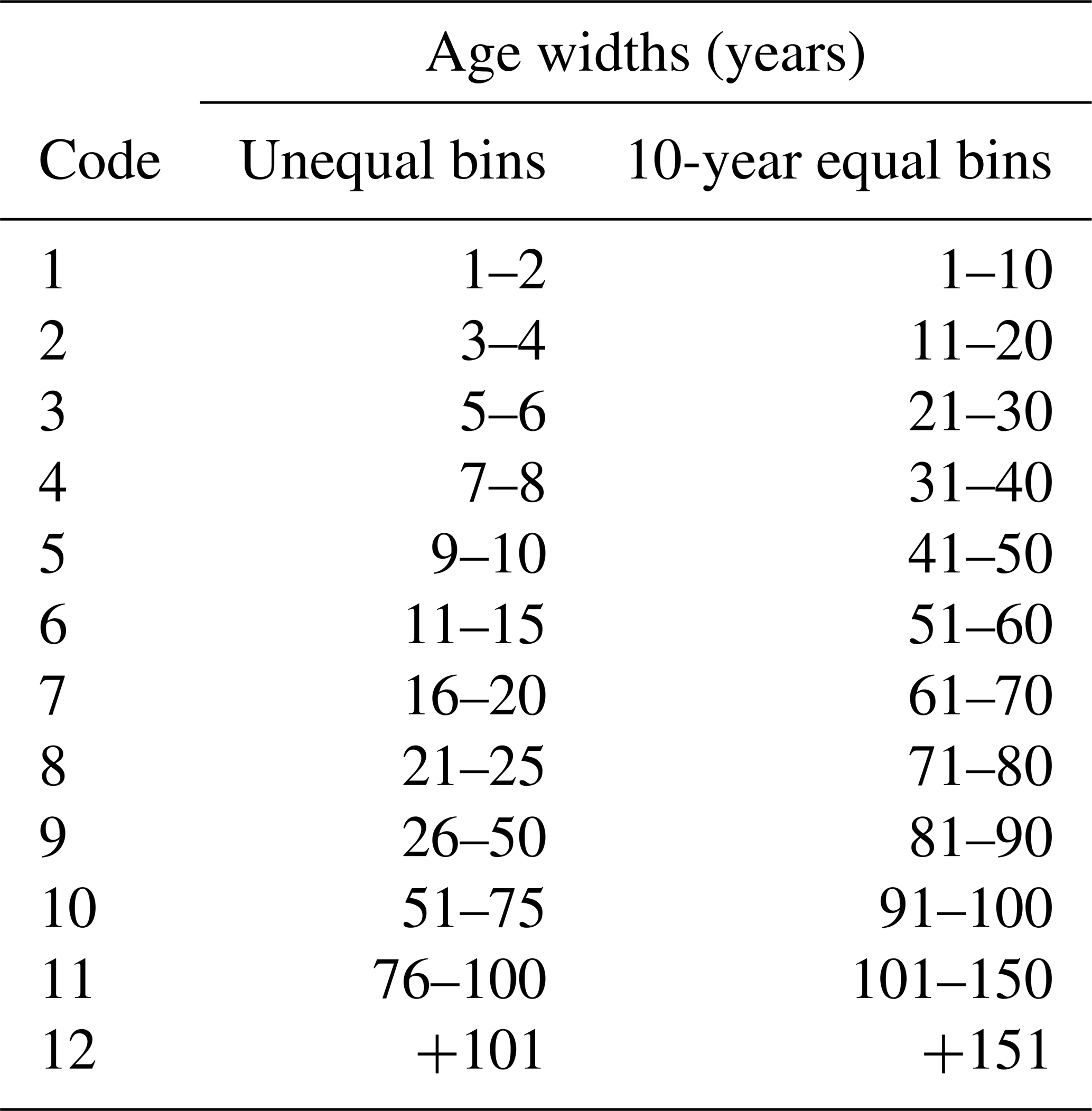
The age-class module has a fixed number of age classes that can be represented in a grid cell, but all age classes are not always represented. Age classes are classified into 12 age classes in fixed age-width bins, defined as the unequalbin or the 10yr-equalbin age-width setup (Table 1). Each age class contains within-age-class elements, which are simply a vector representation of areas for each age unit in the age class. The within-age-class elements are not independent, and every within-age-class element has the same state variables, including the same soil water and light. As such, we only simulate processes at the age-class level, and the within-age-class elements are a simple method for a “smooth” transition between age classes. In theory, we can simulate processes independently for each within-age-class element, but this is not practical or necessary. The main benefit for using equal-bin or unequal-bin age classes is to independently simulate processes. The age widths of the age classes in the 10yr-equalbin setup correspond to common age widths of classes used in forest inventories; for contrast, JSBACH4 uses a 15-year age width in their equal-bin age-class setup. Most age classes in this setup are represented by a vector of 10 elements, wherein each element represents an aerial fraction for each age unit (Table 1). The 10yr-equalbin age setup is used for all simulations including the global simulation, whereas the unequalbin setup is used for regional and single-grid-cell simulations; simulation details are in next section. The use of equal or unequal age-class setups is more than just for reporting purposes. Resources available to plants (space, light, soil water) differ between age classes but not within age classes, and we limit the model to represent a total of 12 age classes only. Also, there exists a greater range of forest ages at global scales and the equal-bin age-class setup allows us to independently model resource dynamics for more of the terrestrial surface. If we had chosen the unequal-bin setup for global simulations, we would be independently modeling processes only for the youngest age classes and we would lose capacity to independently model processes at intermediate and older age classes. A study by Nabel et al. (2020), using the demographically enabled JSBACH4 DGVM, found that unequal binning of age widths had lower errors than equal-age-width binning but the largest reduction in model–observation error was achieved by simply adding more age classes at younger ages, regardless of the binning strategy employed.
Age classes are only created by disturbance, and we only model the following disturbances: fire, wood harvest, or land abandonment, which initialize a new, youngest age class. The fraction of the age class that burns gets its age “reset” to the youngest age class (1–10 years). The same process occurs for the fractional area that undergoes wood harvest or when managed land is abandoned and allowed to regrow – the fractional area undergoing an age transition is reclassified as a 1- to 10-year age class. This process allows the model to accurately track the carbon stocks, fluxes, and feedbacks associated with these state variables. For example, if a fire burns 50 % of an age class, then 50 % might have bare ground and 50 % will have vegetation at pre-burn levels. If the probability of another fire is dependent on live vegetation, then feedbacks will result in a lower chance of fire on the bare-ground fraction versus the fully vegetated fraction that was not previously burned.
The most novel advancement in this study is a new method of age-class transition modeling, which we call “vector tracking of fractional transitions” (VTFT), which improves the computational efficiency of modeling age classes in global models; there is a similar approach independently conceived by Nabel et al. (2020). The method is a transparent and simple solution to the problem of dilution, which manifests as an advective process when state variables, such as carbon stocks or tree density, are made to merge by area-weighted averaging. The concept of merging two unique age classes on the basis of similarity is a computational solution to constrain the number of simulated age classes in accordance with computer resources but can be considered ecologically unrealistic. For example, along what axis of similarity is an age class considered to be most similar to another age class – in terms of PFT composition, biomass in plant organs, plant height, or stem density? Existing age-class models (Medvigy et al., 2009, ED2; Lawrence et al., 2019, CLMv5.0; Yue et al., 2018, ORCHIDEE-MICT) employ merging rules (although some do not – Lindeskog et al., 2013, LPJ-GUESS) with varying thresholds to ensure that age classes are only merged if the difference among one state variable (biomass, tree height) is less than a fixed threshold. We also merge age classes, but we do not employ merging rules along arbitrary axes of similarity. We fix the number of age classes a priori, similar to LPJ-GUESS in that there is a maximum number of age classes. Instead of forced merging to reduce computational burden (as in ED2), a fraction of the age class always transitions to an older state, and a fractional area can transition and merge with the next oldest age class. By design, VTFT allows age classes to advance in a natural progression from young to old and ensures that age-class transitions always occur between the most similar age classes along multiple state variables.
The theoretical description of the VTFT approach is described as following in matrix notation. VTFT describes a matrix of size (w indicates age widths per age class; n indicates age classes), where the elements fi,j are the within-age-class fractional areas of the grid cell:
It is important to note here that within-age-class fractional areas (fi,j) are only used during age-class transitions – this is a key point. For almost all calculations in LPJ, processes operate on the total fractional area for each age class:
where F_total is the sum of fractional areas for all grid-cell age classes, defined as the sum of fractional areas for over age classes (n) and age widths (w). F_totalj is the column sum of F for a given age class (j); the calculation can be vectorized for efficiency by computing the dot product between an “all-ones” row vector of length (w) and F. In practice, when LPJ-wsl v2.0 simulates physical processes on an arbitrary carbon pool (C), for example, the calculations are computed on a per-mass basis, which then requires conversion to a per-area basis by multiplying the total carbon mass in an age class by the representative total fractional area:
where Cj (units: kg or km−2) is the total carbon for a given age class (j). Again, the calculation can be computed via the Hadamard (element-wise) product, taking a vector (C), where elements are the carbon pool totals for every age class and multiplying by vector F_total, with elements of the total fractional areas in each age class. In effect, all simulated processes in LPJ-wsl v2.0 act on an area basis, based on the column sums of F.
In every year of simulation, an age-class transition always occurs, and this procedure is defined as an operation that increments the positions of the elements as
where the superscripts are the time indices for the current time step (t+1) and the previous time step (t), subscripts are the matrix indices, is the fractional area of a newly created stand (by definition, it is the youngest age-class fraction), and fw,n is the oldest fractional age of the grid cell, which is incremented by an amount equal to fractional area (). Of special importance is the bottom row of the F matrix, , which includes the fractional areas of each age class transitioning to the next-oldest age class. The transitioning fractions (Fw∗) become the incoming fractions in the next-oldest age class. Using an arbitrary carbon pool (C) as an example, the carbon pool for the next time step (t+1) would be calculated via an area-weighted average between the carbon remaining in the age class and the carbon in the transitioning fraction:
where F′_totalj is the total fractional area of age class (j) that remains in the age class, is the transitioning or “incoming” fraction from the younger age class, and is the carbon pool (on an area basis; kg m−2) in the younger age class, calculated at the end of the previous time step. Equation (5) effectively converts the units of the carbon pools from an area basis (km m−2) to a total mass (kg), taking the sum of the carbon remaining and transitioning into the age class, and “redistributes” the carbon mass by the new fractional area; during age-class transitions, these area-weighted averages are used to conserve mass across all state variables. In theory, VTFT minimizes the redistribution (or “dilution”) of mass across a larger area if the incoming fractional area is much smaller than the fractional area of the existing age class.
In a plain-language summary of the matrix representation, VTFT ensures that a vector of fractional areas is associated with every age class (n), of length (w), and where “w” is equal to the age width of the age class, with elements (f) that are the fractional areas contributing to the total fractional area of the age class (F_total). When a young age class (a1) is first created, VTFT vectors are initialized to zero and the first element (f1) is set to the incoming fractional area. The following is a description for within-class and between-class transitions.
Within-class fractional transitions. For every simulation year, the position of each element (fx) in the VTFT vector is incremented by the representative time of each element (x), which is simply 1. No changes occur to the state variables of the age class during within-class transitions.
Between-class fractional transitions. Upon incrementing the position of each element in the VTFT vector, if the value at fw is non-zero, then the corresponding fractional area fw, defined as the outgoing fraction, is used in an area-weighted average between the state variables of a1fw and the next oldest age class a2F_total. Upon incrementing the element position, if all elements in the VTFT vector of the preceding age class are zeros then the age class is simply deleted from computational memory.
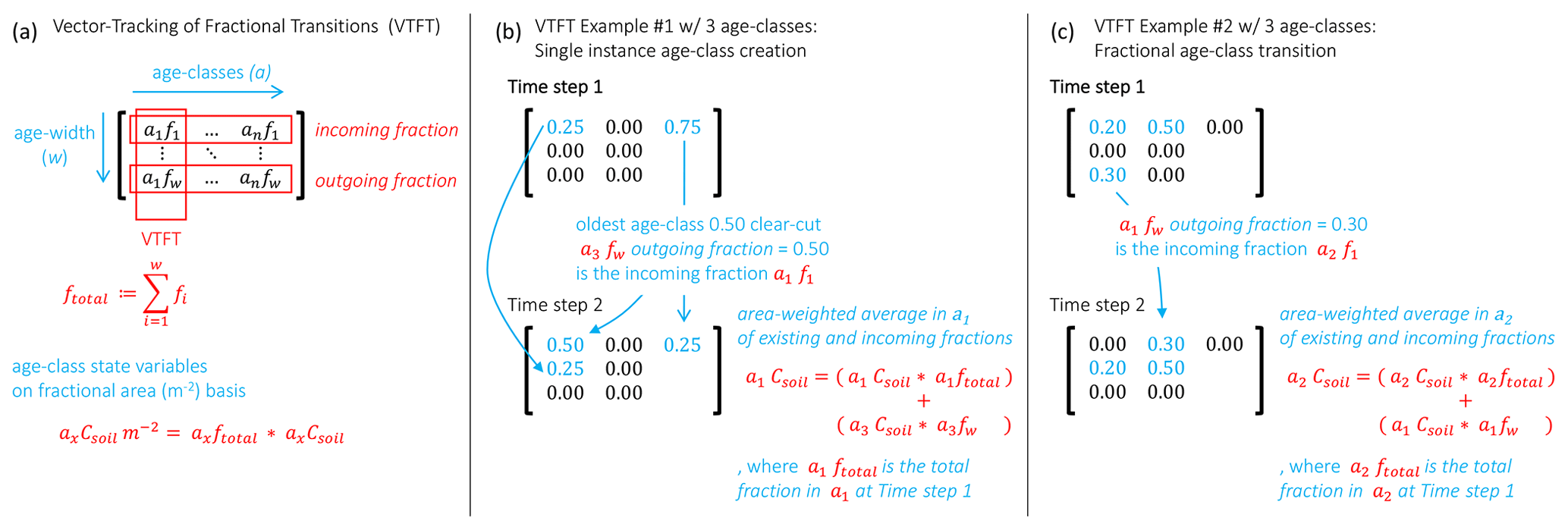
Figure 2Methodological examples of the matrix-based method called vector-tracking of fractional transitions for computationally efficient simulation of age classes in large-scale models. (a) Hypothetical matrix of VTFT vectors of fractional areas (f). The total area of the age class is the sum of the fractional areas in the corresponding VTFT vector. State variables are calculated on an area basis by accounting for the fractional area of the age class; in this example, Csoil is the carbon in soil. (b) An example of the VTFT method for a newly created age class by clear-cut wood harvest. An area-weighted average updates age-class state variables in the youngest age class using the preceding total fractional area of the age class and the incoming fraction. (c) A VTFT example for a fractional age-class transition. An area-weighted average updates state variables in an age class using the preceding total fractional area of the age class and the incoming fraction from the younger age class.
Two hypothetical scenarios are provided in Fig. 2 that demonstrate age-class transitions using the VTFT procedure when there is a young age class created, and when there are fractional age-class transitions between age classes. With VTFT, any number of age classes and age widths can be modeled, but it is demonstrated in this study that the age widths employed in this study are sufficient to minimize the dilution of state variables when area-weighted averaging is used to merge fractional age classes while also simulating stand–age patterns in state variables of carbon stocks, stem density and fluxes.
2.2.2 Integration with fire and LUCLM modules
The disturbance processes of simulated fire, land-use change, and land management can occur on multiple age classes at a time. That is, these processes are related but independent. For instance, fire can occur independently on each age class, and each age class would have its own independent estimate of the probability of fire. Wood harvest occurs first on the oldest age class and progressively harvests younger age classes until two demands are met (harvest area and harvest biomass), described in detail in the relevant section below. Clearly, each process influences the other as logging or fire both remove biomass that could be potential fuel for a future fire or biomass for a future harvest. These relationships are not evaluated here but are noted for their potential importance. Below, we describe in detail the integration of the age-class module with the two prominent forms of disturbance: fire and LUCLM.
Fire. The fractional area burned initiates the creation of a youngest age class, or it gets merged with a youngest age class if one exists already. Fire simulation is based on the semi-empirical Glob-FIRM model by Thonicke et al. (2001), with implementation details described in Sitch et al. (2003). In short, fire is dependent on the length of the fire season, calculated as the number of dry days in a year above a threshold and a minimum fuel load, defined only as the mass of carbon in litter. When a fire occurs, PFT-specific fire resistances determine the fraction of the PFT population that gets burned. The biomass of burned PFTs, along with the aboveground litter in the age class, gets calculated as an immediate flux to the atmosphere. The fraction of the PFT population that does not burn maintains state variables (e.g., tree height, carbon in leaf and wood) at previous values. It is possible to have so-called “survivor” trees on the youngest age class that then skew the age-height distribution of the age class. The model does not assume any structure of survivor trees. Instead, survivor trees occur as a function of the underlying process. For example, if a fire occurs on a stand, but the fire does not burn all the PFTs, then there will be survivor PFTs on the stand. Both fire and wood harvest (below) are simulated based on fractional area, and it is the fractional area, specifically, that gets reset to a young age class.
LUCLM. Age classes get created when managed land (i.e., crop and/or pasture) is abandoned and allowed to regrow into secondary forests, or when wood harvest occurs on forested lands and causes deforestation. In both cases, the fractional area abandoned or logged initiates the creation of a youngest age class, or it gets merged with a youngest age class if one exists already. To improve the account of primary forests, defined here as natural land without a history of LUCLM, and second-growth forests, defined as natural land with a history of LUCLM, transitions between these classes are unidirectional from primary to secondary. In the LUCLM module, gross transitions between land uses are simulated (Pongratz et al., 2014; Stocker et al., 2014), such that if the fraction of abandoned land equals the fraction of land deforested in the same year (net zero land-use change), then the fluxes from the gross transitions are tracked independently and give an overall more accurate account (and higher magnitude) of emissions from LUC than if we only tracked net transitions (Arneth et al., 2017).
General rules distinguishing primary and secondary stands within the age-class context stem from the Land Use Harmonization dataset version 2 (LUHv2; Hurtt et al., 2020) but with the following modifications so that the LUHv2 data can be used in LPJ-wsl v2.0. (1a) The primary grid cell fraction only decreases in size and never gets mixed with existing secondary forests or with abandoned managed land. Only fire creates young age classes on primary lands. (2a) Secondary grid cell fractions can be mixed with other secondary forest fractions, recently abandoned land, fractions with wood harvest, and recently burned area. General priority rules for deforestation and wood harvest. (1b) For simplicity, deforestation (i.e., land-use change) always occurs in the ranking of oldest to youngest age class, proceeding to deforest each age class until the prescribed fractional area of deforestation is met. This rule will always result in greater land-to-atmosphere fluxes than if rules were employed that allowed younger age classes to be preferentially deforested. (2b) Wood harvest (i.e., biomass harvest) also occurs in the ranking of oldest to youngest age class until two conditions are met. Timber harvest occurs on each age class until a prescribed harvest mass or harvest area is met.
Treatment of immediate emissions and residues. Deforestation results in 100 % of heartwood biomass and 50 % of sapwood biomass being stored for delay emission in product pools; root biomass is entirely part of belowground litter pools, while 100 % leaf and 50 % of sapwood biomass becomes part of aboveground litter pools. Grid cell fractions that underwent land-use change were not mixed with existing managed lands or secondary fractions until all land-use transitions had occurred. This avoids a computational sequence that results in a lower flux if deforestation and abandonment occur in the same year. For wood harvest, 100 % of leaf biomass and 40 % of the sapwood and heartwood enters the aboveground litter pools, and 100 % of root biomass the belowground litter pools; 60 % of sapwood and heartwood are assumed to go into a product pool for delayed emission.
Timber from deforestation and harvest in product pools for delayed emission (Earles et al., 2012). For deforestation, 60 % of exported wood (i.e., not in litter) goes into a 2-year product pool, and 40 % goes into a 25-year product pool, following the 40:60 efficiency assumption from McGuire et al. (2001). For wood harvest, the model uses space–time explicit data on harvest fractions going into roundwood, fuelwood, and biofuel product pools. We use three product pools and assume that 100 % of the fuelwood and biofuel fraction goes into the 1-year product pool (emitted in the same year of wood harvest), 50 % of the roundwood fraction goes into the 10-year product pool (emitted at rate 10 % per year), and the remaining 50 % of the roundwood fraction goes into the 100-year product pool (emitted at rate 1 % per year).
2.3 Experimental design and analysis
2.3.1 Model inputs
Inputs to the model are gridded soil texture (sand, silt, clay fractions) from the USDA Harmonized World Soils Dataset v1.2 (Nachtergaele et al., 2008), annually varying global mean [CO2] (time series available in the Supplement), and monthly varying air temperature, precipitation, precipitation frequency, and radiation from the Climate Research Unit (CRU, version TS3.26) data for 1901–2016. Land use, land-use change, and wood harvest were prescribed annually based on LUHv2 (Hurtt et al., 2020), which is used as forcing land use for the sixth Coupled Model Intercomparison Project (CMIP6; Eyring et al., 2016). The dataset includes fractional area of bi-directional (gross) land-use transitions between forested and managed lands, as well as the total biomass of wood harvest on a specified fractional area logged. In LPJ-wsl v2.0, managed lands (i.e., crop and/or pasture) are treated as grasslands with no irrigation, no fire, and tree PFTs were not allowed to establish. Model representation of land management is an oversimplification to focus on effects of wood harvest.
2.3.2 Examining age dynamics: qualitative evaluation of regional simulations against the US Forest Inventory Analysis data to assess simulated changes in stand structure and ecosystem function
US Forest Inventory and Analysis (FIA). The FIA dataset is freely available at the FIA DataMart web portal (FIADB version 1.6.0.0.2), accessed 2 February 2016. The FIA plot-level data are composed of four circular subplot sample areas (168 m2), wherein attributes of all trees with diameter at breast height (DBH) ≥5.0 in (12.7 cm) diameter are recorded. We extracted variables that capture two main axes of structural change as a function of forest age: stem density and tree height. Spatial coordinates of sample plots are “fuzzed” with imposed error for privacy reasons (FIA User Guide v 6.02; O'Connell et al., 2015). For purposes of this analysis, plot data were aggregated to the spatial scale of the US Forest Service Divisions (Fig. S2; USFS Divisions are delineated by regional-scale precipitation levels and patterns as well as temperature) minimizing co-location concerns between model–observation comparisons. We filtered the FIA data based on the following criteria. We only included plots that used the national standard plot design (DESIGNCD of 1) and were located on forested land (COND_STATUS of 1) with no history of major disturbance, stocking, or logging (DSTRBCD of 0; TRTCD1 of 0), which could alter natural patterns of tree density versus age and confound the comparison to simulated data. We also only included plots that had both subplot samples of live tree (STATUSCD of 1) stem density and also circular micro-plot (13.5 m2) stem density samples of seedlings and/or saplings (defined as trees 1 to 5 in (2.54 to 12.7 cm) in diameter), and where the subplot sampling design was the national standard (tree table SUBP of [1,4]); LPJ-wsl v2.0 implicitly includes sapling and adult trees in estimates of tree height and stem density. We assumed that the filtered plots were representative of the true density and distribution of tree species for the general vicinity of the plots and of the USFS Division. Although these requirements for selecting FIA plots reduce the total amount of data, we aimed to make evaluations in a fair manner, in both spatial scale and meaning.
Table 2Description of LPJ-wsl v2.0 simulations in this study, corresponding objectives and related science questions.
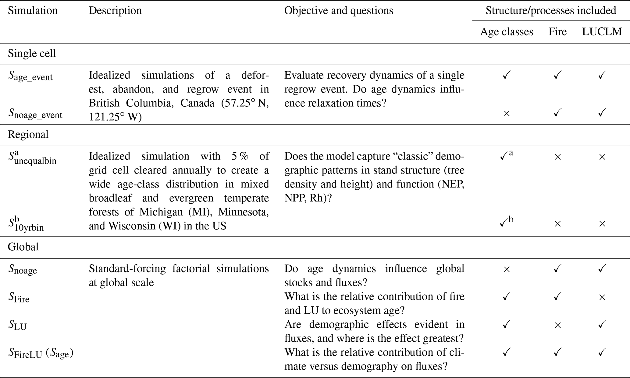
a Unequal age-width simulation. Age widths are as described in Table 1. b The 10-year interval age-width simulation. Age widths are as described in Table 1.
Regional simulations. The objectives of the regional simulations (Table 2) were to evaluate demographic patterns of stand structure and function when simulating age classes using different age-width binning. Two idealized simulations were conducted at a regional scale to sample simulated annual stem density, average tree height, and NEP. The first simulation used the unequalbin age-width setup, Sunequalbin, and another used the 10-yr-equalbin age-width setup, S10 yr bin (Table 2). For both simulations, fire and LUCLM were not simulated. Instead, 5 % of the fractional area of age classes >25 years were cleared of biomass annually; the fractional area cleared was reclassified and merged with the youngest age class. The intent of the setup was to ensure that each grid cell maintained fractional area in every age class for each year of the simulation and avoided situations in which age classes were only present in “bad years”, or when growing conditions were poor. Both simulations were conducted with a 1000-year “spinup” using fixed CO2 (287 ppm, “pre-industrial” values) and climate randomly sampled from 1901–1920 to ensure that age distributions were developed and state variables were in dynamic equilibrium (i.e., no trend). A transient simulation then used time-varying CO2 and climate, as prescribed by model inputs. Stand structure data were analyzed for 1980–2016.
The idealized simulations were performed for the mixed deciduous and evergreen forests of Michigan, Minnesota, and Wisconsin in the US (bounding box defined by left: 97.00∘ W; right: 82.50∘ W, top: 49.50∘ N, bottom: 42.00∘ W). These forests are of moderate temperate climates, with total annual rainfall 815.0 mm yr−1 (average over 1980–2016, based on CRU TS3.26), a time-series minimum of 21.0 mm per month, and a maximum of 148.5 mm per month. Mean annual temperature (1980–2016, CRU TS3.26) was 5.98 ∘C with monthly minimum of −11.45 ∘C and maximum 20.98 ∘C.
Data were pooled for the region over the time period and by age class. Data were plotted in boxplots to show median value, interquartile range, and outliers. No attempt was made to detrend data because there was enough between-age-class variation to evaluate general demographic patterns visually.
2.3.3 Examining resilience: idealized simulation of a single event of deforestation, abandonment, and regrowth
The objective of the idealized simulation was to evaluate the effect of age classes on relaxation times following a single deforestation, abandonment and regrowth event within a single grid cell (Table 2). The relaxation time is defined as the time required for a variable to recover to previous state and is a direct measure of ecosystem resilience (sensu Pimm, 1984). Two simulations were conducted, the first simulation used the 10-yr-equalbin age-width setup, Sage_event, and another did not simulate age classes, Snoage_event (Table 2). Both simulations were conducted with a 1000-year “spinup” using fixed CO2 (287 ppm, pre-industrial value) and climate randomly sampled from 1901–1920 to ensure that state variables were in dynamic equilibrium. A transient simulation then used time-varying CO2 and climate, as prescribed by model inputs. Fire and LUCLM were not simulated. Instead, 25 % of the fractional area was deforested in year 1910 of the simulation and classified as managed land. Treatment of deforestation byproducts (i.e., carbon in dead wood left on site) were the same in both simulations. In the following year (1911), the managed land fraction was abandoned and allowed to regrow. The following state variables were plotted over time and visually evaluated: net biome production (NBP, defined as the difference between NEP and LUC_flux), NEP, net primary production (NPP), heterotrophic respiration (Rh), and carbon in biomass.
The idealized simulations were performed for a single grid cell in a mixed broadleaf and evergreen needleleaf forest in British Columbia, Canada (57.25∘ N, 121.25∘ W). The grid cell is a boreal climate with total annual rainfall 473.7 mm yr−1 (average over 1980–2016, based on CRU TS3.26) with monthly minimum 9.11 mm per month and maximum of 105.8 mm per month. Mean annual temperature (1980–2016, CRU TS3.26) was 0.59 ∘C with a monthly minimum of −16.9 ∘C and maximum 14.7 ∘C.
2.3.4 Global simulation objectives and setup
There were three main objectives for global simulations. The first objective was to evaluate the contribution of age-class information to global stocks and fluxes. Here, a simulation with age classes (Sage) was compared to a simulation without age-class representation (Snoage) (Table 2). The second objective was to determine the relative influence of fire and LUCLM on the spatial and temporal distribution of ecosystem ages. For this objective, a fire-only simulation (SFire) had age classes only created by fire, whereas a LUCLM-only simulation (SLU) had age classes only created by abandonment of managed land or by wood harvest (Table 2). A simulation with both fire and LUCLM (SFireLU) was used as the baseline for comparison against SFire and SLU. The third and fourth objectives used data from Sage (Sage=SFireLU) to determine where the effect of demography was greatest and to identify the relative influence of demography versus climate on simulated fluxes (NEP, NPP, and Rh).
For all global simulations, a spinup simulation was run for 1000 years using randomly sampled climate conditions from 1901–1920 and atmospheric CO2 fixed at pre-industrial levels (287 ppm) and no land use or wood harvest; spinup ensured that age distributions and state variables were in dynamic equilibrium (i.e., no trend). For simulations with land use, a second “land-use-spinup” procedure was run for 398 years to initialize land-use fractions of crop and/or pasture to year 1860, resampling climate and fixing CO2 as in the first spinup. After spinup procedures, climate and CO2 were allowed to vary until simulation year 2016; in SLU and SFireLU, land-use change and wood harvest varied annually as prescribed by the LUHv2 dataset.
In the first objective (as above), global values for stocks and fluxes include both natural and managed lands. These global estimates conform to typical presentation of global values (Le Quéré et al., 2018), in petagrams (1015) of carbon. Comparisons are made among simulation types and to values from the literature.
For the second objective, a time series of zonal mean ecosystem ages were analyzed to determine the relative importance of SFire and SLU on the observed distributions in SFireLU. The first assessment was made by visual inspection of zonally averaged time series (i.e., Hovmöller plots) for the entire period of transient simulation (1860–2016). In addition, for each of SFire and SFireLU, a simple linear regression model (age is equivalent to β0+β1 ⋅ year, setting 1860 as the reference year and defined as 1) was applied to identify trends in ecosystem age by the following zonal bands: boreal (50 to 90∘ N), temperate (23 to 50∘ N), and tropics (23∘ S to 23∘ N). Trends in age distributions due to LUCLM are not prescribed by inputs per se; instead, the age module is a necessary model structure that allows full realization of the effect of forcing data on age distributions. Trends in age distribution due to fire, which is a simulated process as opposed to prescribed, result from climate and fuel load feedbacks on fire simulation.
2.3.5 Statistical model to assess relative importance of demography and climate
For the third objective of global simulations – to reduce dimensionality of the data and to assess the relative influence of demography and climate on simulated fluxes – annual flux data from Sage (Table 2) were analyzed from 2000–2016 using a generalized linear regression model:
where “flux” was either NEP, NPP, or Rh in kg C m−2 yr−1, precipitation (mm) and temperature (Celsius) data from CRU TS3.26, and “ageclass” was categorical, defined by the age-class code (Table 1), and the beta coefficients (B) for subscripts of grid cells (i), years (yr), and age class. The beta coefficients are therefore unique to every grid cell, and the betas for age classes are estimated separately for each age class within the grid cell (B3i,age). An initial test of the model attempted to estimate globally consistent predictor effects, but the model was found to be a poor fit (not shown) and it was assumed that there was too much variation among grid cells to detect globally consistent effects. Instead of adding additional gridded fields of predictor variables to account for grid-cell-level variation, the same statistical model was applied and analyzed per grid cell. This allowed coefficients of precipitation, temperature and “ageclass” to vary by grid cell, in essence, reducing the effect of variation in PFT composition, soil texture, and hydrology that might otherwise reduce predictive power.
In all grid cell analyses, the intercept term was intentionally omitted from the data model by adding a “−1” term to the data model. The “ageclass” term in the statistical model (B3i,age), as a categorical variable, effectively takes the place of the intercept term anyhow, so the outcome is that estimates are for the absolute effect of each age class on the predicted flux as opposed to estimates that were relative to the first age class; this had no impact on estimated coefficients but it did simplify analyses. In grid cells where only a single age class was present, the statistical model was defined as (flux total_precipitation mean_temperature), leaving the intercept term, in this case – B3i, to be estimated from the data and then reclassifying the intercept term by the age-class code for the grid cell.
The degrees of freedom (DoFs) of a model for a grid cell with a single age class was 14 DoFs, based on 17 annual data points to estimate coefficients of three predictors. The degrees of freedom for a grid cell that had a maximum of 12 age classes was 190 DoFs, based on 204 annual data points to estimate coefficients for 14 predictors. Because the analysis produced statistical results for every grid cell, the degrees of freedom are not presented elsewhere. Coefficients were only analyzed or mapped when significant at p=0.05.
3.1 Model stand structure – comparison against inventory data
FIA data were not equally available for every age class, nor for every division (Fig. S2), but there were enough inventory data across eight divisions, spanning subtropical to temperate steppe climates, to qualitatively suggest that LPJ-wsl v2.0 does capture the expected patterns of tree density and height per age in the different climates evaluated. There was a tendency for LPJ-wsl v2.0 to overestimate stem density in younger age classes and systematically underestimate tree heights among age classes (e.g., Figs. S3, S5), for which the greater number of small individuals could cause the average tree heights to be dampened. However, LPJ-wsl v2.0 is a big-leaf, single-canopy model that include space-filling “packing” constraints on stem density, based on allometric rules for size and height of PFTs. Also the model does not represent multiple PFT cohorts in an age class, or more simply, it does not represent vertical heterogeneity such as understory growth that would otherwise increase stem density. As such, and under the current model architecture and associated assumptions, the exact cause of the mismatch is unclear. Even still, the more general pattern of modeled stem density and tree height tended to track FIA data, with stem density being maximal in the younger age classes and declining thereafter, whereas tree height patterns increased more linearly before stabilizing (Figs. S6 to S9).
FIA data had greater variability among age classes, regardless of division. FIA data are not aggregated by PFT, instead they are species-level data. Changes in species composition over time do occur and can add to the observed variability among age classes in tree density and tree height. LPJ-wsl v2.0 includes a limited set of PFTs, which most likely limits the model's capacity to represent similar levels of variation in tree density and tree height. It is beyond the scope of this study to disentangle these patterns further, but greater agreement between observed and simulated patterns of forest structure might be achieved by including additional plant functional types that are representative of tree species for a given division.
3.2 Model age dynamics
3.2.1 Dynamics of stand structure and function – regional simulations
Forest structural characteristics of stem density, height, and NEP followed the expected patterns with age with a few exceptions. In Sunequalbin (Table 2), stem density increased from near zero to maximum in the 21- to 25-year age class, before declining non-linearly (Fig. 3). By contrast, the gradual increase in stem density in the first age class in S10−yrbin (Table 1) was not readily apparent because this process, which is evident in Sunequalbin, occurs entirely within the youngest 1- to 10-year age class in S10−yrbin. Both simulation setups approach the same stem densities after age ∼25; prior differences are due to binning of age widths.
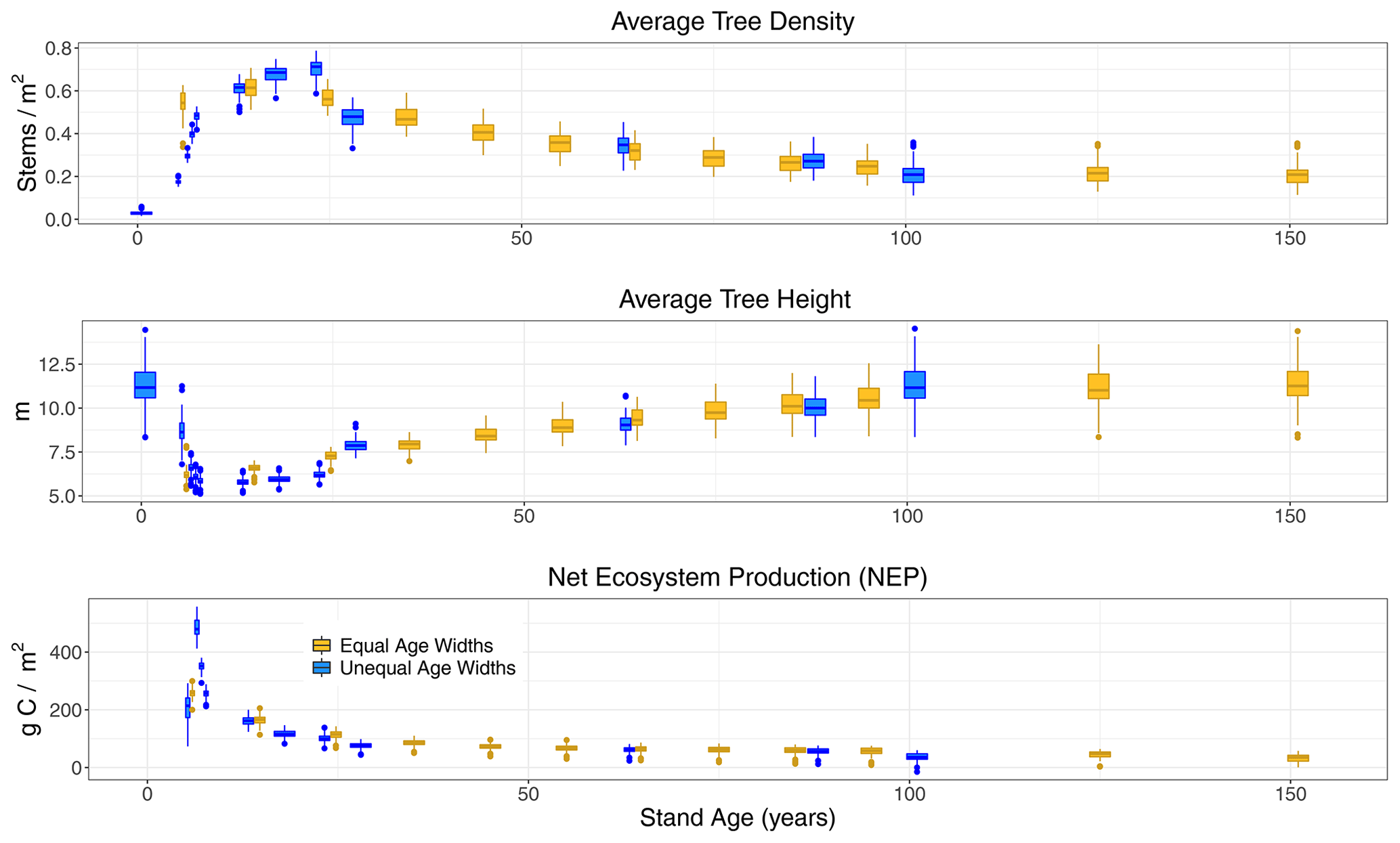
Figure 3Boxplots by age classes (x axis, in years) from LPJ-wsl v2.0 simulations for US states of MI, MN, and WI. Data are from (yellow) simulations using equal age widths and (blue) simulations using and unequal age widths (see Table 1). Data are plotted on the x axis at the middle age of the age-class bin; note that the last age-class bin for either simulation is defined as +151 years (equal bin) and +101 years (unequal bin). For average tree height (middle row), large tree heights in the youngest age class of the unequal-bin simulation (blue) represent so-called “survivor” trees.
For average tree height in Sunequalbin, there were large tree heights in the youngest age class, which results from so-called “survivor” trees (Fig. 3). Not all trees are killed off when a disturbance occurs in LPJ. Although the age class is “reset” to the youngest age class, the survivor trees skew the height distribution until the density of establishing saplings subsequently increases and brings down the average tree height to smaller values. This pattern is more akin to what occurs during natural fires or selective harvesting, which can reduce the overall age but might not result in a complete removal of all trees. By contrast, the skewed age-height pattern is not apparent in S10−yrbin (Fig. 3) only because the same process is effectively hidden. Both simulation types approach the same average tree heights after age ∼25 (Fig. 3).
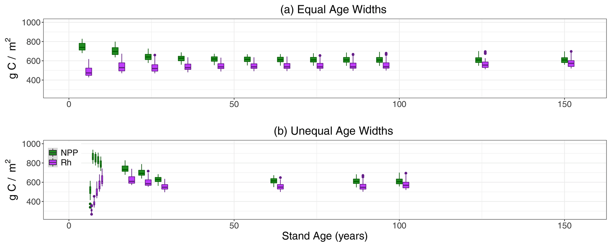
Figure 4Boxplots of NPP and Rh by age classes (x axis, in years) from LPJ-wsl v2.0 simulations for US states MI, MN, and WI, for simulations using (a) equal-bin age widths and (b) unequal-bin age widths.
NEP peaked at age classes 5–6 in Sunequalbin, before declining non-linearly to the lowest average value in the oldest age class (Fig. 3). Although the unimodal peak was not apparent in S10−yrbin, the maximum NEP occurred in the youngest age class and also declined non-linearly thereafter (Fig. 3). The decline in NEP after a maximum at 5–6 years was driven mainly by an increase in Rh due to increases in turnover rather than a larger decline in NPP (Fig. 4). The peak in NEP did not coincide with maximum tree density at ∼20 years. Instead, model dynamics suggest that the total foliar projective cover of tree canopies reaches near maximum (80 %–95 % cover; not shown) at 5–6 years, thereafter plant competition reduces NPP while biomass turnover increases, which together cause the apparent decline in NEP. The time period of canopy closure, at 5–6 years, in LPJ-wsl v2.0 is probably too early, in part due to advanced regeneration (saplings establish at 1.5 m height) and constant establishment rates. The age-class module qualitatively demonstrates NEP–age relationships consistent with field-based evidence (Ryan et al., 2004; Turner, 2010).
Lastly, an emergent pattern was found in the declining portion of the NEP–age curve and approximately follows the functional form NEPmax ⋅ 0.70age−agemax, where “NEPmax” is the maximum NEP flux at the initial point of decline, “age” is the age of the patch, and “agemax” is the age of the patch where NEP is maximized. Thus, the non-linear decline in NEP is approximately 30 % with increasing age. The functional equation holds between years 5–6 and year 25, after which NEP decreases only by 20 % with increasing age and the functional form becomes NEP, where NEP25yr is the NEP at year 25. The functional form of the decline in NEP is consistent among climate regions when simulated data are analyzed separately for all US states (not shown). The binning strategy is likely not a determinant of this pattern between NEP and stand age, which is evident in Fig. 3 for both age-class setups. In this regard, we care less about the binning strategy and more that the emergent pattern is reflective of simulated model dynamics. This emergent pattern could lend itself to observational constraints if similar emergent patterns can be derived from forest inventory data in the future.
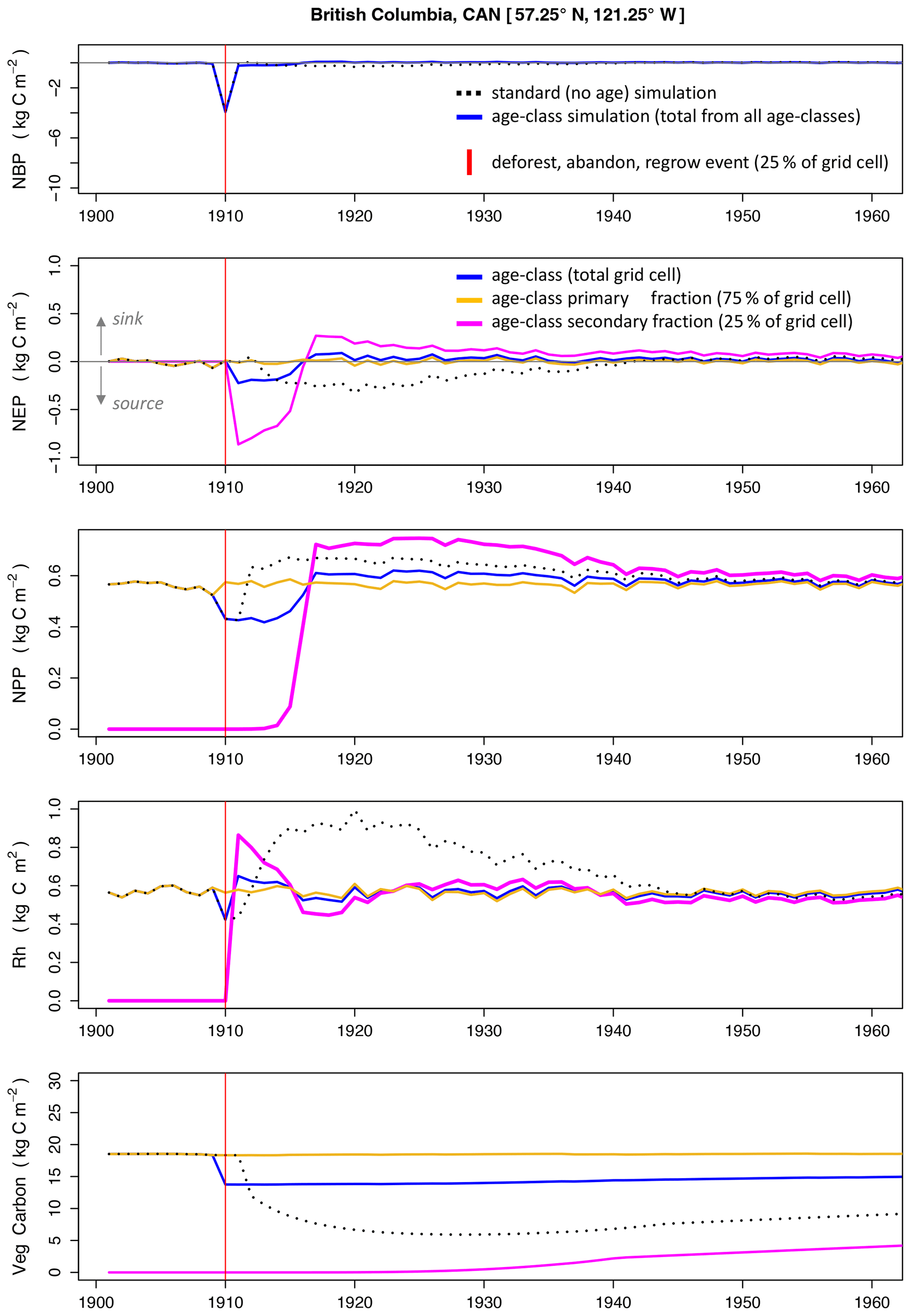
Figure 5A time-series comparison between the standard LPJ-wsl v2.0 simulation (Snoage_event) and the age-class approach (Sage_event) in an idealized single-cell simulation of a deforestation, abandonment, and subsequent regrow event. The x axis is the simulation year. See Table 2 for simulation details.
3.2.2 Time-series evolution of a deforestation, abandonment, and regrow event
A single event of deforestation, abandonment, and subsequent forest regrowth caused long-lasting effects on carbon balance and dynamics when omitting age-class dynamics. In the simulation without age classes, Snoage_event (Table 2), grid-cell-level NEP takes ∼30 years to recover to values prior the event, whereas the age-class simulation, Sage_event, takes only 5–6 years to recover (Fig. 5) – a 5-fold change in relaxation times. The quick recovery of grid-cell-level NEP in Sage_event is due partly to the fact that the fraction of the grid cell (75 %) that was not deforested maintained its state variables (carbon stocks in vegetation, soil, litter) unchanged from its prior state, which buffered NEP and dampened the effect of the smaller fraction (25 % of grid cell) that was deforested. Age-class dynamics also contributed an elevated NEP (Fig. 5) that quickens the recovery at the grid cell level. In Sage_event, there is an elevated NEP in the secondary stand that is sustained for more than 30 years following the event.
In Snoage_event, vegetation dynamics cause turnover to increase and cause an elevated grid-cell-level Rh that is consistently higher than grid-cell-level NPP for 30 years after the event. This pattern is striking because NPP recovers quicker than in Sage_event and maintains an elevated value for ∼30 years. Following a disturbance event in LPJ, stem density and foliar projective cover is reduced but the state variables (carbon in plant organ pools of leaf, stem, root) maintain prior values; this is the reason grid-cell-level NPP recovers quickly in the standard no-age simulation. As stand density increases again, canopy closure initiates competitive dynamics that result in mortality of individuals of the plant population that are generally larger than if the stand had progressed from small to large individuals (as in Sage_event).
The VTFT module also uses the mean-individual approximation but stand dynamics are always allowed to occur in natural progression and the relatively small age widths (10 years) ensure that stand age dynamics (NEP–age trajectories in Figs. 3 and 4) most evident in the first 50 years are discretely modeled. To reiterate, we think that the simulated flux dynamics in the no-age simulation is a pure model artifact. What we mean by that is that a patch-based (age-class) model is more like reality, where the full “grid” of space is an explicit representation of unique patches of ecosystem. Whether or not the recovery times themselves are accurate (30 years versus 5 years) is less concerning at this point. The growth rates and recovery trajectories will likely have to be optimized, ideally, to observed patterns, but this is beyond the scope of this paper.
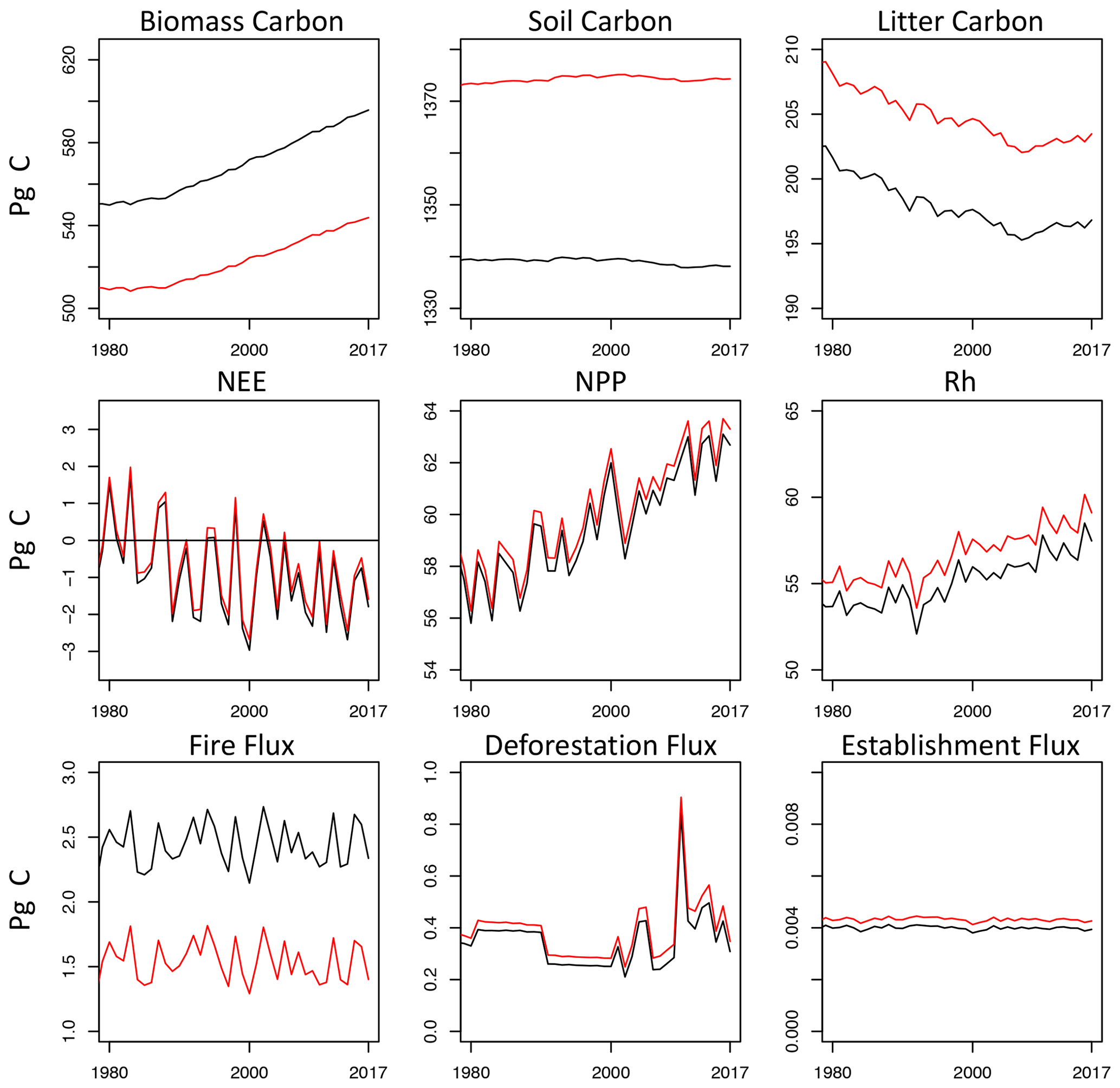
Figure 6Time series of global carbon stocks and fluxes from LPJ-wsl v2.0 simulation without age classes (black lines) compared against simulations with age classes (red).
3.3 Global stocks, fluxes, and age distribution
3.3.1 Stocks and fluxes – Snoage versus SFireLU and convergence in global NEP
Carbon stocks in biomass are lower in Sage than in Snoage by ∼40 Pg C globally (Fig. 6). Lower global biomass in Sage can be explained by feedbacks from LUC and fire that create younger age classes that have lower overall biomass than in older stands. In addition, age dynamics cause turnover to increase (as in Figs. 3 and 4), causing soil carbon to be greater by ∼35 Pg C and litter carbon to be greater by 5 Pg C. Taken together, age-class dynamics cause 40 Pg C to be re-allocated from the living biomass pool to the soil-detrital pool, which compounds to alter the magnitude of fluxes from heterotrophic respiration. Demographic changes in turnover, such as these, are already known to be a large source of uncertainty among projections by global ecosystem models (Friend et al., 2014). What these numbers emphasize, however, is that uncertainty among models could be reduced by explicitly modeling age dynamics.
Net ecosystem exchange (NEE; positive fluxes to atmosphere) is only marginally different between Snoage and Sage simulations (mean difference of 0.25 Pg C yr−1 over 2000–2010). Compensatory fluxes in fire and Rh explain the small difference in NEE at global scales. Fire fluxes in Sage are lower by 0.92 Pg C yr−1 in the 2000s than in the Snoage, but fluxes from Rh are greater in Sage by 1.61 Pg C yr−1 and NPP also greater by 0.55 Pg C yr−1. The fluxes in fire, Rh, and NPP largely offset to minimize differences in NEE from age dynamics.
The question still remains – should there be an expectation for greater differences in NEE? Consider that deforestation (areal changes prescribed the same in Snoage and Sage) occurs from the oldest to youngest age class in Sage, following greater to lower overall biomass, respectively. The deforestation flux is greater in the Sage by only 0.04 Pg C yr−1 in the 2000s compared to deforestation fluxes in Snoage, which makes sense given that low-biomass age classes are not preferentially deforested or harvested. By contrast, fire is not prescribed in LPJ-wsl v2.0 but it is simulated based on soil moisture and a minimum fuel load. It is not clear outright how age dynamics affect soil moisture, but fluxes from fire would need to be proportional to the biomass in an age class. By definition in Sage, there is explicit representation of lower-biomass age classes (i.e., younger) than in Snoage, and a series of fires or disturbances within the grid cell would drive the age distribution towards younger states, exacerbating differences in downstream fluxes as well. That global NEE only changed marginally when simulating global age dynamics was a surprise but explained by shifts in the carbon pools and compensatory fluxes, then the patterns appear to make sense. In light of these compensation effects, however, there is a great need to benchmark fluxes from critical feedbacks, particularly from fire in this case. It is beyond the scope of this paper to do so, and the best available datasets, such as the Global Fire Emission Database (GFEDv4s; van der Werf et al., 2017), do not lend themselves to direct comparison with fire fluxes from LPJ. GFED includes fires from deforestation and land management that are tracked differently in LPJ-wsl v2.0 – as a land-use change flux, which cannot simply be added to the fire flux for direct comparison to GFED without double counting. In any manner, this issue is stated as a suggestion for future development and refinement.
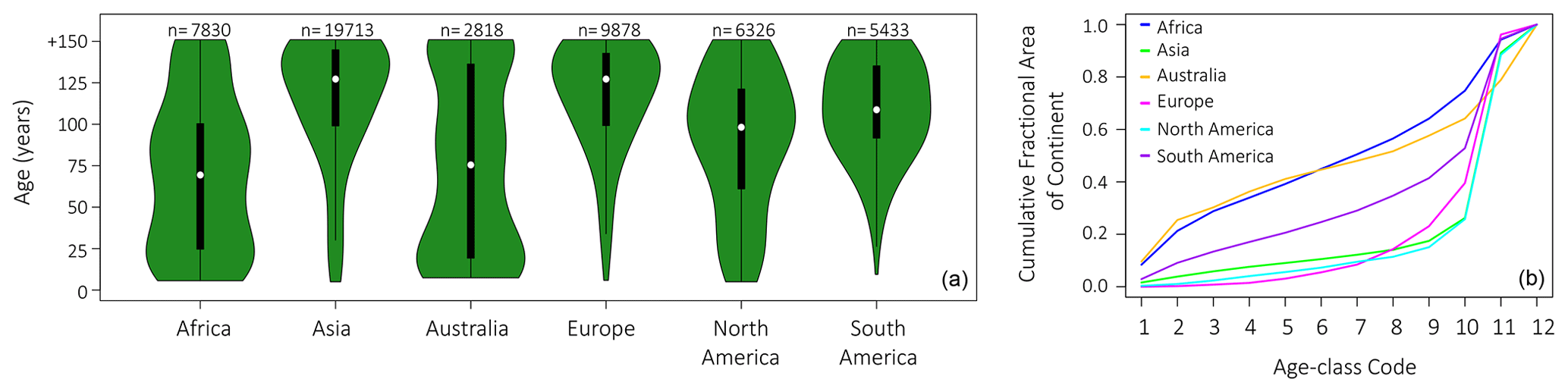
Figure 7Age-class distributions by continent. (a) Violin plots of ecosystem age by continent averaged over 2000–2010, based on LPJ-wsl v2.0 simulations. Violin plots show the distribution of data points (green), interquartile range (black box), and the median value (white circle). The number of vegetated 0.5∘ grid cells in each continent are above the plot. (b) Cumulative fractional area in continent by age classes. Age-class codes, lowest (youngest) to greatest (oldest), correspond to the 10-yr-equalbin age-class setup (Table 1).
3.3.2 Global age-class distribution – contribution of fire and LUCLM to age distributions
Average ecosystem age, generated by the model, differed greatly among continents (Fig. 7), with large areas of old-growth forests in Asia, Europe, North America, and South America skewing the distribution towards older ages. The largest area of young ecosystems was located in Africa and Australia (Fig. 1), wherein age classes comprised an age to fractional area ratio of vegetated land (age classes <20 years comprise ∼20 % of the vegetated land area in Africa and Australia and age classes <40 years ∼40 % of vegetated land area; Fig. 7).
Table 3Linear trend statistics by zonal band from LPJ-wsl v2.0 simulations, based on model (age year), where the year at 1860 is indexed at 1. Coefficients listed as μ± S.E. All DoFs are 113 and p<0.001.
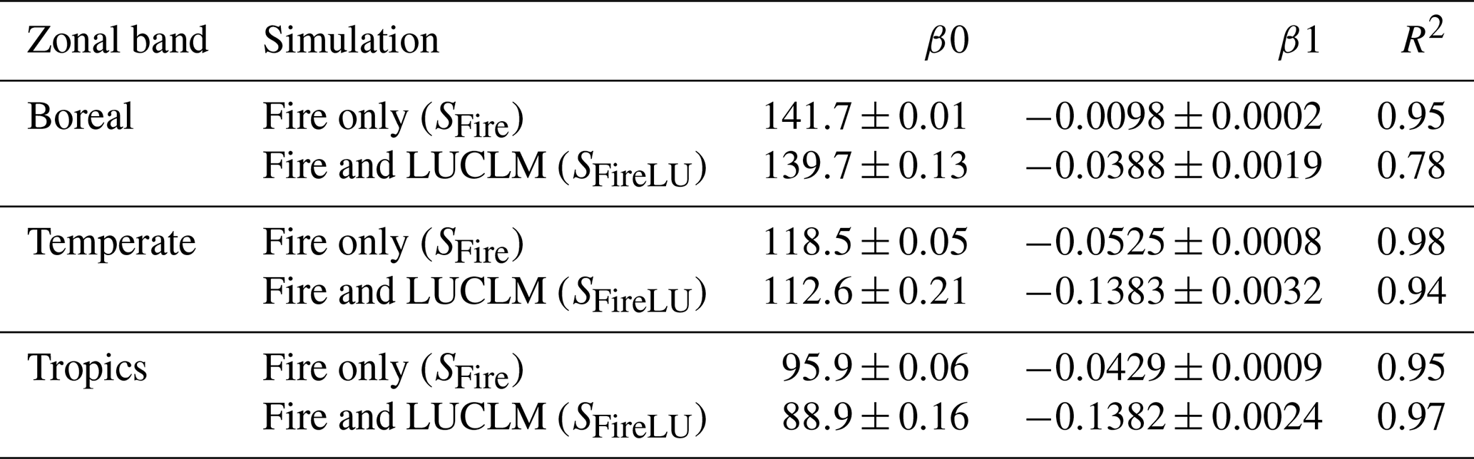
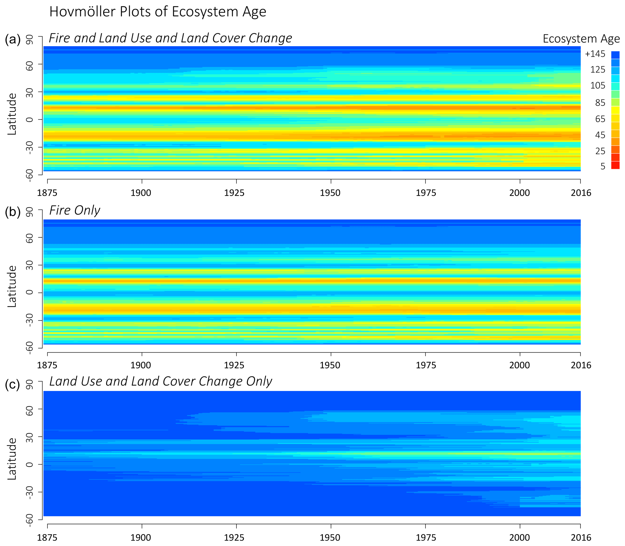
Figure 8Zonal ecosystem age versus year based on LPJ-wsl v2.0 simulations using full forcing (a), only fire (b), or only land-use and land-cover change (c).
Ecosystem age by zonal band was oldest at boreal latitudes, followed by temperature latitudes, and youngest in tropical latitudes, which was primarily the results of frequent fires in simulated grassland ecosystems. The primary driver of zonal age distributions was fire (Fig. 8). According to results from the statistical model (Table 3), the average age difference due to fire among zonal bands in 1860 was 23 years between boreal (older) and temperature (younger) latitudes, and it was 32 years between temperature (older) and tropical (younger) latitudes. The difference in ecosystem age among zonal bands increased to 60 years in simulation year 2016 between boreal and temperate latitudes, while the difference in ages between temperature and tropical latitudes remained similar (31-year age difference). There was a statistically significant decrease in zonal ecosystem age over time due to fire (Table 3), most likely from feedbacks due to enhanced fuel (biomass) production from CO2 fertilization. The causes were not explored further because feedbacks between fire–climate–CO2 are largely constrained by the fire module itself. The emphasis here is simply that fire was a major driver of age distributions and fire–age relationships had an apparent trend over time. Between simulation years 1860 and 2016, fire caused a total change in ecosystem age, integrated over the time period, by −1.5 years in boreal zones (negative values for a decrease in age), whereas the change was greater in temperate (−6.7 years) and tropical (−8.24 years) zonal bands (Table 3). The larger trend in temperate and tropical latitudes might be due to increasing warming temperatures in contemporary times, causing drier conditions more suitable for fire, or from increases in fuel loads from CO2 fertilization. A more convincing argument would require support from additional factorial experiments to identify to the casual driver of the trend differences.
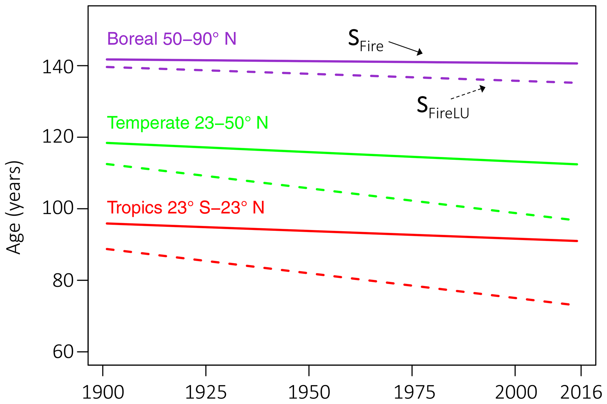
Figure 9Trend in ecosystem age by zonal band for LPJ-wsl v2.0 simulation with only fire (SFire, solid lines) and with both fire and LUCLM (SFireLU, dashed lines). Fire causes zonal bands to differ in ecosystem age by ∼23 years and decreases the average age by 0.009 to 0.054 yr−1. LUCLM decreased ecosystem age at rates up to 3 times the rate of fire, from 0.038 yr−1 in boreal zones to 0.138 yr−1 in temperate and tropical zones.
After accounting for the effects of fire, LUCLM caused a much greater change over time in the zonal ecosystem age (Fig. 9). Integrating from 1860 to 2016, LUCLM caused a zonal change in ecosystem age by −6.1 years in boreal zones, whereas the change in ecosystem age from LUCLM in temperate and tropical zones was −21.6 years, with no significant difference in the trend due to LUCLM among these zonal bands (Table 3). These patterns are consistent with the concentration of deforestation in the tropics and land-use change in temperate latitudes, as described by the forcing data (Hurtt et al., 2011, 2020).
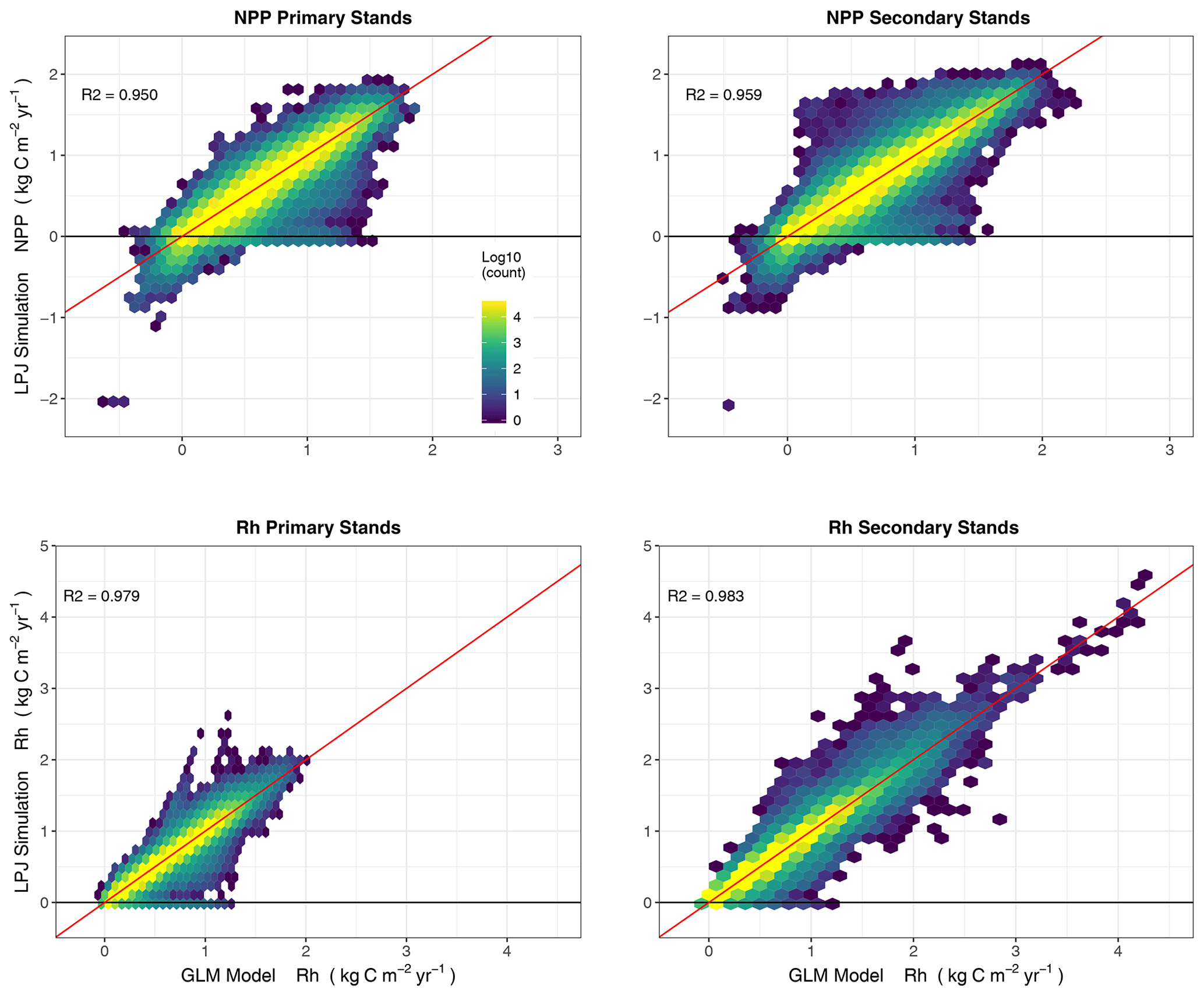
Figure 10Annual fluxes (NPP, Rh) (2000–2017) from LPJ-wsl v2.0 simulations versus predictions of LPJ-wsl v2.0 fluxes based on a generalized linear model (GLM; flux is the sum of precipitation, temperature and age class); coefficients were allowed to vary by grid cell, in essence, reducing the effect of variation in plant composition, soil texture, and hydrology. Coloring is by density of grid cells on a log scale; diagonal red line is the 1:1 correspondence line. The simplified statistical model can simplify the dynamics in the global vegetation model, with coefficients from the GLM helping to determine the relative importance of a small set of predictors.
3.4 Global demographic effects on NPP and Rh
3.4.1 Simplification of LPJ-wsl v2.0 via a statistical model
The statistical model (flux being the sum of B1 precipitation, B2 temperature and B3age age class; see Sect. 2.3.5 for details) was able to estimate simulated NPP and Rh with great predictive power, with R2 values between 0.95–0.98 (Fig. 10). The predicted fluxes were at annual timescales, with annual variation being mainly driven by total annual precipitation and mean annual temperature, whereas the mean state (intercept) being predicted by the age class. The predictive power for a model of NEP was worse (R2 between 0.60–0.65; Fig. S1). The effect of precipitation, temperature, and age class on NEP was not consistent enough for robust predictions, but more specifically, the predictors had different effects on NPP versus Rh leading to poorer model fit. As it is, NEP is better derived as predictions of NPP minus predictions of Rh rather than having a stand-alone model for NEP.
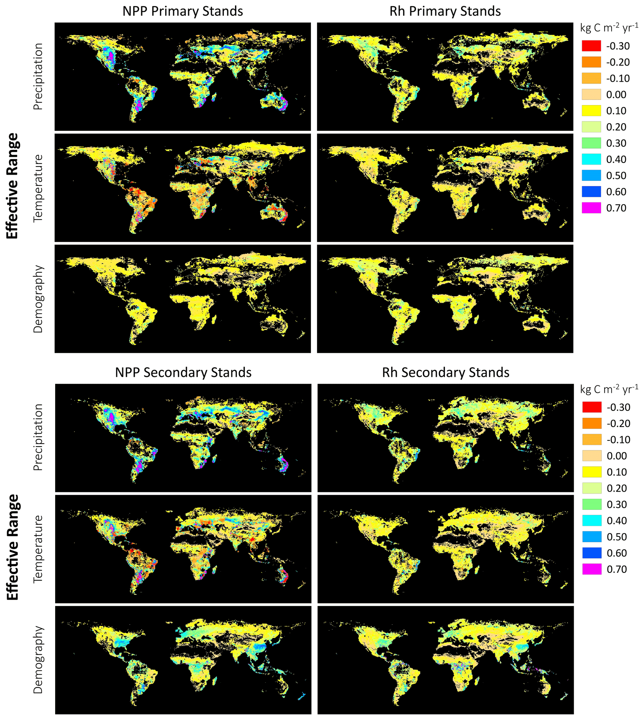
Figure 11Global maps of the Effective Range of the Predictors (precipitation, temperature, demography) on LPJ-wsl v2.0 fluxes (NPP, Rh); black indicates zero values or no data. The effective range of the predictor is calculated as the grid-cell-specific beta (β) coefficient multiplied by the observed range of the predictor variable for the grid cell, for the years 2000–2017. Units are on the scale of the predicted flux (kg C m−2 yr−1). In these maps, an emphasis is placed on the effective range of the predictor rather than the absolute value of the coefficient, although these too can be mapped for forecasting purposes. See Sects. 2.3.5 and 3.4 for additional details.
3.4.2 The effective range of predictors – assessing relative importance of demography on predicted fluxes
The “effective range of the predictors” was mapped to visualize spatial patterns of the range of effects, given observed values for the predictors (Fig. 11). In essence, the effective range of the predictor is a measure of the dynamic range in the predicted flux due to changes in precipitation, temperature or demography. It is calculated as the grid-cell-specific beta coefficient multiplied by the observed range of the predictor for a given grid cell, which helps constrain the effect of the predictor on the predicted flux to realistic values. For example, for the LPJ-wsl v2.0 grid cell at location 50.25∘ N, 110.75∘ W, the β estimate for the effect of precipitation on NPP was 0.0028, and the range of observed precipitation (based on CRU TS36) was 282 mm, then the effective range of the predictor on the flux was calculated as kg C m−2 yr−1.
The effect of precipitation on NPP was clearly greater in the central US, central South America, and eastern Australia (range of effect ∼0.70 kg C m−2 yr−1 due to precipitation) than in other locations, and overall, precipitation had a stronger (positive) effect on NPP than on Rh (Fig. 11). It was also clear from the maps that the direction of the effect of temperature on NPP was more spatially varied in the direction of effect (both positive and negative) than other predictors (Fig. 11). The effects of precipitation and temperature displayed similar spatial patterns in both primary and secondary stands, which was a good indicator that the model was performing as expected because, within the LPJ-wsl v2.0 model, the distinction between primary and secondary stands is mainly to track land-use histories and there was no reason, a priori, that climate effects should differ substantially between the two stand types.
The effective range of demography on fluxes was generally lower than the effective range of precipitation and temperature, but there were regions where the range of demographic effects were just as important as, or greater than, the climate predictors. The demographic effect on NPP ranged between 0.30–0.60 kg C m−2 yr−1 in eastern North America, western Europe, central Africa, eastern China, tropical Asia, and distributed smaller areas of South America (Fig. 11), whereas it was at maximum ∼0.10 kg C m−2 yr−1 in other regions. The higher demographic effect was predominately on secondary stands (Fig. 12), but there was also a distinct absence of primary stands in these same areas (Fig. 11), so it could not be said definitively if the higher demographic effect was due to a wider age distribution, and therefore a greater demographic effect, or simply due to the productivity of these locations.
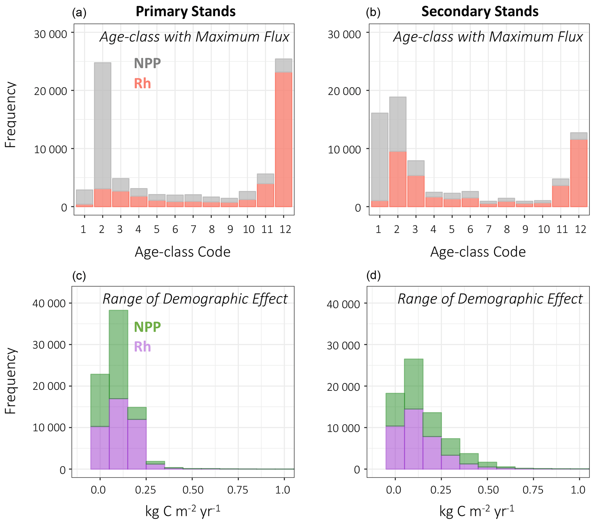
Figure 12Stacked frequency plots for NPP and Rh on primary and secondary stands. (a, b) Global frequency of age classes with the largest flux (NPP, Rh) relative to other age classes in the grid cell. Age-class codes, lowest (youngest) to greatest (oldest), correspond to the 10-yr-equalbin age-class setup (Table 1). (c, d) Global frequency of the range of the demographic effect on fluxes; bin width is 0.10 kg C m−2 yr−1. An example interpretation, on primary stands: (a) NPP is greatest in the second age class, and (c) the demographic effect on NPP is <0.25 kg C m−2 yr−1.
3.4.3 Frequency distribution of demographic effects
The global mean demographic effect on NPP on primary stands was 0.078±0.063 [0, 1.37] kg C m−2 yr−1 (μ±SD [min, max]), whereas on secondary stands it was 0.160±0.141 [0, 1.33] kg C m−2 yr−1. There were differences in the spatial distribution of primary and secondary stands that led to the disparity in global mean values of the demographic effect. On primary stands, the distribution of age classes with maximum NPP flux was skewed towards the second (11–20 years) age class having the maximum NPP flux, whereas on secondary stands, the maximum NPP flux was in the first (1–10 years) and also in the second age class (Fig. 12). The first class was categorized as 1–10 years, but in the presence of constant renewal, an age class can effectively be younger than an equivalent age class without such recurrent disturbance. Furthermore, on primary stands, fire is the only mechanism that creates young age classes, whereas land management also creates young age classes on secondary stands. It is possible for wood harvest, a form of simulated land management, to result in advanced regeneration of younger stands if harvest demand is met without “clear-cutting” the prescribed fractional area under harvest. Currently, the model structure does not lend itself to say definitively the cause of the difference in the age class of maximum flux, but the only process that differs between primary and secondary stands is land management, so it is reasonable to assume that land management is the cause of the difference. In any manner, global values for age effects for NPP on primary and secondary stands were also skewed towards greater values on secondary stands but more due to the absence of primary stands in productive areas where secondary stands dominated (e.g., eastern US).
Following a similar pattern, the demographic effects on Rh were greater on secondary stands than on primary stands (Figs. 11 and 12), which could be partly explained by the differential coverage of secondary and primary stands but also by historical land use. LUCLM leads to overall greater inputs to soil and litter carbon pools than does fire, and the latter is simulated in the same manner on secondary stands as on primary stands. In LPJ, wood harvest is only 60 % efficient, leaving dead biomass “residue” as a legacy flux. An increase of carbon in the litter and soil pools would add additional mass that can be respired during heterotrophic respiration and which manifests as a larger demographic effect on Rh, ranging from 0.25 to 0.70 kg C m−2 yr−1 on the high end (Fig. 12).
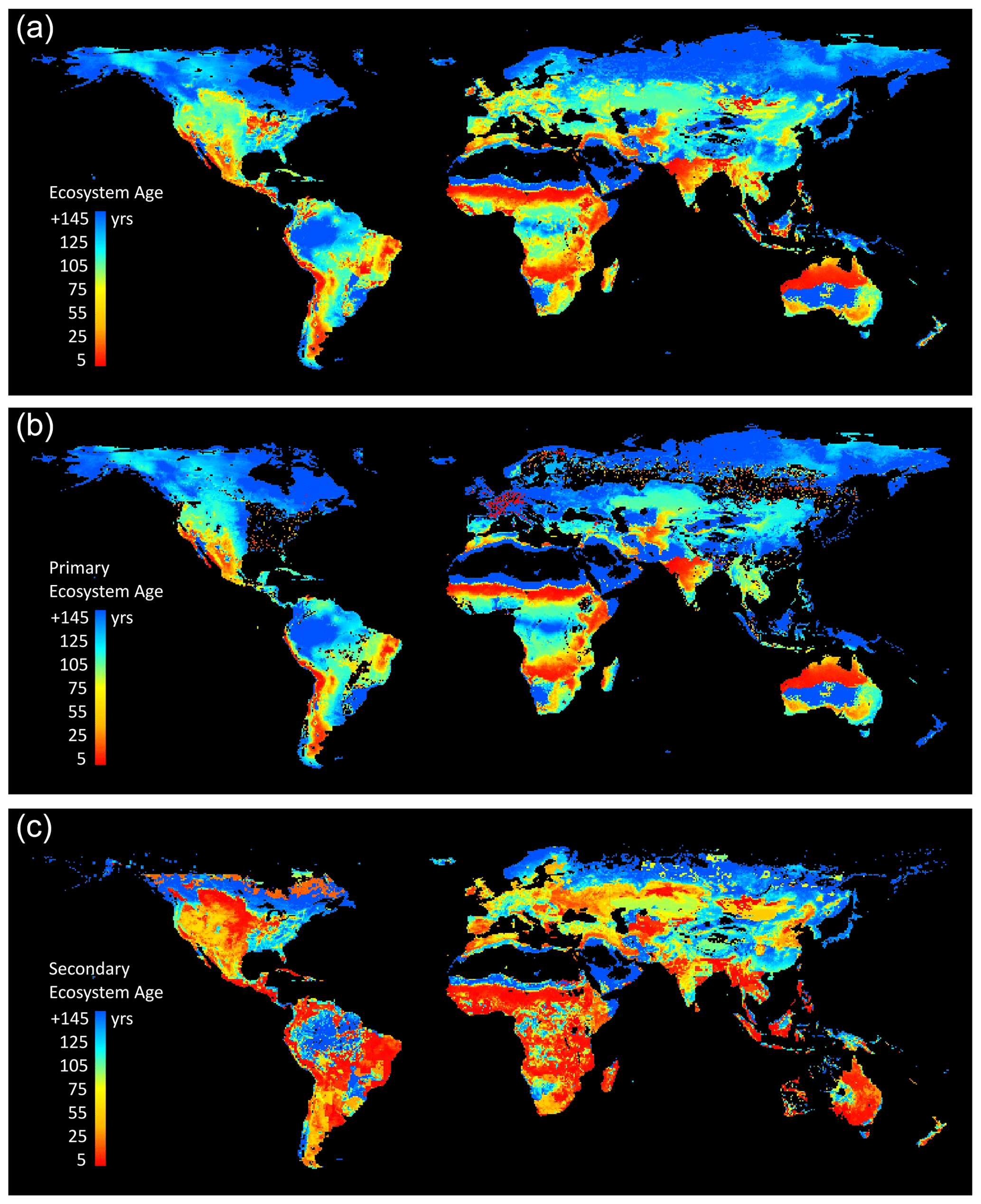
Figure 13LPJ-wsl v2.0 simulated global distribution of ecosystem ages, defined as the time since disturbance by fire and/or LUCLM in the year 2016. (a) Average age of the natural ecosystem, scaled to the area of natural lands within 0.5∘ grid cells. (b) Average age of primary ecosystems only, wherein only fire creates age structure, scaled to the area of primary lands. (c) Average age of secondary ecosystems only, wherein fire and LUCLM create age structure, scaled to the area of secondary lands.
4.1 Distribution of ecosystem age on Earth
The LPJ-wsl v2.0 age module simulates the age-class distributions on Earth resulting from fire, land-use change, and wood harvest (Fig. 13), while also simulating important demographics effects on NPP and Rh. Simulations demonstrate that fire and LUCLM have been driving the latitudinal age distribution towards younger states in contemporary times (Fig. 8), suggesting an increasing role of age dynamics in global ecosystem functioning. Whereas time is the only mechanism that increases ecosystem age, any additional disturbance not explicitly modeled in this study will decrease age.
The simulations omit widespread disturbances of windstorms, flood, pest and disease outbreak, selective logging, and other processes that would modify stand structure and function. For instance, small-scale logging activity is a dominant disturbance in the southeastern US (Williams et al., 2016) but it is underestimated by the LUCLM driver data in this study (LUHv2; Hurtt et al., 2020); otherwise, the simulated age of secondary forests in this region (∼100 years) would be lower and closer to inventory-based age estimates of these forests (<50 years; Fig. 4 in Pan et al., 2011b). In some geographic locations, it is certainly possible that our wood harvest priority rules (defined by harvesting oldest age class first) might lead to simulated stand ages that are younger than observed stand ages if other harvest rules were applied in real life. For example, if there are mandates to preserve old-growth forests, then logging might preferentially occur on young or mid-aged forests, leaving older-age-class forests unharvested. We evaluated the age distribution by continent simulated by LPJ-wsl v2.0 to the Global Forest Age Database (GFAD v1.0; Poulter et al., 2018), which is derived from country-level inventory data. The comparison shows that the simulated ages are consistently older than the GFAD dataset (Supplement Fig. S11). Furthermore, the fire module has been well evaluated at global scale (Thonicke et al., 2001) but it needs improvement because it is overly simplistic and underestimates global burned area (Hantson et al., 2020). It is more likely that effects of fire are much greater than those simulated in this study. This study likely underestimates disturbances rather than overestimates them, and as such, these simulations overestimate ecosystem age. But again, additional disturbances would only lead to younger age classes, enhancing the role of age dynamics in regional and global carbon cycles.
Our model developments are not optimized to match observations, although we are working toward this end. Future goals are to assimilate stand-age-related data, such as remotely sensed canopy data and stand index growth curves, to align model processes with observations. Even with these caveats in mind, the findings presented retain utility as insight into the way age-class dynamics integrate into our broader understanding of global carbon dynamics. Ecosystem demographics likely play a larger role than suggested here, and on regional scales, demographic effects on NPP and Rh are already identified by this study as more important in East Asia, tropical Asia, Europe, central Africa, eastern North America, and tropical South America than they are in other regions, where average ecosystem ages are much older.
4.2 Age dynamics increase turnover
In an analysis by Friend et al. (2014), it was determined that demographic processes (age-dependent mortality and turnover) influence carbon residence time, which was found to be a major source of uncertainty in future projections by global ecosystem models. In this study, it was demonstrated that simulation of age classes led to a ∼40 Pg C shift from live vegetation to the soil-litter pool, effectively an increase in biomass turnover. That turnover increases when explicitly simulating age classes is a natural expectation, but the magnitude of the simulated turnover between carbon pools less certain until detailed benchmarking is conducted. Further, relaxation times, or the time to return to a previous state, were up to 30 years in the no-age simulation (Snoage_event; Fig. 5) but relaxation times were less than 10 years when simulating age classes, suggesting that uncertainty in carbon residence time could potentially be reduced by improving representation of demographics in models. Omitting age-class representation in models can leave long-lasting patterns in simulated fluxes that could inflate land-use change fluxes at global scales when considering legacy fluxes from past land-use change (Pongratz et al., 2014). The current state of knowledge is that fluxes from gross land-use change and land management cause greater-than-expected land-use fluxes (Arneth et al., 2017), but existing models that estimate the global land-use flux (Arneth et al., 2017; Le Quéré et al., 2018) do not include age dynamics. If resiliency is inversely proportional to relaxation times (a quicker return to previous states is represented by shorter relaxation times and therefore greater resiliency; Pimm, 1984; Tilman and Downing, 1994), then instead of land-use change fluxes being “greater than assumed” (Arneth et al., 2017), we might rethink the land as being “more resilient than expected” when demographic effects are considered at large scales.
4.3 Forecasting demographic effects with a simplified statistical model
The modeling community has made increasing effort to simplify complex models using a traceability framework (Friedlingstein et al., 2006; Xia et al., 2013). Statistical emulators, from matrix models (Huang et al., 2018) to accounting-type statistical models, which track individual carbon pools (Xia et al., 2013; Ahlström et al., 2015b), have been developed to reduce the dimensionality of simulated state variables. However, statistical modeling by linear regression can be a more straightforward approach, as long as the statistical model shows promise.
We found that LPJ-wsl v2.0 fluxes of NPP and Rh could be predicted at annual timescales by three terms: precipitation, temperature, and age class. Part of the success of the data model came from allowing coefficients to vary by grid cell. This allowed the intercept (age-class) term to effectively capture grid cell level variation in soil texture (which influences soil hydrology and plant-available water), PFT composition, and cloud cover. Another insight was that climate and age class had differential effects on NPP versus Rh, which makes sense and ultimately led to poorer fit of the NEP model (NEP is the difference between NPP and Rh). It might have been possible to improve upon the NPP model further by separately modeling GPP and autotrophic respiration (NPP is the difference between GPP and Ra) because climate might also have differential effects on GPP than on Ra but suffice to say that the NPP statistical model was robust.
Although unexplored in this study, the spatial datasets of predictor coefficients could be used within an emulator (Xia et al., 2013; Ahlström et al., 2015a) to forecast NPP and Rh, while exploring the effects of extreme climate scenarios (Reichstein et al., 2013) and changes in ecosystem demography from land-use change and land management. Such application would allow for a much quicker exploration of scenarios and could include a more explicit treatment of uncertainty that would otherwise be too costly for the simulation model in terms of computing time. With regards to climate, the spatial dataset of precipitation coefficients has an equivalent meaning to spatial maps of climatic sensitivity. In fact, the maps of the effective range of precipitation on NPP (Fig. 11) show areas where the precipitation effect is largest, notably in semi-arid biomes – a biome that is known to be highly sensitive to precipitation and has been shown to play an important role in the interannual variability of global-scale fluxes (Poulter et al., 2014; Ahlström et al., 2015a). But what if, in a given year, semi-arid biomes received their maximum annual precipitation, while every other biome received its lowest annual precipitation – can anomalously high annual precipitation and high-productivity events in some regions overcome anomalously low-precipitation and low-productivity events in other regions? Are the effects of different climate scenarios dependent on demography? These types of question are best suited for exploration within a simplified statistical model that maintains fidelity to the process-based model because effects of climate on fluxes can be explored quicker, easier, and with a better treatment of statistical uncertainty.
A last note on emulators. Useful statistical emulators have fidelity to the underlying process model, but such emulators often cannot address uncertainty from parameter values that are often fixed in the underlying process model or uncertainty in process representation. In an ideal world, the statistical parameters for climate sensitivity and stand age, for instance, would be constrained by uncertainty simulations that are themselves bounded to a realistic range of parameter values in the process model (Zaehle et al., 2005) and alternate representations of ecosystem processes (Forkel et al., 2016).
4.4 VTFT – modeling age classes in global models
The VTFT approach simulated classic demographic responses in NPP and Rh (Fig. 4), a differential in younger age classes that led to a larger carbon sink in the youngest stands. These demographic responses are inherent within the original formulation in LPJ; that is, establishment rates and the process of self-thinning of stand density over time as plants grow and compete (for space, light, water resources) have been unchanged. In the original formulation of LPJ-wsl v2.0 (prior to this study), and under a hypothetical scenario where a disturbance clears the biomass from the entire grid cell (0.5∘ ∼2500 km2), the resultant evolution of stand structure and fluxes would produce the same pattern as in the age module, such as the age–NPP pattern from Fig. 4. It is often the case, however, that smaller disturbances (≪2500 km2) occur regularly as opposed to a much larger disturbance the size of the entire grid cell. As such, in the original formulation of LPJ, the potential benefits of demographic responses are often masked (as demonstrated in Sect. 3.2.2; Fig. 5). One can then say that the VTFT age module reveals intrinsic demographic responses and model behavior that would rarely emerge otherwise.
Total runtime for global age-class simulations (Sage) was ∼8 h on 32 Intel Xeon CPUs, including spinup to transient simulations, whereas the total runtime for the no-age simulations (Snoage) was ∼3 h. On a limited sample of single-grid-cell simulations, there was a 4- to 6-fold increase in runtime, but not all grid cells require simultaneous tracking of every age class so the increase in runtime of global simulations was lower than expected from per-grid-cell estimates.
4.5 Opportunities for improving modeled age dynamics
The order of priority for improvement of the age module is to (1) improve age-class growth rates to align with observations, (2) improve representation of disturbances, and (3) improve representation of early- and late-successional plant species and add vertical structural complexity such as understory/overstory canopy. Below, we provide suggestions and examples from the literature as how these improvements might be accomplished.
Inventory data or remotely sensed observations of canopy height provide a potential means for constructing age-height curves (Croft et al., 2014; Yue et al., 2016) to inform growth rates by age class. Alternately, Hiltner et al. (2020) recently optimized mortality rates in an individual-based model at different forest successional stages by using satellite-derived proxies of tree mortality (Hiltner et al., 2020); their optimized model was shown to improve representation of forest states during post-disturbance regrowth. Another LPJ variant, the LPJmL4 DGVM, also underwent parameter optimization to improve spatial patterns of tree cover and forest turnover (Forkel et al., 2019). Different solutions are possible, and not all of them require parameter optimization, but the aim should be to align simulated forest structure and function with observations.
Our comparison of simulated versus inventory forest age distributions by continent (Supplement Fig. S11) clearly show that LPJ-wsl v2.0 overestimates stand age. A potential solution to this discrepancy is to incorporate additional disturbances within the model to help simulate age distributions more consistent with inventory (Pan et al., 2011a) and satellite (Pugh et al., 2019a) data and contribute to more scientifically relevant questions. Firstly, general improvement of the fire module in LPJ-wsl v2.0 is necessary to match burned area observations. One such solution is to use a suite of satellite data products to prescribe burned area instead of simulating fire, which could help improve simulated stand age distributions in areas where fire is observed but not well simulated mechanistically (Poulter et al., 2015). Modeled disturbances need not be complex to explore their effects on age distributions, they only need to reset a fractional area to the youngest age class. For example, windstorms from hurricanes are known to be a large disturbance of eastern North American forests (Dale et al., 2001). Data on hurricane return intervals and locations of landfall in eastern North America have been available for some time (Keim et al., 2007) and could be used to prescribe a periodic resetting of age classes to assess the demographic effect of hurricanes on ecosystem function. In another example, forest gaps represent areas of high production because of high resource abundance relative to the surrounding areas. The distribution of forest gaps also has a predictable power-law relationship with size of the gap (Asner et al., 2013), which can be allowed to vary across and within regions (Asner et al., 2013; Espírito-Santo et al., 2014), and this fact lends itself well to representing gaps within the framework of the current age module. Many disturbances can be prescribed based on observed forest disturbance rates (Pugh et al., 2019a), but prescribed disturbance patterns typically sacrifice capacity to simulate under novel conditions so there are tradeoffs to consider.
There are limitations to the current framework of the model, which are more difficult to overcome and will require more effort in model development. In this version of the model, plant composition, and competitive dynamics in young age classes are not representative of early successional dynamics because there is a lack of plant trait variation in the current set of PFTs that could otherwise represent a wider range of growth strategies, turnover, and production (Pütz et al., 2011; Fisher et al., 2016; Miller et al., 2016). There is also no height variation within an age class, for lack of a radiative transfer model; each age class in LPJ-wsl v2.0 is an even-height stand. Demographic patterns in this study (age–NPP, age–Rh, relaxation times by age class) will inevitably differ when, and if, additional trait and height variations are incorporated into the model. Recent model developments in JSBACH4 (Nabel et al., 2020) and ED-2.2 (Longo et al., 2019) could point at a way forward for incorporating a greater amount of vertical heterogeneity in LPJ-wsl v2.0, as well as in other models.
LPJ-wsl v2.0 model code, in its entirety, is freely available at https://github.com/benpoulter/LPJ-wsl_v2.0 (last access: 28 July 2020), and a permanent version of the model code is deposited at Zenodo, https://doi.org/10.5281/zenodo.4409331 (Calle and Poulter, 2021). Code used for analyses and figure production are available at https://github.com/lcalle/VTFT_demography (last access: 28 July 2020). Associated data necessary to reproduce the analyses and figures, as well as a copy of the analysis code, are permanently archived at the Dryad Digital Repository https://doi.org/10.5061/dryad.k6djh9w4x (Calle, 2020).
The supplement related to this article is available online at: https://doi.org/10.5194/gmd-14-2575-2021-supplement.
LC and BP designed the model experiments and LC carried them out. LC developed the code for the age-class module and performed the simulations. LC and BP prepared the manuscript.
The authors declare that they have no conflict of interest.
Computational efforts were performed on the Hyalite High Performance Computing System, operated and supported by University Information Technology Research Cyberinfrastructure at Montana State University. Leonardo Calle was supported by a National Aeronautics and Space Administration Earth and Space Science Fellowship (NASA ESSF 2016-2019, grant no. NNX16AP86H). This work contributed to the 3DSI Project (NASA proposal no. 16-CARBON16-0124). The authors thank Paul Montesano, Bryce Currey, and Tom Pugh for comments on the manuscript.
This research has been supported by the US National Aeronautics and Space Administration (NASA) (grant no. NNX16AP86H).
This paper was edited by Christoph Müller and reviewed by three anonymous referees.
Ahlström, A., Raupach, M. R., Schurgers, G., Smith, B., Arneth, A., Jung, M., Reichstein, M., Canadell, J. G., Friedlingstein, P., Jain, A. K., Kato, E., Poulter, B., Sitch, S., Stocker, B. D., Viovy, N., Wang, Y. P., Wiltshire, A., Zaehle, S., and Zeng, N.: The dominant role of semi-arid ecosystems in the trend and variability of the land CO2 sink, Science, 348, 895–898, https://doi.org/10.1126/science.aaa1668, 2015a.
Ahlström, A., Xia, J., Arneth, A., Luo, Y., and Smith, B.: Importance of vegetation dynamics for future terrestrial carbon cycling, Environ. Res. Lett., 10, 5, https://doi.org/10.1088/1748-9326/10/5/054019, 2015b.
Arneth, A., Sitch, S., J. Pongratz, Stocker, B. D., Ciais, P., Poulter, B., Bayer, A. D., Bondeau, A., Calle, L., Chini, L. P., Gasser, T., Fader, M., Friedlingstein, P., Kato, E., Li, W., Lindeskog, M., Nabel, J. E. M. S., Pugh, T. A. M., Robertson, E., Viovy, N., Yue, C., and Zaehle, S.: Historical carbon dioxide emissions caused by land-use changes are possibly larger than assumed, Nat. Geosci., 10, 79–84, https://doi.org/10.1038/NGEO2882, 2017.
Asner, G. P., Kellner, J. R., Kennedy-Bowdoin, T., Knapp, D. E., Anderson, C., and Martin, R. E.: Forest canopy gap distributions in the Southern Peruvian Amazon, PLoS ONE, 8, e60875, https://doi.org/10.1371/journal.pone.0060875, 2013.
Bondeau, A., Smith, P. C., Zaehle, S., Schaphoff, S., Lucht, W., Cramer, W., Gerten, D., Lotze-Campen, H., Müller, C., Reichstein, M., and Smith, B.: Modelling the role of agriculture for the 20thcentury global terrestrial carbon balance, Global Change Biol., 13, 679–706, 2007.
Box, E. O.: Plant functional types and climate at the global scale, J. Vegetat. Sci., 7, 309–320, 1996.
Calle, L.: VTFT_Demography: global ageclass simulation data from the LPJ-wsl v2.0 Dynamic Global Vegetation Model, Dryad, dataset, https://doi.org/10.5061/dryad.k6djh9w4x, 2020.
Calle, L. and Poulter, B.: Model code for the LPJ-wsl_v2.0 Dynamic Global Vegetation Model, Zenodo, https://doi.org/10.5281/zenodo.4409331, 2021.
Croft, H., Chen, J. M., and Noland, T. L.: Stand age effects on Boreal forest physiology using a long time-series of satellite data, Forest Ecol. Manage., 328, 202–208, https://doi.org/10.1016/j.foreco.2014.05.023, 2014.
Dale, V. H., Joyce, L. A., McNulty, S., Neilson, R. P., Ayres, M. P., Flannigan, M. D., Hanson, P. J., Irland, L. C., Lugo, A. E., Peterson, C. J., Simberloff, D., Swanson, F. J., Stocks, B. J., and Wotton, B. M.: Climate change and forest disturbance, BioScience, 51, 723–734, 2001.
Drake, J. E., Raetz, L. M., Davis, S. C., and DeLucia, E. H.: Hydraulic limitation not declining nitrogen availability causes the age-related photosynthetic decline in loblolly pine (Pinus taeda L.), Plant Cell Environ., 33, 1756–1766, https://doi.org/10.1111/j.1365-3040.2010.02180.x, 2010.
Drake, J. E., Davis, S. C., Raetz, L. M., and DeLucia, E. H.: Mechanisms of age-related changes in forest production: the influence of physiological and successional changes, Global Change Biol., 17, 1522–1535, https://doi.org/10.1111/j.1365-2486.2010.02342.x, 2011.
Earles, J. M., Yeh, S., and Skog, K. E.: Timing of carbon emissions from global forest clearance, Nat. Clim. Change, 2, 682–685, https://doi.org/10.1038/NCLIMATE1535, 2012.
Espírito-Santo F. D. B., Gloor M., Keller, M., Malhi, Y., Saatchi, S., Nelson, B., Oliveira Junior, R. C., Pereira, C., Lloyd, J., Frolking, S., Palace, M., Shimabukuro, Y. E., Duarte, V., Mendoza, A. M., López-González, G., Baker, T. R., Feldpausch, T. R., Brienen, R. J. W., Asner, G. P., Boyd, D. S., and Phillips, O. L.: Size and frequency of natural forest disturbances and the Amazon forest carbon balance, Nat. Commun., 5, 3434, https://doi.org/10.1038/ncomms4434, 2014.
Eyring, V., Bony, S., Meehl, G. A., Senior, C. A., Stevens, B., Stouffer, R. J., and Taylor, K. E.: Overview of the Coupled Model Intercomparison Project Phase 6 (CMIP6) experimental design and organization, Geosci. Model Dev., 9, 1937–1958, https://doi.org/10.5194/gmd-9-1937-2016, 2016.
FAO-FRA: U.N. Food and Agriculture Organization, Forest Resource Assessment, Rome, Italy, 2015.
Farquhar, G. D., von Caemmerer, S., and Berry, J. A.: A biochemical model of photosynthetic CO2 assimilation in leaves of C3 plants, Planta, 149, 78–90, 1980.
Fisher, R., Bohn, F., de Paula, M. D., Dislich, C., Groeneveld, J., Gutiérrez, A. G., Kazmierczak, M., Knapp, N., Lehmann, S., Paulick, S., Pütz, S., Rödig, E., Taubert, F., Köhler, P., and Huth, A.: Lessons learned from applying a forest gap model to understand ecosystem and carbon dynamics of complex tropical forests, Ecol. Model., 326, 124–133, https://doi.org/10.1016/j.ecolmodel.2015.11.018, 2016.
Forkel, M., Carvalhais, N., Rödenbeck, C., Keeling, R., Heimann, M., Thonicke, K., Zaehle, S., and Reichstein, M.: Enhanced seasonal CO2 exchange caused by amplified plant productivity in northern ecosystems, Science, 351, 696–699, https://doi.org/10.1126/science.aac4971, 2016.
Forkel, M., Drüke, M., Thurner, M., Dorigo, W., Schaphoff, S., Thonicke, K., von Blog, W., and Carvalhais, N.: Constraining modelled global vegetation dynamics and carbon turnover using multiple satellite observations, Sci. Rep.-UK, 9, 18757, https://doi.org/10.1038/s41598-019-55187-7, 2019.
Friedlingstein, P., Cox, P., Betts, R., Bopp, L., von Bloh, W., Brovkin, V., Cadule, P., Doney, S., Eby, M., Fung, I., Bala, G., John, J., Jones, C., Joos, F., Kato, T., Kawamiya, M., Knorr, W., Lindsay, K., Matthews, H. D., Raddatz, T., Rayner, P., Reick, C., Roeckner, E., Schnitzler, K.-G., Schnur, R., Strassmann, K., Weaver, A. J., Yoshikawa, C., and Zeng, N.: Climate-carbon cycle feedback analysis: Results from the C4MIP Model Intercomparison, J. Climate, 19, 3337–3353, 2006.
Friend, A. D., Lucht, W., Rademacher, T. T., Keribin, R., Betts, R., Cadule, P., Ciais, P., Clark, D. B., Dankers, R., Falloon, P. D., Ito, A., Kahana, R., Kleidon, A., Lomas, M. R., Nishina, K., Ostberg, S., Pavlick, R., Peylin, P., Schaphoff, S., Vuichard, N., Warszawski, Wiltshire, A., and Woodward, F. I.: Carbon residence time dominates uncertainty in terrestrial vegetation responses to future climate and atmospheric CO2, P. Natl. Acad. Sci. USA, 111, 3280–3285, https://doi.org/10.1073/pnas.1222477110, 2014.
Frolking, S., Palace, M. W., Clark, D. B., Chambers, J. Q., Shugart, H. H., and Hurtt, G. C.: Forest disturbance and recovery: A general review in the context of spaceborne remote sensing of impacts on aboveground biomass and canopy structure, J. Geophys. Res., 114, G00E02, https://doi.org/10.1029/2008JG000911, 2009.
Gitz, V. and Ciais, P.: Amplifying effects of land-use change on future atmospheric CO2 levels, Global Biogeochem. Cycles, 17, 1024, https://doi.org/10.1029/2002GB001963, 2003.
Goldewijk, K. K.: Estimating global land use change over the past 300 years: The HYDE Database, Global Biogeochem. Cycles, 15, 417–433, 2001.
Hantson, S., Kelley, D. I., Arneth, A., Harrison, S. P., Archibald, S., Bachelet, D., Forrest, M., Hickler, T., Lasslop, G., Li, F., Mangeon, S., Melton, J. R., Nieradzik, L., Rabin, S. S., Prentice, I. C., Sheehan, T., Sitch, S., Teckentrup, L., Voulgarakis, A., and Yue, C.: Quantitative assessment of fire and vegetation properties in simulations with fire-enabled vegetation models from the Fire Model Intercomparison Project, Geosci. Model Dev., 13, 3299–3318, https://doi.org/10.5194/gmd-13-3299-2020, 2020.
Haxeltine, A. and Prentice, I. C.: A general model for the light-use efficiency of primary production, Funct. Ecol., 10, 551–561, 1996.
Haverd, V., Smith, B., Nieradzik, L. P., and Briggs, P. R.: A stand-alone tree demography and landscape structure module for Earth system models: integration with inventory data from temperate and boreal forests, Biogeosciences, 11, 4039–4055, https://doi.org/10.5194/bg-11-4039-2014, 2014.
Hiltner, U., Huth, A., and Fischer, R.: Importance of succession in estimating biomass loss: Combining remote sensing and individual-based forest models, Biogeosciences Discuss. [preprint], https://doi.org/10.5194/bg-2020-264, 2020.
Houghton, R. A.: The annual net flux of carbon to the atmosphere from changes in land use 1850–1990, Tellus B, 51B, 298–313, 1999.
Huang, Y., Lu, X., Shi, Z., Lawrence, D., Koven, C. D., Xia, J., Du, Z., Kluzek, E., and Luo, Y.: Matrix approach to land carbon cycle modeling: A case study with the Community Land Model, Global Change Biol., 24, 1394–1404, https://doi.org/10.1111/gcb.13948, 2018.
Hurtt, G. C., Frolking, S., Fearon, M. G., Moore, B., Shevliakova, E., Malyshev, S., Pacala, S. W., and Houghton, R. A.: The underpinnings of land-use history: three centuries of global gridded land-use transitions, wood-harvest activity, and resulting secondary lands, Global Change Biol., 12, 1208–1229, https://doi.org/10.1111/j.1365-2486.2006.01150.x, 2006.
Hurtt, G. C., Chini, L. P., Frolking, S., Betts, R. A., Feddema, J., Fischer, G., Fisk, J. P., Hibbard, K., Houghton, R. A., Janetos, A., Jones, C. D., Kindermann, G., Kinoshita, T., Goldewijk, K. K., Riahi, K., Shevliakova, E., Smith, S., Stehfest, E., Thomson, A., Thornton, P., van Vuuren, D. P., and Wang, Y. P.: Harmonization of land-use scenarios for the period 1500–2100: 600 years of global gridded annual land-use transitions, wood harvest, and resulting secondary lands, Clim. Change, 109, 117–161, https://doi.org/10.1007/s10584-011-0153-2, 2011.
Hurtt, G. C., Chini, L., Sahajpal, R., Frolking, S., Bodirsky, B. L., Calvin, K., Doelman, J. C., Fisk, J., Fujimori, S., Klein Goldewijk, K., Hasegawa, T., Havlik, P., Heinimann, A., Humpenöder, F., Jungclaus, J., Kaplan, J. O., Kennedy, J., Krisztin, T., Lawrence, D., Lawrence, P., Ma, L., Mertz, O., Pongratz, J., Popp, A., Poulter, B., Riahi, K., Shevliakova, E., Stehfest, E., Thornton, P., Tubiello, F. N., van Vuuren, D. P., and Zhang, X.: Harmonization of global land use change and management for the period 850–2100 (LUH2) for CMIP6, Geosci. Model Dev., 13, 5425–5464, https://doi.org/10.5194/gmd-13-5425-2020, 2020.
Keim, B. D., Muller, R. A., and Stone, G. W.: Spatiotemporal patterns and return periods of tropical storm and hurricane strikes from Texas to Maine, J. Climate, 20, 3498–3509, https://doi.org/10.1175/JCLI4187.1, 2007.
Kondo, M., Ichii, K., Patra, P. K., Poulter, B., Calle, L., Koven, C., Pugh, T. A. M., Kato, E., Harper, A., Zaehle, S., and Wiltshire, A.: Plant regrowth as a driver of recent enhancement of terrestrial CO2 uptake, Geophys. Res. Lett., 45, 4820–4830, https://doi.org/10.1029/2018GL077633, 2018.
Lawrence, D. M., Fisher, R. A., Koven, C. D., Oleson, K. W., Swenson, S. C., Vertenstein, M., Andre, B., Bonan, G., Ghimire, B., van Kampenhout, L., Kennedy, D., Kluzek, E., Knox, R., Lawrence, P. J., Li, F., Li, H., Lombardozzi, D., Lu, Y., Perket, J., Riley, W. J. Sacks, W. J., Shi, M., Wieder, W. R., Xu, C., Ali, A., Badger, A., Bisht, G., Broxton, P., Brunke, M., Buzan, J., Clark, M., Craig, A., Dahlin, K., Drewniak, B., Fisher, J. B., Flanner, M., Gentine, P., Lenaerts, J., Levis, S., Leung, L. R., Lipscomb, W. H., Pelletier, J. D., T., Ricciuto, D. M., Sanderson, B. M., Shuman, J., Slater, A., Subin, Z., Tang, J., Tawfik, A., Thomas, R. Q., Tilmes, S., Vitt, F., and Zeng, X.: Technical description of version 5.0 of the Community Land Model (CLM), The National Center for Atmospheric Research, Boulder, CO, 2019.
Le Quéré, C., Andrew, R. M., Friedlingstein, P., Sitch, S., Pongratz, J., Manning, A. C., Korsbakken, J. I., Peters, G. P., Canadell, J. G., Jackson, R. B., Boden, T. A., Tans, P. P., Andrews, O. D., Arora, V. K., Bakker, D. C. E., Barbero, L., Becker, M., Betts, R. A., Bopp, L., Chevallier, F., Chini, L. P., Ciais, P., Cosca, C. E., Cross, J., Currie, K., Gasser, T., Harris, I., Hauck, J., Haverd, V., Houghton, R. A., Hunt, C. W., Hurtt, G., Ilyina, T., Jain, A. K., Kato, E., Kautz, M., Keeling, R. F., Klein Goldewijk, K., Körtzinger, A., Landschützer, P., Lefèvre, N., Lenton, A., Lienert, S., Lima, I., Lombardozzi, D., Metzl, N., Millero, F., Monteiro, P. M. S., Munro, D. R., Nabel, J. E. M. S., Nakaoka, S., Nojiri, Y., Padin, X. A., Peregon, A., Pfeil, B., Pierrot, D., Poulter, B., Rehder, G., Reimer, J., Rödenbeck, C., Schwinger, J., Séférian, R., Skjelvan, I., Stocker, B. D., Tian, H., Tilbrook, B., Tubiello, F. N., van der Laan-Luijkx, I. T., van der Werf, G. R., van Heuven, S., Viovy, N., Vuichard, N., Walker, A. P., Watson, A. J., Wiltshire, A. J., Zaehle, S., and Zhu, D.: Global Carbon Budget 2017, Earth Syst. Sci. Data, 10, 405–448, https://doi.org/10.5194/essd-10-405-2018, 2018.
Lindeskog, M., Arneth, A., Bondeau, A., Waha, K., Seaquist, J., Olin, S., and Smith, B.: Implications of accounting for land use in simulations of ecosystem carbon cycling in Africa, Earth Syst. Dynam., 4, 385–407, https://doi.org/10.5194/esd-4-385-2013, 2013.
Longo, M., Knox, R. G., Medvigy, D. M., Levine, N. M., Dietze, M. C., Kim, Y., Swann, A. L. S., Zhang, K., Rollinson, C. R., Bras, R. L., Wofsy, S. C., and Moorcroft, P. R.: The biophysics, ecology, and biogeochemistry of functionally diverse, vertically and horizontally heterogeneous ecosystems: the Ecosystem Demography model, version 2.2 – Part 1: Model description, Geosci. Model Dev., 12, 4309–4346, https://doi.org/10.5194/gmd-12-4309-2019, 2019.
McGuire, A. D., Sitch, S., Clein, J. S., Dargaville, R., Esser, G., Foley, J., Heimann, M., Joos, F., Kaplan, J., Kicklighter, D. W., Meier, R. A., Melillo, J. M., Moore III, B., Prentice, I. C., Ramankutty, N., Reichenau, T., Schloss, A., Tian, H., Williams, L. J., and Wittenberg, U.: Carbon balance of the terrestrial biosphere in the twentieth century: Analyses of CO2, climate and land use effects with four process-based ecosystem models, Global Biogeochem. Cycles, 15, 183–206, 2001.
Medvigy, D., Wofsy, S. C., Munger, J. W., Hollinger, D. Y., and Moorcroft, P. R.: Mechanistic scaling of ecosystem function and dynamics in space and time: Ecosystem Demography model version 2, J. Geophys. Res., 114, G01002, https://doi.org/10.1029/2008JG000812, 2009.
Miller, A. D., Dietze, M. C., DeLucia, E. H., and Anderson-Teixeira, K. J.: Alteration of forest succession and carbon cycling under elevated CO2, Global Change Biol., 22, 351–363, https://doi.org/10.1111/gcb.13077, 2016.
Nabel, J. E. M. S., Naudts, K., and Pongratz, J.: Accounting for forest age in the tile-based dynamic global vegetation model JSBACH4 (4.20p7; git feature/forests) – a land surface model for the ICON-ESM, Geosci. Model Dev., 13, 185–200, https://doi.org/10.5194/gmd-13-185-2020, 2020.
Nachtergaele, F., Van Velthuizen, H., Verelst, L., Batjes, N., Dijkshoorn, K., Van Engelen, V., Fischer, G., Jones, A., Montanarella, L., and Petri, M.: Harmonized world soil database, FAO, Rome, Italy and IIASA, Laxenburg, Austria, 2008.
O'Connell, B. M., LaPoint, E. B., Turner, J. A., Ridley, T., Pugh, S. A., Wilson, A. M., Waddell, K. L., and Conkling, B. L.: The Forest Inventory and Analysis Database: Database description and user guide version 6.0.2 for Phase 2, U.S. Department of Agriculture, Forest Service, 748 pp., available at: http://www.fia.fs.fed.us/library/databasedocumentation/ (last access: September 2019), 2015.
Odum, E. P.: The strategy of ecosystem development, Science, 164, 262–270, 1969.
Pan, Y., Birdsey, R. A., Fang, J., Houghton, R., Kauppi, P. E., Kurz, W. A., Phillips, O. L., Shvidenko, A., Lewis, S. L., Canadell, J. G., Ciais, P., Jackson, R. B., Pacala, S. W., McGuire, A. D., Piao, S., Rautiainen, A., Sitch, S., and Hayes, D.: A large and persistent carbon sink in the world's forests, Science, 333, 988–993, 2011a.
Pan, Y., Chen, J. M., Birdsey, R., McCullough, K., He, L., and Deng, F.: Age structure and disturbance legacy of North American forests, Biogeosciences, 8, 715–732, https://doi.org/10.5194/bg-8-715-2011, 2011b.
Pimm, S. L.: The complexity and stability of ecosystems, Nature, 307, 321–326, 1984.
Pongratz, J., Reick, C. H., Houghton, R. A., and House, J. I.: Terminology as a key uncertainty in net land use and land cover change carbon flux estimates, Earth Syst. Dynam., 5, 177–195, https://doi.org/10.5194/esd-5-177-2014, 2014.
Potter, C., Tan, P.-N., Steinbach, M., Klooster, S., Kumar, V., Myneni, R., and Genovese, V.: Major disturbance events in terrestrial ecosystems detected using global satellite data sets, Global Change Biol., 9, 1005–1021, 2003.
Poulter, B., Frank, D., Ciais, P., Myneni, R. B., Andela, N., Bi, J., Broquet, G., Canadell, J. G., Chevallier, F., Liu, Y. Y., Running, S. W., Sitch, S., and van der Werf, G. R.: Contribution of semi-arid ecosystems to interannual variability of the global carbon cycle, Nature, 509, 600–603, https://doi.org/10.1038/nature13376, 2014.
Poulter, B., Cadule, P., Cheiney, A., Ciais, P., Hodson, E., Peylin, P., Plummer, S., Spessa, A., Saatchi, S., Yue, C., and Zimmermann, N. E.: Sensitivity of global terrestrial carbon cycle dynamics to variability in satellite-observed burned area, Global Biogeochem. Cycles, 29.2, 207–222, 2015.
Poulter, B., Aragão, L., Andela, N., Bellassen, V., Ciais, P., Kato, T., Lin, X., Nachin, B., Luyssaert, S., Pederson, N., Peylin, P., Piao, S., Saatchi, S., Schepaschenko, D., Schelhaas, M., and Shivdenko, A.: The global forest age dataset (GFADv1.0), link to NetCDF file. NASA National Aeronautics and Space Administration, PANGAEA, https://doi.org/10.1594/PANGAEA.889943, 2018.
Pretzsch, H. and Biber, P.: A re-evaluation of Reineke's Rule and stand density index, Forest Sci., 51, 304–320, 2005.
Pretzsch, H., Grote, R., Reineking, B., Rötzer, T. H., and Seifert, S. T.: Models for Forest Ecosystem Mangement: A European Perspective, Ann. Bot., 101, 1065–1087, https://doi.org/10.1093/aob/mcm246, 2008.
Pugh, T. A. M., Arneth, A., Kautz, M., Poulter, B., and Smith, B.: Important role of forest disturbances in the global biomass turnover and carbon sinks, Nat. Geosci., 12, 730–735, https://doi.org/10.1038/s41561-019-0427-2, 2019a.
Pugh, T. A. M., Lineskog, M., Smith, B., Poulter, B., Arneth, A., Haverd, V., and Calle, L.: Role of forest regrowth in global carbon sink dynamics, P. Natl. Acad. Sci. USA, 116, 4382–4387, https://doi.org/10.1073/pnas.1810512116, 2019b.
Pütz, S., Groeneveld, J., Alves, L. F., Metzger, J. P., and Huth, A.: Fragmentation drives tropical forest fragments to early successional states: A modelling study for Brazilian Atlantic forests, Ecol. Model., 222, 1986–1997, https://doi.org/10.1016/j.ecolmodel.2011.03.038, 2011.
Reichstein, M., Bahn, M., Ciais, P., Frank, D., Mahecha, M. D., Seneviratne, S. I., Zscheischler, J., Beer, C., Buchmann, N., Frank, D. C., Papale, D., Rammig, A., Smith, P., Thonicke, K., van der Velde, M., Vicca, S., Walz, A., and Wattenbach, M.: Climate extremes and the carbon cycle, Nature, 500, 287–295, https://doi.org/10.1038/nature12350, 2013.
Ryan, M. G., Binkley, D., Fownes, J. H., Giardina, C. P., and Senock, R. S.: An experimental test of the causes of forest growth decline with stand age, Ecol. Monogr., 74, 393–414, 2004.
Schaphoff, S., von Bloh, W., Rammig, A., Thonicke, K., Biemans, H., Forkel, M., Gerten, D., Heinke, J., Jägermeyr, J., Knauer, J., Langerwisch, F., Lucht, W., Müller, C., Rolinski, S., and Waha, K.: LPJmL4 – a dynamic global vegetation model with managed land – Part 1: Model description, Geosci. Model Dev., 11, 1343–1375, https://doi.org/10.5194/gmd-11-1343-2018, 2018.
Shevliakova, E., Pacala, S. W., Malyshev, S., Hurtt, G. C., Milly, P. C. D., Caspersen, J. P., Sentman, L. T., Fisk, J. P., Wirth, C., and Crevoisier, C.: Carbon cycling under 300 years of land use change: Importance of the secondary vegetation sink, Global Biogeochem. Cycles, 23, GB2022, https://doi.org/10.1029/2007GB003176, 2009.
Sitch, S., Smith, B., Prentice, I. C., Arneth, A., Bondeau, A., Cramer, W., Kaplan, J. O., Levis, S., Lucht, W., Sykes, M. T., Thonicke, K., and Venevsky, S.: Evaluation of ecosystem dynamics, plant geography and terrestrial carbon cycling in the LPJ dynamic global vegetation model, Global Change Biol., 9, 161–185, 2003.
Stephenson, N. L., Das., A. J., Condit, R., Russo, S. E., Baker, P. J., Beckman, N. G., Coomes, D. A., Lines, E. R., Morris, W. K., Rüger, N., Alvarez, E., Blundo, C., Bunyavejchewin, S., Chuyong, G., Davies, S. J., Duque, A., Ewango, C. N., Flores, O., Franklin, J. F., Grau, H. R., Hao, Z., Harmon, M. E., Hubbell, S. P., Kenfack, D., Lin, Y., Makana, J.-R., Malizia, A., Malizia, L. R., Pabst, R. J., Pongpattananurak, N., Su, S.-H., Sun, I-F., Tan, S., Thomas, D., van Mantgem, P. J., Wang, X., Wiser, S. K., and Zavala, M. A.: Rate of tree carbon accumulation increases continuously with tree size, Nature, 507, 90–93, https://doi.org/10.1038/nature12914, 2014.
Stocker, B. D., Feissli, F., Strassmann, K. M., Spahni, R., and Joos, F.: Past and future carbon fluxes from land use change, shifting cultivation and wood harvest, Tellus B, 66, 23188, https://doi.org/10.3402/tellusb.v66.23188, 2014.
Thonicke, K., Venevsky, S., Sitch, S., and Cramer, W.: The role of fire disturbance for global vegetation dynamics: coupling fire into a Dynamic Global Vegetation Model, Global Ecol. Biogeogr., 10, 661–677, 2001.
Tilman, D. and Downing, J. A.: Biodiversity and stability in grasslands, Nature, 367, 363–365, 1994.
Turner, M. G.: Disturbance and landscape dynamics in a changing world, Ecology, 91, 2833–2849, 2010.
van der Werf, G. R., Randerson, J. T., Giglio, L., van Leeuwen, T. T., Chen, Y., Rogers, B. M., Mu, M., van Marle, M. J. E., Morton, D. C., Collatz, G. J., Yokelson, R. J., and Kasibhatla, P. S.: Global fire emissions estimates during 1997–2016, Earth Syst. Sci. Data, 9, 697–720, https://doi.org/10.5194/essd-9-697-2017, 2017.
Williams, C A., Gu, H., MacLean, R., Masek, J. G., and Collatz, G. J.: Disturbance and the carbon balance of US forests: A quantitative review of impacts from harvests, fires, insects, and droughts, Global Planet. Change, 143, 66–80, https://doi.org/10.1016/j.gloplacha.2016.06.002, 2016.
Xia, J., Luo, Y., Wang, Y.-P., and Hararuk, O.: Traceable components of terrestrial carbon storage capacity in biogeochemical models, Global Change Biol., 19, 2104–2116, 2013..
Yue, C., Kahle, H.-P., von Wilpert, K., and Kohnle, U.: A dynamic environment-sensitive site index model for the prediction of site productivity potential under climate change, Ecol. Model., 337, 48–62, https://doi.org/10.1016/j.ecolmodel.2016.06.005, 2016.
Yue, C., Ciais, P., Luyssaert, S., Li, W., McGrath, M. J., Chang, J., and Peng, S.: Representing anthropogenic gross land use change, wood harvest, and forest age dynamics in a global vegetation model ORCHIDEE-MICT v8.4.2, Geosci. Model Dev., 11, 409–428, https://doi.org/10.5194/gmd-11-409-2018, 2018.
Zaehle, S., Sitch, S., Smith, B., and Hatterman, F.: Effects of parameter uncertainties on the modeling of terrestrial biosphere dynamics, Global Biogeochem. Cycles, 19, GB3020, https://doi.org/10.1029/2004GB002395, 2005.
LPJ and LPJmL history; https://www.pik-potsdam.de/research/projects/activities/biosphere-water-modelling/lpjml/history-1 (last access: 28 July 2020).