the Creative Commons Attribution 4.0 License.
the Creative Commons Attribution 4.0 License.
 | 06 May 2021
WRF4PALM v1.0: a mesoscale dynamical driver for the microscale PALM model system 6.0
Dongqi Lin
Basit Khan
Marwan Katurji
Leroy Bird
Ricardo Faria
Laura E. Revell
A set of Python-based tools, WRF4PALM, has been developed for offline nesting of the PALM model system 6.0 into the Weather Research and Forecasting (WRF) modelling system. Time-dependent boundary conditions of the atmosphere are critical for accurate representation of microscale meteorological dynamics in high-resolution real-data simulations. WRF4PALM generates initial and boundary conditions from WRF outputs to provide time-varying meteorological forcing for PALM. The WRF model has been used across the atmospheric science community for a broad range of multidisciplinary applications. The PALM model system 6.0 is a turbulence-resolving large-eddy simulation model with an additional Reynolds-averaged Navier–Stokes (RANS) mode for atmospheric and oceanic boundary layer studies at microscale (Maronga et al., 2020). Currently PALM has the capability to ingest output from the regional scale Consortium for Small-scale Modelling (COSMO) atmospheric prediction model. However, COSMO is not an open source model and requires a licence agreement for operational use or academic research (http://www.cosmo-model.org/, last access: 23 April 2021). This paper describes and validates the new free and open-source WRF4PALM tools (available at https://github.com/dongqi-DQ/WRF4PALM, last access: 23 April 2021). Two case studies using WRF4PALM are presented for Christchurch, New Zealand, which demonstrate successful PALM simulations driven by meteorological forcing from WRF outputs. The WRF4PALM tools presented here can potentially be used for micro- and mesoscale studies worldwide, for example in boundary layer studies, air pollution dispersion modelling, wildfire emissions and spread, urban weather forecasting, and agricultural meteorology.
- Article
(12629 KB) - Full-text XML
-
Supplement
(23935 KB) - BibTeX
- EndNote


Over the last decade, research in numerical weather and climate simulations, environmental modelling, and agricultural and urban meteorology has developed to include higher spatial resolutions, such that the feedback from the microscale (from 10−2 to 103 m; from seconds to hours) processes impacted by surface heterogeneities can be explicitly resolved and better represented. At the mesoscale (from 104 to 5×10⁵ m; from hours to days), numerical weather prediction (NWP) models are widely used to simulate regional atmospheric flows in real meteorological conditions. Mesoscale NWP models are primarily Reynolds-averaged (Navier–Stokes) (RANS) simulation models that parameterise turbulence without discrepancy for scale (Sagaut, 2006, Chapter 1.4). The parameterisations applied in RANS models only consider the average properties of atmospheric flows impacted by surface geometries at the grid resolution of the simulation. In contrast to RANS models, large-eddy simulation (LES) models apply a local spatial filter to solve 3-D prognostic equations (Sagaut, 2006, Chapter 1.4). Eddies with scales smaller than the filter (sub-grid scales) are parameterised while eddies larger than the filter are termed as large eddies and are resolved explicitly. LES models have been used to simulate and understand airflows around urban canopy structures at scales of several metres (hereafter fine scale). For example, Bergot et al. (2015) applied the LES technique embedded in the non-hydrostatic anelastic research model Meso-NH to study fog life cycle and dispersion stability at fine scale, Wyszogrodzki et al. (2012) used LES-EULAG to simulate fine-scale urban dispersion, and Kurppa et al. (2020) used the Parallelised Large-Eddy Simulation Model (PALM) to analyse spatial distributions of aerosols.
Although LES models are known to have better performance than RANS models when addressing transport and dispersion problems (Gousseau et al., 2011), mesoscale flows still have significant impact on the local LES scale. For simulations to represent realistic meteorology with high fidelity, it is essential that the effects of mesoscale flows are captured. Therefore, time-varying initial and boundary conditions of the atmosphere are important to achieve realistic atmospheric simulations in LES domains. With a turbulence- and building-resolving LES model at its core, the PALM model system 6.0 has been used to study atmospheric and oceanic boundary layers for over 20 years (Maronga et al., 2015, 2020). In recent years the PALM model has been extended by implementing PALM-4U (PALM for urban applications) components for application of the PALM model in the urban environments. (Maronga et al., 2015, 2020; Heldens et al., 2020). High-resolution (fine-scale) PALM simulations have proven to be useful for city planners to determine the optimal layout of surface structures, such as buildings, vegetation, and pavement, to mitigate adverse air-quality impacts (e.g. Gronemeier et al., 2017; Kurppa et al., 2018, 2020). However, the studies by Gronemeier et al. (2017) and Kurppa et al. (2018) only performed idealised simulations where the direction and intensity of the wind at inflow were invariant during the entire simulation period. In addition, their simulation domains have to be reoriented to accommodate the impact of wind direction, which can lead to a large amount of additional manual data processing.
PALM was designed to seamlessly apply forcing from mesoscale models in a one-way or offline nesting approach (Maronga et al., 2015; Vollmer et al., 2015; Heinze et al., 2017; Maronga et al., 2020; Kadasch et al., 2020). Here one-way or offline nesting is realised as meteorological forcings from mesoscale models are passed onto PALM, while PALM does not have to run along with or provide any feedback to the mesoscale model. Currently, the PALM model system 6.0 provides the additional software package INIFOR (Maronga et al., 2020; Kadasch et al., 2020), which can process mesoscale data for use by PALM. However, INIFOR is currently configured to only process data output from the regional weather prediction model COSMO (Consortium for Small-scale Modelling), formerly named as LM-K (Baldauf et al., 2007). Vollmer et al. (2015) successfully used COSMO and PALM to reproduce an offshore wind turbine wake in Germany. However, at present, the COSMO model is not an open-source model and therefore cannot be directly applied to most regions outside of the European domain. Kurppa et al. (2020) used mesoscale data from Meteorological Cooperation on Operational Numerical Weather Prediction (MetCoOp) Ensemble Prediction System (MEPS; Bengtsson et al., 2017; Müller et al., 2017), operated by the Norwegian Meteorological Institute, to provide realistic boundary conditions in PALM. Similar to COSMO, MEPS is currently not publicly available.
To extend the use of PALM for the scientific community, we have developed a set of Python tools to allow PALM to include mesoscale forcing from the Weather Research and Forecasting modelling system (WRF; http://www.wrf-model.org, last access: 23 April 2021; Skamarock et al., 2019). These tools are hereafter referred to as WRF4PALM, i.e. tools that process WRF output for use in PALM simulations. The free open-source WRF model has been extensively used for atmospheric research and weather forecasting throughout the world (Skamarock et al., 2019). Using WRF4PALM, modellers can offline nest the PALM model within the WRF model to generate simulations that resolve microscale meteorological dynamics.
This paper describes WRF4PALM and presents validation of the tools. The PALM dynamical input data standard is described in Sect. 2. A description of the WRF4PALM framework is described in Sect. 3. Section 4 shows the validation and initial application of WRF4PALM. Section 5 presents conclusions and an outlook for WRF4PALM.
The offline nesting module embedded in PALM works as an interface between a mesoscale atmospheric model and PALM (Maronga et al., 2020). This interface requires users to provide PALM with a netCDF dynamical driver file as an input (hereafter referred to as the dynamic driver to be consistent with PALM documentation), which contains the meteorological forcing and initial profiles of atmospheric state variables extracted from the mesoscale model. The dynamic driver created by WRF4PALM focuses solely on correctly and appropriately interpolating the meteorological and sub-surface fields extracted from WRF to fulfil the input data requirements of PALM.
Table 1Variables in the PALM dynamic driver based on PALM input data standard v1.9.
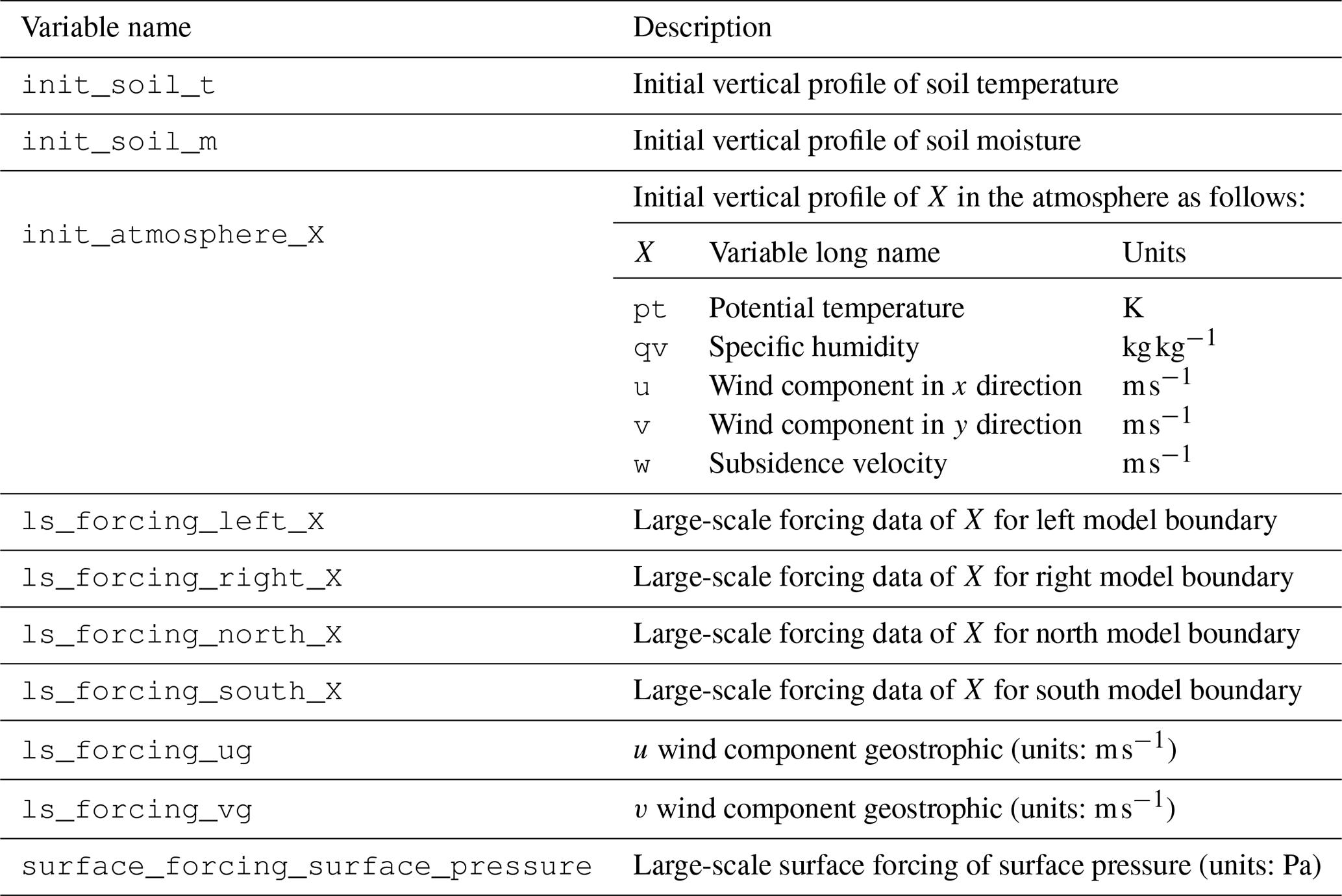
Following the PALM Input Data Standard (PIDS) (https://palm.muk.uni-hannover.de/trac/wiki/doc/app/iofiles/pids, last access: 23 April 2021), the dynamic driver must include initial vertical profiles of the atmosphere and soil, the lateral and top boundary conditions of the atmosphere, and the time series of the surface pressure (Table 1). Note that the variables listed in Table 1 are based on PIDS v1.9. While some variable names may be changed in future updates of PALM, these can be modified in the WRF4PALM code in such cases.
3.1 WRF4PALM framework
The new WRF4PALM (available on https://github.com/dongqi-DQ/WRF4PALM, last access: 23 April 2021) is based on WRF2PALM initially developed by Faria (2019). Modifications and changes made to WRF2PALM to create WRF4PALM are described in Appendix A.
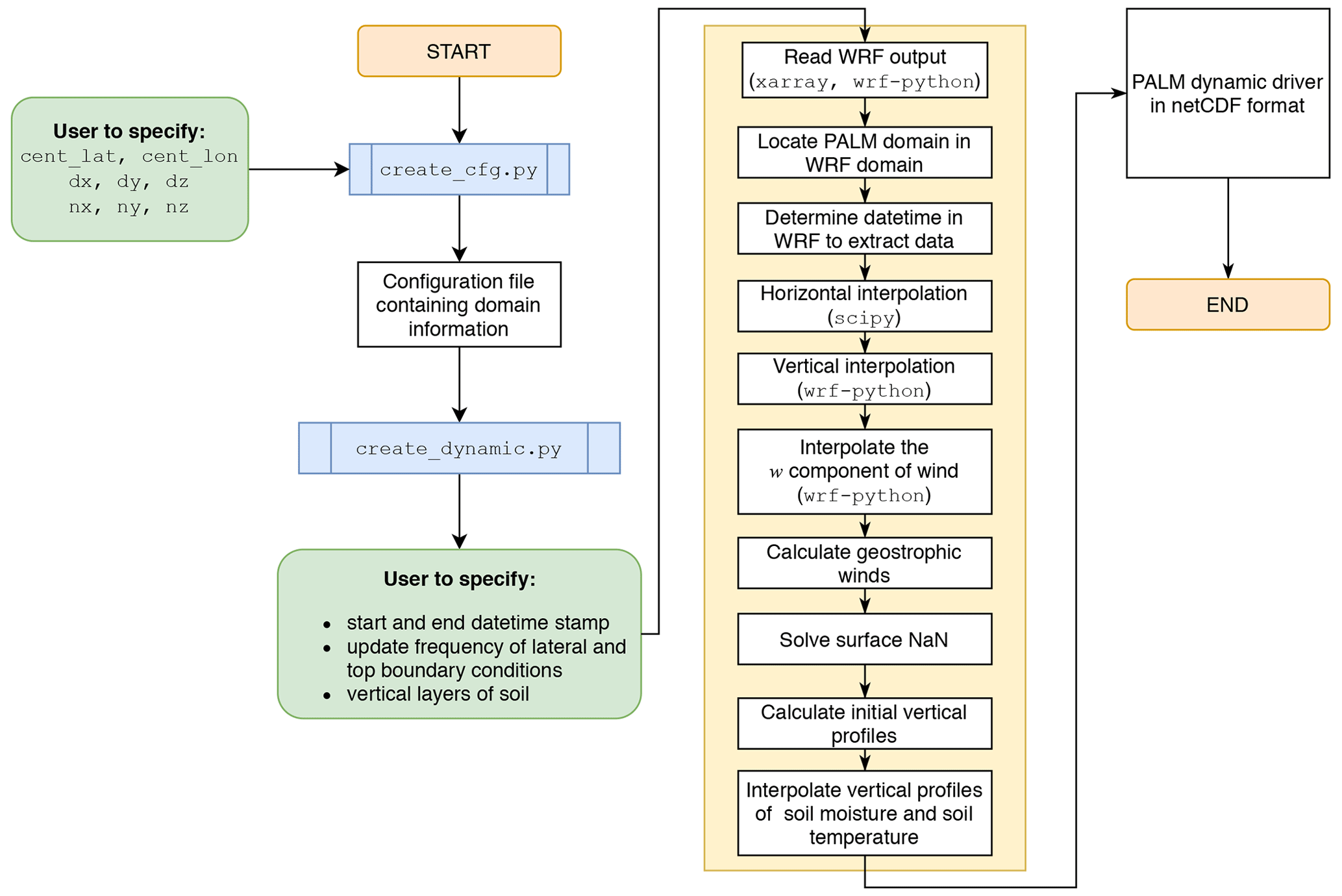
Figure 1The code structure of WRF4PALM. Green boxes indicate input from users. Blue boxes indicate the Python script used. The big yellow box illustrates the processes used to interpolate and pass WRF dynamical fields to the PALM dynamic driver. White boxes outside the yellow box indicate output files of WRF4PALM.
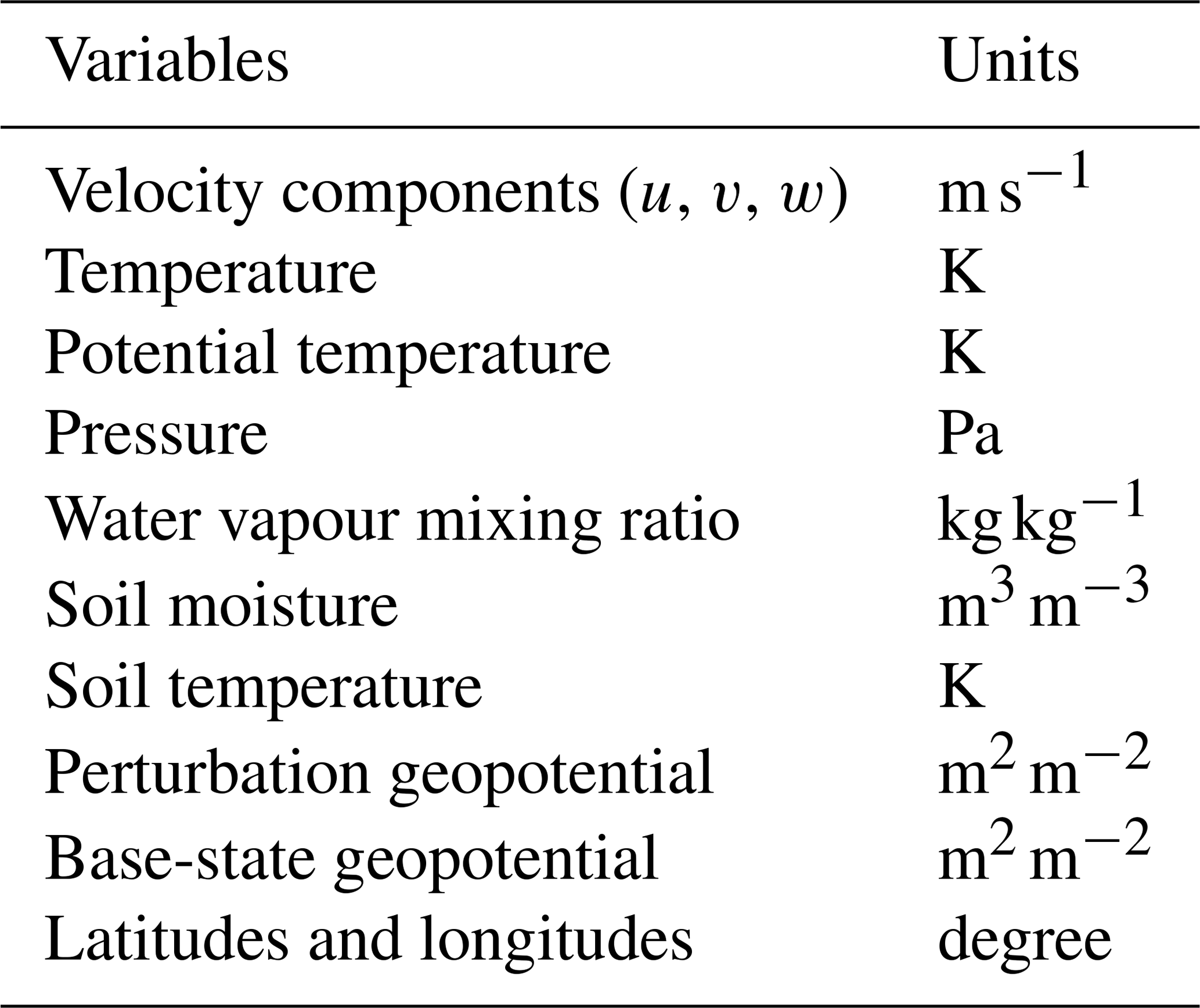
The data passed from WRF to PALM include velocity fields, thermodynamic components (pressure, temperature, potential temperature, and water vapour mixing ratio), soil features, vertical grid structure (geopotential), and geographical information (Table 2). The code structure of WRF4PALM is shown in Fig. 1. WRF4PALM is written in the Python3 programming language. Two major Python scripts comprise WRF4PALM. One is create_cfg.py, which reads user input and specifies the PALM domain within the WRF domain using latitude and longitude bounds. The other is create_dynamic.py, which processes WRF dynamical fields to create the PALM dynamic driver. Detailed step-by-step instructions for running WRF4PALM are given in Appendix B.
The PALM grid configuration prescribes how the WRF output needs to be interpolated onto the PALM grid cells along west–east (nx), south–north (ny), and bottom–top (nz) coordinates and the corresponding grid spacing along each direction (dx, dy, and dz respectively). The latitude and longitude of the centre of the PALM domain must be provided to specify the PALM domain location in the WRF domain. By obtaining the aforementioned domain configuration information from users, the create_cfg.py script then generates a configuration file containing latitudes and longitudes for the north, south, east, and west lateral boundaries and a grid configuration for the PALM domain. The configuration file then acts as an input for create_dynamic.py to finish the interpolation. WRF4PALM also allows users to apply stretched grid spacing along the z direction. Identical to parameters used in the PALM input parameter list, users must define dz_stretch_level, dz_stretch_factor, and dz_max for vertically stretched grid spacing.
The create_dynamic.py script requires users to provide their own WRF output. WRF offers an abundance of choices of parameterisations for microphysics, radiation, surface layer, etc. Users also have a high degree of freedom to choose the meteorological data for initialisation, geospatial data, and projection of the simulation domain. Although optimal WRF configurations will depend on the user's own research interests, any WRF output containing data described in Table 2 is considered applicable for WRF4PALM.
PALM also requires the start and end time stamps (in YYYY, MM, DD, HH format) and lateral and top boundary conditions update frequency to be provided by users. The lateral and top boundary conditions can update from every 1 min to every 6 h (or more) depending on the temporal frequency of WRF output and the user's own research needs. The thickness of the individual soil layers (dz_soil) to be used in PALM must be specified in create_dynamic.py. The default eight-layer configuration of WRF4PALM is the same as that described in Maronga et al. (2015).
Because both PALM and WRF use the Arakawa Cartesian grid staggering (staggered Arakawa C-grid; Harlow and Welch, 1965; Arakawa and Lamb, 1977), no transformation is required in PALM for staggered data. After reading the input parameters described above, the script first extracts WRF data for the specified period and location required for PALM. Potential temperature, air temperature, and pressure fields are read using the getvar function embedded in the WRF-Python package (Ladwig, 2019). Other variables, such as water vapour mixing ratio and wind field, are read using the xarray package (Hoyer and Hamman, 2017). Other than the vertical component of wind (w), all WRF variables are first interpolated on each horizontal field from the WRF domain onto the PALM horizontal Cartesian grid. The horizontal interpolation uses the SciPy package (Virtanen et al., 2020). The WRF data that were horizontally interpolated to the PALM grid are then vertically interpolated onto the PALM vertical Cartesian physical height levels. This requires the interplevel function in the WRF-Python package (Ladwig, 2019), which reads the WRF physical height levels and interpolates the given data onto required PALM vertical levels as defined in the PALM domain configuration file created by create_cfg.py. The WRF physical height levels are calculated using
where PH is the perturbation geopotential in m2 s−2, PHB is the base-state geopotential, and g is gravitational acceleration (9.81 m2 s−2). Equation (1) only gives staggered vertical height levels, which are then destaggered using the destagger function in the WRF-Python package (Ladwig, 2019) for vertical interpolation of variables that are not vertically staggered. When WRF is operated under RANS mode, the value of the vertical component of wind (w) does not represent any turbulence and could be very small in WRF. These small values may lead to possible missing values in the horizontal and subsequently the vertical interpolation. In order to avoid this issue, the vertical component of wind (w) from WRF is first interpolated vertically to PALM vertical-staggered Cartesian physical height levels using staggered vertical height levels calculated by Eq. (1) and interplevel function in the WRF-Python package (Ladwig, 2019). Then, the vertically interpolated data are interpolated horizontally to the PALM horizontal Cartesian grid. Once all the interpolation processes of the aforementioned variables are completed, geostrophic winds are calculated assuming geostrophic balance:
where ρ is air density in kg m−3, f is the Coriolis parameter, P is pressure, and x and y are coordinates along west–east and south–north respectively. Note that as commented in the PALM 6.0 Overview (Maronga et al., 2020) and in the PALM mesoscale nesting interface description (Kadasch et al., 2020), geostrophic winds are not required in the dynamic driver at present. Users can exclude the geostrophic wind forcing by amending the WRF4PALM code themselves.
The height levels in WRF are terrain following (Skamarock et al., 2019) while the Cartesian topography in PALM allows for explicitly resolving obstacles such as buildings and orography (Maronga et al., 2015). Due to such differences in topography representation, the vertical interpolation can lead to Not a Number (NaN) values near the ground surface when WRF data are vertically interpolated onto PALM vertical levels below the first WRF model level. It would be inefficient to create NaN masks and filter data to fit the entire topography and all surface geometries in PALM simulations. Hence, the surface NaN solver is applied to fill the NaN values near the surface. For all the scalar variables and the vertical velocity (w), the surface NaN values are filled by taking the values from the lowest level where valid values exist at the grid point. For horizontal components of velocity (u and v), a logarithmic fit is applied. After solving surface NaN values, the initial vertical profiles are calculated by taking the horizontal average of velocity components, potential temperature, and water vapour mixing ratio at the initial time for each vertical level. The time series of surface pressure in the dynamic driver is the time series of horizontal average of pressure at the lowest level after interpolation. Soil moisture and temperature are interpolated to soil layers provided by users. Due to the difference in the grid resolution and data sources between WRF and PALM, all the soil moisture for water bodies in WRF (where soil moisture is equal to 100 %) is replaced by the median value of land soil moisture in the given PALM simulation domain to avoid mismatch between the PALM and WRF landmasks. To take into account water bodies in PALM, a netCDF static driver input file is required (Heldens et al., 2020), where the types and locations of water bodies are specified. Details about static files used in this work are presented in Sect. 3.2. WRF4PALM also gives the soil information at each soil layer (soil_moisture, soil_temperature, and deep_soil_temperature, identical to PALM input parameters), which can be added into the input parameter list of the PALM land surface model. Details of algorithms applied in WRF4PALM are provided in the online documentation of WRF4PALM.
The dynamic driver of PALM generated by the create_dynamic.py script only contains meteorological and sub-surface fields from WRF and does not encompass any parameterised processes. Since turbulence is completely parameterised in WRF, it is also not included in the dynamic driver. In order to obtain realistic flow characteristics, non-cyclic boundary conditions must be applied. When non-cyclic boundary conditions are used with offline nesting, because no turbulence is included in the inflow, either a large domain is required to allow sufficient space and time for turbulence to develop or the synthetic turbulence generator (STG) must be applied (Gronemeier et al., 2015).
3.2 PALM static driver
To resolve and realise near-surface microscale structures, PALM can read a netCDF static driver file (hereafter static driver) as an input. The static driver includes information on buildings, streets, vegetation, soil, water bodies, etc., in the model domain (Heldens et al., 2020). Due to high variability in geospatial data availability and quality across the world, there is no standard process to generate the PALM static driver. WRF4PALM does not require users to provide a static driver, which is applicable to both realistic simulations (with a static driver) and relatively idealised simulations (without a static driver). However, we recommend that users include the static driver in PALM simulations for more realistic and representative results to understand the impact of microscale surface structures. In the case studies described later, a static driver is included. We adopted a similar procedure described in Heldens et al. (2020) to create the static driver. Various geospatial data sources are used including
-
digital surface model (DSM) and digital elevation model (DEM) from Envirionment Canterbury Regional Council (2020)
-
street and pavement type information from OpenStreetMap (https://planet.openstreetmap.org/, last access: 18 May 2020)
-
building information from New Zealand building outlines dataset (Land Information New Zealand, 2020a)
-
land cover classification data from the Land Cover Database (LCDB) version 5.0, Mainland New Zealand (Landcare Research, 2020)
-
water bodies information from New Zealand parcels dataset (Land Information New Zealand, 2020b).
Two case studies are presented here to demonstrate the performance, stability, and applicability of WRF4PALM. The local solar time, i.e. New Zealand daylight time (NZDT), is used for both case studies presented below. Both the case studies were centred on Christchurch airport, New Zealand (43.4864∘ S, 172.5369∘ E). Christchurch sits in the Canterbury Plains and in the zone of mid-latitude westerlies in the Southern Hemisphere. A succession of subtropical anticyclones and depressions progress eastwards over the city (Macara, 2016). Westerly flows over Christchurch usually bring high clouds and sunshine while easterly flows sometimes lead to cloudiness and rainfall in Christchurch. The two case studies shown illustrate two simulation scenarios from real weather events that occurred in Christchurch, representing synoptic forcing from north-westerly airflow and from easterly and north-easterly flow modulated by a diurnal forcing. In this study, ground-based measurements are obtained from an automatic weather station (AWS) operated by the New Zealand Meteorological Service (MetService) at Christchurch Airport.
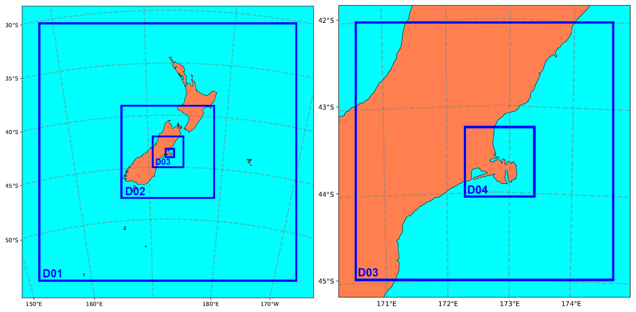
Figure 2WRF domains configuration. Domains D01, D02, D03, and D04 with grid spacing of 27, 9, 3, and 1 km respectively (contains imagery © Cartopy).
4.1 Model configuration
The Advanced Research WRF (ARW) system version 4.0 (Skamarock et al., 2019), WRF4PALM, and PALM model system 6.0 (revision 4550) (Maronga et al., 2015, 2020) are used for the case studies. Figure 2 shows the WRF domain configuration with four domains having horizontal grid spacings of 27, 9, 3, and 1 km respectively. WRF is initialised with ERA5 data, the fifth generation of European Centre for Medium-Range Weather Forecasts (ECMWF) atmospheric reanalysis of the global climate (Hersbach et al., 2019). The WRF simulation uses the contiguous US (CONUS) physics suite (Liu et al., 2017). This physics suite includes the microphysics parameterisation developed by Thompson et al. (2008), the Tiedtke cumulus parameterisation (Tiedtke, 1989; Zhang et al., 2011) (domains D01 and D02 only; see Fig. 2; no cumulus parameterisation scheme is applied for domains D03 and D04; see Fig. 2), the RRTMG models (Iacono et al., 2008) for longwave and shortwave radiation, the quasi-normal scale elimination (QNSE) planetary boundary layer (PBL) physics parameterisation (Sukoriansky et al., 2005), the eta similarity scheme (Monin and Obukhov, 1954; Janjić, 1994, 1996, 2001) for surface layer parameterisation, and the unified Noah land surface model (Tewari et al., 2016). Both WRF simulations presented in this study have a spin-up time of at least 24 h and do not have data assimilation technique applied.
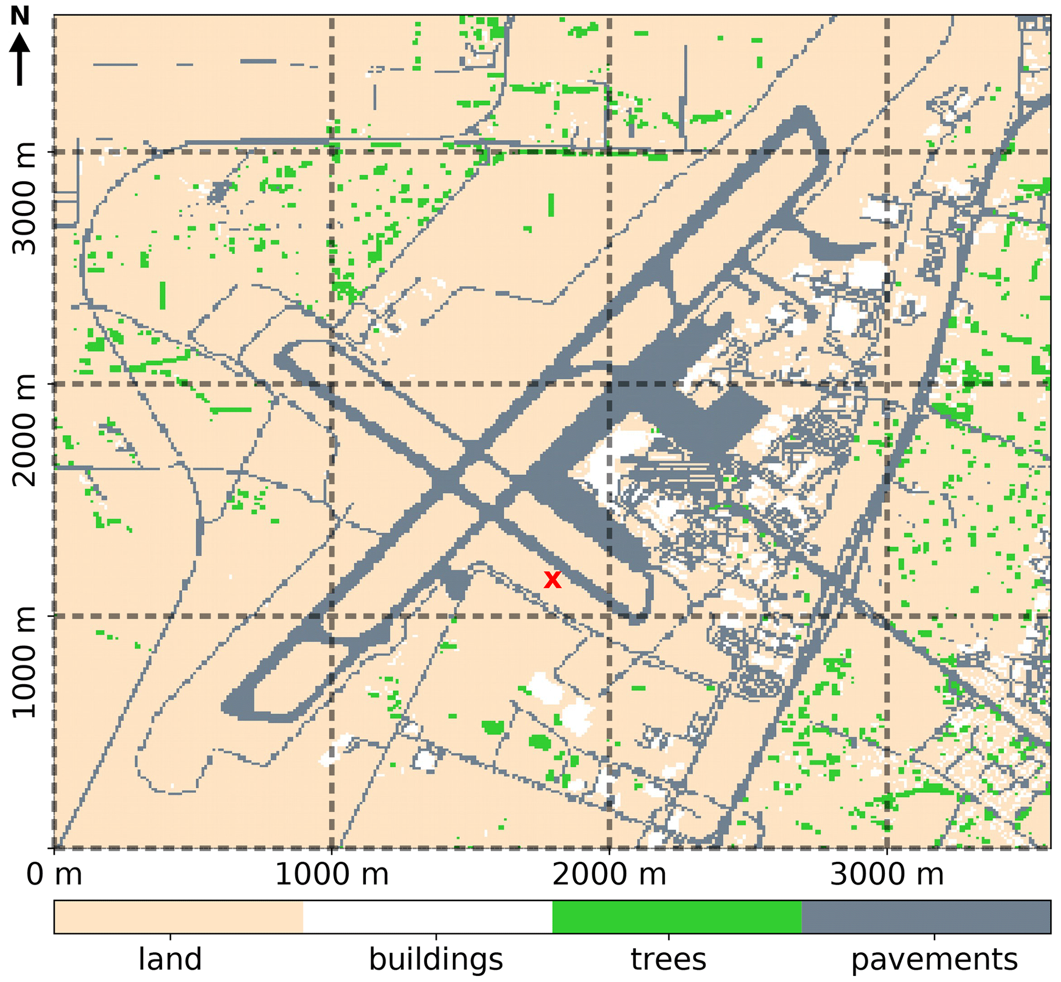
Figure 3PALM modelling domain (3.6 km × 3.6 km) for the north-westerly case. Dotted black lines illustrate the grid size of the WRF model. Buildings are in white, trees are in green, pavements are in grey, and other types of surface are coloured in sand yellow. The red cross shows the AWS location.
Both of the PALM simulations described in the case studies use the following sub-models embedded in PALM: radiation model, land surface model, urban surface model, plant canopy model, synthetic turbulence generator, and offline nesting module. Since this work only aims to demonstrate WRF4PALM's applicability and give an overview of WRF4PALM's performance, the 1 km grid spacing WRF output is directly processed to 10 m grid spacing PALM. The time-dependent 10 m grid spacing boundary conditions are stored in the dynamic driver processed by WRF4PALM. Both of the simulations use non-cyclic boundary conditions to represent realistic meteorological conditions. STG is used in this study to reduce the adjustment zone size near the boundary and to accelerate turbulence development. STG imposes perturbations on the boundary conditions given by the dynamic driver. STG embedded in PALM adopted the technique described by Xie and Castro (2008), which is described in detail in Kadasch et al. (2020). When PALM reads synoptic conditions from the dynamic driver and generates turbulence with STG, a small flow adjustment zone near lateral boundaries may still appear in the simulation. Hence, although the domain configurations of the two case studies are identical (for details, see Table 3), the domain locations are different in order to avoid possible boundary artefacts introduced by STG when comparing model data with observational data at the AWS site. In both PALM simulations, the lateral and top boundary conditions interpolated from WRF are updated hourly. Rayleigh damping at a factor of 0.01 is used near the top boundary (2900 m) to prevent reflection of gravity waves. The STG is called every second with an adjustment interval of 30 s.
Table 3PALM domain configuration for the case studies.
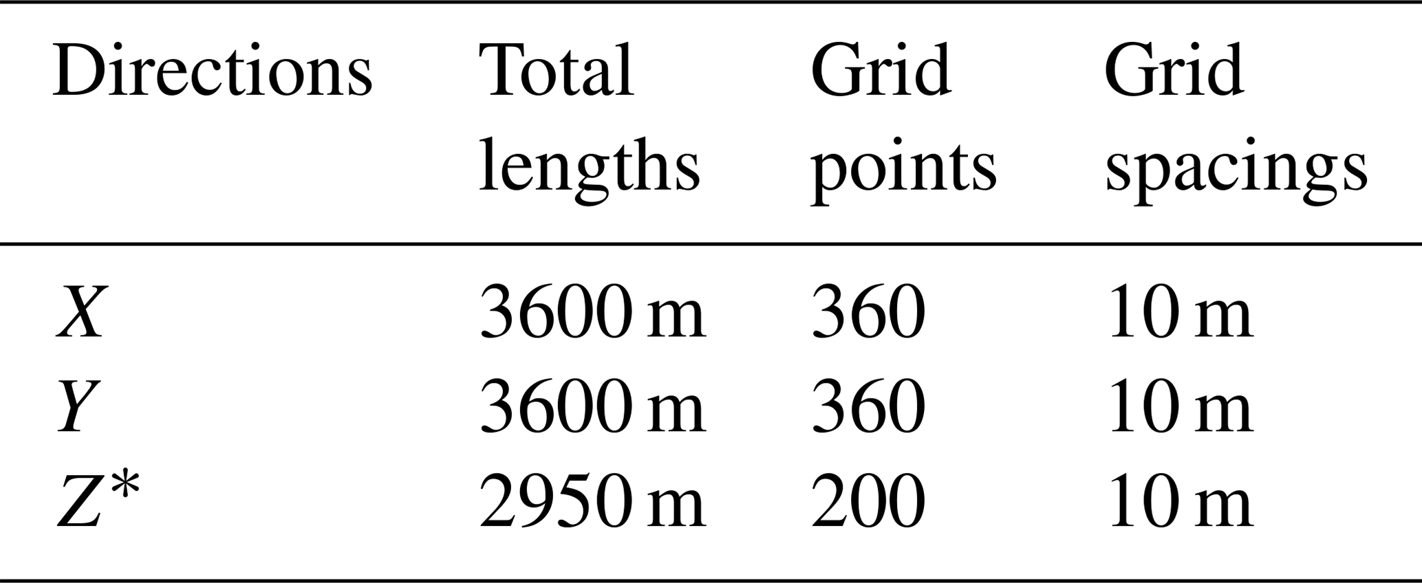
∗ Vertical grid spacing is trenched with a factor of 1.02 above z=1200 m with max vertical grid spacing of 30 m.
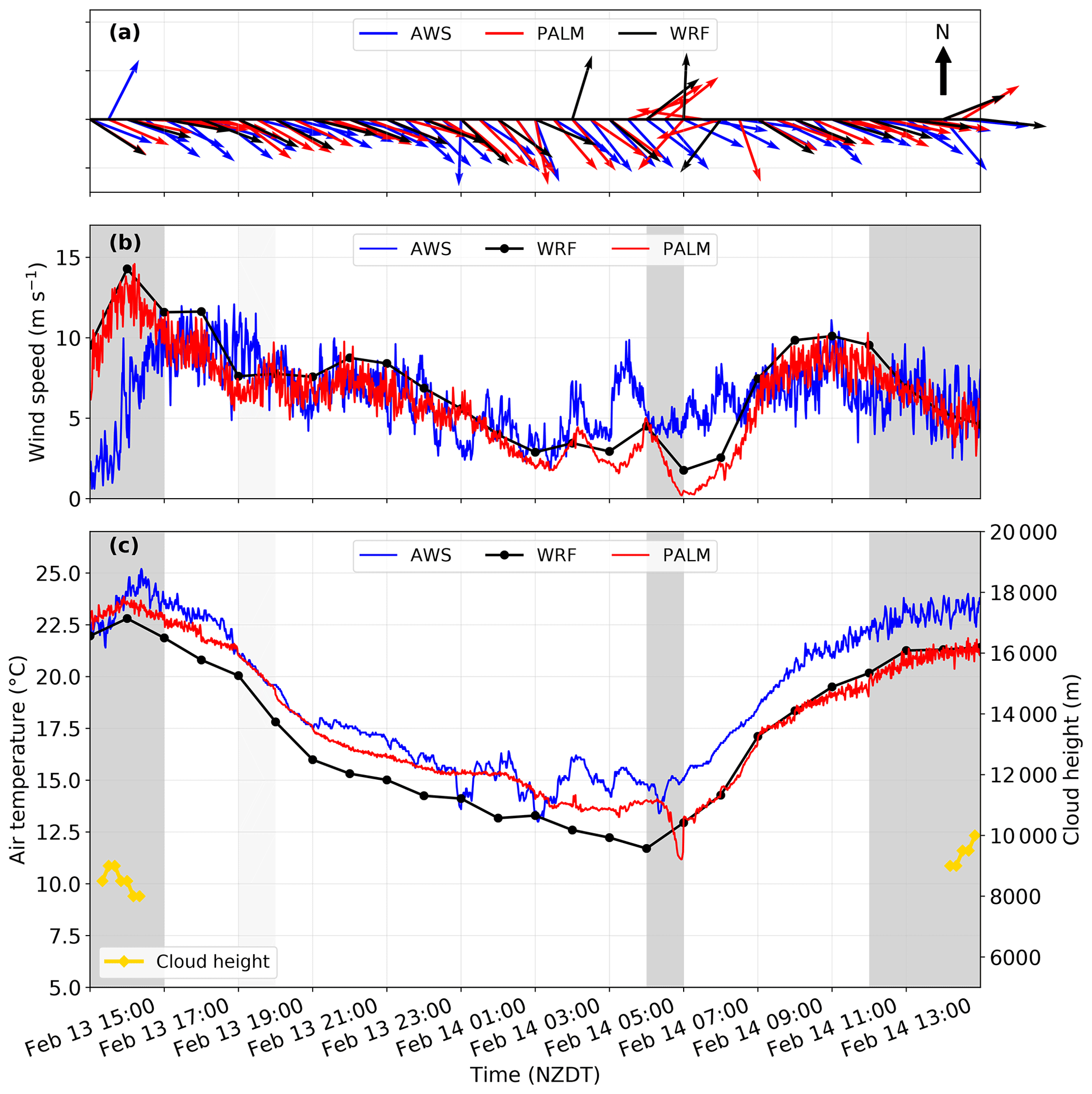
Figure 4The time series of simulated (a) wind direction, (b) wind speed, and (c) air temperature for the north-westerly case between 15:00 NZDT, 13 February and 15:00 NZDT, 14 February 2017 compared with observations (labelled as AWS). In panel (c) the yellow line indicates cloud height observed at the AWS. In panels (b) and (c), the shaded grey periods indicate when clouds are simulated in the WRF model. Only 30 min PALM and observational data for wind direction are shown in (a) to avoid overlapping of arrows.
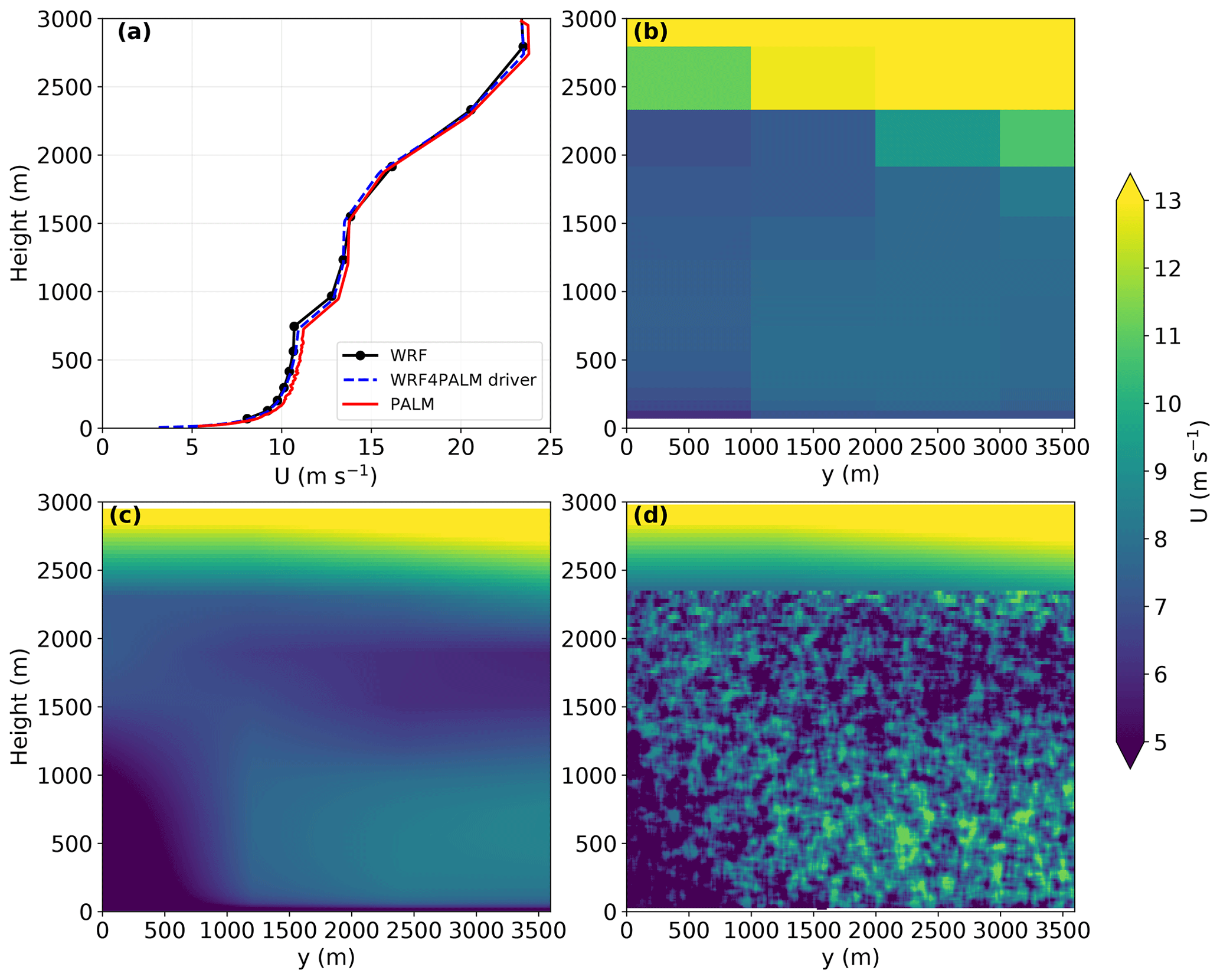
Figure 5(a) Vertical profiles of the u component of winds in WRF, the WRF4PALM dynamic driver, and PALM at the initial time. The profiles taken from WRF and PALM are both horizontally averaged. Vertical cross sections of the u component of winds taken from WRF (nearest four grid cells) (b), the dynamic driver (c), and PALM (d) at 14:00 NZDT, 14 February 2017.
4.2 North-westerly case
During the late afternoon of 13 February 2017, the AWS operated by NZ MetService situated at the Christchurch airport measured strong north-westerly flows. The PALM simulation domain and the AWS location are shown in Fig. 3. The 3.6 km (east–west) × 3.6 km (south–north) simulation domain is designed to: (1) include the AWS in order to compare the model data with the observational data and (2) avoid possible artefacts produced by STG near the north and west lateral boundaries. A narrow zone of laminar flows near the lateral boundaries at inflow can appear in the simulation due to the flow adjustment zone created by STG. As shown in Fig. 4, this PALM simulation includes the 24 h period between 15:00 NZDT, 13 February and 15:00 NZDT, 14 February 2017, which have seen the sustained north-westerlies over Christchurch. In Fig. 4, the time series of the WRF modelling data have an hourly temporal interval while both PALM modelling data and observational data are 1 min averages. Here both PALM and WRF winds are at 10 m in order to compare with 10 m winds measured by the AWS. Both PALM and WRF modelled temperature data shown in Fig. 4 are 2 m data to represent surface air temperatures. In order to show wind direction clearly and avoid overlapping data, only 30 min wind direction PALM and observational data are shown in Fig. 4. The time series of wind direction, wind speed, and air temperature show good agreement between the observational data and the modelled data. WRF overestimated wind speed during the first 2 h shown in Fig. 4 and underestimated wind speed between 05:00 and 08:00 NZDT, 14 February. In addition, the air temperatures simulated by WRF are approximately 2 ∘C lower than the observed temperature during the entire 24 h period. Table 4 compares the modelled surface temperature and wind speed with the observational data. The root mean square error (RMSE),
and index of agreement (IOA),
are used for the comparison between modelled and observational data, where Fi () indicates model estimates or predictions, Oi () indicates the pairwise-matched observations, and is the mean value of observations (for details of the equations see Eq. 2 in Chai and Draxler, 2014 and Eq. 3 in Willmott et al., 2012 respectively). Both RMSE and IOA are measures of the degree of model prediction error. The smaller the RMSE, the better the model fits to the observations. In terms of IOA, a value of 1 indicates a perfect match while 0 indicates no agreement at all. The calculation is applied to the surface time series data shown in Fig. 4. Hourly averages of both PALM-simulated data and the observational data are taken in order to compare them with the WRF-simulated hourly data. Based on RMSE (2.02 for temperature and 2.70 for wind speed) and IOA (0.72 for temperature and 0.50 for wind speed) given in Table 4, WRF results are satisfactory compared with other WRF studies. For example, the best RMSE and IOA for wind speed in Indasi et al. (2017) are 2.30 and 0.66 respectively while they also have simulations with RMSE of 4.21 and IOA of 0.43; temperature simulated by WRF in Bhati and Mohan (2018) has RMSE between 3.87 and 7.99 and IOA between 0.58 and 0.81. Overall, PALM has smaller RMSE and higher IOA than WRF meaning that PALM has better performance than WRF regarding surface temperature and wind speed estimation in this case. The comparison between PALM and WRF also shows good agreement (IOA of 0.87 and 0.75 for surface temperature and wind speed respectively). The improvement in observation-related RMSE and IOA by PALM is due to the inclusion of surface geometries and the LES ability for better resolving near-surface turbulence.
Table 4Comparison of RMSE and IOA between the AWS observational data, the WRF modelling data, and the PALM modelling data at surface. Here, wind indicates wind speed.
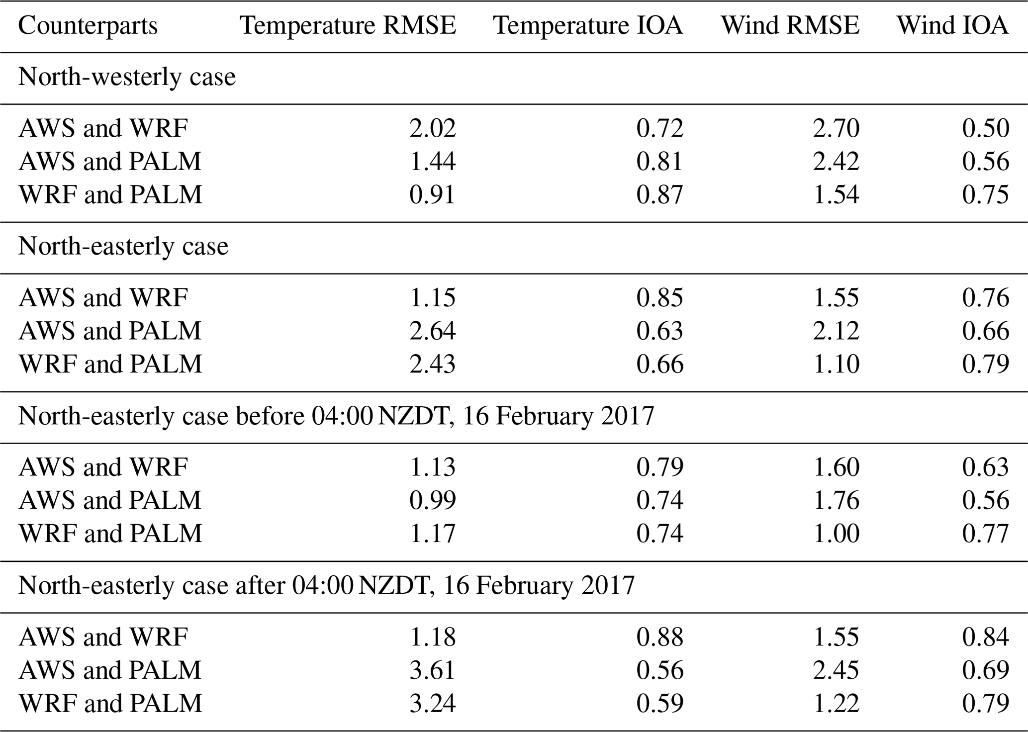

Figure 6The north-westerly case. Vertical profiles of the u component of winds (a–d), v component of winds (e–h), and potential temperature (θ) (i–l) taken from PALM and the WRF model at the times indicated in the figures (from left to right).
Throughout the 24 h period, the results in PALM align with those from WRF. The time series of surface winds and temperatures in PALM shown in Fig. 4 are similar to those in WRF, while PALM shows higher surface temperatures than WRF before 05:00 NZDT, 14 February 2017. To further validate the performance of WRF4PALM, comparisons between WRF, the WRF4PALM dynamic driver, and PALM are carried out. Figure 5 compares the profiles of the u component of winds between WRF, the WRF4PALM dynamic driver, and PALM. The profiles include (1) the initial vertical profiles and (2) left (west) boundary conditions (south–north vertical cross section at the left boundary). Profiles of other parameters in the dynamic drivers are not shown here. The WRF profiles are interpolated by WRF4PALM to the dynamic driver, which is further used as an input for PALM offline nesting. As shown in Fig. 5, profiles in the dynamic driver are generally identical to profiles in WRF meaning that WRF data are successfully interpolated and processed by WRF4PALM. Differences between profiles in PALM and WRF can be spotted (Fig. 5), which are due to the turbulence generated by the STG embedded in PALM. Figure 5 shows that WRF4PALM successfully interpolates dynamics from WRF and passes them to PALM through the dynamic driver. The boundary layer height is automatically calculated in PALM, which is 2300 m in Fig. 5d.

Figure 7The north-westerly case. South–north vertical cross sections of the u component of winds taken from the WRF model (a) and PALM (b) at 14:00 NZDT, 14 February 2017. Horizontal cross sections of the u component of winds taken from the lowest level in the WRF model (c) and 5 m height in PALM (d) at 14:00 NZDT, 14 February 2017. White areas indicate terrain and buildings higher than 5 m above the lowest level in the PALM simulation domain.
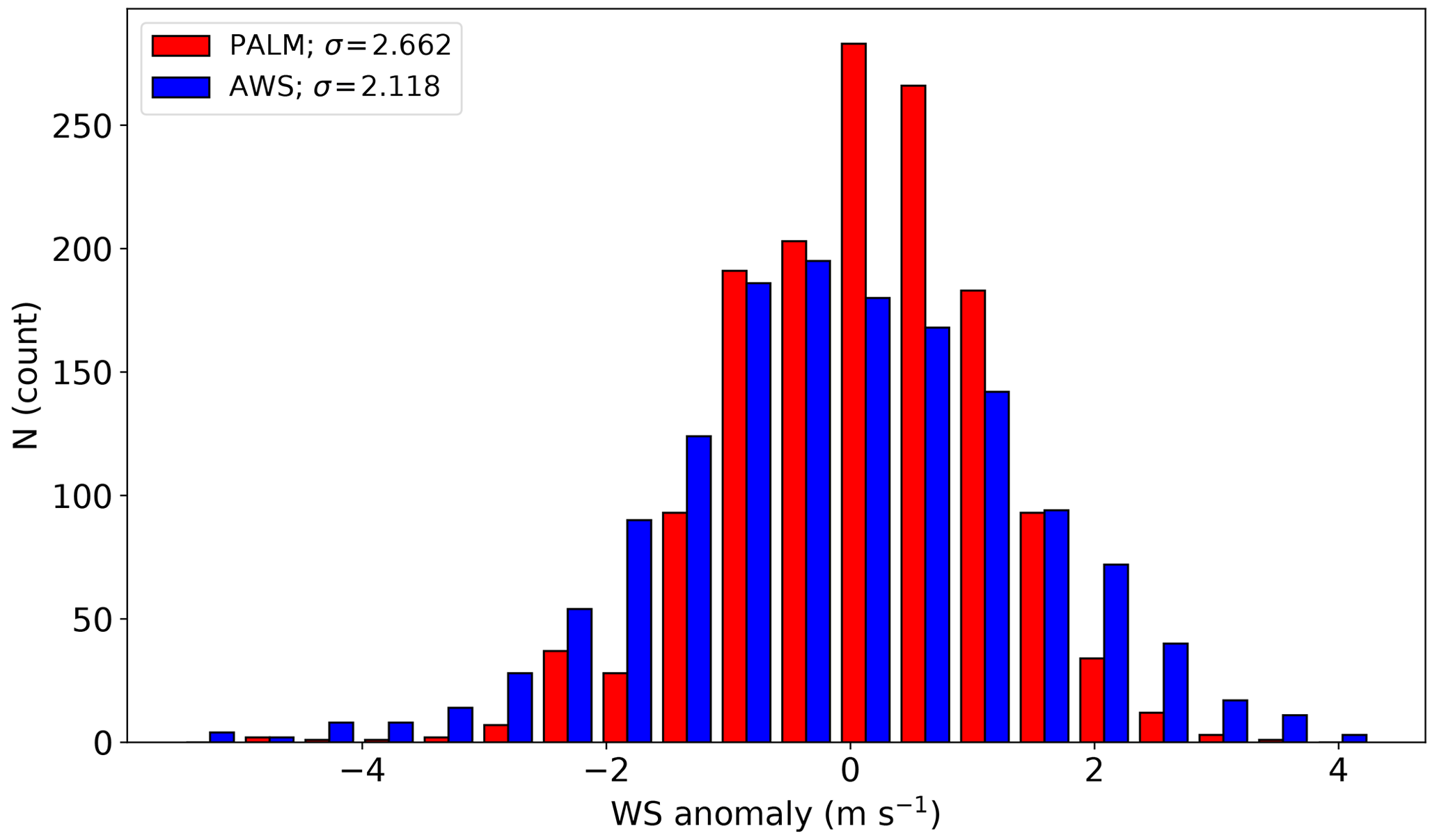
Figure 8Comparison of the range and distributions of hourly wind speed anomalies between PALM and the observational data (labelled as AWS) for the 24 h period of the north-westerly case. σ is the standard deviation of the anomaly data.
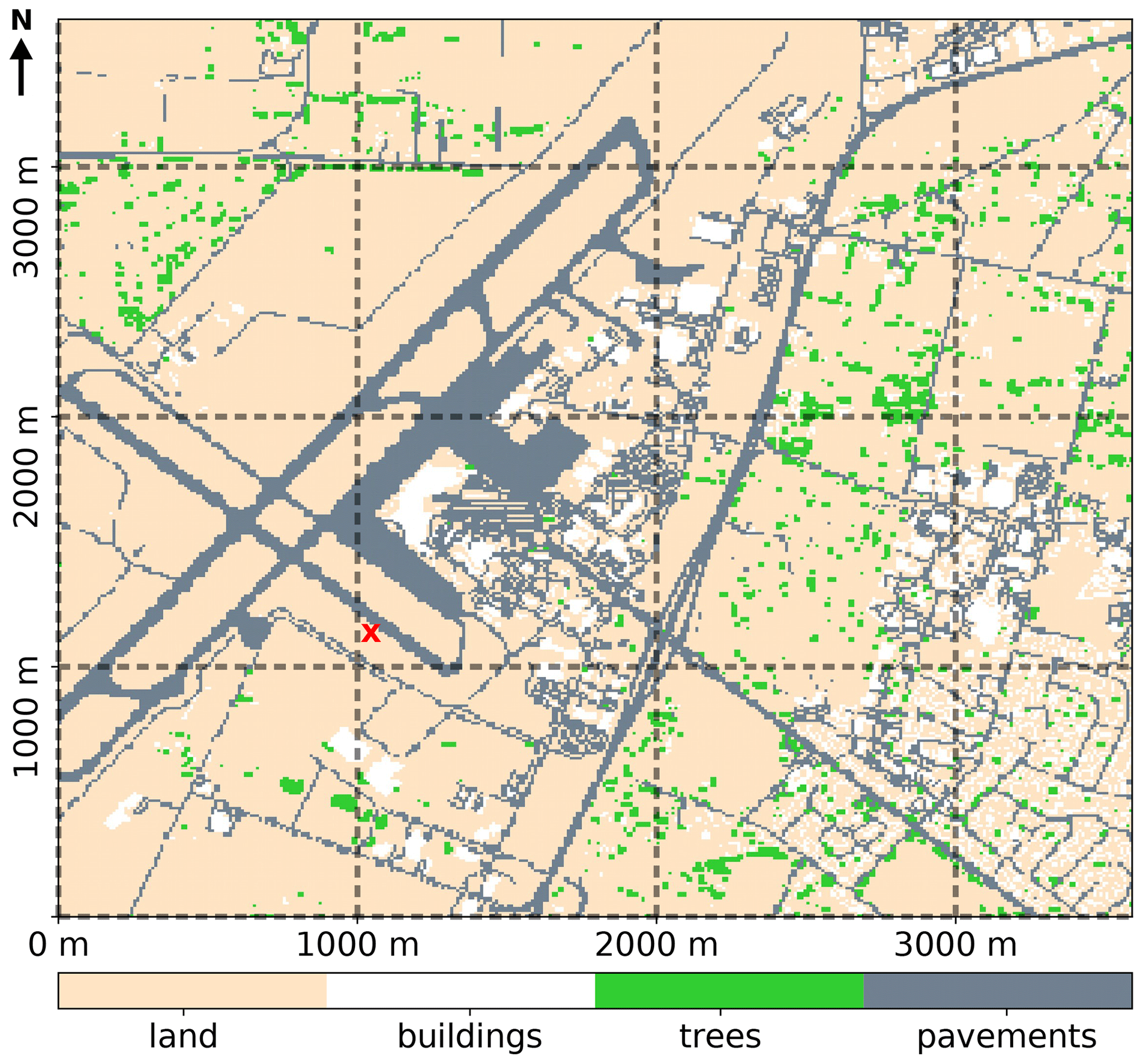
Figure 9As in Fig. 3, but for the north-easterly case.
The vertical profiles of the u component and v component of winds and potential temperature (θ) at 15:00 and 21:00 NZDT on 13 February 2017 and at 03:00 and 09:00 NZDT on 14 February 2017 in PALM are almost identical to vertical profiles in WRF as shown in Fig. 6, and the boundary layer heights in WRF and PALM are consistent over time. The maximum boundary layer height (MBLH) is around 1.5–1.8 km in both WRF and PALM. The only major difference in the vertical profiles between the two models can be spotted near the surface. This difference is due to the impact of surface canopy because PALM is able to explicitly resolve vegetation and building structures in the simulation. A spatial resolution of 10 m may not be sufficient to represent detailed structures of buildings, but such resolution allows PALM to adequately represent most of the surface geometries in the model domain. We believe the high similarity between PALM and WRF demonstrates successful offline nesting using WRF4PALM. The lateral and top boundaries of PALM are offline nested with WRF, and the mesoscale forcings from WRF are updated every hour. Driving an LES model using hourly update cycles from a mesoscale model ensures mesoscale disturbances are represented, but it may also hinder the microscale boundary layer dynamics developing their own unique state (Schalkwijk et al., 2015; Heinze et al., 2017). Hence, PALM follows most of the dynamics processed from WRF and this could be further investigated by relaxing the update cycle of PALM's boundary conditions. In addition to the turbulent time series of PALM shown in Fig. 4, Fig. 7 compares the vertical and horizontal cross sections between WRF and PALM. The WRF cross sections presented in Fig. 7 are the nearest four WRF grid points (4 km × 4 km) processed to the PALM domain (3.6 km × 3.6 km). The cross sections of the two models show that PALM has strong agreement with WRF. However, WRF is not able to resolve any surface geometries because it is a terrain following model and only simulates mesoscale characteristics of airflows. On the contrary, PALM’s Cartesian grid structure allows PALM to resolve all the terrain structure and urban canopy explicitly. White patches and areas shown in Fig. 7d are buildings and terrains that are higher than 5 m above the lowest level in the PALM simulation domain. Microscale characteristics, such as the local lift and drag forces as well as turbulence, are only realised in PALM.
To demonstrate and further validate wind anomalies produced in the PALM simulation, Fig. 8 compares the modelled wind speed anomalies in PALM to the anomalies observed by the AWS. The wind anomalies are calculated by differencing the instantaneous 1 min wind speed from the hourly averaged wind speed for each hour during the 24 h simulation period. As shown in Fig. 8, the modelled anomalies vary from approximately −4.2 to 3.5 m s−1 while the observed anomalies vary from approximately −5.0 to 4.0 m s−1. The standard deviation (σ) of modelled data (2.662) is greater than the observational data (2.118). PALM created more positive anomalies but with lower magnitude. The underestimation in the intensity is likely to result from underpredictions in nighttime turbulence generated by PALM incorporating the STG at inflow or the biases produced in the model due to coarse grid spacing (van Stratum and Stevens, 2015). The spatial resolution used in the PALM simulation is only 10 m, which may not be sufficient to represent the nocturnal boundary layer properly. Despite the underestimation, PALM is able to reproduce the wind trends and directions. The wind anomaly statistics of WRF are not shown here because (1) the RANS mode of WRF only presents average properties of airflows and (2) the WRF output used here only contains hourly data, which cannot give any wind anomaly information at each hour during the simulation period.

Figure 10As in Fig. 4, but for the north-easterly case between 17:00 NZDT, 15 May 2017 and 17:00 NZDT, 16 May 2017.
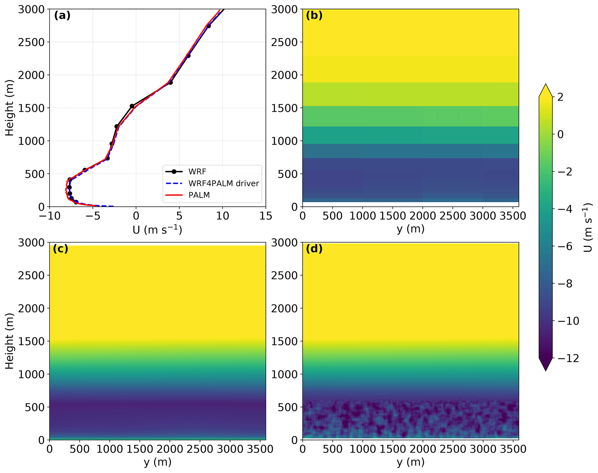
Figure 11As in Fig. 5, but for the north-easterly case. Panels (b), (c), and (d) are at 16:00 NZDT, 16 May 2017.
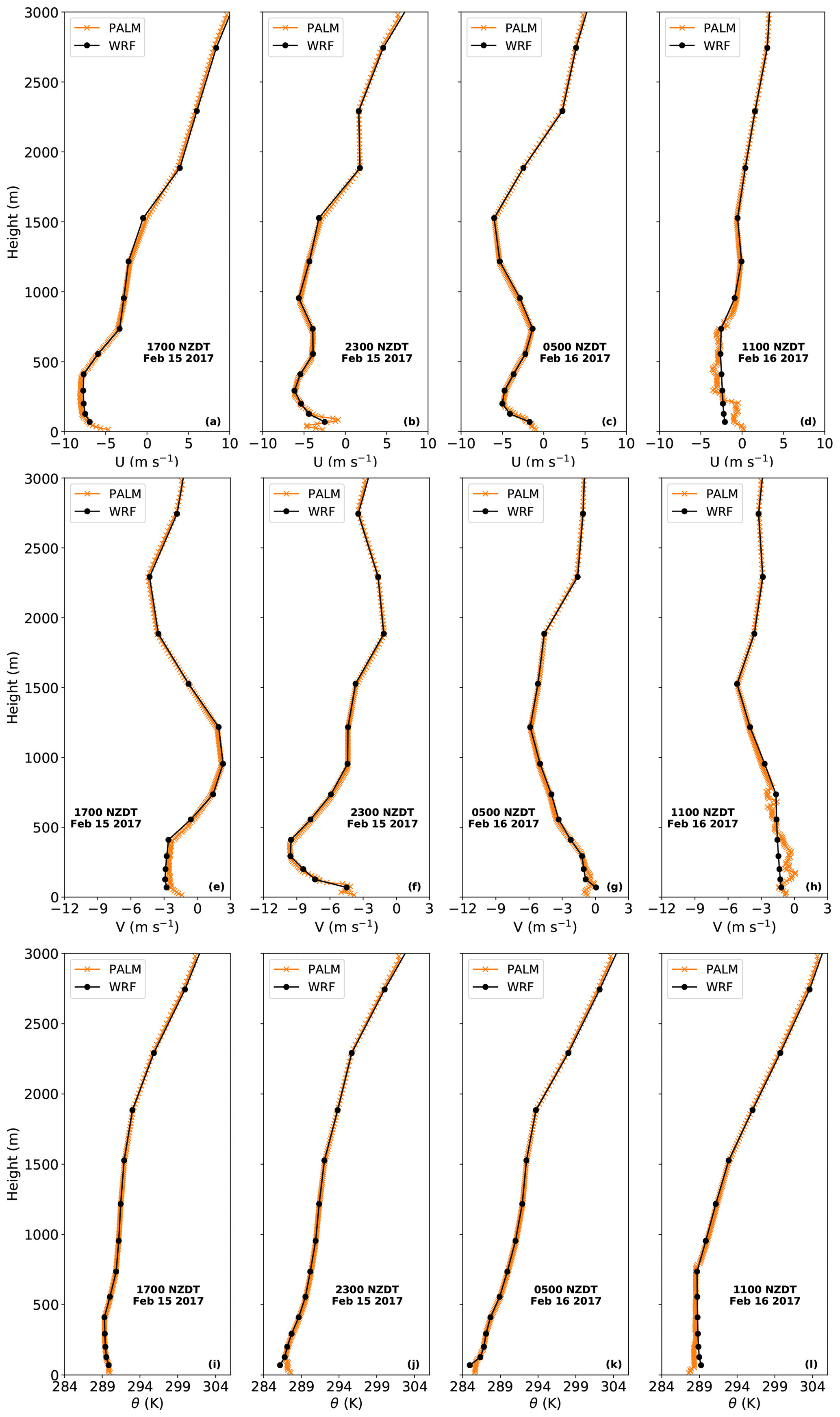
Figure 12As in Fig. 6, but for the north-easterly case between 17:00 NZDT, 15 May 2017 and 17:00 NZDT, 16 May 2017.

4.3 North-easterly case
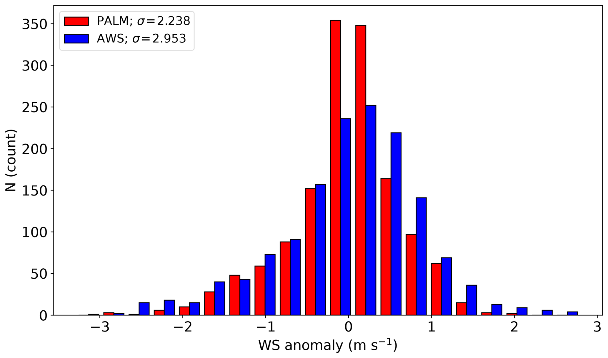
In the late afternoons on 15 February 2017, easterly-north-easterly flows were observed over Christchurch airport. During the early mornings on 16 February 2017, calm northerlies were recorded. Similar to the north-westerly case described in Sect. 4.2, the PALM simulation domain (see Fig. 9) is designed to include the AWS and avoid artefacts near the north and east lateral boundaries. Figure 10 shows the time series of wind direction, wind speed, air temperature, and cloud height during the 24 h PALM simulation period from 17:00 NZDT, 15 February 2017 to 17:00 NZDT, 16 February 2017. Similar to the north-westerly case, profiles in WRF, the WRF4PALM dynamic driver, and PALM are consistent (Fig. 11). The vertical profiles shown in Fig. 12 and the vertical and horizontal cross sections shown in Fig. 13 all show good agreement between PALM and WRF. The MBLH for this case is 900 m in both WRF and PALM. However, PALM does not predict surface temperatures and winds as well as in the north-westerly case described above. For the period after 07:00 NZDT, 16 February (see Fig. 10), PALM follows the increasing trends of surface temperature and wind speed in WRF, but the underestimation of surface temperature in PALM is significant. Wind speed in PALM is approximately 2 m s−1 lower than both the WRF modelled data and the observational data. The largest difference in surface temperature between PALM and both WRF and the observational data is approximately 7 ∘C. In terms of the RMSE and IOA for this case, shown in Table 4, PALM has worse scores than WRF, despite the fact that PALM still has adequate agreement with WRF (IOA of 0.66 and 0.79 for surface temperature and wind speed respectively). The wind anomaly analysis for the hourly averaged wind speed during the entire 24 h simulation period is shown in Fig. 14. In this case, PALM only has an adequate performance in terms of modelling wind anomalies. Similar to the north-westerly case, anomalies simulated by PALM have more positive and smaller values. Due to the bias in the surface wind and temperature, PALM also underestimated wind anomalies significantly. The modelled anomalies vary from approximately −2.8 to 2.0 m s−1, while the observational data show that the anomalies have a range approximately −3.2 to 2.8 m s−1. The standard deviation also shows underestimation in PALM (2.238) compared with the observational data (2.953).
There could be several reasons for the bias in PALM. Regardless of different initialisation situations between the two case studies, cloud cover is suspected to be one particular reason for errors in PALM. In both PALM simulations, the clear-sky radiation scheme is used. This radiation scheme is the simplest scheme in the PALM modelling system and neglects all clouds. The observed cloud height and WRF-modelled clouds are shown in Figs. 4 and 10. Here the variable cloud fraction is used to represent cloud cover in WRF. The grey shaded periods in Figs. 4 and 10 represent when the cloud fraction in WRF is greater than zero. Cloud fractions in WRF were averaged over the closest 10 grid cells over the Christchurch airport. In the north-westerly case, most of the simulation period saw clear skies and only a small number of high clouds (above approximately 7500 m) were observed above the Christchurch airport and WRF generally correctly predicted cloud cover (see Fig. 4). In contrast, the period between 04:00 and 17:00 NZDT, 16 February saw sustained low level clouds (1000 to 3000 m) (see Fig. 10). WRF may have managed to have an adequate estimation of cloud cover during early mornings on 16 February and hence has a better performance than PALM in this north-easterly case. Because no clouds are simulated in clear-sky PALM, the simulated radiation in PALM becomes unrealistic. According to Table 4, the RMSE and IOA of surface temperature in PALM for clear sky periods (before 04:00 NZDT, 16 February) are considerably better than the numbers for cloudy periods (after 04:00 NZDT, 16 February). Another possible reason for PALM's poor performance could be the internal dynamics in PALM. As shown in Fig. 10, PALM simulated a north-westerly airflow near the AWS site near 08:00 NZDT, 16 May 2017. The north-westerly air mass results in a more convective surface and significant decrease in surface temperature in the west part of the PALM simulation domain (not shown). In this north-easterly case, the wind speed during the simulated period is generally low, which cannot offset the convections in PALM domain. We believe the validation results of the PALM simulations with observations are not related to the technique of the offline nesting or WRF4PALM. Rather, the dynamics, weather conditions, or PALM domain configurations may be the possible factors. The PALM domain location in this case is different from the north-easterly case and the sensitivity of the domain grid spacing or domain size may also need to be evaluated. Further studies are required to investigate why PALM underestimates surface temperature and wind speed. However, this is beyond the scope of this study as here we only aim to validate WRF4PALM. Although PALM provides several radiation scheme options and has the bulk cloud module embedded, the detailed dynamics in simulations may vary case by case and hence the optimal simulation setup of PALM must be examined in future simulations.
This study describes a utility WRF4PALM that is developed to generate mesoscale forcing from WRF output for the PALM model system 6.0. Results of the application are also validated by two case studies in Christchurch, New Zealand, in the summer season. WRF4PALM does not require users to pre-process any data manually, but users need to provide their WRF output and PALM domain configuration. WRF4PALM only encompasses mesoscale dynamics from WRF and does not require a static driver of PALM. In order to include surface heterogeneities, the PALM static driver is used in this study when it is necessary to realise microstructures in urban environments and hence to achieve realistic and representative results in PALM simulations. In the case studies, WRF4PALM was applied to two weather events simulated by WRF for a north-westerly case and a north-easterly case in Christchurch, New Zealand. The case studies are designed to demonstrate the numerical stability of WRF4PALM rather than properly validate meteorology in the simulations. As shown in the case studies, overall WRF4PALM is considered to have good stability and is able to process dynamics from WRF to PALM successfully. While PALM inherited most of the characteristics from WRF through the WRF4PALM dynamic driver, PALM's ability to resolve turbulence structure is essential to realise and represent microscale dynamics in urban environments. A comparison of wind anomaly statistics also shows satisfactory agreement between PALM and the AWS observational data.
For future use, the domain size, grid spacing, radiation scheme, and all other model configurations of WRF and PALM need to be evaluated subject to the users' own objectives and scope of research questions. In this study, the lateral and top boundary conditions in the WRF-PALM offline nesting are updated every 1 h meaning PALM is significantly impacted and constrained by WRF. The sensitivity to the relaxation time and the STG configuration to develop initial turbulence need further assessment.
WRF4PALM is distributed as a free and open-source tool. In the future, we aim to optimise WRF4PALM in terms of computation time and to further automate the process. As described in the PALM input data standard, the dynamic driver of PALM can also include boundary conditions of chemistry species, such as PM10, NOx (NO2, NO), and SO4 to simulate air pollution in urban environments. WRF4PALM has the potential to process chemistry data from WRF-Chem (the WRF model coupled with chemistry; Grell et al., 2005) to PALM using a similar interpolation technique as that described in Sect. 3.1. Although several tests and validations have been carried out for WRF4PALM, they may not be conclusive. To improve and extend the use of WRF4PALM, we welcome all users to optimise, modify, and contribute to the code.
Based on ideas and techniques applied in WRF2PALM, the following changes have been made to develop WRF4PALM:
-
add initial vertical profiles interpolated from WRF to initialise PALM
-
modify geostrophic wind calculation
-
add
create_cfg.pyscript to read user input to reduce manual processing -
improve methods for PALM domain configuration, which is almost identical to PALM input parameters
-
interpolation order is modified; horizontal interpolation is performed before vertical interpolation.
-
adjust physical heights calculated from WRF for vertical interpolation.
-
adjust horizontal interpolation method for boundary conditions.
-
adjust PALM domain height calculation for vertical interpolation and calculation of top boundary conditions
-
add staggered coordinates for wind field (u,v, and w) interpolation
-
add 3-D soil moisture and soil temperature profiles interpolated from WRF
-
allow PALM domain size smaller than one WRF grid cell size
-
allow users choose simulation period and update frequency based on WRF model outputs
-
add functions to create coordinate information for PALM self-nested domains
-
add surface NaN solver
-
add parameters and functions to enable vertically stretched grid spacing in the dynamic driver and subsequently PALM.
RAM (random access memory) usage is modified after the aforementioned development and several other small tweaks are made in WRF4PALM. WRF2PALM functions are either removed or modified in WRF4PALM. The following Python functions used in WRF4PALM are based on WRF2PALM:
-
Function to determine the nearest gird cells in WRF to be interpolated to the PALM Cartesian grid:
def nearest(array, number): ''' find nearest index value and index in array. nearest(array, number) return(nearest_number, nearest_index) ''' import numpy as np nearest_index = np.where(np.abs(array-number) == np.nanmin(np.abs(array-number))) nearest_index = int(nearest_index[0]) nearest_number = array[nearest_index] return(nearest_number, nearest_index) -
Function to interpolate WRF data horizontally:
def interp_array_2d(data, out_x, out_y, method): ''' 2d matrix data, x number of points out_x, y number of points out_y, method 'linear' or 'nearest' ''' y = np.arange(0, data.shape[0], 1) x = np.arange(0, data.shape[1], 1) interpolating_function = RegularGridInterpolator((y, x), data, method = method) yy, xx = np.meshgrid(np.linspace(x[0], x[-1], out_x), np.linspace(y[0], y[-1], out_y)) data_res = interpolating_function((xx, yy)) return (data_res) -
Function to interpolate a 1-d array while calculating geostrophic winds:
    def interp_array_1d(data, out_x) :
        '''
        1d matrix data, x number of points out_x.
        Output a linear interpolated array
        '''
        x = np.arange(0, data.shape[0], 1)
        xvals = np.linspace(0, data.shape[0], out_x)
        data_res = np.interp(xvals, x, data)
    return (data_res)
A more detailed manual is available at https://github.com/dongqi-DQ/WRF4PALM (last access: 23 April 2021).
B1 Step 1: specify the domain
Users first need to give the domain information in the create_cfg.py script. The information includes
    case_name_d01 = 'chch_10m_NW' # case name as you prefer, but should be
                                  # consistent with the one used in dynamic script
    centlat_d01   = -43.487       # latitude of domain centre
    centlon_d01   = 172.537       # longitude of domain centre
    dx_d01        = 10            # resolution in meters along x-axis
    dy_d01        = 10            # resolution in meters along y-axis
    dz_d01        = 10            # resolution in meters along z-axis
    nx_d01        = 360           # number of grid points along x-axis
    ny_d01        = 360           # number of grid points along y-axis
    nz_d01        = 120           # number of grid points along z-axis
Run create_cfg.py to create a configuration file containing the domain information for create_dynamic.py.
B2 Step 2: process WRF for PALM
-
Specify case name, which should be the same as the one specified in Step 1.
case_name = 'chch_10m_NW' # case name as specified in create_cfg.py
-
Specify the WRF output file to process.
wrf_file = 'wrfout_domain_yyyy-mm-dd'
-
Specify the start and end time stamp as well as the update frequency of boundary conditions.
dt_start = datetime(2017, 2, 11, 0,) # start time in YYYY/MM/DD/HH format dt_end = datetime(2017, 2, 12, 0,) # end time in YYYY/MM/DD/HH format interval = 2 # specify update frequency -
Specify the depth of soil layers.
dz_soil = np.array([0.01, 0.02, 0.04, 0.06, 0.14, 0.26, 0.54, 1.86]) # this is the default 8-layer setup in PALM -
If stretched vertical grid spacing is desired, specify the following parameters:
dz_stretch_factor = 1.02 # stretch factor for a vertically stretched grid # set to 1 if no stretching is desired dz_stretch_level = 1200 # Height level above which the grid cells # are to be stretched vertically (in m) dz_max = 30 # allowed maximum vertical grid spacing (in m) -
Run
create_dynamic.pyand if successfully executed, a dynamic driver file will be ready.
The WRF model system V4.0 and the WRF Pre-processing System (WPS) V4.0 used in this study are free and open-source numerical atmospheric modelling systems (registration and download are available at https://www2.mmm.ucar.edu/wrf/users/download/get_source.html, last access: 23 April 2021). The PALM model system 6.0 used in this study is freely available online (http://palm-model.org, last access: 23 April 2021) under the GNU General Public License v3. The exact PALM model source code (revision 4550) is available at https://doi.org/10.5281/zenodo.4713316 (Lin, 2020a) or https://palm.muk.uni-hannover.de/trac/browser?rev=4550 (last access: 23 April 2021). WRF4PALM code is freely available at https://doi.org/10.5281/zenodo.4017005 (Lin, 2020b) or https://github.com/dongqi-DQ/WRF4PALM (last access: 23 April 2021) distributed under GNU General Public License v3.0. Details of Python packages used in WRF4PALM are given on the GitHub repository.
All PALM input files for the north-westerly case described in Sect. 4.2, including the static driver, the WRF4PALM dynamic driver, and its configuration file, are available in the Supplement. New Zealand MetService maintains ownership of the raw AWS data and is providing the data to the University of Canterbury on the understanding that it is for the purposes of research. The raw AWS data may not be used for commercial gain. The raw AWS data may not be made available to any third party, unless prior agreement has been obtained from MetService.
The supplement related to this article is available online at: https://doi.org/10.5194/gmd-14-2503-2021-supplement.
RF provided the WRF2PALM code. BK and DL contributed to the initial development of WRF4PALM. DL contributed to major WRF4PALM development and distribution. LB helped DL with setting up WRF simulation. DL carried out the WRF and PALM simulations and analysed the data. MK and LER supervised DL in performing the case studies. DL wrote the manuscript with contributions from BK, MK, and LER. BK, MK, and LER reviewed the manuscript.
The authors declare that they have no conflict of interest.
We would like to thank Iman Soltanzadeh and Neal Osborne from New Zealand MetService for providing automatic weather observations in Christchurch, New Zealand. We thank Rui Caldeira from the Oceanic Observatory of Madeira for internal review of the original manuscript. Dongqi Lin acknowledges Jiawei Zhang at the University of Canterbury for his help regarding technical issues related to PALM simulations. All PALM simulations presented in this study were performed on New Zealand eScience Infrastructure (NeSI) high-performance computing facilities. WRF simulations were performed on the University of Canterbury high-performance computing cluster.
Dongqi Lin and Laura E. Revell received support from the University of Canterbury and the Ministry of Business, Innovation and Employment project Particulate Matter Emissions Maps for Cities (grant no. BSCIF1802). The contribution of Basit Khan was supported by the MOSAIK and MOSAIK-2 projects, which are funded by the German Federal Ministry of Education and Research (BMBF) (grant nos. 01LP1601A and 01LP1911H), within the framework of Research for Sustainable Development (FONA; http://www.fona.de, last access: 10 August 2020). Marwan Katurji was supported by the Royal Society of New Zealand (contract no. RDF-UOC1701). Ricardo Faria was financially supported by the Oceanic Observatory of Madeira Project (grant no. M1420-01-0145-FEDER-000001-Observatório Oceânico da Madeira-OOM).
This paper was edited by Paul Ullrich and reviewed by two anonymous referees.
Arakawa, A. and Lamb, V. R.: Computational design of the basic dynamical processes of the UCLA general circulation model, General circulation models of the atmosphere, 17, 173–265, 1977. a
Baldauf, M., Stephan, K., Klink, S., Schraff, C., Seifert, A., Förstner, J., Reinhardt, T., and Lenz, C.: The new very short range forecast model COSMO-LMK for the convection-resolving scale, WGNE Blue Book, Research activities in atmospheric and oceanic modelling, CAS/JSC Working Group on Numerical Experimentation, Report No. 37, WMO, Geneva, Switzerland, 1–2, 2007. a
Bengtsson, L., Andrae, U., Aspelien, T., Batrak, Y., Calvo, J., de Rooy, W., Gleeson, E., Hansen-Sass, B., Homleid, M., Hortal, M., Ivarsson, K., Lenderink, G., Niemelä, S., Nielsen, K. P., Onvlee, J., Rontu, L., Samuelsson, P., Muñoz, D. S., Subias, A., Tijm, S., Toll, V., Yang, X., and Køltzow, M. Ø.: The HARMONIE–AROME model configuration in the ALADIN–HIRLAM NWP system, Mon. Weather Rev., 145, 1919–1935, https://doi.org/10.1175/MWR-D-16-0417.1, 2017. a
Bergot, T., Escobar, J., and Masson, V.: Effect of small-scale surface heterogeneities and buildings on radiation fog: Large-eddy simulation study at Paris–Charles de Gaulle airport, Q. J. Roy. Meteor. Soc., 141, 285–298, 2015. a
Bhati, S. and Mohan, M.: WRF-urban canopy model evaluation for the assessment of heat island and thermal comfort over an urban airshed in India under varying land use/land cover conditions, Geosci. Lett., 5, 27, https://doi.org/10.1186/s40562-018-0126-7, 2018. a
Chai, T. and Draxler, R. R.: Root mean square error (RMSE) or mean absolute error (MAE)? – Arguments against avoiding RMSE in the literature, Geosci. Model Dev., 7, 1247–1250, https://doi.org/10.5194/gmd-7-1247-2014, 2014. a
Envirionment Canterbury Regional Council: Christchurch and Ashley River, Canterbury, New Zealand 2018, Open Topography, https://doi.org/10.5069/G91J97WQ, 2020. a
Faria, R.: WRF2PALM, available at: https://github.com/ricardo88faria/WRF2PALM (last access: 23 April 2021), 2019. a
Gousseau, P., Blocken, B., Stathopoulos, T., and Van Heijst, G.: CFD simulation of near-field pollutant dispersion on a high-resolution grid: a case study by LES and RANS for a building group in downtown Montreal, Atmos. Environ., 45, 428–438, 2011. a
Grell, G. A., Peckham, S. E., Schmitz, R., McKeen, S. A., Frost, G., Skamarock, W. C., and Eder, B.: Fully coupled “online” chemistry within the WRF model, Atmos. Environ., 39, 6957–6975, 2005. a
Gronemeier, T., Inagaki, A., Gryschka, M., and Kanda, M.: Large-eddy simulation of a urban canopy using a synthetic turbulence inflow generation method, Journal of Japan Society of Civil Engineers, Ser. B1 (Hydraulic Engineering), 71, I_43–I_48, https://doi.org/10.2208/jscejhe.71.I_43, 2015. a
Gronemeier, T., Raasch, S., and Ng, E.: Effects of unstable stratification on ventilation in Hong Kong, Atmosphere, 8, 168, https://doi.org/10.3390/atmos8090168, 2017. a, b
Harlow, F. H. and Welch, J. E.: Numerical calculation of time-dependent viscous incompressible flow of fluid with free surface, Phys. Fluids, 8, 2182–2189, 1965. a
Heinze, R., Moseley, C., Böske, L. N., Muppa, S. K., Maurer, V., Raasch, S., and Stevens, B.: Evaluation of large-eddy simulations forced with mesoscale model output for a multi-week period during a measurement campaign, Atmos. Chem. Phys., 17, 7083–7109, https://doi.org/10.5194/acp-17-7083-2017, 2017. a, b
Heldens, W., Burmeister, C., Kanani-Sühring, F., Maronga, B., Pavlik, D., Sühring, M., Zeidler, J., and Esch, T.: Geospatial input data for the PALM model system 6.0: model requirements, data sources and processing, Geosci. Model Dev., 13, 5833–5873, https://doi.org/10.5194/gmd-13-5833-2020, 2020. a, b, c, d
Hersbach, H., Bell, W., Berrisford, P., Horányi, A., Sabater, J. M., Nicolas, J., Radu, R., Schepers, D., Simmons, A., Soci, C., and Dee, D.: Global reanalysis: goodbye ERA-Interim, hello ERA5, ECMWF newsletter, 259, 17-24, https://doi.org/10.21957/vf291hehd7, 2019. a
Hoyer, S. and Hamman, J.: xarray: ND labeled arrays and datasets in Python, J. Open Res. Softw., 5, 10, https://doi.org/10.5334/jors.148, 2017. a
Iacono, M. J., Delamere, J. S., Mlawer, E. J., Shephard, M. W., Clough, S. A., and Collins, W. D.: Radiative forcing by long lived greenhouse gases: Calculations with the AER radiative transfer models, J. Geophys. Res.-Atmos., 113, D13103, https://doi.org/10.1029/2008JD009944, 2008. a
Indasi, V., Lynch, M., McGann, B., and Sutton, J.: WIND RESOURCE ASSESSMENT USING WRF MODEL IN COMPLEX TERRAIN, International Journal of Latest Engineering Research and Applications, 02, 2455–7137, 2017. a
Janjić, Z. I.: The step-mountain eta coordinate model: Further developments of the convection, viscous sublayer, and turbulence closure schemes, Mon. Weather Rev., 122, 927–945, 1994. a
Janjić, Z. I.: The Mellor-Yamada level 2.5 turbulence closure scheme in the NCEP Eta Model, World Meteorological Organization-Publications-WMO TD, pp. 4–14, 1996. a
Janjić, Z. I.: Nonsingular implementation of the Mellor-Yamada level 2.5 scheme in the NCEP Meso model, Mon. Weather Rev., 2001. a
Kadasch, E., Sühring, M., Gronemeier, T., and Raasch, S.: Mesoscale nesting interface of the PALM model system 6.0, Geosci. Model Dev. Discuss. [preprint], https://doi.org/10.5194/gmd-2020-285, in review, 2020. a, b, c, d
Kurppa, M., Hellsten, A., Auvinen, M., Raasch, S., Vesala, T., and Järvi, L.: Ventilation and air Quality in city blocks using large eddy simulation – urban planning perspective, Atmosphere, 9, 65, https://doi.org/10.3390/atmos9020065, 2018. a, b
Kurppa, M., Roldin, P., Strömberg, J., Balling, A., Karttunen, S., Kuuluvainen, H., Niemi, J. V., Pirjola, L., Rönkkö, T., Timonen, H., Hellsten, A., and Järvi, L.: Sensitivity of spatial aerosol particle distributions to the boundary conditions in the PALM model system 6.0, Geosci. Model Dev., 13, 5663–5685, https://doi.org/10.5194/gmd-13-5663-2020, 2020. a, b, c
Ladwig, W.: wrf-python (version 1.3. 0)[Software], Tech. rep., UCAR/NCAR, Boulder, Colorado, https://doi.org/10.5065/D6W094P1, 2019. a, b, c, d
Landcare Research: LCDB v5.0 – Land Cover Database version 5.0, Mainland New Zealand, available at: https://lris.scinfo.org.nz/layer/104400-lcdb-v50-land-cover-database-version-50-mainland-new-zealand/ (last access: 23 April 2021), 2020. a
Land Information New Zealand: New Zealand Building Outlines (All Sources), available at: https://data.linz.govt.nz/layer/101292-nz-building-outlines-all-sources/ (last access: 23 April 2021), 2020a. a
Land Information New Zealand: New Zealand Parcels, available at: https://data.linz.govt.nz/layer/51571-nz-parcels/ (last access: 23 April 2021), 2020b. a
Lin, D.: PALM model system 6.0 source code, revision r4550 [Data set], Zenodo, https://doi.org/10.5281/zenodo.4713316, 2020a. a
Lin, D.: WRF4PALM_release_v1.0 (Version WRF4PALM_v1.0), Zenodo, https://doi.org/10.5281/zenodo.4017005, 2020b. a
Liu, C., Ikeda, K., Rasmussen, R., Barlage, M., Newman, A. J., Prein, A. F., Chen, F., Chen, L., Clark, M., Dai, A., Dudhia, J., Eidhammer, T., Gochis, D., Gutmann, E., Kurkute, S., Li, Y., Thompson, G., and Yates, D.: Continental-scale convectionpermitting modeling of the current and future climate of North America, Clim. Dynam., 49, 71–95, https://doi.org/10.1007/s00382-016-3327-9, 2017. a
Macara, G. R.: The climate and weather of Canterbury, NIWA, Taihoro Nukurangi, 2016. a
Maronga, B., Gryschka, M., Heinze, R., Hoffmann, F., Kanani-Sühring, F., Keck, M., Ketelsen, K., Letzel, M. O., Sühring, M., and Raasch, S.: The Parallelized Large-Eddy Simulation Model (PALM) version 4.0 for atmospheric and oceanic flows: model formulation, recent developments, and future perspectives, Geosci. Model Dev., 8, 2515–2551, https://doi.org/10.5194/gmd-8-2515-2015, 2015. a, b, c, d, e, f
Maronga, B., Banzhaf, S., Burmeister, C., Esch, T., Forkel, R., Fröhlich, D., Fuka, V., Gehrke, K. F., Geletič, J., Giersch, S., Gronemeier, T., Groß, G., Heldens, W., Hellsten, A., Hoffmann, F., Inagaki, A., Kadasch, E., Kanani-Sühring, F., Ketelsen, K., Khan, B. A., Knigge, C., Knoop, H., Krč, P., Kurppa, M., Maamari, H., Matzarakis, A., Mauder, M., Pallasch, M., Pavlik, D., Pfafferott, J., Resler, J., Rissmann, S., Russo, E., Salim, M., Schrempf, M., Schwenkel, J., Seckmeyer, G., Schubert, S., Sühring, M., von Tils, R., Vollmer, L., Ward, S., Witha, B., Wurps, H., Zeidler, J., and Raasch, S.: Overview of the PALM model system 6.0, Geosci. Model Dev., 13, 1335–1372, https://doi.org/10.5194/gmd-13-1335-2020, 2020. a, b, c, d, e, f, g, h
Monin, A. S. and Obukhov, A. M.: Basic laws of turbulent mixing in the surface layer of the atmosphere, Contrib. Geophys. Inst. Acad. Sci. USSR, 151, 163–187, 1954 (in Russian). a
Müller, M., Homleid, M., Ivarsson, K., Køltzow, M. A. Ø., Lindskog, M., Midtbø, K. H., Andrae, U., Aspelien, T., Berggren, L., Bjørge, D., Dahlgren, P., Kristiansen, J., Randriamampianina, R., Ridal, M., and Vignes, O.: AROME-MetCoOp: A Nordic convective-scale operational weather prediction model, Weather Forecast., 32, 609–627, https://doi.org/10.1175/WAF-D-16-0099.1, 2017. a
Sagaut, P.: Large eddy simulation for incompressible flows: an introduction, Springer Science & Business Media, Berlin, Heidelberg, Germany, https://doi.org/10.1007/b137536, 2006. a, b
Schalkwijk, J., Jonker, H. J., Siebesma, A. P., and Bosveld, F. C.: A year-long large-eddy simulation of the weather over Cabauw: An overview, Mon. Weather Rev., 143, 828–844, 2015. a
Skamarock, W. C., Klemp, J. B., Dudhia, J., Gill, D. O., Liu, Z., Berner, J., Wang, W., Powers, J. G., Duda, M. G., Barker, D. M., and Huang, X.-Y.: A Description of the Advanced Research WRF Model Version 4, NCAR Technical Notes, No. NCAR/TN- 556+ STR, National Center for Atmospheric Research, Boulder, Colorado, United States, https://doi.org/10.5065/1dfh-6p97, 2019. a, b, c, d
Sukoriansky, S., Galperin, B., and Perov, V.: Application of a New Spectral Theory of Stably Stratified Turbulence to the Atmospheric Boundary Layer over Sea Ice, Bound.-Lay. Meteorol., 117, 231–257, https://doi.org/10.1007/s10546-004-6848-4, 2005. a
Tewari, M., Wang, W., Dudhia, J., LeMone, M., Mitchell, K., Ek, M., Gayno, G., Wegiel, J., and Cuenca, R.: Implementation and verification of the united NOAH land surface model in the WRF model, in: 20th Conference on Weather Analysis and Forecasting/16th Conference on Numerical Weather Prediction, 10–15 January 2004, Seattle, Washington, United States, 11–15, 2004. a
Thompson, G., Field, P. R., Rasmussen, R. M., and Hall, W. D.: Explicit forecasts of winter precipitation using an improved bulk microphysics scheme. Part II: Implementation of a new snow parameterization, Mon. Weather Rev., 136, 5095–5115, 2008. a
Tiedtke, M.: A comprehensive mass flux scheme for cumulus parameterization in large-scale models, Mon. Weather Rev., 117, 1779–1800, 1989. a
van Stratum, B. J. and Stevens, B.: The influence of misrepresenting the nocturnal boundary layer on idealized daytime convection in large-eddy simulation, J. Adv. Model. Earth Syst., 7, 423–436, 2015. a
Virtanen, P., Gommers, R., Oliphant, T. E., Haberland, M., Reddy, T., Cournapeau, D., Burovski, E., Peterson, P., Weckesser, W., Bright, J., van der Walt, S. J., Brett, M., Wilson, J., Millman, K. J., Mayorov, N., Nelson, A. R. J., Jones, E., Kern, R., Larson, E., Carey, C. J., Polat, İ., Feng, Y., Moore, E. W., VanderPlas, J., Laxalde, D., Perktold, J., Cimrman, R., Henriksen, I., Quintero, E. A., Harris, C. R., Archibald, A. M., Ribeiro, A. H., Pedregosa, F., van Mulbregt, P., and SciPy 1.0 Contributors: SciPy 1.0: fundamental algorithms for scientific computing in Python, Nature Methods, 17, 261–272, https://doi.org/10.1038/s41592-019-0686-2, 2020. a
Vollmer, L., van Dooren, M., Trabucchi, D., Schneemann, J., Steinfeld, G., Witha, B., Trujillo, J., and Kühn, M.: First comparison of LES of an offshore wind turbine wake with dual-Doppler lidar measurements in a German offshore wind farm, in: Journal of Physics: Conference Series, IOP Publishing, Wake Conference 2015, 9–11 June 2015, Visby, Sweden, volume 625, https://doi.org/10.1088/1742-6596/625/1/012001, 2015. a, b
Willmott, C. J., Robeson, S. M., and Matsuura, K.: A refined index of model performance, Int. J. Climatol., 32, 2088–2094, 2012. a
Wyszogrodzki, A. A., Miao, S., and Chen, F.: Evaluation of the coupling between mesoscale-WRF and LES-EULAG models for simulating fine-scale urban dispersion, Atmos. Res., 118, 324–345, 2012. a
Xie, Z.-T. and Castro, I. P.: Efficient generation of inflow conditions for large eddy simulation of street-scale flows, Flow Turbul. Combust., 81, 449–470, 2008. a
Zhang, C., Wang, Y., and Hamilton, K.: Improved representation of boundary layer clouds over the southeast Pacific in ARW-WRF using a modified Tiedtke cumulus parameterization scheme, Mon. Weather Rev., 139, 3489–3513, 2011. a
- Abstract
- Introduction
- PALM offline nesting and dynamical input
- Methodology
- Case studies
- Conclusions
- Appendix A: WRF4PALM development
- Appendix B: WRF4PALM step-by-step guide
- Code availability
- Data availability
- Author contributions
- Competing interests
- Acknowledgements
- Financial support
- Review statement
- References
- Supplement