BFM17 v1.0: a reduced biogeochemical flux model for upper-ocean biophysical simulations

We present a newly developed upper-thermocline, open-ocean biogeochemical flux model that is complex and flexible enough to capture open-ocean ecosystem dynamics but reduced enough to incorporate into highly resolved numerical simulations and parameter optimization studies with limited additional computational cost. The model, which is derived from the full 56-state-variable Biogeochemical Flux Model (BFM56; Vichi et al., 2007), follows a biological and chemical functional group approach and allows for the development of critical non-Redfield nutrient ratios. Matter is expressed in units of carbon, nitrogen, and phosphate, following techniques used in more complex models. To reduce the overall computational cost and to focus on upper-thermocline, open-ocean, and non-iron-limited or non-silicate-limited conditions, the reduced model eliminates certain processes, such as benthic, silicate, and iron influences, and parameterizes others, such as the bacterial loop. The model explicitly tracks 17 state variables, divided into phytoplankton, zooplankton, dissolved organic matter, particulate organic matter, and nutrient groups. It is correspondingly called the Biogeochemical Flux Model 17 (BFM17). After describing BFM17, we couple it with the one-dimensional Princeton Ocean Model for validation using observational data from the Sargasso Sea. The results agree closely with observational data, giving correlations above 0.85, except for chlorophyll (0.63) and oxygen (0.37), as well as with corresponding results from BFM56, with correlations above 0.85, except for oxygen (0.56), including the ability to capture the subsurface chlorophyll maximum and bloom intensity. In comparison to previous models of similar size, BFM17 provides improved correlations between several model output fields and observational data, indicating that reproduction of in situ data can be achieved with a low number of variables, while maintaining the functional group approach. Notable additions to BFM17 over similar complexity models are the explicit tracking of dissolved oxygen, allowance for non-Redfield nutrient ratios, and both dissolved and particulate organic matter, all within the functional group framework.

1 Introduction

Biogeochemical (BGC) tracers and their interactions with upper-ocean physical processes, from basin-scale circulations to millimeter-scale turbulent dissipation, are critical for understanding the role of the ocean in the global carbon cycle. These interactions cause multi-scale spatial and temporal heterogeneity in tracer distributions (Strass, 1992; Yoder et al., 1992; McGillicuddy et al., 2001; Gower et al., 1980; Denman and Abbott, 1994; Strutton et al., 2012; Clayton, 2013; Abraham, 1998; Bees, 1998; Mahadevan and Archer, 2000; Mahadevan and Campbell, 2002; Levy and Klein, 2015; Powell and Okubo, 1994; Martin et al., 2002; Mahadevan, 2005; Tzella and Haynes, 2007) that can greatly affect carbon exchange rates between the atmosphere and interior ocean, net primary productivity, and carbon export (Lima et al., 2002; Schneider et al., 2008; Hauri et al., 2013; Behrenfeld, 2014; Barton et al., 2015; Boyd et al., 2016). There are still significant gaps, however, in our understanding of how these biophysical interactions develop and evolve, thus limiting our ability to accurately predict critical exchange rates.

Better understanding these interactions requires accurate physical and BGC models that can be coupled together. The exact equations that describe the physics (e.g., the Navier–Stokes or Boussinesq equations) are often known and physically accurate solutions can be obtained given sufficient spatial resolution and computational resources. Due to the vast diversity and complexity of ocean ecology, however, even when only considering the lowest trophic levels, accurately modeling BGC processes can be quite difficult. Put simply, there are no known first-principle governing equations for ocean biology.

As such, two different approaches to modeling BGC processes are often used when faced with this challenge. The first is to increase model complexity and include equations for every known BGC process. Often, these models include species functional types or multiple classes of phytoplankton and/or zooplankton that each serve specific functional roles within the ecosystem, such as calcifiers or nitrogen fixers. The justification for this approach is that particular phytoplankton and zooplankton groups serve as important system feedback pathways, and that without explicit representation of these feedbacks, there is little hope of accurately representing the target ecosystem (Doney, 1999; Anderson, 2005). In many cases, these models also contain variable intra- and extracellular nutrient ratios, which are important when accounting for different nutrient regimes within the global ocean and species diversity of non-Redfield nutrient ratio uptake (Dearman et al., 2003).

Although these more complex models are typically highly adaptable and are often able to capture different dynamics than those for which they were calibrated (Blackford et al., 2004; Friedrichs et al., 2007), these more complex models contain many more parameters than their simplified counterparts. Moreover, many of the parameters, such as phytoplankton mortality, zooplankton grazing rates, and bacterial remineralization rates, are inadequately bounded by either observational or experimental data (Denman, 2003). Because of the increased complexity of such models, it is also often difficult to ascertain which processes are responsible for the development of a particular event (e.g., a phytoplankton bloom), and so these models can be ill suited for process studies. Lastly, while these highly complex models are regularly used within global Earth system models (ESMs), they are typically prohibitively expensive to integrate within high-fidelity, high-resolution physical models. Examples of such models are those used to enhance fundamental understanding of subgrid-scale (SGS) physics in ESMs and to assist in the development of new SGS parameterizations (Roekel et al., 2012; Hamlington et al., 2014; Suzuki and Fox-Kemper, 2015; Smith et al., 2016, 2018).

In broad terms, the second common BGC modeling approach is focused on substantially decreasing model complexity and severely truncating the number of equations used to describe the dynamics of an ecosystem. Such approaches include the well-known nutrient–phytoplankton–zooplankton–detritus class of models. These models have significantly fewer unknown parameters and can be more easily integrated within complex physical models. Their simplicity also enables greater transparency when attempting to understand the dominant forcing or dynamics underlying a particular event. While they are often capable of reproducing the overall distributions of chlorophyll, primary production, and nutrients (Anderson, 2005), such simplified models have been shown to underperform at capturing complex ecosystem dynamics, and often struggle in regions of the ocean for which they were not calibrated (Friedrichs et al., 2007).

Although both of these general BGC modeling approaches have their respective advantages, particularly given their different objectives, the difference between lower-complexity BGC models used in small-scale studies and the more complex BGC models used in global ESMs poses a problem. In particular, the difficulty in directly comparing the two types of models makes the process of “scaling up” newly developed parameterizations or “downscaling” BGC variables within nested-grid studies much more challenging. This motivates the need for a new BGC model that is reduced enough to be usable within high-resolution, high-fidelity physical simulations for process, parameterization, and parameter optimization studies but is still complex enough to capture important ecosystem feedback dynamics, as well as the dynamics of vastly different ecosystems throughout the ocean, as required by ESMs.

To begin addressing this need, here we present a new upper-thermocline, open-ocean, 17-state-variable Biogeochemical Flux Model (BFM17) obtained by reducing the larger 56-state-variable Biogeochemical Flux Model (BFM56) developed by Vichi et al. (2007). Most high-fidelity, high-resolution physical models are capable of integrating 17 additional tracer equations with limited additional computational cost. Following the approach used in BFM56 (Vichi et al., 2007, 2013), a biological and chemical functional family (CFF) approach underlies BFM17, where matter is exchanged in the model through units of carbon, nitrate, and phosphate. This permits variable non-Redfield intra- and extracellular nutrient ratios. Most notably, BFM17 includes a phosphate budget, the importance of which has historically been underappreciated even though observational data have indicated its potential importance as a limiting nutrient, particularly in the Atlantic Ocean (Ammerman et al., 2003). To reduce model complexity, we parameterize certain processes for which field data are lacking, such as bacterial remineralization.

In the present study, we outline, in detail, the formulation of BFM17 and its development from BFM56. We couple BFM17 to the 1-D Princeton Ocean Model (POM) and validate the model for upper-thermocline, open-ocean conditions using observational data from the Sargasso Sea. We also compare results from BFM17 and the larger BFM56 for the same upper-thermocline, open-ocean conditions. As a result of the focus on upper-thermocline, open-ocean conditions, further assumptions have been made in deriving BFM17 from BFM56, such as the exclusion of any representation for the benthic system and the absence of limiting nutrients such as iron and silicate.

It should be noted that the primary focus of the present study is to introduce the viability of BFM17 as an accurate BGC model for high-resolution, high-fidelity simulations of the upper ocean used in process, parameterization, and parameter optimization studies. This is accomplished here by comparing results from BFM17 to results from observations and BFM56; as such, here we only consider one open-ocean location (i.e., the Sargasso Sea). Although the model must also be applied at other locations to determine its general applicability, its ability to reproduce important and difficult key behaviors in the Sargasso Sea supports its use as a process study model. The correspondence between BFM17 and the more general BFM56 also provides confidence that the reduced model will prove effective at modeling other ocean locations and conditions, and exploring the range of applicability of BFM17 remains an important direction for future research. We also emphasize that relatively limited calibration of BFM17 parameters has been performed in the present study. Most parameters are set to their values used in the larger BFM56 (Vichi et al., 2007, 2013), and optimization of these parameters over a range of ocean conditions is another important direction of future research, for which BFM17 is ideally suited.

Finally, we note that other similarly complex BGC models have been calibrated using data from the Sargasso Sea, such as those developed in Levy et al. (2005), Ayata et al. (2013), Spitz et al. (2001), Doney et al. (1996), Fasham et al. (1990), Fennel et al. (2001), Hurtt and Armstrong (1996), Hurtt and Armstrong (1999), and Lawson et al. (1996). However, each of these models employs less than 10 species and none use a CFF approach or include oxygen, a tracer that is historically difficult to predict. Although some of these models employ data assimilation techniques (e.g., Spitz et al., 2001) and produce relatively accurate results, most leave room for improvement. With a minimal increase in the number and complexity of the model equations, such as those associated with tracking phosphate in addition to carbon and nitrate, and by including both particulate and dissolved organic nutrient budgets, we anticipate that a significant increase in model accuracy and applicability might be achieved over previous models of similar complexity. Additionally, with this increase in model complexity, the disparate gap between the complexity of BGC models used in small- and global-scale studies is reduced, thereby simplifying up- and down-scaling efforts. This last point is emphasized here by the good agreement between results from BFM17 and BFM56.

In the following, BFM17 is introduced in Sect. 2, with detailed equations and parameter values provided in Appendix A. Results from a zero-dimensional (0-D) test of BFM17 are provided in Appendix B. In Sect. 3, BFM17 is coupled to the 1-D POM physical model. A discussion of the methods used to calibrate and validate the model with observational data collected in the Sargasso Sea is presented in Sect. 4. Model results, a skill assessment, a comparison to results from BFM56, and a brief comparison to other similar BGC models are discussed in Sect. 5.

2 Biogeochemical Flux Model 17 (BFM17)

The 17-state equation (BFM17) is an upper-thermocline, open-ocean BGC model derived from the original 56-state equation model (BFM56) (Vichi et al., 2007, 2013), which is based on the CFF approach. In this approach, functional groups are partitioned into living organic, non-living organic, and non-living inorganic CFFs, and exchange of matter occurs through constituent units of carbon, nitrogen, and phosphate. To date, there are no other BGC models with this order of reduced complexity using the CFF approach, making BFM17 unique and able to accurately reproduce complex ecosystem dynamics.

BFM17 is a pelagic model intended for oligotrophic regions that are not iron or silicate limited and is obtained from the more-complete BFM56 by omitting quantities and processes assumed to be of minor importance in these regions. We have developed BFM17 primarily for use with high-resolution, high-fidelity numerical simulations, including large eddy simulations (LESs) used in process, parameterization, and parameter optimization studies. As such, we do not validate the efficacy of BFM17 as a global BGC model, and note that it is missing potentially important processes for such an application, which we elaborate on shortly. We also note that we compare BFM17 to the original BFM56 in Sect. 5 to demonstrate that, although it is reduced in complexity, BFM17 is equally appropriate for use in seasonal process, parameterization, and optimal parameter estimation studies for which a more complex model such as BFM56 may be too computationally expensive. Nevertheless, given the agreement between the BFM17 and BFM56 results in Sect. 5, there is reason to believe that BFM17 may have potential as a global BGC model, and the examination of the broader applicability of BFM17 is an important direction for future research.

In BFM17, the living organic CFF is comprised of single-phytoplankton and zooplankton living functional groups (LFGs); these two groups are the bare minimum needed within a BGC model and already account for six state equations (corresponding to carbon, nitrogen, and phosphate constituents of both groups). The baseline parameters used in BFM17 are those detailed in Vichi et al. (2007), and a complete list of the model parameters is provided in Appendix A. Parameters used in the representation of phytoplankton loosely correspond to the flagellate LFG in BFM56, while the zooplankton parameters correspond to the micro-zooplankton LFG. The only relevant difference with respect to Vichi et al. (2007) is related to the choice of the phytoplankton specific photosynthetic rate ($r_{\mathrm{P}}^{\left(\mathrm{0}\right)}$ in Table A3 of Appendix A); in this case, the new value was chosen according to the control laboratory cultures of Fiori et al. (2012).

Within BFM17, we track chlorophyll, dissolved oxygen, phosphate, nitrate, and ammonium, since their distributions and availability can greatly enhance or hinder important biological and chemical processes. Dissolved oxygen is of particular interest, because it is historically difficult to predict using BGC models of any complexity. This is likely due, in part, to missing physical processes in the mixing parameterizations used in global and column models. This provides motivation for the present study, since a primary goal in the development of BFM17 is to create a BGC model that can be used in combination with high-resolution, high-fidelity physical models (e.g., those found in LES) to understand the effects of these physical processes and how they can be more accurately represented in mixing parameterizations.

Dissolved and particulate organic matter, each with their own partitions of carbon, nitrogen, and phosphate, are also included in BFM17 to account for nutrient recycling and carbon export due to particle sinking. Another primary goal of developing BFM17 is to explore how spatially decoupled (or “patchy”) processes, such as the sinking of organic matter and the subsequent upwelling of multiple recycled nutrients (not just nitrate) affect the fate and distribution of a phytoplankton bloom.

Lastly, remineralization of nutrients is provided by parameterized bacterial closure terms, thereby reducing complexity while still maintaining critical nutrient recycling. The related parameter values (see Table A5 in Appendix A) were chosen according to Mussap et al. (2016), who carried out sensitivity tests to evaluate the many parameter values found in the literature.

Iron is omitted from BFM17, limiting the applicability of the model in regions where iron components are important, such as the Southern Ocean and the tropical Pacific. Thus, if used in such regions, at least a fixed concentration of iron may be needed (although this method has not yet been validated within BFM17). Top-down control of the ecosystem in the form of explicit predation of zooplankton is also not included. Instead, a simple constant zooplankton mortality is used, as this is a complicated process and understanding where to add this closure and where to feed the particulate and dissolved nutrients from this process in a lower-complexity model is not well understood. However, the addition of a top-down closure term was tested, and no major differences were observed in the model results. Consequently, it was assumed that the constant mortality term was sufficient for this model, similar to other models of this complexity (Fasham et al., 1990; Lawson et al., 1996; Clainche et al., 2004). Additionally, the benthic system within BFM56 (Mussap et al., 2016) has been removed. It is assumed that within the upper thermocline of the open ocean, the ecosystem is not substantially influenced by a benthic system and any water-column influences from depth can be taken into account using boundary conditions (such as those discussed in Sect. 4). As such, we cannot attest to the accuracy of BFM17 in shelf or coastal regions.

In summary, notable novel attributes of BFM17, in comparison to other models of comparable complexity, are the use of (i) CFFs for living organisms, including two LFGs for phytoplankton and zooplankton, (ii) CFFs for both particulate and dissolved organic matter, (iii) a full nutrient profile (i.e., phosphate, nitrate, and ammonium), and (iv) the tracking of dissolved oxygen. A summary of the 17 state variables tracked in BFM17 is provided in Table 1, and a schematic of the CFFs and LFGs used in BFM17, along with their interactions, is shown in Fig. 1. The detailed equations comprising BFM17, as well as all associated parameter values, are presented in Appendix A. Results from an initial 0-D test of BFM17 are provided in Appendix B.

Table 1 Notation used for the 17 state variables in the BFM17 model, as well as the chemical functional family (CFF), units, description, and rate equation reference for each state variable. CFFs are divided into living organic (LO), non-living organic (NO), and inorganic (IO) families.

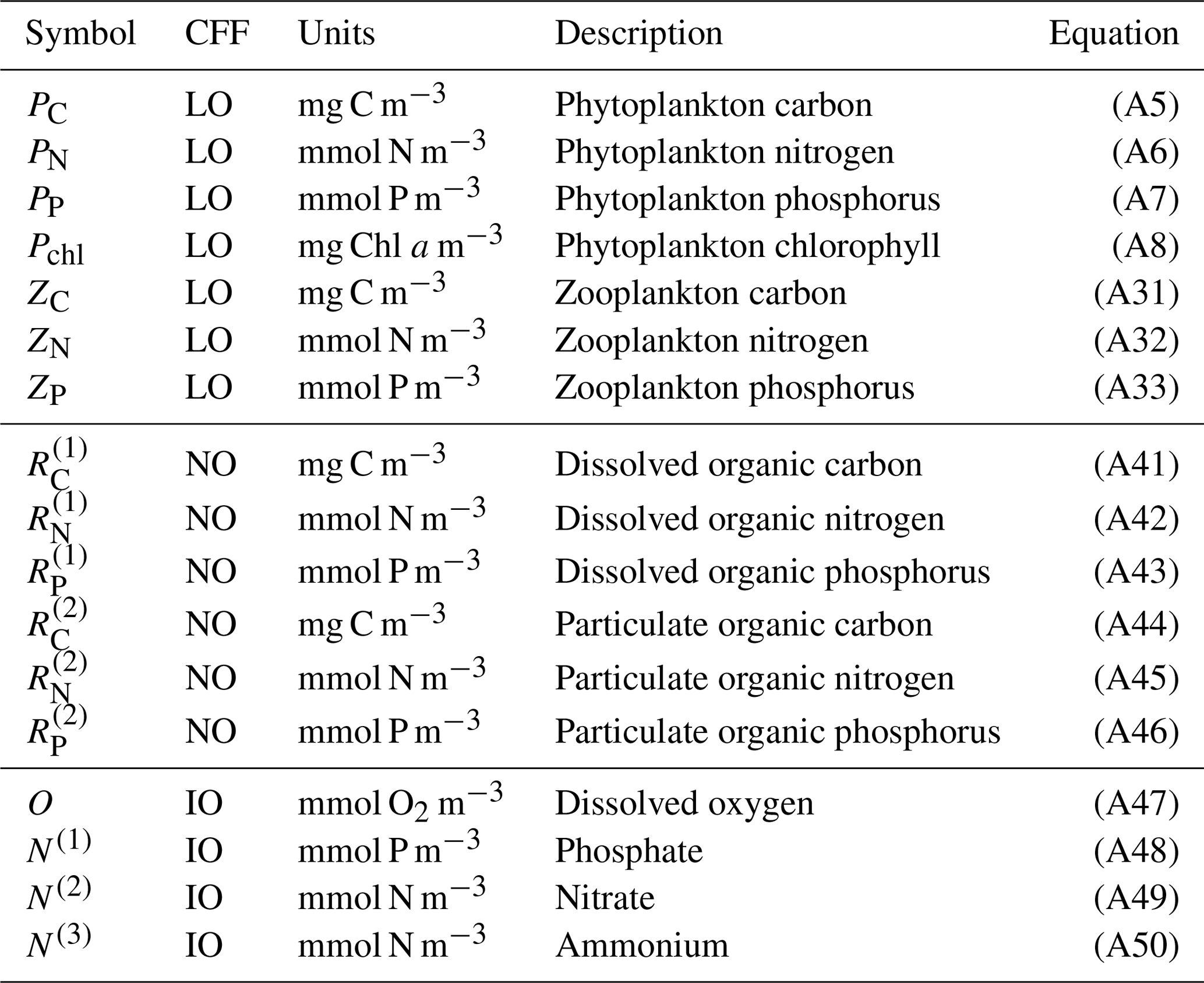
Figure 1 Schematic of the 17-state-equation BFM17 model. The dissolved organic matter, particulate organic matter, and living organic matter CFFs are each comprised of three chemical constituents (i.e., carbon, nitrogen, and phosphorus). The living organic CFF is further subdivided into phytoplankton and zooplankton living functional groups (LFGs).

3 Coupled physical–biogeochemical flux model

As a demonstration of BFM17 for predicting ocean biogeochemistry in oligotrophic pelagic zones, here we couple the model to a 1-D physical mixing parameterization and make comparisons with available observational data in the Sargasso Sea. In order to focus on the upper-thermocline, open-ocean regime for which BFM17 was developed, the physical model only extends 150 m in depth and diagnostically calculates diffusivity terms based upon prescribed temperature and salinity profiles from the observations. While a 1-D physical model is unlikely to resolve all processes relevant for biogeochemistry in the upper thermocline, we have made additions, such as large-scale general circulation and mesoscale eddy vertical velocities, as well as relaxation bottom boundary conditions for nutrient upwelling, to better represent missing processes.

For all equations here and in Appendix A, we adopt the same notation style used for BFM56 in Vichi et al. (2007), Mussap et al. (2016), and the BFM user manual (Vichi et al., 2013) for consistency and clarity. The coupled physical and BGC model is a time–depth model that integrates in time the generic equation for all biological state variables, denoted A_j, given by

$$\begin{array}{}\text{(1)}& \begin{array}{rl}{\displaystyle \frac{\partial A_j}{\partial t}}& ={\left.{\displaystyle \frac{\partial A_j}{\partial t}}\right|}_{\mathrm{bio}}-\left[W+W_{\mathrm{E}}+v^{\left(\mathrm{set}\right)}\right]{\displaystyle \frac{\partial A_j}{\partial z}}\\ & +{\displaystyle \frac{\partial }{\partial z}}\left(K_H{\displaystyle \frac{\partial A_j}{\partial z}}\right),\end{array}\end{array}$$

where A_j are the 17 state variables of BFM17, the first term on the right-hand side accounts for sources and sinks within each species due to biological and chemical reactions (as represented by the equations comprising BFM17 and outlined in Appendix A), W and W_E are the vertical velocities due to large-scale general circulation and mesoscale eddies, respectively, v^(set) is the settling velocity, and K_H is the vertical eddy diffusivity. Although the BFM17 formulation and model results are the primary focus of the present study, we also perform coupled physical–BGC simulations using BFM56 for comparison. Equation (1) applies to all 17 state variables in BFM17, as well as to all 56 state variables in BFM56. Consequently, the only differences between the biophysical models with BFM17 and BFM56 are the number of state variables being tracked and the equations used to calculate the biological forcing terms. The specific forms of Eq. (1) for each of the 17 species in BFM17 are discussed in Appendix A, and the specific forms of this equation for each of the 56 species in BFM56 were previously discussed in Vichi et al. (2007). The parameters used in BFM56 correspond to the values provided in Tables A3–A5 of Appendix A, with the remaining undefined parameters (since BFM56 includes many more model parameters than BFM17) based on values from Mussap et al. (2016).

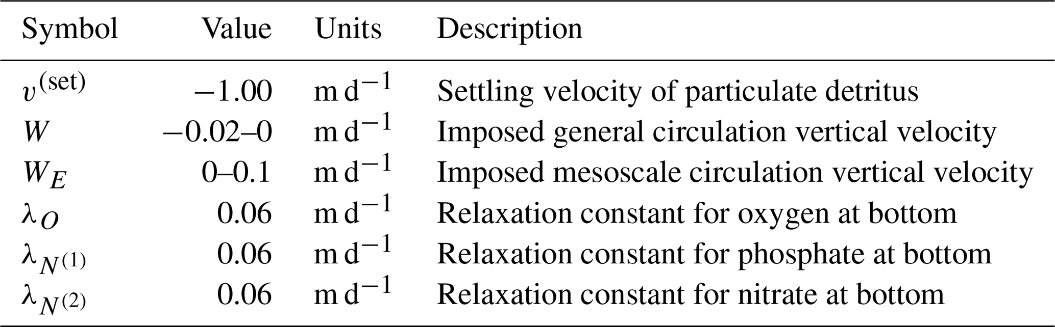
The range of values for W and W_E in Eq. (1) is included in Table 2 and the corresponding depth profiles are discussed in Sect. 4.3. The settling velocity, v^(set), in Eq. (1) is only non-zero for the three constituents of particulate organic matter, and its value is given in Table 2. We assume v^(set)=0 for zooplankton, since zooplankton actively swim and oppose their own sinking velocity. Finally, K_H in Eq. (1) is calculated by the model and is described in more detail later in this section.

Table 2 Values, units, and descriptions for parameters used in the combined physical–BFM17 model.

To obtain the complete 1-D biophysical model, BFM17 has been coupled with a modification of the three-dimensional (3-D) POM (Blumberg and Mellor, 1987) that considers only the vertical (specifically, the upper 150 m of the water column) and time dimensions; that is, the evolution of the system in the (z,t) space. It is well known that the primary calibration dimension in marine ocean biogeochemistry is along the vertical direction, as shown in several previous calibration and validation exercises (Vichi et al., 2003; Triantafyllou et al., 2003; Mussap et al., 2016).

The 1-D POM solver (POM-1D) is used to calculate the vertical structure of the two horizontal velocity components, denoted U and V, the potential temperature, T, salinity, S, density, ρ, turbulent kinetic energy, $q^{\mathrm{2}}/\mathrm{2}$, and mixing length scale, ℓ. In this model adaptation, vertical temperature and salinity profiles are imposed from given climatological monthly profiles obtained from observations, as previously done in Mussap et al. (2016) and Bianchi et al. (2005). POM-1D directly computes the time evolution of the horizontal velocity components, the turbulent kinetic energy and the mixing length scale, all of which are used to compute the turbulent diffusivity term, K_H, required in Eq. (1). In this configuration, POM-1D is called “diagnostic” since temperature and salinity are prescribed. Furthermore, pressure effects are neglected in the density equation and the buoyancy gradients and temperature are used in place of potential temperature since we consider only the upper water column.

A detailed description of POM can be found in Blumberg and Mellor (1987), and in the following we simply provide a description of the physical model and equations solved in POM-1D. In diagnostic mode, as used in the present study, POM-1D solves the momentum equations for U and V given by

$$\begin{array}{}\text{(2)}& {\displaystyle \frac{\partial U}{\partial t}}-fV={\displaystyle \frac{\partial }{\partial z}}\left(K_M{\displaystyle \frac{\partial U}{\partial z}}\right),\text{(3)}& {\displaystyle \frac{\partial V}{\partial t}}+fU={\displaystyle \frac{\partial }{\partial z}}\left(K_M{\displaystyle \frac{\partial V}{\partial z}}\right),\end{array}$$

where f=2Ωsin ϕ is the Coriolis force, Ω is the angular velocity of the Earth, and ϕ is the latitude. The vertical viscosity K_M and diffusivity K_H are calculated using the closure hypothesis of Mellor and Yamada (1982) as

$$\begin{array}{}\text{(4)}& {\displaystyle }{K}_M=ql{S}_M,\text{(5)}& {\displaystyle }{K}_H=ql{S}_H,\end{array}$$

where q is the turbulent velocity and S_H and S_M are stability functions written as

$$\begin{array}{}\text{(6)}& {\displaystyle }\begin{array}{r}{S}_M\left[\mathrm{1}-\mathrm{9}{A}_{\mathrm{1}}{A}_{\mathrm{2}}{G}_H\right]-S_H\left[(\mathrm{18}{A}_{\mathrm{1}}^{\mathrm{2}}+\mathrm{9}{A}_{\mathrm{1}}{A}_{\mathrm{2}})G_H\right]\\ =A_{\mathrm{1}}\left[\mathrm{1}-\mathrm{3}{C}_{\mathrm{1}}-\mathrm{6}{A}_{\mathrm{1}}/B_{\mathrm{1}}\right],\end{array}\text{(7)}& {\displaystyle }{S}_H\left[\mathrm{1}-(\mathrm{3}{A}_{\mathrm{2}}{B}_{\mathrm{2}}+\mathrm{18}{A}_{\mathrm{1}}{A}_{\mathrm{2}})G_H\right]=A_{\mathrm{2}}\left[\mathrm{1}-\mathrm{6}{A}_{\mathrm{1}}/B_{\mathrm{1}}\right].\end{array}$$

The coefficients in the above expressions are $(A_{\mathrm{1}},B_{\mathrm{1}},A_{\mathrm{2}},B_{\mathrm{2}},C_{\mathrm{1}})=(\mathrm{0.92},\mathrm{16.6},\mathrm{0.74},\mathrm{10.1},\mathrm{0.08})$, with

$$\begin{array}{}\text{(8)}& G_H={\displaystyle \frac{l^{\mathrm{2}}}{q^{\mathrm{2}}}}{\displaystyle \frac{g}{{\mathit{\rho }}_{\mathrm{0}}}}{\displaystyle \frac{\partial \mathit{\rho }}{\partial z}},\end{array}$$

where ρ₀=1025 kg m⁻³, g=9.81 m s⁻². Following Mellor (2001), G_H is limited to have a maximum value of 0.028. The equation of state relating ρ to T and S is non-linear (Mellor, 1991) and given by

$$\begin{array}{}\text{(9)}& \begin{array}{rl}\mathit{\rho }& =\mathrm{999.8}+(\mathrm{6.8}\times {\mathrm{10}}^{-\mathrm{2}}-\mathrm{9.1}\times {\mathrm{10}}^{-\mathrm{3}}T\\ & +\mathrm{1.0}\times {\mathrm{10}}^{-\mathrm{4}}{T}^{\mathrm{2}}-\mathrm{1.1}\times {\mathrm{10}}^{-\mathrm{6}}{T}^{\mathrm{3}}+\mathrm{6.5}\times {\mathrm{10}}^{-\mathrm{9}}{T}^{\mathrm{4}})T\\ & +(\mathrm{0.8}-\mathrm{4.1}\times {\mathrm{10}}^{-\mathrm{3}}T+\mathrm{7.6}\times {\mathrm{10}}^{-\mathrm{5}}{T}^{\mathrm{2}}\\ & -\mathrm{8.3}\times {\mathrm{10}}^{-\mathrm{7}}{T}^{\mathrm{3}}+\mathrm{5.4}\times {\mathrm{10}}^{-\mathrm{9}}{T}^{\mathrm{4}})S\\ & +(-\mathrm{5.7}\times {\mathrm{10}}^{-\mathrm{3}}+\mathrm{1.0}\times {\mathrm{10}}^{-\mathrm{4}}T\\ & -\mathrm{1.6}\times {\mathrm{10}}^{-\mathrm{6}}{T}^{\mathrm{2}})S^{\mathrm{1.5}}+\mathrm{4.8}\times {\mathrm{10}}^{-\mathrm{4}}{S}^{\mathrm{2}},\end{array}\end{array}$$

where the polynomial constants have been written only up to the first digit. For a more precise reproduction of these constants, the reader is referred to Mellor (1991). Finally, the governing equations solved to obtain the turbulence variables $q^{\mathrm{2}}/\mathrm{2}$ and ℓ are

$$\begin{array}{}\text{(10)}& {\displaystyle }\begin{array}{rl}{\displaystyle \frac{\partial }{\partial t}}\left({\displaystyle \frac{q^{\mathrm{2}}}{\mathrm{2}}}\right)& ={\displaystyle \frac{\partial }{\partial z}}\left[K_q{\displaystyle \frac{\partial }{\partial z}}\left({\displaystyle \frac{q^{\mathrm{2}}}{\mathrm{2}}}\right)\right]\\ & +K_M\left[{\left({\displaystyle \frac{\partial U}{\partial z}}\right)}^{\mathrm{2}}+{\left({\displaystyle \frac{\partial V}{\partial z}}\right)}^{\mathrm{2}}\right]\\ & +{\displaystyle \frac{g}{{\mathit{\rho }}_{\mathrm{0}}}}{K}_H{\displaystyle \frac{\partial \mathit{\rho }}{\partial z}}-{\displaystyle \frac{q^{\mathrm{3}}}{B_{\mathrm{1}}\mathrm{\ell }}},\end{array}\text{(11)}& {\displaystyle }\begin{array}{rl}{\displaystyle \frac{\partial }{\partial t}}\left(q^{\mathrm{2}}\mathrm{\ell }\right)& ={\displaystyle \frac{\partial }{\partial z}}\left[K_q{\displaystyle \frac{\partial }{\partial z}}\left(q^{\mathrm{2}}\mathrm{\ell }\right)\right]\\ & +E_{\mathrm{1}}\mathrm{\ell }{K}_M\left[{\left({\displaystyle \frac{\partial U}{\partial z}}\right)}^{\mathrm{2}}+{\left({\displaystyle \frac{\partial V}{\partial z}}\right)}^{\mathrm{2}}\right]\\ & +E_{\mathrm{1}}\mathrm{\ell }{\displaystyle \frac{g}{{\mathit{\rho }}_{\mathrm{0}}}}{K}_H{\displaystyle \frac{\partial \mathit{\rho }}{\partial z}}-{\displaystyle \frac{q^{\mathrm{3}}}{B_{\mathrm{1}}}}\stackrel{\mathrm{̃}}{W},\end{array}\end{array}$$

where K_q=κ K_H is the vertical diffusivity for turbulence variables, κ=0.4 is the von Karman constant, and $\stackrel{\mathrm{̃}}{W}=\left[\mathrm{1}+E_{\mathrm{2}}{\mathrm{\ell }}^{\mathrm{2}}/{\mathit{\kappa }}^{\mathrm{2}}(\mathrm{1}/|z|+\mathrm{1}/|z-H|{)}^{\mathrm{2}}\right]$ with $(E_{\mathrm{1}},E_{\mathrm{2}})=(\mathrm{1.8},\mathrm{1.33})$. In Eqs. (10) and (11), the time rate of change of the turbulence quantities is equal to the diffusion of turbulence (the first term on the right-hand side of both equations), the shear and buoyancy turbulence production (second and third terms), and the dissipation (the fourth term). This is a second-order turbulence closure model that was formulated by Mellor (2001) as a particular case of the Mellor and Yamada (1982) model for upper-ocean mixing.

Boundary conditions for the horizontal velocities $\mathit{U}=(U,V)$ and the turbulence quantities are

$$\begin{array}{}\text{(12)}& {\displaystyle }{K}_M{\displaystyle \frac{\partial \mathit{U}}{\partial z}}{|}_{z=\mathrm{0}}={\mathit{\tau }}_{\mathrm{w}},\text{(13)}& {\displaystyle }{K}_M{\displaystyle \frac{\partial \mathit{U}}{\partial z}}{|}_{z=z_{\mathrm{end}}}=\mathrm{0},\text{(14)}& {\displaystyle }{\left.\left(q^{\mathrm{2}},q^{\mathrm{2}}\mathrm{\ell }\right)\right|}_{z=\mathrm{0}}=\left(B_{\mathrm{1}}^{\mathrm{2}/\mathrm{3}}{\displaystyle \frac{\left|{\mathit{\tau }}_{\mathrm{w}}\right|}{C_{\mathrm{d}}}},\mathrm{0}\right),\text{(15)}& {\displaystyle }(q^{\mathrm{2}},q^{\mathrm{2}}\mathrm{\ell }){|}_{z=z_{\mathrm{end}}}=\mathrm{0},\end{array}$$

where ${\mathit{\tau }}_{\mathrm{w}}=C_{\mathrm{d}}\left|{\mathit{u}}_{\mathrm{w}}\right|{\mathit{u}}_{\mathrm{w}}$ is the surface wind stress, u_w is the surface wind vector, C_d is a constant drag coefficient chosen to be $\mathrm{2.5}\times {\mathrm{10}}^{-\mathrm{3}}$, and z=0 and z=z_end denote the locations of the surface and the greatest depth modeled, respectively.

For all variables except oxygen, surface boundary conditions for the coupled model variable A_j are

$$\begin{array}{}\text{(16)}& {\left.K_H{\displaystyle \frac{\partial A_j}{\partial z}}\right|}_{z=\mathrm{0}}=\mathrm{0}.\end{array}$$

By contrast, the surface boundary condition for oxygen has the form

$$\begin{array}{}\text{(17)}& {\left.K_H{\displaystyle \frac{\partial O}{\partial z}}\right|}_{z=\mathrm{0}}={\mathrm{\Phi }}_O,\end{array}$$

where Φ_O is the air–sea interface flux of oxygen computed according to Wanninkhof (1992, 2014). The bottom (i.e., greatest depth) boundary conditions for phytoplankton, zooplankton, dissolved organic matter, and particulate organic matter are

$$\begin{array}{}\text{(18)}& {\left.K_H{\displaystyle \frac{\partial A_j}{\partial z}}\right|}_{z=z_{\mathrm{end}}}=\mathrm{0}.\end{array}$$

This boundary condition was chosen since it allows removal of the scalar quantity A_j through the bottom boundary of the domain. This can be seen by integrating Eq. (1) over the boundary layer depth using the boundary condition above, giving

$$\begin{array}{}\text{(19)}& {\displaystyle \frac{\partial }{\partial t}}\underset{z=z_{\mathrm{end}}}{\overset{z=\mathrm{0}}{\int }}{A}_j\mathrm{d}z=\left[W+W_{\mathrm{E}}+v^{\left(\mathrm{set}\right)}\right]{\left.A_j\right|}_{z=z_{\mathrm{end}}},\end{array}$$

where the biological part of Eq. (1) has been neglected and the resulting temporal change in the integrated scalar A_j is negative since $\left|\right(W+W_{\mathrm{E}}\left)\right|<\left|v^{\left(\mathrm{set}\right)}\right|$, as shown in Table 2. For oxygen, phosphate, and nitrate, the bottom boundary conditions are

$$\begin{array}{}\text{(20)}& {\left.K_H{\displaystyle \frac{\partial A_j}{\partial z}}\right|}_{z=z_{\mathrm{end}}}={\mathit{\lambda }}_j\left({\left.A_j\right|}_{z=z_{\mathrm{end}}}-A_j^{*}\right),\end{array}$$

where λ_j and $A_j^{*}$ are the corresponding relaxation velocity and observed at-bottom boundary climatological field data value, respectively, of that species. Base values for the relaxation velocities are included in Table 2. Lastly, the bottom boundary condition for ammonium is

$$\begin{array}{}\text{(21)}& {\left.K_H{\displaystyle \frac{\partial N^{\left(\mathrm{3}\right)}}{\partial z}}\right|}_{z=z_{\mathrm{end}}}=\mathrm{0}.\end{array}$$

Since observations of ammonium concentration in the observational area are not available, this choice is based on the assumption that the nitrogen diffusive flux from depth to the surface (euphotic) layers occurs mostly in the form of a nitrate flux, consistent with the concepts of “new” and “regenerated” production, as described by Dugdale and Goering (1967) and Mulholland and Lomas (2008).

4 Field validation and calibration data

4.1 Study site description

Field data for calibration and validation of BFM17 are taken from the Bermuda Atlantic Time-series Study (BATS) (Steinberg et al., 2001) and the Bermuda Testbed Mooring (BTM) (Dickey et al., 2001) sites, which are located in the Sargasso Sea (31^∘40^′ N, 64^∘10^′ W) in the North Atlantic subtropical gyre. Both sites are a part of the US Joint Global Ocean Flux Study (JGOFS) program. Data have been collected from the BATS site since 1988 and from the BTM site since 1994.

Steinberg et al. (2001) provide an overview of the biogeochemistry in the general BATS and BTM area. Winter mixing allows nutrients to be brought up into the mixed layer, producing a phytoplankton bloom between January and March (winter mixed layer depth is typically 150–300 m). As thermal stratification intensifies over the summer months, this nutrient supply is cut off (summer mixed layer depth is typically 20 m). At this point, a subsurface chlorophyll maximum is observed near a depth of 100 m. Stoichiometric ratios of carbon, nitrate, and phosphate are often non-Redfield and, in contrast to many oligotrophic regimes, phosphate is the dominant limiting nutrient (Fanning, 1992; Michaels et al., 1993; Cavender-Bares et al., 2001; Steinberg et al., 2001; Ammerman et al., 2003; Martiny et al., 2013; Singh et al., 2015).

4.2 Data processing

The region encompassing the BATS and BTM sites is characterized as an open-ocean oligotrophic region that is phosphate limited. This region has thus been chosen for initial testing of BFM17 due to the prevalence of oligotrophic regimes in the open ocean and to demonstrate the ability of BFM17 to capture difficult non-Redfield ratio regimes (which occur in phosphate-limited regions). The BATS/BTM data have also been collected over many years, providing long time series for model calibration and validation.

Data from the BATS/BTM area are used in the present study for two purposes: (i) as initial, boundary, and forcing conditions for the POM-1D biophysical simulations with BFM17 and BFM56, and (ii) as target fields for validation of the simulations. In addition to the subsurface BATS data, we also use BTM surface data, such as the 10 m wind speed and photosynthetically active radiation (PAR). For each observational quantity, we compute monthly averages over 27 years for the BATS data and 23 years (not continuous) for the BTM data. Additionally, we interpolate the BATS data to a vertical grid with 1 m resolution. We subsequently smooth the interpolated data, using a robust locally estimated scatterplot smoothing (LOESS) method, to maintain a positive buoyancy gradient, thereby eliminating any spurious buoyancy-driven mixing due to interpolation and averaging.

Figure 2 shows the monthly climatological profiles of temperature and salinity from the BATS data (maximum mixed layer depth from the climatology is approximately 149 m, which was calculated based upon a 0.2 kg m⁻³ increase in density from the surface value), as well as the PAR and 10 m wind speed from the BTM data. The same monthly averaging, vertical interpolations, and smoothing used for the physical variables are also performed for biological variables, which largely serve as target fields for the validation of BFM17.

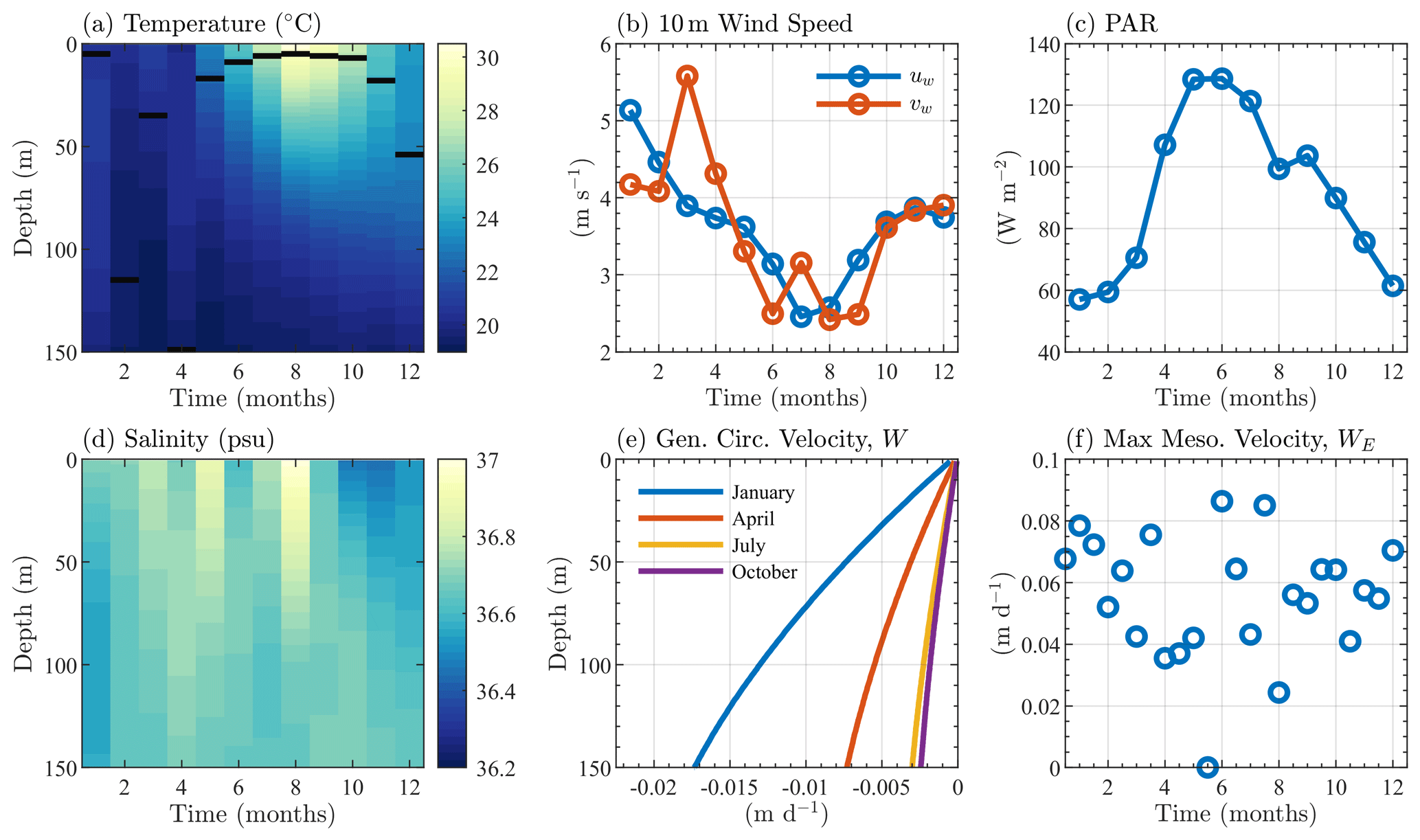
Figure 2 Sargasso Sea physical variables, showing climatological monthly averaged (a) temperature, (b) 10 m surface wind speed, (c) surface PAR, and (d) salinity. Panel (e) shows the mean seasonal general circulation velocity, W, and panel (f) shows the bimonthly maximum value of the mesoscale eddy velocity W_E. Monthly averaged mixed layer depths (defined as the depth at which the density is 0.2 kg m⁻³ greater than the surface density) are shown as black lines in panel (a).

4.3 Inputs to the physical model

The physical model computes density from the prescribed temperature and salinity, and surface wind stress from the 10 m wind speed; temperature, salinity, and wind speed are all provided by the BATS/BTM data. The model also uses these data in the turbulence closure to compute the turbulent viscosity and diffusivity. This diagnostic approach eliminates any drifts in temperature and salinity that might occur due to improper parameterizations of lateral mixing in a 1-D model, therefore providing greater reliability. In addition to the 10 m wind speed, temperature, and salinity, BFM requires monthly varying PAR at the surface. For all the monthly mean input datasets, a correction (Killworth, 1995) is applied. This correction is applied to the monthly averages to reduce the errors incurred by linearly interpolating monthly averages to the much shorter model time step.

We imposed both general circulation, W, and mesoscale eddy, W_E, vertical velocities in the simulations. The imposed vertical profiles of these velocities have been adapted from Bianchi et al. (2005), where the velocities are assumed to be zero at the surface and reach their maxima near the base of the Ekman layer, which is assumed to be at or below the bottom boundary of the simulations. The general large-scale upwelling or downwelling circulation, W, is due to Ekman pumping and is correspondingly given as

$$\begin{array}{}\text{(22)}& W=\widehat{\mathit{k}}\cdot \mathbf{\nabla }\times \left({\displaystyle \frac{{\mathit{\tau }}_{\mathrm{w}}}{\mathit{\rho }f}}\right),\end{array}$$

where $\widehat{\mathit{k}}$ denotes the unit vector in the vertical direction. The monthly average value and sign of the wind stress curl, ∇×τ_w, for the general BATS/BTM region is taken from the Scatterometer Climatology of Ocean Winds database (Risien and Chelton, 2008, 2011). The monthly value of W from Eq. (22) is then assumed to be the maximum, occurring at the base of the Ekman layer, for that particular month. Given the sign of the wind stress curl for the BATS/BTM region, a negative W was calculated, indicating general downwelling processes in this region. Seasonal profiles of W are shown in Fig. 2e.

Due to the prevalence of mesoscale eddies within the BATS/BTM region (Hua et al., 1985), which can provide episodic upwelling of nutrients to the upper water column, we also include an additional positive upwelling vertical velocity, W_E, which has a timescale of 15 d. The general profile of W_E is assumed to be the same as for W, with a value of zero at the surface and a maximum value at depth. However, there is no linear interpolation between each 15 d period, and the maximum magnitude of W_E is randomized between 0 and 0.1 m d⁻¹, as shown in Fig. 2f for each 15 d period.

4.4 Initial and boundary conditions

Although the BATS/BTM data include information on many biological variables, initial conditions for only 5 of the 17 species within BFM17 could be extracted from the data. Similarly to the temperature and salinity, the initial chlorophyll, particulate organic nitrogen, oxygen, nitrate, and phosphate were interpolated to a mesh with 1 m vertical grid spacing, averaged over the initial month of January, and smoothed vertically in space to give the initial profiles seen in Fig. 3a. The remaining 12-state-variable initial conditions were determined either through the adoption of the Redfield ratio $\mathrm{C}:\mathrm{N}:\mathrm{P}$ $\equiv \mathrm{106}:\mathrm{16}:\mathrm{1}$ (Redfield et al., 1963) or assuming a reasonably low initial value. Since the 1-D simulations were run to steady state over 10 years, memory of these initial states was assumed to be lost, with little effect on the results.

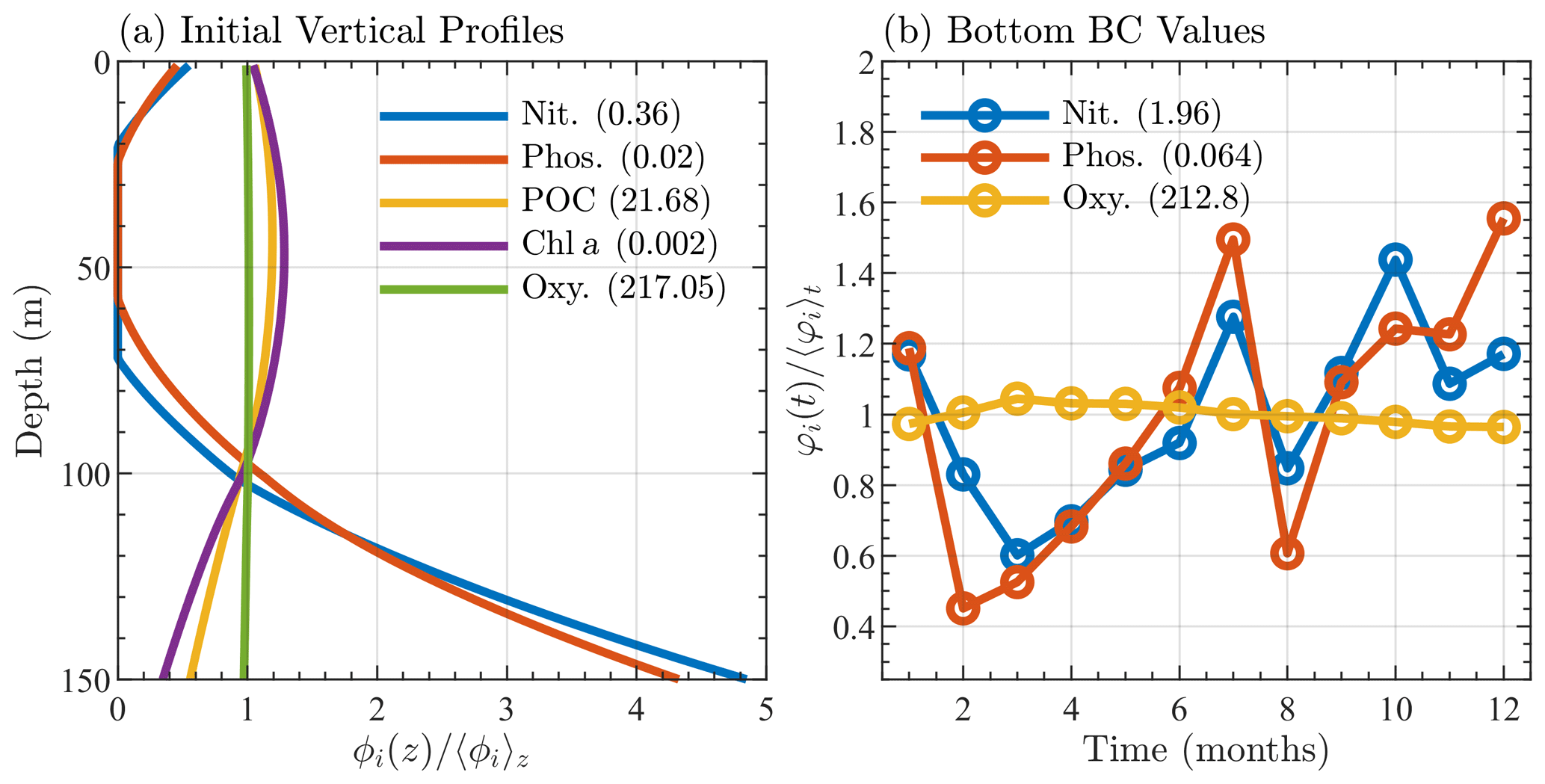
Figure 3 Sargasso Sea initial and boundary conditions showing (a) initial profiles of nitrate, phosphate, particulate organic carbon, chlorophyll, and oxygen, where each profile, denoted ϕ_i(z), is normalized by its depth averaged value, 〈ϕ_i〉_z, and (b) monthly bottom boundary conditions for nitrate, phosphate, and oxygen, where each quantity, φ_i(t), is normalized by its annual average value 〈φ_i〉_t. The depth and annual averaged values are shown in parentheses in the legends of each panel. Units are mmol N m⁻³ for nitrate, mmol P m⁻³ for phosphate, mg C m⁻³ for particulate organic carbon, mg Chl m⁻³ for chlorophyll, and mmol O m⁻³ for oxygen.

For the comparison of BFM17 to BFM56, the initial conditions for the additional state variables were calculated by splitting the total initial phytoplankton and zooplankton carbon values into equal amounts for all phytoplankton and zooplankton groups. The other state variables for each group were again calculated using the Redfield ratio. The initial bacteria distribution was defined by setting the column equal to a constant value.

In both simulations, the bottom boundary conditions for oxygen, nitrate, and phosphate species are based on observed BATS data. Values are taken at the next closest data point below the bottom boundary (at 150 m) and then averaged over the month. Figure 3b shows the monthly average bottom boundary conditions for each of the three species.

5 Model assessment results

The coupled BFM17-POM-1D model was run using the parameter values from Tables 2, A1, and A3–A5, which were decided on the basis of standard literature values (Vichi et al., 2007, 2003, 2013; Fiori et al., 2012). The simulations were allowed to run out to steady state, and multi-year monthly means were calculated as functions of depth for chlorophyll, oxygen, nitrate, phosphate, particulate organic nitrogen (PON), and net primary production (NPP), each of which was measured at the BATS/BTM site. The model PON is defined as the sum of nitrogen contained within the phytoplankton, zooplankton, and particulate detritus, and NPP is defined as the net phytoplankton carbon uptake (or gross primary production) minus phytoplankton respiration.

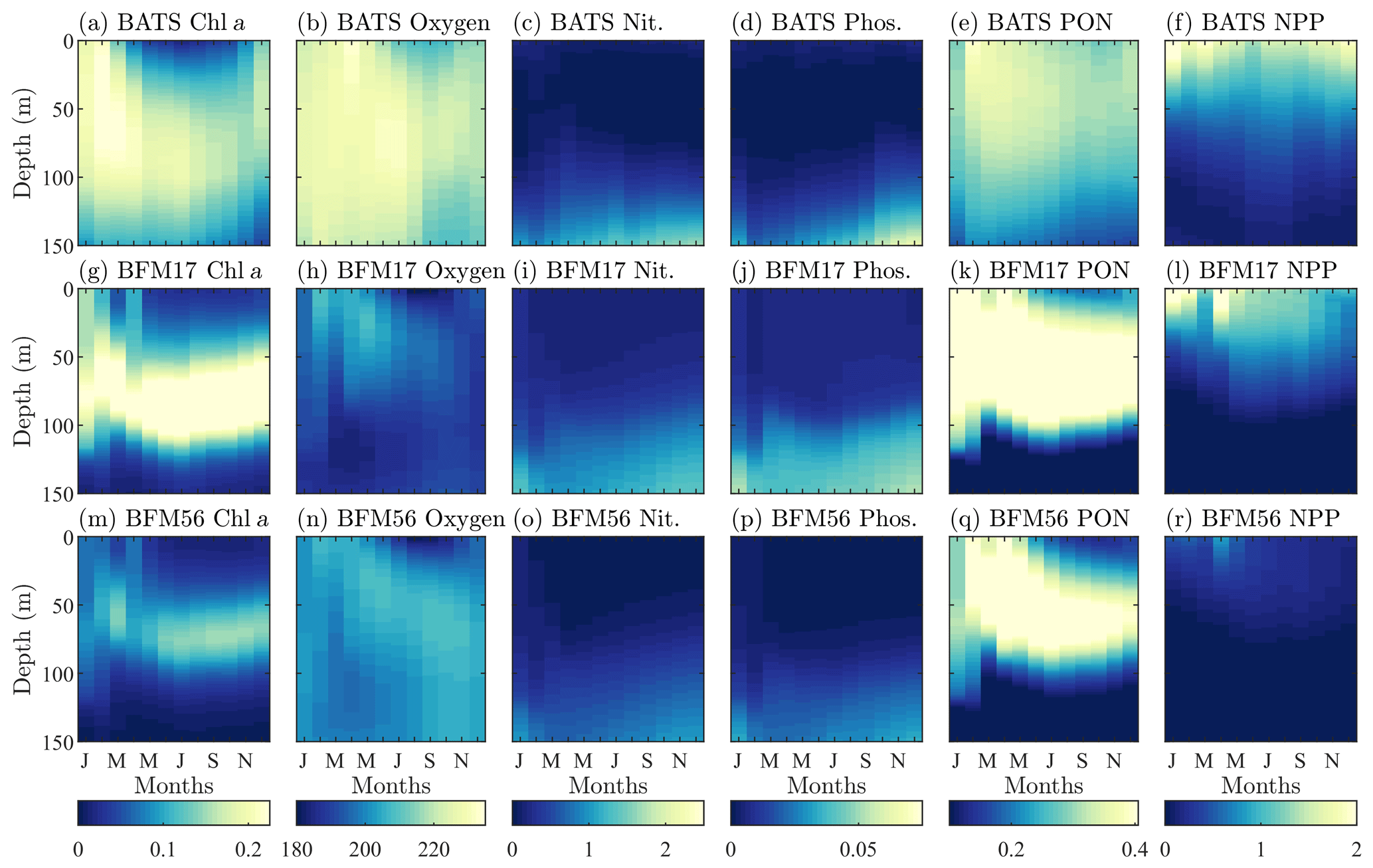
Figure 4 Comparison of target BATS fields (a–f) to BFM17 simulation results (g–l) and BFM56 simulation results (m–r) for (a ,g, m) chlorophyll (mg Chl a m⁻³), (b, h, n) oxygen (mmol O m⁻³), (c, i, o) nitrate (mmol N m⁻³), (d, j, p) phosphate (mmol P m⁻³), (e, k, q) particulate organic nitrogen (PON; mg N m⁻³), (f, l, r) and net primary production (NPP; mg C m⁻³ d⁻¹). Simulation plots are multi-year monthly averages of the last 3 years of a 10-year integration.

Figure 4 qualitatively compares the BATS data (top row) with the results from BFM17 (middle row). The model is able to capture the initial spring bloom between January and March brought on by physical entrainment of nutrients, the corresponding peak in net primary production and PON around the same time, and the subsequent subsurface chlorophyll maxima during the summer (evident in Fig. 4 as a larger chlorophyll concentration at depths close to 100 m during the summer months). The predicted oxygen levels are lower than observed values; however, the overall structure predicted by BFM17 is not completely dissimilar to that of the BATS oxygen field. These results are consistent with those from BFM56 (bottom row of Fig. 4), suggesting that the two models are in generally close agreement. Correlation coefficients between the two models are 0.85 for chlorophyll, 0.56 for oxygen, 0.99 for nitrate, 0.99 for phosphate, 0.95 for PON, and 0.97 for NPP. Differences in chlorophyll and oxygen are likely due to the removal in BFM17 of specific phytoplankton and zooplankton species in favor of general LFGs, to the removal of denitrification, and to the parameterization of remineralization using new closure terms that were calibrated to give reasonable agreement with the observational data.

As mentioned previously, oxygen is historically difficult to predict using BGC models of any complexity. It is likely that this is due, in part, to inaccuracies in the mixing parameterizations used in POM-1D and other physical models. For example, BFM17 struggles to accurately predict oxygen, in part, because the second-order mixing scheme of Mellor and Yamada (1982) lacks sufficient resolution of the winter mixing using just the monthly mean temperature and salinity. However, since it is often not included or presented at all in models of similar complexity to BFM17 (i.e., models reduced enough to reasonably couple to a high-fidelity, high-resolution physical model), studies that explore this hypothesis have been difficult to undertake. Thus, we include oxygen in BFM17 and present our results here to illustrate this exact point and to lend motivation to developing and using a model such as BFM17 to study the effects of physical processes missing from mixing parameterizations and how they can be better represented.

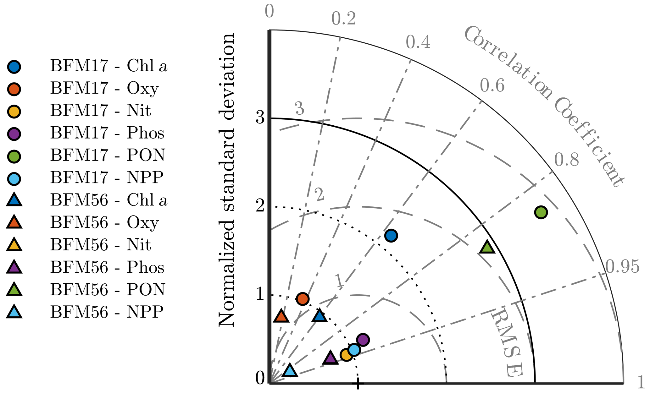
Figure 5 Taylor diagram showing the normalized standard deviation, correlation coefficient, and normalized root mean squared differences between the BFM17 output and the BATS target fields. Observations lie at (1,0). Radial deviations from observations correspond to the normalized root mean square error (RMSE), radial deviations from the origin correspond to the normalized standard deviation, and angular deviations from the vertical axis correspond to the correlation coefficient. BFM17 and BFM56 results are shown as colored circles and triangles, respectively (chlorophyll is indicated in blue, oxygen is indicated in orange, nitrate is indicated in yellow, phosphate is indicated in purple, PON is indicated in green, and NPP is indicated in cyan). Note that BFM56 nitrate and phosphate data points fall on top of one another (yellow and purple triangles).

To obtain a first indication of the performance of BFM17, a model assessment was performed for each target field. The same assessment was performed for BFM56 to compare the two models. The results are summarized by the Taylor diagram in Fig. 5. This diagram can be used to assess the extent of misfit between the models and observations by showing the normalized root mean square errors (RMSEs), normalized standard deviation, and the correlation coefficient between each of the model outputs and the BATS target fields.

The normalized RMSEs were calculated as ${\mathit{\epsilon }}_{\mathrm{rms}}/{\mathit{\sigma }}_{\mathrm{obs}}$, where ε_rms is the RMSE between the model and the observation fields and σ_obs is the standard deviation of the observation field. The normalized standard deviation was calculated as ${\mathit{\sigma }}_{\mathrm{mod}}/{\mathit{\sigma }}_{\mathrm{obs}}$, where σ_mod is the standard deviation of the model fields. The normalized RMSEs, normalized standard deviation, and the correlation coefficients each give an indication of the relative similarities in amplitude, variations in amplitude, and structure of each modeled field compared to the BATS target fields, respectively. For each variable, these statistics were calculated over all months and all depths shown in Fig. 4.

The Taylor diagram in Fig. 5 shows that BFM17 and BFM56 produce similar results. For most variables, errors in the amplitudes are within roughly one standard deviation of the observations. Additionally, the structures of the model fields for chlorophyll, nitrate, phosphate, PON, and NPP have high correlations with that of the BATS target fields. The correlation values range from 0.63 for chlorophyll to 0.94 for nitrate in BFM17 and from 0.60 for chlorophyll to 0.93 for phosphate and nitrate in BFM56. For BFM17, variabilities in amplitude for nitrate, phosphate, oxygen, and NPP are closest to those of the corresponding BATS target fields, while the chlorophyll and PON have too much variability. For BFM56, nitrate, phosphate, oxygen, and chlorophyll have similar variability in amplitude to the BATS data, while NPP and PON have too little and too much variability, respectively.

Table 3 provides a comparison of correlation coefficients and un-normalized RMSEs, calculated with respect to the observational fields, from BFM17 and BFM56, as well as from other models. Comparisons were only made to models that were calibrated using the same BATS/BTM data, employed some kind of parameter estimation technique, and reported correlation and RMSEs. Ayata et al. (2013) included six biological tracers, while both Fasham et al. (1990) and Spitz et al. (2001) included seven. The Spitz et al. (2001) study used data assimilation, while the Ayata et al. (2013) and Fasham et al. (1990) studies used only optimization to determine a select set of parameters. All models used climatological monthly mean forcing from the BATS region and reported climatological monthly means for their results. Care was taken to ensure that the same variable definition was compared between all models. Ayata et al. (2013) used a similar 1-D physical model to the one that was used here, while Spitz et al. (2001) and Fasham et al. (1990) used a time-dependent box model of the upper-ocean mixed layer. As such, correlations and RMSE values for comparison to Ayata et al. (2013) were computed over the entire domain (Ayata et al., 2013, calculated their metrics over the top 168 m of their domain). For comparison to Spitz et al. (2001) and Fasham et al. (1990), correlations and RMSEs were calculated only within the mixed layer (defined as the depth at which the density is 0.2 kg m⁻³ greater than the surface density) and are shown as separate columns in Table 3.

The correlation coefficients and RMSEs for both BFM17 and BFM56 are comparable to the Ayata et al. (2013) study for chlorophyll, while they outperform this study for nitrate, PON, and NPP. The Spitz et al. (2001) study, which used data assimilation and is therefore naturally more likely to perform better, does in fact do so for predictions of chlorophyll and nitrate. However, the nitrate correlation values for BFM17 and the Spitz et al. (2001) model are both high, although the latter model does have a lower RMSE value. As compared to the Spitz et al. (2001) model, BFM17 has higher correlation values for both PON and NPP but a larger RMSE for NPP. Lastly, both BFM17 and BFM56 outperform the Fasham et al. (1990) study for all fields for both correlation coefficient and RMSE values.

Table 3 Correlation coefficients (and RMSE in parenthesis) between BATS target fields and model data for BFM17, BFM56, and several example models of similar complexity. The first set of BFM columns is calculated over the entire water column, while the second set (denoted with “ML only”) is calculated over the monthly mixed layer depth only (defined as the depth at which the density is 0.2 kg m⁻³ greater than the surface density).

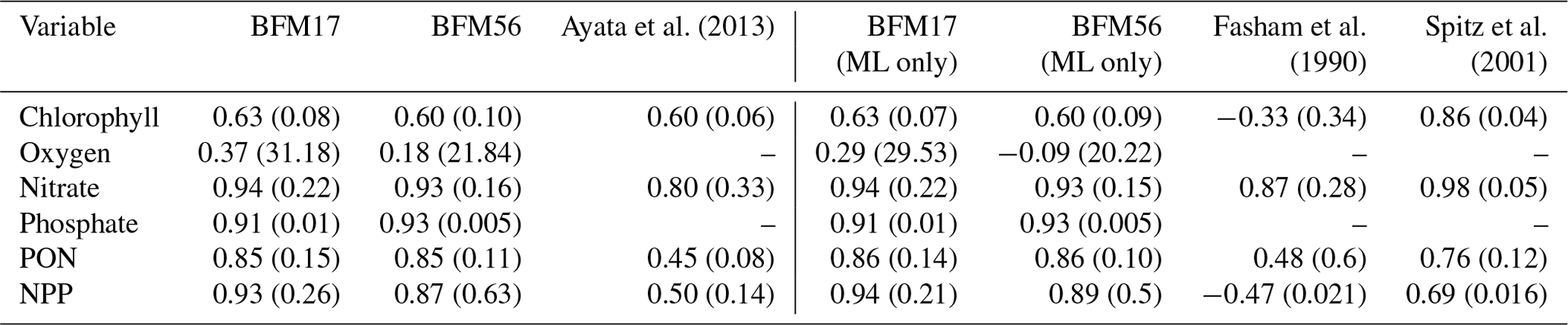
These results show that, with a relatively small increase in the number of biological tracers as compared to similar models, BFM17 is generally able to increase correlation coefficient values and decrease RMSE values for many of the target fields in comparison to similar models. Moreover, BFM17 approaches the accuracy of models that use data assimilation to improve agreement with the observations, such as the Spitz et al. (2001) model. The extra biological tracers in BFM17, as compared to the Ayata et al. (2013) and Fasham et al. (1990) models, account for variable intra- and extracellular nutrient ratios with the addition of phosphorus.

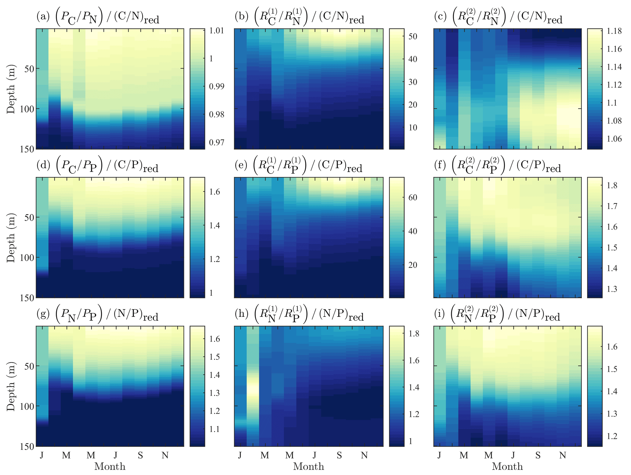
Figure 6 Fields of BFM17 constituent component ratios of carbon to nitrogen (a–c), carbon to phosphorous (d–f), and nitrogen to phosphorous (g–i) for phytoplankton (a, d, g), dissolved organic detritus (b, e, h), and particulate organic detritus (c, f, i). Each field is normalized by the respective Redfield ratio.

Finally, a key benefit of the chemical functional family approach used by BFM17 is the ability of the model to predict non-Redfield nutrient ratios. Figure 6 shows the constituent component ratios normalized by the respective Redfield ratios for BFM17. The figure includes the component ratios of carbon to nitrogen, carbon to phosphorous, and nitrogen to phosphorous for phytoplankton, dissolved organic matter (DOM), and POM. Zooplankton nutrient ratios were not included because the parameterization of the zooplankton relaxes the nutrient ratio back to a constant value. The normalized ratio values are uniform non-unity-valued fields.

Ultimately, Fig. 6 shows that BFM17 is able to capture the phosphate-limited dynamics that characterize the BATS/BTM region (Fanning, 1992; Michaels et al., 1993; Cavender-Bares et al., 2001; Steinberg et al., 2001; Ammerman et al., 2003; Martiny et al., 2013; Singh et al., 2015). In particular, Fig. 6 shows that all results comparing carbon or nitrogen to phosphorous for BFM17 produce normalized values greater than 1, where the normalization is carried out using the Redfield ratio (i.e., a normalized value greater than 1 indicates that the field is denominator limited). Figure 6 also shows that the ratios are not uniform for phytoplankton, DOM, and POM, with the ratios decreasing with depth as a result of the increased availability of nitrogen and phosphate.

6 Conclusions

In this study, we have presented a new upper-thermocline, open-ocean BGC model that is complex enough to capture open-ocean ecosystem dynamics within the Sargasso Sea region, yet reduced enough to integrate with a physical model with limited additional computational cost. The new model, named the Biogeochemical Flux Model 17 (BFM17), includes 17 state variables and expands upon more reduced BGC models by incorporating a phosphate equation and tracking dissolved oxygen, as well as variable intra- and extracellular nutrient ratios. BFM17 was developed primarily for use within high-resolution, high-fidelity 3-D physical models, such as LES, for process, parameterization, and parameter optimization studies, applications for which its more complex counterpart (BFM56) would be much too costly.

To calibrate and test the model, it was coupled to the 1-D Princeton Ocean Model (POM-1D) and forced using field data from the Bermuda Atlantic test site area. The full 56-state-variable Biogeochemical Flux Model (BFM56) was also run using the same forcing. Results were compared between the two models and all six of the BATS target fields – chlorophyll, oxygen, nitrate, phosphate, PON, and NPP – and a model skill assessment was performed, concluding that the BFM17 captures the subsurface chlorophyll maximum and bloom intensity observed in the BATS data and produces comparable results to BFM56. In comparison with similar studies using slightly less complex models, BFM17-POM-1D performs on par with, or better than, those studies.

In the future, a sensitivity study is necessary to assess the most sensitive model parameters, both in BFM17 as well as in the 1-D physical model. After identification of these most sensitive model parameters, an optimization can be performed to reduce discrepancies between the BATS observational biology fields and the corresponding model output fields. Additionally, it would be useful to study the efficacy of using BFM17 in a global context, to reproduce the ecology in other regions of the ocean, and its sensitivity under various physical forcing scenarios. Finally, BFM17 is now of a size that it can be efficiently integrated in high-resolution, high-fidelity 3-D simulations of the upper ocean, and future work will examine model results in this context.

Appendix A: BFM17 model equations

In the following, the detailed equations and their parameter values for each of the 17 state variables that comprise BFM17 are outlined. A summary of the 17 state variables is provided in Table 1 and a schematic of the CFFs and LFGs used in BFM17, along with their interactions, is shown in Fig. 1. It should be noted that for all BFM17 equations here, we adopt the same notation style used for BFM56 in Vichi et al. (2007), Mussap et al. (2016), and the BFM user manual (Vichi et al., 2013) for consistency and clarity.

A1 Environmental parameters

BFM17 is influenced by the environment through temperature and irradiance. Temperature directly affects all physiological processes and is represented in the model by introducing the non-dimensional parameter $f_j^{\left(T\right)}$ defined as

$$\begin{array}{}\text{(A1)}& f_j^{\left(T\right)}=Q_{\mathrm{10},j}^{(T-T^{*})/T^{*}},j=P,Z,\end{array}$$

where T^* is a base temperature and Q_10,j is a coefficient that may differ for the phytoplankton and zooplankton LFGs, denoted P_i and Z_i, respectively. Here, the subscript i is used to denote different chemical constituents (i.e., C, N, and P) and j is used to denote different LFGs. Base values used for T^* and Q_10,j are shown in Table A1. The model additionally employs a temperature-dependent nitrification parameter $f_{\mathrm{N}}^{\left(T\right)}$, which is defined similarly to Eq. (A1) as

$$\begin{array}{}\text{(A2)}& f_{\mathrm{N}}^{\left(T\right)}=Q_{\mathrm{10},\mathrm{N}}^{(T-T^{*})/T^{*}},\end{array}$$

where Q_10,N is given in Table A1.

Table A1 Symbols, values, units, and descriptions for environmental parameters within the BFM17 pelagic model.

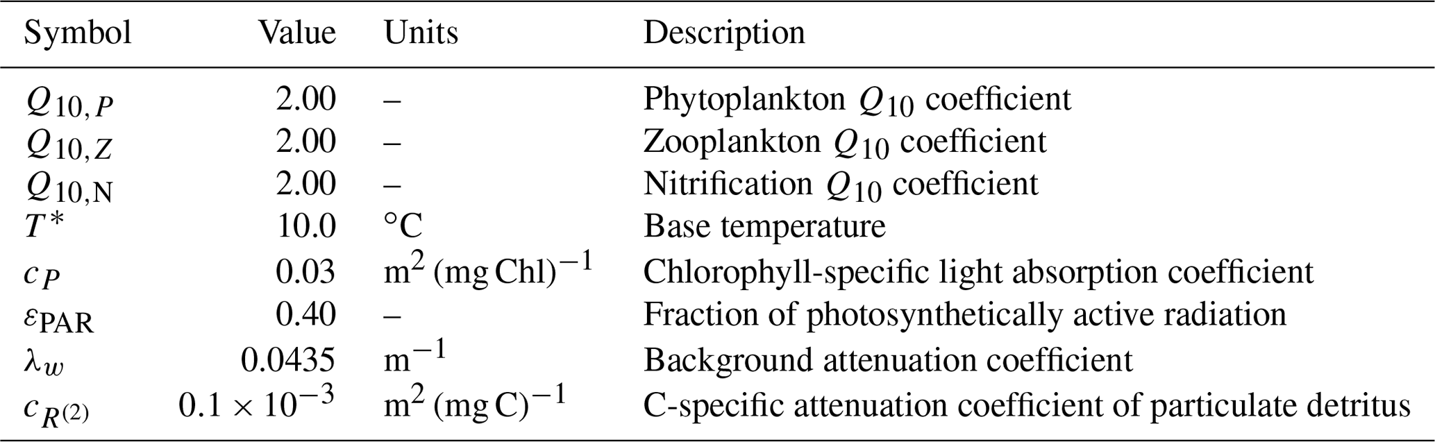
In contrast to temperature, irradiance only directly affects phytoplankton, serving as the primary energy source for phytoplankton growth and maintenance. Irradiance is a function of the incident solar radiation at the sea surface. Within BFM17, the amount of PAR at any given location z is parameterized according to the Beer–Lambert model as

$$\begin{array}{}\text{(A3)}& E_{\mathrm{PAR}}\left(z\right)={\mathit{\epsilon }}_{\mathrm{PAR}}{Q}_{\mathrm{S}}\exp \left[{\mathit{\lambda }}_{w}z+\underset{z}{\overset{\mathrm{0}}{\int }}{\mathit{\lambda }}_{\mathrm{bio}}\left(z^{\prime }\right)\mathrm{d}{z}^{\prime }\right],\end{array}$$

where Q_S is the shortwave surface irradiance flux, which is typically obtained from real-world measurements of the atmospheric radiative transfer, ε_PAR is the fraction of PAR within Q_S, λ_w is the background light extinction due to water, and λ_bio is the light extinction due to suspended biological particles. Values for ε_PAR and λ_w are given in Table A1. The extinction coefficient due to particulate matter, λ_bio, is dependent on phytoplankton chlorophyll, P_chl, and particulate detritus, $R_{\mathrm{C}}^{\left(\mathrm{2}\right)}$, and is written as

$$\begin{array}{}\text{(A4)}& {\mathit{\lambda }}_{\mathrm{bio}}=c_P{P}_{\mathrm{chl}}+c_{R^{\left(\mathrm{2}\right)}}{R}_{\mathrm{C}}^{\left(\mathrm{2}\right)},\end{array}$$

where c_P and $c_{R^{\left(\mathrm{2}\right)}}$ are the specific absorption coefficients of phytoplankton chlorophyll and particulate detritus, respectively, with values given in Table A1.

A2 Phytoplankton equations

The phytoplankton LFG in BFM17 is part of the living organic CFF and is composed of separate state variables for the constituents carbon, nitrogen, phosphorous, and chlorophyll, denoted P_C, P_N, P_P, and P_chl, respectively (see also Table 1). The governing equations for the constituent state variables are given by

• 1.

  the phytoplankton functional group in the living organic CFF, carbon constituent (state variable P_C):

  $$\begin{array}{}\text{(A5)}& \begin{array}{rl}{\left.{\displaystyle \frac{\partial P_{\mathrm{C}}}{\partial t}}\right|}_{\mathrm{bio}}& ={\left.{\displaystyle \frac{\partial P_{\mathrm{C}}}{\partial t}}\right|}_{{\mathrm{CO}}_{\mathrm{2}}}^{\mathrm{gpp}}-{\left.{\displaystyle \frac{\partial P_{\mathrm{C}}}{\partial t}}\right|}_{{\mathrm{CO}}_{\mathrm{2}}}^{\mathrm{rsp}}-{\left.{\displaystyle \frac{\partial P_{\mathrm{C}}}{\partial t}}\right|}_{R_{\mathrm{C}}^{\left(\mathrm{1}\right)}}^{\mathrm{lys}}\\ & -{\left.{\displaystyle \frac{\partial P_{\mathrm{C}}}{\partial t}}\right|}_{R_{\mathrm{C}}^{\left(\mathrm{2}\right)}}^{\mathrm{lys}}-{\left.{\displaystyle \frac{\partial P_{\mathrm{C}}}{\partial t}}\right|}_{R_{\mathrm{C}}^{\left(\mathrm{1}\right)}}^{\mathrm{exu}}-{\left.{\displaystyle \frac{\partial P_{\mathrm{C}}}{\partial t}}\right|}_{Z_{\mathrm{C}}}^{\mathrm{prd}},\end{array}\end{array}$$
• 2.

  the phytoplankton functional group in the living organic CFF, nitrogen constituent (state variable P_N):

  $$\begin{array}{}\text{(A6)}& \begin{array}{rl}{\left.{\displaystyle \frac{\partial P_{\mathrm{N}}}{\partial t}}\right|}_{\mathrm{bio}}& =max\left[\mathrm{0},{\left.{\displaystyle \frac{\partial P_{\mathrm{N}}}{\partial t}}\right|}_{N^{\left(\mathrm{2}\right)}}^{\mathrm{upt}}+{\left.{\displaystyle \frac{\partial P_{\mathrm{N}}}{\partial t}}\right|}_{N^{\left(\mathrm{3}\right)}}^{\mathrm{upt}}\right]\\ & -{\left.{\displaystyle \frac{\partial P_{\mathrm{N}}}{\partial t}}\right|}_{R_{\mathrm{N}}^{\left(\mathrm{1}\right)}}^{\mathrm{lys}}-{\left.{\displaystyle \frac{\partial P_{\mathrm{N}}}{\partial t}}\right|}_{R_{\mathrm{N}}^{\left(\mathrm{2}\right)}}^{\mathrm{lys}}-{\left.{\displaystyle \frac{\partial P_{\mathrm{N}}}{\partial t}}\right|}_{Z_{\mathrm{N}}}^{\mathrm{prd}},\end{array}\end{array}$$
• 3.

  the phytoplankton functional group in the living organic CFF, phosphorus constituent (state variable P_P):

  $$\begin{array}{}\text{(A7)}& \begin{array}{rl}{\left.{\displaystyle \frac{\partial P_{\mathrm{P}}}{\partial t}}\right|}_{\mathrm{bio}}& =max\left[\mathrm{0},{\left.{\displaystyle \frac{\partial P_{\mathrm{P}}}{\partial t}}\right|}_{N^{\left(\mathrm{1}\right)}}^{\mathrm{upt}}\right]-{\left.{\displaystyle \frac{\partial P_{\mathrm{P}}}{\partial t}}\right|}_{R_{\mathrm{P}}^{\left(\mathrm{1}\right)}}^{\mathrm{lys}}\\ & -{\left.{\displaystyle \frac{\partial P_{\mathrm{P}}}{\partial t}}\right|}_{R_{\mathrm{P}}^{\left(\mathrm{2}\right)}}^{\mathrm{lys}}-{\left.{\displaystyle \frac{\partial P_{\mathrm{P}}}{\partial t}}\right|}_{Z_{\mathrm{P}}}^{\mathrm{prd}},\end{array}\end{array}$$
• 4.

  the phytoplankton functional group in the living organic CFF, chlorophyll constituent (state variable P_chl):

  $$\begin{array}{}\text{(A8)}& {\left.{\displaystyle \frac{\partial P_{\mathrm{chl}}}{\partial t}}\right|}_{\mathrm{bio}}={\left.{\displaystyle \frac{\partial P_{\mathrm{chl}}}{\partial t}}\right|}^{\mathrm{syn}}-{\left.{\displaystyle \frac{\partial P_{\mathrm{chl}}}{\partial t}}\right|}^{\mathrm{loss}},\end{array}$$

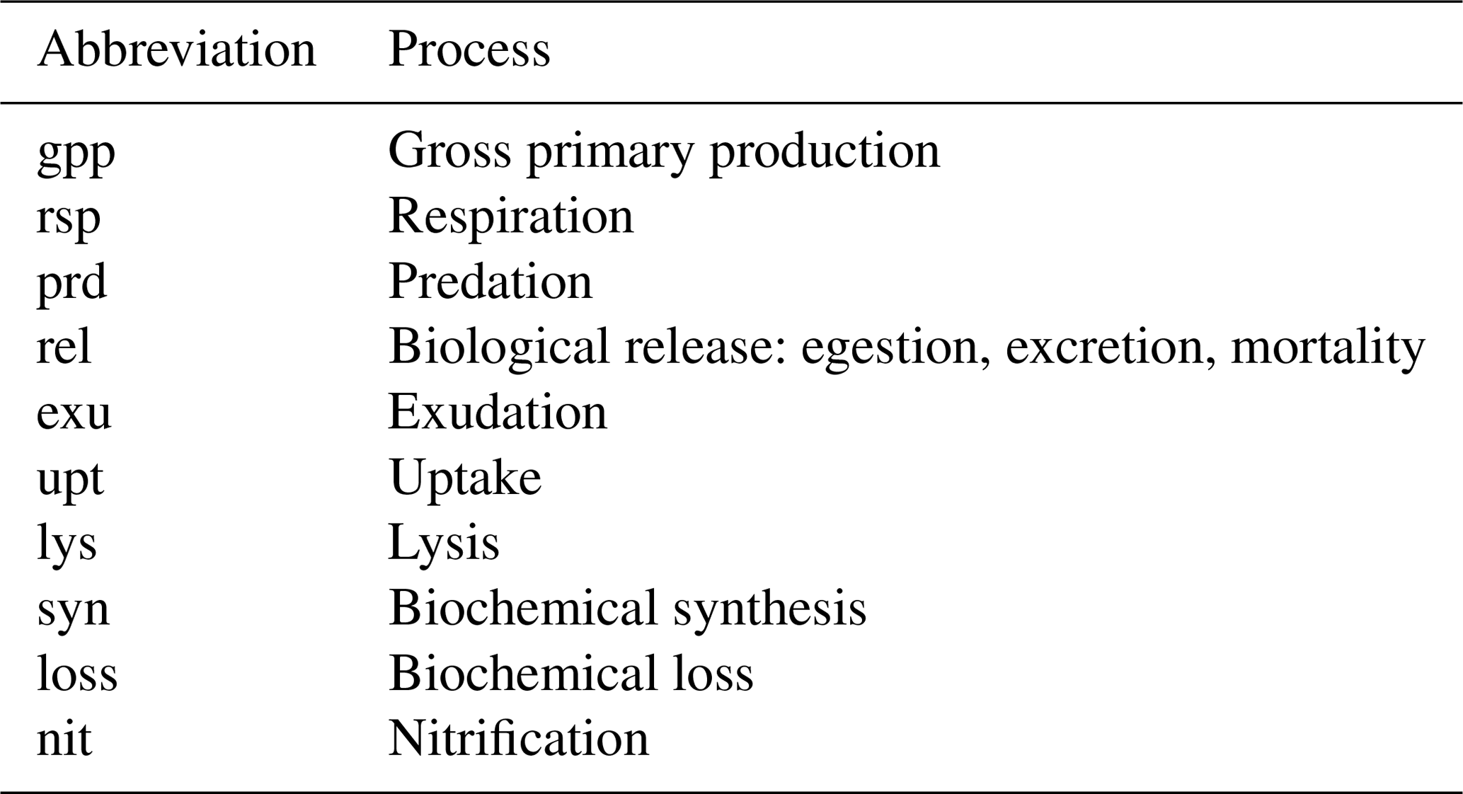
where the descriptions of each of the source and sink terms are provided in Table A2. The subscript “bio” on the left-hand-side terms indicates that these are the total rate expressions associated with all biological processes.

Table A2 List of abbreviations used to indicate physiological and ecological processes in the equations comprising the BFM17 pelagic model.

For the evolution of the phytoplankton carbon constituent given by Eq. (A5), gross primary production depends on the non-dimensional regulation factors for temperature and light as well as on the maximum photosynthetic growth rate and the phytoplankton carbon instantaneous concentration. This then gives

$$\begin{array}{}\text{(A9)}& {\left.{\displaystyle \frac{\partial P_{\mathrm{C}}}{\partial t}}\right|}_{{\mathrm{CO}}_{\mathrm{2}}}^{\mathrm{gpp}}=r_P^{\left(\mathrm{0}\right)}{f}_P^{\left(T\right)}{f}_P^{\left(E\right)}{P}_{\mathrm{C}},\end{array}$$

where $r_P^{\left(\mathrm{0}\right)}$ is the maximum photosynthetic rate for phytoplankton (reported in Table A3) and $f_P^{\left(T\right)}$ is the temperature-regulating factor for phytoplankton given by Eq. (A1). The term $f_P^{\left(E\right)}$ is the light regulation factor for phytoplankton, which is defined following Jassby and Platt (1976) as

$$\begin{array}{}\text{(A10)}& f_P^{\left(E\right)}=\mathrm{1}-\exp \left(-{\displaystyle \frac{E_{\mathrm{PAR}}}{E_{\mathrm{K}}}}\right),\end{array}$$

where E_PAR is defined in Eq. (A3) and E_K (the “optimal” irradiance) is given by

$$\begin{array}{}\text{(A11)}& E_{\mathrm{K}}=\left[{\displaystyle \frac{r_P^{\left(\mathrm{0}\right)}}{{\mathit{\alpha }}_{\mathrm{chl}}^{\left(\mathrm{0}\right)}}}\right]\left({\displaystyle \frac{P_{\mathrm{C}}}{P_{\mathrm{chl}}}}\right).\end{array}$$

The parameter ${\mathit{\alpha }}_{\mathrm{chl}}^{\left(\mathrm{0}\right)}$ is the maximum light utilization coefficient and is defined in Table A3.

Phytoplankton respiration is parameterized in Eq. (A5) as the sum of the basal respiration and activity respiration rates, namely

$$\begin{array}{}\text{(A12)}& \begin{array}{rl}{\left.{\displaystyle \frac{\partial P_{\mathrm{C}}}{\partial t}}\right|}_{{\mathrm{CO}}_{\mathrm{2}}}^{\mathrm{rsp}}& =b_P{f}_P^{\left(T\right)}{P}_{\mathrm{C}}\\ & +{\mathit{\gamma }}_P\left[{\left.{\displaystyle \frac{\partial P_{\mathrm{C}}}{\partial t}}\right|}_{{\mathrm{CO}}_{\mathrm{2}}}^{\mathrm{gpp}}-{\left.{\displaystyle \frac{\partial P_{\mathrm{C}}}{\partial t}}\right|}_{R_{\mathrm{C}}^{\left(\mathrm{1}\right)}}^{\mathrm{exu}}\right],\end{array}\end{array}$$

where b_P is the basal specific respiration rate, γ_P is the respired fraction of the gross primary production, the gross primary production term is given by Eq. (A9), and the exudation term is defined below in Eq. (A18). Values and descriptions for b_P and γ_P are given in Table A3.

Table A3 Phytoplankton parameters, values, units, and descriptions within the BFM17 pelagic model.

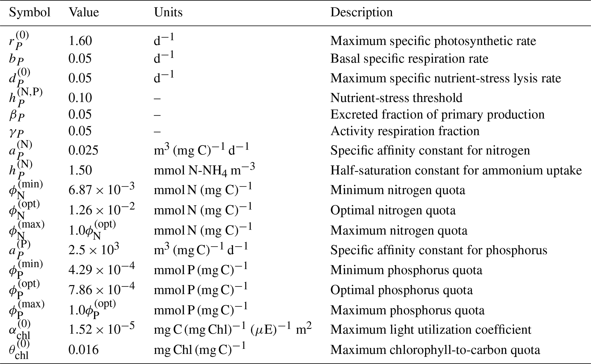
Both phytoplankton exudation and lysis, defined below, depend on a multiple nutrient limitation term $f_P^{(\mathrm{N},\mathrm{P})}$. This term allows for the internal storage of nutrients and depends on the respective nutrient limitation terms for both nitrate and phosphate. It is given by $f_P^{(\mathrm{N},\mathrm{P})}=min\left[f_P^{\left(\mathrm{N}\right)},f_P^{\left(\mathrm{P}\right)}\right]$, where

$$\begin{array}{}\text{(A13)}& {\displaystyle }{f}_P^{\left(\mathrm{N}\right)}& {\displaystyle }=min\left\{\mathrm{1},max\left[\mathrm{0},{\displaystyle \frac{P_{\mathrm{N}}/P_{\mathrm{C}}-{\mathit{\varphi }}_{\mathrm{N}}^{\left(\min \right)}}{{\mathit{\varphi }}_{\mathrm{N}}^{\left(\mathrm{opt}\right)}-{\mathit{\varphi }}_{\mathrm{N}}^{\left(\min \right)}}}\right]\right\},\text{(A14)}& {\displaystyle }{f}_P^{\left(\mathrm{P}\right)}& {\displaystyle }=min\left\{\mathrm{1},max\left[\mathrm{0},{\displaystyle \frac{P_{\mathrm{P}}/P_{\mathrm{C}}-{\mathit{\varphi }}_{\mathrm{P}}^{\left(\min \right)}}{{\mathit{\varphi }}_{\mathrm{P}}^{\left(\mathrm{opt}\right)}-{\mathit{\varphi }}_{\mathrm{P}}^{\left(\min \right)}}}\right]\right\}.\end{array}$$

The parameters ${\mathit{\varphi }}_{\mathrm{N}}^{\left(\mathrm{opt}\right)}$ and ${\mathit{\varphi }}_{\mathrm{P}}^{\left(\mathrm{opt}\right)}$ are the optimal phytoplankton quotas for nitrogen and phosphorus, respectively, while ${\mathit{\varphi }}_{\mathrm{N}}^{\left(\min \right)}$ and ${\mathit{\varphi }}_{\mathrm{P}}^{\left(\min \right)}$ are the minimum possible quotas, below which $f_P^{\left(\mathrm{N}\right)}$ and $f_P^{\left(\mathrm{P}\right)}$ are zero. Values for each of these parameters are included in Table A3.

Phytoplankton lysis includes all mortality due to mechanical, viral, and yeast cell disruption processes, and is partitioned between particulate and dissolved detritus. The internal cytoplasm of the cell is released to dissolved detritus, denoted by $R_i^{\left(\mathrm{1}\right)}$, while structural parts of the cell are released to particulate detritus, denoted by the state variable $R_i^{\left(\mathrm{2}\right)}$, where $i=\mathrm{C},\mathrm{N},\mathrm{P}$ (see also Table 1). The resulting lysis terms in Eqs. (A5)–(A7) are then given by

$$\begin{array}{}\text{(A15)}& {\displaystyle }\begin{array}{rl}& {\left.{\displaystyle \frac{\partial P_i}{\partial t}}\right|}_{R_i^{\left(\mathrm{1}\right)}}^{\mathrm{lys}}=\left[\mathrm{1}-{\mathit{\epsilon }}_P^{(\mathrm{N},\mathrm{P})}\right]\left[{\displaystyle \frac{h_P^{(\mathrm{N},\mathrm{P})}}{f_P^{(\mathrm{N},\mathrm{P})}+h_P^{(\mathrm{N},\mathrm{P})}}}{d}_P^{\left(\mathrm{0}\right)}{P}_i\right],\\ & i=\mathrm{C},\mathrm{N},\mathrm{P},\end{array}\text{(A16)}& {\displaystyle }\begin{array}{rl}& {\left.{\displaystyle \frac{\partial P_i}{\partial t}}\right|}_{R_i^{\left(\mathrm{2}\right)}}^{\mathrm{lys}}={\mathit{\epsilon }}_P^{(\mathrm{N},\mathrm{P})}\left[{\displaystyle \frac{h_P^{(\mathrm{N},\mathrm{P})}}{f_P^{(\mathrm{N},\mathrm{P})}+h_P^{(\mathrm{N},\mathrm{P})}}}{d}_P^{\left(\mathrm{0}\right)}{P}_i\right],\\ & i=\mathrm{C},\mathrm{N},\mathrm{P},\end{array}\end{array}$$

where $h_P^{(\mathrm{N},\mathrm{P})}$ is the nutrient-stress threshold and $d_P^{\left(\mathrm{0}\right)}$ is the maximum specific nutrient-stress lysis rate, both of which are given in Table A3. The term ${\mathit{\epsilon }}_P^{(\mathrm{N},\mathrm{P})}$ is a fraction that ensures nutrients within the structural parts of the cell, which are less degradable, are always released as particulate detritus. This fraction is determined by the expression

$$\begin{array}{}\text{(A17)}& {\mathit{\epsilon }}_P^{(\mathrm{N},\mathrm{P})}=min\left[\mathrm{1},{\displaystyle \frac{{\mathit{\varphi }}_{\mathrm{N}}^{\left(\min \right)}}{P_{\mathrm{N}}/P_{\mathrm{C}}}},{\displaystyle \frac{{\mathit{\varphi }}_{\mathrm{P}}^{\left(\min \right)}}{P_{\mathrm{P}}/P_{\mathrm{C}}}}\right],\end{array}$$

where ${\mathit{\varphi }}_{\mathrm{N}}^{\left(\min \right)}$ and ${\mathit{\varphi }}_{\mathrm{P}}^{\left(\min \right)}$ are given in Table A3.

If phytoplankton cannot equilibrate their fixed carbon with sufficient nutrients, this carbon is not assimilated and is instead released in the form of dissolved carbon, denoted by state variable $R_{\mathrm{C}}^{\left(\mathrm{1}\right)}$, in a process known as exudation. The exudation term in Eq. (A5) is parameterized as

$$\begin{array}{}\text{(A18)}& {\left.{\displaystyle \frac{\partial P_{\mathrm{C}}}{\partial t}}\right|}_{R_{\mathrm{C}}^{\left(\mathrm{1}\right)}}^{\mathrm{exu}}=\left\{{\mathit{\beta }}_P+(\mathrm{1}-{\mathit{\beta }}_P)\left[\mathrm{1}-f_P^{(\mathrm{N},\mathrm{P})}\right]\right\}{\left.{\displaystyle \frac{\partial P_{\mathrm{C}}}{\partial t}}\right|}_{{\mathrm{CO}}_{\mathrm{2}}}^{\mathrm{gpp}},\end{array}$$

where β_P is the excreted fraction of gross primary production, defined in Table A3, and the gross primary production term is again given by Eq. (A9).

The nutrient uptake of Eqs. (A6) and (A7) combines both the intracellular quota (i.e., Droop) and external concentration (i.e., Monod) approaches (Baretta-Bekker et al., 1997). The total phytoplankton uptake of nitrogen, represented by the combination of the two uptake terms in Eq. (A6), is the minimum of a diffusion-dependent uptake rate when internal nutrient quotas are low and a rate that is based upon balanced growth needs and any excess uptake, namely

$$\begin{array}{}\text{(A19)}& \begin{array}{rl}{\left.{\displaystyle \frac{\partial P_{\mathrm{N}}}{\partial t}}\right|}_{N^{(\mathrm{2},\mathrm{3})}}^{\mathrm{upt}}& =min\left\{a_P^{\left(\mathrm{N}\right)}\left[{\displaystyle \frac{h_P^{\left(\mathrm{N}\right)}}{h_P^{\left(\mathrm{N}\right)}+N^{\left(\mathrm{3}\right)}}}{N}^{\left(\mathrm{2}\right)}+N^{\left(\mathrm{3}\right)}\right]\right.P_{\mathrm{C}},\\ & {\mathit{\varphi }}_{\mathrm{N}}^{\left(\max \right)}{G}_P\\ & \left.+{\mathit{\nu }}_P\left[{\mathit{\varphi }}_{\mathrm{N}}^{\left(\max \right)}-{\displaystyle \frac{P_{\mathrm{N}}}{P_{\mathrm{C}}}}\right]P_{\mathrm{C}}\right\},\end{array}\end{array}$$

where $a_P^{\left(\mathrm{N}\right)}$ is the specific affinity for nitrogen, $h_P^{\left(\mathrm{N}\right)}$ is the half-saturation constant for ammonium uptake, and ${\mathit{\varphi }}_{\mathrm{N}}^{\left(\max \right)}$ is the maximum nitrogen quota; base values for these three parameters are given in Table A3. The net primary productivity G_P in Eq. (A19) is given as

$$\begin{array}{}\text{(A20)}& \begin{array}{rl}{G}_P& =max\left[\mathrm{0},{\left.{\displaystyle \frac{\partial P_{\mathrm{C}}}{\partial t}}\right|}_{{\mathrm{CO}}_{\mathrm{2}}}^{\mathrm{gpp}}-{\left.{\displaystyle \frac{\partial P_{\mathrm{C}}}{\partial t}}\right|}_{R_{\mathrm{C}}^{\left(\mathrm{1}\right)}}^{\mathrm{exu}}\right.\\ & \left.-{\left.{\displaystyle \frac{\partial P_{\mathrm{C}}}{\partial t}}\right|}_{{\mathrm{CO}}_{\mathrm{2}}}^{\mathrm{rsp}}-{\left.{\displaystyle \frac{\partial P_{\mathrm{C}}}{\partial t}}\right|}_{R_{\mathrm{C}}^{\left(\mathrm{1}\right)}}^{\mathrm{lys}}-{\left.{\displaystyle \frac{\partial P_{\mathrm{C}}}{\partial t}}\right|}_{R_{\mathrm{C}}^{\left(\mathrm{2}\right)}}^{\mathrm{lys}}\right].\end{array}\end{array}$$

The specific uptake rate ν_P appearing in Eq. (A19) is given by

$$\begin{array}{}\text{(A21)}& {\mathit{\nu }}_P=f_P^{\left(\mathrm{T}\right)}{r}_P^{\left(\mathrm{0}\right)}.\end{array}$$

It should be noted that only the sum of the two uptake terms, represented by Eq. (A19), is required in the governing equation for P_N given by Eq. (A6). However, in the governing equations for nitrate and ammonium, denoted N⁽²⁾ and N⁽³⁾ (see Table 1) that will be presented later, expressions are required for the individual uptake portions from nitrate and ammonium. When the total phytoplankton nitrogen uptake rate from Eq. (A19) is positive, the individual portions from nitrate and ammonium are determined by

$$\begin{array}{}\text{(A22)}& {\displaystyle }{\left.{\displaystyle \frac{\partial P_{\mathrm{N}}}{\partial t}}\right|}_{N^{\left(\mathrm{2}\right)}}^{\mathrm{upt}}& {\displaystyle }={\mathit{\epsilon }}_P{\left.{\displaystyle \frac{\partial P_{\mathrm{N}}}{\partial t}}\right|}_{N^{(\mathrm{2},\mathrm{3})}}^{\mathrm{upt}},\text{(A23)}& {\displaystyle }{\left.{\displaystyle \frac{\partial P_{\mathrm{N}}}{\partial t}}\right|}_{N^{\left(\mathrm{3}\right)}}^{\mathrm{upt}}& {\displaystyle }=\left(\mathrm{1}-{\mathit{\epsilon }}_P\right){\left.{\displaystyle \frac{\partial P_{\mathrm{N}}}{\partial t}}\right|}_{N^{(\mathrm{2},\mathrm{3})}}^{\mathrm{upt}},\end{array}$$

where the rates on the right-hand sides are obtained from Eq. (A19), and ε_P is given as

$$\begin{array}{}\text{(A24)}& {\mathit{\epsilon }}_P={\displaystyle \frac{s_{\mathrm{N}}{N}^{\left(\mathrm{2}\right)}}{N^{\left(\mathrm{3}\right)}+s_{\mathrm{N}}{N}^{\left(\mathrm{2}\right)}}}.\end{array}$$

The preference for ammonium is defined by the saturation function s_N and is given by

$$\begin{array}{}\text{(A25)}& s_{\mathrm{N}}={\displaystyle \frac{h_P^{\left(\mathrm{N}\right)}}{h_P^{\left(\mathrm{N}\right)}+N^{\left(\mathrm{3}\right)}}}.\end{array}$$

When the phytoplankton nitrogen uptake rate from Eq. (A19) is negative, however, the entire nitrogen uptake goes to the dissolved organic nitrogen pool, $R_{\mathrm{N}}^{\left(\mathrm{1}\right)}$ (see Eq. A42).

As with the uptake of nitrogen, phytoplankton uptake of phosphorus in Eq. (A7) is the minimum of a diffusion-dependent rate and a balanced growth/excess uptake rate. This uptake comes entirely from one pool and the uptake term in Eq. (A7) is correspondingly given by

$$\begin{array}{}\text{(A26)}& \begin{array}{rl}{\left.{\displaystyle \frac{\partial P_{\mathrm{P}}}{\partial t}}\right|}_{N^{\left(\mathrm{1}\right)}}^{\mathrm{upt}}& =min\left\{a_P^{\left(\mathrm{P}\right)}{N}^{\left(\mathrm{1}\right)}{P}_{\mathrm{C}},{\mathit{\varphi }}_{\mathrm{P}}^{\left(\max \right)}{G}_P\right.\\ & \left.+{\mathit{\nu }}_P\left[{\mathit{\varphi }}_{\mathrm{P}}^{\left(\max \right)}{P}_{\mathrm{C}}-P_{\mathrm{P}}\right]\right\},\end{array}\end{array}$$

where $a_P^{\left(\mathrm{P}\right)}$ is the specific affinity constant for phosphorous and ${\mathit{\varphi }}_{\mathrm{P}}^{\left(\max \right)}$ is the maximum phosphorous quota. Values for both parameters are given in Table A3. If the uptake rate is negative, the entire phosphorus uptake goes to the dissolved organic phosphorus pool, $R_{\mathrm{P}}^{\left(\mathrm{1}\right)}$.

Predation of phytoplankton within BFM17 is solely performed by zooplankton, and each of the predation terms appearing in Eqs. (A5)–(A7) are equal and opposite to the zooplankton predation terms, namely

$$\begin{array}{}\text{(A27)}& {\left.{\displaystyle \frac{\partial P_i}{\partial t}}\right|}_{Z_i}^{\mathrm{prd}}=-{\left.{\displaystyle \frac{\partial Z_i}{\partial t}}\right|}_{P_i}^{\mathrm{prd}},i=\mathrm{C},\mathrm{N},\mathrm{P}.\end{array}$$

Equations for the zooplankton predation terms are given in the next section.

Finally, phytoplankton chlorophyll, denoted P_chl with the rate equation given by Eq. (A8), contributes to the definition of the optimal irradiance value in Eq. (A11) and of the phytoplankton contribution to the extinction coefficient in Eq. (A4). The phytoplankton chlorophyll source term in Eq. (A8) is made up of only two terms: chlorophyll synthesis and loss. Net chlorophyll synthesis is a function of acclimation to light conditions, availability of nutrients, and turnover rate, and is given by

$$\begin{array}{}\text{(A28)}& \begin{array}{rl}{\left.{\displaystyle \frac{\partial P_{\mathrm{chl}}}{\partial t}}\right|}^{\mathrm{syn}}& ={\mathit{\rho }}_{\mathrm{chl}}\left(\mathrm{1}-{\mathit{\gamma }}_P\right)\left[{\left.{\displaystyle \frac{\partial P_{\mathrm{C}}}{\partial t}}\right|}_{{\mathrm{CO}}_{\mathrm{2}}}^{\mathrm{gpp}}-{\left.{\displaystyle \frac{\partial P_{\mathrm{C}}}{\partial t}}\right|}_{R_{\mathrm{C}}^{\left(\mathrm{1}\right)}}^{\mathrm{exu}}\right]\\ & -{\displaystyle \frac{P_{\mathrm{chl}}}{P_{\mathrm{C}}}}\left[{\left.{\displaystyle \frac{\partial P_{\mathrm{C}}}{\partial t}}\right|}_{R_{\mathrm{C}}^{\left(\mathrm{1}\right)}}^{\mathrm{lys}}+{\left.{\displaystyle \frac{\partial P_{\mathrm{C}}}{\partial t}}\right|}_{R_{\mathrm{C}}^{\left(\mathrm{2}\right)}}^{\mathrm{lys}}\right.\\ & \left.+{\left.{\displaystyle \frac{\partial P_{\mathrm{C}}}{\partial t}}\right|}_{{\mathrm{CO}}_{\mathrm{2}}}^{\mathrm{rsp}}\right],\end{array}\end{array}$$

where ρ_chl regulates the amount of chlorophyll in the phytoplankton cell and all other terms in the above expression have been defined previously. The term ρ_chl is computed according to a ratio between the realized photosynthetic rate (i.e., gross primary production) and the maximum potential photosynthesis (Geider et al., 1997), and is correspondingly given as

$$\begin{array}{}\text{(A29)}& \begin{array}{rl}{\mathit{\rho }}_{\mathrm{chl}}& ={\mathit{\theta }}_{\mathrm{chl}}^{\left(\mathrm{0}\right)}min\left\{\mathrm{1},{\displaystyle \frac{\left(\mathrm{1}-{\mathit{\gamma }}_P\right)}{{\mathit{\alpha }}_{\mathrm{chl}}^{\left(\mathrm{0}\right)}{E}_{\text{PAR}}{P}_{\mathrm{chl}}}}\left[{\left.{\displaystyle \frac{\partial P_{\mathrm{C}}}{\partial t}}\right|}_{{\mathrm{CO}}_{\mathrm{2}}}^{\mathrm{gpp}}\right.\right.\\ & \left.\left.-{\left.{\displaystyle \frac{\partial P_{\mathrm{C}}}{\partial t}}\right|}_{R_{\mathrm{C}}^{\left(\mathrm{1}\right)}}^{\mathrm{exu}}\right]\right\},\end{array}\end{array}$$

where ${\mathit{\theta }}_{\mathrm{chl}}^{\left(\mathrm{0}\right)}$ is the maximum chlorophyll-to-carbon quota and ${\mathit{\alpha }}_{\mathrm{chl}}^{\left(\mathrm{0}\right)}$ is the maximum light utilization coefficient, both of which can be found in Table A3. Chlorophyll loss in Eq. (A8) is simpler and is just a function of predation, where the amount of chlorophyll transferred back to the infinite sink is proportional to the carbon predated by zooplankton, giving

$$\begin{array}{}\text{(A30)}& {\left.{\displaystyle \frac{\partial P_{\mathrm{chl}}}{\partial t}}\right|}^{\mathrm{loss}}={\displaystyle \frac{P_{\mathrm{chl}}}{P_{\mathrm{C}}}}{\left.{\displaystyle \frac{\partial P_{\mathrm{C}}}{\partial t}}\right|}_{Z_{\mathrm{C}}}^{\mathrm{prd}}.\end{array}$$

A3 Zooplankton equations

The zooplankton LFG group in BFM17 is part of the living organic CFF and is composed of separate state variables for carbon, nitrogen, and phosphorous, denoted Z_C, Z_N, and Z_P, respectively (see also Table 1). The governing equations for the constituent state variables are given by

• 5.

  the zooplankton functional group in the living organic CFF, carbon constituent (state variable Z_C):

  $$\begin{array}{}\text{(A31)}& \begin{array}{rl}{\left.{\displaystyle \frac{\partial Z_{\mathrm{C}}}{\partial t}}\right|}_{\mathrm{bio}}& ={\left.{\displaystyle \frac{\partial Z_{\mathrm{C}}}{\partial t}}\right|}_{P_{\mathrm{C}}}^{\mathrm{prd}}-{\left.{\displaystyle \frac{\partial Z_{\mathrm{C}}}{\partial t}}\right|}_{{\mathrm{CO}}_{\mathrm{2}}}^{\mathrm{rsp}}\\ & -{\left.{\displaystyle \frac{\partial Z_{\mathrm{C}}}{\partial t}}\right|}_{R_{\mathrm{C}}^{\left(\mathrm{1}\right)}}^{\mathrm{rel}}-{\left.{\displaystyle \frac{\partial Z_{\mathrm{C}}}{\partial t}}\right|}_{R_{\mathrm{C}}^{\left(\mathrm{2}\right)}}^{\mathrm{rel}},\end{array}\end{array}$$
• 6.

  the zooplankton functional group in the living organic CFF, nitrogen constituent (state variable Z_N):

  $$\begin{array}{}\text{(A32)}& \begin{array}{rl}{\left.{\displaystyle \frac{\partial Z_{\mathrm{N}}}{\partial t}}\right|}_{\mathrm{bio}}& ={\left.{\displaystyle \frac{\partial Z_{\mathrm{N}}}{\partial t}}\right|}_{P_{\mathrm{N}}}^{\mathrm{prd}}-{\left.{\displaystyle \frac{\partial Z_{\mathrm{N}}}{\partial t}}\right|}_{R_{\mathrm{N}}^{\left(\mathrm{1}\right)}}^{\mathrm{rel}}\\ & -{\left.{\displaystyle \frac{\partial Z_{\mathrm{N}}}{\partial t}}\right|}_{R_{\mathrm{N}}^{\left(\mathrm{2}\right)}}^{\mathrm{rel}}-{\left.{\displaystyle \frac{\partial Z_{\mathrm{N}}}{\partial t}}\right|}_{N^{\left(\mathrm{3}\right)}}^{\mathrm{rel}},\end{array}\end{array}$$
• 7.

  the zooplankton functional group in the living organic CFF, phosphorus constituent (state variable Z_P):

  $$\begin{array}{}\text{(A33)}& \begin{array}{rl}{\left.{\displaystyle \frac{\partial Z_{\mathrm{P}}}{\partial t}}\right|}_{\mathrm{bio}}& ={\left.{\displaystyle \frac{\partial Z_{\mathrm{P}}}{\partial t}}\right|}_{P_{\mathrm{P}}}^{\mathrm{prd}}-{\left.{\displaystyle \frac{\partial Z_{\mathrm{P}}}{\partial t}}\right|}_{R_{\mathrm{P}}^{\left(\mathrm{1}\right)}}^{\mathrm{rel}}\\ & -{\left.{\displaystyle \frac{\partial Z_{\mathrm{P}}}{\partial t}}\right|}_{R_{\mathrm{P}}^{\left(\mathrm{2}\right)}}^{\mathrm{rel}}-{\left.{\displaystyle \frac{\partial Z_{\mathrm{P}}}{\partial t}}\right|}_{N^{\left(\mathrm{1}\right)}}^{\mathrm{rel}},\end{array}\end{array}$$

where, once more, descriptions of each of the source and sink terms are provided in Table A2.

Zooplankton predation of phytoplankton, which appears as the first term in each of Eqs. (A31)–(A33), primarily depends on the availability of phytoplankton and their capture efficiency, and is expressed as

$$\begin{array}{}\text{(A34)}& \begin{array}{rl}& {\left.{\displaystyle \frac{\partial Z_i}{\partial t}}\right|}_{P_{\mathrm{C}}}^{\mathrm{prd}}={\displaystyle \frac{P_i}{P_{\mathrm{C}}}}\left[f_Z^{\left(T\right)}{r}_Z^{\left(\mathrm{0}\right)}{\displaystyle \frac{P_{\mathrm{C}}}{P_{\mathrm{C}}+h_Z^{\left(\mathrm{F}\right)}\frac{(P_{\mathrm{C}}+{\mathit{\mu }}_Z)}{{\mathit{\delta }}_{Z,P}}}}{Z}_{\mathrm{C}}\right],\\ & i=\mathrm{C},\mathrm{N},\mathrm{P},\end{array}\end{array}$$

where $r_Z^{\left(\mathrm{O}\right)}$ is the potential specific growth rate, $h_Z^{\left(\mathrm{F}\right)}$ is the Michaelis constant for total food ingestion, and μ_Z is the feeding threshold. These parameters and their base values are included in Table A4. Here, $f_Z^{\left(T\right)}$ is the temperature-regulating factor for zooplankton growth given by Eq. (A1). The total food availability can be expressed as δ_Z,PP_C, where δ_Z,P is the prey availability of phytoplankton and is included in Table A4.

Zooplankton respiration is the sum of active and basal metabolism rates, where active respiration is the cost of nutrient ingestion, or predation. The resulting respiration rate is given by

$$\begin{array}{}\text{(A35)}& {\left.{\displaystyle \frac{\partial Z_{\mathrm{C}}}{\partial t}}\right|}_{{\mathrm{CO}}_{\mathrm{2}}}^{\mathrm{rsp}}=\left(\mathrm{1}-{\mathit{\eta }}_Z-{\mathit{\beta }}_Z\right){\left.{\displaystyle \frac{\partial Z_{\mathrm{C}}}{\partial t}}\right|}_{P_c}^{\mathrm{prd}}+b_Z{f}_Z^{\left(T\right)}{Z}_{\mathrm{C}},\end{array}$$

where η_Z is the assimilation efficiency, β_Z is the excreted fraction uptake, and b_Z is the basal specific respiration rate. All three parameters are included in Table A4.

Table A4 Zooplankton parameters, values, units, and descriptions within the BFM17 pelagic model.

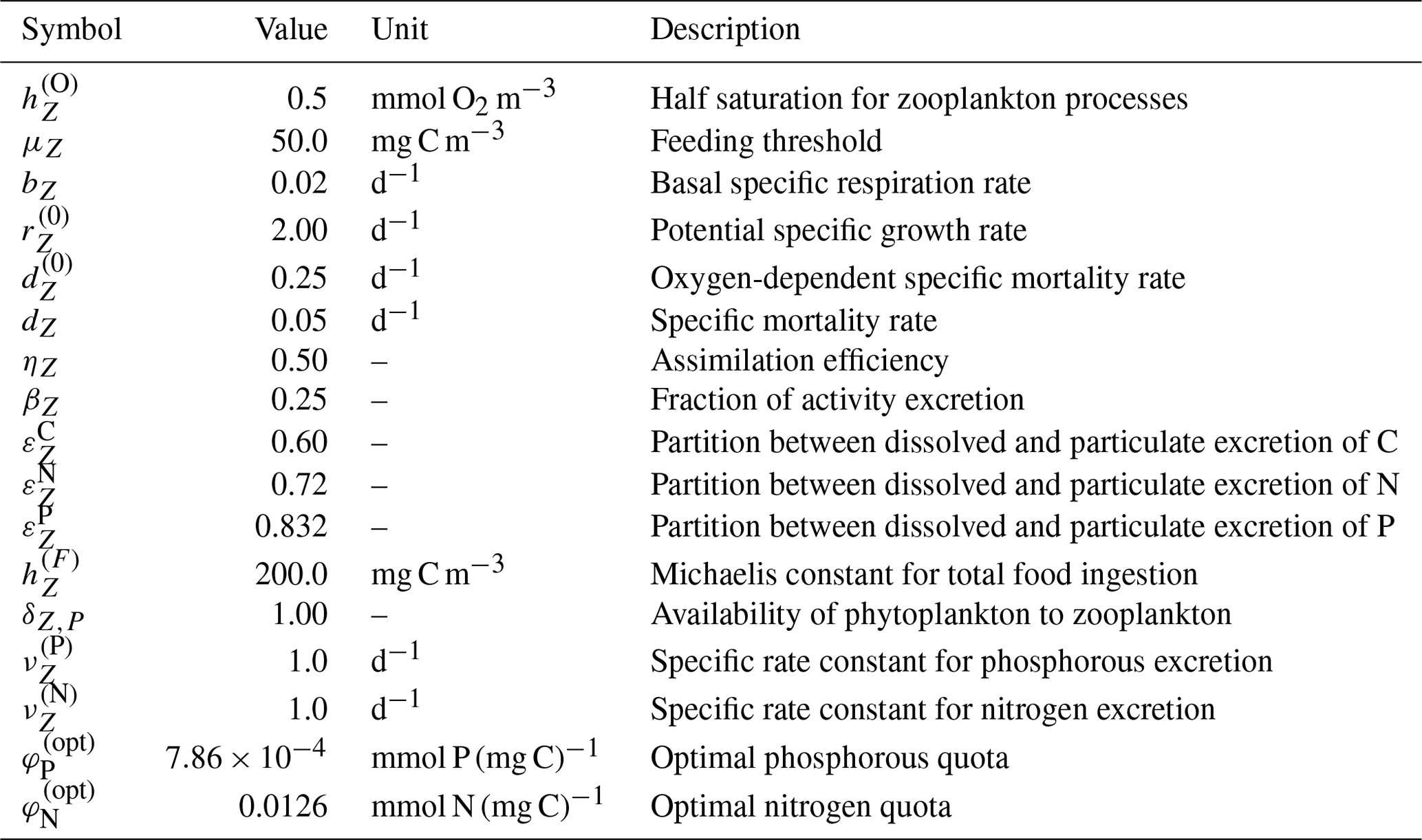
The biological release terms in Eqs. (A31)–(A33) are the sum of zooplankton excretion, egestion, and mortality. Excretion and egestion are the portions of ingested nutrients, resulting from predation, that have not been assimilated or used for respiration. Zooplankton mortality is parameterized as the sum of a constant mortality rate and an oxygen-dependent regulation factor given by

$$\begin{array}{}\text{(A36)}& f_A^{\left(\mathrm{O}\right)}={\displaystyle \frac{O}{O+h_A^{\left(\mathrm{O}\right)}}},\end{array}$$

where the subscript A is either Z for zooplankton or N for nitrification, O represents the oxygen constituents of the dissolved gas in the inorganic CFF, and $h_A^{\left(\mathrm{O}\right)}$ is the half-saturation coefficient for either zooplankton (subscript A=Z) processes or chemical (subscript A=N) processes given in Tables A4 and A5, respectively. The total biological release is then partitioned into particulate and dissolved organic matter, giving

$$\begin{array}{}\text{(A37)}& {\displaystyle }\begin{array}{rl}{\left.{\displaystyle \frac{\partial Z_i}{\partial t}}\right|}_{R_i^{\left(\mathrm{1}\right)}}^{\mathrm{rel}}& ={\mathit{\epsilon }}_Z^{\left(i\right)}\left\{{\mathit{\beta }}_Z{\left.{\displaystyle \frac{\partial Z_i}{\partial t}}\right|}_{P_i}^{\mathrm{prd}}+d_Z\right.\\ & +d_Z^{\left(\mathrm{0}\right)}\left.\left[\mathrm{1}-f_Z^{\left(\mathrm{O}\right)}\right]f_Z^{\left(T\right)}{Z}_i\right\},i=\mathrm{C},\mathrm{N},\mathrm{P},\end{array}\text{(A38)}& {\displaystyle }{\left.{\displaystyle \frac{\partial Z_i}{\partial t}}\right|}_{R_i^{\left(\mathrm{2}\right)}}^{\mathrm{rel}}=\left[\mathrm{1}-{\mathit{\epsilon }}_Z^{\left(i\right)}\right]{\left.{\displaystyle \frac{\partial Z_i}{\partial t}}\right|}_{R_i^{\left(\mathrm{1}\right)}}^{\mathrm{rel}},i=\mathrm{C},\mathrm{N},\mathrm{P},\end{array}$$

where ${\mathit{\epsilon }}_Z^{\left(i\right)}$ is the fraction excreted to the dissolved pool, d_Z is the specific mortality rate, and $d_Z^{\left(\mathrm{0}\right)}$ is the oxygen-dependent specific morality rate. Base values for each parameter are given in Table A4.

The zooplankton also excrete into the nutrient pools of phosphate, N⁽¹⁾, and ammonium, N⁽³⁾. These effects are represented by the final terms of Eqs. (A32) and (A33), which are parameterized by

$$\begin{array}{}\text{(A39)}& {\displaystyle }{\left.{\displaystyle \frac{\partial Z_{\mathrm{N}}}{\partial t}}\right|}_{N^{\left(\mathrm{3}\right)}}^{\mathrm{rel}}={\mathit{\nu }}_Z^{\left(\mathrm{N}\right)}\max \left[\mathrm{0},{\displaystyle \frac{Z_{\mathrm{N}}}{Z_{\mathrm{C}}}}-{\mathit{\phi }}_{\mathrm{N}}^{\left(\mathrm{opt}\right)}\right]Z_{\mathrm{N}},\text{(A40)}& {\displaystyle }{\left.{\displaystyle \frac{\partial Z_{\mathrm{P}}}{\partial t}}\right|}_{N^{\left(\mathrm{1}\right)}}^{\mathrm{rel}}={\mathit{\nu }}_Z^{\left(\mathrm{P}\right)}\max \left[\mathrm{0},{\displaystyle \frac{Z_{\mathrm{P}}}{Z_{\mathrm{C}}}}-{\mathit{\phi }}_{\mathrm{P}}^{\left(\mathrm{opt}\right)}\right]Z_{\mathrm{P}},\end{array}$$

where ${\mathit{\nu }}_Z^{\left(\mathrm{N}\right)}$ and ${\mathit{\nu }}_Z^{\left(\mathrm{P}\right)}$ are specific rate constants and ${\mathit{\phi }}_{\mathrm{N}}^{\left(\mathrm{opt}\right)}$ and ${\mathit{\phi }}_{\mathrm{P}}^{\left(\mathrm{opt}\right)}$ are the optimal zooplankton quotas for nitrogen and phosphorous, respectively. All four parameters are included in Table A4.

A4 Dissolved organic matter equations

The governing equations for the three constituents of dissolved organic matter are given by

• 8.

  dissolved matter in non-living organic CFF, carbon constituent [state variable $R_{\mathrm{C}}^{\left(\mathrm{1}\right)}$]:

  $$\begin{array}{}\text{(A41)}& \begin{array}{rl}{\left.{\displaystyle \frac{\partial R_{\mathrm{C}}^{\left(\mathrm{1}\right)}}{\partial t}}\right|}_{\mathrm{bio}}& ={\left.{\displaystyle \frac{\partial P_{\mathrm{C}}}{\partial t}}\right|}_{R_{\mathrm{C}}^{\left(\mathrm{1}\right)}}^{\mathrm{lys}}+{\left.{\displaystyle \frac{\partial P_{\mathrm{C}}}{\partial t}}\right|}_{R_{\mathrm{C}}^{\left(\mathrm{1}\right)}}^{\mathrm{exu}}\\ & +{\left.{\displaystyle \frac{\partial Z_{\mathrm{C}}}{\partial t}}\right|}_{R_{\mathrm{C}}^{\left(\mathrm{1}\right)}}^{\mathrm{rel}}-{\mathit{\alpha }}_{R^{\left(\mathrm{1}\right)}}^{\left({\mathrm{sink}}_{\mathrm{C}}\right)}{R}_{\mathrm{C}}^{\left(\mathrm{1}\right)},\end{array}\end{array}$$
• 9.

  dissolved matter in non-living organic CFF, nitrogen constituent [state variable $R_{\mathrm{N}}^{\left(\mathrm{1}\right)}$]:

  $$\begin{array}{}\text{(A42)}& \begin{array}{rl}{\left.{\displaystyle \frac{\partial R_{\mathrm{N}}^{\left(\mathrm{1}\right)}}{\partial t}}\right|}_{\mathrm{bio}}& ={\left.{\displaystyle \frac{\partial P_{\mathrm{N}}}{\partial t}}\right|}_{R_{\mathrm{N}}^{\left(\mathrm{1}\right)}}^{\mathrm{lys}}+{\left.{\displaystyle \frac{\partial Z_{\mathrm{N}}}{\partial t}}\right|}_{R_{\mathrm{N}}^{\left(\mathrm{1}\right)}}^{\mathrm{rel}}\\ & -min\left[\mathrm{0},{\left.{\displaystyle \frac{\partial P_{\mathrm{N}}}{\partial t}}\right|}_{N^{\left(\mathrm{2}\right)}}^{\mathrm{upt}}+{\left.{\displaystyle \frac{\partial P_{\mathrm{N}}}{\partial t}}\right|}_{N^{\left(\mathrm{3}\right)}}^{\mathrm{upt}}\right]\\ & -{\mathit{\zeta }}_{N^{\left(\mathrm{3}\right)}}{R}_{\mathrm{N}}^{\left(\mathrm{1}\right)},\end{array}\end{array}$$
• 10.

  dissolved matter in non-living organic CFF, phosphorus constituent [state variable $R_{\mathrm{P}}^{\left(\mathrm{1}\right)}$]:

  $$\begin{array}{}\text{(A43)}& \begin{array}{rl}{\left.{\displaystyle \frac{\partial R_{\mathrm{P}}^{\left(\mathrm{1}\right)}}{\partial t}}\right|}_{\mathrm{bio}}& ={\left.{\displaystyle \frac{\partial P_{\mathrm{P}}}{\partial t}}\right|}_{R_{\mathrm{P}}^{\left(\mathrm{1}\right)}}^{\mathrm{lys}}+{\left.{\displaystyle \frac{\partial Z_{\mathrm{P}}}{\partial t}}\right|}_{R_{\mathrm{P}}^{\left(\mathrm{1}\right)}}^{\mathrm{rel}}\\ & -min\left[\mathrm{0},{\left.{\displaystyle \frac{\partial P_{\mathrm{P}}}{\partial t}}\right|}_{N^{\left(\mathrm{1}\right)}}^{\mathrm{upt}}\right]-{\mathit{\zeta }}_{N^{\left(\mathrm{1}\right)}}{R}_{\mathrm{P}}^{\left(\mathrm{1}\right)}.\end{array}\end{array}$$

All terms except for the last terms in each of these equations, representing remineralization, have been defined in previous sections. Remineralization of dissolved organic matter by bacteria is parameterized within BFM17 as a rate that is proportional to the local concentration of that dissolved constituent. In Eq. (A41), remineralization is parameterized as ${\mathit{\alpha }}_{R^{\left(\mathrm{1}\right)}}^{\left({\mathrm{sink}}_{\mathrm{C}}\right)}{R}_{\mathrm{C}}^{\left(\mathrm{1}\right)}$, where ${\mathit{\alpha }}_{R^{\left(\mathrm{1}\right)}}^{\left({\mathrm{sink}}_{\mathrm{C}}\right)}$ is a constant that controls the rate at which dissolved carbon is remineralized and returned to the pool of carbon; this constant is given in Table A5. In Eqs. (A42) and (A43), remineralization is represented by the parameters ${\mathit{\zeta }}_{N^{\left(\mathrm{3}\right)}}$ and ${\mathit{\zeta }}_{N^{\left(\mathrm{1}\right)}}$, which are the specific remineralization rates of dissolved ammonium and phosphate, respectively. These rates are also included in Table A5.

Table A5 Values, units, and descriptions for dissolved organic matter, particulate organic matter, and nutrient parameters within the BFM17 pelagic model.

A5 Particulate organic matter equations

The governing equations for the three constituents of particulate organic matter are given by

• 11.

  particulate matter in non-living organic CFF, carbon constituent [state variable $R_{\mathrm{C}}^{\left(\mathrm{2}\right)}$]:

  $$\begin{array}{}\text{(A44)}& \begin{array}{rl}{\left.{\displaystyle \frac{\partial R_{\mathrm{C}}^{\left(\mathrm{2}\right)}}{\partial t}}\right|}_{\mathrm{bio}}& ={\left.{\displaystyle \frac{\partial P_{\mathrm{C}}}{\partial t}}\right|}_{R_{\mathrm{C}}^{\left(\mathrm{2}\right)}}^{\mathrm{lys}}+{\left.{\displaystyle \frac{\partial Z_{\mathrm{C}}}{\partial t}}\right|}_{R_{\mathrm{C}}^{\left(\mathrm{2}\right)}}^{\mathrm{rel}}\\ & -{\mathit{\alpha }}_{R^{\left(\mathrm{2}\right)}}^{\left({\mathrm{sink}}_{\mathrm{C}}\right)}{R}_{\mathrm{C}}^{\left(\mathrm{2}\right)},\end{array}\end{array}$$
• 12.

  particulate matter in non-living organic CFF, nitrogen constituent [state variable $R_{\mathrm{N}}^{\left(\mathrm{2}\right)}$]:

  $$\begin{array}{}\text{(A45)}& \begin{array}{rl}{\left.{\displaystyle \frac{\partial R_{\mathrm{N}}^{\left(\mathrm{2}\right)}}{\partial t}}\right|}_{\mathrm{bio}}& ={\left.{\displaystyle \frac{\partial P_{\mathrm{N}}}{\partial t}}\right|}_{R_{\mathrm{N}}^{\left(\mathrm{2}\right)}}^{\mathrm{lys}}+{\left.{\displaystyle \frac{\partial Z_{\mathrm{N}}}{\partial t}}\right|}_{R_{\mathrm{N}}^{\left(\mathrm{2}\right)}}^{\mathrm{rel}}\\ & -{\mathit{\xi }}_{N^{\left(\mathrm{3}\right)}}{R}_{\mathrm{N}}^{\left(\mathrm{2}\right)},\end{array}\end{array}$$
• 13.

  particulate matter in non-living organic CFF, phosphorus constituent [state variable $R_{\mathrm{P}}^{\left(\mathrm{2}\right)}$]:

  $$\begin{array}{}\text{(A46)}& {\left.{\displaystyle \frac{\partial R_{\mathrm{P}}^{\left(\mathrm{2}\right)}}{\partial t}}\right|}_{\mathrm{bio}}={\left.{\displaystyle \frac{\partial P_{\mathrm{P}}}{\partial t}}\right|}_{R_{\mathrm{P}}^{\left(\mathrm{2}\right)}}^{\mathrm{lys}}+{\left.{\displaystyle \frac{\partial Z_{\mathrm{P}}}{\partial t}}\right|}_{R_{\mathrm{P}}^{\left(\mathrm{2}\right)}}^{\mathrm{rel}}-{\mathit{\xi }}_{N^{\left(\mathrm{1}\right)}}{R}_{\mathrm{P}}^{\left(\mathrm{2}\right)}.\end{array}$$

Once again, all terms except for the final remineralization terms in each equation have been defined in previous sections. Remineralization of particular organic matter by bacteria is parameterized within BFM17 as a rate that is proportional to the local concentration of that particulate constituent. In Eq. (A44), remineralization is parameterized by ${\mathit{\alpha }}_{R^{\left(\mathrm{2}\right)}}^{\left({\mathrm{sink}}_{\mathrm{C}}\right)}{R}_{\mathrm{C}}^{\left(\mathrm{2}\right)}$, where ${\mathit{\alpha }}_{R^{\left(\mathrm{2}\right)}}^{\left({\mathrm{sink}}_{\mathrm{C}}\right)}$ is a constant that controls the rate at which the particulate carbon is remineralized. The base value for this constant is provided in Table A5. The parameters ${\mathit{\xi }}_{N^{\left(\mathrm{3}\right)}}$ and ${\mathit{\xi }}_{N^{\left(\mathrm{1}\right)}}$ are the specific remineralization rates of particulate ammonium and phosphate, respectively. The specific remineralization rates for particulate organic matter are also presented in Table A5.

A6 Dissolved gas and nutrient equations

The only dissolved gas resolved by BFM17 is oxygen, O (carbon dioxide is treated as an infinite source/sink), and the dissolved nutrients in the model are phosphate, N⁽¹⁾, nitrate, N⁽²⁾, and ammonium, N⁽³⁾ (see also Table 1). Governing equations for each of these state variables are given by

• 14.

  dissolved gas in the inorganic CFF, oxygen constituent (state variable O):

  $$\begin{array}{}\text{(A47)}& \begin{array}{rl}& {\left.{\displaystyle \frac{\partial O}{\partial t}}\right|}_{\mathrm{bio}}={\left.{\displaystyle \frac{\partial O}{\partial t}}\right|}^{\mathrm{wind}}+{\mathrm{\Omega }}_{\mathrm{C}}^{\left(O\right)}\left[{\left.{\displaystyle \frac{\partial P_{\mathrm{C}}}{\partial t}}\right|}_{{\mathrm{CO}}_{\mathrm{2}}}^{\mathrm{gpp}}-{\left.{\displaystyle \frac{\partial P_{\mathrm{C}}}{\partial t}}\right|}_{{\mathrm{CO}}_{\mathrm{2}}}^{\mathrm{rsp}}\right.\\ & \left.-{\left.{\displaystyle \frac{\partial Z_{\mathrm{C}}}{\partial t}}\right|}_{{\mathrm{CO}}_{\mathrm{2}}}^{\mathrm{rsp}}-{\mathit{\alpha }}_{R^{\left(\mathrm{2}\right)}}^{\left({\mathrm{sink}}_{\mathrm{C}}\right)}{R}_{\mathrm{C}}^{\left(\mathrm{2}\right)}-{\mathit{\alpha }}_{R^{\left(\mathrm{1}\right)}}^{\left({\mathrm{sink}}_{\mathrm{C}}\right)}{R}_{\mathrm{C}}^{\left(\mathrm{1}\right)}\right]\\ & -{\mathrm{\Omega }}_{\mathrm{N}}^{\left(O\right)}{\left.{\displaystyle \frac{\partial N^{\left(\mathrm{3}\right)}}{\partial t}}\right|}_{N^{\left(\mathrm{2}\right)}}^{\mathrm{nit}},\end{array}\end{array}$$
• 15.

  dissolved nutrient in the inorganic CFF, phosphate constituent (state variable N⁽¹⁾):

  $$\begin{array}{}\text{(A48)}& \begin{array}{rl}{\left.{\displaystyle \frac{\partial N^{\left(\mathrm{1}\right)}}{\partial t}}\right|}_{\mathrm{bio}}& =-{\left.{\displaystyle \frac{\partial P_{\mathrm{P}}}{\partial t}}\right|}_{N^{\left(\mathrm{1}\right)}}^{\mathrm{upt}}\\ & +{\mathit{\zeta }}_{N^{\left(\mathrm{1}\right)}}{R}_{\mathrm{P}}^{\left(\mathrm{1}\right)}+{\mathit{\xi }}_{N^{\left(\mathrm{1}\right)}}{R}_{\mathrm{P}}^{\left(\mathrm{2}\right)}+{\left.{\displaystyle \frac{\partial Z_{\mathrm{P}}}{\partial t}}\right|}_{N^{\left(\mathrm{1}\right)}}^{\mathrm{rel}},\end{array}\end{array}$$
• 16.

  dissolved nutrient in the inorganic CFF, nitrate constituent (state variable N⁽²⁾):

  $$\begin{array}{}\text{(A49)}& {\left.{\displaystyle \frac{\partial N^{\left(\mathrm{2}\right)}}{\partial t}}\right|}_{\mathrm{bio}}=-{\left.{\displaystyle \frac{\partial P_{\mathrm{N}}}{\partial t}}\right|}_{N^{\left(\mathrm{2}\right)}}^{\mathrm{upt}}+{\left.{\displaystyle \frac{\partial N^{\left(\mathrm{2}\right)}}{\partial t}}\right|}_{N^{\left(\mathrm{3}\right)}}^{\mathrm{nit}},\end{array}$$
• 17.

  dissolved nutrient in the inorganic CFF, ammonium constituent (state variable N⁽³⁾):

  $$\begin{array}{}\text{(A50)}& \begin{array}{rl}{\left.{\displaystyle \frac{\partial N^{\left(\mathrm{3}\right)}}{\partial t}}\right|}_{\mathrm{bio}}& =-{\left.{\displaystyle \frac{\partial P_{\mathrm{N}}}{\partial t}}\right|}_{N^{\left(\mathrm{3}\right)}}^{\mathrm{upt}}+{\mathit{\zeta }}_{N^{\left(\mathrm{3}\right)}}{R}_{\mathrm{N}}^{\left(\mathrm{1}\right)}+{\mathit{\xi }}_{N^{\left(\mathrm{3}\right)}}{R}_{\mathrm{N}}^{\left(\mathrm{2}\right)}\\ & +{\left.{\displaystyle \frac{\partial Z_{\mathrm{N}}}{\partial t}}\right|}_{N^{\left(\mathrm{3}\right)}}^{\mathrm{rel}}-{\left.{\displaystyle \frac{\partial N^{\left(\mathrm{3}\right)}}{\partial t}}\right|}_{N^{\left(\mathrm{2}\right)}}^{\mathrm{nit}}.\end{array}\end{array}$$

Aeration of the surface layer by wind, ${\left.\partial O/\partial t\right|}^{\mathrm{wind}}$, is parameterized as described in Wanninkhof (1992, 2014). In a 0-D model, it is a source term for dissolved oxygen and thus belongs in Eq. (A47). However, in any model of one dimension or more, it should be treated as a surface boundary condition for dissolved oxygen and thus belongs in Eq. (17) and should be omitted from Eq. (A47). The parameters ${\mathrm{\Omega }}_{\mathrm{C}}^{\left(\mathrm{O}\right)}$ and ${\mathrm{\Omega }}_{\mathrm{N}}^{\left(\mathrm{O}\right)}$ are stoichiometric coefficients used to convert units of carbon to units of oxygen and nitrogen, respectively. All terms in the above equations have been defined in previous sections, except for nitrification. Nitrification is a source term for nitrate and is parameterized as a sink of ammonium and oxygen as

$$\begin{array}{}\text{(A51)}& {\left.{\displaystyle \frac{\partial N^{\left(\mathrm{2}\right)}}{\partial t}}\right|}_{N^{\left(\mathrm{3}\right)}}^{\mathrm{nit}}={\left.{\displaystyle \frac{\partial N^{\left(\mathrm{3}\right)}}{\partial t}}\right|}_{N^{\left(\mathrm{2}\right)}}^{\mathrm{nit}}={\mathrm{\Lambda }}_{N^{\left(\mathrm{3}\right)}}^{\left(\mathrm{nit}\right)}{f}_{\mathrm{N}}^{\left(T\right)}{f}_{\mathrm{N}}^{\left(\mathrm{O}\right)}{N}^{\left(\mathrm{3}\right)},\end{array}$$

where ${\mathrm{\Lambda }}_{N^{\left(\mathrm{3}\right)}}^{\left(\mathrm{nit}\right)}$ is the specific nitrification rate, given in Table A5. The terms $f_{\mathrm{N}}^{\left(T\right)}$ and $f_{\mathrm{N}}^{\left(\mathrm{O}\right)}$ are defined in Eqs. (A2) and (A36), respectively.

Appendix B: Zero-dimensional test of BFM17

As a simple test without the influence of any particular physical model (as discussed previously, the choice of physical model can greatly affect the results), BFM17 was integrated in a 0-D (i.e., time-only) test for 10 years using sinusoidal forcing for the temperature (in units of ^∘C), salinity (psu), 10 m wind speed (m s⁻¹), and PAR (W m⁻²) cycles. This forcing is implemented as

$$\begin{array}{}\text{(B1)}& \begin{array}{rl}{F}^{\left(\mathrm{var}\right)}\left(t\right)& =\left[F_{\mathrm{s}}^{\left(\mathrm{var}\right)}+F_{\mathrm{w}}^{\left(\mathrm{var}\right)}\right]\\ & -\mathrm{0.5}\left[F_{\mathrm{s}}^{\left(\mathrm{var}\right)}-F_{\mathrm{w}}^{\left(\mathrm{var}\right)}\right]\cos \left(tR\right),\end{array}\end{array}$$

where F^(var) is the annually varying forcing term, “var” indicates the variable of interest, corresponding to temperature (“temp”), salinity (“sal”), wind speed (“wind”), and PAR. In Eq. (B1), $F_{\mathrm{w}}^{\left(\mathrm{var}\right)}$ and $F_{\mathrm{s}}^{\left(\mathrm{var}\right)}$ are, respectively, the winter and summer extreme values for the forcing term considered, $\mathrm{0}\le t\le \mathrm{360}$ is the time, and $R=\mathit{\pi }/\mathrm{180}$. The winter and summer values were chosen to be similar to those found in the observational data described in Sect. 4, with $[F_{\mathrm{w}}^{\left(\mathrm{temp}\right)},F_{\mathrm{s}}^{\left(\mathrm{temp}\right)}]=[\mathrm{10}{}^{\circ }C,\mathrm{30}{}^{\circ }C]$, $[F_{\mathrm{w}}^{\left(\mathrm{sal}\right)},F_{\mathrm{s}}^{\left(\mathrm{sal}\right)}]=[\mathrm{37}\mathrm{psu},\mathrm{36.5}\mathrm{psu}]$, $[F_{\mathrm{w}}^{\left(\mathrm{wind}\right)},F_{\mathrm{s}}^{\left(\mathrm{wind}\right)}]=[\mathrm{6},\mathrm{2}\mathrm{m}{\mathrm{s}}^{-\mathrm{1}}]$, and $[F_{\mathrm{w}}^{\left(\mathrm{PAR}\right)},F_{\mathrm{s}}^{\left(\mathrm{PAR}\right)}]=[\mathrm{10},\mathrm{120}\mathrm{W}{\mathrm{m}}^{-\mathrm{2}}]$. The exact observational data were not used, and instead we used an idealized version of the data for simplicity and because there is no physical variable in the 0-D framework to properly apply the exact observations. Note that, in the 0-D framework, the wind forcing does not constrain the biogeochemical dynamics but does play a role in oxygen exchange with the atmosphere, defined according to Wanninkhof (1992, 2014).

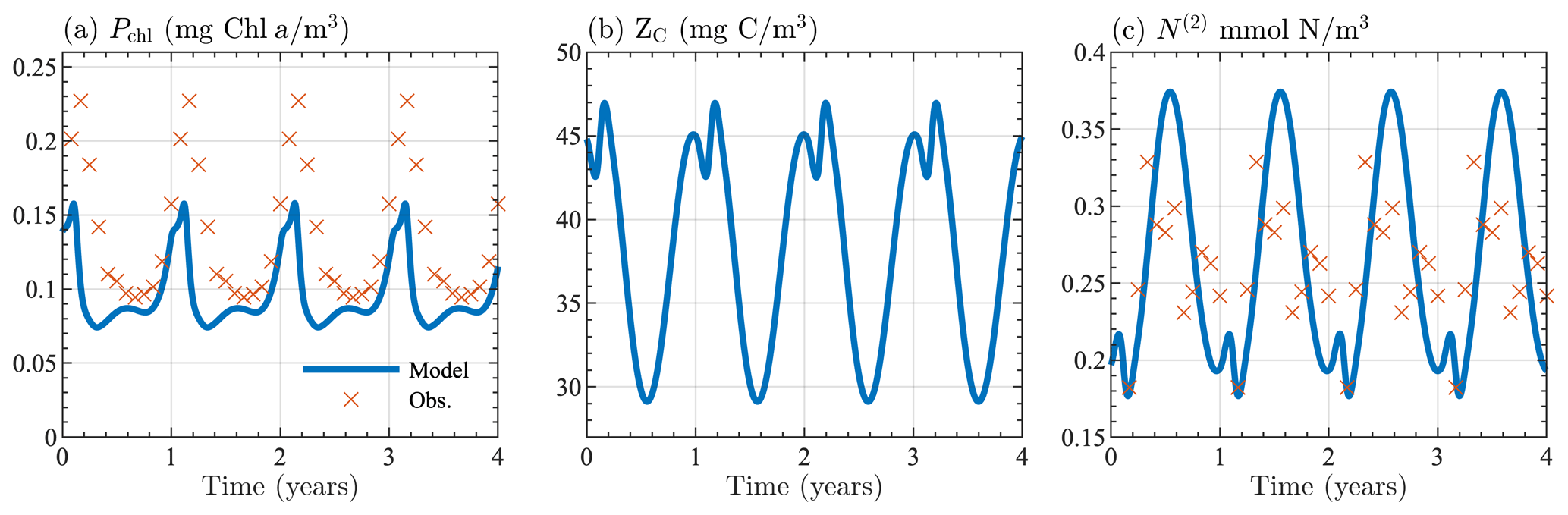
Figure B1 Seasonal cycle of surface (a) chlorophyll, (b) zooplankton carbon, and (c) nitrate from the 0-D test of BFM17. Results are shown for the last 4 years of the 10-year simulation. Panels (a) and (c) show monthly averaged values taken from the observational data described in Sect. 4.

Initial values for chlorophyll, oxygen, phosphate, and nitrate were taken to be similar to values from the BATS/BTM observational data, with P_chl=0.2 mg Chl a m⁻³, O=230 mmol O₂ m⁻³, N⁽¹⁾=0.06 mmol P m⁻³, and N⁽²⁾=1.0 mmol N m⁻³). Phytoplankton carbon was calculated using the maximum chlorophyll-to-carbon ratio, ${\mathit{\theta }}_{\mathrm{chl}}^{\left(\mathrm{0}\right)}$ in Table A3. Initial values for zooplankton carbon, dissolved carbon, and particulate organic carbon were assumed to be the same as the phytoplankton carbon. Ammonium was assumed to have the same initial concentration as phosphate. All other constituents were calculated using their respective optimal ratios in Tables A3 and A4.

Figure B1 shows the seasonal cycle of surface chlorophyll, zooplankton carbon, and nitrate over the last 4 years of the 10-year simulation period, indicating that a stable seasonal cycle with reasonable ecosystem values can be attained by the model, regardless of its coupling to a physical model. Figure B1a and c also show monthly averaged values taken from the observational data described in Sect. 4. Although the agreement between the 0-D BFM17 model and the observations is not perfect, both are qualitatively similar and close in magnitude, providing confidence in the accuracy of the model despite the lower fidelity of the 0-D test.