Towards a model for structured mass movements: the OpenLISEM hazard model 2.0a

Mass movements such as debris flows and landslides differ in behaviour due to their material properties and internal forces. Models employ generalized multi-phase flow equations to adaptively describe these complex flow types. Such models commonly assume unstructured and fragmented flow, where internal cohesive strength is insignificant. In this work, existing work on two-phase mass movement equations are extended to include a full stress–strain relationship that allows for runout of (semi-)structured fluid–solid masses. The work provides both the three-dimensional equations and depth-averaged simplifications. The equations are implemented in a hybrid material point method (MPM), which allows for efficient simulation of stress–strain relationships on discrete smooth particles. Using this framework, the developed model is compared to several flume experiments of clay blocks impacting fixed obstacles. Here, both final deposit patterns and fractures compare well to simulations. Additionally, numerical tests are performed to showcase the range of dynamical behaviour produced by the model. Important processes such as fracturing, fragmentation and fluid release are captured by the model. While this provides an important step towards complete mass movement models, several new opportunities arise, such as application to fragmenting mass movements and block slides.

1 Introduction

The Earth's rock cycle involves sudden release and gravity-driven transport of sloping materials. These mass movements have a significant global impact in financial damage and casualties (Nadim et al., 2006; Kjekstad and Highland, 2009). Understanding the physical principles at work at their initiation and runout phase allows for better mitigation and adaptation to the hazard they induce (Corominas et al., 2014). Many varieties of gravitationally driven mass movements have been categorized according to their material physical parameters and type of movement. Examples are slides, flows and falls, consisting of soil, rocks or debris (Varnes, 1987). Major factors in determining the dynamics of mass movement runout are the composition of the moving material and the internal and external forces during initiation and runout.

Within the cluster of existing mass movement processes, a distinction can be made based on the cohesive of the mass during movement. Post-release, a sloping mass might be unstructured, such as mud flows, where grain–grain cohesive strength is absent. Alternatively, the mass can be fragmentative, such as strongly deforming landslides or fragmenting of rock avalanches upon particle impact. Finally, there are coherent or structured mass movements, such as can be the case for block slides where internal cohesive strength can resist deformation for some period (Varnes, 1987). The general importance of the initially structured nature of mass movement material is observed for a variety of reasons. First, block slides are an important subset of mass movement types (Hayir, 2003; Beutner and Gerbi, 2005; Reiche, 1937; Tang et al., 2009). This type of mass movement features some cohesive structure to the dynamic material in the movement phase. Secondly, during movement, the spatial gradients in local acceleration induce strain and stress that results in fracturing. This process, often called fragmentation in relation to structured mass movements, can be of crucial importance for mass movement dynamics (Davies and McSaveney, 2009; Delaney and Evans, 2014; Dufresne et al., 2018; Corominas et al. 2019). The lubricating effect from basal fragmentation can enhance velocities and runout distance significantly (Davies et al., 2006; Tang et al., 2009). Otherwise, fragmentation generally influences the rheology of the movement by altering grain–grain interactions (Zhou et al., 2005). The importance of structured material dynamics is further indicated by engineering studies on rock behaviour and fracture models (Kaklauskas and Ghaboussi, 2001; Ngekpe et al., 2016; Dhanmeher, 2017).

Dynamics of geophysical flows are complex and depend on a variety of forces due to their multi-phase interactions (Hutter et al., 1994). Physically based models attempt to describe the internal and external forces of all of these mass movements in a generalized form (David and Richard, 2011; Pudasaini, 2012; Iverson and George, 2014). This allows these models to be applied to a wide variety of cases, while improving predictive range. A variety of both one-, two- and three-dimensional sets of equations exist to describe the advection and forces that determine the dynamics of geophysical flows.

For unstructured (fully fragmented) mass movements, a variety of models exist relating to Mohr–Coulomb mixture theory. Such mass movements are described as non-Newtonian granular flows with dominant particle–particle interactions, assuming perfect mixing and continuous movement. Examples are debris flows and mudslides, while block slides and rockslides do not fit these criteria. Within these models, the Mohr–Coulomb failure surface is described with zero cohesive strength and only an internal friction angle (Pitman and Le, 2005). Examples that simulated a single mixed material exist throughout the literature (e.g. Rickenmann et al., 2006; Julien and O'Brien, 1997; Luna et al., 2012; van Asch et al., 2014). Two-phase models describe solids, fluids, and their interactions; provide additional detail; and generalize in important ways (Sheridan et al., 2005; Pitman and Le, 2005; Pudasaini, 2012; Iverson and George, 2014; Mergili et al., 2017). Recently, a three-phase model has been developed that includes the interactions between small and larger solid phases (Pudasaini and Mergili, 2019). Typically, implemented forces include gravitational forces and, depending on the rheology of the equations, drag forces, viscous internal forces and a plasticity criterion. The assumption of zero cohesion in the Mohr–Coulomb material is invalid for any structured mass movement. Some models do implement a non-Newtonian viscous yield stress based on depth-averaged strain estimations (Boetticher et al., 2017; Fornes et al., 2017; Pudasaini and Mergili, 2019). However, this approach lacks the process of fragmentation and internal failure.

For structured mass movements, limited approaches are available. These movements feature some discrete inter-particle connectivity that allows the moving material to maintain a elasto-plastic structure. Examples here are block slides, rockslides and some landslides (Aaron and Hungr, 2016). These materials can be described by a Mohr–Coulomb material with cohesive strength (Spencer, 2012). Aaron and Hungr developed a model for simulation of initially coherent rock avalanches (Aaron and Hungr, 2016) as part of DAN3D Flex. Within their approach, a rigid-block momentum analysis is used to simulate initial movement of the block. After a specified time, the block is assumed to fragment, and a granular flow model using a Voellmy-type rheology is used for further runout. Their approach thus lacks a physical basis for the fragmenting behaviour. Additionally, by dissecting the runout process in two stages (discrete block and granular flow), benefits of holistic two-phase generalized runout models are lost. Finally, Greco et al. (2019) presented a runout model for cohesive granular matrix. Their approach similarly lacks a description of the fragmentation process. Thus, within current mass movement models, there might be improvements available from assuming non-fragmented movement. This would allow for description of structured mass movement dynamics.

In this paper, a generalized mass movement model is developed to describe runout of an arbitrarily structured two-phase Mohr–Coulomb material. The model extents on recent innovations in generalized models for Mohr–Coulomb mixture flow (Pudasaini, 2012; Pudasaini and Mergili, 2019). Section 2 provides the derivation of the extensive set of equations that describe structured mass movements in a generalized manner. Section 3 validates the developed model by comparison with results from controlled flume runout experiments. Additionally, Sect. 3 shows numerical simulation examples that highlight fragmentation behaviour and its influence on runout dynamics. Finally, in Sect. 4 a discussion on the potential usage of the presented model is provided, together with reflection on important opportunities of improvement.

2 A set of mass movement equations incorporating internal structure

2.1 Structured mass movements

Gravitational mass flows are triggered when the local driving forces within an often steep section of a slope exceed a critical threshold. The instability of such materials is generally understood to take place along a failure plane (Zhang et al., 2011; Stead and Wolter, 2015). Along this plane, forces exerted due to gravity and possible seismic accelerations can act as a driving force towards the downslope direction, while a normal force on the terrain induces a resisting force (Xie et al., 2006). When internal stress exceeds specified criteria, commonly described using Mohr–Coulomb theory, fracturing occurs, and the material becomes dynamic. Observations indicate material can initially fracture predominantly at the failure plane (Tang et al., 2009; Davies et al., 2006). Full finite-element modelling of stability confirms no fragmentation occurs at initiation, and runout can start as a structured mass (Matsui and San, 1992; Griffiths and Lane, 1999).

Once movement is initiated, the material is accelerated. Due to spatially non-homogeneous acceleration, either caused by a non-homogeneous terrain slope or impact with obstacles, internal stress can build within the moving mass. The stress state can reach a point outside the yield surface, after which some form of deformation occurs (e.g. plastic, brittle, ductile) (Loehnert et al., 2008). In the case of rock or soil material, elastic or plastic deformation is limited, and fracturing occurs at relatively low strain values (Kaklauskas and Ghaboussi, 2001; Dhanmeher, 2017). Rocks and soil additionally show predominantly brittle fracturing, where strain increments at maximum stress are small (Bieniawaski, 1967; Price, 2016; Hušek et al., 2016). For soil matrices, cohesive bonds between grains originate from causes such as cementing, frictional contacts and root networks (Cohen et al., 2009). Thus, the material breaks along either the grain–grain bonds or on the molecular level. In practice, this process of fragmentation has frequently been both observed and studied. Cracking models for solids use stress–strain descriptions of continuum mechanics (Menin et al., 2009; Ngekpe et al., 2016). Fracture models frequently use smooth particle hydrodynamics (SPH) since a Lagrangian, mesh-free solution benefits possible fracturing behaviour (Maurel and Combescure, 2008; Xu et al., 2010; Osorno and Steeb, 2017). Within the model developed below, knowledge from fracture-simulating continuum mechanical models is combined with finite-element fluid dynamic models.

The Mohr–Coulomb mixture models on which the developed model is based can be found in Pitman and Le (2005), Pudasaini (2012), Iverson and George, (2014), and Pudasaini and Mergili (2019). While these are commonly named debris flow models, their validity extends beyond this typical category of mass movement. This is both apparent from model applications (Mergili et al., 2018) and theoretical considerations (Pudasaini, 2012). A major cause for the usage of debris flow as a term here is the assumption of unstructured flow, which we are aiming to solve in this work.

2.2 Model description

We define two phases within the flow, solids and fluids, indicated by s and f, respectively. A specified fraction of solids within this mixture is at any point part of a structured matrix. This structured solid phase, indicated by sc, envelops and confines a fraction of the fluids in the mixture, indicated by fc. The solids and fluids are defined in terms of the physical properties such as densities (ρ_f,ρ_s) and volume fractions (${\mathit{\alpha }}_{\mathrm{f}}=\frac{f}{f+s},{\mathit{\alpha }}_{\mathrm{s}}=\frac{s}{f+s})$. The confined fractions of their respective phases are indicated as f_sc and f_fc for the volume fraction of confined solids and fluids, respectively (Eqs. 1, 2 and 3).

$$\begin{array}{}\text{(1)}& {\displaystyle }{\mathit{\alpha }}_{\mathrm{s}}+{\mathit{\alpha }}_{\mathrm{f}}=\mathrm{1}\text{(2)}& {\displaystyle }{\mathit{\alpha }}_{\mathrm{s}}\left(f_{\mathrm{sc}}+\left(\mathrm{1}-f_{\mathrm{sc}}\right)\right)+{\mathit{\alpha }}_{\mathrm{f}}\left(f_{\mathrm{fc}}+\left(\mathrm{1}-f_{\mathrm{fc}}\right)\right)=\mathrm{1}\text{(3)}& {\displaystyle }\left(f_{\mathrm{sc}}+\left(\mathrm{1}-f_{\mathrm{sc}}\right)\right)=\left(f_{\mathrm{fc}}+\left(\mathrm{1}-f_{\mathrm{fc}}\right)\right)=\mathrm{1}\end{array}$$

For the solids, internal friction angle (ϕ_s) and effective (volume-averaged) material size (d_s) are additionally defined. We also define ${\mathit{\alpha }}_{\mathrm{c}}={\mathit{\alpha }}_{\mathrm{s}}+f_{\mathrm{fc}}{\mathit{\alpha }}_{\mathrm{f}}$ and ${\mathit{\alpha }}_{\mathrm{u}}=(\mathrm{1}-f_{\mathrm{fc}}){\mathit{\alpha }}_{\mathrm{f}}$ to indicate the solids with confined-fluid and free-fluid phases, respectively. These phases have a volume-averaged density ρ_sc,ρ_f. We let the velocities of the unconfined fluid phase (${\mathit{\alpha }}_{\mathrm{u}}=(\mathrm{1}-f_{\mathrm{fc}}){\mathit{\alpha }}_{\mathrm{f}}$) be defined as $u_{\mathrm{u}}=\left(u_{\mathrm{u}},v_{\mathrm{u}}\right)$. We assume velocities of the confined phases (${\mathit{\alpha }}_{\mathrm{c}}={\mathit{\alpha }}_{\mathrm{s}}+f_{\mathrm{fc}}{\mathit{\alpha }}_{\mathrm{f}}$) can validly be assumed to be identical to the velocities of the solid phase, $u_{\mathrm{c}}=\left(u_{\mathrm{c}},v_{\mathrm{c}}\right)=u_{\mathrm{s}}=\left(u_{\mathrm{s}},v_{\mathrm{s}}\right)$. A schematic depiction of the represented phases is shown in Fig. 1.

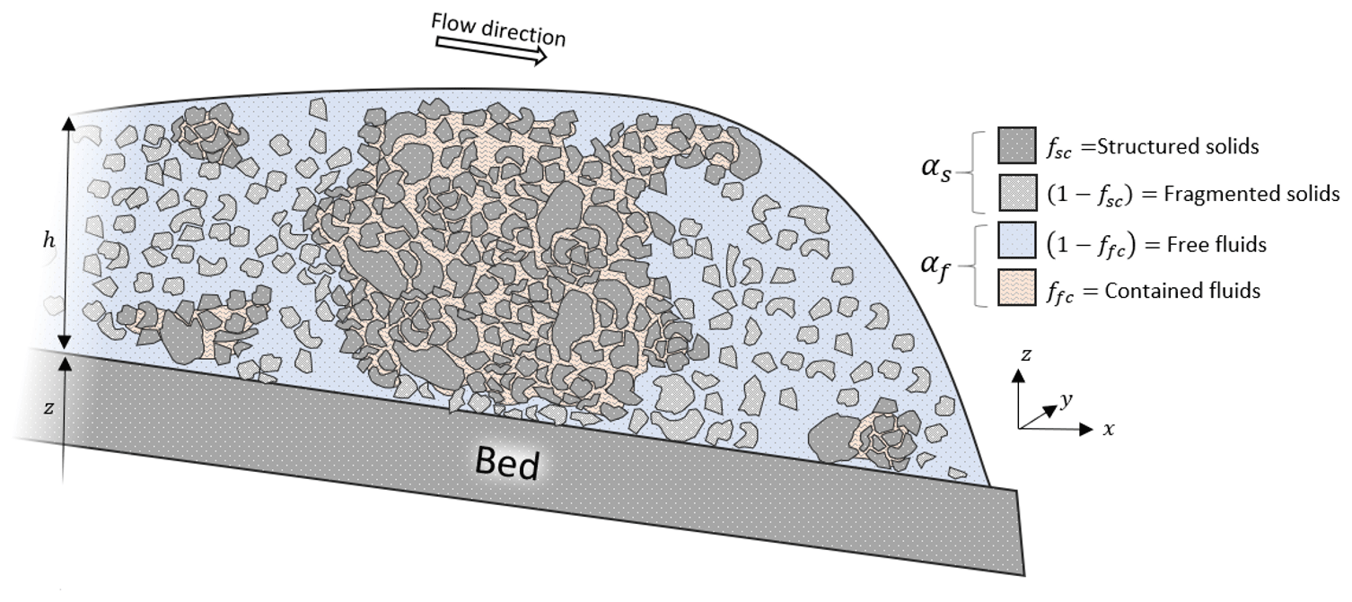
Figure 1 A schematic depiction of the flow contents. Both structured and unstructured solids are present. Fluids can be either free or confined by the structured solids.

A major assumption is made here concerning the velocities of both the confined and free solids (sc and s), that have a shared averaged velocity (u_s). We deliberately limit the flow description to two phases, opposed to the innovative work of Pudasaini and Mergili (2019) that develop a multi-mechanical three-phase model. This choice is motivated by considerations of applicability (reducing the number of required parameters), the infancy of three-phase flow descriptions and finally the general observations of the validity of this assumption (Ishii, 1975; Ishii and Zuber, 1979; Drew, 1983; Jakob et al., 2005; George and Iverson, 2016).

The movement of the flow is described initially by means of mass and momentum conservation (Eqs. 4 and 5).

$$\begin{array}{}\text{(4)}& {\displaystyle \frac{\partial {\mathit{\alpha }}_{\mathrm{c}}}{\partial t}}+\mathrm{\nabla }\cdot \left({\mathit{\alpha }}_{\mathrm{c}}{\mathit{u}}_{\mathrm{c}}\right)=\mathrm{0}\text{(5)}& {\displaystyle \frac{\partial {\mathit{\alpha }}_{\mathrm{u}}}{\partial t}}+\mathrm{\nabla }\cdot \left({\mathit{\alpha }}_{\mathrm{u}}{\mathit{u}}_{\mathrm{u}}\right)=\mathrm{0}\end{array}$$

Here we add the individual forces based on the work of Pudasaini and Hutter (2003), Pitman and Le (2005), Pudasaini (2012), Pudasaini and Fischer (2016), and Pudasaini and Mergili (2019) (Eqs. 6 and 7).

$$\begin{array}{}\text{(6)}& {\displaystyle }\begin{array}{rl}{\displaystyle \frac{\partial }{\partial t}}\left({\mathit{\alpha }}_{\mathrm{c}}{\mathit{\rho }}_{\mathrm{c}}{\mathbf{u}}_{\mathrm{c}}\right)+\mathrm{\nabla }\cdot \left({\mathit{\alpha }}_{\mathrm{c}}{\mathit{\rho }}_{\mathrm{c}}{\mathbf{u}}_{\mathrm{c}}\otimes {\mathbf{u}}_{\mathrm{c}}\right)& ={\mathit{\alpha }}_{\mathrm{c}}{\mathit{\rho }}_{\mathrm{c}}\mathbf{f}\\ & -\mathrm{\nabla }\cdot {\mathit{\alpha }}_{\mathrm{c}}{\mathbf{T}}_{\mathrm{c}}+p_{\mathrm{c}}\mathrm{\nabla }{\mathit{\alpha }}_{\mathrm{c}}\\ & +{\mathbf{M}}_{\mathrm{DG}}+{\mathbf{M}}_{\mathrm{vm}}\end{array}\text{(7)}& {\displaystyle }\begin{array}{rl}{\displaystyle \frac{\partial }{\partial t}}\left({\mathit{\alpha }}_{\mathrm{u}}{\mathit{\rho }}_{\mathrm{f}}{\mathbf{u}}_{\mathrm{u}}\right)+\mathrm{\nabla }\cdot \left({\mathit{\alpha }}_{\mathrm{u}}{\mathit{\rho }}_{\mathrm{f}}{\mathbf{u}}_{\mathrm{u}}\otimes {\mathbf{u}}_{\mathrm{u}}\right)& ={\mathit{\alpha }}_{\mathrm{u}}{\mathit{\rho }}_{\mathrm{f}}\mathbf{f}\\ & -\mathrm{\nabla }\cdot {\mathit{\alpha }}_{\mathrm{u}}{\mathbf{T}}_u+p_{\mathrm{f}}\mathrm{\nabla }{\mathit{\alpha }}_{\mathrm{u}}\\ & -{\mathbf{M}}_{\mathrm{DG}}-{\mathbf{M}}_{\mathrm{vm}}\end{array}\end{array}$$

Here f is the body force (a part of which is gravity), M_DG is the drag force, M_vm is the virtual mass force, and T_candT_u are the stress tensors for solids with confined fluids and unconfined phases, respectively. The virtual mass force described the additional work required by differential acceleration of the phases. The drag force describes the drag along the interfacial boundary of fluids and solids. The body force describes external forces such as gravitational acceleration and boundary forces. Finally, the stress tensors describe the internal forces arising from strain and viscous processes. Both the confined and unconfined phases in the mixture are subject to stress tensors (T_c, and T_u), for which the gradient acts as a momentum source. Additionally, we follow Pudasaini (2012) and add a buoyancy force (p_c∇α_c and p_f∇α_u).

2.2.1 Stress tensors describing internal structure

Based on known two-phase mixture theory, the internal and external forces acting on the moving material are now set up. This results in several unknowns, such as the stress tensors (T_c and T_u, described by the constitutive equation), the body force (f), the drag force (M_DG) and the virtual mass force (M_vm). This section will first describe the derivation of the stress tensors. These describe the internal stress and viscous effects. To describe structured movements, these require a full stress–strain relationship, which is not present in earlier generalized mass movements models. Afterwards, existing derivation of the body, drag and virtual mass force are altered to conform the new constitutive equation.

Our first step in defining the momentum source terms in Eqs. (6) and (7) is the definition of the fluid and solid stress tensors. Current models typically follow the assumptions made by Pitman and Le (2005), who indicate that “the proportionality (and alignment) of the tangential and normal forces that is imposed as a basal boundary condition is assumed to hold throughout the thin flowing layer of material … following Rankine (1857), an earth–pressure relation is assumed for diagonal stress components.” Here, the earth–pressure relationship is a vertically averaged analytical solution for lateral forces exerted by an earth wall. Thus, unstructured columns of moving mixtures are assumed. Here, we aim to use the full Mohr–Coulomb relations. Describing the internal stress of soil and rock matrices is commonly achieved by elasto-plastic simulations of the material's stress–strain relationship. Since we aim to model a full stress description, the stress tensor is equal to the elasto-plastic stress tensor (Eq. 8).

$$\begin{array}{}\text{(8)}& {\mathbf{T}}_{\mathrm{c}}=\mathit{\sigma }\end{array}$$

Here σ is the elasto-plastic stress tensor for solids. The stress can be divided into the deviatoric and non-deviatoric contributions (Eq. 9). The non-deviatoric part acts normally on any plane element (in the manner in which a hydrostatic pressure acts equally in all directions). Note that we switch to tensor notation when describing the stress–strain relationship. Thus, superscripts (α and β) represent the indices of basis vectors (x, y, or z axis in Euclidian space), and obtain tensor elements. Additionally, the Einstein convention is followed (automatic summation of non-defined repeated indices in a single term).

$$\begin{array}{}\text{(9)}& {\mathit{\sigma }}^{\mathit{\alpha }\mathit{\beta }}=s^{\mathit{\alpha }\mathit{\beta }}+{\displaystyle \frac{\mathrm{1}}{\mathrm{3}}}{\mathit{\sigma }}^{\mathit{\gamma }\mathit{\gamma }}{\mathit{\delta }}^{\mathit{\alpha }\mathit{\beta }}\end{array}$$

Here s is the deviatoric stress tensor and ${\mathit{\delta }}^{\mathit{\alpha }\mathit{\beta }}=[\mathit{\alpha }=\mathit{\beta }]$ is the Kronecker delta.

Here, we define the elasto-plastic stress (σ) based on a generalized Hooke-type law in tensor notation (Eqs. 10 and 11), where plastic strain occurs when the stress state reaches the yield criterion (Spencer, 2012; Necas, and Hlavácek, 2017; Bui et al., 2008).

$$\begin{array}{}\text{(10)}& {\displaystyle }{\dot{\mathit{ϵ}}}_{\mathrm{elastic}}^{\mathit{\alpha }\mathit{\beta }}={\displaystyle \frac{{\dot{s}}^{\mathit{\alpha }\mathit{\beta }}}{\mathrm{2}G}}+{\displaystyle \frac{\mathrm{1}-\mathrm{2}\mathit{\nu }}{E}}{\dot{\mathit{\sigma }}}^{\mathrm{m}}{\mathit{\delta }}^{\mathit{\alpha }\mathit{\beta }}\text{(11)}& {\displaystyle }{\dot{\mathit{ϵ}}}_{\mathrm{plastic}}^{\mathit{\alpha }\mathit{\beta }}=\dot{\mathit{\lambda }}{\displaystyle \frac{\partial g}{\partial {\mathit{\sigma }}^{\mathit{\alpha }\mathit{\beta }}}}\end{array}$$

Here ${\dot{\mathit{ϵ}}}_{\mathrm{elastic}}$ is the elastic strain tensor, ${\dot{\mathit{ϵ}}}_{\mathrm{plastic}}$ is the plastic strain tensor, ${\dot{\mathit{\sigma }}}^{\mathrm{m}}$ is the mean stress rate tensor, ν is Poisson's ratio, E is the elastic Young's modulus, G is the shear modulus, $\dot{s}$ is the deviatoric shear stress rate tensor, $\dot{\mathit{\lambda }}$ is the plastic multiplier rate and g is the plastic potential function. Additionally, the strain rate is defined from velocity gradients as Eq. (12).

$$\begin{array}{}\text{(12)}& {\dot{\mathit{ϵ}}}_{\mathrm{total}}^{\mathit{\alpha }\mathit{\beta }}={\dot{\mathit{ϵ}}}_{\mathrm{elastic}}^{\mathit{\alpha }\mathit{\beta }}+{\dot{\mathit{ϵ}}}_{\mathrm{plastic}}^{\mathit{\alpha }\mathit{\beta }}={\displaystyle \frac{\mathrm{1}}{\mathrm{2}}}\left({\displaystyle \frac{\partial u_{\mathrm{c}}^{\mathit{\alpha }}}{\partial x^{\mathit{\beta }}}}-{\displaystyle \frac{\partial u_{\mathrm{c}}^{\mathit{\beta }}}{\partial x^{\mathit{\alpha }}}}\right)\end{array}$$

By solving Eqs. (9), (10) and (11) for $\dot{\mathit{\sigma }}$, a stress–strain relationship can be obtained (Eq. 13) (Bui et al., 2008).

$$\begin{array}{}\text{(13)}& \begin{array}{rl}{\dot{\mathit{\sigma }}}^{\mathit{\alpha }\mathit{\beta }}& =\mathrm{2}G{\dot{e}}^{\mathit{\gamma }\mathit{\gamma }}{\mathit{\delta }}^{\mathit{\alpha }\mathit{\beta }}+K{\dot{\mathit{ϵ}}}^{\mathit{\gamma }\mathit{\gamma }}{\mathit{\delta }}^{\mathit{\alpha }\mathit{\beta }}-\dot{\mathit{\lambda }}\\ & \left[\left(K-{\displaystyle \frac{\mathrm{2}G}{\mathrm{3}}}\right){\displaystyle \frac{\partial g}{\partial {\mathit{\sigma }}^{\mathrm{mn}}}}{\mathit{\delta }}^{\mathrm{mn}}{\mathit{\delta }}^{\mathit{\alpha }\mathit{\beta }}+\mathrm{2}G{\displaystyle \frac{\partial g}{\partial {\mathit{\sigma }}^{\mathit{\alpha }\mathit{\beta }}}}\right]\end{array}\end{array}$$

Here $\dot{e}$ is the deviatoric strain rate (${\dot{e}}^{\mathit{\alpha }\mathit{\beta }}={\dot{\mathit{ϵ}}}^{\mathit{\gamma }\mathit{\gamma }}-\frac{\mathrm{1}}{\mathrm{3}}{\dot{\mathit{ϵ}}}^{\mathit{\alpha }\mathit{\beta }}{\mathit{\delta }}^{\mathit{\alpha }\mathit{\beta }}$), ψ is the dilatancy angle, and K is the elastic bulk modulus and the material parameters defined from E and ν (Eq. 14).

$$\begin{array}{}\text{(14)}& K={\displaystyle \frac{E}{\mathrm{3}(\mathrm{1}-\mathrm{2}\mathit{\nu })}},G={\displaystyle \frac{E}{\mathrm{2}(\mathrm{1}+\mathit{\nu })}}\end{array}$$

Fracturing or failure occurs when the stress state reaches the yield surface, after which plastic deformation occurs. The rate of change of the plastic multiplier specifies the magnitude of plastic loading and must ensure a new stress state conforms to the conditions of the yield criterion. By means of substituting Eq. (13) in the consistency condition ($\frac{\partial f}{\partial {\mathit{\sigma }}^{\mathit{\alpha }\mathit{\beta }}}d{\mathit{\sigma }}^{\mathit{\alpha }\mathit{\beta }}=\mathrm{0}$), the plastic multiplier rate can be defined (Eq. 15) (Bui et al., 2008).

$$\begin{array}{}\text{(15)}& \dot{\mathit{\lambda }}={\displaystyle \frac{\mathrm{2}G{\mathit{ϵ}}^{\mathit{\alpha }\mathit{\beta }}\frac{\partial f}{\partial {\mathit{\sigma }}^{\mathit{\alpha }\mathit{\beta }}}+\left(K-\frac{\mathrm{2}G}{\mathrm{3}}\right){\dot{\mathit{ϵ}}}^{\mathit{\gamma }\mathit{\gamma }}\frac{\partial f}{\partial {\mathit{\sigma }}^{\mathit{\alpha }\mathit{\beta }}}{\mathit{\sigma }}^{\mathit{\alpha }\mathit{\beta }}{\mathit{\delta }}^{\mathit{\alpha }\mathit{\beta }}}{\mathrm{2}G\frac{\partial f}{\partial {\mathit{\sigma }}^{\mathrm{mn}}}\frac{\partial g}{\partial {\mathit{\sigma }}^{\mathrm{mn}}}+\left(K-\frac{\mathrm{2}G}{\mathrm{3}}\right)\frac{\partial f}{\partial {\mathit{\sigma }}^{\mathrm{mn}}}{\mathit{\delta }}^{\mathrm{mn}}\frac{\partial g}{\partial {\mathit{\sigma }}^{\mathrm{mn}}}{\mathit{\delta }}^{\mathrm{mn}}}}\end{array}$$

The yield criteria specifies a surface in the stress state space that the stress state can not pass and at which plastic deformation occurs. A variety of yield criteria exist, such as Mohr–Coulomb, Von Mises, Drucker–Prager and Tresca (Spencer, 2012). Here, we employ the Drucker–Prager model fitted to Mohr–Coulomb material parameters for its accuracy in simulating rock and soil behaviour and numerical stability (Spencer, 2012; Bui et al., 2008) (Eqs. 16 and 17).

$$\begin{array}{}\text{(16)}& {\displaystyle }f\left(I_{\mathrm{1}},J_{\mathrm{2}}\right)=\sqrt{J_{\mathrm{2}}}+{\mathit{\alpha }}_{\mathit{\varphi }}{I}_{\mathrm{1}}-k_{\mathrm{c}}=\mathrm{0}\text{(17)}& {\displaystyle }g\left(I_{\mathrm{1}},J_{\mathrm{2}}\right)=\sqrt{J_{\mathrm{2}}}+{\mathit{\alpha }}_{\mathit{\varphi }}{I}_{\mathrm{1}}\sin \left(\mathit{\psi }\right)\end{array}$$

Here I₁ and J₂ are tensor invariants (Eqs. 18 and 19).

$$\begin{array}{}\text{(18)}& {\displaystyle }{I}_{\mathrm{1}}={\mathit{\sigma }}^{xx}+{\mathit{\sigma }}^{yy}+{\mathit{\sigma }}^{zz}\text{(19)}& {\displaystyle }{J}_{\mathrm{2}}={\displaystyle \frac{\mathrm{1}}{\mathrm{2}}}{s}^{\mathit{\alpha }\mathit{\beta }}{s}^{\mathit{\alpha }\mathit{\beta }}\end{array}$$

Here the Mohr–Coulomb material parameters are used to estimate the Drucker–Prager parameters (Eq. 20).

$$\begin{array}{}\text{(20)}& {\mathit{\alpha }}_{\mathit{\varphi }}={\displaystyle \frac{\tan \left(\mathit{\varphi }\right)}{\sqrt{\mathrm{9}+\mathrm{12}{\tan }^{\mathrm{2}}\mathit{\varphi }}}},k_{\mathrm{c}}={\displaystyle \frac{\mathrm{3}c}{\sqrt{\mathrm{9}+\mathrm{12}{\tan }^{\mathrm{2}}\mathit{\varphi }}}}\end{array}$$

Using the definitions of the yield surface and stress–strain relationship, combining Eqs. (13), (15), (16) and (17), the relationship for the stress rate can be obtained (Eqs. 21 and 22).

$$\begin{array}{}\text{(21)}& {\displaystyle }\dot{\mathit{\sigma }}=\mathrm{2}G{\dot{e}}^{\mathit{\alpha }\mathit{\beta }}+K{\dot{\mathit{ϵ}}}^{\mathit{\gamma }\mathit{\gamma }}{\mathit{\delta }}^{\mathit{\alpha }\mathit{\beta }}-\dot{\mathit{\lambda }}\left[\mathrm{9}K\sin \mathit{\psi }{\mathit{\delta }}^{\mathit{\alpha }\mathit{\beta }}+{\displaystyle \frac{G}{\sqrt{J_{\mathrm{2}}}}}{s}^{\mathit{\alpha }\mathit{\beta }}\right]\text{(22)}& {\displaystyle }\dot{\mathit{\lambda }}={\displaystyle \frac{\mathrm{3}\mathit{\alpha }K{\dot{\mathit{ϵ}}}^{\mathit{\gamma }\mathit{\gamma }}+\left(\frac{G}{\sqrt{J_{\mathrm{2}}}}\right)s^{\mathit{\alpha }\mathit{\beta }}{\dot{\mathit{ϵ}}}^{\mathit{\alpha }\mathit{\beta }}}{\mathrm{27}{\mathit{\alpha }}_{\mathit{\varphi }}K\sin \mathit{\psi }+G}}\end{array}$$

In order to allow for the description of large deformation, the Jaumann stress rate can be used, which is a stress-rate that is independent from a frame of reference (Eq. 23).

$$\begin{array}{}\text{(23)}& \begin{array}{rl}\dot{\widehat{\mathit{\sigma }}}& ={\mathit{\sigma }}^{\mathit{\alpha }\mathit{\gamma }}{\dot{\mathit{\omega }}}^{\mathit{\beta }\mathit{\gamma }}+{\mathit{\sigma }}^{\mathit{\gamma }\mathit{\beta }}{\dot{\mathit{\omega }}}^{\mathit{\alpha }\mathit{\gamma }}+\mathrm{2}G{\dot{e}}^{\mathit{\alpha }\mathit{\beta }}\\ & +K{\dot{\mathit{ϵ}}}^{\mathit{\gamma }\mathit{\gamma }}{\mathit{\delta }}^{\mathit{\alpha }\mathit{\beta }}-\dot{\mathit{\lambda }}\left[\mathrm{9}K\sin \mathit{\psi }{\mathit{\delta }}^{\mathit{\alpha }\mathit{\beta }}+{\displaystyle \frac{G}{\sqrt{J_{\mathrm{2}}}}}{s}^{\mathit{\alpha }\mathit{\beta }}\right]\end{array}\end{array}$$

Here $\dot{\mathit{\omega }}$ is the spin rate tensor, as defined by Eq. (24).

$$\begin{array}{}\text{(24)}& {\dot{\mathit{\omega }}}^{\mathit{\alpha }\mathit{\beta }}={\displaystyle \frac{\mathrm{1}}{\mathrm{2}}}\left({\displaystyle \frac{\partial v^{\mathit{\alpha }}}{\partial x^{\mathit{\beta }}}}-{\displaystyle \frac{\partial v^{\mathit{\beta }}}{\partial x^{\mathit{\alpha }}}}\right)\end{array}$$

Due to the strain within the confined material, the density of the confined solid phase (ρ_c) evolves dynamically according to Eq. (25).

$$\begin{array}{}\text{(25)}& {\mathit{\rho }}_{\mathrm{c}}=f_{\mathrm{sc}}{\mathit{\rho }}_{\mathrm{s}}{\displaystyle \frac{{\mathit{ϵ}}_{\mathrm{v}\mathrm{0}}}{{\mathit{ϵ}}_{\mathrm{v}}}}+\left(\mathrm{1}-f_{\mathrm{sc}}\right){\mathit{\rho }}_{\mathrm{s}}+f_{\mathrm{fc}}{\mathit{\rho }}_{\mathrm{f}}\end{array}$$

Here ϵ_v is the total volume strain, ${\dot{\mathit{ϵ}}}_{\mathrm{v}}\approx {\mathit{ϵ}}_{\mathrm{1}}+{\mathit{ϵ}}_{\mathrm{2}}+{\mathit{ϵ}}_{\mathrm{3}}$, ϵ_i is one of the principal components of the strain tensor. Since we aim to simulate brittle materials, where volume strain remains relatively low, we assume that changes in density are small compared to the original density of the material ($\frac{\partial {\mathit{\rho }}_{\mathrm{c}}}{\partial t}\ll {\mathit{\rho }}_{\mathrm{c}}$).

2.2.2 Fragmentation

Brittle fracturing is a processes commonly understood to take place once a material internal stress has reached the yield surface, and plastic deformation has been sufficient to pass the ultimate strength point (Maurel and Cumescure, 2008; Hušek et al., 2016). A variety of approaches to fracturing exist within the literature (Ma et al., 2014; Osomo and Steeb, 2017). Finite element method (FEM) models use strain-based approaches (Loehnert et al., 2008). For SPH implementations, as will be presented in this work, distance-based approaches have provided good results (Maurel and Cumbescure, 2008). Other works have used strain-based fracture criteria (Xu et al., 2010) . Additionally, dynamic degradation of strength parameters have been implemented (Grady and Kipp, 1980; De Vuyst and Vignjevic, 2013; Williams, 2019). Comparisons with observed fracture behaviour has indicated the predictive value of these schemes (Xu et al., 2010; Hušek et al., 2016). We combine the various approaches to best fit the dynamical multi-phase mass movement model that is developed. Following Grady and Kipp (1980), we simulate a degradation of strength parameters. Our material consists of a soil and rock matrix. We assume fracturing occurs along the inter-granular or inter-rock contacts and bonds (see also Cohen et al., 2009). Thus, cohesive strength is lost for any fractured contacts. We simulate degradation of cohesive strength according to a volume strain criteria. When the stress state lies on the yield surface (the set of critical stress states within the six-dimensional stress-space), during plastic deformation, strain is assumed to contribute to the fracturing of the granular or rock material. A critical volume strain is taken as a material property, and the breaking of cohesive bonds occurs based on the relative volume strain. Following Grady and Kipp (1980) and De Vuyst and Vignjevic (2013), we assume that the degradation behaviour of the strength parameter is distributed according to a probability density distribution. Commonly, a Weibull distribution is used (Williams, 2019). Here, for simplicity we use a uniform distribution of cohesive strength between 0 and 2c₀, although any other distribution can be substituted. Thus, the expression governing cohesive strength becomes Eq. (26).

$$\begin{array}{}\text{(26)}& {\displaystyle \frac{\partial c}{\partial t}}=\left\{\begin{array}{ll}-c_{\mathrm{0}}\frac{\mathrm{1}}{\mathrm{2}}\frac{\left(\frac{{\mathit{ϵ}}_{\mathrm{v}}}{{\mathit{ϵ}}_{\mathrm{v}\mathrm{0}}}\right)}{{\mathit{ϵ}}_{\mathrm{c}}}& f\left(I_{\mathrm{1}},J_{\mathrm{2}}\right)\ge \mathrm{0},c>\mathrm{0}\\ \mathrm{0}& \mathrm{otherwise}\end{array}\right.\end{array}$$

Here c₀ is the initial cohesive strength of the material, ϵ_v0 is the initial volume, $\left(\frac{{\mathit{ϵ}}_{\mathrm{v}}}{{\mathit{ϵ}}_{\mathrm{v}\mathrm{0}}}\right)$ is the fractional volumetric strain rate and ϵ_c is the critical fractional volume strain for fracturing.

2.2.3 Water partitioning

During the movement of the mixed mass, the solids can thus be present as a structured matrix. Within such a matrix, a fluid volume can be contained (e.g. as originating from a groundwater content in the original landslide material). These fluids are typically described as groundwater flow following Darcy's law, which poses a linear relationship between pressure gradients and flow velocity through a soil matrix. In our case, we assumed the relative velocity of water flow within the granular solid matrix as very small compared to both solid velocities and the velocities of the free fluids. As an initial condition of the material, some fraction of the water is contained within the soil matrix (f_fc). Additionally, for loss of cohesive structure within the solid phase, we transfer the related fraction of fluids contained within that solid structure to the free fluids.

$$\begin{array}{}\text{(27)}& {\displaystyle }\begin{array}{rl}{\displaystyle \frac{\partial f_{\mathrm{fc}}}{\partial t}}& =-{\displaystyle \frac{\partial \left(\mathrm{1}-f_{\mathrm{fc}}\right)}{\partial t}}\\ & =\left\{\begin{array}{ll}-f_{\mathrm{fc}}\frac{c_{\mathrm{0}}}{c}\frac{\max (\mathrm{0.0},{\dot{\mathit{ϵ}}}_{\mathrm{v}})}{{\mathit{ϵ}}_{\mathrm{f}}}& f\left(I_{\mathrm{1}},J_{\mathrm{2}}\right)\ge \mathrm{0},c>\mathrm{0}\\ \mathrm{0}& \mathrm{otherwise}\end{array}\right.\end{array}\text{(28)}& {\displaystyle }\begin{array}{rl}{\displaystyle \frac{\partial f_{\mathrm{sc}}}{\partial t}}& =-{\displaystyle \frac{\partial \left(\mathrm{1}-f_{\mathrm{sc}}\right)}{\partial t}}\\ & =\left\{\begin{array}{ll}-f_{\mathrm{sc}}\frac{c_{\mathrm{0}}}{c}\frac{\max (\mathrm{0.0},{\dot{\mathit{ϵ}}}_{\mathrm{v}})}{{\mathit{ϵ}}_{\mathrm{f}}}& f\left(I_{\mathrm{1}},J_{\mathrm{2}}\right)\ge \mathrm{0},c>\mathrm{0}\\ \mathrm{0}& \mathrm{otherwise}\end{array}\right.\end{array}\end{array}$$

Beyond changes in f_fc through fracturing of structured solid materials, no dynamics are simulated for influx or outflux of fluids from the solid matrix. The initial volume fraction of fluids in the solid matrix defined by ff_fc and sf_sc remains constant throughout the simulation. The validity of this assumption can be based on the slow typical fluid velocities in a solid matrix relative to fragmented mixed fluid–solid flow velocities (Kern, 1995; Saxton and Rawls, 2006). While the addition of evolving saturation would extend the validity of the model, it would require implementation of pre-transfer functions for evolving material properties, which is beyond the scope of this work. An important note on the points made above is the manner in which fluids are re-partitioned after fragmentation. All fluids in fragmented solids are released, but this does not equate to free movement of the fluids or a disconnection from the solids that confined them. Instead, the equations continue to connect the solids and fluids through drag, viscous and virtual mass forces. Finally, the density of the fragmented solids is assumed to be the initially set solid density. Any strain-induced density changes are assumed small relative to the initial solid density ($\frac{{\mathit{\rho }}_{\mathrm{c}}}{{\mathit{\rho }}_{\mathrm{s}}}\ll \mathrm{1}$).

2.2.4 Fluid stresses

The fluid stress tensor is determined by the pressure and the viscous terms (Eqs. 29 and 30). Confined solids are assumed to be saturated and constant during the flow.

$$\begin{array}{}\text{(29)}& {\displaystyle }{\mathbf{T}}_u=p_{\mathrm{f}}\mathbf{I}+{\mathit{\tau }}_{\mathrm{f}}\text{(30)}& {\displaystyle }\begin{array}{rl}{\mathit{\tau }}_{\mathrm{f}}& ={\mathit{\eta }}_{\mathrm{f}}\left[\mathrm{\nabla }{\mathbf{u}}_{\mathrm{u}}+{\left(\mathrm{\nabla }{\mathbf{u}}_{\mathrm{c}}\right)}^t\right]\\ & -{\displaystyle \frac{{\mathit{\eta }}_{\mathrm{f}}}{{\mathit{\alpha }}_{\mathrm{u}}}}\mathcal{A}\left({\mathit{\alpha }}_{\mathrm{u}}\right)\left(\mathrm{\nabla }{\mathit{\alpha }}_{\mathrm{c}}\left({\mathbf{u}}_{\mathrm{u}}-{\mathbf{u}}_{\mathrm{c}}\right)+\left({\mathbf{u}}_{\mathrm{c}}-{\mathbf{u}}_{\mathrm{u}}\right)\mathrm{\nabla }{\mathit{\alpha }}_{\mathrm{c}}\right)\end{array}\end{array}$$

Here I is the identity tensor, τ_f is the viscous stress tensor for fluids , p_f is the fluid pressure, η_f is the dynamic viscosity of the fluids and 𝒜 is the mobility of the fluids at the interface with the solids that acts as a phenomenological parameter (Pudasaini, 2012).

The fluid pressure acts only on the free fluids here, as the confined fluids are moved together with the solids. In Eq. (30), the second term is related to the non-Newtonian viscous force induced by gradients in solid concentration. The effect as described by Pudasaini (2012) is induced by a solid concentration gradient. In the case of unconfined fluids and unstructured solids ($f_{\mathrm{sc}}=\mathrm{0},f_{\mathrm{fc}}=\mathrm{0}$); this force is identical to the description in the unstructured equations. Within our flow description, we see no direct reason to eliminate or alter this force with a variation in the fraction of confined fluids or structured solids. We only consider the interface between solids and free fluids as an agent that induces this effect, and therefore the gradient of the gradient of the solids and confined fluids ($\mathrm{\nabla }({\mathit{\alpha }}_{\mathrm{s}}+f_{\mathrm{fc}}{\mathit{\alpha }}_{\mathrm{f}})=\mathrm{\nabla }{\mathit{\alpha }}_{\mathrm{c}}$) is used instead of the total solid phase (∇α_s).

2.2.5 Drag force and virtual mass

Our description of the drag force follows the work of Pudasaini (2012), Pudasaini et al. (2018), where a generalized two-phase drag model is introduced and enhanced. We split their work into a contribution from the fraction of structured solids (f_sc) and unconfined fluids (1−f_fc) (Eq. 31).

$$\begin{array}{}\text{(31)}& \begin{array}{rl}{\mathcal{C}}_{\mathrm{DG}}& ={\displaystyle \frac{f_{\mathrm{sc}}{\mathit{\alpha }}_{\mathrm{c}}{\mathit{\alpha }}_{\mathrm{u}}\left({\mathit{\rho }}_{\mathrm{c}}-{\mathit{\rho }}_{\mathrm{f}}\right)g}{U_{\mathrm{T},\mathrm{c}}\left(\mathcal{G}\left(Re\right)\right)+S_p}}\left({\mathbf{u}}_{\mathrm{u}}-{\mathbf{u}}_{\mathrm{c}}\right){\left|{\mathbf{u}}_{\mathrm{u}}-{\mathbf{u}}_{\mathrm{c}}\right|}^{j-\mathrm{1}}\\ & +{\displaystyle \frac{(\mathrm{1}-f_{\mathrm{sc}}){\mathit{\alpha }}_{\mathrm{c}}{\mathit{\alpha }}_{\mathrm{u}}\left({\mathit{\rho }}_{\mathrm{s}}-{\mathit{\rho }}_{\mathrm{f}}\right)g}{U_{\mathrm{T},\mathrm{uc}}\left(\mathcal{P}\mathcal{F}\left(R{e}_{\mathrm{p}}\right)+\left(\mathrm{1}-\mathcal{P}\right)\mathcal{G}\left(Re\right)\right)+S_p}}\\ & \left({\mathbf{u}}_{\mathrm{u}}-{\mathbf{u}}_{\mathrm{c}}\right){\left|{\mathbf{u}}_{\mathrm{u}}-{\mathbf{u}}_{\mathrm{c}}\right|}^{j-\mathrm{1}}\end{array}\end{array}$$

Here U_T,c is the terminal or settling velocity of the structured solids, U_T,uc is the terminal velocity of the unconfined solids, 𝒫 is a factor that combines solid- and fluid-like contributions to the drag force, 𝒢 is the solid-like drag contribution, ℱ is the fluid-like drag contribution, and S_p is the smoothing function (Eqs. 32 and 34). The exponent j indicates the type of drag: linear (j=0) or quadratic (j=1).

Within the drag, the following functions are defined:

$$\begin{array}{}\text{(32)}& {\displaystyle }F={\displaystyle \frac{\mathit{\gamma }}{\mathrm{180}}}{\left({\displaystyle \frac{{\mathit{\alpha }}_{\mathrm{f}}}{{\mathit{\alpha }}_{\mathrm{s}}}}\right)}^{\mathrm{3}}R{e}_{\mathrm{p}},G={\mathit{\alpha }}_{\mathrm{f}}^{M\left(R{e}_{\mathrm{p}}\right)-\mathrm{1}}.\text{(33)}& {\displaystyle }{S}_p=({\displaystyle \frac{\mathcal{P}}{{\mathit{\alpha }}_{\mathrm{c}}}}+{\displaystyle \frac{\mathrm{1}-\mathcal{P}}{{\mathit{\alpha }}_{\mathrm{u}}}})\mathcal{K},\text{(34)}& {\displaystyle }\mathcal{K}=\left|{\mathit{\alpha }}_{\mathrm{c}}{\mathbf{u}}_{\mathrm{c}}+{\mathit{\alpha }}_{\mathrm{u}}{\mathbf{u}}_{\mathrm{u}}\right|\approx \mathrm{10}\mathrm{m}{\mathrm{s}}^{-\mathrm{1}},\end{array}$$

where M is a parameter that varies between 2.4 and 4.65 based on the Reynolds number (Pitman and Le, 2005). The factor 𝒫 that combines solid- and fluid-like contributions to the drag is dependent on the volumetric solid content in the unconfined and unstructured materials $\left(\mathcal{P}={\left(\frac{{\mathit{\alpha }}_{\mathrm{s}}(\mathrm{1}-f_{\mathrm{sc}})}{{\mathit{\alpha }}_{\mathrm{f}}\left(\mathrm{1}-f_{\mathrm{fc}}\right)}\right)}^{\mathrm{m}}\right)$ with m≈1. Additionally, we assume the factor 𝒫 is zero for drag originating from the structured solids. As stated by Pudasaini and Mergili (2019), “as limiting cases: 𝒫 suitably models solid particles moving through a fluid”. In our model, the drag force acts on the unconfined fluid momentum (u_ucα_f(1−f_fc)). For interactions between unconfined fluids and structured solids, larger blocks of solid structures are moving through fluids that contains solids of smaller size.

Virtual mass is similarly implemented based on the work of Pudasaini (2012) and Pudasaini and Mergili (2019) (Eq. 35). The adapted implementation considers the solids together with confined fluids to move through a free-fluid phase.

$$\begin{array}{}\text{(35)}& \begin{array}{rl}{\mathcal{C}}_{\mathrm{VMG}}& ={\mathit{\alpha }}_{\mathrm{c}}{\mathit{\rho }}_{\mathrm{u}}\left({\displaystyle \frac{\mathrm{1}}{\mathrm{2}}}\left({\displaystyle \frac{\mathrm{1}+\mathrm{2}{\mathit{\alpha }}_{\mathrm{c}}}{{\mathit{\alpha }}_{\mathrm{u}}}}\right)\right)\left(\left({\displaystyle \frac{\partial u_{\mathrm{u}}}{\partial t}}+u_{\mathrm{u}}\cdot \mathrm{\nabla }{u}_{\mathrm{u}}\right)\right.\\ & \left.-\left({\displaystyle \frac{\partial u_{\mathrm{c}}}{\partial t}}+u_{\mathrm{c}}\cdot \mathrm{\nabla }{u}_{\mathrm{c}}\right)\right)\end{array}\end{array}$$

Here $C_{\mathrm{DG}}=\frac{\mathrm{1}}{\mathrm{2}}\left(\frac{\mathrm{1}+\mathrm{2}{\mathit{\alpha }}_{\mathrm{c}}}{{\mathit{\alpha }}_{\mathrm{u}}}\right)$ is the drag coefficient.

2.2.6 Boundary conditions

Finally, following the work of Iverson and Denlinger (2001), Pitman and Le (2005), and Pudasaini (2012), a boundary condition is applied to the surface elements that contact the flow (Eq. 36).

$$\begin{array}{}\text{(36)}& \left|\mathbf{S}\right|=N\tan \left(\mathit{\varphi }\right)\end{array}$$

Here N is the normal pressure on the surface element and S is the shear stress.

2.3 Depth-averaging

The majority of the depth-averaging in this work is analogous to the work of Pitman and Le (2005), Pudasaini (2012), and Pudasini and Mergili (2019). Depth-averaging through integration over the vertical extent of the flow can be done based on several useful and often-used assumptions, e.g. $\frac{\mathrm{1}}{h}{\int }_{\mathrm{0}}^{h}x\mathrm{d}h=\stackrel{\mathrm{‾}}{x}$, for the velocities (u_u and u_c); solid, fluid, and confined fractions (α_f, α_s, f_fc and f_sc); and material properties (ρ_u, ϕ and c). Besides these similarities and an identical derivation of depth-averaged continuity equations, three major differences arise.

• i.

  Fluid pressure. Previous implementations of generalized two-phase debris flow equations have commonly assumed hydrostatic pressure ($\frac{\partial p}{\partial z}=g^z$) (Pitman and Le, 2005; Pudasaini, 2012; Abe and Konagai, 2016). Here we follow this assumption for the fluid pressure at the base and solid pressure for unstructured material (Eqs. 37 and 38).

  $$\begin{array}{}\text{(37)}& {\displaystyle }{P}_{{\mathrm{b}}_{s,u}}=-\left(\mathrm{1}-\mathit{\gamma }\right){\mathit{\alpha }}_{\mathrm{s}}{g}^{z}h\text{(38)}& {\displaystyle }{P}_{{\mathrm{b}}_{\mathrm{u}}}=-g^{z}h\end{array}$$

  Here $\mathit{\gamma }=\frac{{\mathit{\rho }}_{\mathrm{f}}}{{\mathit{\rho }}_{\mathrm{s}}}$ is the density ratio (not to be confused with a tensor index when used in superscript) (–).

  However, larger blocks of structure material can have contact with the basal topography. Due to density differences, larger blocks of solid structures are likely to move along the base (Pailhia and Pouliquen, 2009; Iverson and George, 2014). If these blocks are saturated, water pressure propagates through the solid matrix and hydrostatic pressure is retained. However, in cases of an unsaturated solid matrix that connects to the base, hydrostatic pressure is not present there. We introduce a basal fluid pressure propagation factor $\mathcal{B}({\mathit{\theta }}_{\mathrm{eff}},\stackrel{\mathrm{‾}}{d_{\mathrm{sc}}},\mathrm{\dots })$ that describes the fraction of fluid pressure propagated through a solid matrix (with θ_eff as the effective saturation, and as $\stackrel{\mathrm{‾}}{d_{\mathrm{sc}}}$ the average size of structured solid matrix blocks). This results in a basal pressure equal to Eq. (39).

  $$\begin{array}{}\text{(39)}& \begin{array}{rl}{P}_{{\mathrm{b}}_{\mathrm{c}}}& =-\left(\mathrm{1}-f_{\mathrm{sc}}\right)\left(\mathrm{1}-\mathit{\gamma }\right){\displaystyle \frac{\left(\mathrm{1}-f_{\mathrm{sc}}\right){\mathit{\alpha }}_{\mathrm{s}}}{\left(\mathrm{1}-f_{\mathrm{fc}}\right){\mathit{\alpha }}_{\mathrm{f}}}}{g}^{z}h\\ & -f_{\mathrm{sc}}\left(\mathrm{1}-\mathit{\gamma }\right)\mathcal{B}{\displaystyle \frac{\left(f_{\mathrm{sc}}\right){\mathit{\alpha }}_{\mathrm{s}}}{\left(f_{\mathrm{fc}}\right){\mathit{\alpha }}_{\mathrm{f}}}}{g}^{z}h\end{array}\end{array}$$

  The basal pressure propagation factor (ℬ) should theoretically depend mostly on saturation level, similarly to the pedotransfer function, as a full saturation means perfect propagation of pressure through the mixture, and low saturation equates to minimal pressure propagation (Saxton and Rawls, 2006). Additionally, it should depend on pedotransfer functions and the size distribution of structured solid matrices within the mixture. For low saturation levels, it can be assumed that no fluid pressure is retained. Combined with an assumed soil matrix height being identical to the total mixture height, this results in ℬ=0. Assuming saturation of a structure's solids results in a full propagation of pressures and ℬ=1.

• ii.

  Stress–strain relationship. Depth-averaging the stress–strain relationship in Eqs. (22) and (23) requires a vertical solution for the internal stress. First, we assume any non-normal vertical terms are zero (Eq. 40). Commonly, Rankine's earth pressure coefficients are used to express the lateral earth pressure by assuming vertical stress to be induced by the basal solid pressure (Eqs. 41 and 42) (Pitman and Le, 2005; Pudasaini, 2012; Abe and Konagai, 2016).

  $$\begin{array}{}\text{(40)}& {\displaystyle }{\mathit{\sigma }}^{zx}={\mathit{\sigma }}^{zy}={\mathit{\sigma }}^{yz}={\mathit{\sigma }}^{xz}=\mathrm{0}\text{(41)}& {\displaystyle }\stackrel{\mathrm{‾}}{{\mathit{\sigma }}^{zz}}={\displaystyle \frac{\mathrm{1}}{\mathrm{2}}}{P}_{{\mathrm{b}}_{\mathrm{s}}},{\mathit{\sigma }}^{zz}{}_{\mathrm{b}}=P_{{\mathrm{b}}_{\mathrm{s}}}\text{(42)}& {\displaystyle }{K}_{\mathrm{a}}={\displaystyle \frac{\mathrm{1}-\sin \left(\mathit{\varphi }\right)}{\mathrm{1}+\sin \left(\mathit{\varphi }\right)}},K_{\mathrm{p}}={\displaystyle \frac{\mathrm{1}-\sin \left(\mathit{\varphi }\right)}{\mathrm{1}+\sin \left(\mathit{\varphi }\right)}}\end{array}$$

  Here we enhance this with Bell's extension for cohesive soils (Eq. 45) (Xu et al., 2019). This lateral normal-directed stress term is added to the full stress–strain solution.

  $$\begin{array}{}\text{(43)}& \stackrel{\mathrm{‾}}{{\mathit{\sigma }}_{xx}}=K{\mathit{\sigma }}_{zz}{}_{\mathrm{b}}-\mathrm{2}c\sqrt{K}+{\displaystyle \frac{\mathrm{1}}{h}}{\int }_{\mathrm{0}}^h{\mathit{\sigma }}_{xx}\mathrm{d}h\end{array}$$

  Finally, the gradient in pressure of the lateral interfaces between the mixture is added as a depth-averaged acceleration term (Eq. 44).

  $$\begin{array}{}\text{(44)}& S_{x_{\mathrm{c}}}={\mathit{\alpha }}_{\mathrm{c}}\left({\displaystyle \frac{\mathrm{1}}{h}}\left({\displaystyle \frac{\partial \left(h{\mathit{\sigma }}^{xx}\right)}{\partial x}}+{\displaystyle \frac{\partial \left(h{\mathit{\sigma }}^{yx}\right)}{\partial y}}\right)\right)+\mathrm{\dots }\end{array}$$
• iii.

  Depth-averaging other terms. While the majority of terms allow for depth-averaging as it was proposed by Pudasaini (2012), an exception arises. Depth-averaging of the vertical viscosity terms is required. The non-Newtonian viscous terms for the fluid phase were derived assuming a vertical profile in the volumetric solid phase content. Here, we alter the derivation to use this assumption only for the non-structured solids, as opposed to the structured solids where $\frac{\partial {\mathit{\alpha }}_{\mathrm{s}}}{\partial z}=\mathrm{0}$.

  $$\begin{array}{}\text{(45)}& \begin{array}{rl}{\int }_{\mathrm{b}}^{\mathrm{s}}{\displaystyle \frac{\partial }{\partial z}}\left({\displaystyle \frac{\partial {\mathit{\alpha }}_{\mathrm{s}}}{\partial z}}\left(u_{\mathrm{u}}-u_{\mathrm{c}}\right)\right)\mathrm{d}z& ={\left[{\displaystyle \frac{\partial {\mathit{\alpha }}_{\mathrm{s}}}{\partial z}}\left(u_{\mathrm{u}}-u_{\mathrm{c}}\right)\right]}_{\mathrm{b}}^{\mathrm{s}}\\ & =\left(\stackrel{\mathrm{‾}}{u_{\mathrm{u}}}-\stackrel{\mathrm{‾}}{u_{\mathrm{c}}}\right){\left[{\displaystyle \frac{\partial {\mathit{\alpha }}_{\mathrm{s}}}{\partial z}}\right]}_{\mathrm{b}}^{\mathrm{s}}\\ & =\left(\stackrel{\mathrm{‾}}{u_{\mathrm{u}}}-\stackrel{\mathrm{‾}}{u_{\mathrm{c}}}\right){\left[{\displaystyle \frac{\partial {\mathit{\alpha }}_{\mathrm{s}}}{\partial z}}\right]}_{\mathrm{b}}^{\mathrm{s}}\\ & ={\displaystyle \frac{\left(\stackrel{\mathrm{‾}}{u_{\mathrm{u}}}-\stackrel{\mathrm{‾}}{u_{\mathrm{c}}}\right)\left(\mathrm{1}-f_{\mathrm{sc}}\right)\mathit{\zeta }\stackrel{\mathrm{‾}}{{\mathit{\alpha }}_{\mathrm{s}}}}{h}}\end{array}\end{array}$$

  Here ζ is the shape factor for the vertical distribution of solids (Pudasaini, 2012). Additionally, the momentum balance of Pudasaini (2012) ignores any deviatoric stress (τ_xy=0), following Savage and Hutter (1989) and Pudasaini and Hutter (2007). Previously this term has been included by Iverson and Denlinger (2001), Pitman and Le (2005), and Abe and Kanogai (2016). Here we include these terms since a full stress–strain relationship is included.

2.3.1 Basal frictions

Additionally we add the Darcy–Weisbach friction, which is a Chézy-type friction law for the fluid phase that provides drag (Delestre et al., 2014). This ensures that without solid phase a clear fluid does lose momentum due to friction from basal shear. This was successfully done in Bout et al. (2018) and was similarly assumed in Pudasaini and Fischer (2016) for fluid basal shear stress.

$$\begin{array}{}\text{(46)}& S_{\mathrm{f}}={\displaystyle \frac{g}{n^{\mathrm{2}}}}{\displaystyle \frac{{\mathbf{u}}_{\mathbf{u}}\left|{\mathbf{u}}_{\mathbf{u}}\right|}{h^{\frac{\mathrm{4}}{\mathrm{3}}}}}\end{array}$$

Here n is Manning's surface roughness coefficient.

2.3.2 Depth-averaged equations

The following set of equations is thus finally achieved for depth-averaged flow over sloping terrain (Eqs. 47–71).

$$\begin{array}{}\text{(47)}& {\displaystyle }\begin{array}{r}{\displaystyle \frac{\partial h}{\partial t}}+{\displaystyle \frac{\partial }{\partial x}}\left[h\left({\mathit{\alpha }}_{\mathrm{u}}{u}_{\mathrm{u}}+{\mathit{\alpha }}_{\mathrm{c}}{u}_{\mathrm{c}}\right)\right]+{\displaystyle \frac{\partial }{\partial y}}\left[h\left({\mathit{\alpha }}_{\mathrm{u}}{u}_{\mathrm{u}}+{\mathit{\alpha }}_{\mathrm{c}}{u}_{\mathrm{c}}\right)\right]\\ =R-I\end{array}\text{(48)}& {\displaystyle \frac{\partial {\mathit{\alpha }}_{\mathrm{c}}h}{\partial t}}+{\displaystyle \frac{\partial {\mathit{\alpha }}_{\mathrm{c}}h{u}_{\mathrm{c}}}{\partial x}}+{\displaystyle \frac{\partial {\mathit{\alpha }}_{\mathrm{c}}h{v}_{\mathrm{c}}}{\partial y}}=\mathrm{0}\text{(49)}& {\displaystyle \frac{\partial {\mathit{\alpha }}_{\mathrm{u}}h}{\partial t}}+{\displaystyle \frac{\partial {\mathit{\alpha }}_{\mathrm{u}}h{u}_{\mathrm{u}}}{\partial x}}+{\displaystyle \frac{\partial {\mathit{\alpha }}_{\mathrm{u}}h{v}_{\mathrm{u}}}{\partial y}}=R-I\end{array}$$

$$\begin{array}{}\text{(50)}& {\displaystyle }\begin{array}{rl}{\displaystyle \frac{\partial }{\partial t}}& \left[{\mathit{\alpha }}_{\mathrm{c}}h\left(u_{\mathrm{c}}-{\mathit{\gamma }}_{\mathrm{c}}{C}_{\mathrm{VM}}(u_{\mathrm{u}}-u_{\mathrm{c}})\right)\right]\\ & +{\displaystyle \frac{\partial }{\partial x}}\left[{\mathit{\alpha }}_{\mathrm{c}}h\left(u_{\mathrm{c}}^{\mathrm{2}}-{\mathit{\gamma }}_{\mathrm{c}}{C}_{\mathrm{VM}}\left(u_{\mathrm{u}}^{\mathrm{2}}-u_{\mathrm{c}}^{\mathrm{2}}\right)\right)\right]\\ & +{\displaystyle \frac{\partial }{\partial y}}\left[{\mathit{\alpha }}_{\mathrm{c}}h\left(u_{\mathrm{c}}{v}_{\mathrm{c}}-\mathit{\gamma }C\left(u_{\mathrm{u}}{v}_{\mathrm{u}}-u_{\mathrm{c}}{v}_{\mathrm{c}}\right)\right)\right]=h{S}_{x_{\mathrm{c}}}\end{array}\text{(51)}& {\displaystyle }\begin{array}{rl}{\displaystyle \frac{\partial }{\partial t}}& \left[{\mathit{\alpha }}_{\mathrm{c}}h\left(v_{\mathrm{c}}-{\mathit{\gamma }}_{\mathrm{c}}{C}_{\mathrm{VM}}(v_{\mathrm{u}}-v_{\mathrm{c}})\right)\right]\\ & +{\displaystyle \frac{\partial }{\partial x}}\left[{\mathit{\alpha }}_{\mathrm{c}}h\left(u_{\mathrm{s}}{v}_{\mathrm{s}}-{\mathit{\gamma }}_{\mathrm{c}}{C}_{\mathrm{VM}}\left(u_{\mathrm{u}}{v}_{\mathrm{u}}-u_{\mathrm{c}}{v}_{\mathrm{c}}\right)\right)\right]\\ & +{\displaystyle \frac{\partial }{\partial y}}\left[{\mathit{\alpha }}_{\mathrm{c}}h\left(v_{\mathrm{c}}^{\mathrm{2}}-\mathit{\gamma }{C}_{\mathrm{VM}}\left(v_{\mathrm{u}}^{\mathrm{2}}-v_{\mathrm{c}}^{\mathrm{2}}\right)\right)\right]=h{S}_{y_{\mathrm{c}}}\end{array}\text{(52)}& {\displaystyle }\begin{array}{rl}{\displaystyle \frac{\partial }{\partial t}}& \left[{\mathit{\alpha }}_{\mathrm{u}}h\left(u_{\mathrm{u}}-{\displaystyle \frac{{\mathit{\alpha }}_{\mathrm{c}}}{{\mathit{\alpha }}_{\mathrm{u}}}}{C}_{\mathrm{VM}}(u_{\mathrm{u}}-u_{\mathrm{c}})\right)\right]\\ & +{\displaystyle \frac{\partial }{\partial x}}\left[{\mathit{\alpha }}_{\mathrm{u}}h\left(u_{\mathrm{u}}^{\mathrm{2}}-{\displaystyle \frac{{\mathit{\alpha }}_{\mathrm{c}}}{{\mathit{\alpha }}_{\mathrm{u}}}}{C}_{\mathrm{VM}}\left(u_{\mathrm{u}}^{\mathrm{2}}-u_{\mathrm{c}}^{\mathrm{2}}\right)+{\displaystyle \frac{{\mathit{\beta }}_{x_{\mathrm{u}}}h}{\mathrm{2}}}\right)\right]\\ & +{\displaystyle \frac{\partial }{\partial y}}\left[{\mathit{\alpha }}_{\mathrm{u}}h\left(u_{\mathrm{u}}{v}_{\mathrm{u}}-{\mathit{\gamma }}_{\mathrm{c}}{C}_{\mathrm{VM}}\left(u_{\mathrm{u}}{v}_{\mathrm{u}}-u_{\mathrm{c}}{v}_{\mathrm{c}}\right)\right)\right]\\ & =h{S}_{x_{\mathrm{u}}}-I{u}_{\mathrm{u}}\end{array}\text{(53)}& {\displaystyle }\begin{array}{rl}{\displaystyle \frac{\partial }{\partial t}}& \left[{\mathit{\alpha }}_{\mathrm{u}}h\left(v_{\mathrm{u}}-{\displaystyle \frac{{\mathit{\alpha }}_{\mathrm{c}}}{{\mathit{\alpha }}_{\mathrm{u}}}}{C}_{\mathrm{VM}}(v_{\mathrm{u}}-v_{\mathrm{c}})\right)\right]\\ & +{\displaystyle \frac{\partial }{\partial x}}\left[{\mathit{\alpha }}_{\mathrm{u}}h\left(u_{\mathrm{u}}{v}_{\mathrm{u}}-{\displaystyle \frac{{\mathit{\alpha }}_{\mathrm{c}}}{{\mathit{\alpha }}_{\mathrm{u}}}}{C}_{\mathrm{VM}}\left(u_{\mathrm{u}}{v}_{\mathrm{u}}-u_{\mathrm{c}}{v}_{\mathrm{c}}\right)\right)\right]\\ & +{\displaystyle \frac{\partial }{\partial y}}\left[{\mathit{\alpha }}_{\mathrm{u}}h\left(v_{\mathrm{u}}^{\mathrm{2}}-{\mathit{\gamma }}_{\mathrm{c}}{C}_{\mathrm{VM}}\left(v_{\mathrm{u}}^{\mathrm{2}}-v_{\mathrm{c}}^{\mathrm{2}}\right)+{\displaystyle \frac{{\mathit{\beta }}_{y_{\mathrm{u}}}h}{\mathrm{2}}}\right)\right]\\ & =h{S}_{y_{\mathrm{u}}}-I{v}_{\mathrm{u}}\end{array}\text{(54)}& {\displaystyle }\begin{array}{rl}{S}_{x_{\mathrm{c}}}& ={\mathit{\alpha }}_{\mathrm{c}}\left[g^x+{\displaystyle \frac{\mathrm{1}}{h}}\left({\displaystyle \frac{\partial \left(h{\mathit{\sigma }}^{xx}\right)}{\partial x}}+{\displaystyle \frac{\partial \left(h{\mathit{\sigma }}^{yx}\right)}{\partial y}}\right)\right.\\ & \left.-P_{{\mathrm{b}}_{\mathrm{c}}}({\displaystyle \frac{u_{\mathrm{c}}}{\left|{\mathit{u}}_{\mathbf{c}}\right|}}\tan \mathit{\varphi }+\mathit{ϵ}{\displaystyle \frac{\partial b}{\partial x}})\right]-\mathit{ϵ}{\mathit{\alpha }}_{\mathrm{c}}{\mathit{\gamma }}_{\mathrm{c}}{p}_{{\mathrm{b}}_{\mathrm{u}}}\left[{\displaystyle \frac{\partial h}{\partial x}}+{\displaystyle \frac{\partial b}{\partial x}}\right]\\ & +C_{\mathrm{DG}}\left(u_{\mathrm{u}}-u_{\mathrm{c}}\right){\left|{\mathbf{u}}_{\mathrm{u}}-{\mathbf{u}}_{\mathrm{c}}\right|}^{J-\mathrm{1}}\end{array}\text{(55)}& {\displaystyle }\begin{array}{rl}{S}_{y_{\mathrm{c}}}& ={\mathit{\alpha }}_{\mathrm{c}}\left[g^y+{\displaystyle \frac{\mathrm{1}}{h}}\left({\displaystyle \frac{\partial \left(h{\mathit{\sigma }}^{xy}\right)}{\partial x}}+{\displaystyle \frac{\partial \left(h{\mathit{\sigma }}^{yy}\right)}{\partial y}}\right)\right.\\ & \left.-P_{{\mathrm{b}}_{\mathrm{c}}}({\displaystyle \frac{v_{\mathrm{s}}}{\left|{\mathit{u}}_{\mathrm{s}}\right|}}\tan \mathit{\varphi }+\mathit{ϵ}{\displaystyle \frac{\partial b}{\partial y}})\right]-\mathit{ϵ}{\mathit{\alpha }}_{\mathrm{c}}{\mathit{\gamma }}_{\mathrm{c}}{p}_{{\mathrm{b}}_{\mathrm{u}}}\left[{\displaystyle \frac{\partial h}{\partial y}}+{\displaystyle \frac{\partial b}{\partial y}}\right]\\ & +C_{\mathrm{DG}}\left(v_{\mathrm{u}}-v_{\mathrm{c}}\right){\left|{\mathbf{v}}_{\mathrm{u}}-{\mathbf{v}}_c\right|}^{J-\mathrm{1}}\end{array}\text{(56)}& {\displaystyle }\begin{array}{rl}{S}_{x_{\mathrm{u}}}& ={\mathit{\alpha }}_{\mathrm{u}}\left[g^x-{\displaystyle \frac{\frac{\mathrm{1}}{\mathrm{2}}{P}_{{\mathrm{b}}_{\mathrm{u}}h}}{{\mathit{\alpha }}_{\mathrm{u}}}}{\displaystyle \frac{\partial {\mathit{\alpha }}_{\mathrm{c}}}{\partial x}}+P_{{\mathrm{b}}_{\mathrm{u}}}{\displaystyle \frac{\partial b}{\partial x}}-{\displaystyle \frac{\mathcal{A}{\mathit{\eta }}_{\mathrm{u}}}{{\mathit{\alpha }}_{\mathrm{u}}}}\right.\\ & \left(\mathrm{2}{\displaystyle \frac{{\partial }^{\mathrm{2}}{u}_{\mathrm{u}}}{\partial x^{\mathrm{2}}}}+{\displaystyle \frac{{\partial }^{\mathrm{2}}{v}_{\mathrm{u}}}{\partial xy}}+{\displaystyle \frac{{\partial }^{\mathrm{2}}{u}_{\mathrm{u}}}{\partial y^{\mathrm{2}}}}-{\displaystyle \frac{\mathrm{X}{u}_{\mathrm{u}}}{{\mathit{ϵ}}^{\mathrm{2}}{h}^{\mathrm{2}}}}\right)\\ & +{\displaystyle \frac{\mathcal{A}{\mathit{\eta }}_{\mathrm{u}}}{{\mathit{\alpha }}_{\mathrm{u}}}}\left(\mathrm{2}{\displaystyle \frac{\partial }{\partial x}}\left({\displaystyle \frac{\partial }{\partial x}}\left(u_{\mathrm{u}}-u_{\mathrm{c}}\right)\right)+{\displaystyle \frac{\partial }{\partial y}}\left({\displaystyle \frac{\partial {\mathit{\alpha }}_{\mathrm{c}}}{\partial x}}\left(v_{\mathrm{u}}-v_{\mathrm{c}}\right)\right.\right.\\ & \left.\left.+{\displaystyle \frac{\partial {\mathit{\alpha }}_{\mathrm{u}}}{\partial y}}\left(u_{\mathrm{u}}-u_{\mathrm{c}}\right)\right)\right)-{\displaystyle \frac{\mathcal{A}{\mathit{\eta }}_{\mathrm{u}}\mathit{\zeta }{\mathit{\alpha }}_{\mathrm{s}}(\mathrm{1}-f_{\mathrm{sc}})\left(u_{\mathrm{u}}-u_{\mathrm{c}}\right)}{{\mathit{\alpha }}_{\mathrm{u}}{h}^{\mathrm{2}}}}\\ & \left.-{\displaystyle \frac{g}{n^{\mathrm{2}}}}{\displaystyle \frac{{\mathrm{u}}_{\mathrm{u}}\left|{\mathbf{u}}_{\mathbf{u}}\right|}{h^{\frac{\mathrm{4}}{\mathrm{3}}}}}\right]-{\displaystyle \frac{\mathrm{1}}{{\mathit{\gamma }}_{\mathrm{c}}}}{C}_{\mathrm{DG}}\left(u_{\mathrm{u}}-u_{\mathrm{c}}\right){\left|{\mathit{u}}_{\mathbf{u}}-{\mathit{u}}_{\mathbf{c}}\right|}^{J-\mathrm{1}}\end{array}\end{array}$$

$$\begin{array}{}\text{(57)}& {\displaystyle }\begin{array}{rl}{S}_{y_{\mathrm{u}}}& ={\mathit{\alpha }}_{\mathrm{u}}\left[g^y-{\displaystyle \frac{\frac{\mathrm{1}}{\mathrm{2}}{P}_{{\mathrm{b}}_{\mathrm{u}}h}}{{\mathit{\alpha }}_{\mathrm{f}}}}{\displaystyle \frac{\partial {\mathit{\alpha }}_{\mathrm{c}}}{\partial y}}+P_{{\mathrm{b}}_{\mathrm{u}}}{\displaystyle \frac{\partial b}{\partial y}}\right.\\ & -{\displaystyle \frac{\mathcal{A}{\mathit{\eta }}_{\mathrm{u}}}{{\mathit{\alpha }}_{\mathrm{u}}}}\left(\mathrm{2}{\displaystyle \frac{{\partial }^{\mathrm{2}}{u}_f}{\partial y^{\mathrm{2}}}}+{\displaystyle \frac{{\partial }^{\mathrm{2}}{v}_f}{\partial xy}}+{\displaystyle \frac{{\partial }^{\mathrm{2}}{u}_f}{\partial x^{\mathrm{2}}}}-{\displaystyle \frac{\mathrm{X}{u}_f}{{\mathit{ϵ}}^{\mathrm{2}}{h}^{\mathrm{2}}}}\right)\\ & +{\displaystyle \frac{\mathcal{A}{\mathit{\eta }}_{\mathrm{u}}}{{\mathit{\alpha }}_{\mathrm{c}}}}\left(\mathrm{2}{\displaystyle \frac{\partial }{\partial y}}\left({\displaystyle \frac{\partial }{\partial y}}\left(v_{\mathrm{u}}-v_{\mathrm{c}}\right)\right)\right.\\ & \left.+{\displaystyle \frac{\partial }{\partial x}}\left({\displaystyle \frac{\partial {\mathit{\alpha }}_{\mathrm{c}}}{\partial y}}\left(u_{\mathrm{u}}-u_{\mathrm{c}}\right)+{\displaystyle \frac{\partial {\mathit{\alpha }}_{\mathrm{c}}}{\partial x}}\left(v_{\mathrm{u}}-v_{\mathrm{c}}\right)\right)\right)\\ & \left.-{\displaystyle \frac{\mathcal{A}{\mathit{\eta }}_{\mathrm{u}}\mathit{\zeta }{\mathit{\alpha }}_{\mathrm{s}}(\mathrm{1}-f_{\mathrm{sc}})\left(v_{\mathrm{u}}-v_{\mathrm{c}}\right)}{{\mathit{\alpha }}_{\mathrm{u}}{h}^{\mathrm{2}}}}-{\displaystyle \frac{g}{n^{\mathrm{2}}}}{\displaystyle \frac{{\mathbf{v}}_{\mathbf{u}}\left|{\mathbf{u}}_{\mathbf{u}}\right|}{h^{\frac{\mathrm{4}}{\mathrm{3}}}}}\right]\\ & -{\displaystyle \frac{\mathrm{1}}{{\mathit{\gamma }}_{\mathrm{c}}}}{C}_{\mathrm{DG}}\left(v_{\mathrm{u}}-v_{\mathrm{c}}\right){\left|{\mathit{u}}_{\mathbf{u}}-{\mathit{u}}_{\mathbf{c}}\right|}^{J-\mathrm{1}}\end{array}\text{(58)}& {\displaystyle }\begin{array}{rl}{P}_{{\mathrm{b}}_{\mathrm{c}}}& =-\left(\mathrm{1}-f_{\mathrm{sc}}\right)\left(\mathrm{1}-\mathit{\gamma }\right){\displaystyle \frac{\left(\mathrm{1}-f_{\mathrm{sc}}\right){\mathit{\alpha }}_{\mathrm{s}}}{\left(\mathrm{1}-f_{\mathrm{fc}}\right){\mathit{\alpha }}_{\mathrm{f}}}}{g}^{z}h\\ & -f_{\mathrm{sc}}\left(\mathrm{1}-\mathit{\gamma }\right){\displaystyle \frac{\left(f_{\mathrm{sc}}\right){\mathit{\alpha }}_{\mathrm{s}}}{\left(f_{\mathrm{fc}}\right){\mathit{\alpha }}_{\mathrm{f}}}}{g}^{z}h\end{array}\text{(59)}& {\displaystyle }{P}_{{\mathrm{b}}_{\mathrm{u}}}=-g^{z}h\text{(60)}& {\displaystyle }{\mathit{\gamma }}_{\mathrm{c}}={\displaystyle \frac{{\mathit{\rho }}_{\mathrm{u}}}{{\mathit{\rho }}_{\mathrm{c}}}},\mathit{\gamma }={\displaystyle \frac{{\mathit{\rho }}_{\mathrm{f}}}{{\mathit{\rho }}_{\mathrm{s}}}}\text{(61)}& {\displaystyle }\begin{array}{rl}{C}_{\mathrm{DG}}& ={\displaystyle \frac{f_{\mathrm{sc}}{\mathit{\alpha }}_{\mathrm{c}}{\mathit{\alpha }}_{\mathrm{u}}\left({\mathit{\rho }}_{\mathrm{c}}-{\mathit{\rho }}_{\mathrm{f}}\right)g}{U_{\mathrm{T},\mathrm{c}}\left(\mathcal{G}\left(Re\right)\right)+S_p}}\\ & +{\displaystyle \frac{(\mathrm{1}-f_{\mathrm{sc}}){\mathit{\alpha }}_{\mathrm{c}}{\mathit{\alpha }}_{\mathrm{u}}\left({\mathit{\rho }}_{\mathrm{s}}-{\mathit{\rho }}_{\mathrm{f}}\right)g}{U_{\mathrm{T},\mathrm{uc}}\left(\mathcal{P}\mathcal{F}\left(R{e}_{\mathrm{p}}\right)+\left(\mathrm{1}-\mathcal{P}\right)\mathcal{G}\left(Re\right)\right)+S_{\mathrm{p}}}}\end{array}\text{(62)}& {\displaystyle }{S}_p=({\displaystyle \frac{\mathcal{P}}{{\mathit{\alpha }}_{\mathrm{c}}}}+{\displaystyle \frac{\mathrm{1}-\mathcal{P}}{{\mathit{\alpha }}_{\mathrm{u}}}})\mathcal{K}\text{(63)}& {\displaystyle }\mathcal{K}=\left|{\mathit{\alpha }}_{\mathrm{c}}{\mathbf{u}}_{\mathrm{c}}+{\mathit{\alpha }}_{\mathrm{u}}{\mathbf{u}}_{\mathrm{u}}\right|\text{(64)}& {\displaystyle }\begin{array}{rl}F& ={\displaystyle \frac{\mathit{\gamma }}{\mathrm{180}}}{\left({\displaystyle \frac{{\mathit{\alpha }}_{\mathrm{f}}}{{\mathit{\alpha }}_{\mathrm{s}}}}\right)}^{\mathrm{3}}R{e}_{\mathrm{P}},G={\mathit{\alpha }}_{\mathrm{f}}^{M\left(R{e}_{\mathrm{p}}\right)-\mathrm{1}},\\ & R{e}_{\mathrm{p}}={\displaystyle \frac{{\mathit{\rho }}_{\mathrm{f}}\mathrm{d}{U}_{\mathrm{t}}}{{\mathit{\eta }}_{\mathrm{f}}}},N_{\mathrm{R}}={\displaystyle \frac{\sqrt{gL}H{\mathit{\rho }}_{\mathrm{f}}}{{\mathit{\alpha }}_{\mathrm{f}}{\mathit{\eta }}_{\mathrm{f}}}},\\ & N_{RA}={\displaystyle \frac{\sqrt{gL}H{\mathit{\rho }}_{\mathrm{f}}}{A{\mathit{\eta }}_{\mathrm{f}}}}\end{array}\text{(65)}& {\displaystyle }{C}_{\mathrm{VM}}=\left({\displaystyle \frac{\mathrm{1}}{\mathrm{2}}}\left({\displaystyle \frac{\mathrm{1}+\mathrm{2}{\mathit{\alpha }}_{\mathrm{c}}}{{\mathit{\alpha }}_{\mathrm{u}}}}\right)\right)\text{(66)}& {\displaystyle }\begin{array}{rl}\dot{\widehat{\mathit{\sigma }}}& ={\mathit{\sigma }}^{\mathit{\alpha }\mathit{\gamma }}{\dot{\mathit{\omega }}}^{\mathit{\beta }\mathit{\gamma }}+{\mathit{\sigma }}^{\mathit{\gamma }\mathit{\beta }}{\dot{\mathit{\omega }}}^{\mathit{\alpha }\mathit{\gamma }}+\mathrm{2}G{\dot{e}}^{\mathit{\alpha }\mathit{\beta }}\\ & +K{\dot{\mathit{ϵ}}}^{\mathit{\gamma }\mathit{\gamma }}{\mathit{\delta }}^{\mathit{\alpha }\mathit{\beta }}-\dot{\mathit{\lambda }}\left[\mathrm{9}K\sin \mathit{\psi }{\mathit{\delta }}^{\mathit{\alpha }\mathit{\beta }}+{\displaystyle \frac{G}{\sqrt{J_{\mathrm{2}}}}}{s}^{\mathit{\alpha }\mathit{\beta }}\right]\end{array}\text{(67)}& {\displaystyle }\dot{\mathit{\lambda }}={\displaystyle \frac{\mathrm{3}\mathit{\alpha }K{\dot{\mathit{ϵ}}}^{\mathit{\gamma }\mathit{\gamma }}+\left(\frac{G}{\sqrt{J_{\mathrm{2}}}}\right)s^{\mathit{\alpha }\mathit{\beta }}{\dot{\mathit{ϵ}}}^{\mathit{\alpha }\mathit{\beta }}}{\mathrm{27}{\mathit{\alpha }}_{\mathit{\varphi }}K\sin \mathit{\psi }+G}}\text{(68)}& {\displaystyle }K={\displaystyle \frac{E}{\mathrm{3}(\mathrm{1}-\mathrm{2}\mathit{\nu })}},G={\displaystyle \frac{E}{\mathrm{2}(\mathrm{1}+\mathit{\nu })}}\text{(69)}& {\displaystyle }{\mathit{\sigma }}^{\mathit{\alpha }\mathit{\beta }}=s^{\mathit{\alpha }\mathit{\beta }}+{\displaystyle \frac{\mathrm{1}}{\mathrm{3}}}{\mathit{\sigma }}^{\mathit{\gamma }\mathit{\gamma }}{\mathit{\delta }}^{\mathit{\alpha }\mathit{\beta }}\text{(70)}& {\displaystyle }{\dot{\mathit{ϵ}}}^{\mathit{\alpha }\mathit{\beta }}={\displaystyle \frac{\mathrm{1}}{\mathrm{2}}}\left({\displaystyle \frac{\partial v^{\mathit{\alpha }}}{\partial x^{\mathit{\beta }}}}-{\displaystyle \frac{\partial v^{\mathit{\beta }}}{\partial x^{\mathit{\alpha }}}}\right){\dot{\mathit{\omega }}}^{\mathit{\alpha }\mathit{\beta }}={\displaystyle \frac{\mathrm{1}}{\mathrm{2}}}\left({\displaystyle \frac{\partial v^{\mathit{\alpha }}}{\partial x^{\mathit{\beta }}}}-{\displaystyle \frac{\partial v^{\mathit{\beta }}}{\partial x^{\mathit{\alpha }}}}\right)\text{(71)}& {\displaystyle }{\mathit{\alpha }}_{\mathit{\varphi }}={\displaystyle \frac{\tan \left(\mathit{\varphi }\right)}{\sqrt{\mathrm{9}+\mathrm{12}{\tan }^{\mathrm{2}}\mathit{\varphi }}}}{k}_{\mathrm{c}}={\displaystyle \frac{\mathrm{3}c}{\sqrt{\mathrm{9}+\mathrm{12}{\tan }^{\mathrm{2}}\mathit{\varphi }}}}\end{array}$$

Here X is the shape factor for vertical shearing of the fluid (X≈3 in Iverson and Denlinger, 2001), R is the precipitation rate and I is the infiltration rate.

2.3.3 Closing the equations

Viscosity is estimated using the empirical expression from Julien and O'Brien (1997), which relates dynamic viscosity to the solid concentration of the fluid (Eq. 72).

$$\begin{array}{}\text{(72)}& \mathit{\eta }=\mathit{\alpha }{e}^{\mathit{\beta }{\mathit{\alpha }}_s}\end{array}$$

Here α is the first viscosity parameter and β the second viscosity parameter.

Finally, the settling velocity of small (d<100 µm) grains is estimated by Stokes equations for a homogeneous sphere in water. For larger grains (>1 mm), the equation by Zanke (1977) is used (Eq. 73).

$$\begin{array}{}\text{(73)}& U_{\mathrm{T}}=\mathrm{10}{\displaystyle \frac{{\frac{\mathit{\eta }}{{\mathit{\rho }}_{\mathrm{f}}}}^{\mathrm{2}}}{d}}\left(\sqrt{\mathrm{1}+{\displaystyle \frac{\mathrm{0.01}\left(\frac{\left({\mathit{\rho }}_{\mathrm{s}}-{\mathit{\rho }}_{\mathrm{f}}\right)}{{\mathit{\rho }}_{\mathrm{f}}}g{d}^{\mathrm{3}}\right)}{\frac{\mathit{\eta }}{{\mathit{\rho }}_{\mathrm{f}}}}}}-\mathrm{1}\right)\end{array}$$

In which U_T is the settling (or terminal) velocity of a solid grain, η is the dynamic viscosity of the fluid, ρ_f is the density of the fluid, ρ_s is the density of the solids and d is the grain diameter (m).

2.4 Implementation in the material point method numerical scheme

Implementing the presented set of equations into a numerical scheme requires considerations of that scheme's limitations and strengths (Stomakhin et al., 2013). Fluid dynamics are almost exclusively solved using an Eulerian finite-element solution (Delestre et al., 2014; Bout et al., 2018). The diffusive advection part of such scheme typically does not degrade the quality of modelling results. Solid material, however, is commonly simulated with higher accuracy using an Lagrangian finite-element method or discrete-element method (Maurel and Cumbescure, 2008; Stomakhin et al., 2013). Such schemes more easily allow for the material to maintain its physical properties during movement. Additionally, advection in these schemes does not artificially diffuse the material since the material itself is discretized, instead of the space (grid) on which the equations are solved. In our case, the material point method (MPM) provides an appropriate tool to implement the set of presented equations (Bui et al., 2008; Maurel and Cumbescure, 2008; Stomakhin et al., 2013). Numerous existing modelling studies have implemented in this method (Pastor et al., 2014; Abe and Kanogai, 2016). Here, we use the MPM method to create a two-phase scheme. This allows the usage of finite-element aspects for the fluid dynamics, which are so successfully described by the that method (particularly for water in larger areas; see Bout et al., 2018).

2.4.1 Mathematical framework

The mathematic framework of smooth particles solves differential equations using discretized volumes of mass represented by kernel functions (Libersky and Petschek, 1991; Bui et al., 2008; Stomakhin et al., 2013). Here, we use the cubic spline kernel as used by Monaghan (2000) (Eq. 74).

$$\begin{array}{}\text{(74)}& W\left(r,h\right)=\left\{\begin{array}{ll}\frac{\mathrm{10}}{\mathrm{7}\mathit{\pi }{h}^{\mathrm{2}}}\left(\mathrm{1}-\frac{\mathrm{3}}{\mathrm{2}}{q}^{\mathrm{2}}+\frac{\mathrm{3}}{\mathrm{4}}{q}^{\mathrm{3}}\right)& \mathrm{0}\le \left|q\right|\ge \mathrm{2}\\ \frac{\mathrm{10}}{\mathrm{28}\mathit{\pi }{h}^{\mathrm{2}}}{\left(\mathrm{2}-q\right)}^{\mathrm{3}}& \mathrm{1}\le \left|q\right|<\mathrm{2}\\ \mathrm{0}& \left|q\right|\ge \mathrm{2}\mathrm{|}q<\mathrm{0}\end{array}\right.\end{array}$$

Here r is the distance, h is the kernel size and q is the normalized distance ($q=\frac{r}{h}$).

Using this function mathematical operators can be defined. The average is calculated using a weighted sum of particle values (Eq. 75), while the derivative depends on the function values and the derivative of the kernel by means of the chain rule (Eq. 76) (Libersky and Petschek, 1991; Bui et al., 2008).

$$\begin{array}{}\text{(75)}& {\displaystyle }〈f\left(x\right)〉={\sum }_{j=\mathrm{1}}^N{\displaystyle \frac{m_j}{{\mathit{\rho }}_j}}f\left(x_j\right)W(x-x_j,h)\text{(76)}& {\displaystyle }〈{\displaystyle \frac{\partial f\left(x\right)}{\partial x}}〉={\sum }_{j=\mathrm{1}}^N{\displaystyle \frac{m_j}{{\mathit{\rho }}_j}}f\left(x_j\right){\displaystyle \frac{\partial W_{ij}}{\partial x_i}}\end{array}$$

Here $W_{ij}=W(x_i-x_j,h)$ is the weight of particle j to particle I, and $r=\left|x_i-x_j\right|$ is the distance between two particles. The derivative of the weight function is defined by Eq. (77).

$$\begin{array}{}\text{(77)}& {\displaystyle \frac{\partial W_{ij}}{\partial x_i}}={\displaystyle \frac{x_i-x_j}{r}}{\displaystyle \frac{\partial W_{ij}}{\partial r}}\end{array}$$

Using these tools, the momentum equations for the particles can be defined (Eqs. 78–84). Here, we follow Monaghan (2000) and Bui et al. (2008) for the definition of artificial numerical forces related to stability. Additionally, stress-based forces are calculated on the particle level, while other momentum source terms are solved on a Eulerian grid with spacing h (identical to the kernel size).

$$\begin{array}{}\text{(78)}& {\displaystyle }\begin{array}{rl}{\displaystyle \frac{\mathrm{d}{v}_{\mathrm{i}}^{\mathit{\alpha }}}{\mathrm{d}t}}& ={\displaystyle \frac{\mathrm{1}}{m_i}}\left(F_g+F_{\mathrm{grid}}\right)\\ & +{\sum }_{j=\mathrm{1}}^N{m}_j\left({\displaystyle \frac{{\mathit{\sigma }}_i^{\mathit{\alpha }\mathit{\beta }}}{{\mathit{\rho }}_i^{\mathrm{2}}}}+{\displaystyle \frac{{\mathit{\sigma }}_j^{\mathit{\alpha }\mathit{\beta }}}{{\mathit{\rho }}_j^{\mathrm{2}}}}+F_{ij}^n{R}_{ij}^{\mathit{\alpha }\mathit{\beta }}\right.\\ & \left.+{\mathrm{\Pi }}_{ij}{\mathit{\delta }}^{\mathit{\alpha }\mathit{\beta }}\right){\displaystyle \frac{\partial W_{ij}}{\partial x_i^{\mathit{\beta }}}}\end{array}\text{(79)}& {\displaystyle }\begin{array}{rl}{\dot{\mathit{ϵ}}}^{\mathit{\alpha }\mathit{\beta }}& ={\displaystyle \frac{\mathrm{1}}{\mathrm{2}}}\left({\sum }_{j=\mathrm{1}}^N{\displaystyle \frac{m_j}{{\mathit{\rho }}_j}}\left(v_j^{\mathit{\alpha }}-V_{\mathrm{I}}^{\mathit{\alpha }}\right){\displaystyle \frac{\partial W_{ij}}{\partial x_i^{\mathit{\beta }}}}\right.\\ & \left.+{\sum }_{j=\mathrm{1}}^N{\displaystyle \frac{m_j}{{\mathit{\rho }}_j}}\left(v_j^{\mathit{\beta }}-V_{\mathrm{I}}^{\mathit{\beta }}\right){\displaystyle \frac{\partial W_{ij}}{\partial x_i^{\mathit{\alpha }}}}\right)\end{array}\text{(80)}& {\displaystyle }\begin{array}{rl}{\dot{\mathit{\omega }}}^{\mathit{\alpha }\mathit{\beta }}& ={\displaystyle \frac{\mathrm{1}}{\mathrm{2}}}\left({\sum }_{j=\mathrm{1}}^N{\displaystyle \frac{m_j}{{\mathit{\rho }}_j}}\left(v_j^{\mathit{\alpha }}-V_{\mathrm{I}}^{\mathit{\alpha }}\right){\displaystyle \frac{\partial W_{ij}}{\partial x_i^{\mathit{\beta }}}}\right.\\ & \left.-{\sum }_{j=\mathrm{1}}^N{\displaystyle \frac{m_j}{{\mathit{\rho }}_j}}\left(v_j^{\mathit{\beta }}-V_{\mathrm{I}}^{\mathit{\beta }}\right){\displaystyle \frac{\partial W_{ij}}{\partial x_i^{\mathit{\alpha }}}}\right)\end{array}\text{(81)}& {\displaystyle }\begin{array}{rl}{\displaystyle \frac{\mathrm{d}{\mathit{\sigma }}_{\mathit{\alpha }\mathit{\beta }}}{\mathrm{d}t}}& ={\mathit{\sigma }}_i^{\mathit{\alpha }\mathit{\gamma }}{\dot{\mathit{\omega }}}_i^{\mathit{\beta }\mathit{\gamma }}+{\mathit{\sigma }}_i^{\mathit{\gamma }\mathit{\beta }}{\dot{\mathit{\omega }}}_i^{\mathit{\alpha }\mathit{\gamma }}\\ & +\mathrm{2}{G}_i{\dot{e}}_i^{\mathit{\alpha }\mathit{\beta }}+K_i{\dot{\mathit{ϵ}}}^{\mathit{\gamma }\mathit{\gamma }}{\mathit{\delta }}_i^{\mathit{\alpha }\mathit{\beta }}\\ & -\dot{{\mathit{\lambda }}_i}\left[\mathrm{9}{K}_i\sin {\mathit{\psi }}_i{\mathit{\delta }}^{\mathit{\alpha }\mathit{\beta }}+{\displaystyle \frac{G_i}{\sqrt{J_{{\mathrm{2}}_i}}}}{s}_i^{\mathit{\alpha }\mathit{\beta }}\right]\end{array}\text{(82)}& {\displaystyle }\dot{{\mathit{\lambda }}_i}={\displaystyle \frac{\mathrm{3}\mathit{\alpha }K{\dot{\mathit{ϵ}}}_i^{\mathit{\gamma }\mathit{\gamma }}+\left(\frac{G_i}{\sqrt{j_{{\mathrm{2}}_i}}}\right)s_i^{\mathit{\alpha }\mathit{\beta }}{\dot{{\mathit{ϵ}}_i}}^{\mathit{\alpha }\mathit{\beta }}}{\mathrm{27}{\mathit{\alpha }}_{\mathit{\varphi }}{K}_i\sin {\mathit{\psi }}_i+G_i}}\end{array}$$

Here i and j are indices indicating the particle, Π_ij is an artificial viscous force as defined by Eqs. (83) and (84), and $F_{ij}^n{R}_{ij}^{\mathit{\alpha }\mathit{\beta }}$ is an artificial stress term as defined by Eqs. (85) and (86).

$$\begin{array}{}\text{(83)}& {\displaystyle }{\mathrm{\Pi }}_{ij}=\left\{\begin{array}{ll}\frac{{\mathit{\alpha }}_{\mathrm{\Pi }}{u}_{{\mathrm{sound}}_{ij}}{\mathit{\varphi }}_{ij}+{\mathit{\beta }}_{\mathrm{\Pi }}{\mathit{\varphi }}^{\mathrm{2}}}{{\mathit{\rho }}_{ij}}& v_{ij}\cdot x_{ij}<\mathrm{0}\\ \mathrm{0}& v_{ij}\cdot x_{ij}\ge \mathrm{0}\end{array}\right.\text{(84)}& {\displaystyle }\begin{array}{r}{\mathit{\varphi }}_{ij}={\displaystyle \frac{h_{ij}{v}_{ij}{x}_{ij}}{{\left|x_{ij}\right|}^{\mathrm{2}}+\mathrm{0.01}{h}_{ij}^{\mathrm{2}}}},x_{ij}=x_i-x_j,\\ v_{ij}=v_i-v_j,h_{ij}={\displaystyle \frac{\mathrm{1}}{\mathrm{2}}}\left(h_i+h_j\right)\end{array}\text{(85)}& {\displaystyle }{F}_{ij}^n{R}_{ij}^{\mathit{\alpha }\mathit{\beta }}={\left[{\displaystyle \frac{W_{ij}}{W\left(d_{\mathrm{0}},h\right)}}\right]}^n(R_i^{\mathit{\alpha }\mathit{\beta }}+R_j^{\mathit{\alpha }\mathit{\beta }})\text{(86)}& {\displaystyle }\stackrel{\mathrm{‾}}{R_i^{\mathit{\gamma }\mathit{\gamma }}}=-{\displaystyle \frac{{\mathit{ϵ}}_{\mathrm{0}}\stackrel{\mathrm{‾}}{{\mathit{\sigma }}_i^{\mathit{\gamma }\mathit{\gamma }}}}{{\mathit{\rho }}_i^{\mathrm{2}}}}\end{array}$$

Here ϵ₀ is a small parameter ranging from 0 to 1, α_Π and β_Π are constants in the artificial viscous force (often chosen close to 1), and u_sound is the speed of sound in the material.

The conversion from particles to gridded values and vice versa depends on a grid basis function that weighs the influence of particle values for a grid centre. Here, a function derived from dyadic products of one-dimensional cubic B-splines is used as has been done previously by Steffen et al. (2008) and Stomakhin et al. (2013) (Eq. 84).

$$\begin{array}{}\text{(87)}& \begin{array}{rl}N\left(\mathbf{x}\right)& =N\left(x^x\right)\cdot N\left(x^y\right),\\ & N\left(x\right)=\left\{\begin{array}{ll}\frac{\mathrm{1}}{\mathrm{2}}{\left|x\right|}^{\mathrm{3}}-x^{\mathrm{2}}+\frac{\mathrm{2}}{\mathrm{3}}& \mathrm{0}\le \left|x\right|\ge \mathrm{2}\\ -\frac{\mathrm{1}}{\mathrm{6}}{\left|x\right|}^{\mathrm{3}}+x^{\mathrm{2}}-\mathrm{2}\left|x\right|+\frac{\mathrm{4}}{\mathrm{3}}& \mathrm{1}\le \left|x\right|<\mathrm{2}\\ \mathrm{0}& \left|x\right|\ge \mathrm{2}\mathrm{|}x=\mathrm{0}\end{array}\right.\end{array}\end{array}$$

2.4.2 Particle placement

Particle placement is typically done in a constant pattern, as initial conditions have some constant density. The simplest approach is a regular square or triangular network, with particles on the corners of the network. Here, we use an approach that is more adaptable to spatially varying initial flow height. The R₂ sequence approaches, with a regular quasi-random sequence, a set of evenly distributed points within a square (Roberts, 2020) (Eq. 85).

$$\begin{array}{}\text{(88)}& x_n=n\mathit{\alpha }\mathrm{mod}\mathrm{1},\mathit{\alpha }=\left({\displaystyle \frac{\mathbf{1}}{{\mathbf{c}}_{\mathbf{p}}}},{\displaystyle \frac{\mathbf{1}}{{\mathbf{c}}_{\mathbf{p}}^{\mathbf{2}}}}\right)\end{array}$$

Here x_n is the relative location of the nth particle within a grid cell, and $c_{\mathrm{p}}={\left(\frac{\mathrm{9}+\sqrt{\mathrm{69}}}{\mathrm{18}}\right)}^{\frac{\mathrm{1}}{\mathrm{3}}}+{\left(\frac{\mathrm{9}-\sqrt{\mathrm{69}}}{\mathrm{18}}\right)}^{\frac{\mathrm{1}}{\mathrm{3}}}\approx \mathrm{1.32471795572}$ is the plastic constant.

The number of particles placed for a particular flow height depends on the particle volume V_I, which is taken as a global constant during the simulation.

3 Flume experiments

3.1 Flume setup

In order to validate the presented model, several controlled experiments were performed and reproduced using the developed equations. The flume setup consists of a steep incline, followed by a near-flat runout plane (Fig. 3). A massive obstacle is placed on the separation point of the two planes. This blocks the path of two-fifths of the width of the moving material. For the exact dimensions of both the flume parts and the obstacle, see Fig. 3.

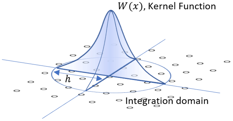
Figure 2 Example of a kernel function used as integration domain for mathematical operations.

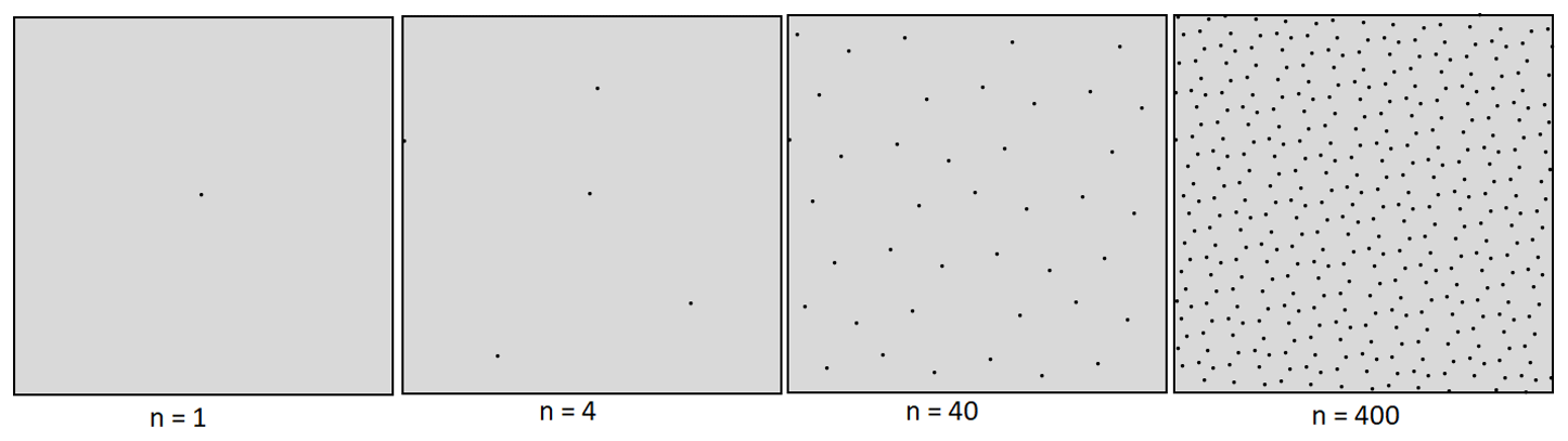
Figure 3 Example particle distributions using the R₂ sequence, note that while not all particles are equidistant, the method produces distributed particle patterns that adapt well to varying density.

Figure 4 The dimensions of the flume experiment setup used in this work.

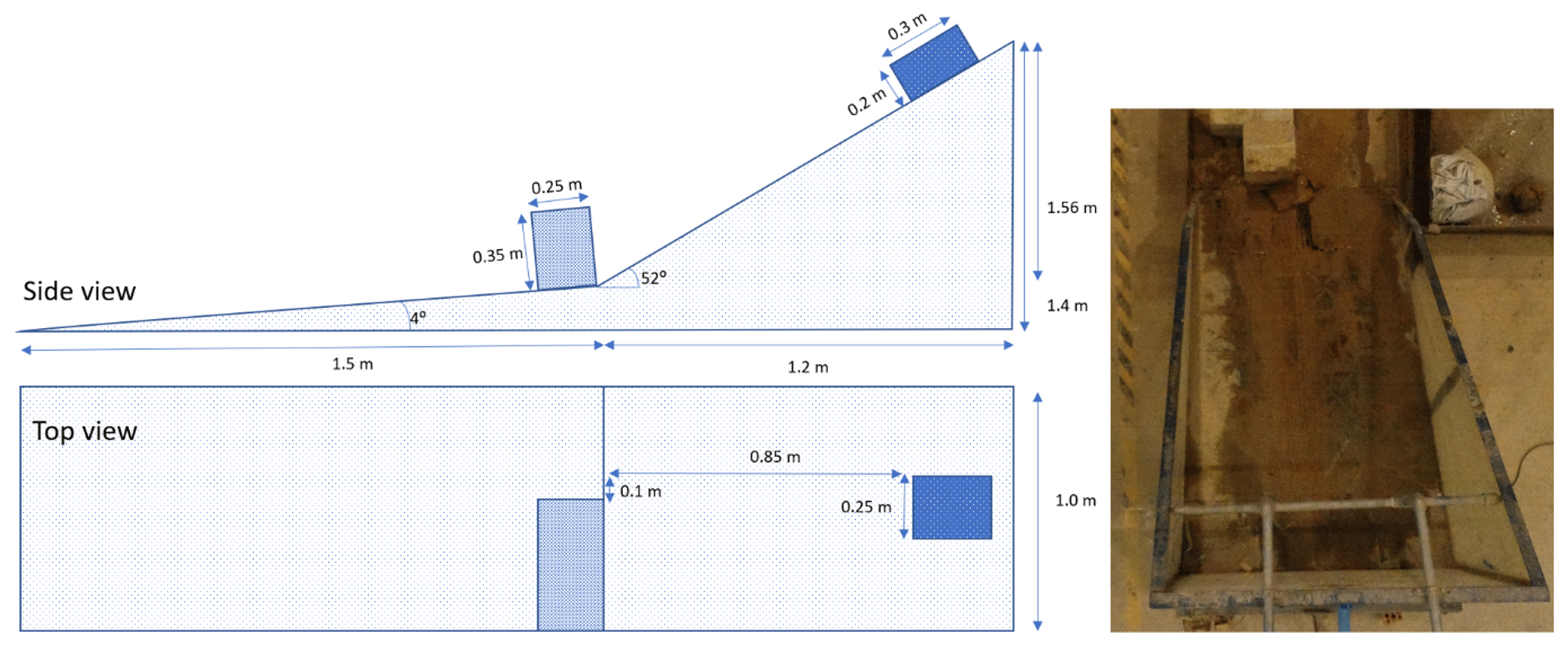
Two tests were performed whereby a cohesive granular matrix was released at the upper part of the flume setup. Both of these volumes had dimensions of $\mathrm{0.2}\times \mathrm{0.3}\times \mathrm{0.25}$ m (height, length, width). For both of these materials, a mixture of high-organic-content silty-clay soils where used. The material's strength parameters were obtained using tri-axial testing (cohesion, internal friction angle Young's modulus and Poisson ratio). The first set of materials properties were c=26.7 kPa and ϕ=28^∘. The second set of materials properties were c=18.3 kPa and ϕ=27^∘. For both of the events, pre- and post-release elevation models were made using photogrammetry. The model was set up to replicate the situations using the measured input parameters. Numerical settings were chosen as follows: $\mathit{\{}{\mathit{\alpha }}_{\mathrm{s}}=\mathrm{0.5},{\mathit{\alpha }}_{\mathrm{f}}=\mathrm{0.5},f_{\mathrm{sc}}=\mathrm{1.0},f_{\mathrm{fc}}=\mathrm{1.0},{\mathit{\rho }}_{\mathrm{f}}=\mathrm{1000}$, ${\mathit{\rho }}_{\mathrm{s}}=\mathrm{2400},E=\mathrm{12}\cdot {\mathrm{10}}^{\mathrm{6}}\mathrm{Pa},K=\mathrm{23}\cdot {\mathrm{10}}^{\mathrm{6}}\mathrm{Pa},\mathit{\psi }=\mathrm{0},{\mathit{\alpha }}_{\mathrm{\Pi }}=\mathrm{1},{\mathit{\beta }}_{\mathrm{\Pi }}=\mathrm{1},X,\mathit{\zeta },j=\mathrm{2},u_{\mathrm{sound}}=\mathrm{600},\mathrm{d}x=\mathrm{10},V_{\mathrm{I}}=\mathrm{0}\mathrm{m}/\mathrm{s},h=\mathrm{10},n=\mathrm{0.1},\mathit{\alpha }=\mathrm{1},\mathit{\beta }=\mathrm{10},M=\mathrm{2.4},\mathcal{B}=\mathrm{0},N_R=\mathrm{15}\mathrm{000},N_{RA}=\mathrm{30}\mathit{\}}$. Calibration was performed by means of input variation. The solid fraction and elastic and bulk modulus were varied between 20 % and 200 % of their original values with increments of 10 %. Accuracy was assessed based on the percentage accuracy of the deposition (comparison of the modelled vs. the observed presence of material).

3.2 Results

Both the mapped extent of the material after flume experiments, as the simulation results are shown in Fig. 5. Calibrated values for the simulations are {α_s=0.45, $E=\mathrm{21.6}\cdot {\mathrm{10}}^{\mathrm{6}}\mathrm{Pa},K=\mathrm{13.8}\cdot {\mathrm{10}}^{\mathrm{6}}\mathrm{Pa}$ }.

Figure 5 A comparison of the final deposits of the simulations and the mapped final deposits and cracks within the material: (from left to right) photogrammetry mosaic, comparison of simulation results to mapped flume experiment, strain, final strength fraction remaining.

As soon as the block of material impacts the obstacle, stress increases as the moving object is deformed. This stress quickly propagates through the object. Within the scenario with lower cohesive strength, as soon as the stress reached beyond the yield strength, degradation of strength parameters took place. In the results, a fracture line developed along the corner of the obstacle into the length direction of the moving mass. Eventually, this fracture developed to half the length of the moving body and severe deformation resulted. As was observed from the tests, the first material experienced a critical fracture, while the second test resulted in moderate deformation near the impact location. Generally, the results compare well with the observed patterns, although the exact shape of the fracture is not replicated. Several reasons might be the cause of the moderately accurate fracture patterns. Other studies used a more controlled setup where uncertainties in applied stress and material properties were reduced. Furthermore, the homogeneity of the material used in the tests can not completely assumed. Realistically, minor alterations in compression used to create the clay blocks have left spatial variation in density, cohesion and other strength parameters.

4 Numerical tests

4.1 Numerical setup

In order to further investigate some of the behaviours of the model and highlight the novel types of mass movement dynamics that the model implements, several numerical tests have been performed. The setup of these tests is shown in Fig. 6.

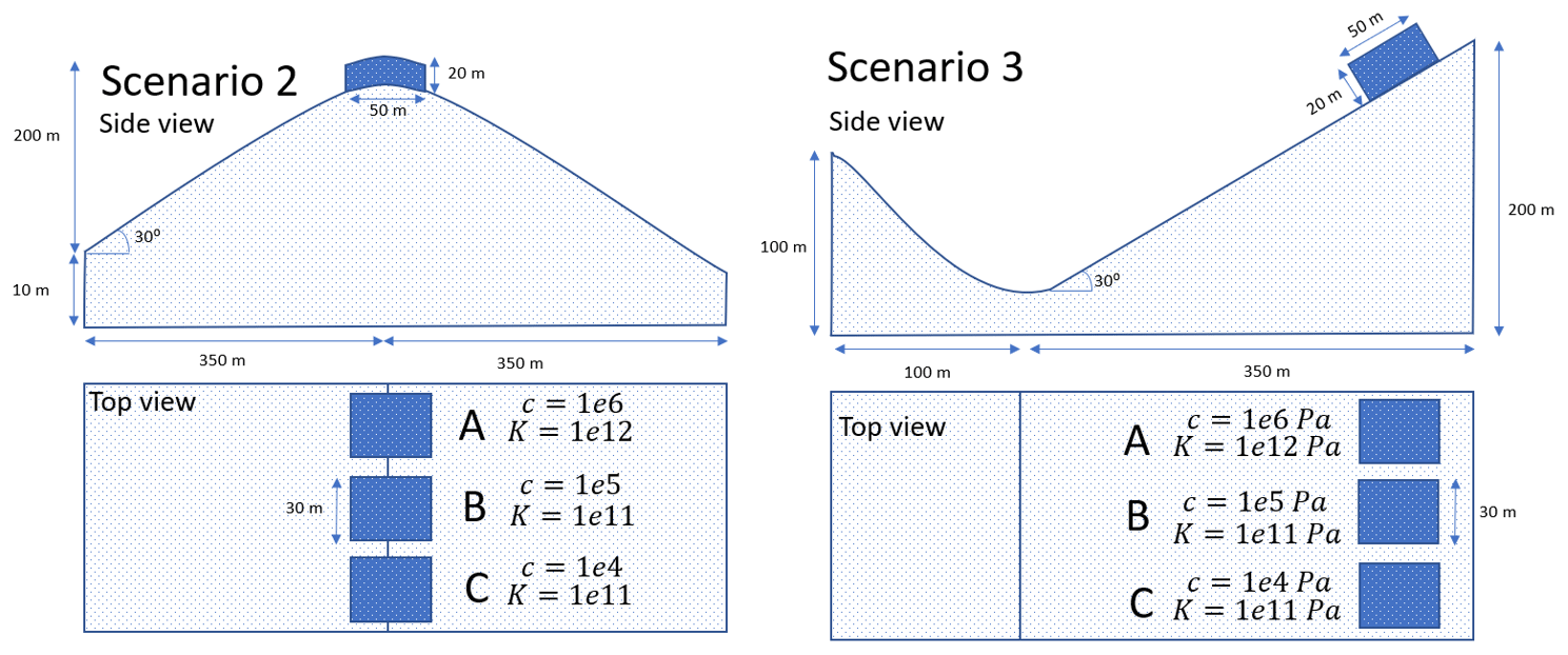
Figure 6 The dimensions of the numerical experiment setups used in this work: setup 1 (left) and setup 2 (right).

Numerical settings were chosen for three different blocks with equal volumes but distinct properties. Cohesive strength and the bulk modulus were varied (see Fig. 6). Remaining parameters were chosen as follows: $\mathit{\{}{\mathit{\alpha }}_{\mathrm{s}}=\mathrm{0.5},{\mathit{\alpha }}_{\mathrm{f}}=\mathrm{0.5},f_{\mathrm{sc}}=\mathrm{1.0},f_{\mathrm{fc}}=\mathrm{1.0},{\mathit{\rho }}_{\mathrm{f}}=\mathrm{1000}\mathrm{kg}{\mathrm{m}}^{-\mathrm{3}}$, ${\mathit{\rho }}_{\mathrm{s}}=\mathrm{2400}\mathrm{kg}{\mathrm{m}}^{-\mathrm{3}},E=\mathrm{1}e\mathrm{12}\mathrm{Pa},\mathit{\psi }=\mathrm{0},{\mathit{\alpha }}_{\mathrm{\Pi }}=\mathrm{1},{\mathit{\beta }}_{\mathrm{\Pi }}=\mathrm{1},X,\mathit{\zeta },j=\mathrm{2},u_{\mathrm{sound}}=\mathrm{600}\mathrm{m}{\mathrm{s}}^{-\mathrm{1}},\mathrm{d}x=\mathrm{10}m,V_{\mathrm{I}}=\mathrm{0}\mathrm{m}/\mathrm{s},h=\mathrm{10}\mathrm{m},n=\mathrm{0.1},\mathit{\alpha }=\mathrm{1},\mathit{\beta }=\mathrm{10},M=\mathrm{2.4},\mathcal{B}=\mathrm{0},N_R=\mathrm{15}\mathrm{000},N_{RA}=\mathrm{30}\mathit{\}}$.

4.2 Results

Several time slices for the described numerical scenarios are shown in Figs. 7 and 8.

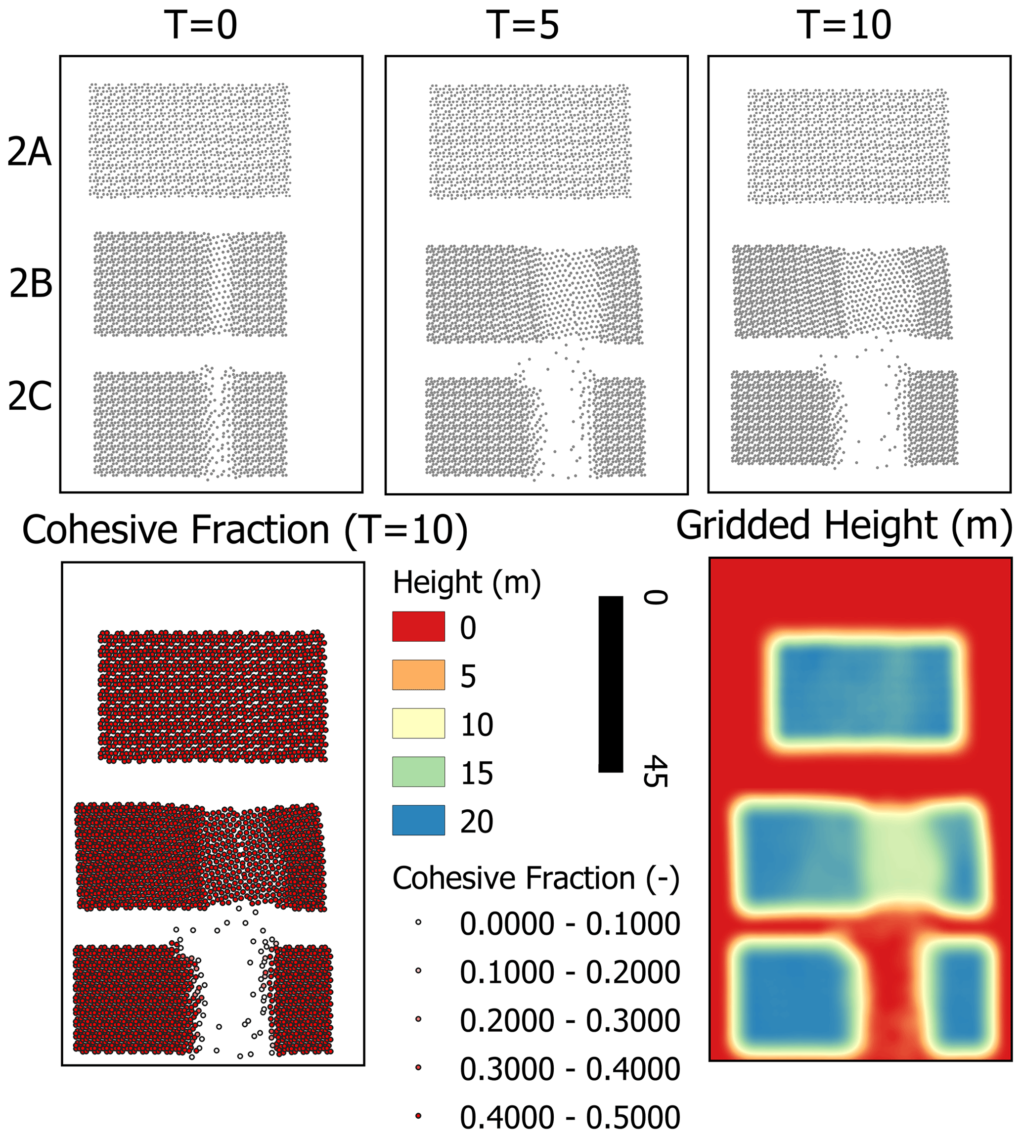
Figure 7 Several time slices for numerical scenarios 2A, 2B and 2C. See Fig. 6 for the dimensions and terrain setup.

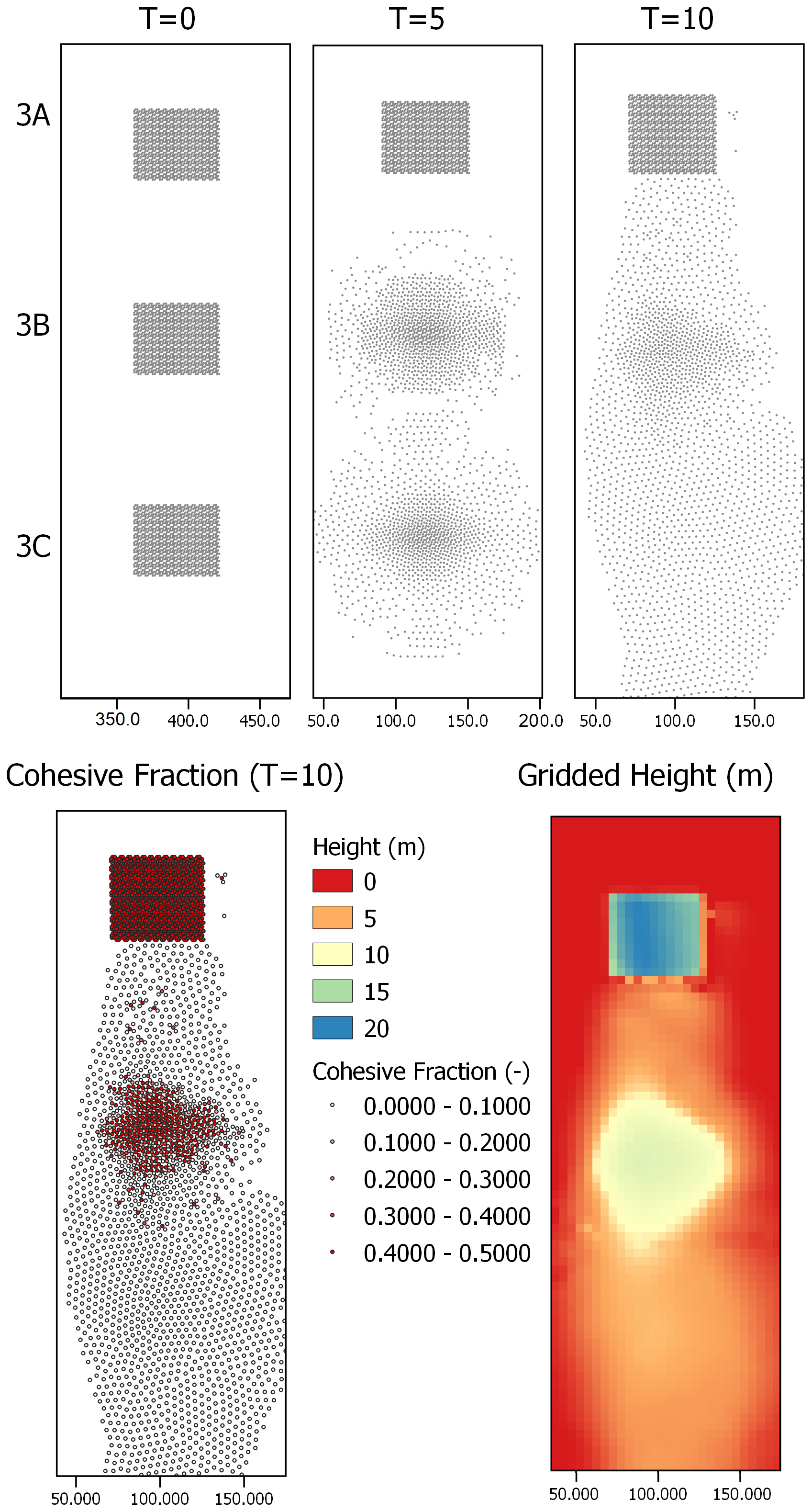
Figure 8 Several time slices for numerical scenarios 3A ,3B and 3C. See Fig. 6 for the dimensions and terrain setup.

Fractures develop in the mass movements based on acceleration differences and cohesive strength. For scenario 2A, the stress state does not reach beyond the yield surface, and all material is moved as a single block. Scenario 2B, which features lowered cohesive strength, fractures and the masses separate based on the acceleration caused by slopes.

Fracturing behaviour can occur in MPM schemes due to numerical limitations inherent in the usage of a limited integration domain. Here, validation of real physically based fracturing is present in the remaining cohesive fraction. This value only reduces in the case of plastic yield, where increasing strain degrades strength parameters according to our proposed criteria. Numerical fractures would thus have a cohesive fraction of 1. In all simulated scenarios, such numerical issues were not observed.

Fragmentation occurs due to spatial variation in acceleration in the case of scenario 3A and 3B. For scenario 3A, the yield surface is not reached and the original structure of the mass is maintained during movement. For 3C, fragmentation is induced by lateral pressure and buoyancy forces alone. Scenario 3B experiences slight fragmentation at the edges of the mass but predominantly fragments when reaching the valley, after which part of the material is accelerated to count to the velocity of the mass. For all the shown simulations, fragmentation does not lead to significant phase separation since virtual mass and drag forces converge the separate phase velocities to their mixture-averaged velocity. The strength of these forces partly depends on the parameters; effects of more immediate phase separation could be studied if other parameters are used as input.

5 Discussion

A variety of existing landslide models simulate the behaviour of lateral connected material through a non-linear, non-Newtonian viscous relationship (von Boetticher et al., 2017; Fornes et al., 2017; Pudasaini and Mergili, 2019; Greco et al., 2019). These relationships include a yield stress and are usually regularized to prevent singularities from occurring. While this approach is incredibly powerful, it is fundamentally different from the work proposed here. These viscous approaches do not distinguish between elastic or plastic deformation and typically ignore deformations if stress is insufficient. Additionally, fracturing is not implemented in these models. The approach taken in this work attempts to simulate a full stress–strain relationship with Mohr–Coulomb type yield surface. This provides new types of behaviour and can be combined with non-Newtonian viscous approaches as mentioned above. A major downside to the presented work is the steep increase in computational time required to maintain an accurate and stable simulation. Commonly, a near 100 times increase in computational time has been observed during the development of the presented model.

The presented model shows a good likeness to flume experiments, and numerical tests highlight behaviour that is commonly observed for landslide movements. There are, however, inherent scaling issues and the material used in the flume experiments is unlikely to form larger landslide masses. The measured physical strength parameters of the material used in the flume experiments would not allow for sustained structured movement at larger scales. There is thus the need for more real-scale validation cases. The application of the presented type of model is most directly noticeable for block-type landslide movements that have fragmented either upon impact with some obstacle or during the transition phase. Of importance here is that the moment of fragmentation is often not reported in studies on fast-moving landslides, potentially due to the complexities involved in knowing the details of this behaviour from post-event evidence. Validation would therefore have to occur in cases where deposits are not fully fragmented, indicating that this process was ongoing during the whole movement duration. The spatial extent of initiation and deposition would then allow validation of the model. Another major opportunity for validation of the novel aspects of the model is the full three-dimensional application to landslides that were reported to have lubrication effects due to fragmentation of the lower fraction of flow due to shear.

An important point of consideration in the development of complex multi-process generalized models is the applicability. As a detailed investigative research tool, these models provide a basic scenario of usage. However, both for research and beyond for applicability in disaster risk reduction decision support, the benefit drawn from these models depends on the practical requirement for parameterization and the computational demands for simulation. With an increasing complexity in the description of multi-process mechanics comes the requirement for more measured or estimated physical parameters. Inspection of the presented method shows that in principle, a minor amount of new parameters are introduced. The cohesive strength, a major focus of the model, becomes highly important depending on the type of movement being investigated. Additionally, the bulk and elastic modulus are required. These three parameters are common simulation parameters in geotechnical research and can be obtained from common tests on sampled material (Alsalman et al., 2015). Finally, the basal pressure propagation parameter (ℬ) is introduced. However, within this work the value of this parameter is chosen to have a constant value of 1. As a result, the model does require additional parameters, although these are relatively easy to obtain with accuracy.

There are a variety of aspects of the model that could be significantly improved. Here, we list several major opportunities for future research.

1. Groundwater mechanics. The presented model allows for the a solid or granular matrix to be present within the flow. We have assumed the flows in and out of these matrices are small enough that they can be ignored. In reality, there is a fluid flux in and out of structured solids. This could occur both due to pressure differences and due to stress and strain of the structured solids. Implementing this kind of mechanic requires a dynamic, solid-properties-dependent, soil water retention curve (Van Looy et al., 2017). An example of MPM soil mechanics with dynamic groundwater implementation can be found in Bandera et al. (2016).

2. Implementing entrainment and deposition. Current equations for entrainment (erosion with major grain-grain interactions) are limited to unstructured mixture flows (Iverson, 2012; Iverson and Ouyang, 2015; Cuomo et al., 2016; Pudasaini and Fischer, 2016). Extending these models to include a contribution from structured solids would be required to implement entrainment in the presented work.

3. Separation of phases. A major assumption in the presented work is that the velocities of structured solids, free solids and confined fluids are all equal. In reality, there might be separation of structured- and free-solid phases. Additionally, we already discussed the possibility of influx and outflux of confined fluids from the solid matrix. Recent innovations in three-phase mixture flows might be used to extend the presented work to a three-, four- or five-phase model by separating free solids and confined fluids or adding a Bingham viscous solid–fluid phase (Pudasaini and Mergili, 2019). However, while this would implement an additional process, it would significantly increase the complexity of the equations (in an exponential manner with relation to the number of phases) and the numerical solutions, which could hinder practical applicability.

4. Application to large slow-moving landslides. When confined fluids would act as a distinct phase guided by the mechanics of water flow in granular matrix, groundwater pressures and movement through the structured solids could be described. This might enable the model to perform detailed deformation and groundwater simulation of large slow-moving landslides.

5. Numerical improvements. Numerical techniques for particle-based discretized methods (SPH, MPM) have been proposed in the literature. A common issue is numerical fracturing of materials when particle strain increases beyond the length of the kernel function. Due to this, the connection between particles is lost, and fracturing occurs as an artefact of the numerical method. This issue is partly solved by the artificial stress term that is also used by Bui et al. (2008). Additionally, a geometric subdivide, as used by Xu et al. (2012) and Li et al. (2015), could counter these artificial fractures. Implementing this technique does require additional work to maintain mass and momentum conservation.

6. Three-dimensional solutions. In a variety of scenarios, the assumptions made in the depth-averaged application of flow models are invalid. A common example is the impact of mass movements into lakes or other large water bodies. In such cases, the vertical velocity and concentration variables are not well described by their depth-averaged counterparts. Additionally, the lubrication effect of basal fragmentation of landslides due to shear can not be described without velocity profiles and a vertical stress solution. A full three-dimensional application would therefore have the potential to increase understanding of these important processes.

6 Conclusions

We have presented a novel generalized mass movement model that can describe both unstructured mixture flows and structured movements of Mohr–Coulomb-type material. The presented equations are part of the continuous development of the OpenLISEM hazard model, an open-source tool for physically based multi-hazard simulations. The model builds on the works of Pudasaini (2012) and Bui et al. (2008) to develop a single holistic set of equations. The model was implemented in a GPU-based material point method (MPM) Code. The equations were validated on flume experiments and numerical tests that highlight the new movement dynamics possible with the presented model. The integration of cohesive structure and a full stress–strain relationship for the structured solids allows for movement of block-type slides as a single whole. Interactions with terrain, other flow masses or obstacles lead to elasto-plastic deformation and eventually fragmentation. This type of self-alteration of flow properties is novel with mass movement models. Although the presented equations can provide additional detail for specific mass movement types, applicability of the model for real events need to be investigated as computational costs are significantly increased.

The presented simulation both validates the basic behaviour of the model and highlights the types of flow dynamics made possible by the presented equations. The model's dependency on cohesive strength and internal friction angles matches the flume experiments. The numerical examples show commonly described behaviour for landslide movements. Although the simulations compare well to the flume experiments, validation is required for real-scale application to various types of mass movements. Additionally, the presented equations still lack descriptions of processes that might become important. Separating the fluid and solid phases (as in Pudasaini and Mergili, 2019) could improve flow dynamics and phase separation. With added groundwater mechanics, such as those in Bandera et al. (2016), slow-moving landslide simulations might be described.

Appendix A: List of symbols

h	flow height
s	solid phase
f	fluid phase
sc	structured solid phase
fc	confined fluid phase
ρf	density of fluids
ρs	density of solids
αf	volumetric fluid-phase fraction
αs	volumetric solid-phase fraction
fsc	fraction of solids that is structured (confining)
ffc	fraction of fluids that is confined
αc	volumetric fraction of solids, structured solids and confined fluids
αu	volumetric fraction of free fluids (unconfined phase).
ρsc	volume-averaged density of the solids and confined fluids
uu	velocity of the unconfined phase (free fluids)
uc	velocity of the solids, confining solids and confined fluids
us	velocity of the solids
f	body force
MDG	drag force
Mvm	virtual mass force
Tc	stress tensor for the solids, confining solids and confined fluids
Tu	stress tensor for the free-fluid phase
σ	stress tensor
$\dot{s}$	deviatoric shear stress rate tensor
δ	Kronecker delta
${\dot{\mathit{ϵ}}}_{\mathrm{plastic}}$	plastic strain rate
${\dot{\mathit{ϵ}}}_{\mathrm{elastic}}$	elastic strain rate
λ	plastic multiplier rate
g	plastic potential function
${\dot{\mathit{ϵ}}}_{\mathrm{total}}$	total strain rate
$\dot{e}$	deviatoric strain rate
ν	Poisson's ratio
E	elastic Young's modulus
G	shear modulus
K	bulk elastic modulus
f(I1,J2)	yield surface or yield criterion
g(I1,J2)	plastic potential function
ψ	dilatancy angle
I1	first stress invariant
J2	second stress invariant
αϕ	first Drucker–Prager material constant
kc	second Drucker–Prager material constant
$\dot{\mathit{\omega }}$	spin rate tensor
ϵv0	initial volumetric strain
ϵv	volumetric strain
c0	initial cohesion
τf	fluid Cauchy stress tensor
pf	fluid pressure
ηf	fluids dynamic viscosity
𝒜	mobility of the fluid at the interface
𝒞DG	drag coefficient
UT,c	settling velocity of the solids, structured solids and confined fluids

UT,uc	settling velocity of the unstructured solids
ℱ	drag contribution from solid-like drag
𝒢	drag contribution from fluid-like drag
Sp	smoothing function
𝒦	absolute total mass flux
M(Rep)	empirical function weakly dependent on the Reynolds number
𝒫	partitioning parameter for the fluid- and solid-like contributions to drag
m	an exponent for P
𝒞VMG	virtual mass coefficient
|S|	norm of the shear force
N	normal force on a plane element
g	gravitational acceleration
$P_{{\mathrm{b}}_{s,u}}$	basal pressure from the unconfined phase
$P_{{\mathrm{b}}_u}$	basal pressure from the free fluids
$P_{{\mathrm{b}}_{\mathrm{c}}}$	basal pressure from the solids, structured solids and confined fluids
ℬ	pressure propagation factor for structured solids
Ka	active lateral earth–pressure coefficient
Kp	passive lateral earth–pressure coefficient
ζ	shape factor for the vertical gradient in solid concentration
n	Manning's surface roughness coefficient
X	shape factor for the vertical fluid velocity profile
Rep	particle Reynolds number
NR	Reynolds number
NRA	interfacial Reynolds number
H	typical height of the flow
L	typical length of the flow
α	first viscosity parameter
β	second viscosity parameter
d	grain diameter
W	kernel weight function
r	distance
h	kernel width (not to be confused with the flow height)
q	normalized particle distance
Πij	an artificial viscosity term
$F_{ij}^n{R}_{ij}^{\mathit{\alpha }\mathit{\beta }}$	an artificial stress term
ϵ0	a constant parameter for the artificial stress term
αΠ and βΠ	constants in the artificial viscous force
usound	speed of sound in the material
N(x)	grid kernel function
cp	plastic coefficient

Appendix B: Stress remapping

If the state of the stress tensor lies beyond the yield surface, either due to degradation of strength parameters or building numerical errors, a correction must be applied. We implement the correction scheme used by Bui et al. (2008). This scheme considers two primary ways in which the stress can have an undesired state: tension cracking and imperfectly plastic stress.

B1 Tension cracking

In the case of tension cracking, the stress state has moved beyond the apex of the yield surface, as described by Chen and Mizuno (1990). The employed solution in this case is to re-map the stress tensor along the I₁ axis to be at this apex. The apex is provided by the following yield function:

$$\begin{array}{}\text{(B1)}& -{\mathit{\alpha }}_{\mathit{\varphi }}{I}_{\mathrm{1}}+k_{\mathrm{c}}<\mathrm{0}.\end{array}$$

To solve for this condition, the non-deviatoric stress state is increased (since $I_{\mathrm{1}}-\frac{k_{\mathrm{c}}}{{\mathit{\alpha }}_{\mathit{\varphi }}}$ is negative) to lie perpendicular to the apex point on the I₁ axis as follows:

$$\begin{array}{}\text{(B2)}& \stackrel{\mathrm{̃}}{{\mathit{\sigma }}^{\mathit{\gamma }\mathit{\gamma }}}=r{s}^{\mathit{\gamma }\mathit{\gamma }}-{\displaystyle \frac{\mathrm{1}}{\mathrm{3}}}\left(I_{\mathrm{1}}-{\displaystyle \frac{k_{\mathrm{c}}}{{\mathit{\alpha }}_{\mathit{\varphi }}}}\right).\end{array}$$

B2 Imperfect plastic stress

Imperfect plastic stress described the state where the stress tensor lies above the apex but beyond the yield criterion and thus have more stress than is supported by the failure criteria that is set. This criterion is simply the yield surface itself (Eq. B3).

$$\begin{array}{}\text{(B3)}& -{\mathit{\alpha }}_{\mathit{\varphi }}{I}_{\mathrm{1}}+k_{\mathrm{c}}<\sqrt{J_{\mathrm{2}}}\end{array}$$

For this state, re-mapping is done by scaling of the J₂ value (Eqs. B4, B5 and B6).

$$\begin{array}{}\text{(B4)}& {\displaystyle }r={\displaystyle \frac{-{\mathit{\alpha }}_{\mathit{\varphi }}{I}_{\mathrm{1}}+k_{\mathrm{c}}}{\sqrt{J_{\mathrm{2}}}}}\text{(B5)}& {\displaystyle }\stackrel{\mathrm{̃}}{{\mathit{\sigma }}^{\mathit{\gamma }\mathit{\gamma }}}=r{s}^{\mathit{\gamma }\mathit{\gamma }}+{\displaystyle \frac{\mathrm{1}}{\mathrm{3}}}{I}_{\mathrm{1}}\text{(B6)}& {\displaystyle }\stackrel{\mathrm{̃}}{{\mathit{\sigma }}^{xy}}=r{s}^{xy},\stackrel{\mathrm{̃}}{{\mathit{\sigma }}^{xy}}=r{s}^{xz}\stackrel{\mathrm{̃}}{{\mathit{\sigma }}^{xy}}=r{s}^{yz}\end{array}$$

Appendix C: Software implementation

The model presented in this article is part of the continued development of the OpenLISEM modelling tools. The most recent set of equations were implemented in the open-source alpha version of OpenLISEM hazard model 2.0a. Here we describe the details of the implementation of the model into software.

C1 Hybrid MPM

We utilize the MPM framework to be able to discretize part of the equations on a Eulerian regular grid and part of the equations on the Lagrangian particles. Our distinct take on this method is the representation of the fluid phase entirely as a finite-element solution, while solids are simulated as discrete particle volumes. This allows the model to use the major benefits that are present when depth-averaged fluid flow is simulated in a grid. Both numerical efficiency and high-accuracy coupling with hydrology are lacking in particle methods. For the solid phase, non-dissipative advection, fracturing and stiffness is a major benefit of the MPM approach. Since our model assumed that confined fluids share their velocity with the solids, we advect the confined fluids as part of the particles. Total fluid volume is then calculated from the free fluids in the finite-element data and the gridded particle data. A flow chart of the software setup is provided in Fig. 6.

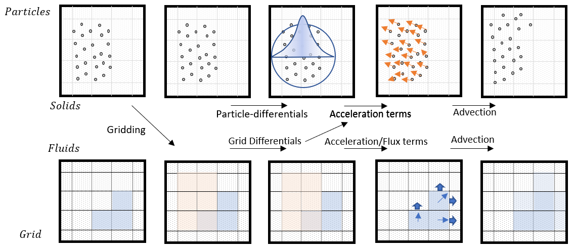
Figure C1 The sub-steps taken by the software to complete a single step of numerical integration.

C2 Finite-element solution

We use a regular Cartesian grid to describe the modelling domain. Terrain and cell-boundary-based variables are reproduced using the Monotonic Upstream-centered Scheme for Conservation Laws (MUSCL) piecewise linear reconstruction (Delestre et al., 2014). For each cell boundary, a left and right estimation of acceleration terms, velocity updates, and new discharges is made. The left estimates use left-reconstructed variables, while the right estimates use right-reconstructed variables. The final average flux through the boundary determines the actual mass and momentum transfer. Local acceleration is averaged from the right estimate of the left boundary and left estimate of the right boundary. An additional benefit of the used scheme is the automatic estimation of continuous and discontinuous terrain. The piecewise linear reconstructions do not guarantee smooth terrain; for sharp locally variable terrain, pressure terms from vertical walls arise that block momentum. These terms allow for better estimation of momentum loss by barriers but can be turned off if required for the simulated scenario.

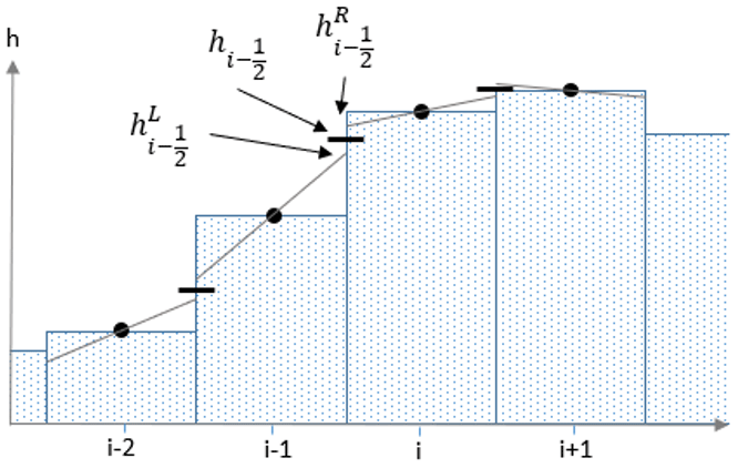
Figure C2 Piecewise linear reconstruction is used by the MUSCL scheme to estimate values of flow heights, velocities and terrain at cell boundaries.

C3 GPU acceleration using OpenCL/OpenGL

In order to create a more efficient setup, both the finite-element and particle interactions are performed on the GPU. We utilize the OpenCL API to compile kernels written in C-style language. These kernels are compiled at the start of the simulation and thereby allow for easy customization by users. While the usage of OpenCL 1.1 forces the usage of single precision floating point numbers, it allows for a wider range of GPU types to be supported. Finite-element solutions on the GPU are straightforward, as maps are a basic data storage type for graphical processing units. Particles are stored as single precision floating point arrays. Within the framework of MPM, iteration of particles within a kernel is required for each time step and particle. This effectively means O(n²) operations are required. Significant efficiency improvements are obtained by pre-calculation sorting. Particles are sorted based on their location within the finite-element grid. Based on the ID of the grid cell, a bitonic mergesort is performed. This sorting algorithm works seamlessly on parallel architecture and operates as O(nlog ²(n)) (Batcher, 1968). Following this, a raster is allocated to store the first indexed occurrence within the sorted list of particles of that grid cell. Since the kernel used for the presented work extends at most to a full width of two grid cells, we must iterate over all particles present in nine neighbouring grid cells.

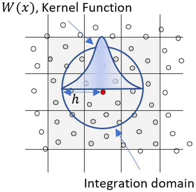
Figure C3 By limiting the kernel and sorting particles before calculation, only the distance of particles in neighbouring cells need to be checked, significantly reducing computational load, particularly for larger datasets.

A final benefit to the usage of OpenCL is direct access to simulation variables for visualization in OpenGL using the OpenGL/OpenCL interoperability functionality. The built-in viewing window of OpenLISEM hazard 2.0a directly uses the data to draw particles, shapefiles and grid data using customizable shaders written in the OpenGL shader language.