the Creative Commons Attribution 4.0 License.
the Creative Commons Attribution 4.0 License.
 | 01 Apr 2021
Improved representation of river runoff in Estimating the Circulation and Climate of the Ocean Version 4 (ECCOv4) simulations: implementation, evaluation, and impacts to coastal plume regions
Dimitris Menemenlis
Huijie Xue
Hong Zhang
Dustin Carroll
In this study, we improve the representation of global river runoff in the Estimating the Circulation and Climate of the Ocean Version 4 (ECCOv4) framework, allowing for a more realistic treatment of coastal plume dynamics. We use a suite of experiments to explore the sensitivity of coastal plume regions to runoff forcing, model grid resolution, and grid type. The results show that simulated sea surface salinity (SSS) is reduced as the model grid resolution increases. Compared to Soil Moisture Active Passive (SMAP) observations, simulated SSS is closest to SMAP when using daily, point-source runoff (DPR) and the intermediate-resolution LLC270 grid. The Willmott skill score, which quantifies agreement between models and SMAP, yields up to 0.92 for large rivers such as the Amazon. There was no major difference in SSS for tropical and temperate coastal rivers when the model grid type was changed from the ECCO v4 latitude–longitude–polar-cap grid to the ECCO2 cube–sphere grid. We also found that using DPR forcing and increasing model resolution from the coarse-resolution LLC90 grid to the intermediate-resolution LLC270 grid elevated the river plume area, volume, stabilized the stratification and shoal the mixed layer depth (MLD). Additionally, we find that the impacts of increasing model resolution from the intermediate-resolution LLC270 grid to the high-resolution LLC540 grid are regionally dependent. The Mississippi River Plume is more sensitive than other regions, possibly because the wider and shallower Texas–Louisiana shelf drives a stronger baroclinic effect, as well as relatively weak sub-grid vertical mixing and adjustment in this region. Since rivers deliver large amounts of freshwater and anthropogenic materials to coastal regions, improving the representation of river runoff in global, high-resolution models will advance studies of coastal hypoxia, carbon cycling, and regional weather and climate and will ultimately help to predict land–ocean–atmospheric feedbacks seamlessly in the next generation of Earth system models.
- Article
(2992 KB) - Full-text XML
-
Supplement
(1526 KB) - BibTeX
- EndNote


Coastal plume regions represent a small fraction of Earth's surface and are an active component in global cycling of carbon and nutrients (Bourgeois et al., 2016; Carroll et al., 2020; Fennel et al., 2019; Lacroix et al., 2020; Landschützer et al., 2020; Roobaert et al., 2019). Recent satellite-based observations with quasi-global coverage have been greatly improved to monitor sea surface salinity (SSS), a key tracer for tracking the river plumes. The European Space Agency (ESA) Soil Measure and Ocean Salinity (SMOS; Mecklenburg et al., 2012) with 33 km–10 d space–time gridding and National Aeronautics and Space Administration (NASA) Soil Moisture Active Passive (SMAP) missions with 40 km–8 d space–time gridding are acquiring SSS observations with sufficient resolution to track the plume pathways and evaluate coastal plume dynamics (Fournier et al., 2016a, b, 2017a, b, 2019; Gierach et al., 2013; Liao et al., 2020). To date, however, the coastal plume regions have not been explicitly resolved in most global ocean general circulation models (OGCMs), Earth system models (ESMs), and Global Ocean Data Assimilation System (GODAS) products (Ward et al., 2020). As a result, the plume region produced by OGCMs, ESMs, and GODAS are not consistent with satellite observations. For example, Fournier et al. (2016a) found that the ∘ global circulation Hybrid Coordinate Ocean Model (HYCOM) did not accurately capture SSS during extreme flood events in the northern Gulf of Mexico. Denamiel et al. (2013) found that the Congo River nearshore SSS in global HYCOM was underestimated compared to other regional simulations, even though the models had comparable horizontal grid resolution. Santini and Caporaso (2018) suggested that most CMIP5 models might lack skill in representing the Congo River Basin runoff and SSS in the vicinity of river mouths. Most OGCMs, ESMs, and GODAS products usually had large grid cells; a few cells may encompass the entire plume. As a result, water delivered to the cells are fully mixed and diluted and therefore cannot accommodate the complex dynamics. Additionally, riverine freshwater input to the ocean is forced in the top model layer over a pre-determined surface area in the vicinity of river mouths with climatological signal; thus the system disturbance by extreme weather events, e.g., floods and droughts, cannot been explicitly resolved (Griffies et al., 2005; Tseng et al., 2016). Finally, virtual salt fluxes (VSFs) have been widely employed, where freshwater affects salinity without a change in mass or volume flux (Bentsen et al., 2013; Halliwell, 2004; Timmermann et al., 2009; Volodin et al., 2010). The above model configurations may limit the representation of coastal plume regions in global-scale models.
Estimating the Circulation and Climate of the Ocean (ECCO) is a data-assimilating model that uses observational data to make the best possible estimates of ocean circulation and its role in climate. The model takes the cube–sphere (ECCO2) to latitude–longitude–polar-cap (ECCOv4) grids for global application. Like most OGCMs, ESMs, and GODAS products, the current ECCO routes riverine freshwater from land directly to the ocean by taking observed river runoff as seasonal climatology mass flux over the top of several surface grid cells near the river mouths (Fekete et al., 2002; Stammer et al., 2004). Recent ECCO efforts have been extended to address the global-ocean estimates of pCO2 and air–sea carbon exchange (Carroll et al., 2020), and model resolution as fine as 1 km has been promoted globally to investigate mesoscale-to-submesoscale dynamics in the open ocean (Su et al., 2018). However, current ECCO lacks representation of coastal interfaces and related feedbacks limiting their predictability to global climate change, and this may further impede our ability to make informed resource management decisions. In this study, we improve the representation of river runoff in the ECCO and systematically evaluate model performance in reproducing SSS within the vicinity of large tropical and temperate river mouths. We also investigate the impact of runoff forcing, model grid resolution, and grid type on coastal dynamics and critical physical properties near the plume regions. The goal of this work is to provide a comprehensive sensitivity analysis of runoff forcing in multiple simulations, which will aid in the development of global ECCO that more robustly reflecting the land–ocean aquatic continuum (LOAC).
The paper is organized as follows. Section 2 briefly introduces the ECCO model and the various runoff forcing methods used in this study. Section 3 provides a comprehensive evaluation of model sensitivity to horizontal grid resolution and river forcing. Section 4 discusses the sensitivity of plume properties and coastal stratification. Results are summarized in Sect. 5.
2.1 ECCO simulations and representation of river runoff
In this study, we employ the Massachusetts Institute of Technology general circulation model (MITgcm; Marshall et al., 1997) in a number of model configurations that have been developed for the ECCO project (Menemenlis et al., 2005; Forget et al., 2015; Zhang et al., 2018). The ECCO MITgcm configurations that we use herein solve the hydrostatic, Boussinesq equations on either cube–sphere (CS; Adcroft et al., 2004) or latitude–longitude–polar-cap (LLC; Forget et al., 2015) grids. The cube–sphere configuration that we use is the so-called CS510 grid, which was developed for the ECCO2 project (Menemenlis et al., 2008), consists of 6 faces with 510 × 510 dimension, and has quasi-homogeneous horizontal grid spacing of 20 km. We also consider three different LLC grid configurations: LLC90, LLC270, and LLC540, which have, respectively, 1∘, ∘, and ∘ nominal horizontal grid spacing. The LLC grids are aligned with lines of latitude and longitude between 70∘ S and 57∘ N and are locally isotropic with grid spacing varying with latitude. In the tropics, the LLC grid is refined in the meridional direction to better resolve zonal currents. At high latitudes, the LLC grid is adapted to a two-dimensional conforming mapping algorithm for spherical geometry. For our experiments, we use LLC# horizontal grids, where the # is the number of points along one-quarter of the Equator. Therefore, LLC90 means 360 grid points circle the Equator. The model has 50 vertical z levels; vertical resolution is 10 m in the top 7 levels and telescopes to 450 m at depth. This setup was the same for all designed experiments. We use a third-order, direct-space–time (DST-3) advection scheme, while vertical advection uses an implicit third-order upwind scheme. Vertical mixing is parameterized using the Gaspar–Grégoris–Lefevre (GGL) mixing-layer turbulence closure and convective adjustment scheme (Gaspar et al., 1990). Lateral eddy viscosity in ECCOv4 is harmonic, with a coefficient of , where L is the grid spacing in meters and Δt=3600 s. Depending on location, the resulting eddy viscosity varies from ∼103 to m2 s−1. Additional sources of dissipation in ECCOv4 are from harmonic vertical viscosity and quadratic bottom drag, along with contributions from the vertical mixing parameterization. A detailed description of ECCOv4 is provided in Forget et al. (2015).
ECCOv4 uses natural boundary conditions for the surface freshwater fluxes (Huang, 1993; Roullet and Madec, 2000), in which runoff is applied as a real freshwater flux forcing, which allows for material exchanges through the free surface and more precise tracer conservation compared to virtual salt flux boundary conditions (Campin et al., 2008). The model uses z∗ rescaled-height vertical coordinates (Adcroft and Campin, 2004) and the vector-invariant form of the momentum equation (Adcroft et al., 2004). With z∗ coordinates, variability in free surface height is distributed vertically over all grid cells. For a water column that extends from the bottom at to the free surface at z=η, the z∗ vertical coordinate is defined as , where is the rescaling factor. The Boussinesq, depth-dependent equations for conservation of volume and salinity under the vector-invariant form of the momentum equations are
where F is the surface freshwater flux (includes both precipitation minus evaporation and river runoff), and ∇z∗ is the gradient operator on the z∗ plane. S is the potential salinity, Dv,S and Dσ,S are subgrid-scale vertical and horizontal iso-neutral mixing, and vres and wres are the horizontal and vertical residual mean velocity fields. Our daily, point-source runoff (DPR) experiments added freshwater to a single model grid cell in the first vertical model layer, while the diffuse climatological runoff experiments added it over multiple horizontal grid cells in the top layer. The amount of freshwater added to each model grid cell decreased exponentially as a function of distance from river outlets.
2.2 Sensitivity experiments
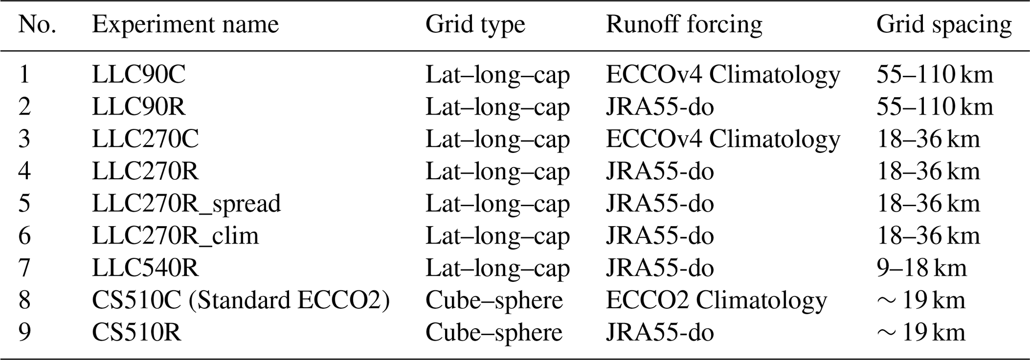
We first run seven experiments, derived from the ECCOv4 setup, to test the sensitivity of SSS in the vicinity of large river mouths to ECCOv4 model grid resolution and runoff forcing (Table 1). The LLC90, LLC270, and LLC540 correspond to coarse (1∘ – ∼ 100 km), intermediate (∘ – ∼ 40 km), and high (∘ – ∼20 km) resolution from low latitudes to mid-latitudes. LLC90C and LLC270C are forced by monthly climatological runoff from Fekete et al. (2002). The runoff has a spatial resolution of ∼ 1∘ and has been linearly interpolated to each grid cell. Therefore, runoff may be fluxed into a single grid cell in the coarse-resolution run and over several grid cells in the high-resolution run. The twin experiments, LLC90R and LLC270R, as well as the highest resolution run LLC540R, use the Japanese 55-year atmospheric reanalysis (JRA55-DO) river forcing dataset (Suzuki et al., 2017; Tsujino et al., 2018). JRA55-DO includes daily river runoff generated by running a global hydrodynamic model forced by adjusted land-surface runoff. Compared to the Fekete ECCOv4 runoff, JRA55-DO runoff has daily output; therefore, it can resolve interannual variability and extreme floods and drought events. We add JRA55-DO runoff as point source flux at a single grid cell adjacent to river outlets. For the intermediate-resolution LLC270 run, we did two additional experiments LLC270R_spread and LLC270R_clim. The LLC270R_spread used daily JRA55DO runoff, but over several grids by allowing the model automatic interpolation onto model grids. The LLC270C_clim used single grid cell point-source surface forcing, but climatological runoff derived from 2015 to 2017. The additional experiments were taken because the widely used climatological Fekete et al. (2002) runoff in ECCOv4 are different from JRA55DO taking the climatology. A comparison between LLC90C vs. LLC270C or LLC90R vs. LLC270R vs. LLC540R shows the resolution impact, while a comparison between LLC270R_spread and LLC270R shows the pure differences by adding runoff to a single grid cell (point-source runoff) and multiple grid cell (diffusive runoff). In addition to the LLC grid, two additional experiments are conducted on the widely used cube–sphere ECCO2 grid to investigate model sensitivity to the choice of grid topology (Table 1). CS510C is an ECCO2 run with monthly climatological runoff from Stammer et al. (2004). The Stammer runoff is spread over a pre-determined surface area in the vicinity of river mouths. The spreading radius decreases exponentially with a 1000 km e-folding distance. Spatial fields of runoff forcing for ECCOv4, ECCO2, and JRA55-DO are shown in Fig. S1 in the Supplement.
Table 1Summary of all experiments. The ECCOv4 and ECCO2 climatological runoff is derived from Fekete et al. (2002) and Stammer et al. (2004), respectively. A comparison of runoff forcings is shown in Fig. S1.
Each sensitivity experiment is integrated for 26 years (1992–2017), and we analyze the final 3-year period (1 January 2015 to 31 December 2017). We begin our analysis in January 2015 because the high-resolution SMAP observations, which we use to evaluate model skill, are available from 1 April 2015. A total of 10 large rivers at 8 coastal regions spanning from low latitudes to mid-latitudes are selected for detailed analysis; these include the Amazon and Orinoco (AZ), Congo (CG), Changjiang (CJ), Ganges and Brahamptura (GB), Mississippi (MR), Parana (PA), Mekong (MK), and Columbia (CO) rivers (Fig. 1).
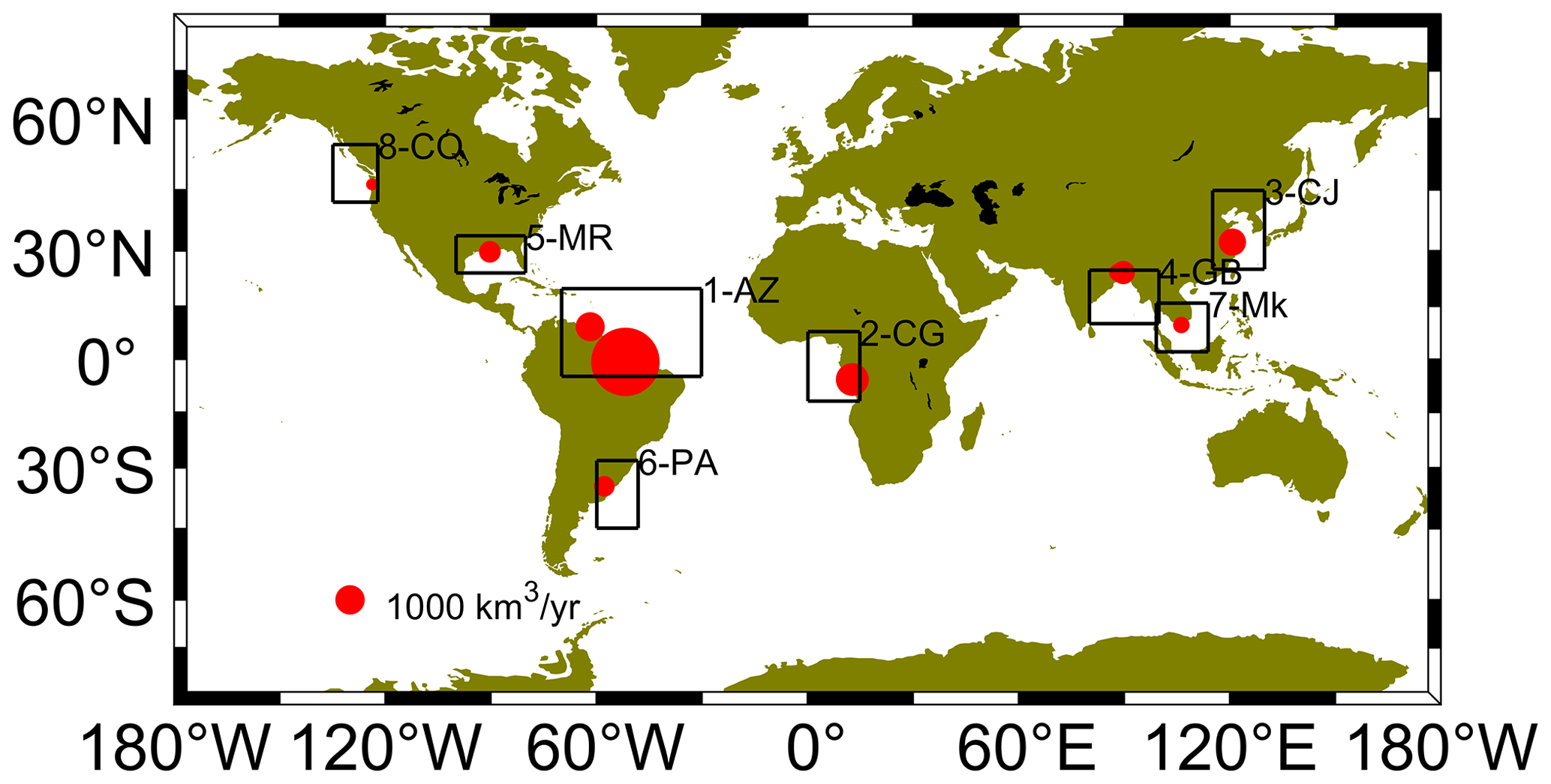
Figure 1The 10 large rivers (red circles) at 8 coastal regions (black boxes) used in our analysis: Amazon and Orinoco (South America, noted as region 1), Congo (Africa, region 2), Changjiang (Asia, region 3), Ganges and Brahamptura (Asia, region 4), Mississippi (North America, region 5), Parana (South America, region 6), Mekong (Asia, region 7), Columbia (North America, region 8). Red circle size is scaled by the climatological river discharge magnitude.
2.3 Target diagram and Willmott skill score
The first part of our study compares the simulated salinity with the synchronized SMAP SSS observations from 1 April 2015 to 31 December 2017. The level-3 SMAP version-3 SSS was produced by the Jet Propulsion Laboratory (ftp://podaac-ftp.jpl.nasa.gov, last access: 29 March 2021; Yueh et al., 2013, 2014). We also compare climatological SSS during this period with the World Ocean Atlas 2018 (https://www.nodc.noaa.gov/OC5/woa18/, last access: 29 March 2021). For quantitative comparison, we use the Willmott skill score (Willmott, 1981), a widely used metric for quantifying agreement between models and observations. The Willmott score is calculated as
where Mi is the model estimate at ti, Oi is the observation at time ti, is the mean of the observations, and n is the number of time records for comparison. Specifically, Wskill=1 indicates perfect agreement between model and observations; Wskill=0 indicates that the model skill is equivalent to the observational mean.
Furthermore, we conduct our skill assessment for model SSS on multiple experiments across several regions. We also use target diagrams (Jolliff et al., 2009) to efficiently visualize a suite of skill metrics. Target diagrams are plotted in a Cartesian coordinate system with the x axis representing the unbiased root-mean-square deviation (RMSD); the y axis represents the bias, and the distance between the origin and any point within the Cartesian space represents total RMSD.
represents the mean of the model estimates. These three skill assessment statistics are particularly useful as bias reports of the size of the model–observation discrepancies. Bias values near zero indicate a close match, though it can be misleading, as negative and positive discrepancies can cancel each other. The unbiased RMSD removes the mean and is a pure measure of how model variability differs from observational variability. The total RMSD provides an overall skill metric, as it includes components for assessing both the mean (bias) and the variability (unbiased RMSD).
We normalize the bias, unbiased RMSD, and total RMSD by the observational standard deviation (σ0) to allow for the display of multiple experiment and regional SSS observations on a single target diagram. According to the definition of unbiased RMSD, the value should always be positive. However, the X<0 region of the Cartesian coordinate space may be utilized if the unbiased RMSD is multiplied by the sign of the standard deviation difference (σd):
The resulting target diagram thus provides information about whether the model standard deviation is larger (X>0) or smaller (X<0) than the observation's standard deviation, in addition to if the model mean is larger (Y>0) or smaller (Y<0) than the observation's mean.
2.4 Definition of plume characteristics
We investigate the role of grid resolution and runoff forcing using several key metrics: plume area, volume, and freshwater thickness. The plume area is defined as regions with SSS below a given salinity threshold SA (See Sect. 4.2). The freshwater volume, relative to the reference salinity, S0, is defined as the integral of the freshwater fraction:
where the volume integral is bounded by the isohaline SA. Here, we assume the maximum salinity in each selected region is the reference salinity S0. The freshwater thickness δfw represents the equivalent depth of freshwater and is computed as
S(z) is the depth-dependent diluted salinity due to the river discharge, η is the sea level, and h is the bottom depth.
We first estimate how the various ECCOv4 LLC simulations (Table 1) compare to observations in the vicinity of 10 large river mouths. The synchronized SMAP SSS (1 April 2015 to 31 December 2017, 33-month) is used as the main verification dataset (Yueh et al., 2013, 2014). SMAP SSS has been documented to exhibit bias compared to observed SSS in shallow waters near river mouths (Fournier et al., 2017a). Therefore, as an indication of absolute SSS, we also compare the model simulations to the World Ocean Atlas 2018 (WOA18). We note that there may be relatively few observations incorporated into the objectively analyzed WOA18 product near the coast, which may over-smooth salinity fronts. Additionally, WOA18 is a 55-year climatology from 1955–2010; therefore, we can only compare model climatology from 2015–2017. Overall, we use SMAP and WOA18 as “observational references”, where our model–observation comparisons provide useful information on how SSS changes between experiments rather than determine which experiment is closer to the real world.
The upper 10 m SSS biases relative to SMAP, averaged over the 33-month period, for CS510C (standard ECCO2) as well as the LLC540R (highest resolution) are shown in Fig. S2. Both SMAP and WOA18 have ∘ horizontal grid resolution; therefore, we interpolated all model fields to this grid. For both simulations, negative biases are found from low latitudes to mid-latitudes, while positive biases occur at high latitudes. When focusing on large river mouth regions (e.g., AZ, PA, and CJ), the SSS bias is reduced in LLC540R. This demonstrates that the choice of runoff forcing impacts SSS at predominantly local scales; however, background currents can transport the signal downstream or offshore to the open ocean (Liu et al., 2009; Molleri et al., 2010).
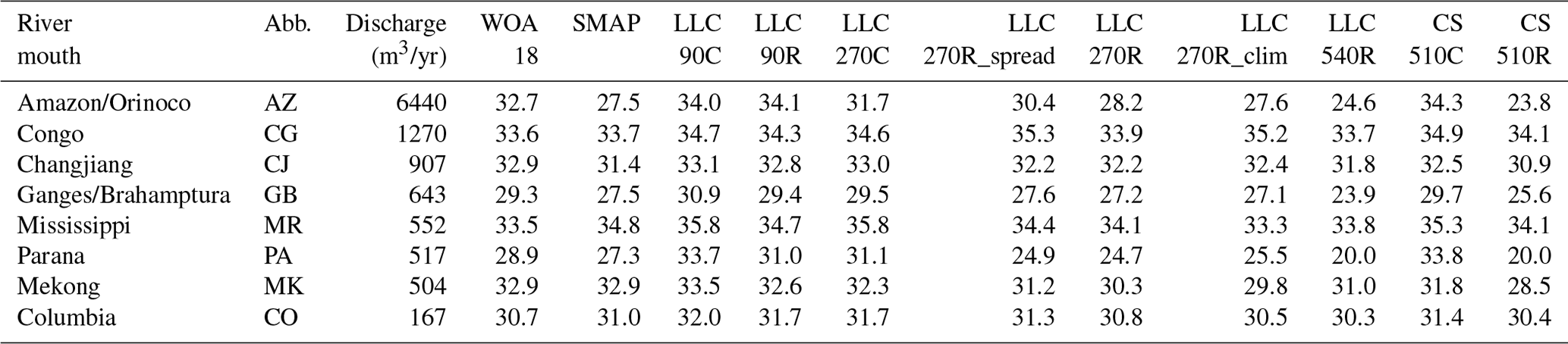
Next, we compute mean model SSS near all selected river mouth regions, along with SMAP and WOA18 (Table 2). The corresponding Willmott skill (WS) numbers are listed in Table 3. We use the first empirical orthogonal function (EOF) derived from WOA18 to determine river mouth regions, since WOA18 represents persistent low-salinity zones over the 30-year period. We remove the mean SSS field before the EOF analysis. The first mode explains ∼ 47 %–67 % of the total variance. We then reconstruct the dominant SSS anomaly field by multiplying the first PC with the spatial pattern. Locations with salinity that is 1–2 PSU lower in the reconstructed SSS field are taken as the river mouth region, and all eight regions are shown in Fig. S3. We first found that SMAP SSS is lower than WOA18 for large rivers. The underestimation is high over 5 PSU for the Amazon region. The deviation between satellite products and in situ observations is consistent with Fournier et al. (2016b, 2017a). Near the selected large river mouths, experiments with daily, point-source runoff forcing generally have lower SSS than experiments forced by climatological diffusive runoff (LLC90R vs. LLC90C; LLC270R vs. LLC270C; CS510R vs. CS510C). Increasing model resolution generally results in regions becoming fresher (Table 2; LLC90C to LLC270C; LLC90R to LLC270R to LLC540R). With the intermediate resolution, the diffusive daily JRA55DO runoff forcing LLC270R_spread had lower salinity than the climatological Fekete-driven forcing run (LLC270C). This is not surprise, since the Fekete river discharge file is more spatially spread than JRA55DO before the model automatic interpolation (Fig. S1), which means less freshwater has been input to the top of the river mouth region, resulting a relatively high salinity. Meanwhile, with the daily JRA55DO forcing, the sea surface salinity with the point-source forcing (LLC270R) was lower than that with the diffusive forcing (LLC270R_spread). It is possible that decreasing the number of cells adding the freshwater was equivalent to decreasing the river mouth inlet width, which results in the inflow velocity increasing and thus spreads the riverine water more widely. In contrast, we found the point-source river forcing run using year-by-year JRA55DO and climatological JRA55DO shows a lack of consistency in SSS change compared to the above two cases.
Table 2The SSS near river mouth for WOA18, SMAP, and all experiments for the selected regions.
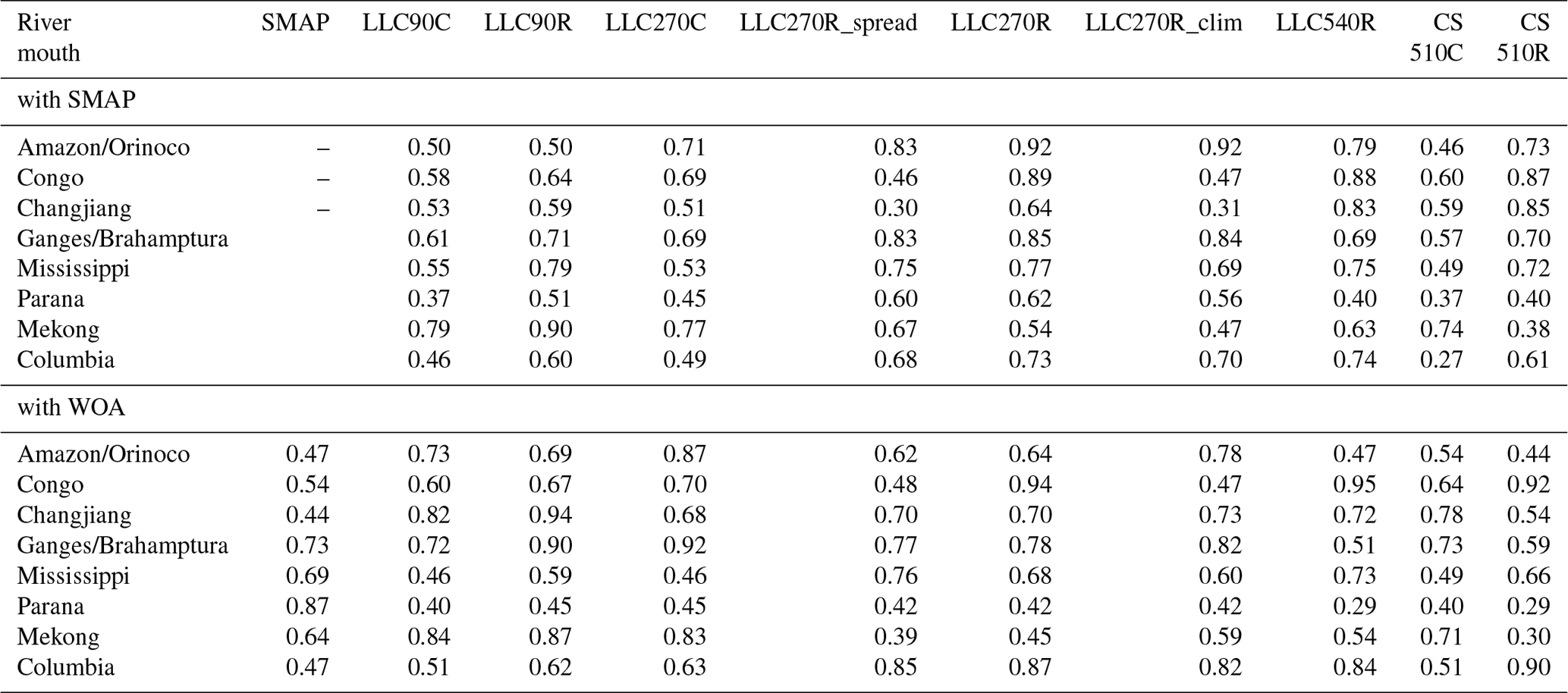
A comparison with SMAP shows that Wskill scores become higher when model resolution increases from 1 to ∘ (LLC90C vs. LLC270C, LLC90R vs. LLC270R), but lower when it increases further to ∘ (e.g., LLC270R vs. LLC540R for Amazon, Ganges/Brahmaputra, Parana). The higher or lower Wskill score is consistent with the SSS decrease. At the AZ region, SSS from LLC270R is less than 1 PSU lower than the SMAP average, while that from LLC540R is roughly 3 PSU lower. Therefore, LLC270R receives a skill score of 0.92, higher than LLC540R (0.74). Although the SSS reduction lowers the model score overall, we should note that SMAP only has ∘ resolution. This means it may not have the capability to resolve those fine-scale dynamic feathers of the plume compared to high-resolution model simulation. In addition, SMAP may underestimate SSS near the river mouth. Therefore, a larger discrepancy with SMAP in the high-resolution run does not indicate that the simulation deviates from the truth.
The Wskill scores when taking SMAP as the reference show that LLC270R_spread is better than LLC270C for AZ, GB, MR, PA, and CO. This is not surprising since the JRA55DO runoff had better temporal resolution than Fekete runoff. Meanwhile, Wskill scores of LLC270R_spread is worse than LLC270R, mainly because of diffusive surface runoff bringing higher SSS than point-source surface runoff (Fig. S8).
When taking the climatological WOA18 as the observational reference, experiments forced with the climatological river forcing had a better Wskill score than with real-time forcing for the Amazon River, but no such pattern for other rivers. The lack of consistency is possibly because the simulations and data are not synchronized in years. A comparison with the SMAP score shows that most ECCO SSS products had comparable skill with SMAP, indicating that they are reliable to use at the climatological mean level.
The higher or lower Wskill score is consistent with how much the model deviates from the observational reference. At the AZ region, SSS from LLC270R is less than 1 PSU lower than the SMAP average, while LLC540R is roughly 3 PSU lower. Therefore, LLC270R receives a skill score 0.92, higher than LLC540R (0.74). This also occurs with LLC270C and LLC270R when using WOA18 as the reference.
For rivers in tropical and temperate zones, the CS510 grid has a resolution comparable with the LLC540 grid; therefore, the SSS and skill scores are comparable between CS510R and LLC540R. Since the model grid type has a negligible impact on SSS for low-latitude to mid-latitude rivers, we next focus on discussing model sensitivity to runoff forcing and model grid resolutions only.
Table 3The Willmott skill score for each run as compared with WOA18 and SMAP. The river mouth was recognized by the first EOF of WOA18 (see Figs. 5 and S1). Note that WOA18 data are a 30-year climatology (1981–2010) and not in the same period as SMAP and experiments.
To better compare the sensitivity of SSS to river forcing, we provide zoomed-in plots of the same comparison shown in Fig. 1 for AZ, MR, and CO Rivers for all LLC simulations, representing large, medium, and small rivers (Figs. 2 and S8). The positive bias is greatly reduced when applying daily, point-source river forcing, as well as increasing the horizontal grid resolution.
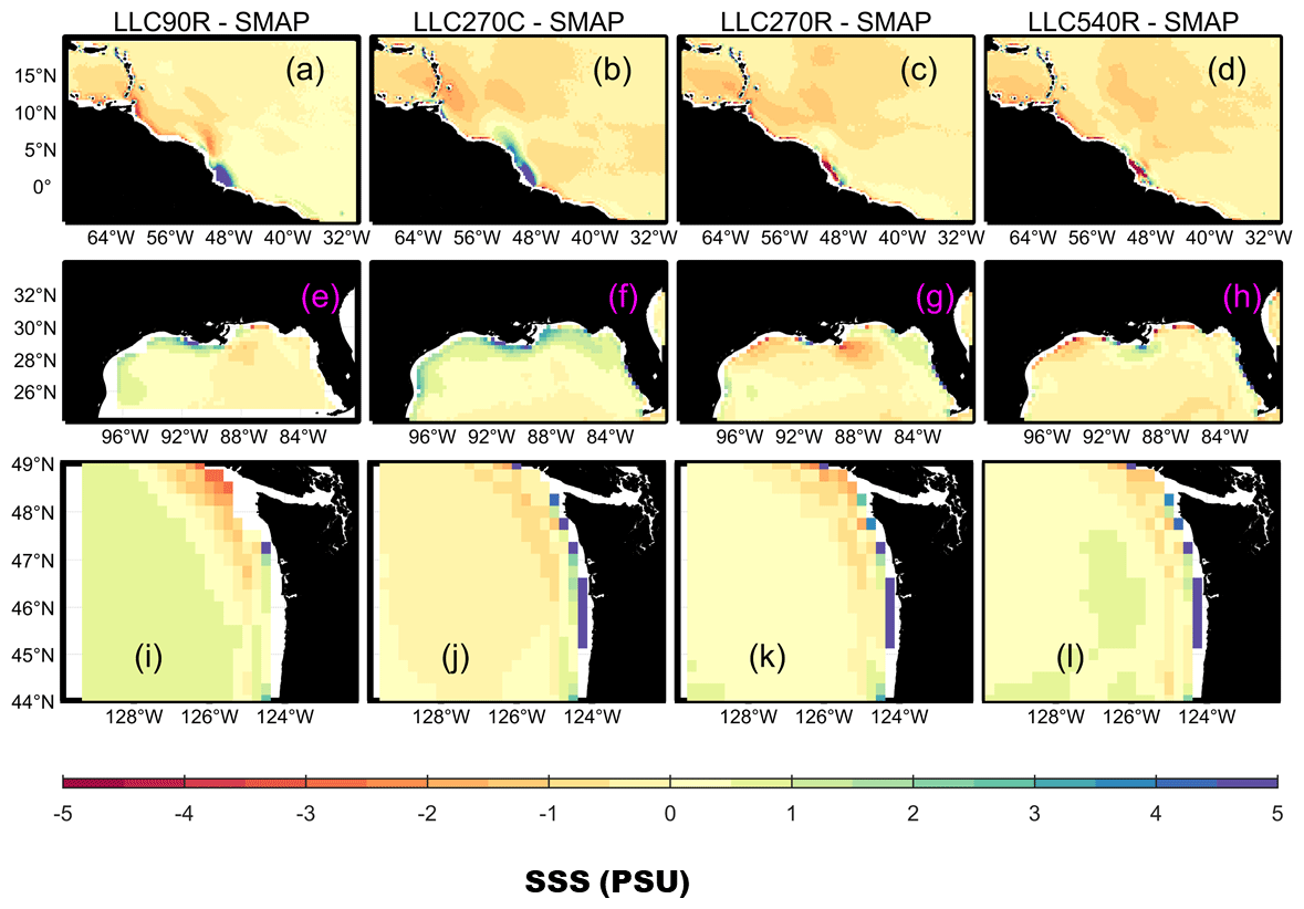
Figure 2Zoomed-in view of SSS difference between model experiments and SMAP observations for large (Amazon, a–d), medium (Mississippi, e–h), and small (Columbia, i–l) rivers.
Time series for all LLC simulations and SMAP, at these three river mouths, are shown in Fig. 3. As in Fig. 2, the bias decreases when daily, point-source river forcing is used and as the horizontal grid resolution increases. Additionally, We found the 2017 spring Amazon flood can be clearly seen when forced by diffusive daily JRA55DO (LLC270R_spread), but not in the diffusive climatological Fekete case (LLC270C). The Mississippi River mouth region is different from the Amazon in that the annual cycle of LLC270_spread is stronger than LLC270C. This is because the seasonality of the Mississippi–Atchafalaya river has been oversmoothed in the climatological Fekete. The Columbia river region is consistent with the Amazon in that there is an abnormal low salinity in 2017 in LLC270R_spread and LLC270R, which is because the peak discharge is successfully resolved by JRA55DO.
It is interesting to see the intermediate LLC270 resolution run is better than the high CS510 resolution run at the Amazon region. This is because the Stammer et al. (2004) runoff is smoother spatially and lacks seasonal variability compared to the Fekete et al. (2002) runoff in this region (Fig. S7). When using DPR forcing, the SSS differences associated with the river discharge interannual variability can be resolved as well. For example, the 2017 abnormally low SSS near the Amazon river mouth is associated with an extreme flooding event (Barichivich et al., 2018).

Figure 3Areally averaged SSS in the Amazon, Mississippi, and Columbia river mouth regions (see Fig. S3) with climatological diffusive and daily, point-source runoff forcing for SMAP (thick gray line) and experiments (thin colored lines) with varying horizontal grid resolution. The method used to characterize the river mouth region is described in Sect. 3.
Next, we quantify the difference in mean and variance between the SSS time series of LLC simulations and that of SMAP under daily JRA55DO runoff but using diffusive and point source methods for each (Fig. 4). We found the normalized bias with point source is lower than experiments with diffusive source. The normalized unbiased RMSD decrease is ignorable compared to the normalized bias decrease. This means the total normalized RMSD improvements are primarily due to the normalized bias decrease. We find that most unbiased RMSD remains negative when varying the runoff forcing from climatological to daily. This implies that the variance of LLC simulations remains lower than SMAP observations as the runoff forcing changes. The only exception is the Congo river, which is a near-Equator eastern boundary plume that freshwater transport may distinguish from others (Palma and Matano, 2017).
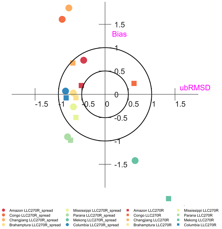
Figure 4SSS target diagram near the selected river mouths (see Fig. S3) for LLC270R_spread and LLC270R simulations.
We also examine the bias and variance on the target diagram for experiments with varying grid resolution but similar daily runoff forcing (Fig. 5). Our results show that the normalized bias decreases as the model resolution increases, which is consistent with the SSS reduction in Table 2 and relatively low Wskill in Table 3. The unbiased RMSD decreases slightly with the sign remaining negative as the model resolution increases. This occurs everywhere, except for the two largest rivers (AZ and CG) where the sign becomes positive for LLC540R, indicating that the model variance exceeds the SMAP variance when using the high-resolution grid. In summary, the comparison with synchronized SMAP shows that using daily runoff and finer horizontal grid resolution improves the representation of SSS variability but at a cost of increased SSS bias.
4.1 EOF analysis of SSS
We next investigate how model runoff improvements impact river plume properties such as plume area, volume, and freshwater thickness, since we are interested in how the widely used general ECCOv4 (forced by Fekete runoff)) will be different from the new DPR implementation. We limited our next discussion to LLC#C/R cases only (experiments 1, 2, 3, 4, and 7). We first evaluate the plume SSS signature and dynamics through EOFs; the mean is removed before the EOF analysis. The first and second mode of AZ, MR, and CO using the same grid resolution but different runoff forcing is shown in Figs. 6 and S4. The spatial pattern reveals the salinity anomaly caused by the runoff, while the PC time series shows the timing. A single value in spatial pattern or PC time series does not have a clear physical meaning, but together they reveal how much salinity deviates from the mean. The PC time series for experiments with DPR forcing clearly shows similar seasonal cycles, albeit with larger amplitudes and interannual variability.
For the AZ region, the LLC270R and LLC270C spatial patterns are similar for the first and second mode. The first mode accounts for 59 % (72 %) of the total variance in LLC270R (LLC270C). The spatial pattern reveals the presence of a low-salinity tongue; this is located in a narrow band along the northeastern South American coast from February–June, which is associated with the large river discharge and the northward-flowing Brazil Current. The second mode of LLC270R (LLC270C) accounts for 33 % (23 %) of the total variance. The spatial pattern shows that the plume-like features extend northwestward to the Caribbean Sea and Central Equatorial Atlantic Ocean from May–September. This pattern is driven by Ekman currents associated with northeasterly wind stress, and the transport to the Central Equator is due to the North Equatorial Counter Current (NECC; Lentz 1995a, b).
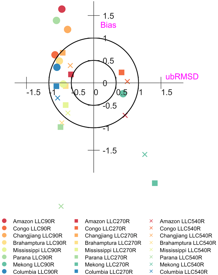
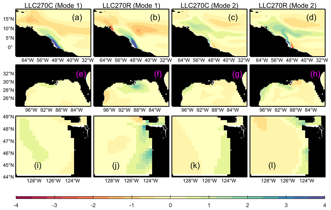
Figure 6First and second EOF spatial patterns from the LLC270C and LLC270R simulations for the Amazon, Mississippi, and Columbia rivers. The corresponding PC time series are normalized by the standard deviation and multiplied back to the spatial mode.
For the MR region, the first and second mode of LLC270R (LLC270C) explains 53 % (66 %) and 29 % (18 %) of the total variance, respectively. The spatial pattern of the first mode is generally similar. There is a bulge-like plume feature that occupies a region near the MR mouth with a southeast extension to the central Gulf of Mexico from May–October (Fig. S4), while the freshwater signal in the vicinity of the southeast MR mouth is stronger in LLC270R. The extension of low-salinity waters is due to the upwelling of favorable winds (southwesterly) from late spring to summer, which transport the MR freshwater offshore (Walker, 1996).
The first and second mode explains 63 % (56 %) and 29 % (33 %) of the variability at the CO region in LLC270C (LLC270R), respectively. It has been previously recognized that the CO plume exhibits seasonal variability forced by wind and freshwater discharge (García Berdeal et al., 2002). During winter, Ekman transport resulting from the northward winds constrains the plume against the Washington coast. Downwelling-favorable wind stresses strengthen the anti-cyclonic rotation of the river plume, resulting in a coastally attached winter plume. In contrast, prevailing southward wind stress results in offshore Ekman transport; this advects the plume offshore, where it is influenced by the California Current over long timescales and subsequently veers southward and offshore (Banas et al., 2009). This seasonal pattern is shown in the first LLC270R mode and second LLC270C mode.
The first and second EOF modes for AZ, MR, and CO with daily runoff forcing in coarse (LLC90R) and fine (LLC540R) grid resolution are shown in Figs. 7 and S5. The plume-like features and associated dynamics are similar to LLC270 in both runs. Additionally, the higher-resolution LLC540R resolves fine-scale plume structure for a number of major rivers, which was previously revealed by satellite observations, regional simulations, or neural network methods (e.g., meanders and rings of the AZ plume due to the NBC retroflection; Molleri et al., 2010); “horseshoe” patterns of the MR plume associated with Texas floods (Fournier et al., 2016b); and the bidirectional CO plume during variable summer wind patterns (Liu et al., 2009). Overall, EOF SSS analysis shows that general plume pattern and dynamics are grid independent; however, fine-scale plume structures are only resolved by high-resolution simulations.
4.2 Plume area, volume, and freshwater thickness
We first calculated the plume area using a salinity threshold from 28 to 36 PSU. The 3-year-average plume area for AZ, MR, and CO river region for different LLC configurations are present in Fig. 8. Under either the climatological diffusive or DPR river forcing, we could clearly see the plume area increase when model resolution increased from 1∘ to ∘ for all regions. However, when model resolution was increased to ∘, the plume area further increase can only be clearly seen in the Mississippi River region. To highlight the seasonal and interannual variability at the given threshold, we also show the plume area and volume within SA=30 PSU under the climatological and daily runoff forcing at the coarse, intermediate, and high-resolution runs (Figs. S6, 9). Figure 9 presents a time series of freshwater volume within the given salinity during this period. There is a stronger interannual variability when using DPR, along with larger plume area and volume during flood years. The MR and CO plume area and volume cannot be explicitly resolved at the SA=30 threshold when using the climatological and runoff forcing since river runoff has been distributed over broad spatial grids and surface salinity decrease is small. For the AZ region, the averaged plume area (volume) approaches 6 × 10⁴ km2 (7 × 10² km3) in LLC270C, whereas it is only about 3×10⁴ km2 (5 × 10² km3) in LLC90C. In contrast, the MR and CO plume area (volume) is easily recognized when using DPR forcing. The AZ plume increases as the grid resolution increases, reaching 10, 13, and 17 × 104 km2 in LLC90R, LLC270R, and LLC540R, respectively. The freshwater volume in coarse-, intermediate-, and high-resolution runs is comparable, with values of ∼ 1.5–2×10² km3. The plume area and volume in the MR region is more sensitive to the model grid resolution than AZ and CO. The LLC540R plume area is∼ 3–4 times higher than LLC270R, while LLC270R is ∼ 6–7 times higher than LLC90R. For the CO region, the plume area when using DPR forcing is similar between intermediate- and fine-resolution experiments, with the area in LLC270R and LLC540R increasing to ∼ 1 × 10⁵ km2 during the 2015 flood year. In contrast, LLC540R maintains a larger plume volume than the intermediate-resolution run.
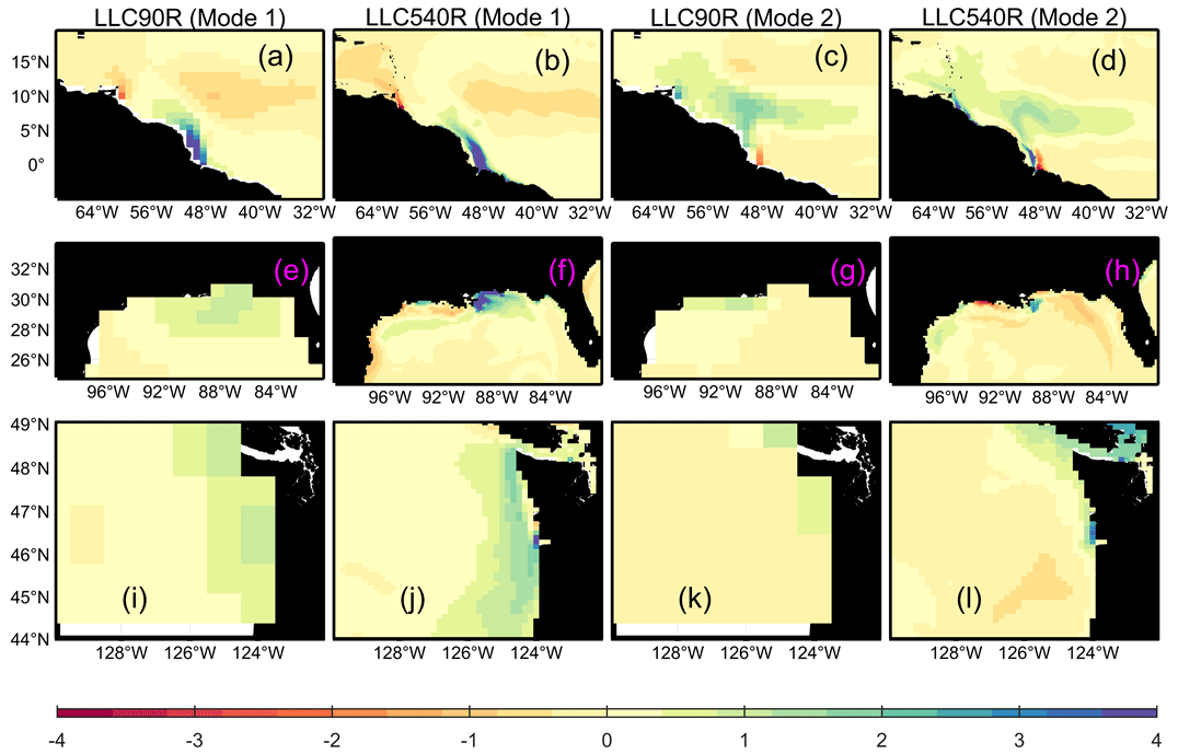
Figure 7Same as Fig. 6 but for the LLC90R and LLC540R simulations. The corresponding PC time series are normalized by the standard deviation and multiplied back to the spatial mode shown in Fig. S5.
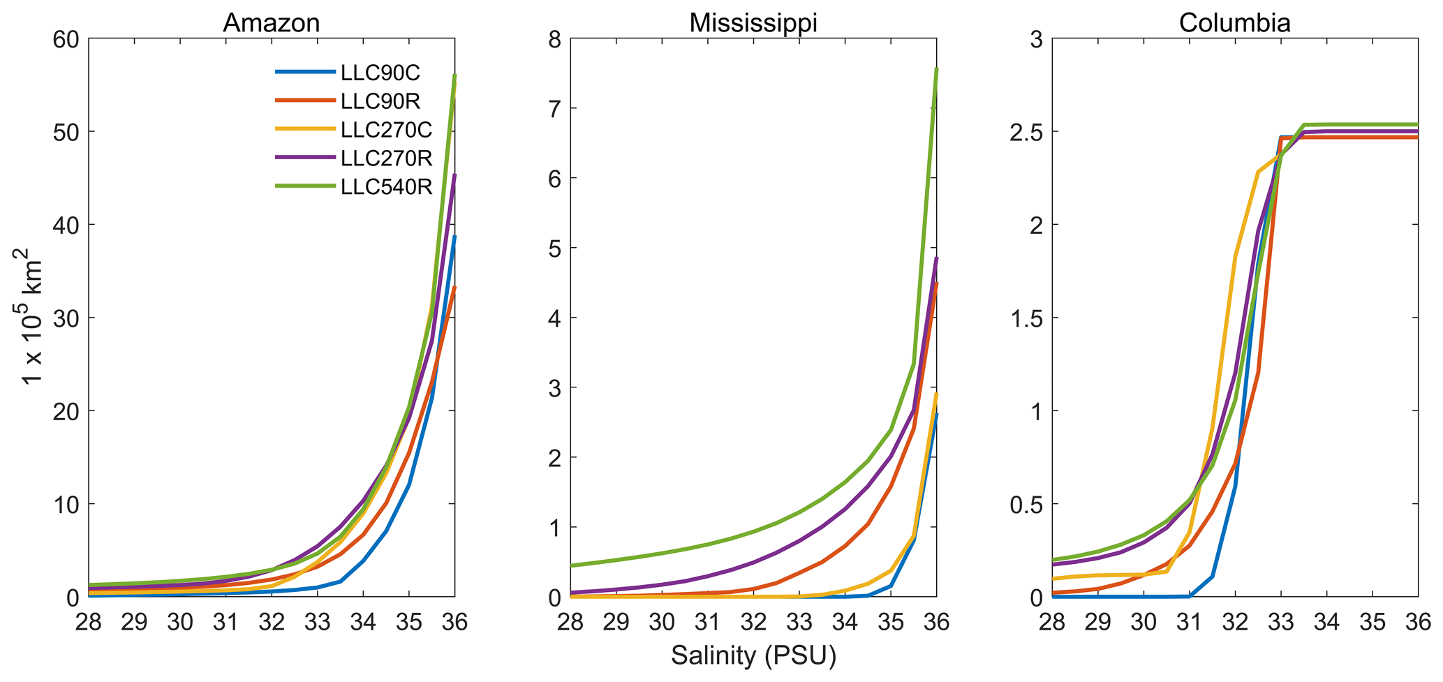
Figure 82015–2017 averaged plume area at salinity threshold SA from 28 to 36 for the Amazon, Mississippi, and Columbia River regions.
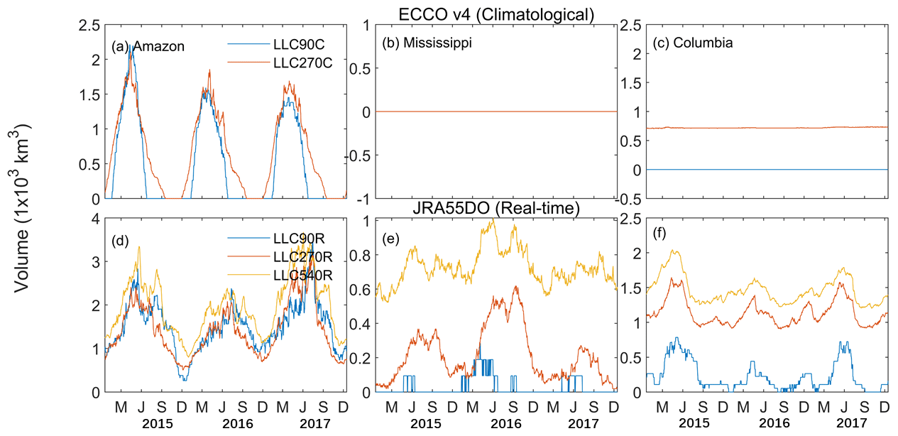
Figure 9Freshwater volume within 30 PSU for the Amazon, Mississippi, and Columbia river regions for various experiments; reference salinity is 36 PSU.
The sensitivity of plume area and volume to runoff forcing and grid resolution reflects the experiment's ability to resolve the horizontal advection and downward mixing of riverine freshwater. This can be partially reflected in the freshwater thickness calculation, which is shown in Fig. 10. For the intermediate-resolution experiments, the maximum freshwater thickness δfw is over 10, 5, and 4 m near the AZ, MR, and CO river mouths when using DPR, as opposed to 4, 2, and 2 m when using climatological runoff. Additionally, the freshwater thickness in experiments with DPR but different grid resolutions (LLC270R and LLC540R) demonstrates that a coherent plume rotates and responds to external wind and background flows; this coastal plume structure is largely absent in the coarser LLC90R. The coarse-resolution experiment exhibits a more diffuse response, with low salinity near MR and CO river mouths. Note that the runoff forcing is identical between LLC90R, LLC270R, and LLC540R experiments, and differences in plume area, volume, and freshwater thickness are due to model resolution alone. The freshwater flux in the higher resolution experiments can result in larger inflow velocities, a stronger baroclinic response, and consequently a more vigorous coastal plume. The plume area and volume in the MR region is more sensitive to grid resolution – this possibly results from the representation of shelf bathymetry. The Texas–Louisiana shelf is wider and shoals more gradually from the coastline compared to the northern Brazilian shelf (AZ) and Washington shelf (CO). When adding the same amount of freshwater in shallow water regions, high-resolution experiments generate a larger pressure gradient force than the intermediate resolution, which drive a stronger baroclinic effect and elevate coastal currents. The alongshore currents can advect the MR Plume water downcoast, enlarging the plume area. Besides, the plume waters may be entrained downward by strong sub-grid vertical mixing and adjustment, e.g., meso-scale eddies, when flowing offshore to the open ocean as the horizontal resolution increases from intermediate to high. The eddies in the high-resolution run at AZ and CR may break up the plumes, shrinking the area compared to the low-to-intermediate-resolution run (Fig. S6).
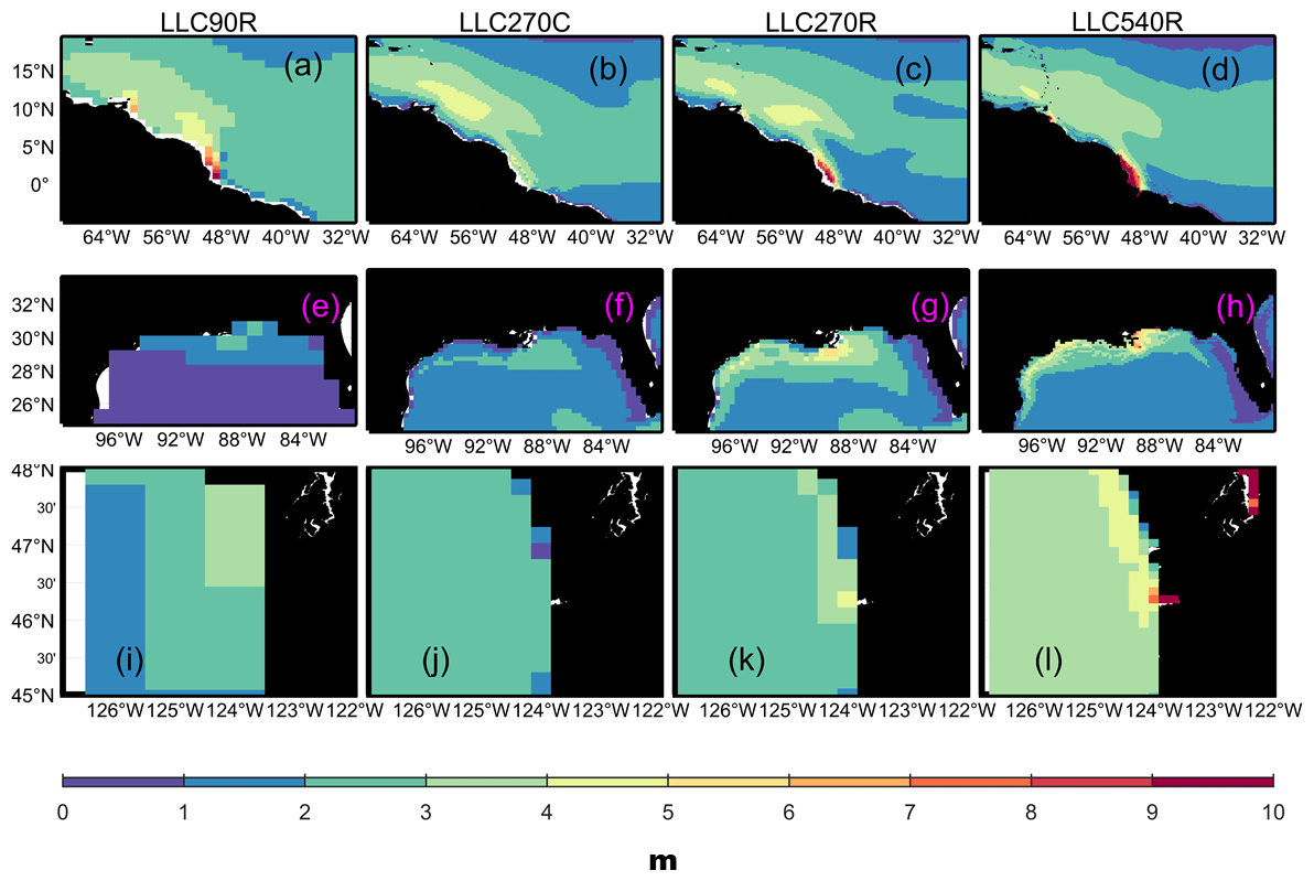
Figure 10Freshwater thickness for the Amazon, Mississippi, and Columbia river regions in LLC90R, LLC270C, LLC270R, and LLC540R experiments.
4.3 Impact on ocean properties associated with SSS
In this section, we examine the sensitivity of stratification and mixed layer depth (MLD) between different experiments. Figure 11 shows 3-year averaged vertical profiles of salinity, temperature, and vertical density gradient (ρ is the potential density) near the AZ (a–c), MR (d–f), and CO (g–i) river mouths, respectively. The profiles are averaged over the horizontal regions shown in Fig. S3. The vertical density gradient is an important indicator of stratification strength. The salinity differences between climatological (LLC90/270C) and DPR forcing (LLC90/270R) are large near the surface and diminish with increasing depth. The temperature difference when using the two types of runoff forcing is insignificant, demonstrating that the stratification is primarily determined by salinity and the addition of freshwater. Additionally, DPR forcing greatly increases subsurface stratification, which implies a decrease in vertical mixing.
Figure 11 also shows sensitivity of upper-ocean stratification to various model grid resolutions. The profiles show a significant decrease in salinity from the surface to 50 m depth as the resolution increases, which impacts the stratification (panels c, f, and i). We note that the vertical density gradient has a subsurface maximum in the coarse- and intermediate-resolution run, while the high-resolution experiment has a surface maximum due to low-salinity water concentrated in the surface level. SST is highest in LL540R at AZ and MR, reflecting that heat is preserved at the surface due to the increase in subsurface stratification.
The sensitivity of stratification in the above analysis implies that the MLD can be altered by river forcing and grid resolution. We compare the MLD in the vicinity of AZ, MR, and CO during the simulation period in Fig. 12. The MLD in our calculation uses the threshold method, in which deeper levels are examined until one is found with density differing from that the near surface by more than 0.03 kg/m3 (de Boyer Montégut et al., 2004). This reflects the maximum depth of the boundary layer that is sustained by riverine freshwater. Interestingly, all experiments simulate the annual cycle of MLD. There was relatively shallow MLD from April to December, which corresponds to periods of high river discharge. The MLD in the DPR forcing and high-resolution scenario is shallower than the climatological, low-resolution scenario, which is consistent with vertical salinity and stratification profiles shown in Fig. 11.

Figure 11Mean 3-year (2015–2017) salinity, potential temperature, and vertical density gradient () profiles.
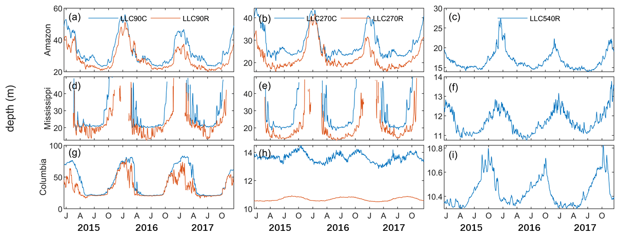
Figure 122015–2017 daily MLD, averaged in the vicinity of the Amazon River (a, b, c), Mississippi River (d, e, f), and Columbia River (g, h, i) mouth. MLD is computed based on de Boyer Montegut et al. (2004).
In this study, we investigate the model sensitivity of runoff forcing and grid resolution and type under the ECCO framework. We find that DPR greatly improves model representation of global rivers, with horizontal model resolution having a substantial control on SSS in the vicinity of river mouths. We observe no major changes in tropical and temperate river mouth SSS when using cube–sphere or LLC grid types when using the same river forcing. A comparison with synchronized SMAP observations shows that the use of DPR forcing and intermediate grid resolution can increase the model performance in simulating SSS in the vicinity of river mouths. However, further increasing model grid resolution from intermediate to high may result in an additional SSS bias towards fresher values.
Previous theoretical modeling studies have demonstrated that, in the absence of external forcing, large river plumes influenced by rotational effects tend to veer anticyclonically and form a bulge region near the river mouth as well as an along-shore downstream coastal current as Kelvin waves (Kourafalou et al., 1996; Yankovsky and Chapman, 1997). Additionally, idealized numerical simulations have revealed that river plume behavior is greatly impacted by external forcing. Chao (1988a, b) demonstrated that vertical mixing, bottom drag, and bottom slope greatly impact the spin-up, maintenance, and dissipation of river plumes. Fong and Geyer (2001) revealed that a surface-trapped river plume would thin and be advected offshore by cross-shore Ekman transport. Fong and Geyer (2002) suggested that the ambient current, which is in the same direction as the geostrophic coastal current, can augment plume transport. Our ECCO experiments are examining the above river plume dynamic theory globally with realistic topography and external atmospheric forcing. Our EOF analysis of SSS at the AZ, MR, and CO shelves show that the general spatial and temporal patterns plume related to river discharge, wind, and currents are independent of the grid resolutions and forcing formulations examined in this study, which are quite consistent with those previous studies. However, higher resolution and DPR forcing may be particularly important for resolving the fine-scale plume dynamics for small rivers. Using DPR forcing and increasing the model grid resolution from coarse to intermediate increases the river plume area and volume, while further increasing the model resolution from intermediate to high has mostly regional effects. Shallow and wide shelf regions, such as the Mississippi Delta, are more sensitive compared to AZ and CO. Nowadays, the increased computational power allows GODAS products such as ECCO to provide data at different resolutions, which supports regional scientific studies using a data analytical approach or offline method (e.g., the Lagrangian method; Meng et al., 2020; Liang et al., 2019). Our results suggest that how high-resolution products should be used depending on the spatiotemporal dynamics as well as geomorphology characteristic of the studied region itself.
We also found that using DPR forcing and increasing the model grid resolution can stabilize the water column at the subsurface and shoal the MLD. This may have significant implications for biogeochemical cycles and air–sea exchange in coastal zones. From the biogeochemistry perspective, freshwater introduced by the river increase shelf stratification, preventing the reoxygenation of bottom waters and thus may generate large hypoxic regions (Fennel et al., 2013; Feng et al., 2019). From the air–sea interaction perspective, on one hand, SST can trigger deep atmospheric convection and strong rainfall. On the other hand, strong near-surface stratification may inhibit cooling and intensify tropical cyclones (Cione and Uhlhorn, 2003; Neetu et al., 2012; Rao and Sivakumar, 2003; Sengupta et al., 2008; Vialard and Delecluse, 1998; Vinaychandran et al., 2002). We envision that future work investigating river impacts on ocean–atmosphere and Earth system dynamics could be accomplished by coupling our improved ECCO simulations with an atmospheric general circulation model (AGCM).
In the state-of-the-art OGCMs, ESMs, and most GODAS products, river runoff is incorporated into coarse-resolution grids as augmented precipitation. Climatological runoff forcing is often used in conjunction with artificial spreading, along with a virtual salt flux scheme. Tseng et al. (2016) examined model sensitivity to the spreading radius, turbulent mixing parameterization, reference salinity, and vertical distribution of riverine freshwater on 1∘ resolution in the Community Earth System Model (CESM). For all factors examined, they found that the model results are most sensitive to the spreading radius, which substantiates the importance of our finding that the associated plume properties, including the area and hence the SSS near river mouths, exhibit strong responses when switching the runoff flux from diffusive climatological to daily point source.
The present state-of-the-art regional-scale estuarine models can simulate estuarine hydrodynamics and biogeochemical processes in a robust manner. The inlet approach, which defines a rectangular breach in coastal land cells with uniform density and discharge, is widely used (Herzfeld, 2015; Garvine, 2001). An additional barotropic pressure term may be added to account for pressure gradients induced by the freshwater plume (Schiller and Kourafalou, 2011). The inlet approach has also been used in global z-coordinate models by injecting freshwater in multiple vertical grid cells (Griffies et al., 2005). In our simulations, changes in sea level are redistributed over all vertical grid cells by the rescaled height vertical coordinate. This is similar to the inlet approach in the regional models, which add a mass or volume flux of freshwater to a breach in coastal land cells (Garvine, 1999). Herzfeld (2015) investigated the role of model resolution on plume response at the Great Barrier Reef (GBR) using the Regional Ocean Modeling System (ROMS). The study found that the plume veered left and followed a northward trajectory to Cape Bowling Green in a 1 km resolution model but not in a 4 km resolution model. Our findings are consistent with this result; plume properties in our intermediate-resolution simulations are more clearly detected than in the coarse-resolution simulations. In addition, our results expand on their findings by showing that the sensitivity of plume properties in high-resolution models are highly dependent on shelf bathymetry. Schiller and Kourafalou (2010) investigated the dynamics of large-scale river plumes in idealized numerical experiments using HYCOM to address how the development and structure of a buoyant plume is affected by the vertical and horizontal redistribution of river inflow and bottom topography. Their experiments show that a narrow inlet and flat bottom facilitate a larger right-turning plume bulge region compared to a wide inlet and sloped bottom (see their Fig. 8; Riv2c-f, Riv2c-s). This is complementary to our findings that the MR plume, located on the wide and shallow LA shelf, has a larger horizontal plume area compared to the AZ and CO plume when increasing the horizontal resolution from intermediate to high. However, their discussion was limited to an idealized, rectangular model domain without external forcing, while our model simulations provide a realistic application to natural river plume systems. The global application of the regional inlet representation of river forcing was also used by NOAA's Geophysical Fluid Dynamics Laboratory (GFDL) models (Griffies et al., 2005). An internal, pre-computed salinity source term was introduced into multiple vertical layers. However, river representation was done through VSF rather than through real mass or freshwater volume flux. Adding the real volume and mass of freshwater through multiple layers has been widely used in regional models like ROMS; it may be useful to adapt this technology into future ECCO simulations and compare the results with the current surface injection methods.
For the global ocean, river runoff is much smaller than the precipitation and evaporation flux; therefore, for most OGCMs, ESMs, and GODAS products it is parameterized. One of the most significant expected signatures of global warming is an acceleration of the terrestrial hydrological cycle (IPCC, 2021; Piecuch and Wadehra, 2020). Both can significantly affect the magnitude, distribution, and timing of global runoff, leading to extremes in the frequency and magnitude of floods and droughts. When considering issues related to water resource management under climate and land use and land cover change, a key question such as “how will coastal oceans be impacted from flood and drought events?” is challenging to answer (Fournier et al., 2019). In the future, high-resolution global-ocean circulation models with DPR forcing may help identify the primary forcing mechanisms (such as those from climate-driven extreme events) that drive spatiotemporal variability of large river plume systems just as skillfully as regional model setups.
Improved model representation of rivers may not be as important for global- or basin-scale hydrological cycles as precipitation and evaporation (Du and Zhang, 2015) but may be critical for the global carbon cycle (Friedlingstein et al., 2019; Resplandy et al., 2018). River delivers large amounts of anthropogenic nutrients to the coastal zone (Seitzinger et al., 2005, 2010). The autochthonous production will transform inorganic nutrients to organic nutrients while sequestering atmospheric CO2. More importantly, rivers also deliver dissolved organic carbon (DOC) and particulate organic carbon (POC) to the coastal ocean, which can be remineralized and released as CO2 to the atmosphere. Until recently, most global-ocean biogeochemistry models omitted or poorly represented riverine point sources of nutrients and carbon. Lacroix et al. (2020) added yearly-constant riverine loads to the ocean surface layer on coarse-resolution (1.5∘) models and assessed that CO2 outgassing from river loads accounted for ∼ 10 % of the global ocean CO2 sink. We anticipate that the implementation of DPR forcing and higher-resolution grids in ESMs and the ECCO biogeochemical state estimates (ECCO-Darwin, Carroll et al., 2020) will help better resolve the global carbon budget (Friedlingstein et al., 2019).
LOAC development has historically had a low priority in OGCMs, ESMs, and GODAPs and exchange of freshwater between rivers/estuaries and the coastal ocean has been previously neglected. Our results demonstrate that the representation of runoff forcing in ECCO simulations is a major source of bias for coastal SSS. We believed our improvements of river runoff in ECCO will directly contribute to (i) the evaluation, understanding, and improvement of river-dominated coastal margins in global-ocean circulation models; (ii) investigation of mechanisms that drive seasonal and interannual variability in coastal plume processes; and (iii) bridging the gap between land–ocean interactions. These efforts will ultimately help to better resolve land–ocean–atmosphere processes and feedbacks in next-generation Earth system models.
The MITgcm and user manual are available from the project website: http://mitgcm.org/ (last access: 29 March 2021). The ECCOv4 setup can be found at http://wwwcvs.mitgcm.org/viewvc/MITgcm/MITgcm_contrib/llc_hires/ (Menemenlis, 2020a). The exact version of MITgcm, ECCOv4 configuration, and MATLAB routines to process the ECCOv4 output, generate the target model skill assessment diagram, and produce the paper figures are archived on Zenodo (https://doi.org/10.5281/zenodo.4106405, Feng, 2020). The SMAP observations can be downloaded from http://apdrc.soest.hawaii.edu/las/v6/dataset?catitem=2928 (Menemenlis, 2020b). The model forcing and simulated salinity fields at different resolutions are archived on Zenodo (https://doi.org/10.5281/zenodo.4095613, Zhang, 2020).
The supplement related to this article is available online at: https://doi.org/10.5194/gmd-14-1801-2021-supplement.
DM designed the experiments and HZ carried them out. YF, DM, and DC developed the model code and performed the simulations. YF prepared the paper with contributions from HX, DC, YD, and HW.
The authors declare that they have no conflict of interest.
This research has been supported by the CAS Pioneer Hundred Talents Program Startup Fund (grant no. Y9SL11001), the Southern Marine Science and Engineering Guangdong Laboratory (Guangzhou) (grant nos. GML2019ZD0303 and 2019BT02H594), the Guangdong Key Laboratory of Ocean Remote Sensing (grant no. 2017B030301005-LORS2002), the State Key Laboratory of Tropical Oceanography Independent Research Fund (grant no. LTOZZ2103), the Chinese Academy of Sciences (grant nos. XDA15020901 and 133244KYSB20190031), the Institution of South China Sea Ecology and Environmental Engineering (grant no. ISEE2018PY05), and the National Natural Science Foundation of China (grant nos. 41830538 and 42090042). Dimitris Menemenlis, Dustin Carroll, and Hong Zhang carried out research at the Jet Propulsion Laboratory, California Institute of Technology, under contract with NASA, with grants from biological diversity; physical oceanography; and modeling, analysis, and prediction programs.
This paper was edited by Qiang Wang and reviewed by two anonymous referees.
Adcroft, A. and Campin, J.-M.: Rescaled height coordinates for accurate representation of free-surface flows in ocean circulation models, Ocean Model., 7, 269–284, https://doi.org/10.1016/j.ocemod.2003.09.003, 2004.
Adcroft, A., Campin, J.-M. Hill, C., and Marshall, J.: Implementation of an Atmosphere–Ocean General Circulation Model on the Expanded Spherical Cube, Mon. Weather Rev., 132, 2845–2863, https://doi.org/10.1175/MWR2823.1, 2004.
Banas, N. S., MacCready, P., and Hickey, B. M.: The Columbia River plume as cross-shelf exporter and along-coast barrier, Cont. Shelf Res., 2, 292–301, https://doi.org/10.1016/j.csr.2008.03.011, 2009.
Barichivich, J., Gloor, E., Peylin, P., Brienen, R. J. W., Schöngart, J., Espinoza, J. C., and Pattnayak, K. C.: Recent intensification of Amazon flooding extremes driven by strengthened Walker circulation, Sci. Adv., 4, eaat8785, https://doi.org/10.1126/sciadv.aat8785, 2018.
Bentsen, M., Bethke, I., Debernard, J. B., Iversen, T., Kirkevåg, A., Seland, Ø., Drange, H., Roelandt, C., Seierstad, I. A., Hoose, C., and Kristjánsson, J. E.: The Norwegian Earth System Model, NorESM1-M – Part 1: Description and basic evaluation of the physical climate, Geosci. Model Dev., 6, 687–720, https://doi.org/10.5194/gmd-6-687-2013, 2013.
Bourgeois, T., Orr, J. C., Resplandy, L., Terhaar, J., Ethé, C., Gehlen, M., and Bopp, L.: Coastal-ocean uptake of anthropogenic carbon, Biogeosciences, 13, 4167–4185, https://doi.org/10.5194/bg-13-4167-2016, 2016.
Campin, J.-M., Marshall, J., and Ferreira, D.: Sea ice–ocean coupling using a rescaled vertical coordinate z∗, Ocean Model., 24, 1–14, https://doi.org/10.1016/j.ocemod.2008.05.005, 2008.
Carroll, D., Menemenlis, Adkins, J. F., Bowman, K. W., Brix, H., Dutkiewicz, S., Gierach, M. M., Hill, C., Jahn, O., Landschützer, P., Lauderdale, J. Liu, J. M., Naviaux, J. D., Manizza, M., Rödenbeck, C., Schimel, D. S., Van der Stocken, T., and Zhang, H.: The ECCO‐Darwin data‐assimilative global ocean biogeochemistry model: Estimates of seasonal to multidecadal surface ocean pCO2 and air‐sea CO2 flux, J. Adv. Model. Earth Sy., 12, e2019MS001888, https://doi.org/10.1029/2019MS001888, 2020.
Chao, S.-Y.: River-forced estuarine plumes, J. Phys. Oceanogr., 18, 72–88, https://doi.org/10.1175/1520-0485(1988)018<0072:RFEP>2.0.CO;2, 1988a.
Chao, S.-Y.: Wind-driven motion of estuarine plumes, J. Phys. Oceanogr., 18, 1144–1166, https://doi.org/10.1175/1520-0485(1988)018<1144:WDMOEP>2.0.CO;2; 1988b.
Cione, J. J. and Uhlhorn, E. W.: Sea surface temperature variability in hurricanes: Implications with respect to intensity change, Mon. Weather Rev., 131, 1783–1796, https://doi.org/10.1175//2562.1, 2003.
de Boyer Montégut, C., Madec, G., Fischer, A. S., Lazar, A., and Ludicone, D.: Mixed layer depth over the global ocean: An examination of profile data and a profile-based climatology, J. Geophys. Res.-Oceans, 109, C12003, https://doi.org/10.1029/2004jc002378, 2004.
Denamiel, C., Budgell, W. P., and Toumi, R.: The Congo River plume: Impact of the forcing on the far-field and near-field dynamics, J. Geophys. Res.-Oceans, 118, 964–989, https://doi.org/10.1002/jgrc.20062, 2013.
Du, Y. and Zhang, Y.: Satellite and Argo Observed Surface Salinity Variations in the Tropical Indian Ocean and Their Association with the Indian Ocean Dipole Mode, J. Climate, 28, 695–713, https://doi.org/10.1175/JCLI-D-14-00435.1, 2015.
Fekete, B. M., Vörösmarty, C. J., and Grabs, W.: High-resolution fields of global runoff combining observed river discharge and simulated water balances, Global Biogeochem. Cy., 16, 15-11–15-10, https://doi.org/10.1029/1999gb001254, 2002.
Feng, Y.: Improved representation of river runoff in ECCOv4 simulations: implementation, evaluation and impacts to coastal plume regions, Zenodo, https://doi.org/10.5281/zenodo.4106405, 2020.
Feng, Y., DiMarco, S. F., Balaguru, K., and Xue, H.: Seasonal and interannual variability of areal extent of the Gulf of Mexico hypoxia from a coupled physical-biogeochemical model: A new implication for management practice, J. Geophys. Res.-Biogeo., 124, 1939–1960, https://doi.org/10.1029/2018JG004745, 2019.
Fennel, K., Hu, J., Laurent, A., Marta-Almeida, M., and Hetland, R.: Sensitivity of hypoxia predictions for the northern Gulf of Mexico to sediment oxygen consumption and model nesting, J. Geophys. Res.-Oceans, 118, 990–1002, https://doi.org/10.1002/jgrc.20077, 2013.
Fennel, K., Alin, S., Barbero, L., Evans, W., Bourgeois, T., Cooley, S., Dunne, J., Feely, R. A., Hernandez-Ayon, J. M., Hu, X., Lohrenz, S., Muller-Karger, F., Najjar, R., Robbins, L., Shadwick, E., Siedlecki, S., Steiner, N., Sutton, A., Turk, D., Vlahos, P., and Wang, Z. A.: Carbon cycling in the North American coastal ocean: a synthesis, Biogeosciences, 16, 1281–1304, https://doi.org/10.5194/bg-16-1281-2019, 2019.
Fong, D. A. and Geyer, W. R.: Response of a river plume during an upwelling favorable wind event, J. Geophys. Res.-Oceans, 106, 1067–1084, https://doi.org/10.1029/2000jc900134, 2001.
Fong, D. A. and Geyer, W. R.: The Alongshore Transport of Freshwater in a Surface-Trapped River Plume, J. Phys. Oceanogr., 32, 957–972, https://doi.org/10.1175/1520-0485(2002)032<0957:TATOFI>2.0.CO;2, 2002.
Forget, G., Campin, J.-M., Heimbach, P., Hill, C. N., Ponte, R. M., and Wunsch, C.: ECCO version 4: an integrated framework for non-linear inverse modeling and global ocean state estimation, Geosci. Model Dev., 8, 3071–3104, https://doi.org/10.5194/gmd-8-3071-2015, 2015.
Fournier, S., Reager, J. T., Lee, T., Vazquez-Cuervo, J., David, C. H., and Gierach, M. M.: SMAP observes flooding from land to sea: The Texas event of 2015, Geophys. Res. Lett. 43, L070821, https://doi.org/10.1002/2016GL070821, 2016a.
Fournier, S., Lee, T., and Gierach, M. M., Seasonal and interannual variations of sea surface salinity associated with the Mississippi River plume observed by SMOS and Aquarius, Remote Sens. Environ., 180, 431–439, https://doi.org/10.1016/j.rse.2016.02.050, 2016b.
Fournier, S., Vialard, J., Lengaigne, M., Lee, T., Gierach, M. M., and Chaitanya, A. V. S.: Modulation of the Ganges-Brahmaputra river plume by the Indian Ocean dipole and eddies inferred from satellite observations, J. Geophys. Res.-Oceans, 122, 9591–9604, https://doi.org/10.1002/2017JC013333, 2017a.
Fournier, S., Vandemark, D., Gaultier, L., Lee, T., Jonsson, B., and Gierach, M. M.: Interannual variation in offshore advection of Amazon-Orinoco plume waters: Observations, forcing mechanisms, and impacts, J. Geophys. Res.-Oceans, 122, 8966–8982, https://doi.org/10.1002/2017JC013103, 2017b.
Fournier, S., Reager, J. T., Dzwonkowski, B., and Vazquez-Cuervo, J.: Statistical mapping of freshwater origin and fate signatures as land/ocean “regions of influence” in the Gulf of Mexico, J. Geophys. Res.-Oceans, 124, 4954–4973, https://doi.org/10.1029/2018JC014784, 2019.
Friedlingstein, P., Jones, M. W., O'Sullivan, M., Andrew, R. M., Hauck, J., Peters, G. P., Peters, W., Pongratz, J., Sitch, S., Le Quéré, C., Bakker, D. C. E., Canadell, J. G., Ciais, P., Jackson, R. B., Anthoni, P., Barbero, L., Bastos, A., Bastrikov, V., Becker, M., Bopp, L., Buitenhuis, E., Chandra, N., Chevallier, F., Chini, L. P., Currie, K. I., Feely, R. A., Gehlen, M., Gilfillan, D., Gkritzalis, T., Goll, D. S., Gruber, N., Gutekunst, S., Harris, I., Haverd, V., Houghton, R. A., Hurtt, G., Ilyina, T., Jain, A. K., Joetzjer, E., Kaplan, J. O., Kato, E., Klein Goldewijk, K., Korsbakken, J. I., Landschützer, P., Lauvset, S. K., Lefèvre, N., Lenton, A., Lienert, S., Lombardozzi, D., Marland, G., McGuire, P. C., Melton, J. R., Metzl, N., Munro, D. R., Nabel, J. E. M. S., Nakaoka, S.-I., Neill, C., Omar, A. M., Ono, T., Peregon, A., Pierrot, D., Poulter, B., Rehder, G., Resplandy, L., Robertson, E., Rödenbeck, C., Séférian, R., Schwinger, J., Smith, N., Tans, P. P., Tian, H., Tilbrook, B., Tubiello, F. N., van der Werf, G. R., Wiltshire, A. J., and Zaehle, S.: Global Carbon Budget 2019, Earth Syst. Sci. Data, 11, 1783–1838, https://doi.org/10.5194/essd-11-1783-2019, 2019.
García Berdeal, I., Hickey, B. M., and Kawase, M.: Influence of wind stress and ambient flow on a high discharge river plume, J. Geophys. Res.-Oceans, 107, 13-11–13-24, https://doi.org/10.1029/2001jc000932, 2002.
Garvine, R. W.: Penetration of buoyant coastal discharge onto the continental shelf: a numerical model experiment, J. Phys. Oceanogr., 29, 1892–1909, https://doi.org/10.1175/1520-0485(1999)029<1892:POBCDO>2.0.CO;2, 1999.
Garvine, R. W.: The impact of model configuration in studies of buoyant coastal discharge, J. Marine Resh., 59, 193–225, https://doi.org/10.1357/002224001762882637, 2001.
Gaspar, P., Grégoris, Y., and Lefevre, J.-M.: A simple eddy kinetic energy model for simulations of the oceanic vertical mixing: Tests at station Papa and long-term upper ocean study site, J. Geophys. Res.-Oceans, 95, 16179–16193, https://doi.org/10.1029/JC095iC09p16179, 1990.
Gierach, M. M., Vazquez-Cuervo, J., Lee, T., and Tsontos, V. M.: Aquarius and SMOS detect effects of an extreme Mississippi River flooding event in the Gulf of Mexico, Geophys. Res. Lett., 40, L50995, https://doi.org/10.1002/grl.50995, 2013.
Griffies, S. M., Gnanadesikan, A., Dixon, K. W., Dunne, J. P., Gerdes, R., Harrison, M. J., Rosati, A., Russell, J. L., Samuels, B. L., Spelman, M. J., Winton, M., and Zhang, R.: Formulation of an ocean model for global climate simulations, Ocean Sci., 1, 45–79, https://doi.org/10.5194/os-1-45-2005, 2005.
Halliwell, G. R.: Evaluation of vertical coordinate and vertical mixing algorithms in the HYbrid-Coordinate Ocean Model (HYCOM), Ocean Model., 7, 285–322, https://doi.org/10.1016/j.ocemod.2003.10.002, 2004.
Herzfeld, M.: Methods for freshwater riverine input into regional ocean models, Ocean Model., 90, 1–15, https://doi.org/10.1016/j.ocemod.2015.04.001, 2015.
Huang, R. X.: Real Freshwater Flux as a Natural Boundary Condition for the Salinity Balance and Thermohaline Circulation Forced by Evaporation and Precipitation, J. Phys. Oceanogr., 23, 2428–2446, https://doi.org/10.1175/1520-0485(1993)023<2428:RFFAAN>2.0.CO;2, 1993.
IPCC: Summary for Policymakers, in: Climate Change and Land: an IPCC special report on climate change, desertification, land degradation, sustainable land management, food security, and greenhouse gas fluxes in terrestrial ecosystems, edited by: Shukla, P. R., Skea, J., Calvo Buendia, E., Masson-Delmotte, V., Pörtner, H.-O., Roberts, D. C., Zhai, P., Slade, R., Connors, S., van Diemen, R., Ferrat, M., Haughey, E., Luz, S., Neogi, S., Pathak, M., Petzold, J., Portugal Pereira, J., Vyas, P., Huntley, E., Kissick, K., Belkacemi, M., and Malley, J., in press, 2021.
Jolliff, J. K., Kindle, J. C., Shulman, I., Penta, B., Friedrichs, M. A. M., Helber, R., and Arnone, R. A.: Summary diagrams for coupled hydrodynamic-ecosystem model skill assessment, J. Marine Syst., 76, 64–82, https://doi.org/10.1016/j.jmarsys.2008.05.014, 2009.
Kourafalou, V. H., Oey, L.-Y., Wang, J. D., and Lee, T. N.: The fate of river discharge on the continental shelf: 1. Modeling the river plume and the inner shelf coastal current, J. Geophys. Res., 101, 3415–3434, https://doi.org/10.1029/95JC03024, 1996.
Lacroix, F., Ilyina, T., and Hartmann, J.: Oceanic CO2 outgassing and biological production hotspots induced by pre-industrial river loads of nutrients and carbon in a global modeling approach, Biogeosciences, 17, 55–88, https://doi.org/10.5194/bg-17-55-2020, 2020.
Landschützer, P., Laruelle, G. G., Roobaert, A., and Regnier, P.: A uniform pCO2 climatology combining open and coastal oceans, Earth Syst. Sci. Data, 12, 2537–2553, https://doi.org/10.5194/essd-12-2537-2020, 2020.
Lentz, S. J.: The Amazon River plume during AMASSEDS: subtidal current variability and the importance of wind forcing, J. Geophys. Res.-Oceans, 100, 2377–2390, https://doi.org/10.1029/94JC00343, 1995a.
Lentz, S. J.: Seasonal variations in the horizontal structure of the Amazon plume inferred from historical hydrographic data, J. Geophys. Res.-Oceans, 100, 2391–2400, https://doi.org/10.1029/94JC01847, 1995b.
Liang, L., Xue, H., and Shu, Y.: The Indonesian throughflow and the circulation in the Banda Sea: A modeling study, J. Geophys. Res.-Oceans, 124, 3089–3106, https://doi.org/10.1029/2018JC014926, 2019.
Liao, X., Du, Y., Wang, T., Hu, S., Zhan, H., Liu, H., and Wu, G., High-Frequency Variations in Pearl River Plume Observed by Soil Moisture Active Passive Sea Surface Salinity, Remote Sensing, 12, 563, https://doi.org/10.3390/rs12030563, 2020.
Liu, Y., MacCready, P., and Hickey, B. M., Columbia River plume patterns in summer 2004 as revealed by a hindcast coastal ocean circulation model, Geophys. Res. Lett. 36, L02601, https://doi.org/10.1029/2008GL036447, 2009.
Marshall, J., Adcroft, A., Hill, C., Perelman, L., and Heisey, C.: A finite-volume, incompressible Navier Stokes model for studies of the ocean on parallel computers, J. Geophys. Res.-Oceans, 102, 5753–5766, https://doi.org/10.1029/96jc02775, 1997.
Mecklenburg, S., Drusch, M., Kerr, Y. H., Font, J., Martin-Neira, M., Delwart, S., and Crapolicchio, R.: ESA's soil moisture and ocean salinity mission: Mission performance and operations, IEEE T. Geosci. Remote, 50, 1354–1366, https://doi.org/10.1109/TGRS.2012.2187666, 2012.
Menemenlis, D.: ECCOv4 setup, available at: http://wwwcvs.mitgcm.org/viewvc/MITgcm/MITgcm_contrib/llc_hires/ (last access: 29 March 2021), 2020a.
Menemenlis, D.: SMAP observations, available at: http://apdrc.soest.hawaii.edu/las/v6/dataset?catitem=2928 (last access: 29 March 2021), 2020b.
Menemenlis, D., Hill, C. N., Adcroft, A. J., Campin, J.-M., Cheng, B., Ciotti, R. B., and Zhang, J.: NASA Supercomputer Improves Prospects for Ocean Climate Research, EOS Transactions AGU, 86, 89–96, https://doi.org/10.1029/2005EO090002, 2005.
Menemenlis, D., Campin, J.-M., Heimbach, P., Hill, C. N., Lee, T., Nguyen, A. T., and Zhang, H.: ECCO2: High Resolution Global Ocean and Sea Ice Data Synthesis, Mercator Ocean Quarterly Newsletter, 31, 13–21, 2008.
Meng, Z., Ning, L. Yuping G., and Yang, F.: Exchanges of surface plastic particles in the South China Sea through straits using Lagrangian method, J. Tropical Oceanogr., 39, 109–116, available at: http://journal15.magtechjournal.com/Jwk3_rdhyxb/article/2020/1009-5470/1009-5470-39-5-109.shtml (last access: 29 March 2021), 2020 (in Chinese with English abstract).
Molleri, G. S. F., Novo, E. M. L. M., and Kampel, M.: Space-time variability of the Amazon River plume based on satellite ocean color, Cont. Shelf Res., 30, 342–352, https://doi.org/10.1016/j.csr.2009.11.015, 2010.
Neetu, S., Lengaigne, M., Vincent, E. M., Vialard, J., Madec, G., Samson, G., and Durand, F.: Influence of upper-ocean stratification on tropical cyclones-induced surface cooling in the Bay of Bengal, J. Geophys. Res.-Oceans, 117, C12020, https://doi.org/10.1029/2012JC008433, 2012.
Palma, E. D. and Matano, R. P.: An idealized study of near equatorial river plumes, J. Geophys. Res.-Oceans, 122, 3599–3620, https://doi.org/10.1002/2016JC012554, 2017.
Piecuch, C. G. and Wadehra, R.: Dynamic sea level variability due to seasonal river discharge: A preliminary global ocean model study. Geophys. Res. Lett., 47, e2020GL086984, https://doi.org/10.1029/2020GL086984, 2020.
Rao, R. R. and Sivakumar, R.: Seasonal variability of the salt budget of the mixed layer and near-surface layer salinity structure of the tropical Indian Ocean from a new global ocean salinity climatology, J. Geophys. Res.-Oceans, 108, 3009, https://doi.org/10.1029/2001JC000907, 2003.
Resplandy, L., Keeling, R. F., Rödenbeck, C., Stephens, B. B., Khatiwala, S., Rodgers, K. B., Long, M. C., Bopp, L., and Tans, P. P.: Revision of global carbon fluxes based on a reassessment of oceanic and riverine carbon transport, Nat. Geosci., 11, 504–509, https://doi.org/10.1038/s41561-018-0151-3, 2018.
Roobaert, A., Laruelle, G. G. Landschützer, P., Gruber, N., Chou, L., and Regnier, P.: The Spatiotemporal Dynamics of the Sources and Sinks of CO2 in the Global Coastal Ocean, Global Biogeochem. Cy., 33, 1693–1714, https://doi.org/10.1029/2019GB006239, 2019.
Roullet, G. and Madec, G.: Salt conservation, free surface, and varying levels: A new formulation for ocean general circulation models, J. Geophys. Res.-Oceans, 105, 23927–23942, https://doi.org/10.1029/2000jc900089, 2000.
Santini, M. and Caporaso, L.: Evaluation of freshwater flow from rivers to the sea in CMIP5 simulations: Insights from the Congo River basin, J. Geophys. Res.-Atmos., 123, 10278–10300, https://doi.org/10.1029/2017JD027422, 2018.
Schiller, R. V. and Kourafalou, V. H.: Modeling river plume dynamics with the HYbrid Coordinate Ocean Model, Ocean Model., 33, 101–117, https://doi.org/10.1016/j.ocemod.2009.12.005, 2011.
Seitzinger, S. P., Harrison, J. A., Dumont, E., Beusen, A. H. W., and Bouwman, A. F.: Sources and delivery of carbon, nitrogen, and phosphorus to the coastal zone: An overview of Global Nutrient Export from Watersheds (NEWS) models and their application, Global Biogeochem. Cy., 19, GB4S01, https://doi.org/10.1029/2005GB002606, 2005.
Seitzinger, S. P., Mayorga, E., Bouwman, A. F., Kroeze, C., Beusen, A. H. W., Billen, G., Drecht, G. V., Dumont, E., Fekete, B. M., Garnier, J., and Harrison, J. A.: Global river nutrient export: A scenario analysis of past and future trends, Global Biogeochem. Cy., 24, GB0A08, https://doi.org/10.1029/2009GB003587, 2010.
Sengupta, D., Goddalehundi, B. R., and Anitha, D. S.: Cyclone-induced mixing does not cool SST in the post-monsoon North Bay of Bengal, Atmos. Sci. Lett., 9, 1–6, https://doi.org/10.1002/asl.162, 2008.
Stammer, D., Ueyoshi, K., Köhl, A., Large, W. G., Josey, S. A., and Wunsch, C.: Estimating air-sea fluxes of heat, freshwater, and momentum through global ocean data assimilation, J. Geophys. Res.-Oceans, 109, C05023, https://doi.org/10.1029/2003jc002082, 2004.
Su, Z., Wang, J., Klein, P., Thompson, A. F., and Menemenlis, D.: Ocean sub mesoscales as a key component of the global heat budget, Nat. Commun., 9, 775, https://doi.org/10.1038/s41467-018-02983-w, 2018.
Suzuki, T., Yamazaki, D., Tsujino, H., Komuro, Y., Nakano, H., and Urakawa, S.: A dataset of continental river discharge based on JRA-55 for use in a global ocean circulation model, J. Oceanogr., 74, 421–429, https://doi.org/10.1007/s10872-017-0458-5, 2018.
Timmermann, R., Danilov, S., Schröter, J., Böning, C., Sidorenko, D., and Rollenhagen, K.: Ocean circulation and sea ice distribution in a finite element global sea ice–ocean model, Ocean Model., 27, 114–129, https://doi.org/10.1016/j.ocemod.2008.10.009, 2009.
Tseng, Y.-H., Bryan, F. O., and Whitney, M. M.: Impacts of the representation of riverine freshwater input in the community earth system model, Ocean Model., 105, 71–86, https://doi.org/10.1016/j.ocemod.2016.08.002, 2016.
Tsujino, H., Urakawa, S., Nakano, H., Small, R. J., Kim, W. M., Yeager, S. G., Danabasoglu, G., Suzuki, T., Bamber, J. L., Bentsen, M., Böning, C. W., Bozec, A., Chassignet, E. P., Curchitser, E., Boeira Dias, F., Durack, P. J., Griffies, S. M., Harada, Y., Ilicak, M., Josey, S. A., Kobayashi, C., Kobayashi, S., Komuro, Y., Large, W. G., Sommer, J. L., Marsland, S. J., Masina, S., Scheinert, M., Tomita, H., Valdivieso, M., and Yamazaki, D.: JRA-55 based surface dataset for driving ocean–sea-ice models (JRA55-do), Ocean Model., 130, 79–139, https://doi.org/10.1016/j.ocemod.2018.07.002, 2018.
Vialard, J. and Delecluse, P.: An OGCM study for the TOGA decade. Part I: Role of salinity in the physics of the western Pacific fresh pool, J. Phys. Oceanogr., 28, 1071–1088, https://doi.org/10.1175/1520-0485(1998)028<1071:AOSFTT>2.0.CO;2, 1998.
Vinaychandran, P., Murty, V. S. N., and Ramesh Babu, V.: Observations of barrier layer formation in the Bay of Bengal during summer monsoon, J. Geophys. Res.-Oceans, 107, 8018, https://doi.org/10.1029/2001JC000831, 2002.
Volodin, E. M., Dianskii, N. A., and Gusev, A. V.: Simulating present-day climate with the INMCM4.0 coupled model of the atmospheric and oceanic general circulations, Izvestiya, Atmos. Ocean. Phys., 46, 414–431, https://doi.org/10.1134/S000143381004002X, 2010.
Walker, N. D.: Satellite assessment of Mississippi River plume variability: causes and predictability, Remote Sens. Environ., 58, 21–35, https://doi.org/10.1016/0034-4257(95)00259-6, 1996.
Ward, N. D., Megonigal, J. P., Bond-Lamberty, B., Bailey, V. L., Butman, D., Canuel, E. A., Diefenderfer, H., Ganju, N. K., Goñi, M. A., Graham, E. B., Hopkinson, C. S., Khangaonkar, T., Langley, J. A., McDowell, N. G., Myers-Pigg, A. N., Neumann, R. B., Osburn, C. L., Price, R. M., Rowland, J., Sengupta, A., Simard, M., Thornton, P. E., Tzortziou, M., Vargas, R., Weisenhorn, P. B., and Windham-Myers, L.: Representing the function and sensitivity of coastal interfaces in Earth system models, Nat. Commun., 11, 2458, https://doi.org/10.1038/s41467-020-16236-2, 2020.
Willmott, C. J.: On the validation of models, Phys. Geogr., 2, 184–194, https://doi.org/10.1080/02723646.1981.10642213, 1981.
Yankovsky, A. E. and Chapman D. C.: A Simple Theory for the Fate of Buoyant Coastal Discharges, J. Phys. Oceanogr., 27, 1386–1401, https://doi.org/10.1175/1520-0485(1997)027<1386:ASTFTF>2.0.CO;2, 1997.
Yueh, S. H., Tang, W., Fore, A. G., Neumann, G., Hayashi, A., Freedman, A., and Lagerloef, G. S. L-band passive and active microwave geophysical model functions of ocean surface winds and applications to Aquarius retrieval, IEEE T. Geosci. Remote, 51, 4619–4632, https://doi.org/10.1109/TGRS.2013.2266915, 2013.
Yueh, S. H., Tang, W., Fore, A., Hayashi, A., Song, Y. T., and Lagerloef, G.: Aquarius geophysical model function and combined active passive algorithm for ocean surface salinity and wind retrieval, J. Geophys. Res.-Oceans, 119, 5360–5379, https://doi.org/10.1002/2014JC009939, 2014.
Zhang, H.: MITgcm model setup and output for “Improved representation of river runoff in ECCO simulations: implementation, evaluation, and impacts to coastal plume regions” [Data set], Zenodo, https://doi.org/10.5281/zenodo.4095613, 2020.
Zhang, H., Menemenlis, D., and Fenty, G.: ECCO LLC270 ocean‐ice state estimate, available at: http://hdl.handle.net/1721.1/119821 (last access: 29 March 2021), 2018.