the Creative Commons Attribution 4.0 License.
the Creative Commons Attribution 4.0 License.
 | 31 Mar 2021
GO_3D_OBS: the multi-parameter benchmark geomodel for seismic imaging method assessment and next-generation 3D survey design (version 1.0)
Stéphane Operto
Detailed reconstruction of deep crustal targets by seismic methods remains a long-standing challenge. One key to address this challenge is the joint development of new seismic acquisition systems and leading-edge processing techniques. In marine environments, controlled-source seismic surveys at a regional scale are typically carried out with sparse arrays of ocean bottom seismometers (OBSs), which provide incomplete and down-sampled subsurface illumination. To assess and minimize the acquisition footprint in high-resolution imaging process such as full waveform inversion, realistic crustal-scale benchmark models are clearly required. The deficiency of such models prompts us to build one and release it freely to the geophysical community. Here, we introduce GO_3D_OBS – a 3D high-resolution geomodel representing a subduction zone, inspired by the geology of the Nankai Trough. The model integrates complex geological structures with a viscoelastic isotropic parameterization. It is defined in the form of a uniform Cartesian grid containing ∼33.6e9 degrees of freedom for a grid interval of 25 m. The size of the model raises significant high-performance computing challenges to tackle large-scale forward propagation simulations and related inverse problems. We describe the workflow designed to implement all the model ingredients including 2D structural segments, their projection into the third dimension, stochastic components, and physical parameterization. Various wavefield simulations that we present clearly reflect in the seismograms the structural complexity of the model and the footprint of different physical approximations. This benchmark model is intended to help to optimize the design of next-generation 3D academic surveys – in particular, but not only, long-offset OBS experiments – to mitigate the acquisition footprint during high-resolution imaging of the deep crust.
- Article
(27203 KB) - Full-text XML
- BibTeX
- EndNote


To make a step change in our understanding of the geodynamical processes that shape the earth's crust, we need to improve our ability to build 3D high-resolution multi-parameter models of geological targets at the regional scale. This deep target reconstruction is typically beyond the range of the streamer-based data acquisition due to the limited length of the streamer cable (∼6 km). To meet this challenge, it becomes crucial to design numerical models and related synthetic experiments further promoting a new generation of crustal-scale seismic surveys. Along with the design of new acquisition settings, a quest for high-resolution reconstruction requires us to assess the feasibility of the leading-edge seismic imaging techniques and develop their necessary adaptations to the new acquisition specifications. In the context of this study, by seismic imaging we understand the broad range of procedures for estimating the earth's rock parameters from seismic data – including travel time tomography, migration-based velocity analysis, ray-based and reverse-time pre-stack depth migration, and full waveform inversion. Among them, velocity reconstruction methods including first-arrival travel time tomography (FAT) (Zelt and Barton, 1998), reflection tomography (Bishop et al., 1985; Farra and Madariaga, 1988), joint refraction and reflection tomography (Korenaga et al., 2000; Meléndez et al., 2015), slope tomography (Billette et al., 1998; Lambaré, 2008; Tavakoli F. et al., 2017, 2019; Sambolian et al., 2019), wavefront tomography (Bauer et al., 2017), finite-frequency travel time tomography (Mercerat and Nolet, 2013; Zelt and Chen, 2016), wave equation tomography (Luo and Schuster, 1991; Tong et al., 2014), and full waveform inversion (FWI) (Tarantola, 1984; Mora, 1988; Pratt et al., 1996) shall be examined against large-scale numerical problems and complex synthetic datasets generated in an ultra-long-offset configuration. Combining these methods with the up-to-date seismic acquisition techniques available nowadays should allow for regional-scale seismic imaging of continental margins at sub-wavelength spatial resolution (typically few hundred metres) (Morgan et al., 2013).
During the last decades, a vast majority of deep-crustal seismic experiments carried out in academia were performed in two dimensions (namely, along profiles), mainly due to the financial cost of such experiments and the lack of suitable equipments. They often combine a short-spread towed-streamer acquisition with sparse 4C (four-component) OBS (ocean bottom seismometer) deployments. The data recorded by these two types of acquisition conceptually provide complementary information on the subsurface, which is processed with different imaging techniques (Górszczyk et al., 2019). Streamer data are used for migration-based imaging of the reflectivity of the uppermost crust, while the OBS data are routinely utilized to build smooth P-wave velocity models of the crust by FAT. However, the rapidly increasing inaccuracy of the migration velocities with depth and the lack of aperture coverage provided by streamer acquisition generate poor-quality migrated sections at depths exceeding the streamer length. On the other hand, the low resolution of the velocity models built by FAT prevents an in-depth geological interpretation of complex media. Put together, these two pitfalls currently make the joint interpretation of migrated sections and tomographic velocity models quite illusory. Moreover, off-plane wavefield propagation makes the 2D acquisition geometry implicitly inaccurate, further increasing the uncertainty of the resulting images. The need for enhancement of this acquisition and processing paradigm is therefore obvious.
Regarding streamer acquisition, to date only a few 3D academic multi-streamer experiments have been conducted (Bangs et al., 2009; Marjanović et al., 2018; Lin et al., 2019). However, these experiments were performed with a small number of streamers and small spread (typically ∼6 km). The limited width of the receiver swath leads to narrow azimuth coverage and prevents the survey of a large area with a reasonable acquisition time, while the short length of the streamer limits the maximum depth of investigation as above mentioned. In contrast, the oil industry nowadays carries out 3D wide-azimuth streamer surveys with a swath of ∼1 km in width and streamers of up to 15 km in length arranged in a single or multi-vessel configuration. The long streamers and wide receiver swaths combined with shooting the lines in a race track mode would make the acquisition time of the crustal-scale surveys reasonable (Li et al., 2019) while at the same time increasing the penetration depth of the wavefield.
For stationary-receiver surveys, coarse 3D passive- or active-source OBS experiments have begun to emerge in academia (Morgan et al., 2016; Goncharov et al., 2016; Heath et al., 2019; Arai et al., 2019). Sparse areal OBS deployments provide the necessary flexibility to design long-offset acquisition geometries, such that energetic diving waves and post-critical reflections could sample the deepest targeted-structures (lower crust, Moho, upper mantle). While recent trends in exploration industry show intensive development toward seabed acquisitions carried out with large pools of autonomous nodes (Ni et al., 2019; Blanch et al., 2019), it creates the opportunity to adapt this development to academic regional experiments through a relaxation of the acquisition sampling. Indeed, industry-oriented surveys are often designed with the aim to apply the entire seismic imaging workflow to the recorded dataset (namely velocity analysis and migration). For this purpose, large pools of receivers are required to fulfil sampling criteria for high-frequency migration (Li et al., 2019). This requirement can be relaxed when aiming at the velocity reconstruction only using frequencies lower than 15 Hz (Mei et al., 2019).
In terms of imaging, processing of streamer data interlaces two tasks under a scale-separation assumption: reconstruction of the reflectivity by depth migration (from ray-based Kirchhoff migration to two-way wave equation reverse-time migration, RTM) and velocity model building by reflection or slope tomography. Stable velocity model building with those techniques can be performed down to a maximum depth of the order of the streamer length. In turns, reflectivity imaging by migration may be performed at greater depths if reliable deep velocity information is provided (e.g. from complementary OBS data) and the deep reflection are recorded with an acceptable signal-to-noise ratio. Higher-resolution velocity models can also be built from streamer data by FWI (Shipp and Singh, 2002; Qin and Singh, 2017) if the information carried out by diving waves is made usable after the re-datuming of the data on the seabed (Gras et al., 2019). As an alternative to classical FWI, a velocity model can be built by reflection waveform inversion (RWI), a reformulation of FWI where the reflectivity estimated by least-squares RTM is used as a secondary buried source to update the velocities along the reflection paths connecting the reflectors to the sources and receivers (Xu et al., 2012; Brossier et al., 2015; Zhou et al., 2015; Wu and Alkhalifah, 2015).
All these approaches have been designed to deal with the limited aperture illumination provided by short-spread streamer acquisition, which generates a null space between the low wavenumbers of the velocity macro-model and the high wavenumbers of the reflectivity image, hence justifying the explicit above-mentioned scale separation during seismic imaging (Claerbout, 1985; Jannane et al., 1989; Neves and Singh, 1996). Compared to streamer data, long-offset OBS data recorded by stationary-receiver surveys contain a wider aperture content and richer information about the deep crust and upper mantle. This information can be processed by travel time tomography and waveform inversion techniques – the former providing a kinematically accurate starting model for the latter (Kamei et al., 2012; Górszczyk et al., 2017). The term “long-offset data” refers to seismic data which record diving and refracted waves that undershoot the targeted structures. Under this condition, the angular illumination of the structure is sufficiently wide to build high-resolution crustal models by FWI. Therefore, FWI should be regarded as the method of choice for long-offset stationary-receiver data.
FWI is a brute-force nonlinear waveform matching procedure which allows for building broadband subsurface models – provided that the structure is illuminated by a variety of waves propagating from the transmission to the reflection regime (Sirgue and Pratt, 2004). Diving waves, pre- and post-critical reflections, diffractions, etc., have the potential to generate a wide range of scattering from the targeted structure and therefore can probe this structure with various wavenumber vectors (Fig. 1a). By a broadband model we understand a low-pass-filtered version of the true earth, where the local cut-off wavenumbers in each x, y, and z spatial direction are controlled by the local wavelength and the scattering, dip, and azimuth angles sampled by the acquisition (Fig. 1b). This means that the resolution obtained with FWI depends not only on the frequency bandwidth of the data but also on the aperture with which the wave interacts with the heterogeneities to be reconstructed (Operto et al., 2015). Fulfilling this wide-angular illumination specification is the first fundamental methodological issue for successful application of FWI to OBS data. Indeed, this wide-aperture illumination provided by long-offset acquisition is achieved at the expense of the receiver sampling, whose imprint in the model reconstruction should be assessed. When a limited pool of instruments is available, the down-sampling of the acquisition is directly mapped into the down-sampling of the subsurface wavenumbers, leading to spatial aliasing or wraparound in the spatial domain. A second fundamental methodological issue is therefore to mitigate the aliasing artefacts by reliable compressive sensing techniques and sparsity-promoting regularization during FWI (Herrmann, 2010; Aghamiry et al., 2019b). The third main issue is related to the well-known nonlinearity of the FWI associated with cycle skipping (e.g. Virieux and Operto, 2009). When a classical form of the least-squares misfit function is used (namely, the least-squares norm of the difference between the simulated and the recorded data), FWI can remain stuck in a local minimum when the initial model does not allow one to predict travel times with errors smaller than half a period. The cycle-skipping condition is indeed increasingly difficult to satisfy when the number of propagated wavelengths increases as in the case of ultra-long-offset regional surveys (Pratt, 2008). This issue can be addressed by developing kinematically accurate starting velocity models by travel time tomography (Górszczyk et al., 2017); by breaking down FWI into several data-driven multiscale steps according to frequency, travel time, and offset continuation strategies (Kamei et al., 2013; Górszczyk et al., 2017); by designing more robust distances in FWI (Warner and Guasch, 2016; Métivier et al., 2018); or by extending the linear regime of FWI by the relaxation of the physical constraints (van Leeuwen and Herrmann, 2013; Aghamiry et al., 2019a). The final key challenge is related to the computational burden resulting from wave simulation in huge computational domains. The only panacea here can be given through a development of efficient, massively parallel modelling, inversion, and optimization schemes tailored to the high-performance-computing architecture available nowadays.
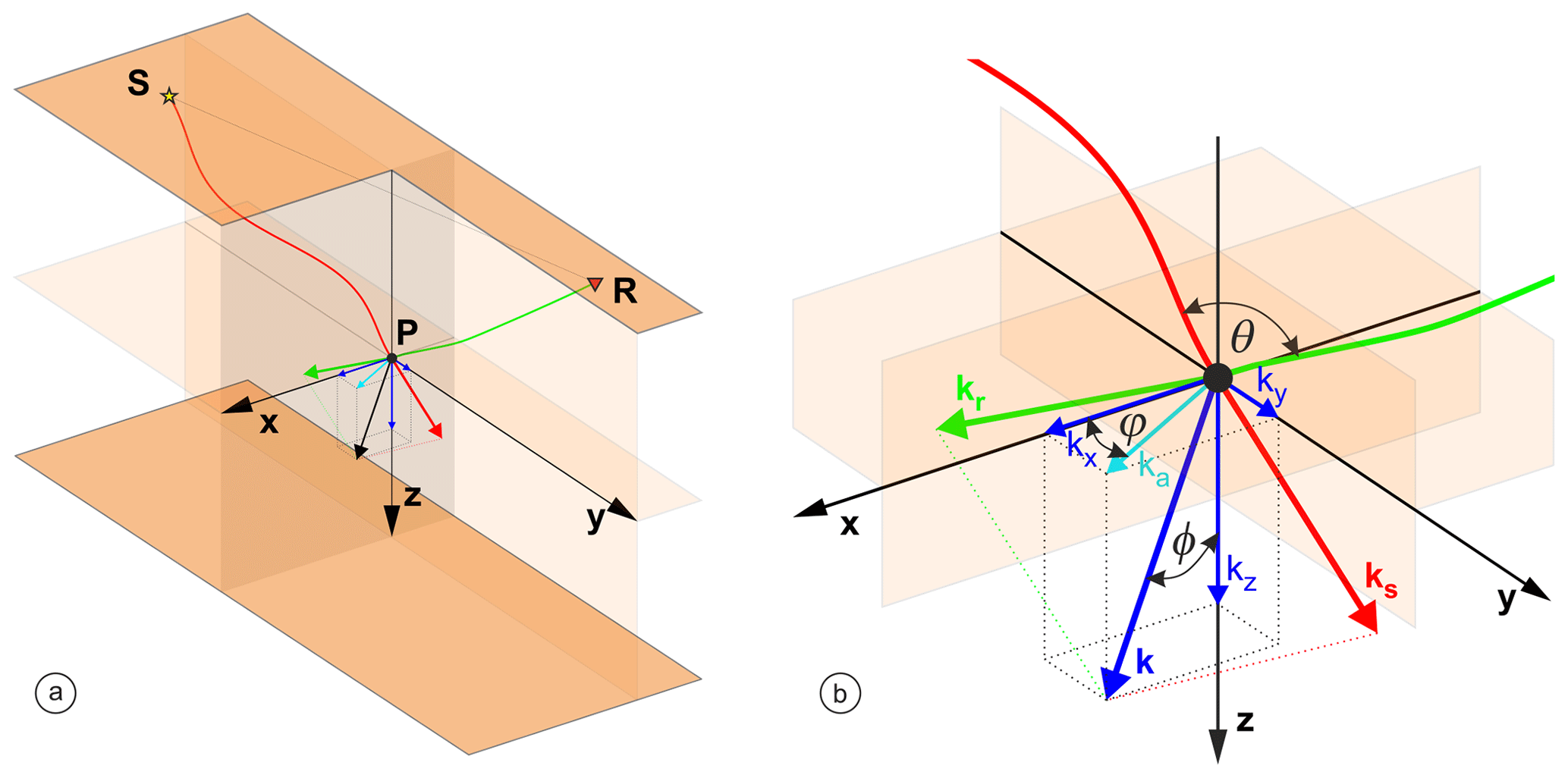
Figure 1(a) Sketch of the single source/receiver () acquisition and the 3D wavenumber vector k mapped by FWI at the scattering point P. (b) Zoom on (a). Local wavenumber vector k is a sum of the ks and kr vectors associated with the ray paths emerging from the source S and receiver R creating the scattering angle θ at the scattering point P. Dip and azimuth of the wavenumber vector k are defined by the ϕ and φ angles. The modulus of k is given by , where λ denotes the local wavelength (Miller et al., 1987; Wu and Toksöz, 1987). The range of k mapped at each point P by the acquisition gives the resolution with which the subsurface is reconstructed by FWI.
As reviewed above, advanced deep-crustal seismic imaging raises different frontier methodological issues in terms of acquisition design, inverse problem theory and high-performance computing. Addressing these challenges can be done by establishing a geologically meaningful 3D marine regional model amenable to exploring the pros and cons of different acquisition geometries, wave propagation requirements, and processing techniques. Indeed, most of the geomodels in the imaging community have been designed to fit the specifications of the exploration scale (Marmousil Versteeg, 1994; SEG/EAGE salt and overthrust, Aminzadeh et al., 1997; 2004 BP salt model, Billette and Brandsberg-Dahl, 2004; SEAM models, Pangman, 2007), while available crustal-scale geomodels are rather smooth or lack well defined structures and are 2D (e.g. 2D CCSS blind-test model, Hole et al., 2005; Brenders and Pratt, 2007b, a). In contrast our proposed geomodel shall incorporate a representative sample of three-dimensional geological structures detectable at the seismic scale (faults, sediment cover, main structural units, and discontinuities) and a multi-parameter physical definition of those structures (Wellmann and Caumon, 2018). A suitable natural environment to fulfil such specifications is provided by subduction zones. Indeed, the complex geological architecture of these margins warrants the variety of structures characterized by distinct physical parameters. Moreover, convergent margins still crystallize in many studies on the role of structural factors (sea mounts, subduction channel, etc.) and fluids on the rupture process of megathrust earthquakes (Kodaira et al., 2002). Therefore, capitalizing on our experiences from the previous imaging studies in the region of the eastern Nankai Trough (Dessa et al., 2004; Operto et al., 2006; Górszczyk et al., 2017, 2019) and combining them with the diverse geological features – typically interpreted in the convergent margins around the world – we aim at building a regional synthetic model of the subduction zone.
The proposed geomodel is intended to serve as an experimental setting for various imaging approaches with a special emphasize on multi-parameter waveform inversion techniques. For this purpose, the size of geological features we introduce shall be detectable by seismic waves and span tens of kilometres (major structural units building mantle, crust, volcanic ridges, etc.) to tens of metres – namely to the order of the smallest seismic wavelengths (sedimentary cover, subducting channel, thrusts, and faults, etc.). The structural complexity of the model is complemented by a broad range of physical parameters. Our approach incorporates deterministic, stochastic and empirical components at various stages of the model building. The deterministic components cover the shape of the main geological units, as well as their projection into the third dimension. The stochastic components include small-scale perturbations and random structure warping – introducing further spatial variation (Holliger et al., 1993; Goff and Holliger, 2003; Hale, 2013). The empirical components combine the physical parameterization of the model – Vp, Vs, ρ (density), Qp, Qs – namely the magnitude and relations between the subsequent parameters (Brocher, 2005; Wiggens et al., 1978; Zhang and Stewart, 2008). Such a combination of structural and parametric variability is reflected by the anatomy of the seismic wavefield, making it suitable to benchmark different imaging approaches. We obtain the 3D cube through the projection of the initial 2D inline profile towards the strike direction of subduction, leading to realistic changes in the geological structure along the crossline extension of the model. The dimension of the final model equals leading to ∼ 33.6e9 degrees of freedom in a Cartesian grid with a 25 m grid step. Therefore, away from the challenges related to the reconstruction of the geologically complex setting, the model imposes a significant computational burden in terms of seismic wavefield modelling. The large size of the computing domain can further contribute to the development of efficient forward or inverse problem solvers (time- and/or frequency-domain wavefield modelling, eikonal, and ray-tracing solvers, etc.) dedicated to crustal-scale imaging.
This article is organized as follows. We start with the description of the geological units, which build the 2D curvilinear structural skeleton of the model. Then, we review how we project the 2D initial structure into the third dimension and how we introduce the viscoelastic properties in each structural unit. Third, we describe the implementation of the stochastic components designed to introduce more structural heterogeneity. Finally, we present some simulations of OBS data in the 3D model with the finite-difference and spectral-element methods, and we summarize the article with a discussion and conclusion.
In the following sections we present, step by step, the workflow that was designed to create the seismologically representative model of the subduction zone. The whole procedure was implemented in a MATLAB environment.
2.1 Geological features
The overall geological setup of our model is mainly (but not only) inspired by the features interpreted in the Nankai Trough area. However, these structures can also be found in different convergent margins around the world combined in various configurations. Therefore, our model is not intended to replicate a particular subduction zone and its related geology for geodynamic studies of the targeted region. On the contrary, it was designed to comprise broad range of features one may encounter in these tectonic environments. Such a quantitative subsurface description should challenge performances of high-resolution crustal-scale imaging from the complex waveforms generated in this model.
The skeleton of the initial 2D model is presented in Fig. 2a. It is designed as a cross section aligned with the direction of subduction and consists of 46 geological units. These units are defined by means of the interfaces creating independent polygons and obtained in the following three steps. First, we pick the spatial position of the nodes in the cross section (see dots in Fig. 2a). Second, we interpolate piecewise cubic Hermite polynomials through a subset of nodes to build a boundary (or interface) between the geological units. Such boundaries represent either lithostratigraphic discontinuities or tectonic features like faults. They can connect and/or intersect with each other to create closed regions in the (x,z) plane representing separate geological units. We refer to these closed regions as polygons. With such an approach, we can modify the shape of existing features or add new ones to the initial structure.
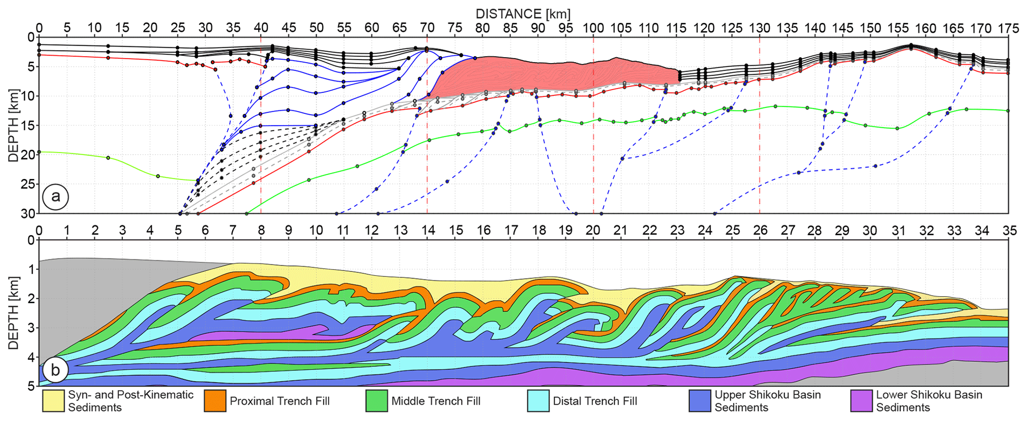
Figure 2(a) 2D structural skeleton – inline section at y=0 km; lines represent interfaces: solid black – shallow sediments; solid blues – inner wedge; solid red – top of the crust; solid green – Moho; dashed black – underplated sediments; grey – subducting sediments; dashed blue – major faults; shaded red denotes outer wedge. (b) Structure of the accretionary prism adopted form (Kington, 2012).
To create an overall skeleton of the model, we start from the interfaces that shape the mantle and the crust. In Fig. 2a, the top of the oceanic or continental crust and mantle are marked by solid red and green lines respectively. The geometry of the subducting slab is inferred from previous studies in the Tokai area. The oceanic crust exhibits variability of thickness and local bending consistently with what is proposed by geological studies in the same region (Kodaira et al., 2003; Le Pichon et al., 1996; Lallemand et al., 1992; Górszczyk et al., 2019) and addressed as an effect of subducting volcanic ridges and sea mounts. On the right flank of the model (starting at 140 km of model distance), we introduce a large volcanic ridge indicated by the uplift of the bathymetry and the significant thickening of the oceanic crust. A similar ridge (Zenisu Ridge) really exists in the eastern part of the Nankai Trough. It currently approaches the subduction zone and simultaneously undergoes the thrusting process (Lallemant et al., 1989).
In the next step, we cut the subducting oceanic crust and mantle by series of interfaces (blue dashed lines in Fig. 2a) to subdivide them into several polygons. These interfaces allow us to project each of the defined block independently in the third dimension (see next Sect. 2.2). They are also designed to implement tectonic discontinuities in the oceanic crust and upper mantle. Such discontinuities acting as faults and thrusts or creating horst-graben structures are well documented in subduction zones (Tsuji et al., 2013; Ranero et al., 2005; Azuma et al., 2017; Boston et al., 2014; Vannucchi et al., 2012; von Huene et al., 2004). At the edge of the continental part, two blue dashed lines mark major boundaries creating large flower-like structures, which can be typically found around strike slip faults zones (Huang and Liu, 2017; Ben-Zion and Sammis, 2003; Tsuji et al., 2014). Each of those boundaries can also be further used to implement fluid paths or damage zones.
On top of the oceanic crust, we place two layers of subducting sediments (grey dashed and solid lines in Fig. 2a). They extend starting from the subducting channel up to the right edge of the model. In general, the lower layer is thicker and overlays directly the top of the oceanic crust covering its thrusts and faults. The upper layer is thinner, whereas its upper limit delineates the decollement in our model. To provide more complexity, we introduce a small duplexing structure within those two layers (between 65 and 85 km in Fig. 2a) similarly to the decollement model presented by Kameda et al. (2017), Hashimoto and Kimura (1999), and Collot et al. (2011).
Just between the edge of the continental crust and the subducting slab, we add a stack of relatively thin sheets corresponding to progressively underplated material (dashed black lines in Fig. 2a). Typically these kinds of structures occur when sediments, which move down on top of the subducting oceanic crust, create a duplex system and are further added to the accretionary wedge (Angiboust et al., 2014, 2016; Menant et al., 2018; Agard et al., 2018; Ducea and Chapman, 2018). Including these relatively fine-scale structures in the deep part of the model will significantly affect wavefield propagation.
The accretionary wedge consists of two parts. The landward part is formed by large deformed stacked thrusts sheets (solid blue lines in Fig. 2a) corresponding to the old accretionary prism, which extends seawards into large out-of-sequence thrusts acting as a backstop now. Similar inner-wedge structures can be found in various subduction zones (Dessa et al., 2004; Raimbourg et al., 2014; Shiraishi et al., 2019; Collot et al., 2008; Cawood et al., 2009; Contreras-Reyes et al., 2010) and can also be modelled with analogue sand-box experiments (Gutscher et al., 1998, 1996). The outer-wedge (red shaded polygon in Fig. 2a) contains the sedimentary prism adapted from Kington and Tobin (2011) and Kington (2012) (Fig. 2b). It is built from different types of sediments, which underwent deformation and created a sequence of thrusts interpreted within the Kumano Basin. The complexly shaped, small-scale, steeply dipping structures will impose a challenge for seismic imaging. In our implementation the prism from Fig. 2b is managed as a single block associated with the respective red shaded polygon in Fig. 2a. Depending on the changes in the shape of this polygon during the projection step, we re-sample the prism from Fig. 2b such that it conforms to the shape of the polygon.
Finally, the frontal prism is fed by the layers of incoming sediments (black lines in Fig. 2a) – relatively thick in the area of the trench and thin over the volcanic ridge. These sedimentary layers are associated with those interpreted in Fig. 2b. Similarly, on the landward part of the model, we implement a sedimentary cover on the backstop including the fore-arc basin over the old part of the prism (between 40 and 70 km). The whole model is covered with a water layer with strongly variable bathymetry.
2.2 Projection
The next step in our scheme is the geologically guided projection of the initial skeleton (Fig. 2a) into the third dimension. We design the set of projection functions that translate the initial inline skeleton in the crossline direction, such that the resulting structure follows concepts related to geology variations along the strike direction. For each new inline section, the initial (xn(y0), zn(y0)) coordinates of the node n (dot in Fig. 2a) are firstly projected in the crossline direction with an arbitrarily chosen deterministic function of the crossline distance y. In this way for a given inline i we obtain a new node n with the coordinates (xn(yi), zn(yi)). The general formula of the projection functions can be expressed as a parametric equation of the following form:
It can immediately be seen that x(y) and z(y) are quadric and linear functions respectively, which control curvature and dipping of a projected structure with the crossline distance yi where . The coefficients an, bn, cn, dn, and en are set up and tuned separately for each node n in Fig. 2a, such that after the projection, they follow the shape of pre-designed geological structures and at the same time maintain their conformity.
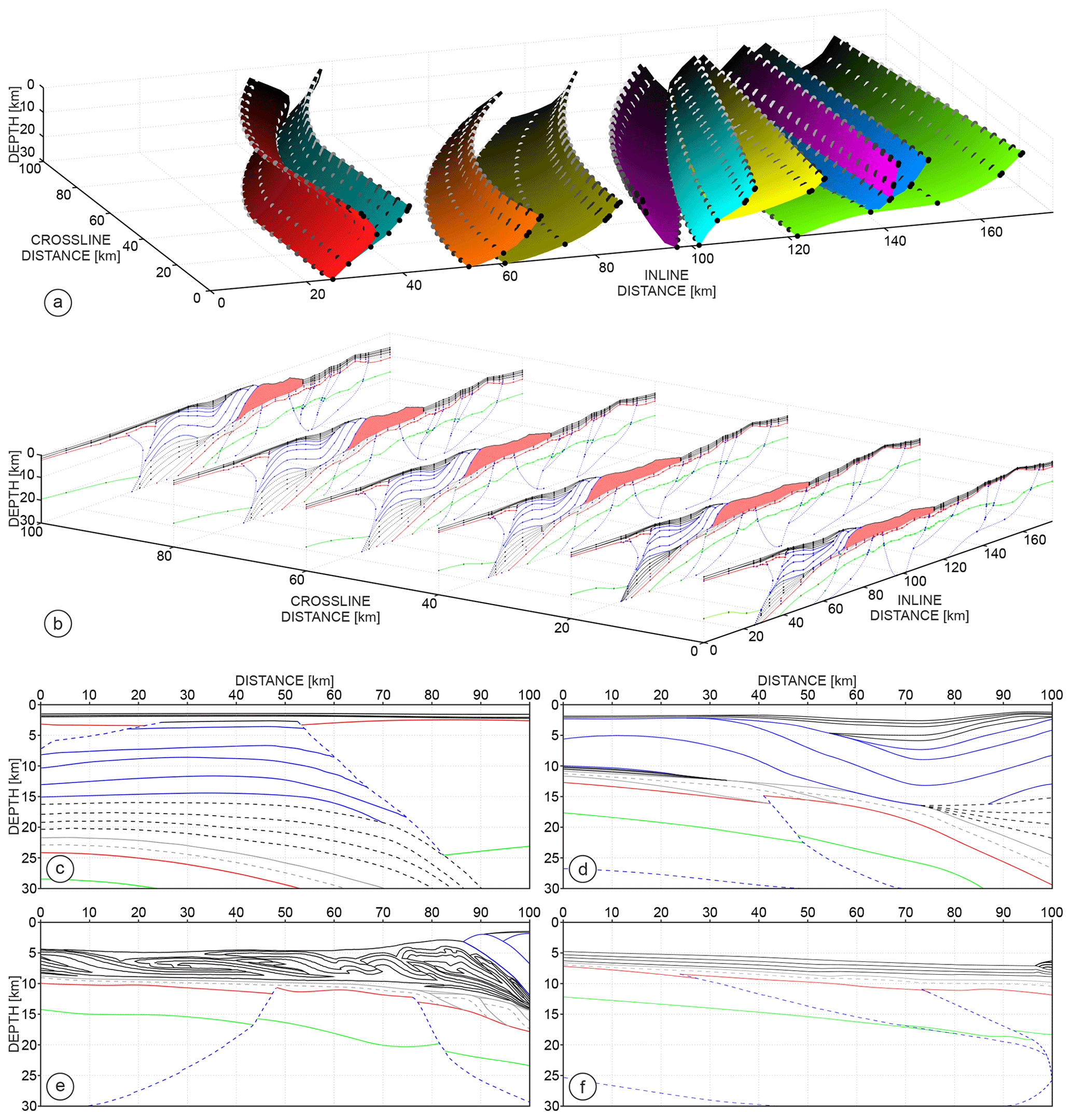
Once the nodes defining a given interface are projected in the crossline direction, we interpolate the piecewise cubic polynomials between the new nodes in the inline direction. In this way we create a new interface, which is slightly shifted with respect to that of the previous inline section. The functions used to project each of the node from the subset of nodes defining a given interface are designed such that they are similar but not exactly the same. This means that the interface is not only shifted (as if exactly the same projection function was used for all the nodes defining the interface) but its geometry can also be modified. In Fig. 3a we show the main fault planes of the model obtained during the projection of the nodes (dots extracted at each 5 km of crossline distance) defining the corresponding interfaces. The figure highlights how the dipping and bending of the presented surfaces, as well as their spatial extension in the (x,z) planes, vary in the crossline direction. From this, it is clear, that based on geometrical constraints (which may describe the complex geological evolution), we are able to modify the shape of the polygons as we project the interfaces from one inline section to the next. The position of the nodes of a given interface can also be defined according to the position of the nodes of another interface. For example, the nodes discretizing the interface marking the top of the subducting sediments (Fig. 2a, grey dashed and solid lines) can be easily defined (shifted up) once we know the coordinates of the nodes defining the top of the oceanic crust (Fig. 2a, red line).
It is worth mentioning that some nodes can belong to several interfaces – for example, when they are at the junction of two interfaces. In such a case, these nodes are projected only once with the function assigned to the first interface in order to guarantee a conform space warp of the polygons. Therefore, the projection function applied to the second interface must be partially determined by the fact that one of the nodes (which belongs also to the first interface) was already projected. In such a way, the structural skeleton we create can be viewed as a system of interfaces that are implicitly coupled via the dependencies between the position of the nodes which define them. Therefore, adding new features to the model or modifying existing ones requires careful design of the corresponding projection functions, which will honour the previous dependencies between interfaces.
We assumed that the model will be 100 km in width, therefore we generate 4001 2D inline sections spaced 25 m apart. To highlight the lateral variability of the structure generated during the projection, we show the skeleton of the inline sections in a perspective view extracted every 20 km (Fig. 3b). First, we design the curved shape of the subduction front. With increasing crossline distance, the oceanic crust and mantle shrink back. As a result, the continental part of the mantle and crust elongates seaward. Simultaneously, we compress and extend the respective polygons making their relative size variable. One can track this variability by following the geometry of the interfaces cutting through the oceanic mantle and crust along successive inline sections (blue dashed lines in Fig. 3b). The absolute depth of the oceanic crust not only changes along the subduction trend but also gently increasing with crossline distance. Simultaneously, there is an up-growing of the underplating sediments below the edge of the continental crust (black dashed lines in Fig. 3b) – consistent with the thickening of the subducting sediments as the crossline distance increases. The position of the backstop also changes from one inline to another. This partially results from the curved shape of the subduction front and was inspired by the 3D interpretation of Tsuji et al. (2017). At the same time, the length of the inner wedge (solid blue lines) increases. This is coupled with the differences in scale and deformation of the thrusts sheets that are building this unit, as well as with the shape of the forearc basin covering it. Further seaward, the outer wedge (i.e. accretionary prism – red shaded polygon) becomes shorter and thicker as the crossline distance is increasing. The right flank of the model is marked by the uplift of the bathymetry related to the presence of the incoming volcanic ridge which becomes smaller as the crossline distance increases.
In Fig. 3c–f, the crossline sections extracted at 40, 70, 100, and 130 km (vertical red dashed lines in Fig. 2a) highlight the structural heterogeneity in the crossline direction. This heterogeneity is defined at different scales. Firstly, due to the overall curved shape of the subducting front. Secondly, due to the different projection functions causing warping of the polygons. The structural complexity will be further increased through parameterization and the application of stochastic components.
2.3 Parameterization
2.3.1 Index and gradient matrix
Once the inline section has been projected in the crossline direction, the newly generated structural skeletons are further mapped into uniform 2D Cartesian grids of the dimension 1201×7001 (grid size 25 m×25 m). During this step, we assign an arbitrary index to the grid points representing different geological units. That is, the grid points inside each of the polygons are now described by a unique integer value. By re-sampling, in the horizontal and vertical directions, the matrix containing the digitized accretionary block shown in Fig. 2b, we reshape its geometry such that it fits to that of the corresponding polygon (red shaded area in Fig. 2a) in each projected inline section. The deformed sediment layers inside the outer wedge have indexes consistent with those of the sediment layers coming into the trench since they represent the same geological formations. Filling all the polygons with the corresponding indexes leads to the matrix plotted in Fig. 4a. We pick random colours to distinguish between the neighbouring units. The matrix contains 46 geological blocks defined by the unique integer index. Such indexation allows us to easily refer to a particular structural unit of the model during the further steps – for example to modify the parameterization.

Figure 4(a) Index matrix with the 46 geological units marked by randomly picked colours. (b) Gradient matrix used for implementation of spatial variations within those units. (c) 2D inline obtained after assigning Vp values to the matrices shown in (a, b).
On top of the index matrix, we implement another matrix, referred to as gradient matrix, which allows us to introduce spatial variations in the physical parameters in each large-scale unit and around the main fault planes (Fig. 4b). Without this second matrix, the physical parameters in each geological unit would have constant value (related to the integer from matrix of indexes). The spatial variation in the parameters within the same unit can be related to increasing depth in the mantle, layering of the crust, low-velocity zones in the subducting sediments, compaction in the prism or damage zones around the faults, etc. We implement those variations using horizontal and/or vertical gradient functions (i.e. linear interpolation functions). These functions can be easily modified and hence provide the necessary flexibility to update the variations in the physical parameters in the structural units. The gradients in Fig. 4b contain float values, which are normalized between 0 and 1 for each unit. The exceptions are the three units in the oceanic mantle (which do not reach the bottom of the model), as well as shallow sedimentary layers and water column (no gradient implementation).
In practice, the index matrix and the gradient matrix are combined to implement any physical parameter in each geological formation. To do so, we extract a given geological unit (based on the index matrix) and assign to it a constant parameter value pα. We also extract the corresponding part of the gradient matrix and denote it by Gn (normalized gradient matrix). The gradient function associated with Gn can be manipulated (scaled, clipped, biased, etc.) leading to the matrix G which provides a desired spatial variation in a parameter in a geological unit. The overall formula to compute the physical parameters inside a given model unit is as follows:
where p(x,z) is the parameter entry at the position (x,z), while pβ scales the entry g(x,z) of G with appropriate physical units.
To better illustrate how the index and gradient matrix can be used to produce a physical model, we consider the following example. Let us imagine that we want to assign Vp values inside the part of the oceanic crust delineated by the thick red line in Fig. 4a and b. The integer index assigned to this unit is 11 (Fig. 4a). We set pα to 4800 m s−1 and pβ to 2300 m s−1. Taking into account that the values of Gn for this unit span 0.0 to 1.0 (from the top to the bottom of the crust), the final Vp values will be increasing linearly from 4800 to 7100 m s−1. One may also desire to implement a gradient discontinuity in the oceanic crust corresponding to the oceanic layer 2–layer 3 boundary. Setting the thickness ratio to 0.3 and 0.7 in layer 2 and layer 3 respectively would split Gn in unit 11 into two sub-matrices given by
As a result, we obtain two gradient matrices G1 and G2 with normalized values between 0.0 and 1.0. We can now set the pα to 4800 m s−1 and pβ to 1600 m s−1 for G1. As a result, we obtain rapid increase in Vp between 4800 to 6400 m s−1 inside layer 2. For G2, we use pα equal to 6500 m s−1 and pβ equal to 600 m s−1 leading to Vp values inside layer 3 ranging between 6500 and 7100 m s−1. The resulting boundary between layer 2 and layer 3 is marked with dashed line in Fig. 4c.
We also use the gradient matrix to implement variations in the parameters within the subducting sediments, fault-related damage zones, and subducting channel, which result from small-scale geological processes (fluid migrations, lithological variations, tectonic compaction, mass wasting, etc.; Agudelo et al., 2009; Park et al., 2010). Moreover, we implement lateral parameter discontinuities at the interfaces acting as faults. For example, the stairs in the Moho resulting from the interfaces cutting through the oceanic mantle and crust imply that the gradients on both sides of those interfaces are slightly different. In consequence, we create a lateral jump in the parameter values on both sides of the fault, which will generate impedance contrast amenable to its imaging. In practice, this jump is more pronounced near the top of the mantle (∼5 to ∼7 km below Moho) and vanishes with increasing depth to completely disappear at the bottom of the model.
Finally, the gradient matrix also describes two additional types of perturbations. The first type is implemented around the regions of thickened oceanic crust mimicking subducting volcanic ridges (Park et al., 2004; Kodaira, 2000). They are marked by the gradient and velocity variations in Fig. 4b and c (95–105 and 145–155 km). The second type of perturbations is intended to introduce more heterogeneity around the fault planes such as damage zones or fluid paths. Parameter variations within such zones affect the kinematic and dynamic characteristic of the propagating wavefield. They also have the potential to generate distinct arrivals – so-called trapped waves (Li and Malin, 2008; Ben-Zion and Sammis, 2003). We implement such anomalies around the faults in the oceanic crust and upper mantle, the major faults at the edge of continental crust, and within the large thrusts sheets between inner and outer accretionary wedge. A few small perturbations are also locally added between layers of the inner wedge to increase the complexity of this unit.
2.3.2 Physical parameters
From the index and gradient matrices described in the previous section, we can now implement the seismic properties in the structural units. In practice, this requires some constraints on the parameters, which might come from field experiments and laboratory measurements. Regional seismic studies often lack resolution to directly map the reconstructed properties into the fine-scale structures of our model. Moreover, they often ignore second-order parameters such as density (ρ), attenuation (Qp and Qs), and anisotropy to focus on the P-wave velocity (Vp) reconstruction, which plays the leading role in the active seismic imaging and can be estimated from the seismic data more precisely than for example density or attenuation. Therefore, we first develop a Vp model from recent FWI case studies in the Nankai Trough. Then, we use this Vp model as a reference to build the other parameters – namely Vs, ρ, Qp, Qs – from empirical relations. Reconstruction of Vp from wide-angle seismic data has long historical records (Christensen and Mooney, 1995; Mooney et al., 1998). Travel time tomography has produced a vast catalogue of smooth Vp models from different regions around the world. This information (even though Vp values can significantly vary depending on the studied area) is useful to constrain the velocity trend in the main large-scale geological units (such as mantle, continental, and oceanic crust). Moreover, recent OBS FWI case studies partially fill this resolution gap (Kamei et al., 2012; Górszczyk et al., 2017) and allow us to refine Vp in the short-scale units of our model (Fig. 4c). We perform this refining of the Vp velocities by trial and error, until the OBS gathers simulated under acoustic approximation in the Vp model exhibit overall a similar anatomy to the OBS gathers collected during 2001 Seize France Japan (SFJ) OBS survey in the eastern Nankai Trough. In Fig. 5a and b, we present a qualitative comparison of the field and synthetic gathers for the OBS stations located above the backstop of the Tokai segment and the backstop of the velocity model presented in Fig. 4c (30 km of model distance). Despite the different offset ranges and recording times (we extend it for the synthetic data to compensate for the deeper water than in the field data), the synthetic gather exhibits the same types of arrivals appearing in relatively similar order as in the case of the field data. This similarity justifies a sufficient level of kinematic realism of the Vp values for the purpose of our geomodel.
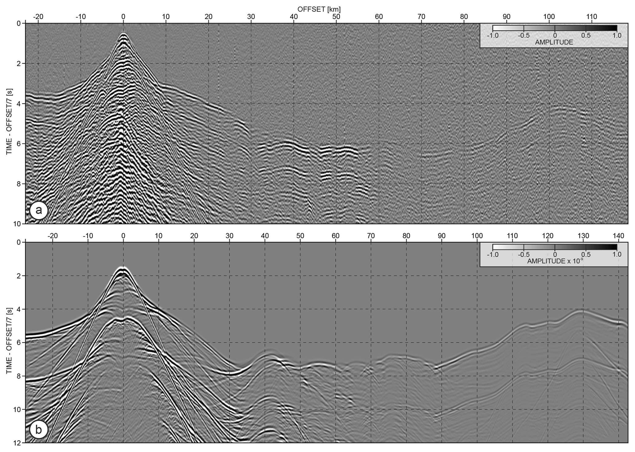
Figure 5Comparison of the (a) field and (b) synthetic OBS gathers. The gather in (a) comes from the OBS 21 of the SFJ OBS 2001 experiment, while the gather in (b) comes from the waveform modelling for the OBS located at 30 km model distance of the 2D inline model presented in Fig. 4c.
From the Vp model, we build Vs and ρ using the empirical polynomial relations of Brocher (2005). These relations were inferred from compiled data on laboratory measurements, logs, vertical seismic profiling, and tomographic studies. They are relevant for Vp ranging from 1500 to 8500 m s−1 and hence represent the average behaviour of crustal rocks over the depth range covered by our model. The resulting Vs and ρ models are presented in Fig. 6a and b. Shear-wave velocities in the shallow sediments are as small as ∼530 m s−1. Although even lower velocities can be found in the first few metres below the seabed, these values already impose significant challenges for wavefield modelling. In the oceanic crust, Vs increases from 2900 to 4000 m s−1, while it starts at 4500 m s−1 on top of the upper mantle and gently increases with depth. Density of the oceanic and continental crust varies from 2500 to 3000 kg m−3 and from 2500 to 2900 kg m−3 respectively, while in the upper mantle ρ starts around 3200 kg m−3. Figure 6c shows the ratio, which varies from 1.6 to 3.0. Initially, the Vs model obtained from empirical relations of Brocher (2005) was not producing a heterogeneous ratio in the subduction channel – as it can occur when fluid overpressure, fluid diffusion, or hydro-geologically isolated zones generate variation in the seismic properties in the subduction channel (Kodaira et al., 2002; Collot et al., 2008; Ribodetti et al., 2011). Therefore, we additionally rescale the velocities in this unit using the index and gradient matrices.
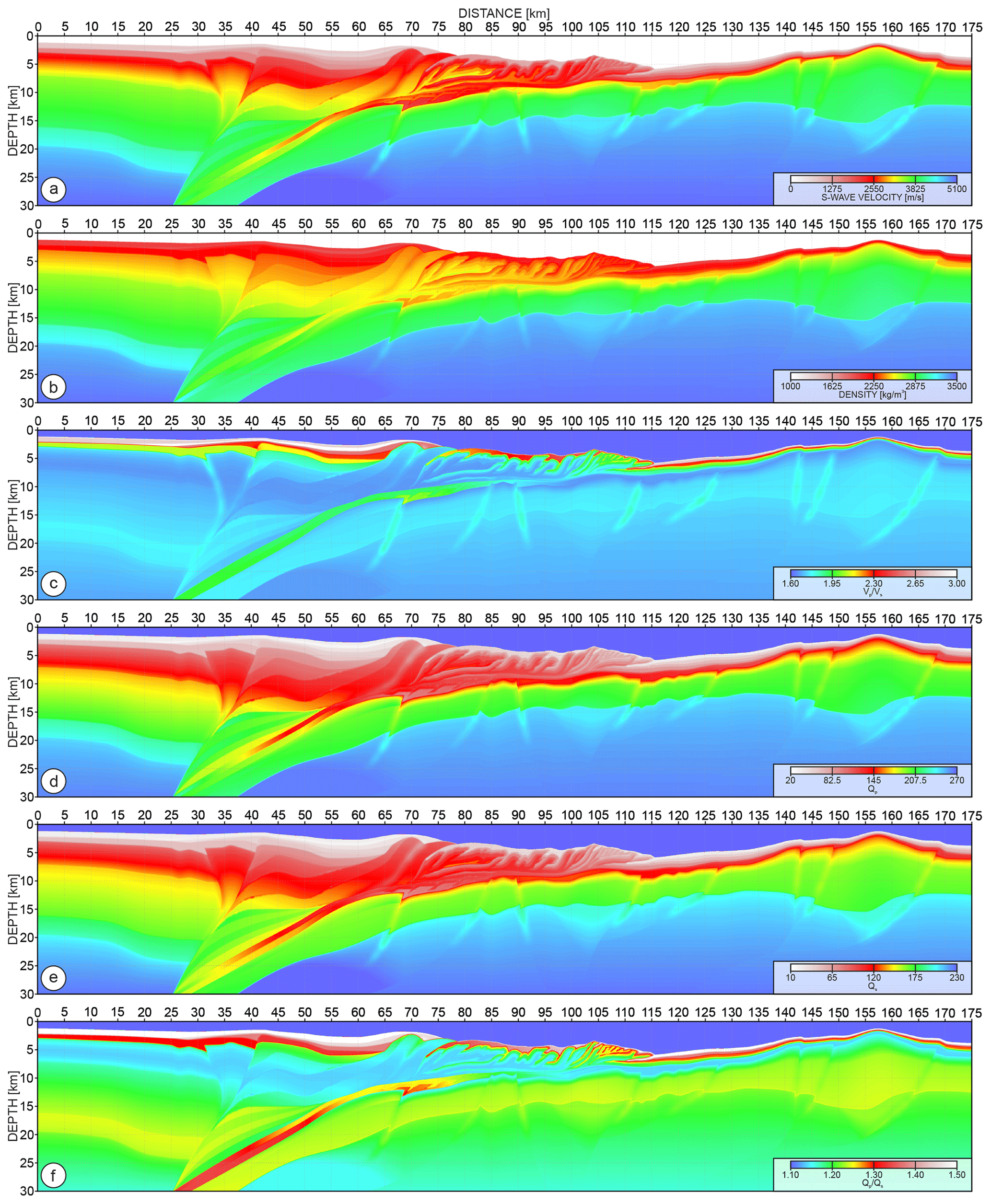
Figure 6(a) Vs, (b) ρ, (c) , (d) Qp, (e) Qs, (f) models derived from the Vp inline from Fig. 4c.
We also implement attenuation effects in our model through the Qp and Qs parameters. The choice of consistent approach to constrain plausible Qp and Qs models is quite challenging. This is firstly because the various types of attenuation (intrinsic and scattering-related) can be controlled by countless factors – rock type and mineralogy, porosity, fluid content and saturation, temperature, etc. Secondly, values of the Q factor can differ significantly between studies depending on the methodology used, the scale of the attenuation, or the frequency content of seismic data. Thirdly, accurate reconstruction of Q models from field experiments is not as well documented because the footprint of attenuation in the wavefield remains small in particular in the deep crust. Therefore, to build the Qp and Qs models, we combine few empirical relations between velocity (Vp, Vs, ) and attenuation (Qp, Qs), which we find consistent for our synthetic model. To build the Qs model, we use the following power law (Wiggens et al., 1978). This empirical relation is in good agreement with the Qs estimation of Olsen et al. (2003) performed in the Los Angeles Basin. The estimated Qs values range from ∼25 in the shallowest sediments to ∼220 in the deep mantle (see Fig. 6e). To avoid a constant ratio between Qp and Qs (Qp=1.5Qs in Olsen et al., 2003), we generated the Qp model (Fig. 6d) via another empirical relation – derived from well-log data by Zhang and Stewart (2008). This formula, even though derived from velocities up to ∼3000 m s−1 using a sonic-log frequency band, produces reasonable Qp variations between ∼35 and ∼260 in our model and leads to a ratio ranging from ∼1.1 to ∼1.5 (Fig. 6f), which is in good agreement with the values estimated in the Mariana subduction zone (Pozgay et al., 2009). The small Q values in the shallow sediment layers and/or subducting channel will significantly affect the short to intermediate offset wavefield. On the other hand, the higher Q values in the crust and mantle can still affect the ultra-long-offset waves penetrating for a long time through these parts of the model. The Q values we define here are related to the intrinsic attenuation during the wavefield propagation. Additionally, the attenuation of high-frequency wavefield component through the scattering effects is introduced in our model by the means of small-scale stochastic perturbations as described in the following section.
2.4 Stochastic components
In the final step of our model-building procedure, we consider various types of stochastic components, which are intended to introduce perturbations of a random character into the model. We design two types of such random components: (i) small-scale parameter perturbations and (ii) spatial warping of the final 3D cube.
2.4.1 Small-scale perturbations
In Figs. 4c and 6, the parameters vary smoothly within the units according to the applied gradient functions. Indeed, such smooth variations are a rather idealized vision of the true earth. Therefore, to make it more realistic, we create another matrix describing small-scale perturbations (Fig. 7a), which will have a second-order impact on the wavefield propagation. Using this matrix, we can scale the models after parameterization and obtain the updated model presented in Fig. 7b (compare with the smooth velocity variations in the Vp model shown in Fig. 4c). The inset in Fig. 7b shows the symmetric histogram (with a distribution close to normal) of the introduced velocity changes ranging between −300 to 300 m s−1. The matrix in Fig. 7a is obtained by stacking 3D disk-shaped structural elements (SEs) (Fig. 7c–f). The values in the SEs (Fig. 7g) vary from 0 at the edge to 1 at the centre and are further translated into parameter perturbations. We can control the position and size of these SEs, as well as their correlation lengths (z, x, y) – depending on a desired characteristic of the final perturbations.
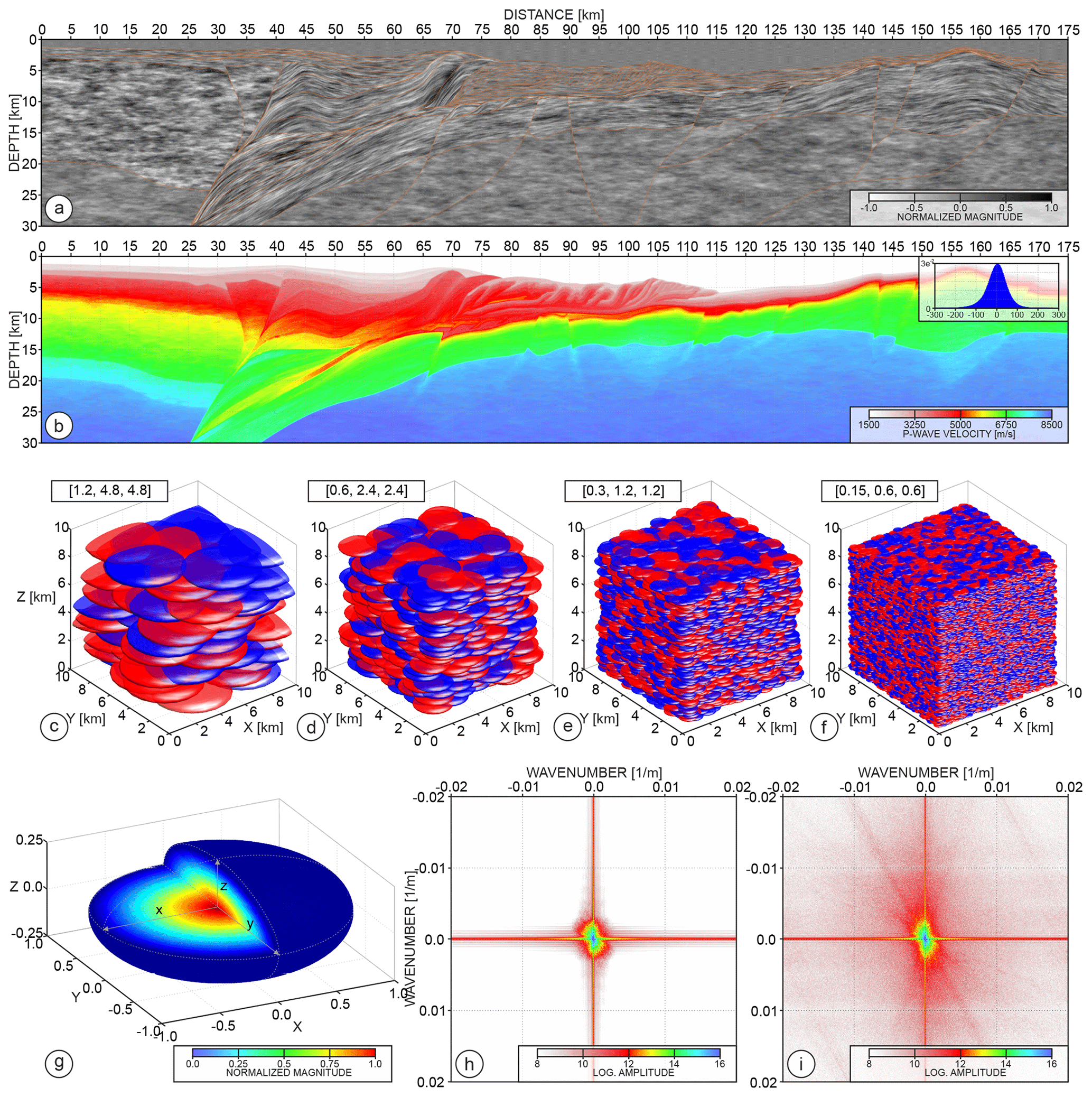
Figure 7(a) Matrix of stochastic perturbations for a 2D inline section. (b) Vp model shown in Fig. 4c after the application of the stochastic perturbations shown in (a). (c–f) 3D stack of structural elements of different scales – see the correlation lengths in brackets. Red/blue colours indicate positive/negative magnitudes of the stacked structural elements. (g) Shape of the 3D structural element used to generate the stochastic perturbations. (h, i) Wavenumber spectrum of the 2D Vp inline section with and without stochastic perturbations.
In Fig. 7c–f, we show four different 3D stacks ( sub-volumes are displayed), corresponding to four different scales of the SEs with a correlation length ratio equal to . The red/blue colours correspond to the positive/negative amplitudes, which are randomly assigned to each of the SEs during stacking. These random variations in positive/negative amplitudes guarantee that the final distribution of the stochastic perturbations for each geological unit in the matrix shown in Fig. 7a has a zero mean. The position of the SE within the stack is controlled by the Cartesian coordinates. The distances between the centres of neighbouring SE equal (, , ), where rz, rx, and ry are the spatial shifts randomly picked from the intervals (, ), (, ), and (, ). In other words, the neighbouring SEs strongly overlap each other – as can be seen in Fig. 7c.
Looking at the stochastic matrix in Fig. 7a, one can observe that the scale, shape, and direction of the perturbations vary from one geological unit to another. For example, perturbations in the prism are finer than those in the crust or mantle. Also, their shape in the oceanic crust and prism are more anisotropic than the shape of those implemented in the mantle. In practice, this is implemented by summation of 3D stacks containing different SEs. For example, we create stochastic perturbations in the sedimentary layer and the outer prism with only the SEs shown in Fig. 7e and f. Perturbations in the inner wedge and underplated units additionally incorporate SEs shown in Fig. 7d. Finally, the oceanic crust contains SEs at all scales (Fig. 7c–f). This also applies to the mantle and continental crust; however, for these units we use an SE with different correlation length ratios equal to . Due to the strong overlapping of the SEs and the superposition of SEs of different scales, the range of the magnitude inside the final 3D stacks significantly exceeds ±1. Therefore, after staking procedure, we re-normalize the 3D stochastic perturbation matrices between −1 and 1.
In Fig. 7a, we also show that the stochastic perturbations in some of the units are oriented according to the dipping or bending of the structure. Since we know the polynomials defining each of the interfaces in the model (and therefore their position), we shift vertically the columns of the matrix containing stochastic perturbations of a given geological unit such that they follow the shape of the structure. For example, the perturbations that fill the oceanic crust follow the smooth trend generated from the polynomial approximation of the interfaces creating the top of the oceanic crust. Note, that because we stack truly 3D SE, within the 3D cube of the same size as the 3D model, our stochastic perturbations continuously follow the geological structures not only in the inline direction but also in the crossline direction.
To analyse what the designed stochastic perturbations mean in terms of the spatial resolution of the model, we compute the 2D wavenumber spectrum (displayed in logarithmic amplitude scale in Fig. 7h, i) of the Vp model with and without stochastic components. As shown in Fig. 7h, the spectral amplitudes of the model without stochastic perturbations are focused around the low-wavenumber part of the spectrum, which represents structures the size of which is of the order of ∼500 m and larger. In contrast, the high-wavenumber amplitudes are clearly magnified in the spectrum of the model with stochastic components (Fig. 7i). The overall spatial distribution of the energy added to the background medium with respect to the spectrum shown in Fig. 7h is broad, which highlights the randomness of the perturbations. The designed approach led to perturbations of a smaller size in fact being of the order of the grid size (25 m). On the other hand, one can also observe in Fig. 7i a few dipping bands of increased amplitudes. They correspond to the anisotropic shape of the SEs following the geological structures – and therefore indicate that our stochastic perturbations are partially predefined and not purely random.
2.4.2 Structure warping
Finally, we apply a second type of stochastic components to the model after projection, parameterization, and application of small-scale stochastic perturbations. The aim of this step is to perform a small-scale pointwise warping of the input 3D grid using a distribution of random shifts. By small-scale we mean that the structural changes introduced by warping are in general much smaller than those incorporated during the projection step. Their impact on the shape of the wavefield will therefore be weaker than the one induced by the geological structure itself but more pronounced than that resulting from the small-scale perturbations described in the previous section. The idea was inspired by dynamic image warping (DIW) (Hale, 2013). DIW is a technique which allows for the estimation of local shifts between two images (2D matrices), assuming that one of the images is a warped version of the other image. This problem is cast as an inverse problem where the unknowns are the shifts that will allow for matching between the two images.
In our case, we use DIW in a forward sense. This means we build a matrix of smoothly varying random spatial shifts of a desired scale and magnitude. Then, we warp each of the inline section from the 3D model grid using those shifts. Figure 8a and b show two 300 km×300 km matrices that represent distribution of shifts for two different spatial scales. While the scale of the shifts in Fig. 8a is local (starting from ∼10 km), the spatial extension of the shifts in Fig. 8b is regional. The blue and red colours indicate the negative and positive shifts respectively – scaled between ±2 km. To obtain those matrices, we first generate the matrix of the same size with the random values from the interval. In the second step we interpolate between the uniformly subsampled (in both directions) elements of this random matrix using spline functions. The spatial scale of the final shifts is controlled by the subsampling of the matrix with random values – that is, the dense or sparse subsampling leads to small- or large-scale of perturbations. After interpolation, we scale the values in both matrices to obtain the desired magnitude of the shifts (in this case ±2 km). We take the average of the two distributions to obtain the final distribution shown in Fig. 8c. Our procedure of warping is implemented as follow.
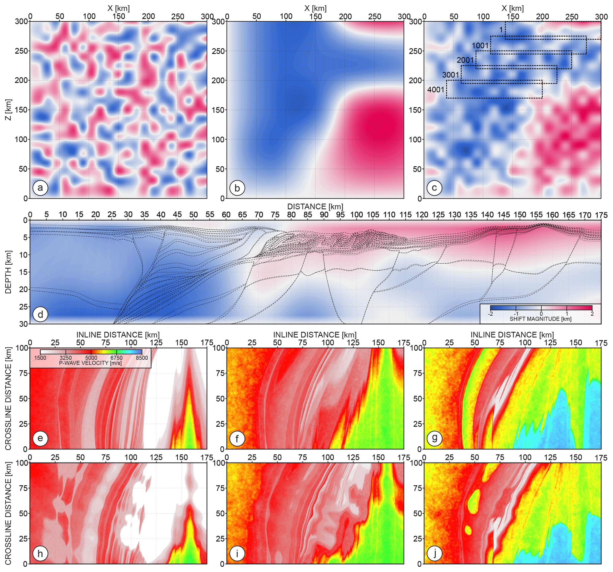
Figure 8(a, b) Spaces of random small- and large-scale spatial shifts respectively; (c) final space of shifts – average from (a, b). Dashed rectangles mark extracted matrices of shifts for inlines at each 20 km of crossline distance; (d) matrix of shifts extracted from (c) (black dashed rectangle number 1). Grey solid and black dashed lines represent the structure before and after warping respectively; (e, f, g, h, i, j) depth-slice sections extracted at 5, 7.5, and 10 km before and after warping respectively.
First, for each of the 4001 inline sections, we extract from the distribution shown in Fig. 8c a 2D sub-matrix with the size of the inline section. Figure 8d shows such a matrix corresponding to the first inline section – marked by to the black-dashed rectangle in the upper-right corner of Fig. 8c. The further rectangles in Fig. 8c illustrate how we move from one sub-matrix to another one for five inline sections spaced 20 km apart (inline number 1, 1001, 2001, 3001, and 4001).
Once we have the sub-matrix of shifts and the initial inline section mi(x,z), the warped inline section mw(x,z) is obtained by the identity , where s is the entry of the sub-matrix of shifts at the (x,z) position. In Fig. 8d, the warped structure (dashed black lines) is shifted downward and upward with respect to the initial structure (solid grey line) for negative (blue colour) and positive (red colour) shifts respectively. For simplicity, we consider only vertical shifts in this example. However, we also implement warping in the horizontal direction, i.e. , in the same way as we do in the vertical direction.
Once an inline section has been warped, we extract a sub-matrix of shifts for the next inline section from the distribution of shifts shown in Fig. 8c. We perform this extraction at a slightly modified position with respect to the previous one, typically one grid point further (i.e. 25 m). In this way, we maintain the continuity of the warped structures along the crossline direction. Although this inline-by-inline procedure is based on the 2D warping, in practice it introduces fully 3D structural changes in the model, at the same time remaining more practical for quality control of the results and computational efficiency.
Three depth slices extracted at 5, 7.5, and 10 km depth from the 3D Vp models before and after warping highlight how the warping has modified the shape of the structures (Fig. 8e–g). Importantly, the continuity of the structure is preserved during warping not only along the inline direction but also along the crossline direction. It is also worth remembering that, in this example, the distribution of shifts is random. However, nothing prevents using a deterministic distribution, for example to produce uplift or bending of certain parts of the model.
In this section, we perform full wavefield modelling in a target of the GO_3D_OBS model to assess the footprint of the structural complexity and the heterogeneity of the physical parameters on the anatomy of these wavefields. Figure 9 shows the perspective view of the full 3D Vp model with a chair-plot representation. To perform our modelling experiments, we select a target in the central part of the full model (for each parameter) (white lines in Fig. 9). We simulated OBS gathers, for the station located 10 km apart from the nearest edges of the target (see the white point in Fig. 9) and the air-gun shots at 10 m depth below the sea level. The shooting line is oriented in the inline direction (red lines in Fig. 9) at the position of the inline number 2601. In the next sections, the 2D simulations are performed in this inline model. The source signature is a 1.5 Hz Ricker wavelet (spectrum energy up to 4.5 Hz) and the propagation time is 30 s. We perform modelling taking advantage of the reciprocity principle – that is, we place the pressure sources at the position of the hydrophone of the OBS and extract the pressure component at the position of the air-gun shot. In the following section, we present few examples of 2D and 3D modelling for different approximations of wavefield propagation. The dynamic and kinematic differences between the seismograms resulting from different modelling scenarios underline the significance of the modelling engine and its possible impact on the waveform inversion results. We run the simulations in the time domain using the TOYXDAC visco-acoustic finite-difference (second-order in time and fourth-order in space) and SEM46 viscoelastic spectral-element FWI codes developed within the framework of the SEISCOPE consortium (https://seiscope2.osug.fr, last access: 16 March 2021).
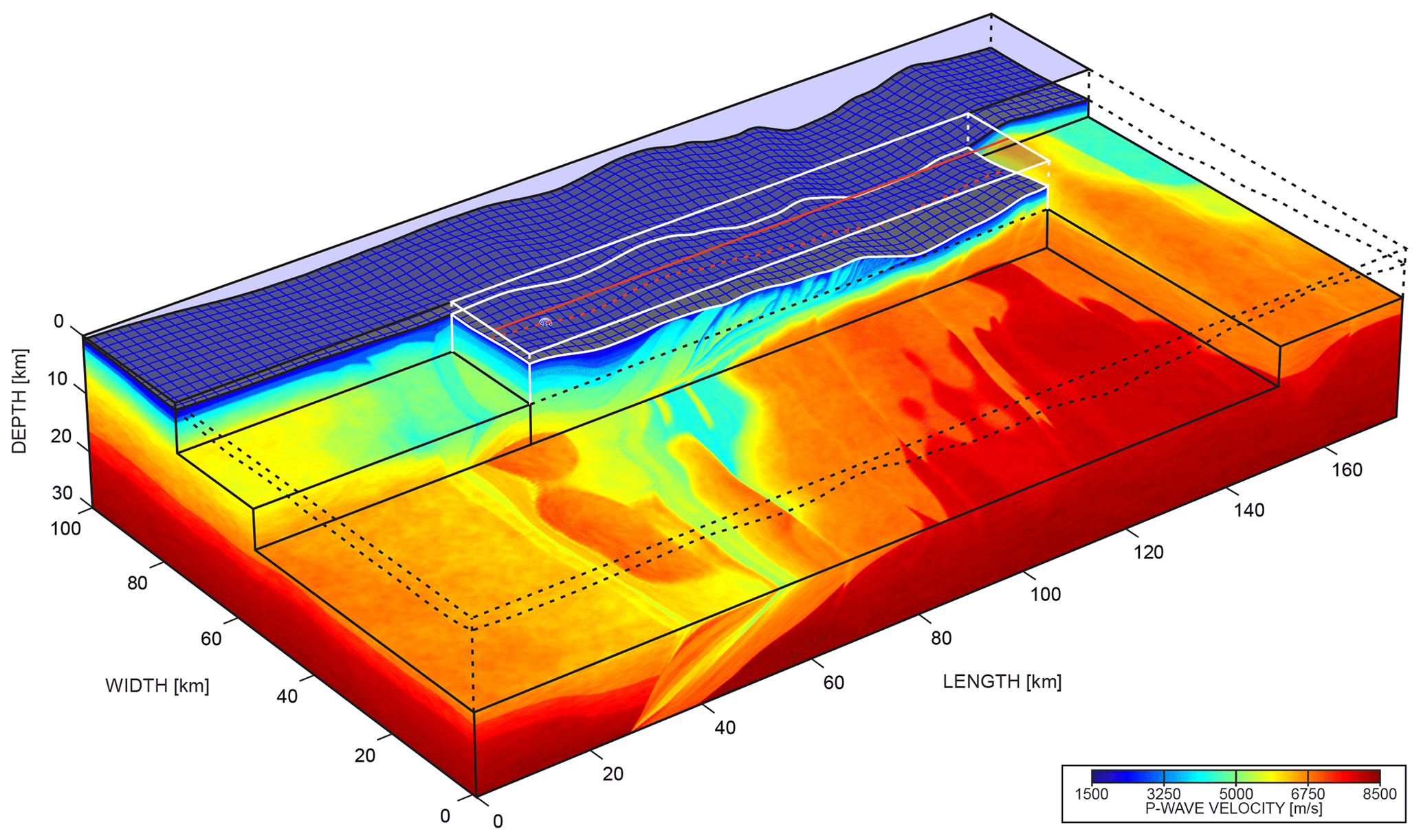
Figure 9The perspective view on the chair plot of the 3D Vp cube. The central volume defined by the white lines corresponds to the part of the model () used for simulation of the data presented in Sect. 3. The white point at the seabed marks the OBS position and the red solid and dashed lines denote the shooting profile and its projection to the bathymetry respectively.
3.1 Acoustic versus visco-acoustic 2D wavefields
The first modelling test demonstrates the influence of the viscous effects on 2D acoustic P-wave modelling. We compare 2D wavefields that are computed without (Qp=10 000) and with attenuation. The intrinsic attenuation mechanism we use is based on the generalized Maxwell body including three standard linear solid attenuation mechanisms (Yang et al., 2016). For the sake of computational costs, all the models are re-sampled in a uniform Cartesian grid with a 50 m grid interval.
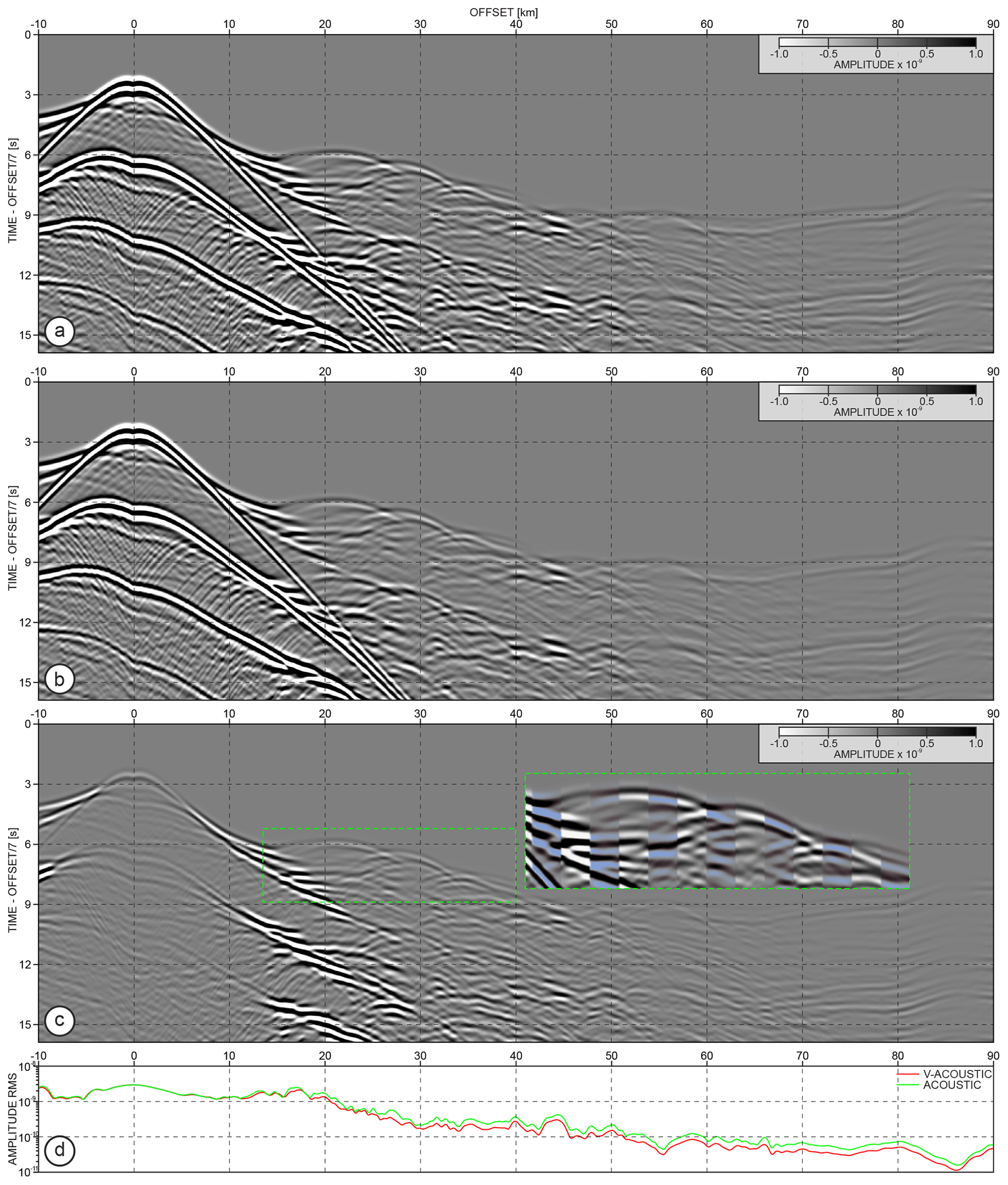
Figure 10OBS gathers generated using 2D finite-difference (a) acoustic and (b) visco-acoustic waveform modelling. (c) Difference between (a) and (b). The inset shows time shifts between the groups of 20 interleaved traces from (a) (blue shading) and (b) extracted within green dashed rectangles. (d) Rms amplitude curves of the gathers from (a, b).
Figure 10a and b shows the OBS gathers generated with constant and variable Qp models. True-amplitude seismograms are plotted in both panels with the same amplitude scale. Although the two gathers look almost identical, the difference between them – shown in Fig. 10c – clearly shows the variations in the signal amplitudes. Changes are mostly visible in the first arrivals up to 15 km offset (corresponding to the waves travelling in the shallow parts of the model), as well as in the energetic reflection from the top of the subducting oceanic crust. This reflection is affected by the high attenuation layer within the subduction channel.
In Fig. 10d, we show in logarithmic scale the root mean square (rms) amplitude variations with an offset for gathers from Fig. 10a and b. The red curve corresponding to the visco-acoustic data is consistently below the green one (indicating the acoustic data). This is a natural consequence of the higher attenuation introduced by the GO_3D_OBS Qp model as compared to constant Qp=10 000 model. Importantly, the variable Qp model introduced not only differences in terms of wavefield amplitude but also notable phase shifts due to dispersion effects. The inset in Fig. 10c shows the zoom on interleaved traces extracted within the dashed rectangles in Fig. 10a and b. Arrivals in the data modelled with variable Qp model (blue-shaded traces) are slightly delayed in time with respect to those simulated with Qp=10 000 (black–white traces). Therefore, incorporating the attenuation model during waveform inversion can not only improve the amplitude reconstruction but it can also have a second-order impact on the kinematic correctness of the final image.
3.2 2D versus 3D visco-acoustic wavefields
We assess now the footprint of 3D effects by comparing the synthetic seismograms computed by 2D and 3D wave modelling. The data resulting from both simulations are shown in Fig. 11a and b. For better readability of far-offset traces, we weight the amplitudes by the absolute value of the offset. Both gathers, of course, have different amplitude versus offset variations due to the different kinds of sources used in 2D and 3D (line sources versus point sources). To bring the amplitudes of the gather resulting from 3D modelling to the same order as in the case of its 2D equivalent, we scale the seismogram in Fig. 11b by the factor of 15 000. The rms amplitude variation with offset curves are presented in Fig. 11c. Apart from this different amplitude behaviour, both gathers look similar at first sight. To better visualize potential 3D kinematic effects, we interleave 20 traces from one gather with the following 20 traces from another one. As a result, we obtain the gather presented in Fig. 11c (the blue-shaded phases correspond to the 2D modelling). Not surprisingly, the mismatch between the two sets of seismograms increases in general with increasing offset and time. For instance, the difference between the first-arrival travel times for the Pn wave reaches ∼150 ms at the far offset (70–90 km offset). However, we also clearly see small time shifts at short and intermediate offsets and more significant time mismatches for the complex package of reflections magnified in the inset in Fig. 11c.
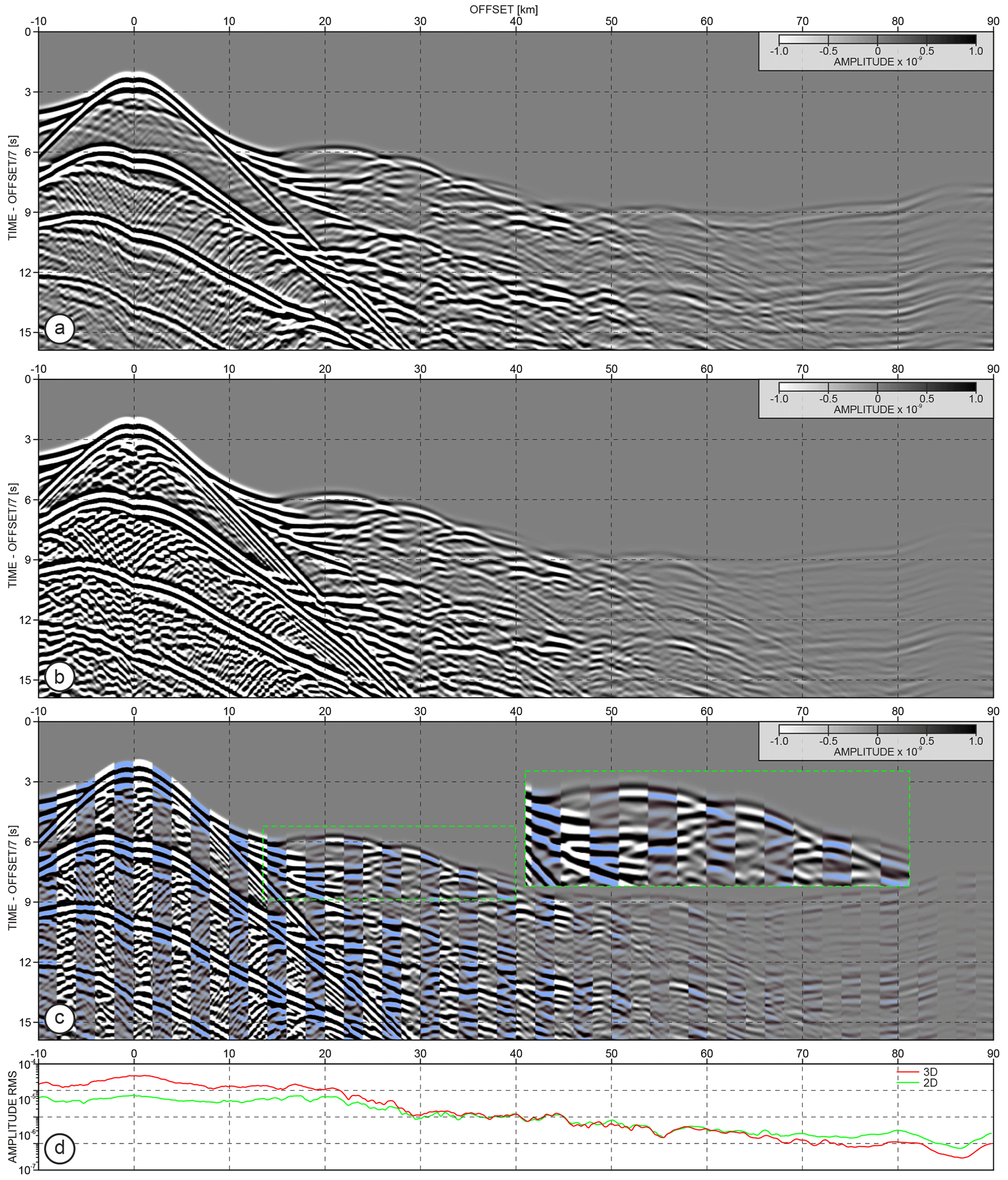
Figure 11OBS gathers generated using finite-difference visco-acoustic (a) 2D and (b) 3D waveform modelling. (c) Comparison of seismograms from (a, b) where 20 traces from 3D modelling are interleaved with the following 20 traces from the 2D equivalent (light-blue shading). For better readability, the seismograms in (a, b) are scaled with the absolute offset value. Seismograms in (b) are scaled by the factor of 15 000 to obtain the same order of amplitudes as in (a). (d) Rms amplitude curves of the gathers from (a, b) – without scaling with offset.
To better understand how the wavefield propagates within the 3D target during the simulation, we extract snapshots every 2.5 s at 10 km depth (see black dotted line in Fig. 9 for the depth-slice location). For comparison, we also perform 3D modelling in the 2.5D version of the inline section number 2601. Depth slices extracted from the Vp 3D and 2.5D models are presented in Fig. 12a. The corresponding snapshots are displayed in Fig. 12b–l. The lower half of each panel (blue-shaded phases) presents the respective snapshot from the wavefield modelling performed within the 2.5D model. It is clear, that with increasing time and offset distance, the wavefield simulated in the 3D target differs more than the 2.5D counterpart. In particular, while the blue-shaded wavefield is symmetric with respect to the shooting profile, the wavefield computed in the 3D target shows evidence of significant off-plane propagation. This is indicated both by the slant appearance of the first arrival wave (Fig. 12d–f), as well as the shape and the spatial location of the reflections. In Fig. 12m, we show an analogous comparison to that in Fig. 11c between 3D and 2.5D seismograms. Although the 2.5D data fit the 3D data better than their 2D counterpart (probably due to the consistent point-source implementation for 2.5D and 3D modelling), the phase shifts between far-offset traces can still be observed. There is also a visible mismatch in terms of later arrivals' phase alignment between the traces in the inset containing a complex reflection package.
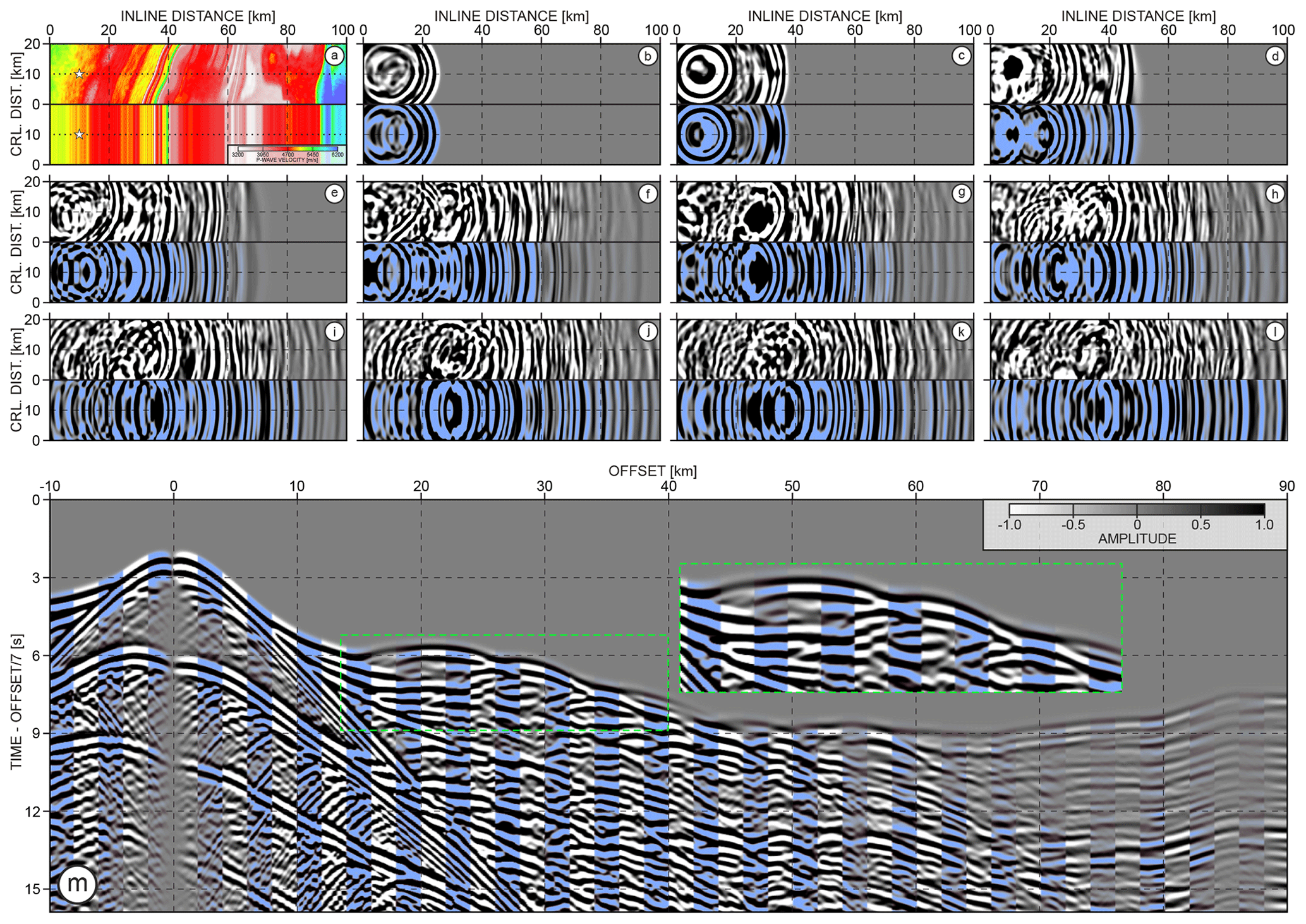
Figure 12(a) Depth-slice sections extracted at 10 km depth from 3D (upper half) and 2.5D (lower half) Vp sub-volumes. White stars and black dotted lines mark the projection of the OBS position and shooting profile respectively; (b–l) snapshots extracted during wavefield modelling at each 2.5 s time step along the corresponding depth slices from (a). (m) Analogous comparison between 2.5D and 3D data as in Fig. 11c. Amplitudes are scaled with the absolute offset value.
Note that, although our 3D target contains part of the curved subduction front, the acquisition profile is still mainly aligned with the dip direction of the structures within the wedge. Nevertheless, the off-plane wavefield propagation is still remarkable. One can imagine that this effect can be further magnified when the geological setting contains more heterogeneities along the crossline direction.
3.3 Acoustic versus elastic 3D wavefields
The final modelling example that we present here shows the difference between 3D spectral-element acoustic (in the whole model) and acoustic–elastic (acoustic in water and elastic in solid) wavefield propagation. The solid–fluid coupling along the bathymetry is implemented by means of displacement potential (Ross et al., 2009). For the acoustic–elastic test, we extract the target from the full Vs model (Fig. 6a). The lowest Vs value in the most shallow sediments covering the backstop area of the model reaches ∼530 m s−1. To speed up the elastic wavefield simulation, we clip Vs to 800 m s−1. This makes it possible to use the smallest element size in the spectral-element mesh equal to ∼213 m (considering the 1.5 Hz Ricker source and fourth-order polynomial interpolation).
Figure 13a and b show the two OBS gathers inferred from acoustic and acoustic–elastic wavefield modelling. One can observe that the package of wide-angle reflections between 20 and 60 km in Fig. 13a contains significantly more energetic arrivals as compared to the same arrivals in Fig. 13b. Some of them are difficult to track (or simply not present) in the gather generated using acoustic–elastic wavefield propagation. This loss of energy can be explained by the P to S conversions. In contrast, we can see in Fig. 13b the weak arrivals of low apparent velocity between 5 and 20 km, indicating some elastic effects. The acoustic and acoustic–elastic seismograms are compared in Fig. 13c in the same way as in Fig. 12c. One can observe that the phases from the acoustics modelling (blue-shaded traces) do not match with their elastic counterpart indicating differences between two types of data.
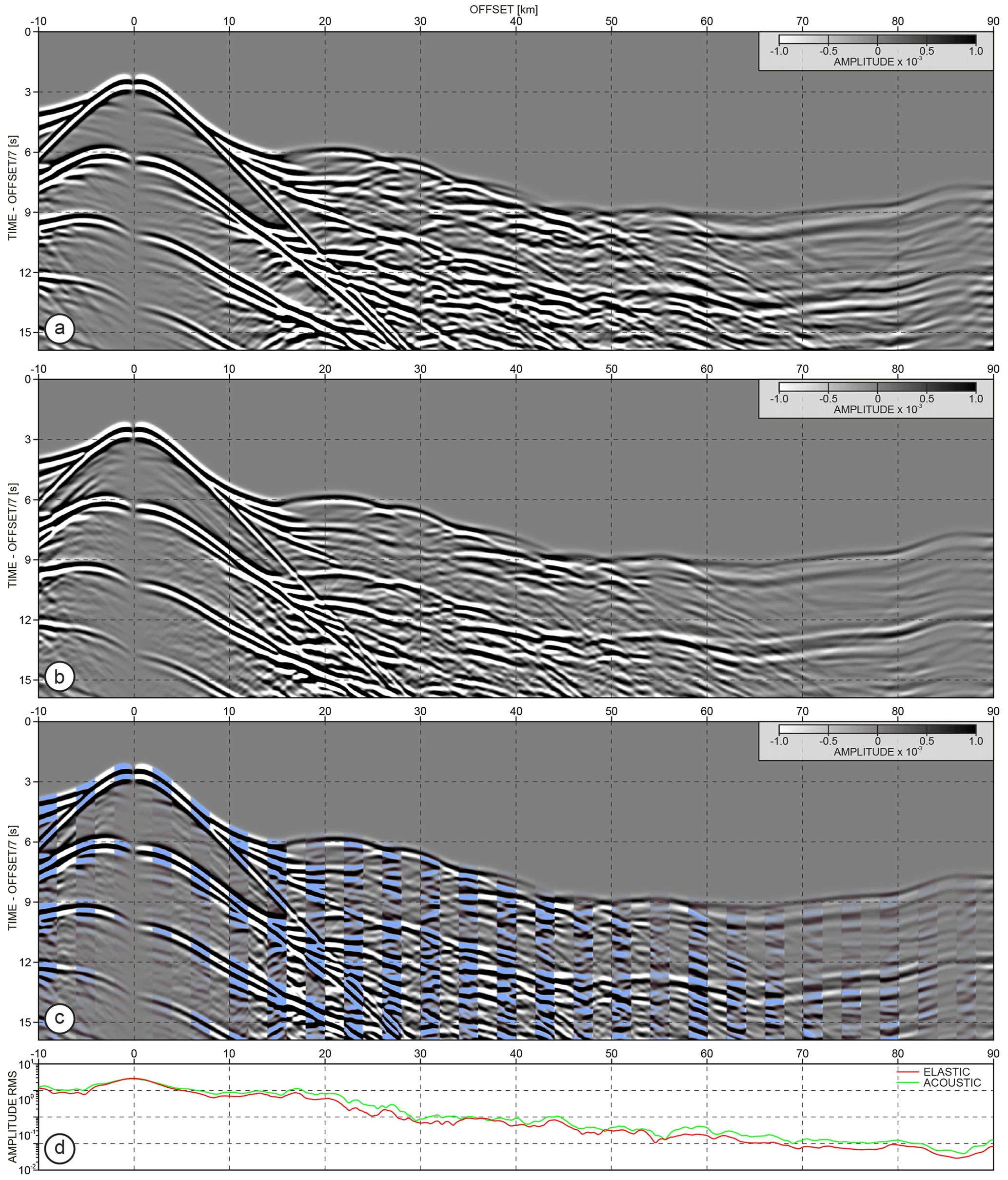
Figure 13OBS gathers generated using 3D spectral-element (a) acoustic and (b) elastic waveform modelling. (c) Comparison of seismograms from (a, b) where 20 traces from acoustic modelling (light-blue shading) are interleaved with the following 20 traces from the elastic equivalent. For better readability, the seismograms are scaled with the absolute offset value. (d) Rms amplitude curves of the gathers from (a, b) – without scaling with offset.
From the rms amplitude curves in Fig. 13d, we can see that the acoustic–elastic seismograms have generally lower amplitudes than the pure acoustic data. The trend of this difference, however, varies with offset (unlike, e.g., in Fig. 10d) indicating that the elastic effects are non-uniformly distributed along the offset intervals.
It is also worth to mention here, that the data simulated with the finite-difference scheme exhibit some evidence of so called “staircase effect” (see diffraction-like patterns in the short-offset data in Fig. 11a and b). These artefacts result from the bathymetry projection on the Cartesian grid (50 m grid step). In contrast, the spectral-element mesh can accurately handle the sharp seabed interface which is reflected by lack of similar artefacts in the gathers from Fig. 13.
4.1 Geological setting of GO_3D_OBS
Our previous studies oriented on crustal-scale seismic imaging from OBS data were located in the Tokai area of the Nankai Trough (Górszczyk et al., 2017, 2019). This gave us a true-earth reference to guide the building of a first version of our model. However, our primary aim was to build a structural model which involves as many as possible geological features observed in subduction zones rather than following rigorously the Nankai Trough geological setting. On this basis, the GO_3D_OBS shall be seen as a generic crustal-scale benchmark model of subduction zone rather than a seismological reference to the Tokai segment. We hope that in future, based on some feedback from the community, we will be able to incorporate more geological features or modify existing ones.
4.2 Acquisition design
In the academic community of marine geosciences, sparse OBS acquisitions remain the primary tool for offshore lithospheric model reconstruction. The acquisition-related issues focus mainly on the shooting strategy and the optimal OBS spacing (Brenders and Pratt, 2007a). This is the consequence of the fact that the number of available instruments is limited (∼100 maximum). The spacing between OBS must not be chosen at the expense of the maximum offset sampled by the acquisition, as this maximum offset should be enough to record diving waves that reach the deepest structures (namely the upper mantle). On the other hand, the sparse acquisition design shall minimize model distortions resulting from an incomplete structure illumination associated with limited coverage of the surface acquisition. These distortions need to be assessed since they can generate significant bias during geological interpretation.
To investigate the footprint of various acquisition settings on the imaged target, realistic synthetic models are necessary for the survey design. The processing of different datasets generated in such models would allow for the optimization of the acquisition setup to find the best compromise between deployment effort, image resolution, and target sampling. This was one of our main motivations behind the design of the GO_3D_OBS model. One of the ongoing projects now focuses on the investigations of the off-plane wavefield propagation during 2D crustal-scale FWI. From the modelling tests shown in this paper (Fig. 11), we can conclude that these effects may have a detrimental impact on the imaging results. This will stimulate the extension of routinely performed 2D OBS surveys toward the optimally designed future 3D deployments. We can evoke here the 2001 SFJ 2D OBS experiment (Operto et al., 2006), which was conducted in the Tokai area of the Nankai Trough using 100 OBS deployed with a dense 1 km spacing. Today, 3D sparse OBS deployments are conducted with a similar number of stations with an aim to apply FWI. Therefore, which of those two different acquisitions – dense 2D or sparse 3D – are closer to the optimal setting? Was the 2D SFJ profile oversampled or are today's 3D experiments maybe undersampled? Is it possible to solve (at least to a certain extent) the sparse OBS acquisition issues with more robust sparsity-promoting regularization techniques? Or maybe this undersampling can be solved by acquiring the coincident long-streamer data? If so, what would be the most efficient shooting strategy comprising both types of experiments? We believe that for a new FWI-optimized OBS surveys we should look for a justification of a proposed acquisition geometry rather than use an ad hoc configuration.
4.3 Usefulness for tomography
Although the processing method we pair the most with our model is FWI, there are no limits in terms of the application of other tomographic techniques, for example ray-theory-based modelling techniques such as ray-tracing or eikonal solvers. While FAT is typically producing rather smooth velocity models, the other variants of tomography have the potential to build models with improved resolution. An evaluation of those tomographic methods against GO_3D_OBS model can lead to their further development. Travel time tomography techniques are in general computationally much less intensive than waveform inversion methods. It is therefore worth pushing their efficiency to the resolution limits and validating them with complex benchmarks. This kind of development of tomographic methods indirectly contributes also to FWI popularization since the tomographic models are usually used as initial models for FWI.
4.4 Uncertainty estimation
Together with the development of different seismic imaging techniques, methods for the quantitative estimation of their uncertainty and resolution limits shall be proposed. Indeed, this subject is not trivial when facing real-data processing and therefore the issue is often skipped by authors. The obvious problem is that the true geological structure is never exactly known, and therefore the model of this structure has no direct reference point to compare. On the other hand, the resolution and accuracy of the seismic imaging methods are always limited. Therefore, it shall lead us to reflect on the potential pitfalls related to overinterpretations during real-data case studies.
Sparse OBS deployments combined with travel time tomography processing techniques lead to a wide range of similar smooth velocity models of the crust, which explain the travel time data equally well. In such a scenario, the Monte Carlo random sampling of the model space supported by the estimation of probability density of the model parameters (Korenaga and Sager, 2012) can reduce the null-space of the final models and make the geological interpretation more certain.
On the other hand, the high-resolution reconstruction methods relying on the inversion of the waveforms recorded by denser OBS acquisitions are also burdened with uncertainty. The fact that those techniques are waveform driven makes the reliability of the wavefield propagation simulation one of the key factors for the final model accuracy. The popular acoustic wavefield modelling and inversion can be precise enough for the overall reconstruction of the medium without, e.g., strong velocity contrasts, fluid-related attenuation zones, and anisotropic layers. However, in the case of the presence of such structures, the acoustic approximation can lead to significant reconstruction error in the final model. The significance of this error is poorly understood, and therefore the evaluation of the uncertainty of the inversion methods with realistic synthetic tests can bring us closer to the estimation of the error during real-data processing, not only because we know the underlying structure exactly but also because of the possibility of investigating the influence of different approximations, experiment geometries, or noise.
4.5 Further development
At the current stage of development, we believe that GO_3D_OBS is sufficiently realistic to explore the validity of various tomographic and inversion methods on synthetic datasets with different acquisition designs. Future branches of development of this benchmark can cover different aspects including both structural components and parameterization. For instance, one of the interesting topics is extension toward anisotropy. Building such an anisotropy model consistent with geological studies of the deep crust could be challenging due to the general difficulty of precise anisotropy estimation. Nevertheless, it would significantly increase the authenticity of the corresponding seismic data. On the other hand, generating an accompanying dataset for the current models can further broaden their impact. A possible dataset could include sparse 3D and dense 2D OBS deployments, as well as corresponding streamer data. Such a dataset could be directly used for a given type of processing. In particular, generating the seismic data without and with a realistic type and level of noise would help to further evaluate the impact of noise on the accuracy of the reconstruction of the final structure.
We developed the GO_3D_OBS reference geomodel for the purpose of assessing different crustal-scale seismic imaging methods, as well as for guiding various seismic acquisition designs. The 3D model structure allows for the extraction of sub-volumes representing a different level of complexity that can be found in subduction zone environments. The viscoelastic parameterization of the medium gives the potential user the possibility to assess the impact of various physical approximations during model reconstruction. There are various components influencing the current state of the art in terms of crustal-scale imaging. Among them, methodological developments aimed at computationally efficient seismic wave modelling engines and robust inversion schemes assessed against realistic large-scale problems significantly contribute to further exciting geological discoveries. From this perspective, we believe that our model will help to further stimulate high-resolution seismic imaging of the deep lithosphere and thus will help to understand the processes that shape the earth's crust.
The current version of the model and the user manual are available from the data repository of the Institute of Geophysics, Polish Academy of Sciences: https://dataportal.igf.edu.pl/dataset/go_3d_obs (last access: 24 March 2021, IG PAS Data Portal, 2021). All rights to the source code are reserved to the SEISCOPE consortium and the Institute of Geophysics, Polish Academy of Sciences. Information regarding the implementation are available upon request from the corresponding author.
AG and SO initiated the research and setup the overall concept of the 3D model. AG designed and implemented the workflow for building the model structure, the physical parameterization, and the stochastic components. SO validated each of the model ingredients. AG designed and performed seismic modelling simulations. AG prepared the initial version of the paper, which was further updated toward the final version with the contribution from SO.
The authors declare that they have no conflict of interest.
This study was partially funded by (i) the SEISCOPE consortium (http://seiscope2.osug.fr, last access: 16 March 2021), sponsored by AKERBP, CGG, CHEVRON, EQUINOR, EXXON-MOBIL, JGI, SHELL, SINOPEC, SISPROBE, and TOTAL and (ii) the Polish National Science Center (grant no: 2019/33/B/ST10/01014). The study was granted access to the HPC PL-Grid Infrastructure (grant ID: 3dwind and 3dwind2). We thank Romain Brossier and Jian Cao for their support of this study through the development of the TOYXDAC and SEM46 codes, as well as Ludovic Metivier and Jean Virieux for the internal review of the paper. We thank the geological community from the Geoazur and JAMSTEC institutes for their feedback which allowed us to improve the structure of our model.
This research has been supported by the Polish National Science Center and the SEISCOPE consortium.
This paper was edited by Rolf Sander and reviewed by Rie Nakata and one anonymous referee.
Agard, P., Plunder, A., Angiboust, S., Bonnet, G., and Ruh, J.: The subduction plate interface: rock record and mechanical coupling (from long to short timescales), Lithos, 320–321, 537–566, https://doi.org/10.1016/j.lithos.2018.09.029, 2018. a
Aghamiry, H., Gholami, A., and Operto, S.: Improving full-waveform inversion by wavefield reconstruction with alternating direction method of multipliers, Geophysics, 84, R139–R162, 2019a. a
Aghamiry, H., Gholami, A., and Operto, S.: On the robustness of ℓ1-regularized ADMM-based wavefield reconstruction inversion against compressed acquisition sampling, SEG Technical Program Expanded Abstracts, 1385–1389, 2019b. a
Agudelo, W., Ribodetti, A., Collot, J.-Y., and Operto, S.: Joint inversion of multichannel seismic reflection and wide-angle seismic data: Improved imaging and refined velocity model of the crustal structure of the north Ecuador–south Colombia convergent margin, J. Geophys. Res., 114, B02306, https://doi.org/10.1029/2008JB005690, 2009. a
Aminzadeh, F., Brac, J., and Kunz, T.: SEG/EAGE 3-D Salt and Overthrust Models. SEG/EAGE 3-D Modeling Series, No. 1: Distribution CD of Salt and Overthrust models, SEG book series, 1997. a
Angiboust, S., Glodny, J., Oncken, O., and Chopin, C.: In search of transient subduction interfaces in the Dent Blanche-Sesia Tectonic System (W. Alps), Lithos, 205, 298–321, https://doi.org/10.1016/j.lithos.2014.07.001, 2014. a
Angiboust, S., Agard, P., Glodny, J., Omrani, J., and Oncken, O.: Zagros blueschists: Episodic underplating and long-lived cooling of a subduction zone, Earth Planet. Sci. Lett., 443, 48–58, https://doi.org/10.1016/j.epsl.2016.03.017, 2016. a
Arai, R., Kodaira, S., Henrys, S. A., Bangs, N. L., Obana, K., Fujie, G., Miura, S., Barker, D. H. N., Bassett, D., Bell, R. E., Morgan, J. V., Warner, M., Mochizuki, K., Kellett, R. L., Stucker, V., and Fry, B.: Three-dimensional anisotropic P-wave velocity structure around the shallow plate boundary in the Northern Hikurangi margin, New Zealand, AGU Fall Meeting 2019, San Francisco, USA, 9–13 December 2019, T51F–0357, 2019. a
Azuma, S., Yamamoto, S., Ichikawa, H., and Maruyama, S.: Why primordial continents were recycled to the deep: Role of subduction erosion, Geosci. Front., 8, 337–346, https://doi.org/10.1016/j.gsf.2016.08.001, 2017. a
Bangs, N., Moore, G., Gulick, S., Pangborn, E., Tobin, H., Kuramoto, S., and Taira, A.: Broad, weak regions of the Nankai Megathrust and implications for shallow coseismic slip, Earth Planet. Sci. Lett., 284, 44–49, https://doi.org/10.1016/j.epsl.2009.04.026, 2009. a
Bauer, A., Schwarz, B., and Gajewski, D.: Utilizing diffractions in wavefront tomography, Geophysics, 82, R65–R73, 2017. a
Ben-Zion, Y. and Sammis, C. G.: Characterization of fault zones, Pure Appl. Geophys., 160, 677–715, 2003. a, b
Billette, F., Podvin, P., and Lambaré, G.: Stereotomography with automatic picking: application to the Marmousi dataset, SEG Technical Program Expanded Abstracts 1998, II, 1317–1320, https://doi.org/10.1190/1.1820143, 1998. a
Billette, F. J. and Brandsberg-Dahl, S.: The 2004 BP Velocity Benchmark, in: Extended Abstracts, 67th Annual EAGE Conference & Exhibition, Madrid, Spain, 13–16 June 2005, B035, 2004. a
Bishop, T. N., Bube, K. P., Cutler, R. T., Langan, R. T., Love, P. L., Resnick, J. R., Shuey, R. T., and Spinder, D. A.: Tomographic determination of velocity and depth in laterally varying media, Geophysics, 50, 903–923, 1985. a
Blanch, J., Jarvis, J., Hurren, C., Liu, Y., and Hu, L.: Designing an exploration scale OBN: Acquisition design for subsalt imaging and velocity determination, SEG Technical Program Expanded Abstracts: 192–196, 2019. a
Boston, B., Moore, G. F., Nakamura, Y., and Kodaira, S.: Outer-rise normal fault development and influence on near-trench décollement propagation along the Japan Trench, off Tohoku, Earth Planet. Space, 66, 135, https://doi.org/10.1186/1880-5981-66-135, 2014. a
Brenders, A. J. and Pratt, R. G.: Efficient waveform tomography for lithospheric imaging: implications for realistic 2D acquisition geometries and low frequency data, Geophys. J. Int., 168, 152–170, 2007a. a, b
Brenders, A. J. and Pratt, R. G.: Full waveform tomography for lithospheric imaging: results from a blind test in a realistic crustal model, Geophys. J. Int., 168, 133–151, 2007b. a
Brocher, T. M.: Empirical relationships between elastic wavespeeds and density in the earth's crust, B. Seismol. Soc. Am., 95, 2081–2092, 2005. a, b, c
Brossier, R., Operto, S., and Virieux, J.: Velocity model building from seismic reflection data by full waveform inversion, Geophys. Prospect., 63, 354–367, https://doi.org/10.1111/1365-2478.12190, 2015. a
Cawood, P. A., Kröner, A., Collins, W. J., Kusky, T. M., Mooney, W. D., and Windley, B. F.: Accretionary orogens through Earth history, Geol. Soc. Spec. Pub., 318, 1–36, https://doi.org/10.1144/sp318.1, 2009. a
Christensen, N. I. and Mooney, W. D.: Seismic velocity structure and composition of the continental crust: a global view, J. Geophys. Res., 100, 9761–9788, 1995. a
Claerbout, J. F.: Imaging the Earth's interior, Blackwell Scientific Publication, Oxford, 414 pp., 1985. a
Collot, J.-Y., Agudelo, W., Ribodetti, A., and Marcaillou, B.: Origin of a crustal splay fault and its relation to the seismogenic zone and underplating at the erosional north Ecuador–south Colombia oceanic margin, J. Geophys. Res., 113, B12102, https://doi.org/10.1029/2008jb005691, 2008. a, b
Collot, J.-Y., Ribodetti, A., Agudelo, W., and Sage, F.: The South Ecuador subduction channel: Evidence for a dynamic mega-shear zone from 2D fine-scale seismic reflection imaging and implications for material transfer, J. Geophys. Res., 116, B11102, https://doi.org/10.1029/2011jb008429, 2011. a
Contreras-Reyes, E., Flueh, E. R., and Grevemeyer, I.: Tectonic control on sediment accretion and subduction off south central Chile: Implications for coseismic rupture processes of the 1960 and 2010 megathrust earthquakes, Tectonics, 29, TC6018, https://doi.org/10.1029/2010tc002734, 2010. a
Dessa, J.-X., Operto, S., Kodaira, S., Nakanishi, A., Pascal, G., Uhira, K., and Kaneda, Y.: Deep seismic imaging of the eastern Nankai trough (Japan) from multifold ocean bottom seismometer data by combined traveltime tomography and prestack depth migration, J. Geophys. Res., 109, B02111, https://doi.org/10.1029/2003JB002689, 2004. a, b
Ducea, M. N. and Chapman, A. D.: Sub-magmatic arc underplating by trench and forearc materials in shallow subduction systems; A geologic perspective and implications, Earth-Sci. Rev., 185, 763–779, https://doi.org/10.1016/j.earscirev.2018.08.001, 2018. a
Farra, V. and Madariaga, R.: Non-linear reflection tomography, Geophys. J., 95, 135–147, 1988. a
Goff, J. A. and Holliger, K.: Heterogeneity in the Crust and Upper Mantle, Springer US, Springer, Boston, MA, https://doi.org/10.1007/978-1-4615-0103-9, 2003. a
Goncharov, A., Cooper, A., Chia, P., and O'Neil, P.: A new dawn for Australian ocean-bottom seismography, Leading Edge, 35, 99–104, https://doi.org/10.1190/tle35010099.1, 2016. a
Górszczyk, A. and Operto, S.: GO_3D_OBS – The multi-parameter benchmark geomodel for seismic imaging methods assessment and next generation 3D surveys design (version 1.0), IG PAS Data Portal, https://doi.org/10.25171/InstGeoph_PAS_IGData-NCN36-2020-001, 2020.
Górszczyk, A., Operto, S., and Malinowski, M.: Toward a robust workflow for deep crustal imaging by FWI of OBS data: The eastern Nankai Trough revisited, J. Geophys. Res-Sol. Ea., 122, 4601–4630, https://doi.org/10.1002/2016jb013891, 2017. a, b, c, d, e, f
Górszczyk, A., Operto, S., Schenini, L., and Yamada, Y.: Crustal-scale depth imaging via joint full-waveform inversion of ocean-bottom seismometer data and pre-stack depth migration of multichannel seismic data: a case study from the eastern Nankai Trough, Solid Earth, 10, 765–784, https://doi.org/10.5194/se-10-765-2019, 2019. a, b, c, d
Gras, C., Dagnino, D., Jiménez-Tejero, C. E., Meléndez, A., Sallarès, V., and Ranero, C. R.: Full-waveform inversion of short-offset, band-limited seismic data in the Alboran Basin (SE Iberia), Solid Earth, 10, 1833–1855, https://doi.org/10.5194/se-10-1833-2019, 2019. a
Gutscher, M.-A., Kukowski, N., Malavieille, J., and Lallemand, S.: Cyclical behavior of thrust wedges: Insights from high basal friction sandbox experiments, Geology, 24, 135–138, https://doi.org/10.1130/0091-7613(1996)024<0135:cbotwi>2.3.co;2, 1996. a
Gutscher, M.-A., Kukowski, N., Malavieille, J., and Lallemand, S.: Material transfer in accretionary wedges from analysis of a systematic series of analog experiments, J. Struct. Geol., 20, 407–416, https://doi.org/10.1016/s0191-8141(97)00096-5, 1998. a
Hale, D.: Dynamic warping of seismic images, Geophysics, 78, S105–S115, 2013. a, b
Hashimoto, Y. and Kimura, G.: Underplating process from melange formation to duplexing: Example from the Cretaceous Shimanto Belt, Kii Peninsula, southwest Japan, Tectonics, 18, 92–107, https://doi.org/10.1029/1998tc900014, 1999. a
Heath, B. A., Hooft, E. E. E., Toomey, D. R., Papazachos, C. B., Nomikou, P., Paulatto, M., Morgan, J. V., and Warner, M. R.: Tectonism and Its Relation to Magmatism Around Santorini Volcano From Upper Crustal P Wave Velocity, J. Geophys. Res.-Sol. Ea., 124, 10610–10629, https://doi.org/10.1029/2019jb017699, 2019. a
Herrmann, F. J.: Randomized sampling and sparsity: Getting more information from fewer samples, Geophysics, 75, WB173–WB187, 2010. a
Hole, J. A., Zelt, C. A., and Pratt, R. G.: Advances in controlled-source seismic imaging, Eos T. Am. Geophys. Un., 86, 177–184, 2005. a
Holliger, K., Levander, A. R., and Goff, J. A.: Stochastic modeling of the reflective lower crust: petrophysical and geological evidence from the Ivrea zone (Northern Italy), J. Geophys. Res., 98, 11967–11980, 1993. a
Huang, L. and Liu, C.-y.: Three Types of Flower Structures in a Divergent-Wrench Fault Zone, J. Geophys. Res.-Sol. Ea., 122, 10478–10497, https://doi.org/10.1002/2017JB014675, 2017. a
IG PAS Data Portal, https://dataportal.igf.edu.pl/dataset/go_3d_obs, last access: 24 March 2021. a
Jannane, M., Beydoun, W., Crase, E., Cao, D., Koren, Z., Landa, E., Mendes, M., Pica, A., Noble, M., Roeth, G., Singh, S., Snieder, R., Tarantola, A., and Trezeguet, D.: Wavelengths of Earth structures that can be resolved from seismic reflection data, Geophysics, 54, 906–910, 1989. a
Kameda, J., Inoue, S., Tanikawa, W., Yamaguchi, A., Hamada, Y., Hashimoto, Y., and Kimura, G.: Alteration and dehydration of subducting oceanic crust within subduction zones: implications for décollement step-down and plate-boundary seismogenesis, Earth Planet. Space, 69, 52, https://doi.org/10.1186/s40623-017-0635-1, 2017. a
Kamei, R., Pratt, R. G., and Tsuji, T.: Waveform tomography imaging of a megasplay fault system in the seismogenic Nankai subduction zone, Earth Planet. Sci. Lett., 317–318, 343–353, 2012. a, b
Kamei, R., Pratt, R. G., and Tsuji, T.: On acoustic waveform tomography of wide-angle OBS data – Strategies for preconditioning and inversion, Geophys. J. Int., 192, 1250–1280, 2013. a
Kington, J.: The Structure and Kinematics of the Nankai Trough Accretionary Prism, Japan, PhD thesis, University of Wisconsin-Madison, 2012. a, b
Kington, J. D. and Tobin, H. J.: Balanced Cross Sections, Shortening Estimates, and the Magnitude of Out-of-Sequence Thrusting in the Nankai Trough Accretionary Prism, Japan, AGU Fall Meeting 2011, San Francisco, USA, 5–9 December 2011, T21B–2364, 2011. a
Kodaira, S.: Subducted Seamount Imaged in the Rupture Zone of the 1946 Nankaido Earthquake, Science, 289, 104–106, https://doi.org/10.1126/science.289.5476.104, 2000. a
Kodaira, S., Kurashimo, E., Park, J.-O., Takahashi, N., Nakanishi, A., Miura, S., Iwasaki, T., Hirata, N., Ito, K., and Kaneda, Y.: Structural factors controlling the rupture process of a megathrust earthquake at the Nankai trough seismogenic zone, Geophys. J. Int., 149, 815–835, 2002. a, b
Kodaira, S., Nakanishi, A., Park, J. O., Ito, A., Tsuru, T., and Kaneda, Y.: Cyclic ridge subduction at an inter-plate locked zone off Central Japan, Geophys. Res. Lett., 30, 1339, https://doi.org/10.1029/2002GL016595, 2003. a
Korenaga, J. and Sager, W. W.: Seismic tomography of Shatsky Rise by adaptive importance sampling, J. Geophys. Res., 117, B08102, https://doi.org/10.1029/2012jb009248, 2012. a
Korenaga, J., Holbrook, W. S., Kent, G. M., Kelemen, P. B., Detrick, R. S., Larsen, H. C., Hopper, J. R., and Dahl-Jensen, T.: Crustal structure of the southeast Greenland margin from joint refraction and reflection seismic tomography, J. Geophys. Res., 105, 21591–21614, 2000. a
Lallemand, S., Mallavieille, J., and Calassou, S.: Effects of ridge oceanic subduction on accretionary wedges: Experimental modeling and marine observations, Tectonics, 11, 1301–1313, 1992. a
Lallemant, S., Chamot-Rooke, N., Le Pichon, X., and Rangin, C.: Zenisu ridge: a deep intraoceanic thrust related to subduction, off Southwest Japan, Tectonophysics, 160, 151–174, 1989. a
Lambaré, G.: Stereotomography, Geophysics, 73, VE25–VE34, 2008. a
Le Pichon, X., Lallemant, S., Tokuyama, H., Thoué, F., Huchon, P., and Henry, P.: Structure and evolution of the backstop in the eastern Nankai trough area (Japan): immplicationsn for the soon-to-come Tokai earthquake, Island Arc, 5, 440–454, 1996. a
Li, Q., Slopey, W., Rollins, F., Billette, F., Udengaard, C., and Thompson, B.: Leading a new deep water OBN acquisition era: Two 2017-2018 GoM OBN surveys, SEG Technical Program Expanded Abstracts 2019, 187–191, https://doi.org/10.1190/segam2019-3216437.1, 2019. a, b
Li, Y.-G. and Malin, P. E.: San Andreas Fault damage at SAFOD viewed with fault-guided waves, Geophys. Res. Lett., 35, L08304, https://doi.org/10.1029/2007gl032924, 2008. a
Lin, L.-F., Hsu, H.-H., Liu, C.-S., Chao, K.-H., Ko, C.-C., Chiu, S.-D., Hsieh, H.-S., Ma, Y.-F., and Chen, S.-C.: Marine 3D seismic volumes from 2D seismic survey with large streamer feathering, Mar. Geophys. Res., 40, 619–633, https://doi.org/10.1007/s11001-019-09391-9, 2019. a
Luo, Y. and Schuster, G. T.: Wave-equation traveltime inversion, Geophysics, 56, 645–653, 1991. a
Marjanović, M., Plessix, R.-É., Stopin, A., and Singh, S. C.: Elastic versus acoustic 3-D Full Waveform Inversion at the East Pacific Rise 9∘50′ N, Geophys. J. Int., 216, 1497–1506, https://doi.org/10.1093/gji/ggy503, 2018. a
Mei, J., Zhang, Z., Lin, F., Huang, R., Wang, P., and Mifflin, C.: Sparse nodes for velocity: Learnings from Atlantis OBN full-waveform inversion test, SEG Technical Program Expanded Abstracts 2019, 167–171, https://doi.org/10.1190/segam2019-3215208.1, 2019. a
Meléndez, A., Korenaga, J., Sallarès, V., Miniussi, A., and Ranero, C.: TOMO3D: 3-D joint refraction and reflection traveltime tomography parallel code for active-source seismic data-synthetic test, Geophys. J. Int., 203, 158–174, https://doi.org/10.1093/gji/ggv292, 2015. a
Menant, A., Angiboust, S., Monié, P., Oncken, O., and Guigner, J.-M.: Brittle deformation during Alpine basal accretion and the origin of seismicity nests above the subduction interface, Earth Planet. Sci. Lett., 487, 84–93, https://doi.org/10.1016/j.epsl.2018.01.029, 2018. a
Mercerat, E. D. and Nolet, G.: On the linearity of cross-correlation delay times in finite-frequency tomography, Geophys. J. Int., 192, 681–687, 2013. a
Métivier, L., Allain, A., Brossier, R., Mérigot, Q., Oudet, E., and Virieux, J.: Optimal transport for mitigating cycle skipping in full waveform inversion: a graph space transform approach, Geophysics, 83, R515–R540, https://doi.org/10.1190/geo2017-0807.1, 2018. a
Miller, D., Oristaglio, M., and Beylkin, G.: A new slant on seismic imaging: Migration and integral geometry, Geophysics, 52, 943–964, 1987. a
Mooney, W. D., Laske, G., and Masters, G.: CRUST 5.1: a global crustal model at 5∘ × 5∘, J. Geophys. Res., 103, 727–747, 1998. a
Mora, P. R.: Elastic wavefield inversion of reflection and transmission data, Geophysics, 53, 750–759, 1988. a
Morgan, J., Warner, M., Bell, R., Ashley, J., Barnes, D., Little, R., Roele, K., and Jones, C.: Next-generation seismic experiments: wide-angle, multi-azimuth, three-dimensional, full-waveform inversion, Geophys. J. Int., 195, 1657–1678, 2013. a
Morgan, J., Warner, M., Arnoux, G., Hooft, E., Toomey, D., VanderBeek, B., and Wilcock, W.: Next-generation seismic experiments – II: wide-angle, multi-azimuth, 3-D, full-waveform inversion of sparse field data, Geophys. J. Int., 204, 1342–1363, 2016. a
Neves, F. A. and Singh, S. C.: Sensitivity study of seismic reflection/refraction data, Geophys. J. Int., 126, 470–476, 1996. a
Ni, D., Brenders, A., Dellinger, J., van Gestel, J.-P., and Li, Q.: Seismic modeling for a velocity survey at Atlantis, SEG Technical Program Expanded Abstracts 2019, 182–186, https://doi.org/10.1190/segam2019-3215801.1, 2019. a
Olsen, K., Day, S., and Bradley, C.: Estimation of Q for long-period (>2 sec) waves in the Los Angeles basin, B. Seismol. Soc. Am., 93, 627–638, 2003. a, b
Operto, S., Virieux, J., Dessa, J. X., and Pascal, G.: Crustal imaging from multifold ocean bottom seismometers data by frequency-domain full-waveform tomography: application to the eastern Nankai trough, J. Geophys. Res., 111, B09306, https://doi.org/10.1029/2005JB003835, 2006. a, b
Operto, S., Miniussi, A., Brossier, R., Combe, L., Métivier, L., Monteiller, V., Ribodetti, A., and Virieux, J.: Efficient 3-D frequency-domain mono-parameter full-waveform inversion of ocean-bottom cable data: application to Valhall in the visco-acoustic vertical transverse isotropic approximation, Geophys. J. Int., 202, 1362–1391, 2015. a
Pangman, P.: SEAM launched in March, Leading Edge, 26, 718–720, https://doi.org/10.1190/tle26060718.1, 2007. a
Park, J. O., Moore, G. F., Tsuru, T., Kodaira, S., and Kaneda, Y.: A subducted oceanic ridge influencing the Nankai megathrust earthquake rupture, Earth Planet. Sci. Lett., 217, 77–84, 2004. a
Park, J. O., Fujie, G., Wijerathne, L., Hori, T., Kodaira, S., Fukao, Y., Moore, G. F., Bangs, N. L., Kuramoto, S., and Taira, A.: A low-velocity zone with weak reflectivity along the Nankai subduction zone, Geology, 38, 283–286, 2010. a
Pozgay, S. H., Wiens, D. A., Conder, J. A., Shiobara, H., and Sugioka, H.: Seismic attenuation tomography of the Mariana subduction system: Implications for thermal structure, volatile distribution, and slow spreading dynamics, Geochem. Geophy. Geosy., 10, Q04X05, https://doi.org/10.1029/2008gc002313, 2009. a
Pratt, R. G.: Waveform tomography – successes, cautionary tales, and future directions, in: Presented at the 70th Annual EAGE Conference and Exhibition, Roma, 9–12 June 2008, WO11, 2008. a
Pratt, R. G., Song, Z. M., Williamson, P. R., and Warner, M.: Two-dimensional velocity models from wide-angle seismic data by wavefield inversion, Geophys. J. Int., 124, 323–340, 1996. a
Qin, Y. and Singh, S. C.: Detailed seismic velocity of the incoming subducting sediments in the 2004 great Sumatra earthquake rupture zone from full waveform inversion of long offset seismic data, Geophys. Res. Lett., 44, 3090–3099, https://doi.org/10.1002/2016gl072175, 2017. a
Raimbourg, H., Augier, R., Famin, V., Gadenne, L., Palazzin, G., Yamaguchi, A., and Kimura, G.: Long-term evolution of an accretionary prism: The case study of the Shimanto Belt, Kyushu, Japan, Tectonics, 33, 936–959, https://doi.org/10.1002/2013tc003412, 2014. a
Ranero, C. R., Villaseñor, A., Morgan, J. P., and Weinrebe, W.: Relationship between bend-faulting at trenches and intermediate-depth seismicity, Geochem. Geophy. Geosy., 6, Q12002, https://doi.org/10.1029/2005gc000997, 2005. a
Ribodetti, A., Operto, S., Agudelo, W., Collot, J.-Y., and Virieux, J.: Joint ray + Born least-squares migration and simulated annealing optimization for high-resolution target-oriented quantitative seismic imaging, Geophysics, 76, R23–R42, 2011. a
Ross, M. R., Sprague, M. A., Felippa, C. A., and Park, K. C.: Treatment of acoustic fluid-structure interaction by localized Lagrange multipliers and comparison to alternative interface-coupling methods, Comput. Method. Appl. M., 198, 986–1005, 2009. a
Sambolian, S., Operto, S., Ribodetti, A., Tavakoli, B., and Virieux, J.: Parsimonious slope tomography based on eikonal solvers and the adjoint-state method, Geophys. J. Int., 218, 456–478, https://doi.org/10.1093/gji/ggz150, 2019. a
Shipp, R. M. and Singh, S. C.: Two-dimensional full wavefield inversion of wide-aperture marine seismic streamer data, Geophys. J. Int., 151, 325–344, 2002. a
Shiraishi, K., Moore, G. F., Yamada, Y., Kinoshita, M., Sanada, Y., and Kimura, G.: Seismogenic zone structures revealed by improved 3D seismic images in the Nankai Trough off Kumano, Geochem. Geophy. Geosy., 20, 2252–2271, https://doi.org/10.1029/2018gc008173, 2019. a
Sirgue, L. and Pratt, R. G.: Efficient waveform inversion and imaging: a strategy for selecting temporal frequencies, Geophysics, 69, 231–248, 2004. a
Tarantola, A.: Inversion of seismic reflection data in the acoustic approximation, Geophysics, 49, 1259–1266, 1984. a
Tavakoli F., B., Operto, S., Ribodetti, A., and Virieux, J.: Slope tomography based on eikonal solvers and the adjoint-state method, Geophys. J. Int., 209, 1629–1647, 2017. a
Tavakoli F., B., Operto, S., Ribodetti, A., and Virieux, J.: Matrix-free anisotropic slope tomography: theory and application, Geophysics, 84, R35–R57, 2019. a
Tong, P., Zhao, D., Yang, D., Yang, X., Chen, J., and Liu, Q.: Wave-equation-based travel-time seismic tomography – Part 1: Method, Solid Earth, 5, 1151–1168, https://doi.org/10.5194/se-5-1151-2014, 2014. a
Tsuji, T., Kodaira, S., Ashi, J., and Park, J.-O.: Widely distributed thrust and strike-slip faults within subducting oceanic crust in the Nankai Trough off the Kii Peninsula, Japan, Tectonophysics, 600, 52–62, 2013. a
Tsuji, T., Ashi, J., and Ikeda, Y.: Strike-slip motion of a mega-splay fault system in the Nankai oblique subduction zone, Earth Planet. Space, 66, 120, https://doi.org/10.1186/1880-5981-66-120, 2014. a
Tsuji, T., Minato, S., Kamei, R., Tsuru, T., and Kimura, G.: 3D geometry of a plate boundary fault related to the 2016 Off-Mie earthquake in the Nankai subduction zone, Japan, Earth Planet. Sci. Lett., 478, 234–244, https://doi.org/10.1016/j.epsl.2017.08.041, 2017. a
van Leeuwen, T. and Herrmann, F. J.: Mitigating local minima in full-waveform inversion by expanding the search space, Geophys. J. Int., 195, 661–667, https://doi.org/10.1093/gji/ggt258, 2013. a
Vannucchi, P., Sage, F., Morgan, J. P., Remitti, F., and Collot, J.-Y.: Toward a dynamic concept of the subduction channel at erosive convergent margins with implications for interplate material transfer, Geochem. Geophy. Geosy., 13, Q02003, https://doi.org/10.1029/2011gc003846, 2012. a
Versteeg, R.: The Marmousi experience: Velocity model determination on a synthetic complex data set, Leading Edge, 13, 927–936, https://doi.org/10.1190/1.1437051, 1994. a
Virieux, J. and Operto, S.: An overview of full waveform inversion in exploration geophysics, Geophysics, 74, WCC1–WCC26, 2009. a
von Huene, R., Ranero, C. R., and Vannucchi, P.: Generic model of subduction erosion, Geology, 32, 913–916, https://doi.org/10.1130/g20563.1, 2004. a
Warner, M. and Guasch, L.: Adaptive waveform inversion: Theory, Geophysics, 81, R429–R445, 2016. a
Wellmann, F. and Caumon, G.: 3-D Structural geological models: Concepts, methods, and uncertainties, Adv. Geophys., 59, 1–121, https://doi.org/10.1016/bs.agph.2018.09.001, 2018. a
Wiggens, R. A., Frazier, G. A., Sweet, J., and Apsel, R.: Modeling strong motions from major earthquakes, in: Proc. of the Second International Conference on Microzonation for Safer Construction: Research and Application, San Francisco, California, USA, 26 November–1 December 1978, 693–700, 1978. a, b
Wu, R. S. and Toksöz, M. N.: Diffraction tomography and multisource holography applied to seismic imaging, Geophysics, 52, 11–25, 1987. a
Wu, Z. and Alkhalifah, T.: Simultaneous inversion of the background velocity and the perturbation in full-waveform inversion, Geophysics, 80, R317–R329, 2015. a
Xu, S., Wang, D., Chen, F., Lambaré, G., and Zhang, Y.: Inversion on Reflected Seismic Wave, SEG Technical Program Expanded Abstracts 2012, 1–7, https://doi.org/10.1190/segam2012-1473.1, 2012. a
Yang, P., Brossier, R., Métivier, L., and Virieux, J.: A review on the systematic formulation of 3D multiparameter full waveform inversion in viscoelastic medium, Geophys. J. Int., 207, 129–149, https://doi.org/10.1093/gji/ggw262, 2016. a
Zelt, C. and Barton, P. J.: Three-dimensional seismic refraction tomography: a comparison of two methods applied to data from the Faeroe Basin, J. Geophys. Res., 103, 7187–7210, 1998. a
Zelt, C. A. and Chen, J.: Frequency-dependent traveltime tomography for near-surface seismic refraction data, Geophys. J. Int., 207, 72–88, 2016. a
Zhang, Z. and Stewart, R. R.: Seismic attenuation and well log analysis in a heavy oilfield, SEG Technical Program Expanded Abstracts 2008, 1784–1788, https://doi.org/10.1190/1.3059251, 2008. a, b
Zhou, W., Brossier, R., Operto, S., and Virieux, J.: Full Waveform Inversion of Diving & Reflected Waves for Velocity Model Building with Impedance Inversion Based on Scale Separation, Geophys. J. Int., 202, 1535–1554, 2015. a