Evaluation of ECMWF IFS-AER (CAMS) operational forecasts during cycle 41r1–46r1 with calibrated ceilometer profiles over Germany

Aerosol forecasts by the European Centre for Medium-Range Weather Forecasts (ECMWF) Integrated Forecasting System aerosol module (IFS-AER) for the years 2016–2019 (cycles 41r1–46r1) are compared to vertical profiles of particle backscatter from the Deutscher Wetterdienst (DWD) ceilometer network. The system has been developed in the Copernicus Atmosphere Monitoring Service (CAMS) and its precursors. The focus of this article is to evaluate the realism of the vertical aerosol distribution from 0.4 to 8 km above ground, coded in the shape, bias and temporal variation of the profiles. The common physical quantity, the attenuated backscatter β^∗(z), is directly measured and calculated from the model mass mixing ratios of the different particle types using the model's inherent aerosol microphysical properties.

Pearson correlation coefficients of daily average simulated and observed vertical profiles between r=0.6–0.8 in summer and 0.7–0.95 in winter indicate that most of the vertical structure is captured. It is governed by larger β^∗(z) in the mixing layer and comparably well captured with the successive model versions. The aerosol load tends to be biased high near the surface, underestimated in the mixing layer and realistic at small background values in the undisturbed free troposphere. A seasonal cycle of the bias below 1 km height indicates that aerosol sources and/or lifetimes are overestimated in summer and pollution episodes are not fully resolved in winter. Long-range transport of Saharan dust or fire smoke is captured and timely, only the dispersion to smaller scales is not resolved in detail. Over Germany, β^∗(z) values from Saharan dust and sea salt are considerably overestimated. Differences between model and ceilometer profiles are investigated using observed in situ mass concentrations of organic matter (OM), black carbon, SO₄, NO₃, NH₄ and proxies for mineral dust and sea salt near the surface. Accordingly, SO₄ and OM sources as well as gas-to-particle partitioning of the NO₃–NH₄ system are too strong. The top of the mixing layer on average appears too smooth and several hundred meters too low in the model. Finally, a discussion is included of the considerable uncertainties in the observations as well as the conversion from modeled to observed physical quantities and from necessary adaptions of varying resolutions and definitions.

1 Introduction

Aerosol particles play a key role in atmospheric processes, and their manifold sources and transformations reflect in a wide range of abundance as well as chemical and physical properties. Thus, the understanding of particles' net effects on air quality, weather, climate and chemical budgets still comprises significant uncertainties (Linares et al., 2009; WMO, 2013; Baklanov et al., 2014). Particles affect climate and weather directly by light scattering and absorption (Hansen et al., 1997; Ramanathan et al., 2007; WMO, 2013) and indirectly by altering the formation and droplet size of clouds (Lohmann et al., 2007) and via their impact on saturation and vertical exchange (Ackerman et al., 2000). Due to land-use changes and increasing emissions of anthropogenic gases and particles during the last century, aerosols constitute and trigger severe pollution episodes and health hazards (Galanter et al., 2000; Andreae and Merlet, 2001; Pérez et al., 2012). In the lower troposphere, particle emissions and heterogeneous chemical processes degrade health-related air quality (Gilge et al., 2010; Karanasiou et al., 2012), but at the same time particles mediate gas-to-particle conversion, scavenging and final removal of trace gases from the atmosphere (Birmili et al., 2003; Kolb and et al, 2010).

Natural particle sources, too, dependent on season, weather and region, may cause widespread socio-economical and epidemiological impacts. Europe, for example, is reached by Saharan dust (SD) many times per year (Ansmann and et al, 2003; Collaud-Coen et al., 2004; Papayannis et al., 2008; Pey et al., 2013; Flentje et al., 2015) where, decreasing towards the north, it contributes between 5 %–30 % to the total dry particle mass (Putaud et al., 2010). It triggers cloud formation (Sassen et al., 2003; Lohmann et al., 2007; Tegen and Schepanski, 2009) and summer smog (Ordonez et al., 2010; Wang, 2010) and has been associated with dispersion of bacteria like meningitis (Griffin, 2007; Karanasiou et al., 2012). Volcanic eruptions may induce long-term changes of radiation transfer (Jäger, 2005), disturb flight traffic (Flentje et al., 2010a; Schumann et al., 2011) and habitability of adjacent regions and alter the chemical balance up to the stratosphere. Domestic heating and open fires linked to agriculture (∼ 85 % globally; Andreae and Merlet, 2001), drought or boreal burns (Damoah et al., 2004; Hyer et al., 2007; Stohl et al., 2002) produce small-sized carbonaceous particles which can be widely distributed and may penetrate deep into lungs and plant stomata (Kaiser et al., 2012). Their fractal surfaces favor adsorption of harmful combustion byproducts that may cause respiratory, allergic, cardiovascular and cancerous diseases (Mölter et al., 2014).

Air-quality regulations like European directive 2008/50/EG for PM₁₀ $/$ PM_2.5 have therefore been enforced and are currently revised to tackle issues related to carbonaceous fine (PM₁) and ultrafine (< 0.1 µm) particles (Linares et al., 2009). Design and control of these legislations require modeling efforts to define their scope, identify critical parameters and monitor the abundance of aerosols and their role in weather, climate and air quality (Stier et al., 2005; Morcrette et al., 2009; Grell et al., 2011; Wang et al., 2011; Zhang et al., 2012; Baklanov et al., 2014). Still the impacts on regional weather by mineral dust (Pérez et al., 2006), sea salt (precursors) (O'Dowd et al., 1997) and forest-fire particles (Andreae and Merlet, 2001; Stohl et al., 2002; Andreae and Rosenfeld, 2008)) are a challenge for atmospheric models due to uncertainties of optical properties arising from assumptions on their physical and chemical composition (Curci et al., 2015).

To this end, the Integrated Forecasting System (IFS) for regional and global scales has been developed in the series of PROMOTE, GEMS, MACC I–III EU projects for the Copernicus Atmosphere Monitoring Service (CAMS; https://atmosphere.copernicus.eu/charts/cams/, last access: 25 March 2021) at the European Centre for Medium-Range Weather Forecasts (ECMWF) (Morcrette et al., 2009; Flemming et al., 2017; Rémy et al., 2019). Significant progress has been made with emission inventories (Granier et al., 2011; EDGAR, 2013; Gidden et al., 2019), implemented source functions (Dentener et al., 2006; Morcrette et al., 2009, 2011; Spracklen et al., 2011) and the data assimilation (Benedetti et al., 2009; Kaiser et al., 2012; Bocquet et al., 2015). Important processes like water uptake and release by hygroscopic fractions (Weingartner et al., 2002; Swietlicki et al., 2008; Hong et al., 2014; Chan et al., 2018) have been included, while the extension to water cloud formation, e.g., during dust events, is still missing, though it regularly causes noticeable prediction errors.

It is therefore essential to evaluate and improve the CAMS model system with the aid of independent observations, which is the mandate of (amongst others) the CAMS-84 validation team (Eskes et al., 2015). So far, model evaluation concentrates on aerosol optical depth (AOD) (Holben et al., 2001; Basart et al., 2012; Cesnulyte et al., 2014); however, this is limited to daytime (except a few moon radiometers) and without resolving the vertical distribution. Regional models mostly think and verify in terms of particulate matter mass concentration (PM₁₀ or PM_2.5), mostly without resolving composition and sizes of particles (Stidworthy et al., 2018; Akritidis et al., 2018). Often, assessments of detailed particle properties suffer from sparse or delayed observations, which however are already used to verify CAMS reanalyses (Flemming et al., 2017; Inness et al., 2019), which use nearly the same aerosol module. Only recently, evaluation of vertical aerosol profiles started using research lidars and ceilometers (Benedetti et al., 2009; Wiegner and Geiß, 2012; Wiegner et al., 2014; Chan et al., 2018), whereby the former are operated spatially sparse and temporally intermittent, the latter have no independent capability to identify and quantify particles, and both at best capture part of the surface layer. Yet, extended networks like the European Aerosol Research Lidar Network (EARLINET), the German (Ceilonet) and the European (E-PROFILE) ceilometer networks (cf. Global Aerosol Lidar Network (GALION), World Meteorological Organization – Global Atmosphere Watch (WMO-GAW) Report No. 178) are now in place and used. As a byproduct, the height of the mixing layer (ML) can be inferred from the profiles (Münkel et al., 2007; Haeffelin et al., 2012), which is used by aerosol and chemistry transport models to constrain the vertical exchange and to scale the dispersion of reactive gases and aerosols (Monks et al., 2009) as well as greenhouse gas concentration budgets (Gerbig et al., 2008).

The general approach in this article builds on the work of Chan et al. (2018) but allows us to investigate additional model details beyond those discussed in there and complements Flemming et al. (2017), Rémy et al. (2019). We primarily use attenuated backscatter β^∗(z) profiles from the German ceilometer network to evaluate CAMS global aerosol model forecasts. After brief overviews of the CAMS model and potential and limitations of the ceilometer data, we introduce the auxiliary data aiding the interpretation as well as the concept and metrics to categorize the results in Sect. 2. The results (Sect. 3) present complementary ways to order the model–observation differences occurring with respect to altitude, time and model configuration. Based on this, we identify reasons for model deficiencies, possible improvements and parallels to previous evaluations in Sect. 4. Key findings are summarized and an outlook is provided for upcoming activities in Sect. 5.

2 Data sets and methodology

2.1 The CAMS aerosol model

The IFS aerosol module (IFS-AER) is described in Benedetti et al. (2009), Morcrette et al. (2009) and Rémy et al. (2019). Further information as well as analyses, forecasts, evaluation results and other products can be found at https://atmosphere.copernicus.eu/ (last access: 25 March 2021). This article refers to the operational runs with assimilation (ASM) from January 2016 (cycle 41r1) to December 2019 (cycle 46r1) and corresponding unconstrained control runs (CTR) as listed in Table 1 and in Table 3 in Rémy et al. (2019). The data were resampled from the reduced Gaussian grid at T255 spectral resolution to 1.0^∘ × 1.0^∘ before June 2016 and from T511 to 0.5^∘ × 0.5^∘ thereafter. Conceptually, regional models build on the global forecasts and refine scales to a few kilometers but yet provide only aggregated aerosol quantities (PM_2.5 or PM₁₀) rather than speciated or direct backscatter output nor the information necessary for conversion. The global aerosol model uses 14 prognostic variables: three size bins each of dust and sea salt, hydrophilic/hydrophobic black carbon (BC), organic matter (OM), sulfate (SO₄) and, as of 9 July 2019 (cycle 46r1), also two size bins of nitrate (NO₃) and ammonium (NH₄). MODIS AOD and, starting from cycle 45r1, the Polar Multi-sensor Aerosol product (Popp, 2016) are assimilated, optionally by 4D-Var (Benedetti et al., 2009) or the 3-D fields from the previous forecast. Due to an adverse effect on headline scores during tests with Cloud-Aerosol Lidar with Orthogonal Polarization (CALIOP) backscatter profiles (1D-Var), no aerosol profiles have been assimilated yet (Benedetti et al., 2009). As described in detail by Granier et al. (2011), EDGAR (2013) and Rémy et al. (2019) and documented on the ECMWF website (https://confluence.ecmwf.int/display/COPSRV/CAMS+Global/, last access: 25 March 2021), aerosol sources in IFS-AER continuously develop with emission inventories EDGAR, MACCity(+SOA), CAMS_GLOB_ANT/BIO vx.x (anthropogenic/biogenic), stem from scaled fire emissions of the Global Fire Assimilation System (GFAS) (Kaiser et al., 2012), or they are calculated from the meteorological fields and surface conditions for dust, sea salt and biogenic particles. Volcanic emissions can be activated on demand. Horizontal and vertical transport is based on the dynamics of the ECMWF model, complemented by vertical diffusion or convection, sedimentation and dry or wet deposition by large-scale and convective precipitation. The most significant upgrades are the increase of horizontal resolution from T255 to T511 after June 2016, the switch to MACCity+SOA coupling OM to CO emission (Spracklen et al., 2011) as of February 2017, the increase of vertical resolution from 60 to 137 levels and the addition of NO₃ and NH₄ as of cycle 46r1 in July 2019; cf. Table 3 in Rémy et al. (2019).

Table 1 Specification of relevant CAMS model runs for changes by successive cycles (see https://atmosphere.copernicus.eu/node/326/, last access: 25 March 2021) and specifically for cycle 46r1 https://atmosphere.copernicus.eu/node/472/ (last access: 25 March 2021), as described in Table 3 in Rémy et al. (2019). ASM is like CTR but additionally uses 4D-Var assimilation.

Based on the 00:00 UTC analysis, 3-hourly profiles at time steps of +3, +6, $+\mathrm{9},\mathrm{\dots },+\mathrm{24}h$ are extracted from 5 d forecast runs, making noticeable adaptations by the analysis/assimilation possible at 03:00 UTC each. Ceilometer and model profiles as well as mixing layer height (MLH) are based on altitude above ground and model geopotential height, respectively. The vertical displacement between the low-resolved model orography and real terrain height is only relevant for steep stations sticking out far above the model surface level, while over flat terrain this is below 100 m. In order to translate the model state of the atmosphere into virtual measurements, which can be directly compared to real observations, a so-called “forward operator” is applied to the IFS-AER output. Here, the forward operator converts the mass mixing ratios m_p,i of 14 particle types to attenuated backscatter β^∗(z) according to Eq. (1). This is chosen as a common physical quantity rather than backscatter coefficients β(z) because it is the primary measured variable from ceilometers without assumptions involved, and the model contains all information to calculate it:

$$\begin{array}{}\text{(1)}& {\mathit{\beta }}^{\ast }\left(z\right)=\mathit{\beta }\left(z\right)\exp \left\{-\mathrm{2}\underset{\mathrm{0}}{\overset{z}{\int }}\mathit{\sigma }\left(z^{\prime }\right)\mathrm{d}{z}^{\prime }\right\}.\end{array}$$

Here, β(z) and σ(z) are the backscatter and extinction coefficients, respectively. The further procedure as described in detail by Chan et al. (2018) and look-up tables with conversion coefficients are in Appendices A and C, respectively.

2.2 Ceilometer network

The German Meteorological Agency (Deutscher Wetterdienst; DWD) operates a network of about 160 Lufft-CHM15k ceilometers (∼ 60 in January 2016; Fig. 1) which provide operational profiles of the background- and range-corrected raw signal P(z)z² (Flentje et al., 2010a, b), available as QuickLooks at http://www.dwd.de/ceilomap/ (last access: 25 March 2021) and the European E-PROFILE (https://ceilometer.e-profile.eu/, last access: 25 March 2021). CHM15k uses a diode-pumped Nd:YAG solid-state laser emitting at 1064 nm and ranges up to maximum 15 km above ground. Typically, incomplete overlap in the near field and low signal-to-noise ratio (SNR) in the far field limit the inferable profile range to 0.3–8 km altitude Heese et al. (2010). The ceilometers of the network are operationally calibrated using the ToProf/E-PROFILE Rayleigh calibration routine provided by MeteoSwiss. The Rayleigh method (Barrett and Ben-Dov, 1967) is applicable under clear-sky and stable aerosol conditions, whereby only nighttime data averaged over 1–3 h are used to avoid disturbance by background light. Rayleigh scattering profiles are calculated from National Centers for Environmental Prediction (NCEP) and the National Center for Atmospheric Research (NCAR) reanalysis data. Though the low sensitivity of the infrared (IR) wavelength to small particles < 0.1 µm limits Rayleigh calibration capability, it offers large contrast (SNR) against molecular scattering to track larger particles. System stability and output power monitoring allows us to track the lidar constant C_L and transfer the calibrations to daytime profiles (Böckman et al., 2004; Heese et al., 2010; Wiegner and Geiß, 2012; Wiegner et al., 2014). Only stations with a sufficient density of successful calibrations are considered. Attenuated backscatter β^∗(z) as a function of altitude z is then calculated from the background corrected ceilometer signal power P(z) with the calibration constant C_L:

$$\begin{array}{}\text{(2)}& {\mathit{\beta }}^{\ast }\left(z\right)={\displaystyle \frac{P{z}^{\mathrm{2}}}{C_{\mathrm{L}}}}.\end{array}$$

The C_L values are first cleaned for outliers ($<>$1.5 × 25th–75th percentiles of 30 d average), smoothed with a 30 d running mean and finally interpolated to hourly values to be used in Eq. (2). The typical precision of an individual calibration is 15 %–20 %, while the actual error is smaller due to the temporal smoothing. The accuracy of the retrieved backscatter linearly depends on the accuracy of C_L. The monthly variation of C_L is usually less than 5 % and the annual variation is 10 %–15 %. Finally, cloud-free attenuated backscatter profiles are averaged within ±1 h around the corresponding model times. Profiles with precipitation, low clouds or instrument operation flags are excluded from the evaluation as far as possible but still cause occasional artifacts. The most prominent feature in the backscatter profiles usually is the planetary boundary layer (PBL), here identified with the aerosol ML. Up to three aerosol layer-top heights (MLHs), calculated by a wavelet algorithm (Teschke and Pönitz, 2010), are reported by the instruments (see next section). Often the uppermost may be identified with the MLH; however, ambiguities in the MLH definition and the different algorithms for its determination remain large (Haeffelin et al., 2012).

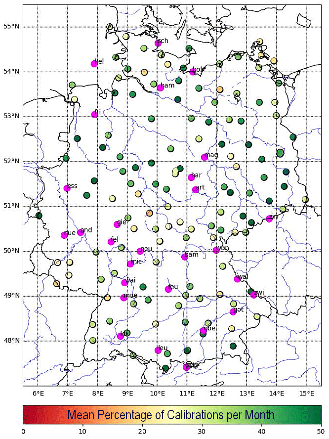
Figure 1 Lufft-CHM15k ceilometer network of the Deutscher Wetterdienst (DWD) in 2020, color coded by the number of available calibrations per month. Pink dots denote stations without calibrated data. Near-real-time QuickLooks and metadata information are available via http://www.dwd.de/ceilomap/ (last access: 25 March 2021).

2.3 Comparison of mixing layer height

The evaluated model MLH stems from the ECMWF IFS operational forecast, archived at steps $\mathrm{3},\mathrm{6},\mathrm{9},\mathrm{\dots },\mathrm{24}$ h based on daily 00:00 UTC analysis. The model determines the MLH at the critical value of the bulk Richardson number (Ri=0.25), which characterizes the degree of turbulence (Richardson et al., 2013). The vertical stability is estimated using the difference between each level and the lowest level. Several issues with this approach are described by, e.g., Engeln and Teixeira (2013), related to the Richardson number being based on ratios of both dynamic and thermodynamic vertical gradients rather than those of temperature and/or humidity as such, the use of dry variables in cloudy situations, and the fact that the Richardson number as a measure of local turbulence is often unable to properly characterize the turbulent properties of convective boundary layers. Turbulent kinetic energy, which could be used better, however, is rarely used in global models and as such is not available (Engeln and Teixeira, 2013).

The reference MLH observations are based on two approaches: visual inspection of daily 2-D time–height sections of β^∗(z) and the aerosol layer output from the CHM15k firmware. The former is quite reliable but elaborate and requires an experienced analysis of 2-D backscatter sections. The latter is automated and unbiased but suffers from severe inaccuracies and ambiguities and is mostly unrealistic in cases with multiple layers, low clouds/fog, small aerosol gradients, precipitation and long-range transport of dust, smoke, etc. In principle, MLH detection is a pattern recognition problem assuming that the vertical distribution of aerosol can be used as a tracer for boundaries. This, however, is not always the case. The absolute value of the backscatter is typically not needed since the relevant information seems to be coded in the gradient (but possibly of different orders) of the backscatter profile (Teschke and Pönitz, 2010) and its temporal development. The CHM15k firmware calculates up to three layers with quality flags from the range-corrected signal (P(z)z²) by means of a wavelet transform algorithm (Teschke and Pönitz, 2010). Which of these corresponds to the MLH, however, remains a decision according to specificity, temporal continuity and distinctness. In this respect, Haeffelin et al. (2012) find in their analysis of limitations and capabilities of existing mixing height retrieval techniques “… no evidence that the first derivative, wavelet transform, and two-dimensional derivative techniques result in different skills to detect one or multiple significant aerosol gradients”. While MLH reported by CHM15k definitely lacks reliability even when robust metrics like maximum daily mixing layer heights (MMLHs) are chosen, visual inspection of individual cases illustrates why algorithms fail with ubiquitous complex scenes and simultaneously provides reasonable estimates of MMLH. The uncertainty of visually inferred MLH is about ±100 m, and no MLH < 400 m a.g.l. can be detected due to artifacts from the overlap correction. Given all these limitations, the discussion of MLH is included in this article as it is the most prominent feature in the vertical profile, but it is not intended as a rigorous evaluation.

2.4 In situ measurements of particle composition and sizes

To interpret the model–observation differences, in situ particle composition measurements are used from the German GAW global station Hohenpeißenberg (HPB) (47.8^∘ N, 11.0^∘ E; 990 m a.s.l.), (Flentje et al., 2015). The Hohenpeißenberg station is located on a pre-Alpine hill, sticking out 300 m above the surrounding forest and/or grassland and represents rural central European conditions. Particle composition observations stem from the quadrupole aerosol chemical speciation monitor (Q-ACSM; Aerodyne Res. Inc., Billerica, MA, USA; Ng et al., 2011) and quartz-/teflon-filter probes analyzed for water-soluble ions with a DIONEX ICS 1000 (Henning et al., 2002) as detailed in Flentje et al. (2015). Both measurements' uncertainties are negligible for global model evaluation. Only the model vertical level of correspondence is not unambiguous to determine for mountain stations sticking out from the model orography. The profile evaluation circumvents this by excluding stations in steep terrain and through the negligible effect of the orography at higher altitudes. As a compromise for HPB (z_obs=995 m a.s.l., z_geopot-model=665 m) to capture both surface effects and ambient conditions at an elevated sampling level, we choose L54–L60 and L127–L137 for the 60L and the 137L model versions, respectively; see, e.g., Wagner et al. (2015). The range of concentrations within these altitudes indicates the uncertainty.

2.5 Concept of evaluation

Given the complexity of spatiotemporal variations of 14 interacting aerosol types in the IFS-AER model, it is important to reduce the evaluation to a meaningful subset of metrics and scores and adapt it to the information content of the observation data. This study focuses on the vertical aerosol distribution and the altitude dependence of the model–observation differences (bias) from about 0.3 to 6 km above ground. Below 0.3 km, the incomplete overlap cannot be corrected with sufficient accuracy. Above 6 km, ceilometer data suffer increasingly from low SNR and cloud artifacts. To avoid perturbation of our results by truncated profiles extending vertically over less than 0.6 km or containing clouds and possibly falling precipitation streaks, such profiles are excluded (see Sect. 4.2). In the vertical, we distinguish between the surface layer (SL) where the sources of most particles are, the ML and the free troposphere (FT), where long-range transport takes place. Model biases may indicate specific deficiencies in the model but may also stem from uncertainties in the observation data or the forward operator or arise from necessary adaptions of the data sets (see Sect. 4.2).

While there are several options to discuss the agreement of forecast and observed backscatter profiles, we use the following metrics and scores: the correlation of model–observation profiles evaluates their shape, i.e., efficiency and timeliness of vertical/horizontal transport, injection heights, representation of the mixing layer and stratification. This is jointly summarized in Taylor diagrams (Taylor, 2001) with the standard deviation coding the variance or amplitude of the profiles. The bias (as Mm⁻¹ sr⁻¹) or modified normalized mean bias (MNMB) (as a percentage) as a function of time and altitude evaluates the sources or sinks (strength) and physical and chemical transformations, separately for ASM and CTR:

$${\text{MNMB}}_{\text{asm, ctr}}(z,t)=\mathrm{100}\cdot {\displaystyle \frac{\mathrm{2}}{N}}\cdot \sum _{i=\mathrm{0}}^N{\displaystyle \frac{M_{\text{asm, ctr}}(z,t_i)-O(z,t_i)}{M_{\text{asm, ctr}}(z,t_i)+O(z,t_i)}},$$

where M_{asm, ctr}(z,t_i) and O(z,t_i) denote modeled and observed values at altitude z and time t_i, respectively. Either moving averages over selected altitude ranges (bias time series) or (e.g., monthly) averages resampled at the model levels (bias profiles) are calculated.

The MNMB is used for comparability within CAMS, because it is better suited to verify aerosol and chemical species concentrations compared to verifying standard meteorological fields. Spatial or temporal variations can be much greater, and the model biases are frequently much larger in magnitude. Most importantly, typical concentrations vary quite widely between different aerosol types, regions and heights, and a given bias or error value can have a quite different significance. It is useful therefore to consider bias and error metrics that are normalized with respect to observed concentrations and hence can provide a consistent scale regardless of pollutant type, altitude or region (see, e.g., Elguindi et al., 2010, or Savage et al., 2013). Moreover, the MNMB is robust to outliers and converges to the normal bias for biases approaching zero, while taking into account larger uncertainties in the observations and the representativeness issue when comparing coarse-resolved global models versus site-specific station observations.

Taylor polar plots combine two statistical measures for pairs of profiles, averaged over any optional period of time (here daily means or medians) and over different stations: the correlation of coincident pairs of modeled and observed vertical profiles plotted along the azimuth, and the standard deviation of model profiles normalized to the observation on the x axis (Taylor, 2001). This means that correlation is calculated over altitude ranges rather than periods of time. The ideal agreement or the reference point (observation) is thus located at the polar coordinate [1,1]. It is worth noting that the distance from the reference in Taylor polar plots corresponds to the root-mean-square error (RMSE); thus, Taylor plots powerfully display performance changes between model versions in a strongly aggregated way.

By considering mean and median values, the skills with and without (peaks of) events are distinguished, the latter representing more background conditions and less the interannual variability of (mostly dust) events. Negative and positive biases are denoted as “low bias” or “high bias”, respectively; their absolute amount is classified as large or small. The relative data coverage of 3-hourly profiles from all stations remaining for evaluation is 93 %, 92 %, 89 %, 83 %, 71 %, 46 % and 16 % at 0.4, 1, 2, 3, 4, 5 and 6 km above ground, respectively.

3 Results

3.1 Bias and MNMB

Figure 2 shows the temporal evolution of bias (upper panels) and MNMB (lower panels), each for ASM (red/orange) and corresponding CTR (green/blue) around vertical model levels spaced by 1 km ($\mathrm{0.4},\mathrm{1},\mathrm{2},\mathrm{\dots }\mathrm{6}$ km above ground), each averaged over ±one model level. The data averaged over 21 German ceilometer stations become statistically sparse at higher levels (≥ 6 km). A different perspective, transformed to the whole vertical profiles of monthly mean and median bias of β^∗(z), is shown in Fig. 3 and color coded by each month for 2016 to 2019. Actual β^∗(z) profiles are shown for comparison in Figs. D1 to D4. The following results refer to Figs. 2 and 3.

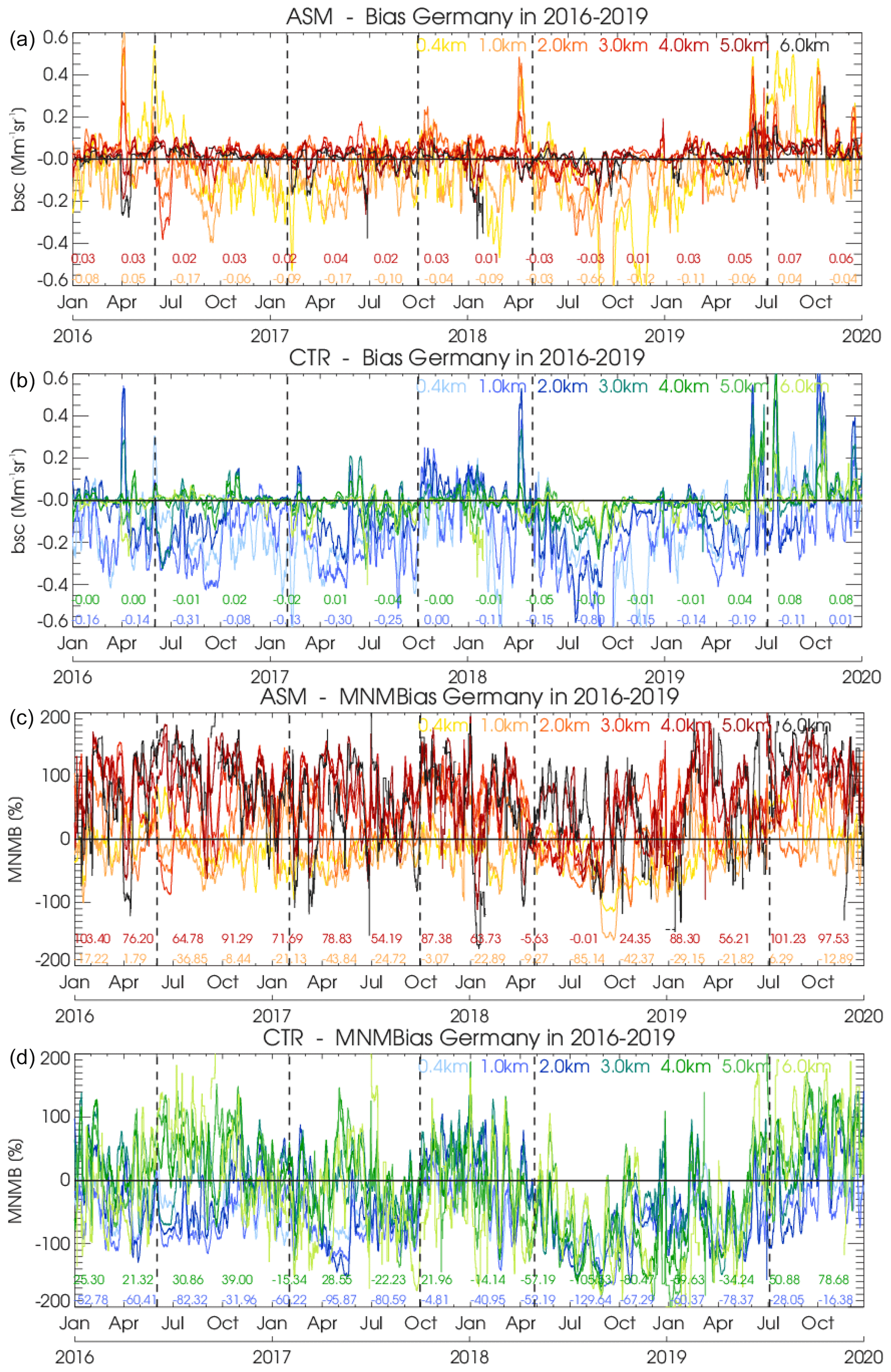
Figure 2 The 7 d running mean bias of β^∗(z) from ASM (a) and CTR (b) combined from 21 German stations in 2016–2019. Same for MNMB in panels (c) and (d). Colors refer to different altitudes above ground. Vertical black lines indicate major model updates as in Table 1.

The bias of β^∗(z) shows a clearly different behavior near the surface, in the ML and the FT, with upward tendencies toward the surface, low bulges in the ML, reaching up to ≈ 0.5–1 km in winter and ≈ 1–2 km in summer, and enhanced variation related to irregular long-range transport, mostly of dust, in the FT as shown in Fig. 3. Estimated error bars overlaying the CTR profiles indicate the significance of the biases. The low-bias dips above 6 km are artifacts caused by cloud boundaries not captured by the quality control. Due to events, the mean bias is on average larger and scatters more than the median, particularly in the FT, which holds little aerosol in undisturbed situations. Throughout several months, Saharan dust events cause a large high bias in the upper ML and the FT. A positive impact of the assimilation is reflected by a smaller and less variable bias in ASM than in CTR, as shown in Fig. 2, where 7 d running means remove the tremendous variability on daily timescales. Bias and MNMB tend to be lower in CTR (blueish) than in ASM (reddish), particularly at lower heights. ASM bias/MNMB show less longer-term variation with model changes and seasons and less vertical spread. (Note that only ASM is used with cycle 41r1 before June 2016.) MNMB is less sensitive to absolute β^∗(z) and thus more clearly shows phases of vertical association and dissociation, and an overall downward trend in 2016–2018 of CTR MNMB turning into an increase in 2019. For ASM, this variation is only evident in the FT. With cycle 46r1, bias and MNMB in ASM and CTR are vertically closer associated.

Over the 4 years, monthly bias profiles have become more variable, the means more than medians and CTR more than ASM (Fig. 3). This may reflect changes to model source strengths (see Table 1), larger errors during more frequent events and a balancing impact of the assimilation, respectively. This scatter is particularly observed in the ML where model β^∗(z) values are on average lower than observed until July 2019 and higher thereafter. Particularly CTR shows lower β^∗(z) bias and MNMB around summers at low heights (MNMB around −100 %), while ASM remains flatter thanks to the assimilation (Fig. 2). SL biases stick out high (up to 0.3 Mm⁻¹ sr⁻¹) with cycle 41r1 T255 in spring 2016 and with cycle 46r1 after July 2019 (up to 0.4 Mm⁻¹ sr⁻¹). In between, they were smaller or negative as shown in Fig. 2 and Table 2. A bias increase with cycle 46r1 at 0.4/1 km a.g. corresponds to overestimated NO₃, NH₄ and OM in the model, as discussed with respect to GAW surface data in Sect. 3.3.

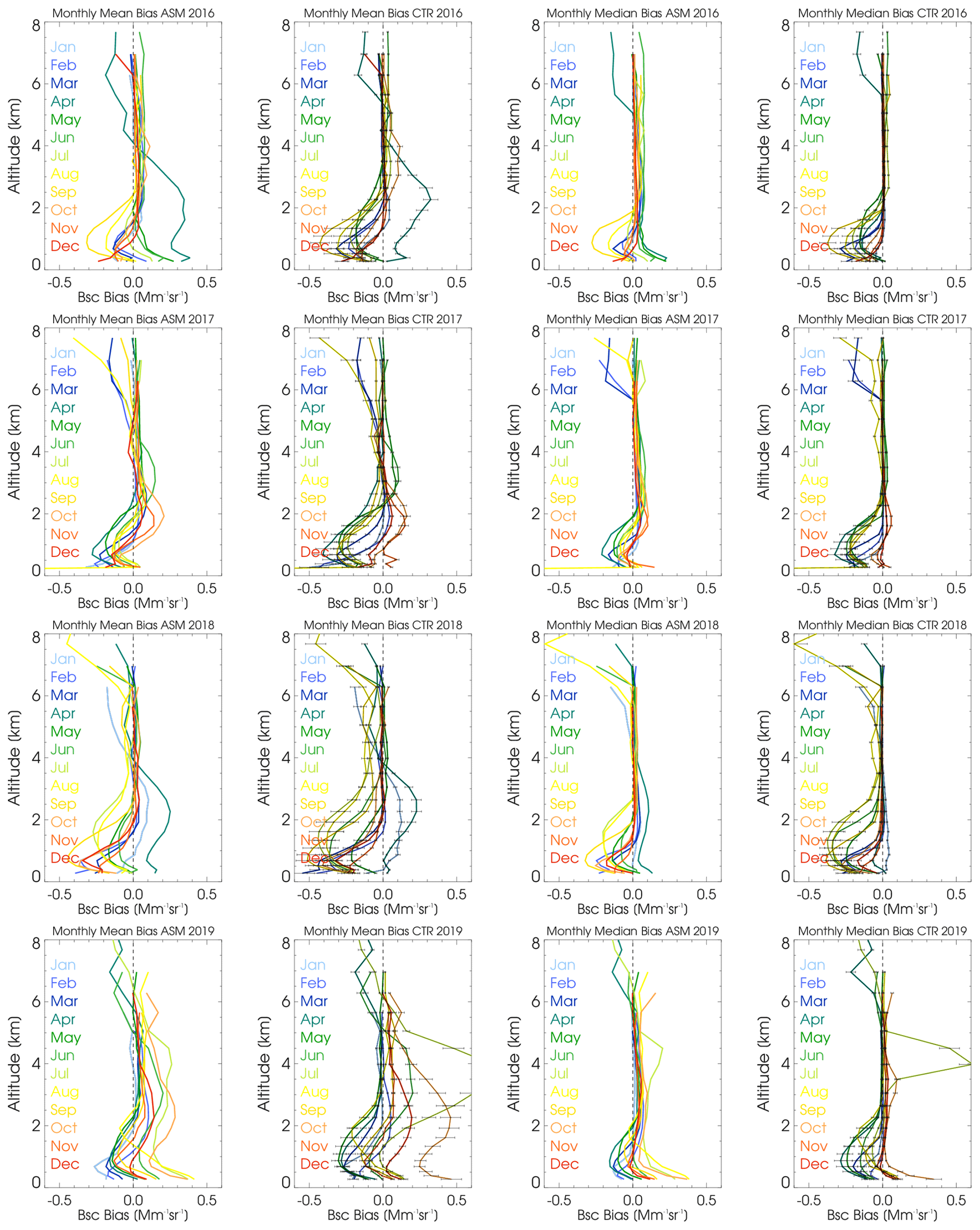
Figure 3 Monthly mean (left pair) and median (right pair) profiles of bias ASM/ceilometer (left) and CTR/ceilometer (right), combined from 21 German stations in 2016–2019. At higher altitudes, the profiles are partly contaminated by remaining cloud artifacts.

Though seasonal regularities are disturbed by five irregular model updates in the 2016–2019 period, bias/MNMB in ASM show opposing seasonal cycles in the lower (0.4 km a.g.) and the upper (2 km a.g.) ML with amplitudes of 0.2 Mm⁻¹ sr${}^{-\mathrm{1}}/\mathrm{40}$ % (summer maximum) and 0.1 Mm⁻¹ sr${}^{-\mathrm{1}}/\mathrm{70}$ % (summer minimum), respectively (Fig. 4). Figure 2 shows this particularly before cycle 43r3 in October 2017. The seasonal amplitude is small at the intermediate level 1 km a.g. The summer minimum is evident up to 3 km (MNMB even to 4 km a.g.), while it is variable due to Saharan dust events at 5 and 6 km a.g. A weekly cycle is not significant in the bias nor the MNMB, indicating a negligible influence of short-term anthropogenic emissions which are not captured by the inventories' temporal resolution (1 month).

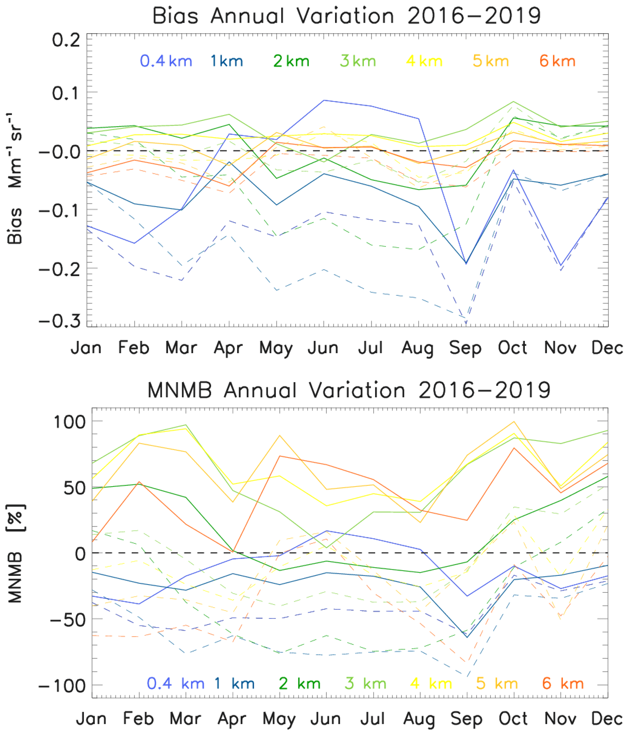
Figure 4 Annual variation of bias and MNMB of β^∗(z) for ASM and CTR (dashed) combined from 21 German stations in 2016–2019.

Periods with opposing high bias in SL or ML and low bias in FT indicate vertical displacement of aerosol within the profile. While expected within individual profiles, it often also lasts for longer periods, as shown in Fig. 2, e.g., in April–June 2016 and repeatedly until cycle 45r1 in mid-2018, whereupon it largely disappears. Longer periods are evident as oscillations even in the monthly mean profiles in Fig. 3. The effect is more distinct for ASM and may be attributed to adaptions by the assimilation of AOD which adds no direct height information. Spatiotemporal shifts between the model and observations result in low-bias or high-bias oscillations with time and mostly cancel out within a day. The corresponding fractional skill score is discussed in Sect. 3.4.2. Outstanding high-biased monthly profiles (Figs. 3 and 2) or high-bias peaks are mostly related to Saharan dust events, e.g., in April and June 2016, June, July and October 2017, January and April 2018 and June–July and October–December 2019 (see Sect. 3.4.1). However, occasionally, SD particles induce cloud formation (e.g., 16–17 October 2017) which largely increases the β^∗(z) signal in spite of the constant dust aerosol load (see Appendix B). Until this exceeds the β^∗(z) threshold above which ceilometer data are removed as clouds, such events produce a low bias. Low biases also occur in the ML (1–2 km lines in Fig. 2) during smog periods, e.g., when transport of highly polluted air from eastern Europe towards Germany (January 2017, February/March 2018) is not captured by the model (low bias of −0.3 Mm⁻¹ sr⁻¹ in February–March 2018; cf. Sect. 3.3). At higher altitudes ≥ 5 km, remaining cloud artifacts within sparse data coverage (low SNR) cause sharp low-bias dips in Fig. 2.

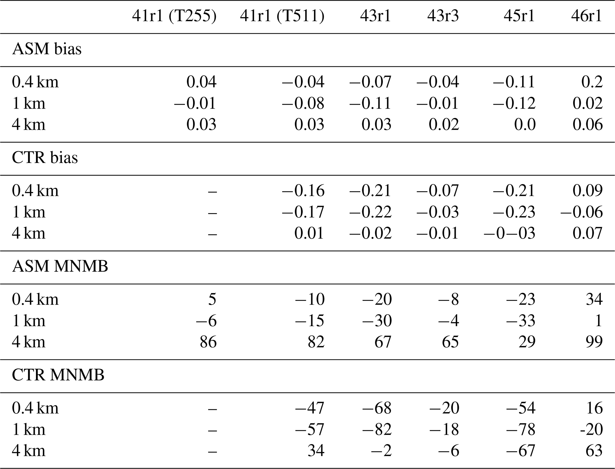
Table 2 Bias [Mm⁻¹ sr⁻¹] and MNMB [%] of β^∗(z) for ASM and CTR runs at 0.4, 1 and 4 km altitude above-ground averages within the different model configurations of Table 1.

3.2 Profile shape – correlation

The Pearson correlation coefficient (r) of model–observation β^∗(z) profile pairs specifically quantifies the covariance of vertical variability, i.e., the shape of the profiles, independent of the bias. The ML and eventual particle plumes in the FT govern this correlation. Again, elimination of clouds and the overlap range is essential. Apart from large event-driven situational variability, the profile correlation exhibits no long-term tendency but displays a clear seasonal cycle with better agreement in winter and less in summer, as shown in Fig. 5. Overlain in Fig. 5 are vertical lines indicating seasonally irregular model upgrades and mean values over the IFS cycle periods from Table 1. The mean correlations within the IFS configuration periods do not vary significantly (cf. Table 2), and their differences reflect the seasonal cycle rather than indicating changes of the model performance. Individual (3-hourly) profile pairs or longer temporal averages have been considered, whereby the former penalizes already small time shifts or displacements (and yields lower r). Diurnal or longer averages reduce influence from early/lagged transport as well as the dominant diurnal cycle of the ML and are more sensitive to irregular events. On a monthly basis, also median profiles are considered to evaluate specifically the model background profile (Appendix D, Figs. D1–D4).

Figure 5 Pearson's correlation coefficients (r; a), standard deviation normalized towards ceilometer observations (b) and integrated bias of daily average β^∗(z) profiles of IFS-AER versus ceilometers for 2016–2019. Red crosses denote ASM; blue crosses denote the control run. The 3 d moving average line and median values over the periods with constant model configurations are added.

Generally, increasing correlation is found between IFS-AER fields and individual station profiles, with longer averaging times: while only 50 %–60 % of the observed 3-hourly vertical variability is explained by IFS-AER (r_3hly=0.5–0.6), the explained fraction increases to 70 %–80 % for diurnal average profiles (r_1dly=0.7–0.8) as shown in Fig. 5. Thus, spatiotemporal aggregation defines the information to be revealed. Aerosol changes are very often not timely and/or (vertically) displaced on a timescale of a few hours, but longer (or more extended) events and developments are quite reliably captured by IFS-AER. This is particularly true for Saharan dust transport where nearly all events are reproduced but the large concentrations (large β^∗(z)) combined with small-scale inhomogeneity give rise to larger uncertainties as well (see Sect. 3.4.1). The middle panel of Fig. 5 shows the variance and provides numbers of daily average vertical profiles normalized to that of the observations as normalized standard deviation (NSD). The time series and Table 3 reveals marked differences between the IFS cycles, given for ASM/CTR, separately: profile variance approaches the observations (NSD $=\mathrm{0.97}/\mathrm{0.93}$) during cycle 41r1 before June 2016 and NSD $=\mathrm{0.95}/\mathrm{0.96}$ during cycle 46r1. Only about half the observed variance is simulated during cycles 41r1 after July 2016 (NSD $=\mathrm{0.52}/\mathrm{0.50}$), 43r1 (NSD $=\mathrm{0.46}/\mathrm{0.45}$) and 45r1 (NSD $=\mathrm{0.51}/\mathrm{0.52}$). Intermediate values (NSD $=\mathrm{0.67}/\mathrm{0.78}$) are found during cycle 43r3. A similar measure like NSD (analog to AOD bias) is the vertically integrated β^∗(z) bias. It is dominated by the ML and/or events as in Fig. 2 but has the limitation that every single profile has weather-dependent vertical extension. No clear ruptures as for NSD appear at the model upgrade times for the integrated β^∗(z) diurnal profile bias in Fig. 5c. It is not clear whether this can be interpreted in terms of model upgrades where several adaptions of sources took place. For example, sea salt as a large contributor to high β^∗(z) bias in the ML (Chan et al., 2018) was reduced inland after June 2018 by redistributing mass from fine to coarse particles (Rémy et al., 2019). As of July 2019, NO₃ and NH₄ were added and probably too much, as discussed in Sect. 3.3. On the other hand, the substantial increase of the OM load in February 2017, clearly evident at the surface (Sect. 3.3) seemingly did not affect the profile integral.

A more condensed way than Fig. 5 to descriptively visualize performance changes between model versions is Taylor polar plots, as displayed in Fig. 6 and explained in Sect. 2.5. Here, the average performance during the six IFS-AER configurations in Table 1 are summarized in terms of correlation, normalized standard deviation and the plotting distance towards the reference, i.e., the root mean square error (Taylor, 2001). Accordingly, the model system has not systematically evolved towards improved representation of the profile shape, though mean values around r_1dly=0.7 are already quite good. However, after some changes, finally the overall variance of the profile became nearly realistic on average after the implementation of NO₃ and NH₄ and adaptions to SO₄, organics and dust in cycle 46r1 in July 2019. The differences between ASM and CTR are small. It should be noted that individual covariances of modeled and observed profiles vary quite strongly with time and location/station, meaning that many situations cannot be closely captured and even the observations may partly not be representative due to undetected artifacts (clouds, overlap correction, misalignment, etc., not removed by the quality control).

Figure 6 Taylor plot combining Pearson's correlation coefficients (azimuth) and standard deviation normalized towards ceilometer observations (radius) from daily average β^∗(z) profiles of IFS-AER versus ceilometers for 2016–2019. (a) Median of all data; (b) mean over 221 Saharan dust days as defined in Sect. 3.4.1. Red dots denote ASM; blue dots denote the corresponding CTR. Note the different x and y axes.

3.3 Particle composition and size at surface level

To better understand the differences between modeled and observed backscatter β^∗(z) profiles, near-surface mass concentrations MC of the prognostic aerosols in IFS-AER, namely PM₁₀, sulfate (SO₄), nitrate (NO₃), ammonium (NH₄), BC and OM as well as qualitative proxies for sea salt (SS) and mineral dust (MD) are compared to surface in situ observations. All particle concentrations are modeled and measured (in situ) in dry state without hygroscopic water uptake. PM₁₀ is calculated from the model mass mixing ratio (mmr) according to the formula used in IFS-AER (Rémy et al., 2019): PM₁₀ = ρ([SS${}_{\mathrm{1}}]/\mathrm{4.3}+[$SS${}_{\mathrm{2}}]/\mathrm{4.3}+[$MD₁]+[MD₂]+0.4[MD₃]+[OM]+[BC]+[SO₄]+[NO3₁]+[NO3₂]+[NH₄]), whereby [X_i] denotes the mmr of the ith size bin of the size-resolved species and ρ is the density of air. The “dust” variable is not directly measured but approximated by MD = PM₁₀−[OM]−[BC]−[NO₃]−[NH₄]−[SO₄]−[Cl] and inferred on event basis to discuss contingency of events in Sect. 3.4.1. Mineral dust sizes at HPB are mostly smaller than 10 µm and its composition is largely disjunct from the other IFS-AER particle types. Chlorine (Cl) is used as a proxy for NaCl in sea salt, stoichiometrically corrected for the sodium Na portion ($m_{\mathrm{Na}}/m_{\mathrm{Cl}}\approx \mathrm{22}/\mathrm{35}$) and for ≈ 7 % of additional minor components like SO₄, Mg, Ca, etc. A rigorous evaluation of composition-resolved MC is beyond the scope of this article, but a sanity check with data from the GAW global station (HPB) provides insight into the representation of individual aerosol types.

Table 3 Concentrations [µg/m³] of IFS-AER prognostic aerosols by ASM and CTR versus GAW in situ measurements at the Hohenpeißenberg station, averaged over constant model configuration periods as defined in Table 1.

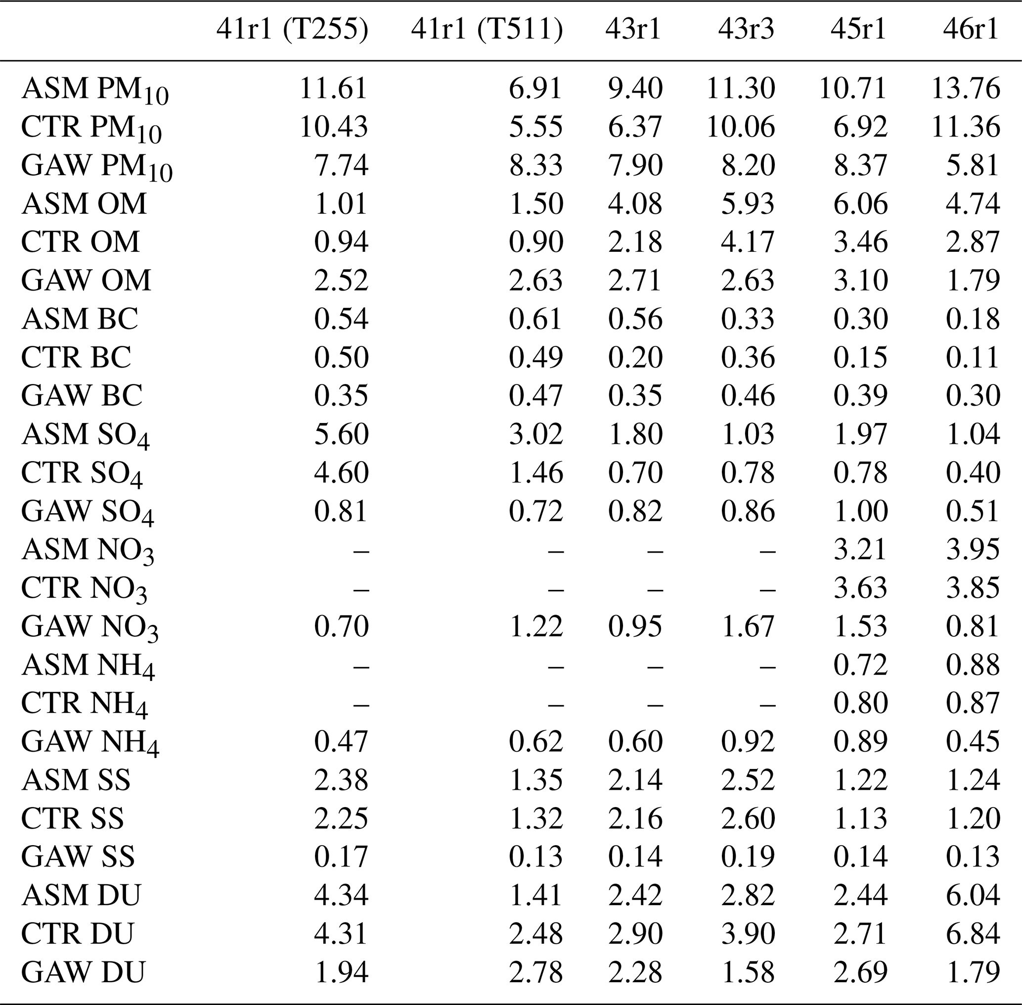
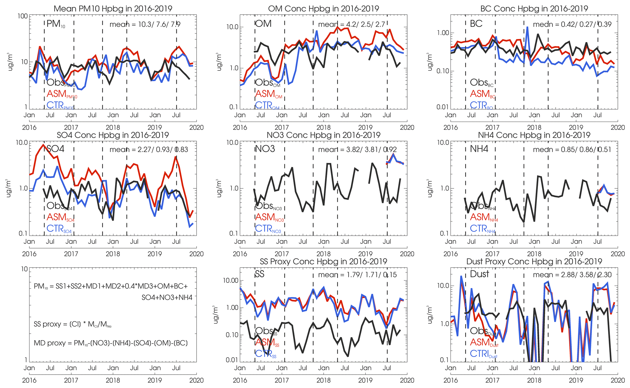
Figure 7 Comparison of mass concentrations averaged over IFS levels L54–L60/L127–L137 for L60/L137 model versions and measured by ACSM and filter probes at the Hohenpeißenberg GAW station for 2016–2019. From the top left to the bottom right: PM₁₀, OM, BC, SO₄, NO₃ and NH₄, chlorine, sea-salt and dust proxies as described in the text. Vertical black lines indicate major model updates as in Table 1. Note the different y ranges!

As shown in Fig. 7, the dry surface mass concentration PM₁₀ for ASM (10.3 µg/m³) and CTR (7.9 µg/m³) roughly corresponds to HPB data (7.9 µg/m³). The assimilation seems to bias surface concentrations a bit high. Species are detailed in Table 3. PM₁₀ approaches HPB data after the increase of OM with cycle 43r1 (February 2017), though this was partly compensated by a parallel decrease of SO₄; it is, however, overestimated as of cycle 46r1 after July 2019 due to the introduction of NO₃ and NH₄, which are simulated roughly 3 µg/m³ (∼300 %) and 0.3 µg/m³ (∼60 %) too high at HPB, respectively. Further changes with cycle 43r3 (October 2017) synchronize the phase but exaggerate the amplitude of the SO₄ annual cycle which together with the dominating high-biased contribution from OM causes most of the PM₁₀ overestimation near the surface in summers since 2018. After sulfate was reduced in cycle 43r3 and beyond (Rémy et al., 2019), SO₄ in CTR agrees remarkably well with HPB, while summer concentrations are by 2–4 µg/m³ too high in ASM. BC, which contributes only about 5 % in mass, has evolved quite realistically with a slightly more decreasing trend in 2016–2019 than observed. Probably, emission inventories overestimate the decreasing trend over Europe where the decline has leveled off in the last decade.

Total suspended sea salt is equally overestimated in ASM and CTR with mean MC around 1.8 µg/m³, while the estimated abundance at the far inland HPB site is only 0.02–0.3 µg/m³, however with large error bars of ±0.3 µg/m³ due to the hard-to-sample coarse mode (5–20 µm) which contributes about 0.3 µg/m³ to the SS concentration in the model. The seasonal variation by roughly an order of magnitude seems realistic. The large uncertainties and increases of bias in the PBL associated with SS has already been discussed in Chan et al. (2018). To this end, the above-mentioned approximation of SS via Cl has a negligible impact. The observed dust proxy contributes only 4 %–6 % to the annual average mass at HPB (Flentje et al., 2015). The seasonality is reproduced, but mean summer contributions around 10 µg/m³ would require much more events than observed and simulated, which confirms that dust concentrations are overestimated not only near the surface but also in the higher ML and the FT, as noted in Sect. 3.1. The assimilation correction to dust MC of few µg/m³ is too small. These results are not affected by mass-to-backscatter conversion nor humidity and, due to averaging over the lowest 300 m a.g., are not sensitive to the model level selected to represent surface concentrations at HPB. The regional representativeness is limited to rural central Europe (Putaud et al., 2010) where comparatively small concentrations prevail, as discussed in Sect. 4.

3.4 Long-range transport

The DWD ceilometer network follows the 3-D dispersion of optically efficient particles like dust or smoke and is therefore particularly suitable to verify the timeliness of long-range aerosol transport in IFS-AER in a qualitative way. Against this, automated rendering of 2-D time–height sections from the ensemble of stations to evolving 3-D fields is a challenge beyond the scope of this article, and advanced metrics like fractions skill score (Roberts, 2008) still have to be adapted. Simpler options are to compare time–height slices at fixed locations (stations), analyze representative cases or evaluate the representation of events qualitatively. In aged air masses far from the sources, chemical transformations slow down and transport of particle layers/plumes becomes more passive. This reflects in wide consistency of aerosol fields in the IFS model with large-scale dynamical structures in the middle and upper troposphere (e.g., Flentje et al., 2005).

3.4.1 Mineral dust

The previous sections showed that Saharan dust loads over Germany are overestimated at the surface and throughout the profile. The realistic seasonality (Fig. 7) and the reasonable correlation (Fig. 5) however suggest that time and also vertical position of SD plumes are mostly captured in IFS-AER, as long as the scales are sufficiently large. It can further be shown that IFS-AER forecasts have a high score in capturing or reliably excluding significant Saharan dust days (SDDs), which are inferred from the observations by visual inspection of 2-D network composite plots and backward trajectories and from the model by choosing a reasonable threshold for maximum dust AOD within a box of 1^∘ × 1^∘ around selected ceilometer stations. Defining days with maximum AOD_{550 nm,dust}>0.03 (maximum AOD_{550 nm,dust}<0.001) as SDDs (non-SDDs) in the model and within the inherent uncertainties of type identification, these threshold yield “excess” and “miss” rates near zero, 221 “hit” days and 271 zeroes. Hits (zeroes) are SDDs (clear days) identified in both data sets; “excess” SDDs are simulated but not observed and “misses” denote observed SDDs that are not reproduced by IFS-AER. Due to the uncertain identification of faint aerosol layers based on ceilometers and trajectories, the majority (two-thirds) of days in between these thresholds remain unclassified. This is, however, no severe limitation to this analysis, which is meant to confirm qualitatively the high reliability of the forecasts with respect to decided SDDs and non-SDDs.

As several improvements were made to emission, size distribution and (wet) deposition of dust (Rémy et al., 2019), a Taylor diagram for the subset of SDDs with modeled maximum AOD_{550 nm,dust}>0.03 in Fig. 6 shows the development of dust simulation by IFS-AER during the 2016–2019 period. On SDDs, the correlation of profiles (shapes) is lower (r=0.4–0.6 instead of r=0.6–0.8), while standard deviation (coding the amplitude of β^∗(z)) is higher. The first indicates spatiotemporal or vertical shifts of layers/plumes, the latter reflects overestimation of dust concentrations but is not directly scaled to the SD bias due to the large influence of the ML on the profile. These findings confirm the analysis by Rémy et al. (2019) who state a good capability to reproduce dust events as detected by Aerosol Robotic Network (AERONET) station data (Holben et al., 2001). According to the different trajectories, the long-range transport pathway (via the Atlantic, Mediterranean, etc.) does not effect the accuracy of timing/positioning of plumes, while the scale reduction during regional stirring and dispersion is the main reason degrading the representation of the vertical profile shape.

3.4.2 Fractions skill score

The penalizing of slightly vertically displaced aerosol layers yielding a low or even anti-correlation in Sect. 3.2 hints to the fact that a useful assessment of the positioning (in space and time) of an aerosol plume requires not only a reference to point locations but also to their vicinity. Such a skill score shall distinguish nearly correct positioned features from deviations by a bigger margin. An approach to quantify the degree of overlap of simulated and observed aerosol structures is the fractions skill score (FSS; Roberts, 2008; Skok and Roberts, 2016). The perceived accuracy increases with larger scales, longer averaging, elimination of outliers, etc. Thus, reasonable scales must be analyzed to balance the processes of interest and the useful level of detail to be notified. For example, small (subgrid)-scale structures appear randomly displaced or missed because the information content of the model fields does not match the resolution of the observations, which the other way round, are not representative for the model grid box. For profile correlation, the usefulness threshold of scales is for IFS-AER presently of the order of 0.5 d and 100 km. An approach towards FSS would be to draw polygons either outlining the boundary of an individual SD plume observed at a given time at different ceilometer stations or, alternatively, refer to the overlap of plumes in time–height sections at individual stations. Another metric to quantify the model performance for coherent plumes in a quasi-stationary flow is the relative deviation of arrival/departure times of plumes/layers at station positions in model and observation as visualized in Fig. 8 for the SD plume on 16 October 2017. Composite bullets with color-coded arrival times observed in 2-D β^∗(z) ceilometer sections (outer ring) and corresponding model fields (inner bullet) illustrate the slightly delayed arrival (0–1 h) of the model plume in western Germany, its catchup in the middle and again lagged arrival (0–2 h) in the eastern part. The uncertainty of determination is about 1 h. This plume was neither observed nor simulated in the very south of Germany.

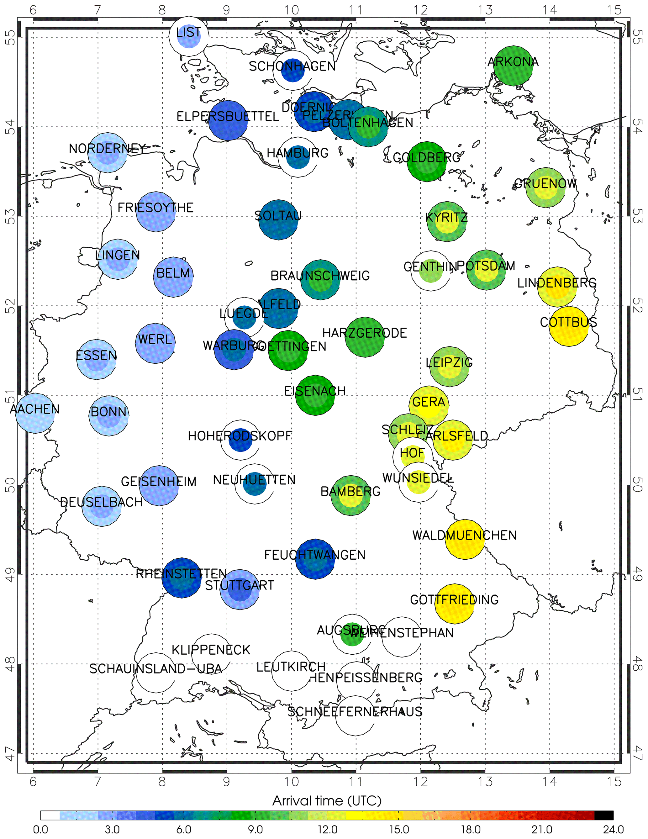
Figure 8 Arrival time of individual SD plume on 16 October 2017, color coded by the hour of day, as measured by ceilometer (outer ring) and IFS-AER (inner bullet). Missing data are in white: the selected plume did not reach the southernmost part of Germany or arrival could not be identified due to low clouds.

4 Discussion and conclusions

Thorough evaluations of IFS-AER operational forecasts are regularly published in near-real time or in retrospective validation reports on the CAMS website (http://macc-raq-op.meteo.fr/, https://atmosphere.copernicus.eu/eqa-reports-global-services/, last access: January 2021), as presented by Eskes et al. (2015). In these, the realism of the vertical profile has not yet received much attention, although it may be relevant for aircraft guidance around volcanic ash layers, in cases of visibility reduction during Saharan dust events, for the cloud formation potential, weather and radiation transfer or the dispersion of severe pollution events. Our focus on the vertical aerosol distribution complements evaluations based on AOD columns (Rémy et al., 2019; Gueymard and Yang, 2020) and surface in situ measurements (e.g., https://atmosphere.copernicus.eu/index.php/regional-services/, last access: January 2021). It extends our study by Chan et al. (2018) (CH18) from the surface layer up to the mid-troposphere. Yet, our results are shown to be consistent with previous verifications. The vertical profile of β^∗(z) bias allows a more detailed understanding of the height dependence of sources and sinks, vertical transport and redistribution of particles as well as temporal shifts in the model as FT biases are governed by long-range transport rather than by surface drag and convection in the mixing layer. Verifications of IFS-AER reanalyses reported by Flemming et al. (2017), Inness et al. (2019) and Wagner et al. (2021) are in many respects representative for the operational forecasts.

Compared to our first study by CH18, covering the period September 2015–August 2016, we use the 4-year period of 2016–2019 with an overlap of 8 months, and we use data from 21 instead of 12 ceilometer stations and all evaluable altitudes. As no clear dependence of performance on the distance to model grid points was found in CH18, and the spatial resolution was increased from T255/L60 (≈1^∘ × 1^∘) to T511/L60 (≈0.5^∘ × 0.5^∘) during cycle 41r1 in July 2016, we drop the constraint to stations within 20 km around model grid points. Again β^∗(z) is used as this is the primary measured quantity of ceilometers that can be rigorously calculated from the IFS-AER output. The small high bias with large standard deviation of 1.5 times the model average found by CH18 for near-surface-integrated (0.2–1 km altitude) β^∗(z) is confirmed by our analysis at the lowest selected levels at 0.4 and 1 km a.g., as listed in Table 2. The larger overestimation of β^∗(z) associated with higher sea-salt-relative contributions is in CH18 partly (∼10 % of total β^∗(z)) attributed to the utilized hygroscopic growth scheme from the Optical Properties of Aerosols and Clouds (OPAC) database (Hess et al., 1998) and is not elaborated further in this study. Sea salt over continental Europe remains considerably overestimated (see Sect. 3.3) in all seasons as changes to the sea-salt emission scheme, e.g., coming in with cycle 45r1 (June 2018), still primarily aim to reduce the global low bias of sea-salt abundance dominated by oceans. Concurrent substantial increases of sea-salt particle sizes and sinks (wet deposition) likely reduce sea-salt mass concentrations further inland, apparent as steps at HPB in Fig. 7 but are either not efficient enough or still not the governing processes. As in Chan et al. (2018), underestimated near-surface β^∗(z) values are partly linked to unresolved local or regional scale (e.g., January–February 2017) emission events that reach up to 2–3 km a.g. (Fig. 2). Being stronger and more frequent in winter (Fig. 4), they contain much ammonium and nitrate (as NH₄NO₃) in the ML, which had not been included in the model by that time (Sect. 3.3). Increase of OM emissions in February 2017 (≈ 30 %–60 % of aerosol mass in the rural central European ML) and addition of nitrate and ammonium in July 2019 (≈ 10 %–30 % of aerosol mass as NH₄NO₃ or NH₄(SO₄)₂) clearly tuned the model towards observed concentrations/β^∗(z) and notably reduced the correction by the assimilation (Figs. 2 and 5). Similarly low MNMB in PM₁₀ was found for this event by Rémy et al. (2019).

Vertically displaced aerosol layers (often SD) causing low-bias or high-bias oscillations (Figs. 3 and 2) cancel out in vertically integrated backscatter (Fig. 5) and AOD (not shown) but degrade the profile correlation and are mostly not reduced by the assimilation. As described by Benedetti et al. (2009), the IFS-AER 4D-Var assimilation scheme based on AOD columns could add vertical aerosol information by adaptions to the vertical temperature, humidity or wind profiles, but the effect, e.g., by optimizing wind shears, seems not specific enough to improve the simulated aerosol profile in ASM relative to CTR. Generally, performance changes of IFS-AER with height are linked to specific processes.

Surface layer. Regional sources typically have the largest effect to the lowest part of the profile. In the near-surface layer, the observed high bias of NO₃ mass concentrations results from too efficient gas-to-particle partitioning, i.e., fine-mode NO₃ production from HNO₃ neutralization by NH₃, followed by temperature-dependent dissociation to NO₃ and NH₄. Secondly, remaining HNO₃ may heterogeneously produce coarse NO₃ on SS or dust particles (Rémy et al., 2019), but this process is of minor relevance in central Europe where fine-mode nitrate has a roughly 5 times larger mass concentration than coarse-mode nitrate. NH₄ is simulated at comparable concentrations as observed at HPB, while NO₃ is about 4 times as high. For fine-mode NO₃, the most efficient sink near the surface, probably underestimated, is dry deposition (Zhang et al., 2012), while sedimentation of small particles should be slow and is disabled in the model. Below-cloud wet deposition (washout) should affect the whole profile rather than only the surface where the high-bias tendency toward the ground is found (Sect. 3.2). The increase of resolution from 1 to 0.5^∘ in June 2016 excluded Munich from the HPB grid box, which may contribute to the marked decrease of PM₁₀ and SO₄ around this time as in Fig. 7. Since then, it should be representative of HPB including only small surrounding towns and rural area. A particular value of the assessment with respect to mass lies in its independence from hygroscopic growth with humidity and any mass-to-optical conversions, which have a particularly large impact on SO₄ and OM (Hong et al., 2014). The general bias increase towards the surface evident in Fig. 3 may be caused by too-slow vertical transport of surface emissions along with overestimated sources. SO₄ is overestimated in ASM in summer, while typical central European surface concentrations in winter are met (Fig. 7). Together with dust, this causes most of the bias' seasonal cycle in Fig. 4. The reason for the worsening mass input at surface level by the assimilation is not clear. OM has been a few µg/m³ too high during all seasons since February 2017. BC shows a step down with cycle 43r1 in February 2017 and (except January/February 2017) a further downward tendency until 2019 at realistic concentrations in ASM. Emission inventories thus seem to capture the decrease of anthropogenic emissions during the last decade, but as for SO₄ the assimilation seems to add too much mass and may disturb the realistic partitioning between anthropogenic and biogenic OM. Overall, average MNMB in the SL ranges from −23 %–34 % for ASM and from −68 %–16 % for CTR.

Mixing layer. Against overestimation of mass concentrations and β^∗(z) near the surface, the aerosol load in the ML tends to be biased low. Main reasons may be sources or delayed vertical transport from the surface. Further, the forward operator, including mass-to-volume conversion, presently uses particle densities of the pure materials, not taking into account possible porosity of dry atmospheric particles enclosing air due to coagulation and variable internal mixing (Winkler et al., 1981). If the model assumed larger bulk densities than particles actually have, the equivalent volumes were calculated too small and optical properties would be underestimated, because they depend strongly on the particle size. The density of accumulation-mode particles, composed of hydrophilic and hydrophobic materials could be overestimated by up to a factor of 1.5, which transfers to a factor of 1.3 in the optically relevant surface area. Secondly, the ML top is too smooth which means the capping transport barrier at the ML top seems less effective in the model, diluting higher ML concentrations with cleaner FT air. This aerosol mass would be missing in the ML, yielding a too-low amplitude (coded in the standard deviation) of the model compared to observations (reference) in the Taylor plots, too. Geometrically, however, the ML height on average seems reasonable (cf. Sect. 4.1). The monthly mean beta-star profiles suggest that aerosol mass, added to the column by the assimilation, results in overall higher aerosol load than in the control runs until July 2019, but the assimilation does not sharpen the transition from the PBL to lower values in the FT. Though it must be noted that averaging may considerably smooth the ML top by mere variation of PBL heights. Average MNMBs in the ML are mostly negative between 1 % to −33 % for ASM and −18 % to −82 % for CTR.

Free troposphere. The FT background might be biased slightly high due to the weak transport barrier, mass attribution by the assimilation or irregular transport of Saharan dust, which (as in CH18) is found to be overestimated over Germany by typically a factor of 2 or more all the time. CH18 calculated that accounting for non-spherical particles, using conversion coefficients based on T-matrix calculations rather than Mie theory, would reduce β^∗(z) by 15 %–45 %. This reduction arises from the modification of the phase function by non-sphericity, coded in the lidar ratio (LR), and not the specific extinction and thus does not transfer to AOD. In order to reduce the high dust bias in the model, the dust source size distribution after cycle 43r1 was modified to distribute less mass into the fine (8 % to 5 %) and more mass into the super-coarse bin (61 % to 83 %) which has a shorter lifetime due to faster sedimentation (Rémy et al., 2019). An according dust reduction, however, cannot be seen over Germany in the mass concentrations of the dust proxy in Fig. 7, which is independent from uncertainties in the mass-to-β^∗(z) conversion. Monthly median bias in the FT is mostly not significant and < 0.1 Mm⁻¹ sr⁻¹; average MNMB ranges from 29 %–99 % for ASM and from −67 %–63 % for CTR. That the observed inflation of the β^∗(z) signal on 17 October 2017 (Sect. B) marks the onset of water cloud formation, seems plausible. The temporary factor of 10 increase of β^∗(z) ($\sim \mathrm{1}\times {\mathrm{10}}^{-\mathrm{6}}\to \sim \mathrm{1.2}\times {\mathrm{10}}^{-\mathrm{5}}$; Fig. B2) roughly corresponds to a significant visual range reduction by an order of magnitude (to ∼ 1 km assuming a lidar ratio near 30 sr). On the other hand, a mature water cloud would block the lidar beam and any signal from above (Fig. B1, ∼ 04:00–07:00 UTC), which seems to be the case at some stations further north (not shown). Alternatively, the passage of a shallow plume with 10 times higher concentration would have to be diagnosed which would be rather untypical. Unfortunately, satellite imagery provides only blurred pictures due to optically dense smoke layers above. In all, the unambiguous identification of particle-induced cloud formation is a challenge in the observations as well as it is for a model to simulate hygroscopic growth near saturation.

An extended smoke layer that arrived early on 17 October 2017 few kilometers above the dust plume in a strong southwesterly flow around 8–10 km altitude from Portugal is clearly evident in Terra/MODIS reflectance imagery (https://worldview.earthdata.nasa.gov/, last access: 25 March 2021), in the northern German ceilometers and in organic matter fields of IFS-AER. With small vertical wind shear, the simulated smoke curtain tilted downward by ∼ 2^∘ lat/long from NW (8–10 km) to SE (< 2 km) and was passively advected northeastward across north Germany. Its passage over the ceilometer stations is reproduced in detail by IFS-AER (not shown), except that the observations show a 1 km thin streamer reaching down to 3.5 km, where it is too thick and reaches too far down in the model (2 km), likely due to the resolution. This comparison confirms the behavior found for previous fire cases that IFS-AER forecasts are able to reproduce many details of smoke plumes qualitatively but that the simulated shape and position become uncertain when smaller scales develop (Kaiser et al., 2012). It also confirms that injection heights and long-range transport in the model are quite realistic. The fact that β^∗(z) of the smoke plume is considerably underestimated may be due to the model resolution but also to emission strengths and heights that are inferred from fire radiative power measurements and converted into convective updraft.

4.1 Mixing layer height

The MLH characterizes the ML in many respects, as it is closely related to important variables like water vapor, cloud cover, heat fluxes and vertical transport as well as contaminant dispersion (Engeln and Teixeira, 2013; Li et al., 2020). It is, however, challenging to infer operationally (Haeffelin et al., 2012). The physical correspondence between observed aerosol gradients and turbulence (Ri>0.25) excludes conditions with vertical shear (generating vertical aerosol gradients), fog, clouds, precipitation or aerosol plumes. This leaves only 5 %–10 % of all days left; SD alone excludes more than 220 of 1461 d. After such filtering, the correlation of automatically reported and manually derived MMLH for the mid-German region around Alfeld (52.0^∘ N, 9.8^∘ E) is medium to low (r=0.31), including few outliers. In the long term, model-diagnosed MMLH height from ECMWF's numerical weather prediction (NWP) model and visually derived MMLH are however strongly correlated (r=0.66), as shown in Fig. 9.

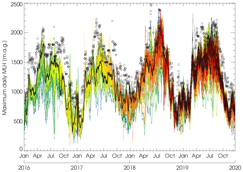
Figure 9 Maximum daily mixing layer height a.g. (MMLH) observed by the German ceilometers and extracted from the ECMWF NWP model for the period January 2016–December 2019. Different colors refer to model MMLH at different stations (colors shift from green to red because the number of stations increases over the years). The dots and the solid black line pick out the MMLH inferred around Alfeld (52.0^∘ N, 9.9^∘ E) manually from the daily ceilometer time–height plots and from the model fields, respectively.

In the presence of large variability, the model generally underestimates the MMLH by −200 to −600 m in 2016 and 2017, by 0 to −300 m with cycle 43r3 after October 2017 and is biased low between −200 and −500 m during cycle 46r1 after July 2019. In Fig. 10, a composite contour-bullet plot of IFS MLH with superimposed station values from 20 March 2019 illustrates the behavior of MMLH for a calm day with undisturbed ML development over large parts of Germany. Here, IFS-AER is able to reproduce the NW-to-SE increase of the MMLH related to the transit from low to higher pressure. Few stations sticking out with specifically high or low MMLH probably exhibit local influence like heat-island effects over large cities (e.g., “lei” indicates Leipzig), where the residual layer remained high and convective during the night. Over isolated mountains (e.g., Brocken/Torfhaus – the deep blue dot near 51^∘ N, 10.5^∘ E), the ML top may not follow the steep terrain and local MLH above ground will be too low. It turns out that rigid checks of station characteristics, data quality and outliers are necessary before operational MLH data from ceilometers (or lidars) may be used to constrain and evaluate models.

Figure 10 Map of maximum daily MLH as simulated by IFS-AER (filled contours) with MMLH at German ceilometer network stations for 20 March 2019, overlain as correspondingly color-coded bullets.

4.2 Uncertainties and limitations

The overall uncertainty of our results is mainly limited by the conversion of model mass mixing ratios to β^∗(z), the uncertainty of the ceilometer observations and the resampling over different horizontal and vertical resolutions. The former includes estimates of particle shape, densities, mixing and hygroscopic state, as well as meteorological conversions as described in Chan et al. (2018) and updated in Sect. 2.1. The uncertainties inherent in the observations are discussed in Sect. 2.2. Of these, clearly the lower and upper altitude ranges of the profiles are affected by the incomplete overlap of laser-beam and receiver field of view and low SNR as well as contamination by clouds, respectively. At the lowest considered altitude (400 m a.g.), the signal is typically at ∼ 10 %–20 % of its full-overlap value, which can reasonably be corrected by a sin²-like step function. The crucial degradation of the SNR is a result of clouds, precipitation and the r⁻² decrease with distance. Within the evaluated range from 0.4–6 km, however, the combined uncertainty due to these contributions mostly is small compared to the model–observation biases in question. Due to the typical half-daily timescale of transport precision (cf. Sect. 3.2), also the distance from the model grid points seems negligible. Many of the results, however, are sensitive to the applied scales, and some examples have been discussed where the increased horizontal (June 2018) and vertical (July 2019) resolution led to better matches between observed and forecast structures. It has to be kept in mind that the relatively coarser global fields of the CAMS system are intended to serve as boundary conditions for nested regional models which refine the aerosol distributions down to scales of a few kilometers.

As there was no β^∗(z) output available from IFS-AER before cycle 45r1 (October 2017), for consistency, we use the same lidar forward operator over the whole period to calculate β^∗(z) from the model mass mixing ratios, as described in Chan et al. (2018). Minor modifications were necessary to integrate the higher resolution and additional species (NO₃, NH₄) as of July 2019. It uses their precalculated look-up table, slightly adapted to IFS-AER values and modified to additionally handle NO₃ and NH₄ (cf. Tables C1–C3). Since October 2017, lidar output has been available from the IFS archive. Results from both emulators compare well for dust, but for other components like sea salt somewhat different β^∗(z) profiles are calculated. Possible reasons may be the handling of hygroscopic growth near saturation, the disregard of (however small) absorption by trace gases at 1064 nm and a different effective resolution of the model fields resulting from both lidar emulators. A direct comparison of the β^∗(z) (from ground) product retrieved from the IFS and that calculated from the model mass mixing ratios according to Chan et al. (2018) reveals that the IFS β^∗(z) product is provided with a different effective resolution then the mmr fields used here. The gradients thus appearing at the boundaries of aerosol structures cause deviating results depending on the specific time and location of the comparison. For longer averages, as mostly discussed in this article, these differences largely cancel out.

5 Summary

The assessment of IFS-AER vertical aerosol distributions with calibrated ceilometer profiles over Germany (central Europe) generally confirms the realistic reproduction of the vertical aerosol variability in terms of attenuated backscatter β^∗(z). The shape of the profile, dominated by the ML and occasionally by long-range transport particles, is largely captured, as indicated by high covariance of daily average profiles with Pearson's r≈0.6–0.95; however, no clear impact of the assimilation is found. In summer, the agreement of profile shapes is worse due to vertical shifts or untimely long-range transport to which r is quite sensitive. A systematic high- or low-bias regularity is found in the lower part of the profile, meaning a high bias (overestimation) near the ground versus low bias in the mixing layer. It is attributed to overestimated sources at the surface, likely in combination with too-slow vertical transport and probably a too-weak transport barrier at the top of the ML, where the large aerosol gradient is not fully captured. The low aerosol background in the FT is usually reproduced. Also captured are plumes and layers from long-range transport of Saharan dust and fire smoke, although β^∗(z) of dust is overestimated over Germany by a factor of 2 or more, and small-scale structures evolving during the dispersion of these layers cannot be resolved at the present model resolution.

Comparison to dry-state aerosol in situ observations suggests that SO₄ and OM sources as well as gas-to-particle partitioning of the NO₃–NH₄ system are too strong, while black carbon load and trend are realistic near the surface. With respect to the discussed metrics, no consistent development is evident due to the five model upgrades during the evaluated period. The vertically integrated β^∗(z), which codes similar information to AOD, consistently with these previous findings shows a bias near zero for cycles 43r1 (until May 2016) and 46r1 (after July 2019) and slightly negative in between. The MNMB, which is less dependent on absolute values, reveals lower values in the more relevant (for air quality) surface and mixing layer and a general increase toward higher levels. Over the whole period, the bias of β^∗(z) exhibits seasonal cycles at the lower levels due to overestimation of SO₄ and OM sources/lifetimes in summer and under-representation of severe pollution episodes in winter.

Finally, we demonstrated that ceilometer networks offer several options to check the realism of mixing layer heights in atmospheric numerical models. Though we confined to manual analysis of a representative region, we could provide confidence that the annual cycle and the maximum daily height of the ML can be reproduced within several hundred meters vertically by the IFS-AER model.

In the future, the regional extension of this assessment to larger parts of Europe and the combination of ceilometer networks' spatiotemporal coverage with the higher accuracy and particle identification capability of Sun photometers (AERONET) and multi-wavelength depolarization (Raman) lidars will significantly reduce the uncertainties remaining in this study. Complementing CAMS activities, also for evaluation of the particle composition using European in situ network data, have already started. A robust discussion of boundary layer heights will benefit more from further improvements to the algorithms than from improved profile data quality.

Appendix A: Attenuated backscatter from model mass mixing ratios – forward operator

A forward operator is applied to translate the model state of the atmosphere into virtual measurements, which can be directly compared to real observations. To this end, model mmr values are converted to attenuated backscatter β^∗(z) according to Eq. (1) by first calculating mass concentrations c_p,i from mmr by multiplication with the air density ϱ_air as shown in Eq. (A1).

$$\begin{array}{}\text{(A1)}& c_{\mathrm{p},i}\left(z\right)={\mathit{\varrho }}_{\mathrm{air}}\left(z\right)m_{\mathrm{p},i}\left(z\right)\text{for}i=\mathrm{1},\mathrm{2},\mathrm{\dots },\mathrm{14}\end{array}$$

Then the particle extinction coefficient σ_p,i and the particle backscatter coefficient β_p,i of each particle type i have been precalculated using appropriate particle size distributions d$N\left(r\right)/$dr and humidity-dependent particle refractive indices n as applied in IFS-AER (Chan et al., 2018). For consistency with the current implementation of the aerosols in the IFS model, Mie scattering theory has been applied for all particles. Model mass concentrations are then converted to extinction coefficients by means of the specific (mass) extinction coefficient ${\mathit{\sigma }}_{\mathrm{e},i}^{*}$ (unit: m²/g).

$$\begin{array}{}\text{(A2)}& {\mathit{\sigma }}_{\mathrm{e},i}^{*}={\displaystyle \frac{{\mathit{\sigma }}_{\mathrm{p},i}}{c_{\mathrm{p},i}}}\end{array}$$

Equation (A2) is applied separately to each size and humidity bin of the humidity-dependent and size-segregated particle types. For convenience, the lidar ratio S_p,i is commonly used to calculate particle backscatter coefficients from extinction coefficients.

$$\begin{array}{}\text{(A3)}& S_{\mathrm{p},i}\left(z\right)={\displaystyle \frac{{\mathit{\sigma }}_{\mathrm{p},i}\left(z\right)}{{\mathit{\beta }}_{\mathrm{p},i}\left(z\right)}}\end{array}$$

With this definition, the extinction and backscatter coefficients of each particle type are determined from Eqs. (A4), (A5).

$$\begin{array}{}\text{(A4)}& {\displaystyle }{\mathit{\sigma }}_{\mathrm{p},i}=c_{\mathrm{p},i}{\mathit{\sigma }}_{\mathrm{e},i}^{*}\text{(A5)}& {\displaystyle }{\mathit{\beta }}_{\mathrm{p},i}=c_{\mathrm{p},i}\left({\displaystyle \frac{{\mathit{\sigma }}_{\mathrm{e},i}^{*}}{S_{\mathrm{p},i}}}\right)\end{array}$$

The contribution from air molecules is calculated according to Rayleigh theory using the following approximation for the molecular extinction coefficient σ_m (in km⁻¹):

$${\mathit{\sigma }}_{\mathrm{m}}(z,\mathit{\lambda })=\mathrm{8.022}\times {\mathrm{10}}^{-\mathrm{4}}{\mathit{\varrho }}_{\mathrm{air}}\left(z\right){\mathit{\lambda }}^{-\mathrm{4.08}},$$

with the air density given in kg/m³ and the wavelength λ in  µm. The profile of ϱ_air is taken from the IFS. The molecular lidar ratio S_m is known to be $S_{\mathrm{m}}={\mathit{\sigma }}_{\mathrm{m}}/{\mathit{\beta }}_{\mathrm{m}}=\mathrm{8}\mathit{\pi }/\mathrm{3}$. To increase computational efficiency, the precalculated values of ${\mathit{\sigma }}_{\mathrm{e},i}^{*}$, S_p,i(z) as well as ϱ_air are stored in a look-up archive, as displayed in Tables C1–C3. In order to calculate the total β^∗(z), according to Eq. (A6), the contributions from all particle types are summed up to yield the (total) backscatter coefficient:

$$\mathit{\beta }={\mathit{\beta }}_{\mathrm{m}}+\sum _{i=\mathrm{1}}^{\mathrm{14}}{\mathit{\beta }}_{\mathrm{p},i}.$$

Finally, the attenuation is applied to β(z) to calculate β^∗(z):

$$\begin{array}{}\text{(A6)}& {\mathit{\beta }}^{\ast }\left(z\right)=\mathit{\beta }\left(z\right)\exp \left\{-\mathrm{2}\underset{\mathrm{0}}{\overset{z}{\int }}\mathit{\sigma }\left(z^{\prime }\right)\mathrm{d}{z}^{\prime }\right\}.\end{array}$$

Appendix B: Cloud formation due to SD

Though Saharan dust transport is realistic in IFS-AER on spatiotemporal scales >100 km and >0.5 d, the dust load is mostly overestimated. Occasionally, however, β^∗(z) of dust plumes is apparently underestimated because dust particles rapidly grow by water uptake and observed β^∗(z) changes though the dust mass concentration itself remains constant. Though the ability of (coated) mineral dust to foster cloud formation is well known, its simulation is still a challenge (Sassen et al., 2003; Ansmann et al., 2005; Bangert et al., 2012). For example, on 16 and 17 October 2017, a Saharan dust plume swayed eastward over northwestern Germany, shown in detail for Aachen in Fig. B1. On both days, similar dust loads, converted to similar β^∗(z), are simulated by the model, but on 16 October observed β^∗(z) values were as usual less than half of those modeled, while on 17 October hygroscopic growth or incipient cloud formation temporarily multiplied the optical signal 10-fold (${\mathit{\beta }}^{\ast }(z{)}_{max}=\mathrm{1.2}\times {\mathrm{10}}^{-\mathrm{5}}$ Mm⁻¹ sr⁻¹), while the dust mass concentration according to the continuity of the β^∗(z) signal and its development a few hours later and its development at neighboring stations did not change (Fig. B2). As hygroscopic growth is included in the IFS-AER model but cloud formation by condensation nuclei is not, this process may significantly distort average biases of β^∗(z) during SDDs as well as precipitation and radiation transfer (indirect aerosol effect) in the model. It further illustrates how errors may be introduced by conversions of the primary model parameters (mass mixing ratio) to observed β^∗(z). On 17 October 2017, also biomass burning aerosol released by forest fires in the north of Portugal was observed over north Germany as a shallow layer descending from initially 8–10 km (∼ 03:00 UTC at Putbus) to 4–5 km altitude around noon. Observed β^∗(z) ranges from 0.1–$\mathrm{1}\times {\mathrm{10}}^{-\mathrm{5}}$ Mm⁻¹ sr⁻¹. At the time of incipient cloud formation, this layer still was clearly separated from the Saharan dust layer below and thus could not influence this process.

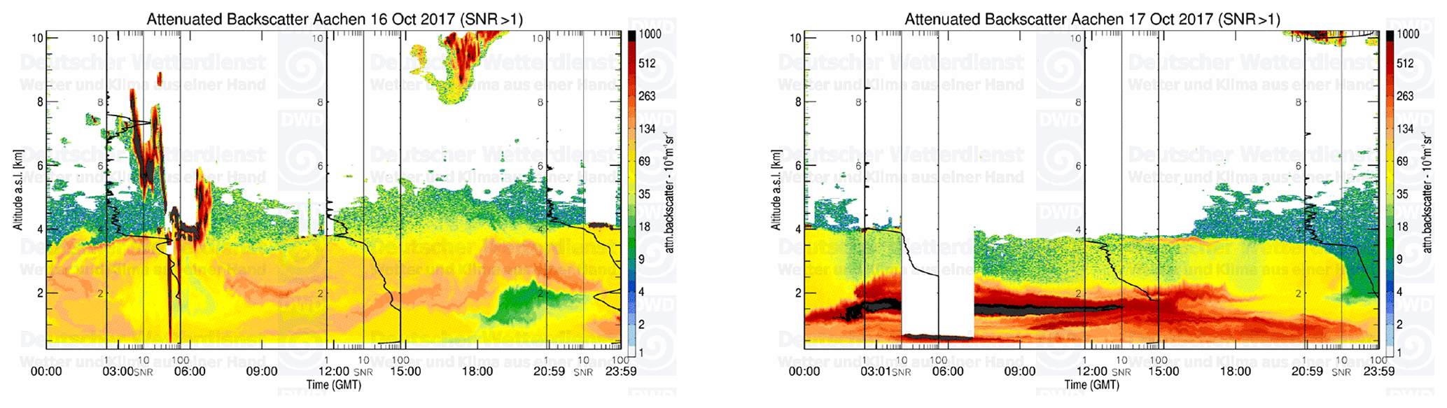
Figure B1 Time–height sections of β^∗(z) at the ceilometer station near Aachen from 16 and 17 October 2017.

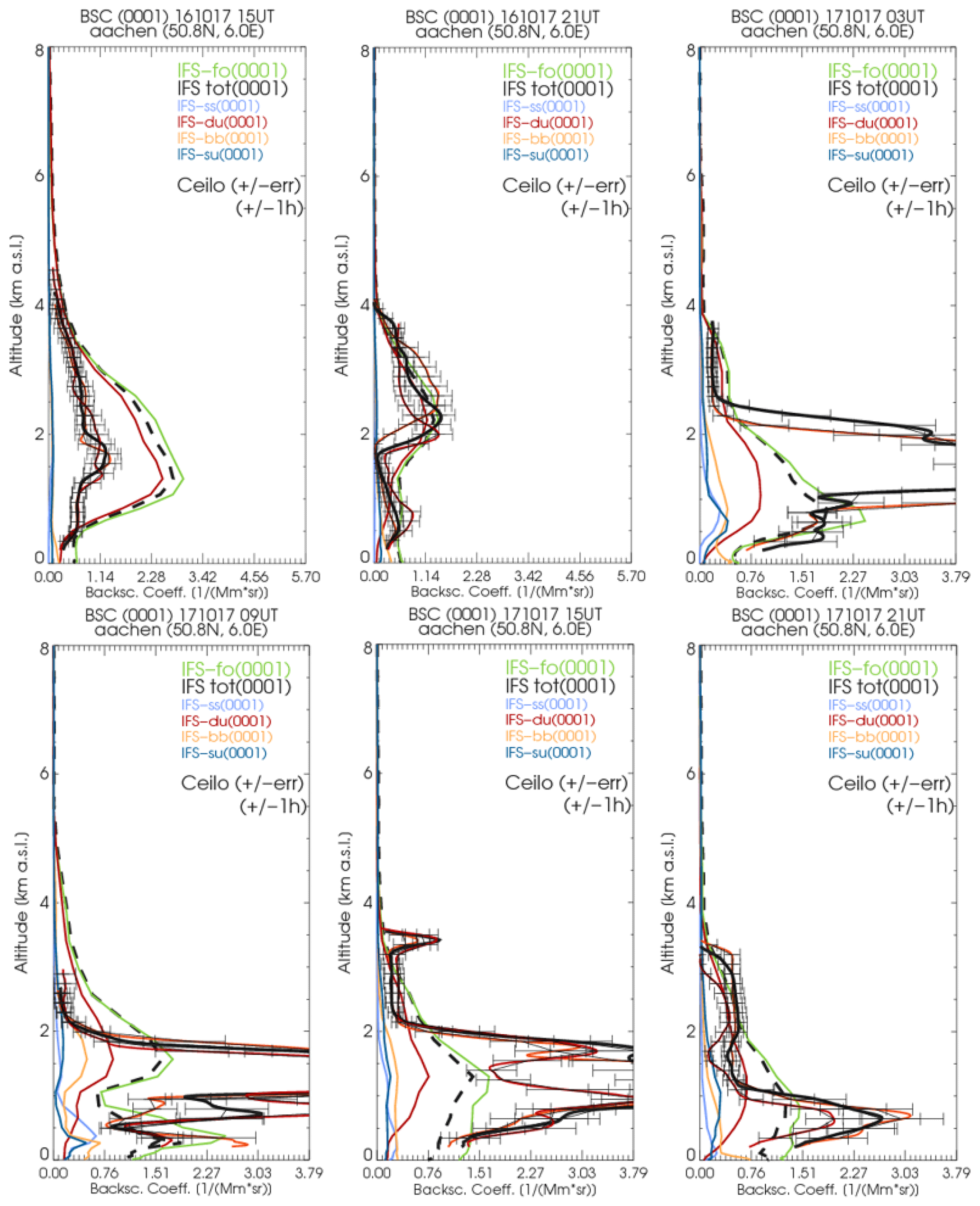
Figure B2 Profiles of β^∗(z) from the ceilometer near Aachen on 16 (15:00, 21:00 UTC) and 17 (03:00, 09:00, 15:00, 21:00 UTC) October 2017 from IFS-AER and ceilometer. The dashed black line is calculated with the DWD forward operator (FO); the green line is calculated using the ECMWF FO, retrieved as “attenuated backscatter from ground” from the MARS archive. Onset of cloud formation occurs in the SD air mass on early 17 October. Colored profiles show the contributions of individual aerosol types.

Appendix C: Look-up tables for forward operator

The aerosol optical and microphysical properties used for converting model mmr values to attenuated backscatter β^∗(z) (the “forward operator” or “lidar emulator”) are listed in the following tables. Values refer to 1064 nm used by CHM15k ceilometers.

Table C1 Microphysical properties of aerosols assumed for conversion of model mass mixing ratios to β^∗(z) at 1064 nm.

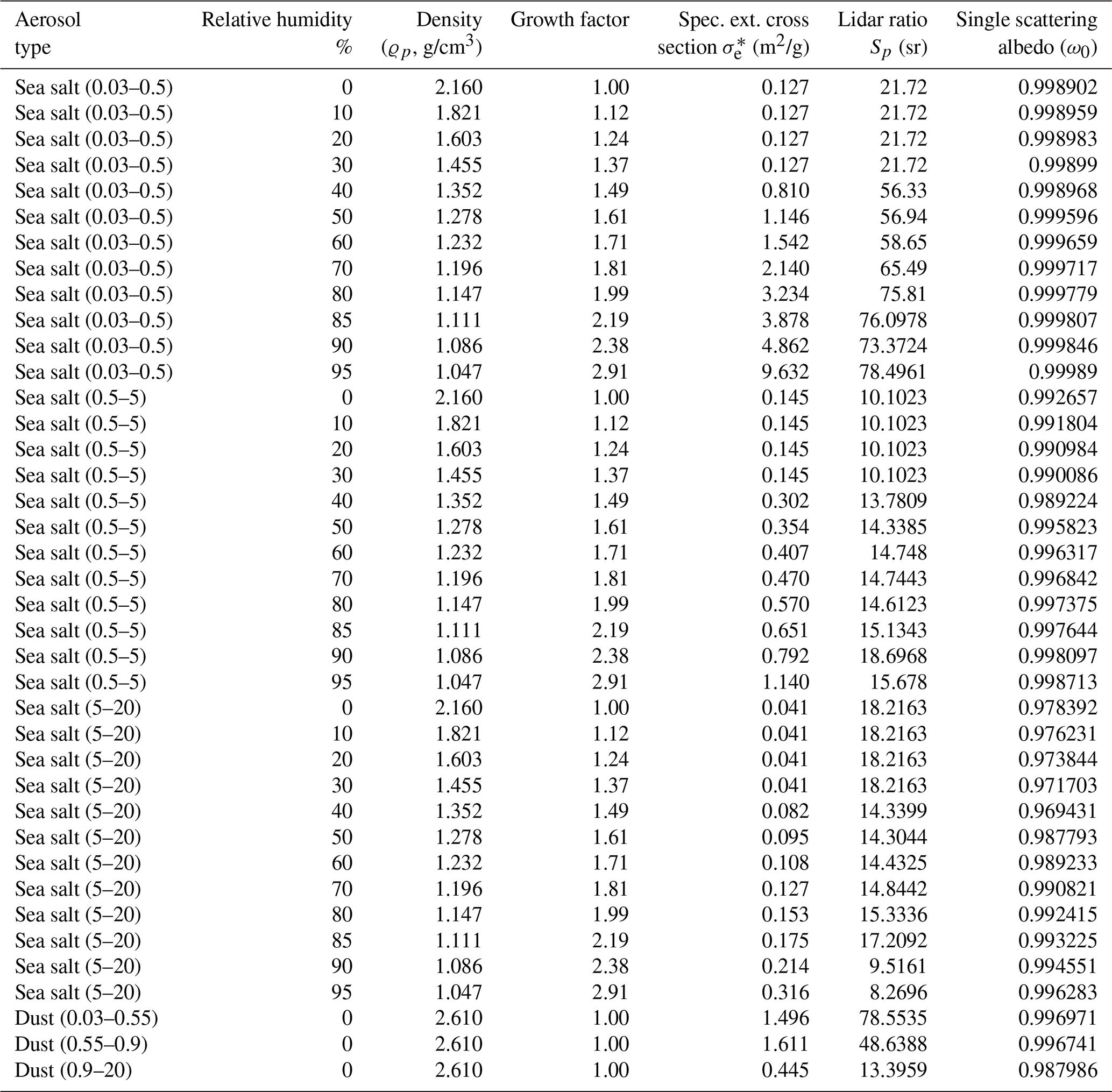
(a) Sea-salt aerosols are represented in the model by three size bins with bin limits set to 0.03–0.5 µm (bin 1), 0.5–5 µm (bin 2) and 5–20 µm (bin 3). (b) Dust aerosols are represented in the model by three size bins with bin limits set to 0.03–0.55 µm (bin 1), 0.55–0.90 µm (bin 2) and 0.90–20.00 µm (bin 3). (c) A bimodal log-normal size distribution is assumed for sea-salt aerosols, with r₀=0.1002 and 1.002 µm and σ_g=1.9 and 2.0. A monomodal size distribution is assumed for dust. The number concentrations N₁ and N₂ of the first and second modes are 70 and 3 cm⁻¹, respectively. Note that density of hydrophilic aerosol changes with the hygroscopic growth of particles.

Table C2 Microphysical properties of aerosols assumed for conversion of model mass mixing ratios to β^∗(z) at 1064 nm.

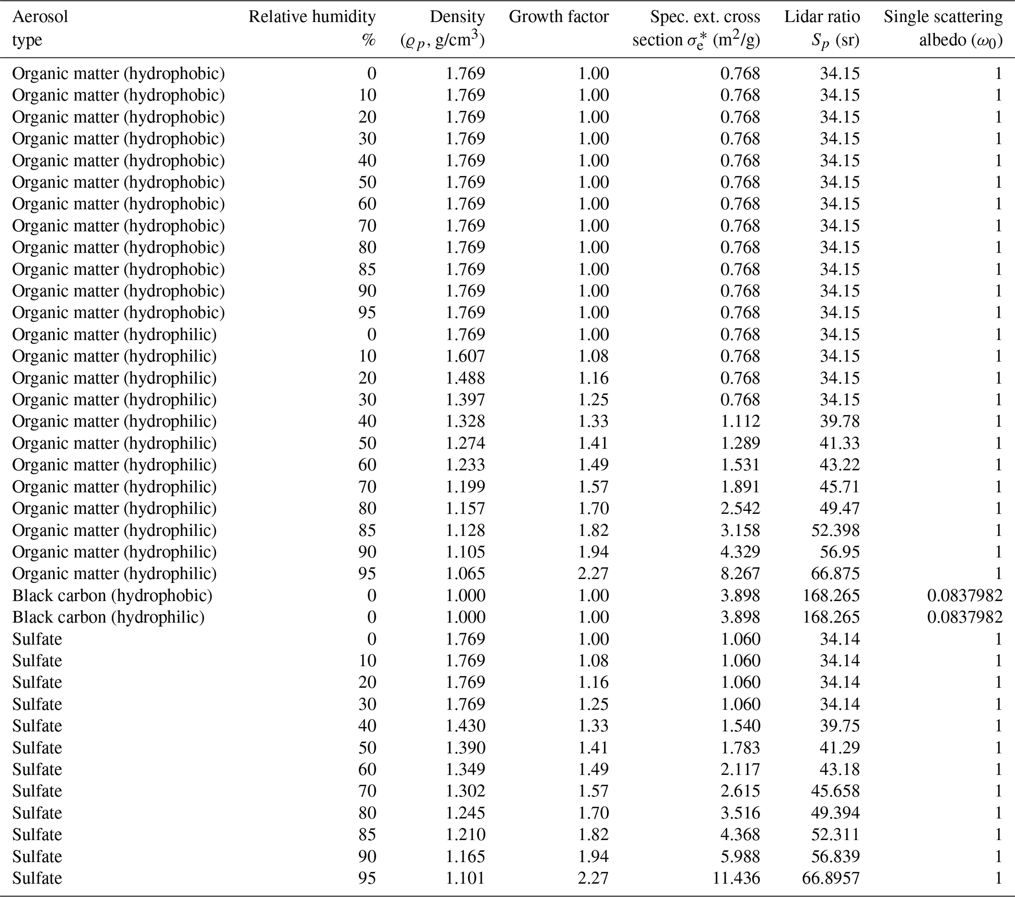
Table C3 Microphysical properties of aerosols assumed for conversion of model mass mixing ratios to β^∗(z) at 1064 nm.

Appendix D: Monthly mean profiles

In order to illustrate the shapes of the actual vertical β^∗(z) profiles from the model (ASM and CTR) and the ceilometers, the 48 individual monthly average profiles are given in Figs. D1, D2, D3 and D4.

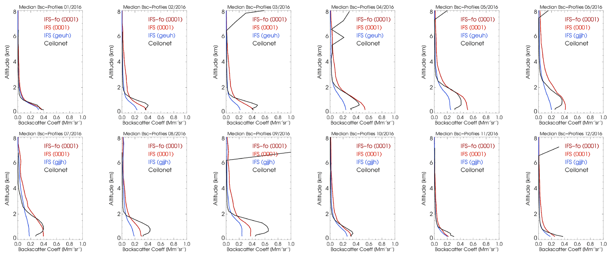
Figure D1 Monthly median profiles 2016 from the ceilometer (black), ASM (red) and control run (blue).

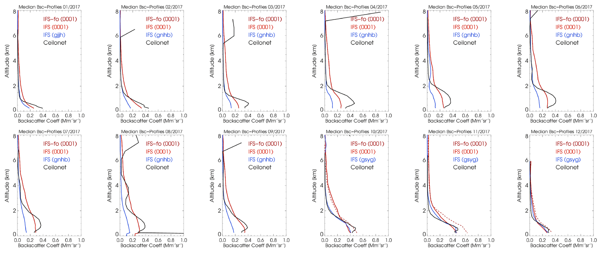
Figure D2 Monthly median profiles 2017 from the ceilometer (black), ASM (red) and control run (blue). The median profile from the IFS forward operator is added as a dashed red line.

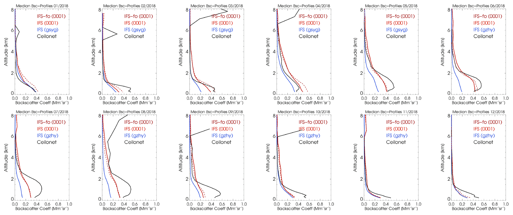
Figure D3 Monthly median profiles 2018 from the ceilometer (black), ASM (red) and control run (blue). The median profile from the IFS forward operator (available as of October 2017) is added as a dashed red line.

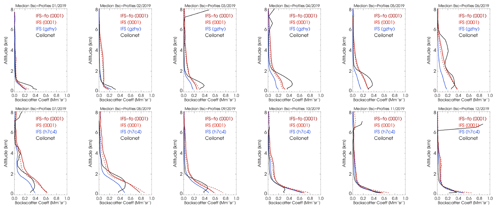
Figure D4 Monthly median profiles 2019 from the ceilometer (black), ASM (red) and control run (blue). The median profile from the IFS forward operator is added as a dashed red line.