the Creative Commons Attribution 4.0 License.
the Creative Commons Attribution 4.0 License.
 | 15 Mar 2021
On the suitability of second-order accurate finite-volume solvers for the simulation of atmospheric boundary layer flow
Beatrice Giacomini
The present work analyzes the quality and reliability of an important class of general-purpose, second-order accurate finite-volume (FV) solvers for the large-eddy simulation of a neutrally stratified atmospheric boundary layer (ABL) flow. The analysis is carried out within the OpenFOAM® framework, which is based on a colocated grid arrangement. A series of open-channel flow simulations are carried out using a static Smagorinsky model for subgrid scale momentum fluxes in combination with an algebraic equilibrium wall-layer model. The sensitivity of the solution to variations in numerical parameters such as grid resolution (up to 1603 control volumes), numerical solvers, and interpolation schemes for the discretization of nonlinear terms is evaluated and results are contrasted against those from a well-established mixed pseudospectral–finite-difference code. Considered flow statistics include mean streamwise velocity, resolved Reynolds stresses, velocity skewness and kurtosis, velocity spectra, and two-point autocorrelations. A quadrant analysis along with the examination of the conditionally averaged flow field are performed to investigate the mechanisms responsible for momentum transfer in the flow. It is found that at the selected grid resolutions, the considered class of FV-based solvers yields a poorly correlated flow field and is not able to accurately capture the dominant mechanisms responsible for momentum transport in the ABL. Specifically, the predicted flow field lacks the well-known sweep and ejection pairs organized side by side along the cross-stream direction, which are representative of a streamwise roll mode. This is especially true when using linear interpolation schemes for the discretization of nonlinear terms. This shortcoming leads to a misprediction of flow statistics that are relevant for ABL flow applications and to an enhanced sensitivity of the solution to variations in grid resolution, thus calling for future research aimed at reducing the impact of modeling and discretization errors.
- Article
(6037 KB) - Full-text XML
- BibTeX
- EndNote


An accurate prediction of atmospheric boundary layer (ABL) flows is of paramount importance across a wide range of fields and applications, including weather forecasting, complex terrain meteorology, agriculture, air quality modeling, and wind energy (Whiteman, 2000; Fernando, 2010; Calaf et al., 2010; Oke et al., 2017; Shaw et al., 2019).
Since the early work of Deardorff (1970), the large-eddy simulation (LES) technique has spurred considerable insight on the fundamental dynamics of ABL flow over rough surfaces (Anderson and Meneveau, 2010; Salesky et al., 2017; Momen et al., 2018), over and within plant and urban canopies (Yue et al., 2007b; Bailey and Stoll, 2013; Pan et al., 2014; Tseng et al., 2006; Bou-Zeid et al., 2009; Giometto et al., 2017; Li and Bou-Zeid, 2019), and for wind energy applications (Calaf et al., 2010; Abkar and Porté-Agel, 2013; Stevens and Meneveau, 2017), amongst others.
The majority of the past work has relied on fully or partially dealiased mixed pseudospectral–finite-difference (PSFD) solvers – the go-to approach for LES studies since the works of Moin et al. (1978) and Moeng (1984). Such solvers are known to yield accurate flow fields up to the LES cutoff frequency and to produce good results when used in conjunction with dynamic subgrid scale (SGS) models (Germano et al., 1991; Lilly, 1992). However, single domain PSFD-based solvers are limited to regular domains, are not suitable for the simulation of nonperiodic flows, have sharp variations in the flow field such as shocks or fluid–solid interfaces in boundary layer flows, and are typically difficult to parallelize owing to the global support of their spatial representation (see, e.g., Margairaz et al., 2018). With the increasing need to account for complex geometries and multiphysics, several efforts have been devoted to the mitigation of the aforementioned limitations (Fang et al., 2011; Li et al., 2016; Chester et al., 2007). However, the solutions are often ad hoc or validated only for specific applications, thus introducing a degree of uncertainty in model results that is hard to quantify and generalize.
There is hence a growing interest from the ABL community in LES solvers based on compact spatial schemes via structured or unstructured meshes (Orlandi, 2000; Ferziger and Peric, 2002). The parallelized large-eddy simulation model (Raasch and Schröter, 2001; Maronga et al., 2015) and the weather research and forecasting model (Skamarock and Klemp, 2008; Powers et al., 2017) are prominent examples of said efforts. Both the approaches are based on a high-order finite-difference discretization, with nonlinear terms approximated by using high-order upwind biased differencing schemes. The latter are suitable for LES in complex geometries with arbitrary grid stretching factors and outflow boundary conditions (Beaudan and Moin, 1994; Mittal and Moin, 1997) but are dissipative and do not strictly conserve energy. On the other hand, if central schemes are used instead for the evaluation of nonlinear terms, no numerical dissipation is introduced, but truncation errors can have an overwhelming impact on the computed flow field (Ghosal, 1996; Kravchenko and Moin, 1997). These limitations typically result in a strong sensitivity of the solution to properties of the spatial discretization and numerical scheme (Meyers et al., 2006, 2007; Meyers and Sagaut, 2007; Vuorinen et al., 2014; Rezaeiravesh and Liefvendahl, 2018; Breuer, 1998; Montecchia et al., 2019). Further, truncation errors corrupt the high wavenumber range of the solution, restricting the ability to adopt dynamic LES closure models that make use of information from the smallest resolved scales of motion to evaluate the SGS diffusion (Germano et al., 1991). Notwithstanding these limitations, central schemes have been heavily employed in the past in both the geophysical and engineering flow communities and are the de facto standard in the wind engineering community, where most of the numerical simulations are carried out using second-order accurate finite-volume (FV)-based solvers (Stovall et al., 2010; Churchfield et al., 2010; Balogh et al., 2012; Churchfield et al., 2013; Shi and Yeo, 2016, 2017; García-Sánchez et al., 2017; García-Sánchez and Gorlé, 2018).
Motivated by the aforementioned needs, the present study aims at characterizing the quality and reliability of an important class of second-order accurate FV solvers for the LES of neutrally stratified ABL flows. The analysis is conducted in the open-channel flow setup (no Coriolis acceleration) via the OpenFOAM® framework (Weller et al., 1998; De Villiers, 2006; Jasak et al., 2007). A suite of simulations is carried out varying physical and numerical parameters, including grid resolution (up to 1603 control volumes), the numerical solver, and interpolation schemes for the discretization of the nonlinear term. Predictions from the FV solvers are contrasted against the results from the Albertson and Parlange (1999) PSFD code in terms of flow statistics, including mean streamwise velocity, resolved Reynolds stresses, two-point velocity autocorrelations, and mechanisms supporting momentum transport. The end goal is to provide a more nuanced understanding of the capabilities of general-purpose, second-order, FV-based solvers in predicting ABL flow.
The work is organized as follows. Section 2 summarizes the setup of the problem, the simulation database, and the postprocessing procedure. Results are shown in Sect. 3 and conclusions are drawn in Sect. 4. A further discussion on the sensitivity of the solution to model constants, interpolation schemes, and numerical solvers is provided in the Appendix.
2.1 Governing equations and numerical schemes
We use index notation in a Cartesian reference system. The spatially filtered Navier–Stokes equations are considered,
where is the spatially filtered velocity field along the streamwise (x), cross-stream (y), and vertical (z) coordinate directions, respectively, t is the time, ρ is the constant fluid density (Boussinesq approximation), is a modified pressure term, τij is the filtered viscous stress tensor, and is the deviatoric part of the SGS stress tensor. In addition, the term is an imposed constant pressure gradient driving the flow. The spatially filtered viscous tensor is , where ν=const is the kinematic viscosity of the Newtonian fluid and Sij is the resolved (in the LES sense) rate of strain tensor. For the SGS stress tensor, the static Smagorinsky model is used,
where νSGS is the SGS eddy viscosity, CS is the Smagorinsky coefficient (Smagorinsky, 1963), is a local length scale based on the volume of the computational cell (Scotti et al., 1993), and quantifies the magnitude of the rate of strain. In the present work, CS=0.1, unless otherwise specified. Note that dynamic Smagorinsky models are preferred to the static one for the LES of ABL flows (Germano et al., 1991; Lilly, 1992; Meneveau and Lund, 1997; Porté-Agel, 2004; Bou-Zeid et al., 2005). Dynamic models evaluate SGS stresses via first-principles-based constraints, feature improved dissipation properties when compared to the static Smagorinsky model (especially in the vicinity of solid boundaries), and are free of explicit modeling parameters. The choice made in the present study is motivated by problematics encountered when using the available dynamic Lagrangian model in preliminary tests. However, while SGS dissipation plays a crucial role in PSFD solvers, truncation errors may overshadow SGS stress contributions in the second-order FV-based ones (Kravchenko and Moin, 1997). The static Smagorinsky SGS model used herein might hence perform similarly to dynamic SGS models for the considered flow setup. This conjecture is supported by the results of Majander and Siikonen (2002).
The large scale separation between near-surface and outer-layer energy-containing ABL motions poses stringent resolution requirements to numerical modelers, if all the energy containing motions have to be resolved. To reduce the computational cost of such simulations, the near-surface region is typically bypassed and a phenomenological wall-layer model is leveraged instead to account for the impact of near-wall (inner-layer) dynamics on the outer-layer flow (Piomelli, 2008; Bose and Park, 2018). This approach is referred to as wall-modeled large-eddy simulation (WMLES) and is used herein. An algebraic wall-layer model for surfaces in a fully rough aerodynamic regime was implemented based on the logarithmic equilibrium assumption, i.e.,
where is the norm of the velocity at a certain distance from the ground level, u* is the friction velocity (see Sect. 2.2 for details), κ is the von Kármán constant, z is the distance from the ground level, and z0 is the so-called aerodynamic roughness length, a length scale used to quantify the drag of the underlying surface. In this work, the values κ=0.41 and z0=0.1 m are set. The kinematic wall shear stress is assumed to be proportional to the local velocity gradient (Boussinesq hypothesis),
where νt is the total eddy viscosity. Employing the no-slip condition for the velocity field, the standard FV approximation of the shear stress at the wall gives (Mukha et al., 2019)
where the subscript f is used to denote the evaluation at the center of the wall face, the subscript c denotes the evaluation at the center of the wall-adjacent cell, and Δz is the distance from the wall. From the logarithmic law (Eq. 4) evaluated at the first cell center, one can write . Using the definition of friction velocity , where τw is the magnitude of the kinematic wall shear stress vector, along with Eq. (5), and rearranging, the total eddy viscosity at the wall can be written as
which is the formulation implemented herein. Note that in the boundary layer flows in the fully rough aerodynamic regime, so ν could be neglected without loss of accuracy.
In the present work, the computational grid is colocated, being the only colocated grid arrangement available within the OpenFOAM® framework. Note that although advantageous in complex domains when compared to staggered grids (Ferziger and Peric, 2002), the colocated arrangement is known to cause difficulties with pressure–velocity coupling, hence requiring specific procedures to avoid oscillations in the solution. OpenFOAM® offers the standard Rhie–Chow correction (Rhie and Chow, 1983), which is known to negatively affect the energy-conservation properties of central schemes (Ferziger and Peric, 2002). In addition, when approximating the integrals over the surfaces bounding each control volume (as a consequence of the Gauss divergence theorem), the unknowns are evaluated at face centers and are assumed to be constant at each face, yielding an overall second-order spatial accuracy (Churchfield et al., 2010). Since the divergence form of the convective term is used in combination with a low-order scheme over a nonstaggered grid, the solution is inherently unstable (Kravchenko and Moin, 1997). The present work makes use of the linear and QUICK interpolation schemes (Ferziger and Peric, 2002) to evaluate the unknowns at face centers (more details are provided in Sect. 2.2). The numerical solver is based on the PISO algorithm (Issa, 1985) for the pressure–velocity calculation and on an implicit Adams–Moulton scheme for time integration (Ferziger and Peric, 2002). In Appendix A2, the performances of an alternative solver with a Runge–Kutta time-advancement scheme and a projection method for the pressure–velocity coupling (Vuorinen et al., 2014) are analyzed.
2.2 Problem setup
A series of WMLES of ABL flow (open-channel flow setup) is performed. Tests are carried out in the domain with Lx=2πh, , Lz=h, where h=1000 m denotes the width of the open channel. Symmetry is imposed at the top of the computational domain, no-slip applies at the lower surface, and periodic boundary conditions are enforced along each side. A kinematic pressure gradient term drives the flow along the x coordinate direction, yielding . The kinematic viscosity is set to a nominal value of , which results in an essentially inviscid flow.
The computational mesh is Cartesian, with a uniform stencil along each direction. Three simulations are run over 643, 1283, and 1603 control volumes, with the linear interpolation scheme for the evaluation of the unknowns at the face centers (simulations FV64, FV128, and FV160, respectively). Three additional simulations are run, at the same grid resolutions, with the linear scheme for the approximation of every term except for the nonlinear one, for which the QUICK scheme is used instead (simulations FV64*, FV128*, and FV160*). The cases span different grid resolutions at the same aspect ratio . Note that the chosen grid resolutions are in line with those typically used in studies of ABL flow with the pseudospectral approach (see, e.g., Salesky et al., 2017). All the calculations satisfy the Courant–Friedrichs–Lewy (CFL) condition C≲0.1, where C is the Courant number. Runs are initialized from a fully developed open-channel flow simulation in statistically steady state (dynamic equilibrium), and time integration is carried out for 100 eddy turnover times, where the eddy turnover time is defined as . Flow statistics are the result of an averaging procedure over the horizontal plane of statistical homogeneity of turbulence (xy) and in time over the last 60 eddy turnover times. The procedure yields well-converged statistics throughout the considered cases. In the following, the horizontal and temporal averaging operation is denoted by 〈⋅〉. The results from the present study are contrasted against the corresponding ones from the Albertson and Parlange (1999) mixed PSFD code (simulations PSFD64, PSFD128, and PSFD160). The code is based on an explicit second-order accurate Adams–Bashforth scheme for time integration and on a fractional-step method for solving the system of equations. Simulations from the PSFD solver are carried out using a static Smagorinsky SGS model with CS=0.1, a rough wall-layer model with z0=0.1 m, and C≲0.1. A summary of the runs is given in Table 1 along with the acronyms used in this study.

This section is devoted to the analysis of velocity central moments (Sect. 3.1), spectra and spatial autocorrelations (Sect. 3.2), and momentum transfer mechanisms (Sect. 3.3).
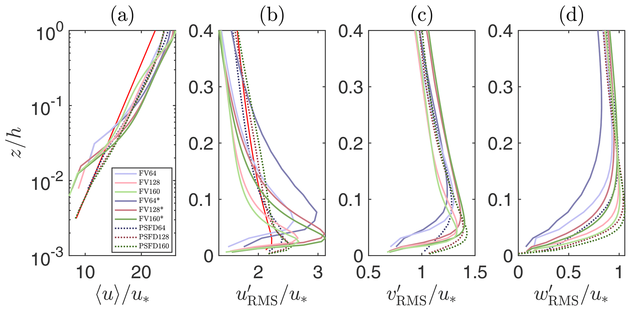
Figure 1Vertical structure of mean streamwise velocity (a), streamwise velocity RMS (b), cross-stream velocity RMS (c), and vertical velocity RMS (d). The red line in (a) denotes the reference logarithmic profile and the red line in (b) is a reference profile from Hultmark et al. (2013).
3.1 Mean velocity, Reynolds stresses, and higher-order statistics
Figure 1 shows first- and second-order statistics for all the considered cases. The mean streamwise velocity is shown in Fig. 1a in a comparison with the phenomenological logarithmic-layer profile. The velocity at the first two cell centers off the wall is consistently underpredicted, whereas a positive log-layer mismatch (LLM) is observed in the bulk of the flow (Kawai and Larsson, 2012). The LLM is particularly pronounced for the cases using the QUICK interpolation scheme. This behavior could have been anticipated, as the wall shear stress is evaluated using the instantaneous horizontal velocity at the first cell center off the wall. A number of procedures has been proposed to alleviate the LLM, including modifying the SGS stress model in the near-wall region (Sullivan et al., 1994; Porté-Agel et al., 2000; Chow et al., 2005; Wu and Meyers, 2013), shifting the matching location further away from the wall (Kawai and Larsson, 2012), and carrying out a local horizontal/temporal filtering operation (Bou-Zeid et al., 2005; Xiang et al., 2017). In preliminary runs, the approach of Kawai and Larsson (2012) was implemented in an attempt to alleviate the LLM. However, no apparent improvement was observed and the solution became very sensitive to grid resolution and matching location. This finding suggests that alternative procedures might need to be devised to overcome the LLM in ABL flow simulations when using the considered class of FV solvers. Note that profiles from the PSFD solver also feature a positive LLM in spite of a spatial, low-pass filtering operation that is carried out on the horizontal velocity field before evaluating the surface shear stress (Bou-Zeid et al., 2005).
The vertical structure of turbulence intensities is also shown in Fig. 1, where denotes the root mean square (RMS) of the fluctuations. Profiles from the FV-based solver start off relatively slow at the wall when compared to those from the PSFD-based solver and to the reference profile from Hultmark et al. (2013). This behavior is due to a combination of SGS and discretization errors, which damp the energy of high-wavenumber modes and whose accurate quantification remains an open challenge in LES (see, e.g., Meyers et al., 2006; Meyers and Sagaut, 2007; Meyers et al., 2007). Further aloft, () features relatively stronger (weaker) peak values when compared to the corresponding PSFD profile, the overprediction (underprediction) being more apparent in the simulations with the QUICK scheme. The overshoot in the peak of is a well-known problem of FV-based WMLES (Bae et al., 2018). Lack of energy redistribution via pressure fluctuation from shear generated to and is the root cause of said behavior, and possible mitigation strategies include allowing for wall transpiration (Bose and Moin, 2014). Grid refinement shifts the velocity RMS peaks closer to the surface and increases the magnitude of the velocity RMS therein, but leads to no improvement in the and only marginally improves the estimation of the . A quantitative measure of the relative error on with respect to the reference profile from Hultmark et al. (2013) in the interval is shown in Table 2. The FV-based solver performs worse than the PSFD-based one and the convergence is not monotonic. Note that nonmonotonic convergence is relatively common in LES at relatively coarse resolutions and is due to the interaction between discretization and modeling errors, whose impact on the solution cannot be a priori quantified (Meyers et al., 2007).
Table 2Relative error on the turbulence intensities w.r.t. the reference profile from Hultmark et al. (2013) in the interval .

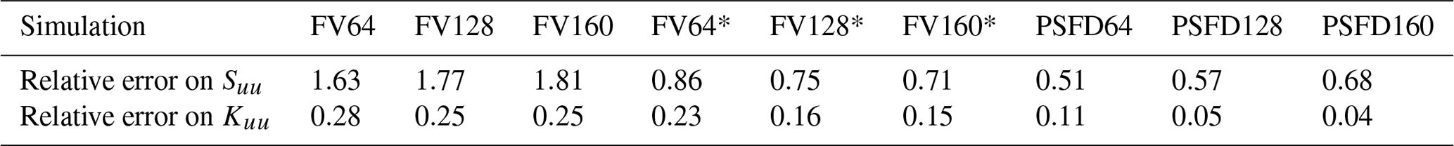
Skewness and kurtosis of the streamwise velocity (Suu and Kuu, respectively) are shown in Fig. 2. The profiles of Suu obtained with the FV-based solver and the QUICK scheme as well as those obtained with the PSFD-based solver are in good agreement with experimental results from Monty et al. (2009), here taken as a reference. On the contrary, the FV-based solver overpredicts Suu when the linear interpolation scheme is used, with the skewness remaining positive throughout the whole extent of the surface layer. Note that a positive skewness of streamwise velocity represents a flow field where negative fluctuations are more likely to happen than the corresponding positive ones. The kurtosis obtained with the FV-based solver is consistently overpredicted, representing a flow field populated by a greater number of extreme events. Again, profiles from all cases feature a nonmonotonic convergence to the reference ones, as shown in Table 3, where the relative error on skewness and kurtosis with respect to the measurements from Monty et al. (2009) is reported in the interval .
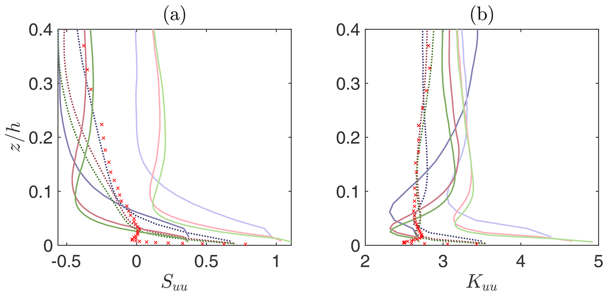
Figure 2Vertical structure of skewness of streamwise velocity (a) and kurtosis of streamwise velocity (b). Lines are defined in Fig. 1. The red x-marks denote the measurements from Monty et al. (2009), digitalized by the authors.
Table 3Relative error on skewness and kurtosis w.r.t. the measurements from Monty et al. (2009) in the interval .
3.2 Spectra and autocorrelations
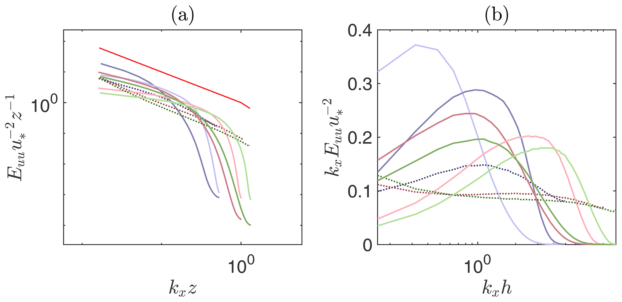
One-dimensional spectra of streamwise velocity fluctuations (Euu) are shown in Fig. 3a. The profiles are contrasted against the phenomenological production range and inertial subrange power-law profiles (k−1 and , respectively). Predictions from the PSFD-based solver feature a relatively good agreement with the phenomenological power-law profile, especially at high grid resolution. For example, the cases PSFD128 and PSFD160 exhibit a slope of −1.2 in the production range (here defined as kxz<1). Profiles from the FV-based solver, on the contrary, exhibit strong sensitivity to grid resolution and are unable to capture the expected power-law behavior. In the production range, velocity spectra from the FV solver start off relatively shallow at small wavenumber, especially when using the linear scheme. A narrow band can be identified where , followed by a rapid decay in energy density – the decay being particularly pronounced when using the QUICK interpolation scheme because of the associated numerical dissipation. Overall, the energy density in the production range and in the inertial subrange is not well captured by the FV-based solver and grid refinement does not help circumvent this limitation, at least at the considered resolutions. The authors note that this fact might limit the use of dynamic procedures based on the Germano et al. (1991) identity. A further characterization of the energy distribution in the wavenumber space is given in Fig. 3b, where premultiplied velocity spectra are shown. The usual reason for considering these quantities is to create a plot in semi-log scale where equal areas under the profiles correspond to equal energy. In addition, premultiplied spectra provide information on the coherence of the flow, in particular on the so-called large and very large scale motions (LSMs and VLSMs, respectively). These structures are responsible for carrying more than half of the kinetic energy and Reynolds shear stress and are a persistent feature of the surface and outer layers of both aerodynamically smooth and rough walls (Kim and Adrian, 1999; Balakumar and Adrian, 2007; Monty et al., 2007; Hutchins and Marusic, 2007; Fang and Porté-Agel, 2015). The current domain is of modest dimensions and is able to accommodate only LSMs (Lozano-Durán and Jiménez, 2014), which are identified in premultiplied spectra by a local maximum at the streamwise wavenumber . The location of the peaks from the FV-based solver with linear interpolation scheme shifts toward higher wavenumber with grid refinement, with a maximum at for the FV160 case. This fact signals a flow field where the streamwise extent of energetic modes (a.k.a., coherent structures) reduces as the grid is refined. On the contrary, the FV-based solver in combination with the QUICK scheme predicts the peak in premultiplied energy density at the expected wavenumber, hence suggesting that this approach is able to capture LSMs. The PSFD-based solver features a peak at the expected wavenumber (kx=1) only at the lowest resolution (PSFD64). Profiles from the higher-resolution cases feature high energy densities at the lowest wavenumber, highlighting an artificial “periodization” of energy-containing structures in the streamwise direction. This behavior is linked to the limited horizontal extent of the computational domain. The authors have indeed verified that a larger domain (twice as large along each horizontal direction) enables one to capture LSMs with the PSFD solver at resolutions matching the one of the PSFD128 case (not shown). A corresponding single run was carried out with the FV solver over the said larger domain and premultiplied spectra were found to be in good agreement with those presented herein, supporting the conjecture that the proposed domain size suffices to capture the range of variability of FV solvers for the problem under consideration.
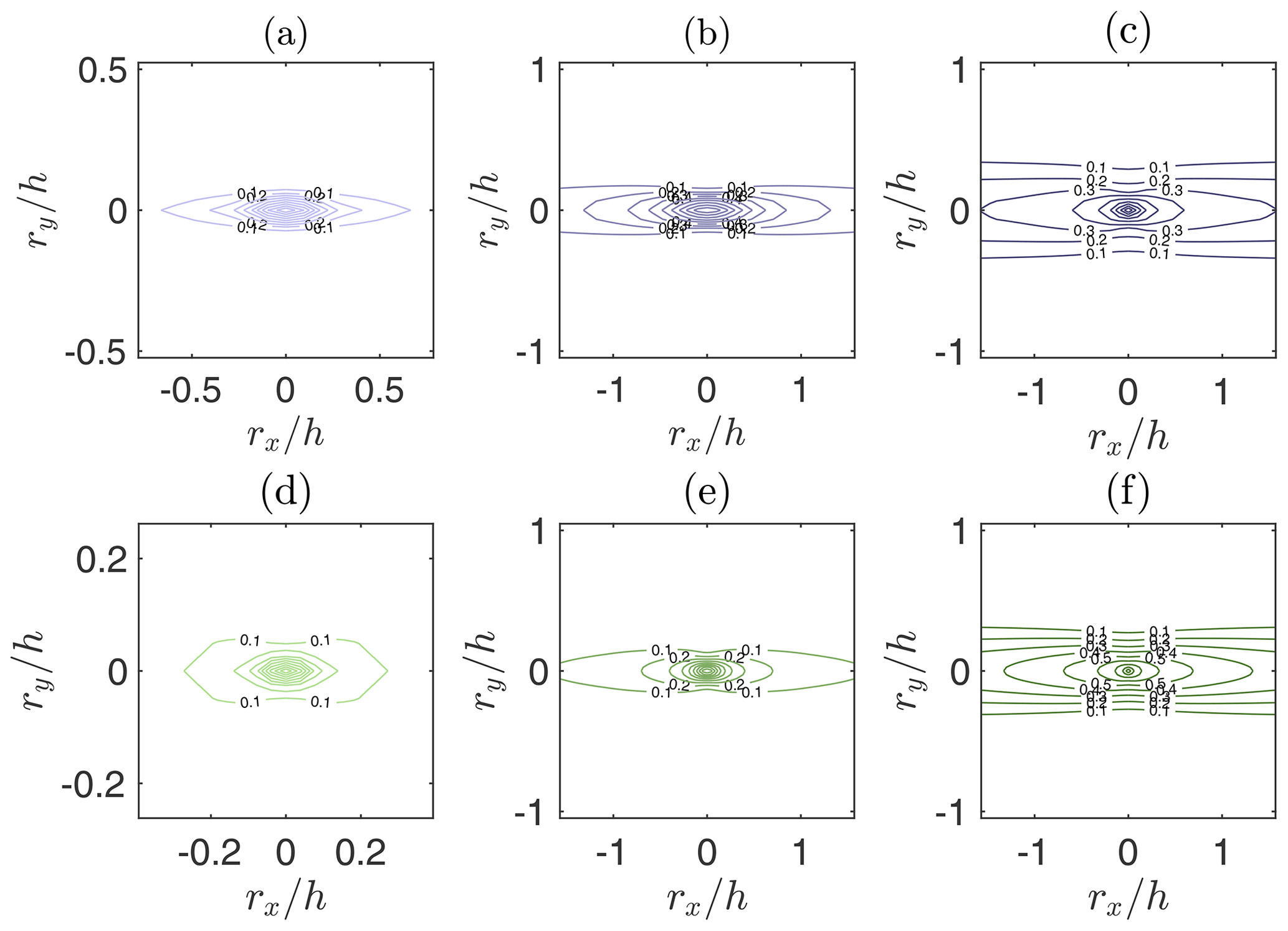
Figure 4Contours of two-dimensional spatial autocorrelation of streamwise velocity at height from the simulations FV64 (a), FV64* (b), PSFD64 (c), FV160 (d), FV160* (e), and PSFD160 (f). Contour levels from 0.1 to 0.9 with increments of 0.1.
To gain better insight on the spatial coherence of the flow field, the contour lines of the two-dimensional autocorrelation of the streamwise velocity in the xy plane are shown in Fig. 4. The contour is often used to identify the boundaries of coherent structures populating the flow field. The contours from the FV-based solver with linear scheme (Figs. 4a, d) are representative of a poorly correlated flow field with a streamwise extent of the contour of 0.5h and 0.1h along the streamwise and cross-stream directions, respectively. On the contrary, the contours from the FV-based solver with the QUICK scheme (Fig. 4b, e) depict a flow field characterized by larger spatial autocorrelation, in line with results from the PSFD-based solver. Note that the flow statistics presented above should not be impacted by the fact that the current domain size prevents some of the contour lines (simulations FV64*, FV160*, PSFD64, and PSFD160) from closing, as discussed in Lozano-Durán and Jiménez (2014).
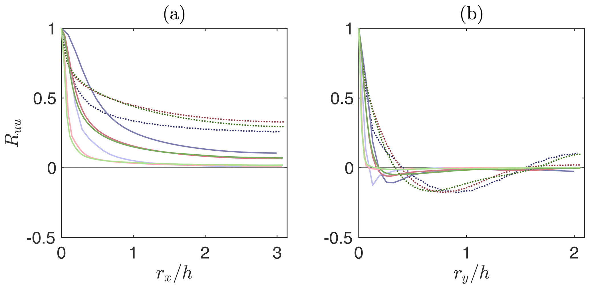
Figure 5One-dimensional spatial autocorrelation of streamwise velocity at height along the streamwise direction (a) and along the cross-stream direction (b). Lines as in Fig. 1.
The one-dimensional spatial autocorrelation (Ruu), shown in Fig. 5 along the streamwise and cross-stream directions, further corroborates the above findings. From Fig. 5a it is apparent that the extension of the selected domain does not enable the flow to become completely uncorrelated in the streamwise direction for the PSFD solver and for the FV solver using QUICK; Ruu remains finite in the available range across resolutions. On the other hand, profiles from the FV-based solver using the linear interpolation rapidly decay towards zero. Along the cross-stream direction (Fig. 5b), profiles from the PSFD-based solver feature the expected negative lobes, highlighting the presence of high- and low-momentum streamwise-elongated streaks flanking each other in the said direction. This behavior is in line with findings from previous studies on the coherence of wall-bounded turbulence and with standard turbulence theory. Profiles from the FV-based solver exhibit a similar profile, albeit featuring a more rapid decay and less prominent negative lobes, especially for the high-resolution cases using the linear interpolation scheme. A quantitative measure of the coherence of the flow field is provided in Table 4, where the integral lengths and are reported for all the considered cases and compared against direct numerical simulations of a channel flow at Reτ=2000 from Sillero et al. (2014). The integral lengths in Table 4 are evaluated at since the data from Sillero et al. (2014) are available at this height. Although might not be meaningful across the considered cases, owing to the lack of a zero crossing of the autocorrelation function, it is apparent that the FV-based solver underestimates the integral lengths when compared to the PSFD cases and the reference DNS values, especially when the linear interpolation scheme is used.
Sillero et al. (2014)
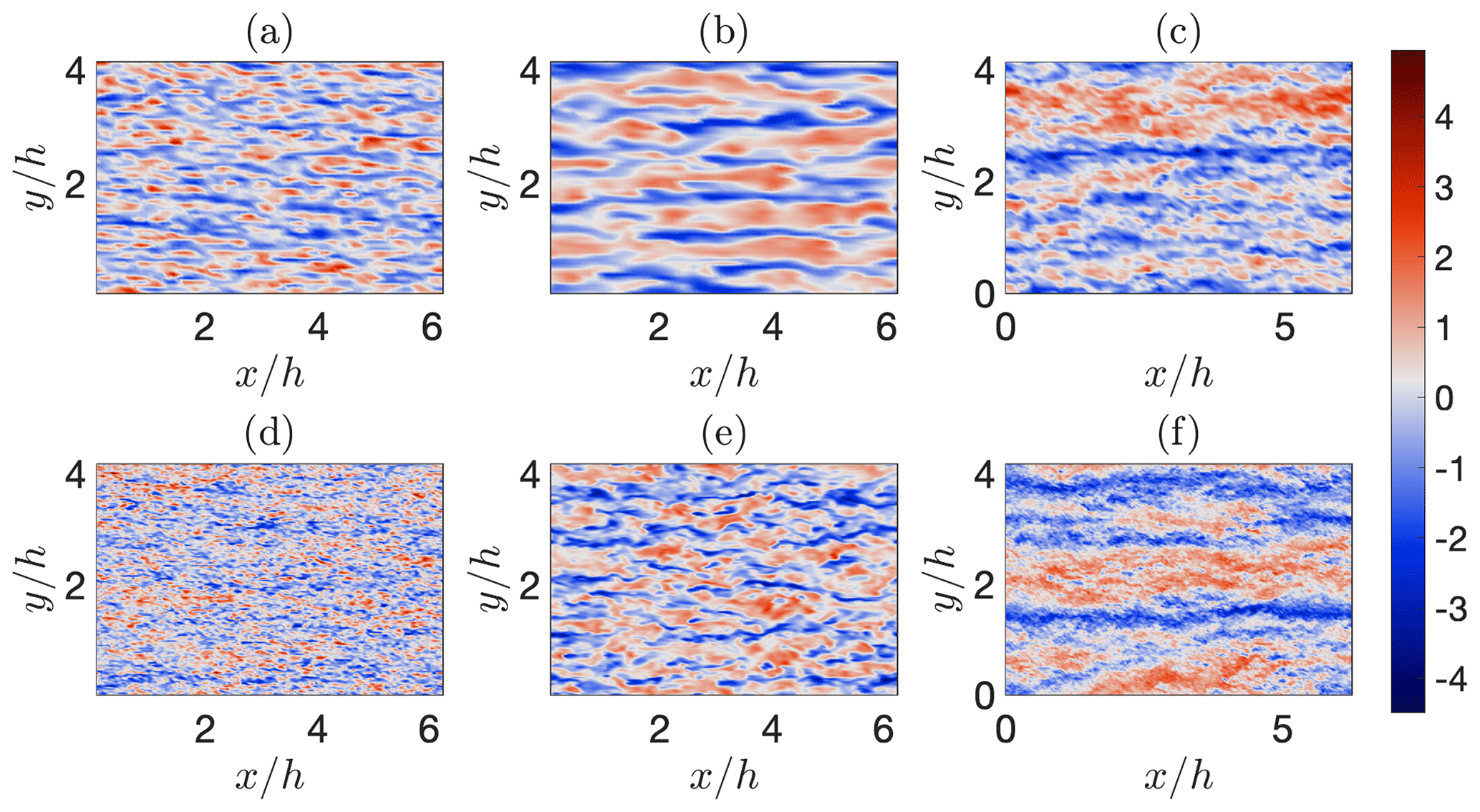
Figure 6Instantaneous snapshots of normalized streamwise velocity fluctuations at from the simulations FV64 (a), FV64* (b), PSFD64 (c), FV160 (d), FV160* (e), and PSFD160 (f). The normalized velocity fluctuation is defined as , where averages (and fluctuations therefrom) are evaluated in space over the selected horizontal plane.
Instantaneous snapshots of streamwise velocity fluctuations over a horizontal plane support the above findings (see Fig. 6). Artificially periodized, streamwise-elongated bulges of uniform high and low momentum are indeed apparent in the snapshots from the PSFD-based solver (Fig. 6c, f). On the contrary, the instantaneous streamwise velocity field from the FV solver is populated by smaller regions of uniform momentum, especially when using the linear scheme, and the size of energetic structures diminishes with increasing grid resolution (see, e.g., Fig. 6a, d).
3.3 Momentum transfer mechanisms
This section is devoted to the analysis of momentum transfer mechanisms in the ABL with a focus on quadrant analysis (Lu and Willmarth, 1973) and on statistics of conditionally averaged flow fields.
The quadrant hole analysis is a technique based on the decomposition of the velocity fluctuations into four quadrants: the first and third quadrants, outward interactions (, ) and inward interactions (, ), respectively, are negative contributions to the momentum flux, whereas the second and fourth quadrants, a.k.a. ejections of low-speed fluid outward from the wall (, ) and sweeps of high-speed fluid toward the wall (, ), represent positive contributions. A range of flow statistics can be defined based on this decomposition and used to provide insight on the mechanisms supporting momentum transfer in the ABL.

Figure 7Stress fractions at . The profiles are normalized so that the sum of the stress fractions for H=0 is unity across the cases. Lines are defined in Fig. 1.
Figure 7 features the quadrant-hole analysis, where the notation is the same as in Yue et al. (2007a), with H being the hole size, Si,H the resolved Reynolds shear stress contribution to the ith quadrant at hole size H, and is the corresponding quadrant fraction. Stress fractions are presented for values of the hole size H ranging from 0 to 8, where larger hole sizes correspond to contributions to the resolved Reynolds shear stress from more extreme events. Clearly, the FV-based solver with the linear scheme underpredicts ejections (Fig. 7a), outward interactions (Fig. 7b), and inward interactions (Fig. 7c), and overpredicts sweeps at large hole size H (Fig. 7d). On the contrary, the FV solver with the QUICK scheme underpredicts all the profiles except for the ejections, which are captured fairly well instead (see Fig. 7a). Note that ejections are violent events, concentrated over a very thin region in the cross-stream direction of the ABL (Fang and Porté-Agel, 2015).
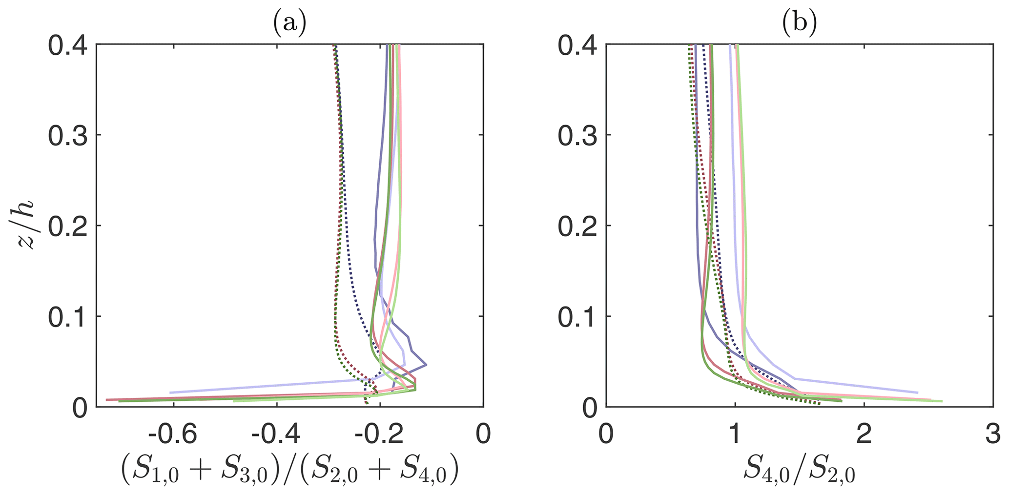
Figure 8Vertical structure of event ratios: (a) ratio of negative to positive contributions to the momentum flux; (b) ratio of sweeps to ejections. Lines as in Fig. 1.
To gain insight on the vertical structure of momentum transfer mechanisms, the exuberance ratio and the ratio of sweeps to ejections are analyzed in the following. Figure 8a shows the exuberance ratio, defined as the ratio of negative to positive contributions to the momentum flux, (Shaw et al., 1983). The exuberance ratios from the PSFD-based solver are larger in absolute value than the correspondent ones from the FV-based solver across the whole surface layer except very close to the surface. Profiles highlight that outward and inward interactions have a significant impact on the resolved Reynolds stress in the PSFD-based solver, whereas the flow simulated with the FV-based solver is characterized by a predominance of sweeps and ejections. This behavior is consistent throughout the ABL. Figure 8b shows the ratio of sweeps to ejections at the lowest portion of the ABL (). Profiles obtained with the QUICK scheme are in line with predictions from the PSFD-based solver and with findings from measurements of surface-layer flow over rough surfaces, where ejections are identified as the dominant momentum transport mechanism in the ABL (Raupach et al., 1991). On the contrary, the FV-based solver with a linear scheme tends to favor sweeps over ejections as the mechanisms for momentum transfer in the surface layer.
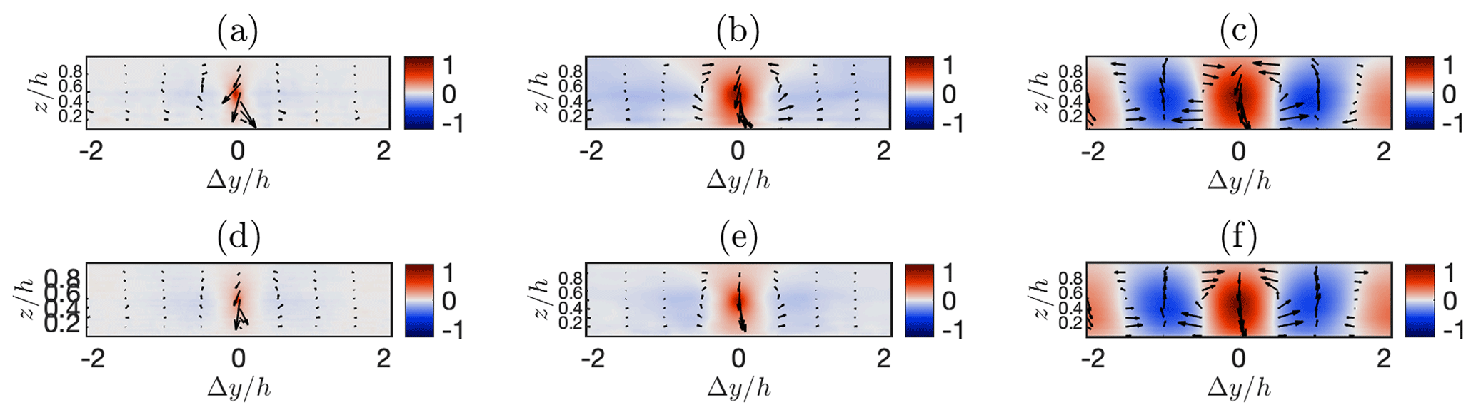
Figure 9Visualization of the conditionally averaged velocity field in the cross-stream vertical plane at from simulations FV64 (a), FV64* (b), PSFD64 (c), FV160 (d), FV160* (e), and PSFD160 (f). The conditional event is a positive streamwise velocity fluctuation at , , and . Colors are used to represent the magnitude of the streamwise component and vectors denote the cross-stream and vertical components.
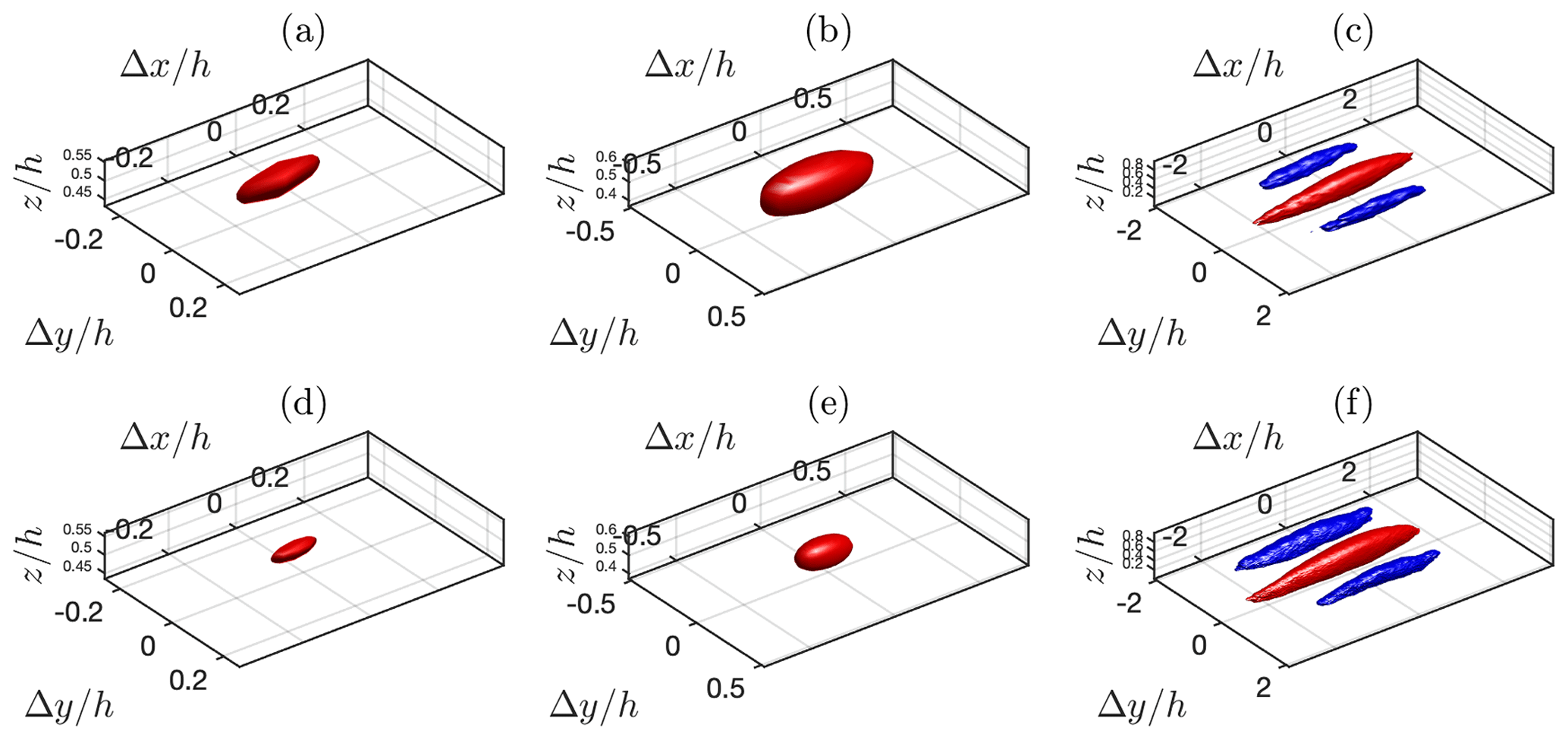
Figure 10Conditionally averaged flow field from simulations FV64 (a), FV64* (b), PSFD64 (c), FV160 (d), FV160* (e), and PSFD160 (f). The conditional average is computed as in Fig. 9. Red isosurfaces show positive fluctuations (>0.7, top; >0.65, bottom); blue isosurfaces show negative fluctuations (, top; , bottom).
To conclude the analysis on the mechanisms responsible for momentum transfer, velocity statistics from a conditionally averaged flow field are discussed next. The approach of Fang and Porté-Agel (2015) is adopted to compute the conditionally averaged flow field, where the conditional event is a positive streamwise velocity fluctuation at , , and . Figure 9 features a pseudocolor and vector plot of the conditionally averaged velocity field in a cross-stream vertical plane for selected cases, whereas Fig. 10 displays a three-dimensional isosurface thereof. The flow structure in the equilibrium surface layer is known to be characterized by counter-rotating rolls and low- and high-momentum streamwise-elongated streaks flanking each other in the cross-stream direction. Rolls and streaks are indeed the dominant flow mechanism responsible for tangential Reynolds stress (Ganapatisubramani et al., 2003; Lozano-Durán et al., 2012). As apparent from Fig. 9, the PSFD conditionally averaged velocity field exhibits counter-rotating patterns associated with positive and negative streamwise velocity fluctuations (corresponding to the aforementioned streaks). Throughout the ABL, the roll modes feature a diameter that is consistent with findings from the literature (d≈h). Moreover, positive and negative velocity fluctuations are approximately of the same magnitude . From Fig. 10, it is apparent that the considered isosurfaces extend about 4h along the streamwise direction. Quite surprisingly, the FV-based solver is not able to predict the roll modes, irrespective of the interpolation scheme and grid resolution, and severely underpredicts the magnitude of the low-momentum streaks. Further, Figs. 9 and 10 both depict a FV conditionally averaged flow field that is poorly correlated along the cross-stream and streamwise directions, resulting in significantly smaller momentum-carrying structures. This fact supports previous findings from the two-dimensional spatial autocorrelation (Fig. 4). The lack of roll modes implies that the FV-based solvers used here are not able to capture the fundamental mechanism supporting momentum transfer in the ABL, at least at the considered grid resolutions. This limitation is likely to be the root cause of several of the observed problematics associated with the FV-solver solution, including the relatively high (low) streamwise-velocity skewness when using linear (QUICK) schemes (see Fig. 2,a) and the observed imbalance between sweeps and ejections (Figs. 1 and 8).
The present work provides insight on the quality and reliability of an important class of general-purpose, second-order accurate FV-based solvers for the wall-modeled LES of neutrally stratified ABL flow. The considered FV-based solvers are part of the OpenFOAM® framework, make use of the divergence form for the nonlinear term, and are based on a colocated grid arrangement.
A suite of simulations was carried out in an open-channel flow setup, varying the grid resolution up to 1603 control volumes, the interpolation schemes for the discretization of the nonlinear term, the value of the Smagorinsky coefficient, the pressure-velocity coupling method, and the time-advancement scheme. Several flow statistics were contrasted against profiles from a well-established PSFD-based solver and against experimental measurements when these were available. Considered flow statistics include mean velocity, turbulence intensities, velocity skewness and kurtosis, velocity spectra, and spatial autocorrelations. An analysis of mechanisms supporting momentum transfer in the flow field was also proposed. The main findings are summarized below.
With the exception of the FV solver with the projection method and the Runge–Kutta time-advancement scheme, mean velocity profiles from the PSFD and FV solvers all feature a positive LLM. Existing techniques to alleviate this limitation led to no apparent improvement, thus calling for alternative approaches.
Near-surface streamwise velocity fluctuations are consistently overpredicted by both the PSFD and FV solvers, irrespective of the grid resolution. The overshoot is particularly pronounced for the cases based on the QUICK interpolation scheme. This behavior can be related to a deficit of pressure redistribution in the budget equations for the velocity variances, which results in a pile-up of shear-generated streamwise velocity fluctuations and deficit in the vertical and cross-stream velocity fluctuation components.
The interpolation scheme used for the discretization of the nonlinear term plays a role in determining the remaining flow statistics. Specifically, FV solvers with a linear interpolation scheme lead to
-
a positive streamwise velocity skewness throughout the surface layer, which is at odds with experimental findings;
-
a severe overprediction of the streamwise velocity kurtosis;
-
a poorly correlated streamwise velocity field in the horizontal directions, especially at high grid resolutions;
-
a severe underprediction of outward and inward interactions and ejection events;
-
a lack of organized high- and low-momentum streaks and associated roll modes in the conditionally averaged flow field.
Grid resolution either does not affect the above quantities or leads to larger departures from the expected behavior. The QUICK scheme, on the other hand, leads to
-
an improved prediction of the streamwise velocity skewness and kurtosis, especially as the grid stencil is reduced;
-
a streamwise velocity field that is more correlated along the horizontal directions, but integral length scales remain only a fraction of those from the PSFD and reference DNS results;
-
an underprediction of inward and outward interactions;
-
a lack of organized high- and low-momentum streaks and associated roll modes in the conditionally averaged flow field.
To summarize, the considered class of FV-based solvers predicts a flow field that is less correlated than the one obtained with the PSFD solver and does not capture the salient mechanisms responsible for momentum transfer in the ABL, at least at the considered grid resolutions. These limitations appear to be the root cause of many of the observed discrepancies between FV flow statistics and the corresponding PSFD or experimental ones, including the mispredicted streamwise-velocity skewness (Fig. 2a), the imbalance between sweeps and ejections (Figs. 1 and 8), and the overall sensitivity of flow statistics to variations in the grid resolution. Higher grid resolutions might help alleviate some of these shortcomings, but given that grid resolutions used herein are state-of-the-art for general-purpose FV-based solvers and that computing power increases relatively slowly with time (Moore, 1965), the aforementioned limitations are likely to persist for years to come, thus introducing a degree of uncertainty in model results that needs to be addressed. These limitations call for research aimed at reducing the impact of discretization errors in this class of solvers, or for alternative approaches such as using discretizations based on staggered grid arrangements and higher-order spatial discretization schemes.
A1 Smagorinsky constant
We here test the sensitivity of selected flow statistics to variations in the Smagorinsky constant CS. The values CS=0.1, CS=0.12, CS=0.14, CS=0.16, and CS=0.1678 (the default value in OpenFOAM®) are considered, and all tests are carried out at 643 control volumes.
As shown in Fig. A1a, the Smagorinsky constant has a relatively important and nonmonotonic impact on the mean velocity profile. The case at CS=0.1 results in the largest positive LLM, in agreement with the predictions from the PSFD-based solver, whereas the cases at larger CS exhibit a smaller, albeit still positive, LLM. The Smagorinsky coefficient also has a discernible impact on the velocity RMSs. Specifically, as CS is increased, the magnitude of the near-surface maximum for both (Fig. A1b) and (Fig. A1c) is reduced, and the location of the maximum is shifted away from the surface – possibly the result of a higher near-surface energy dissipation. In addition, larger values of CS yield a more apparent departure from the corresponding profiles obtained with the PSFD-based solver.
The one-dimensional spectra (Fig. A2a) show that larger values of the Smagorinsky coefficient result in a more rapid decay of energy density and in a shift of profiles toward the inertial subrange. No value of the Smagorinsky coefficient seems suitable for capturing the k−1 power law in the production range of turbulence. Increasing CS leads to a modest improvement in the two-point autocorrelation profiles (Fig. A2b, c).
A2 Solvers
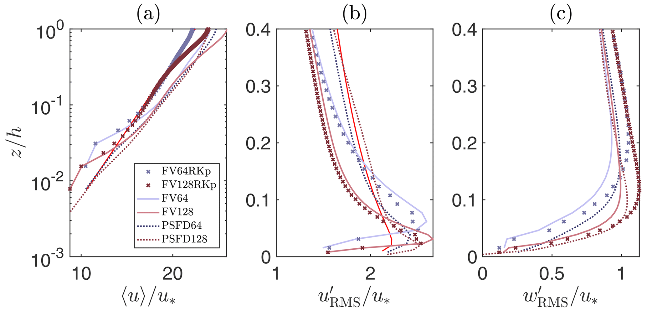
The performance of an alternative solver within the OpenFOAM® framework is considered here, and the results are contrasted against those previously shown (obtained with the PISO algorithm in combination with an Adams–Moulton time-advancement scheme). The solver is based on a projection method coupled with the Runge–Kutta 4 time-advancement scheme (Ferziger and Peric, 2002). Details on the implementation can be found in Vuorinen et al. (2015). The performances of the two solvers are compared at moderate Reynolds number in Vuorinen et al. (2014), where it is pointed out that the projection method coupled with the Runge–Kutta 4 time-advancement scheme provides similar results at lower computational cost. In the following, the performances of the solver are tested for the considered ABL flow. Two grid resolutions are considered based on 643 (case FV64RKp) and 1283 (case FV128RKp) control volumes.
The vertical profile of the mean streamwise velocity is shown in Fig. A3a. The use of the projection Runge–Kutta 4 solver leads to an underprediction of the velocity at the wall as for the simulations FV64 and FV128, but no apparent LLM in the surface layer. exhibits the previously observed near-surface peaks (Fig. A3b) whereas is overpredicted above (Fig. A3c).
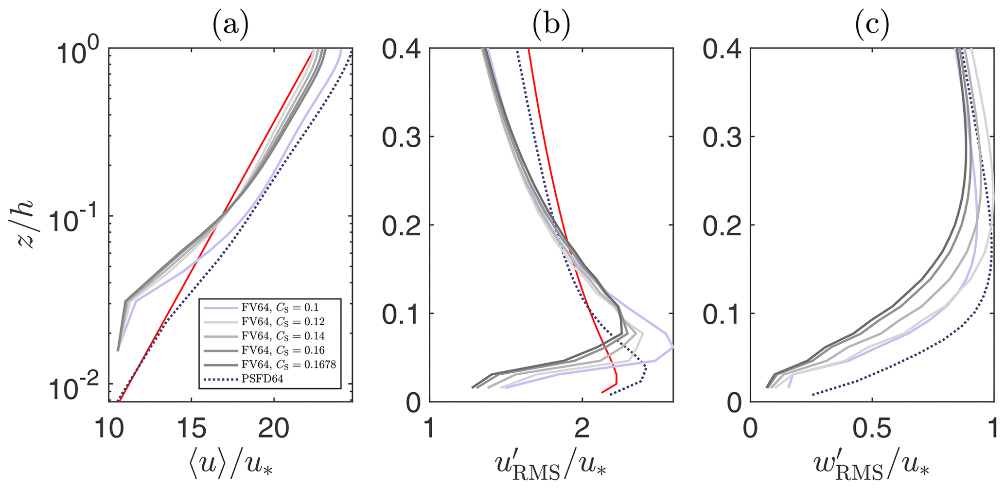
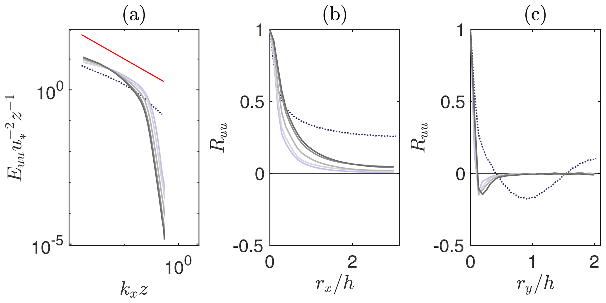
Figure A2Normalized one-dimensional spectra of streamwise velocity at (a); one-dimensional spatial autocorrelation of streamwise velocity at along the streamwise direction (b) and along the cross-stream direction (c). Lines as in Fig. A1. The red line denotes (kxz)−1.
OpenFOAM® is an open-source computational fluid dynamics toolbox. The present study made use of OpenFOAM® version 6.0, available for download at https://openfoam.org/version/6/ (last access: 3 March 2021.
Data and script to generate all figures in this manuscript can be downloaded from: https://doi.org/10.7916/d8-199p-bk19 (Giacomini and Giometto, 2021).
BG and MGG designed the study. BG conducted the analysis under the supervision of MGG. BG and MGG wrote the manuscript.
The authors declare that they have no conflict of interest.
The authors acknowledge computing resources from Columbia University's Shared Research Computing Facility project, which is supported by NIH Research Facility Improvement Grant 1G20RR030893-01, and associated funds from the New York State Empire State Development, Division of Science Technology and Innovation (NYSTAR) Contract C090171, both awarded 15 April 2010. The authors are grateful to Weiyi Li for generating the PSFD data, and to Ville Vuorinen and George I. Park for useful discussions on the performance of FV-based solvers for the simulation of turbulent flows.
The work was supported via start-up funds provided by the Department of Civil Engineering and Engineering Mechanics at Columbia University.
This paper was edited by Chiel van Heerwaarden and reviewed by two anonymous referees.
Abkar, M. and Porté-Agel, F.: The effect of free-atmosphere stratification on boundary-layer flow and power output from very large wind farms, Energies, 6, 2338–2361, 2013. a
Albertson, J. D. and Parlange, M. B.: Natural integration of scalar fluxes from complex terrain, Adv. Water Resour., 23, 239–252, 1999. a, b
Anderson, W. and Meneveau, C.: A large-eddy simulation model for boundary-layer flow over surfaces with horizontally resolved but vertically unresolved roughness elements, Bound.-Lay. Meteorol., 137, 397–415, 2010. a
Bae, H. J., Lozano-Durán, A., Bose, S. T., and Moin, P.: Turbulence intensities in large-eddy simulation of wall-bounded flows, Phys. Rev. Fluids, 3, 014610, https://doi.org/10.1103/PhysRevFluids.3.014610, 2018. a
Bailey, B. N. and Stoll, R.: Turbulence in sparse, organized vegetative canopies: A large-eddy simulation study, Bound.-Lay. Meteorol., 147, 369–400, 2013. a
Balakumar, B. J. and Adrian, R. J.: Large- and very-large-scale motions in channel and boundary-layer flows, Philos. T. Roy. Soc. A, 365, 665–681, 2007. a
Balogh, M., Parente, A., and Benocci, C.: RANS simulation of ABL flow over complex terrains applying an enhanced k-ϵ model and wall function formulation: implementation and comparison for fluent and OpenFOAM, J. Wind Eng. Ind. Aerodyn., 104–106, 360–368, 2012. a
Beaudan, P. and Moin, P.: Numerical experiments on the flow past a circular cylinder at sub-critical Reynolds number, Tech. rep., Thermosciences Div., Stanford University, California, 1994. a
Bose, S. T. and Moin, P.: A dynamic slip boundary condition for wall-modeled large-eddy simulation, Phys. Fluids, 26, 015104, 2014. a
Bose, S. T. and Park, G. I.: Wall-modeled large-eddy simulation for complex turbulent flows, Annu. Rev. Fluid Mech., 50, 535–561, 2018. a
Bou-Zeid, E., Meneveau, C., and Parlange, M. B.: A scale-dependent Lagrangian dynamic model for large eddy simulation of complex turbulent flows, Phys. Fluids, 17, 025105, https://doi.org/10.1063/1.1839152, 2005. a, b, c
Bou-Zeid, E., Overney, J., Rogers, B. D., and Parlange, M. B.: The effects of building representation and clustering in large-eddy simulations of flows in urban canopies, Bound.-Lay. Meteorol., 132, 415–436, 2009. a
Breuer, M.: Large eddy simulation of the subcritical flow past a circular cylinder: Numerical and modeling aspects, Int. J. Numer. Meth. Fluids, 28, 1281–1302, 1998. a
Calaf, M., Meneveau, C., and Meyers, J.: Large eddy simulation study of fully developed wind-turbine array boundary layers, Phys. Fluids, 22, 015110, 2010. a, b
Chester, S., Meneveau, C., and Parlange, M. B.: Modeling turbulent flow over fractal trees with renormalized numerical simulation, J. Comput. Phys., 225, 427–448, 2007. a
Chow, F., Street, R., Xue, M., and Ferziger, J.: Explicit filtering and reconstruction turbulence modeling for large-eddy simulation of neutral boundary layer flow, J. Atmos. Sci., 62, 2058–2076, 2005. a
Churchfield, M., Vijayakumar, G., Brasseur, J., and Moriarty, P.: Wind energy-related atmospheric boundary layer large-eddy simulation using OpenFOAM, presented as Paper 1B.6 at the American Meteorological Society, 19th Symposium on Boundary Layers and Turbulence NREL/CP-500-48905, National Renewable Energy Laboratory, Colorado, 2010. a, b
Churchfield, M., Lee, S., and Moriarty, P.: Adding complex terrain and stable atmospheric condition capability to the OpenFOAM-based flow solver of the simulator for on/offshore wind farm applications (SOWFA), presented at the 1st symposium on OpenFOAM in Wind Energy, Oldenburg, Germany, National Renewable Energy Laboratory, 2013. a
De Villiers, E.: The potential for large eddy simulation for the modeling of wall bounded flows, PhD thesis, Imperial College of Science, Technology and Medicine, London, 2006. a
Deardorff, J. W.: A numerical study of three-dimensional turbulent channel flow at large Reynolds numbers, J. Fluid Mech., 41, 453–480, 1970. a
Fang, J. and Porté-Agel, F.: Large-eddy simulation of very-large-scale motions in the neutrally stratified atmospheric boundary layer, Bound.-Lay. Meteorol., 155, 397–416, 2015. a, b, c
Fang, J., Diebold, M., Higgins, C., and Parlange, M. B.: Towards oscillation-free implementation of the immersed boundary method with spectral-like methods, J. Comput. Phys., 230, 8179–8191, 2011. a
Fernando, H. J. S.: Fluid dynamics of urban atmospheres in complex terrain, Annu. Rev. Fluid Mech., 42, 365–389, 2010. a
Ferziger, J. and Peric, M.: Computational methods for fluid dynamics, Springer, 2002. a, b, c, d, e, f
Ganapatisubramani, B., Longmire, E. K., and Marusic, I.: Characteristics of vortex packets in turbulent boundary layers, J. Fluid Mech., 478, 35–46, 2003. a
García-Sánchez, C. and Gorlé, C.: Uncertainty quantification for microscale CFD simulations based on input from mesoscale codes, J. Wind Eng. Ind. Aerod., 176, 87–97, 2018. a
García-Sánchez, C., Tendeloo, G. V., and Gorlé, C.: Quantifying inflow uncertainties in RANS simulations of urban pollutant dispersion, Atmos. Environ., 161, 263–273, 2017. a
Germano, M., Piomelli, U., Moin, P., and Cabot, W.: A dynamic subgrid-scale eddy viscosity model, Phys. Fluids, 3, 1760–1765, 1991. a, b, c, d
Ghosal, S.: An Analysis of Numerical Errors in Large-Eddy Simulations of Turbulence, J. Comput. Phys., 125, 187–206, 1996. a
Giacomini, B. and Giometto, M. G.: On the suitability of second-order accurate finite-volume solvers for the simulation of atmospheric boundary layer flow, Columbia University Libraries, https://doi.org/10.7916/d8-199p-bk19, 2021. a
Giometto, M., Katul, G., Fang, J., and Parlange, M. B.: Direct numerical simulation of turbulent slope Flows up to Grashof number Gr=2^11, J. Fluid Mech., 829, 589–620, 2017. a
Hultmark, M., Calaf, M., and Parlange, M. B.: A new wall shear stress model for atmospheric boundary layer simulations, J. Atmos. Sci., 70, 3460–3470, 2013. a, b, c, d
Hutchins, N. and Marusic, I.: Evidence of very long meandering features in the logarithmic region of turbulent boundary layers, J. Fluid Mech., 579, 1–28, 2007. a
Issa, R.: Solution of the implicitly discretised fluid flow equations by operator-splitting, J. Comput. Phys., 62, 40–65, 1985. a
Jasak, H., Jemcov, A., and Tukovic, Z.: OpenFOAM: A C++ library for complex physics simulations, Presented at the International Workshop on Coupled Methods in Numerical Dynamics, IUC, Dubrovnik, Croatia, 2007. a
Kawai, S. and Larsson, J.: Wall-modeling in large eddy simulation: Length scales, grid resolution, and accuracy, Phys. Fluids, 24, 015105, https://doi.org/10.1063/1.3678331, 2012. a, b, c
Kim, K. C. and Adrian, R. J.: Very large-scale motion in the outer layer, Phys. Fluids, 11, 417–422, 1999. a
Kravchenko, A. and Moin, P.: On the effect of numerical errors in large eddy simulations of turbulent flows, J. Comput. Phys., 131, 310–322, 1997. a, b, c
Li, Q. and Bou-Zeid, E.: Contrasts between momentum and scalar transport over very rough surfaces, J. Fluid Mech., 880, 32–58, 2019. a
Li, Q., Bou-Zeid, E., and Anderson, W.: The impact and treatment of the Gibbs phenomenon in immersed boundary method simulations of momentum and scalar transport, J. Comput. Phys., 310, 237–251, 2016. a
Lilly, D. K.: A proposed modification of the Germano subgridscale closure method, Phys. Fluids, 4, 633–635, 1992. a, b
Lozano-Durán, A. and Jiménez, J.: Effects of the computational domain on direct simulations of turbulent channels up to Reτ=4200, Phys. Fluids, 26, 011702, 2014. a, b
Lozano-Durán, A., Flores, O., and Jiménez, J.: The three-dimensional structure of momentum transfer in turbulent channels, J. Fluid Mech., 649, 100–130, 2012. a
Lu, S. and Willmarth, W.: Measurements of the structure of the Reynolds stress in a turbulent boundary layer, J. Fluid Mech., 60, 481–511, 1973. a
Majander, P. and Siikonen, T.: Evaluation of Smagorinsky-based subgrid-scale models in a finite-volume computation, Int. J. Numer. Meth. Fluids, 40, 735–774, 2002. a
Margairaz, F., Giometto, M. G., Parlange, M. B., and Calaf, M.: Comparison of dealiasing schemes in large-eddy simulation of neutrally stratified atmospheric flows, Geosci. Model Dev., 11, 4069–4084, https://doi.org/10.5194/gmd-11-4069-2018, 2018. a
Maronga, B., Gryschka, M., Heinze, R., Hoffmann, F., Kanani-Sühring, F., Keck, M., Ketelsen, K., Letzel, M. O., Sühring, M., and Raasch, S.: The Parallelized Large-Eddy Simulation Model (PALM) version 4.0 for atmospheric and oceanic flows: model formulation, recent developments, and future perspectives, Geosci. Model Dev., 8, 2515–2551, https://doi.org/10.5194/gmd-8-2515-2015, 2015. a
Meneveau, C. and Lund, T. S.: The dynamic Smagorinsky model and scale-dependent coefficients in the viscous range of turbulence, Phys. Fluids, 9, 3932, https://doi.org/10.1063/1.869493, 1997. a
Meyers, J. and Sagaut, P.: Is plane-channel flow a friendly case for the testing of large-eddy simulation subgrid-scale models?, Phys. Fluids, 19, 048105, https://doi.org/10.1063/1.2722422, 2007. a, b
Meyers, J., Sagaut, P., and Geurts, B. J.: Optimal model parameters for multi-objective large-eddy simulations, Phys. Fluids, 18, 095103, 2006. a, b
Meyers, J., Geurts, B. J., and Sagaut, P.: A computational error-assessment of central finite-volume discretizations in large-eddy simulation using a Smagorinsky model, J. Comput. Phys., 227, 156–173, 2007. a, b, c
Mittal, R. and Moin, P.: Suitability of upwind-biased finite difference schemes for large-Eddy simulation of turbulent flows, AIAA Journal, 35, 1415–1417, 1997. a
Moeng, C.: A large-eddy-simulation model for the study of planetary boundary-layer turbulence, J. Atmos. Sci., 41, 2052–2062, 1984. a
Moin, P., Reynolds, W., and Ferziger, J.: Large eddy simulation of incompressible turbulent channel flow, Tech. Rep. TF-12, Thermosciences Div., Stanford University, California, 1978. a
Momen, M., Bou-Zeid, E., Parlange, M. B., and Giometto, M. G.: Modulation of mean wind and turbulence in the atmospheric boundary layer by baroclinicity, J. Atmos. Sci., 76, 3797–3821, 2018. a
Montecchia, M., Brethouwer, G., Wallin, S., Johansson, A. V., and Knacke, T.: Improving LES with OpenFOAM by minimising numerical dissipation and use of explicit algebraic SGS stress model, J. Turbulence, 20, 697–722, 2019. a
Monty, J., Hutchins, N., NG, H., Marusic, I., and Chong, M.: A comparison of turbulent pipe, channel and boundary layer flows, J. Fluid Mech., 632, 431–442, 2009. a, b, c, d
Monty, J. P., Steward, J. A., Williams, R. C., and Chong, M. S.: Large-scale features in turbulent pipe and channel flows, J. Fluid Mech., 589, 147–156, 2007. a
Moore, G. E.: Cramming more components onto integrated circuits, Proc. IEEE, 86, 82–85, 1965. a
Mukha, T., Rezaeiravesh, S., and Liefvendahl, M.: A library for wall-modelled large-eddy simulation based on OpenFOAM technology, Comput. Phys. Commun., 239, 204–224, 2019. a
Oke, T. R., Mills, G., Christen, A., and Voogt, J. A.: Urban Climates, Cambridge University Press, Cambridge, https://doi.org/10.1017/9781139016476, 2017. a
Orlandi, P.: Fluid flow phenomena: A numerical toolkit, vol. 55, Springer Science & Business Media, Kluwer Academic Publishers, Dordrecht, the Netherlands, 2000. a
Pan, Y., Follett, E., Chamecki, M., and Nepf, H.: Strong and weak, unsteady reconfiguration and its impact on turbulence structure within plant canopies, Phys. Fluids, 26, 105102, https://doi.org/10.1063/1.4898395, 2014. a
Piomelli, U.: Wall-layer models for large-eddy simulations, Prog. Aerospace Sci., 44, 437–446, 2008. a
Porté-Agel, F.: A scale-dependent dynamic model for scalar transport in large-eddy simulations of the atmospheric boundary layer, Bound.-Lay. Meteorol., 112, 81–105, 2004. a
Porté-Agel, F., Meneveau, C., and Parlange, M. B.: A scale-dependent dynamic model for large-eddy simulation: application to a neutral atmospheric boundary layer, J. Fluid Mech., 415, 261–284, 2000. a
Powers, J. G., Klemp, J. B., Skamarock, W. C., Davis, C. A., Dudhia, J., Gill, D. O., Coen, J. L., Gochis, D. J., Ahmadov, R., Peckham, S. E., Grell, G. A., Michalakes, J., Trahan, S., Benjamin, S. G., Alexander, C. R., Dimego, G. J., Wang, W., Schwartz, C. S., Romine, G. S., Liu, Z., Snyder, C., Chen, F., Barlage, M. J., Yu, W., and Duda, M. G.: The weather research and forecasting model: Overview, system efforts, and future directions, B. Am. Meteorol. Soc., 98, 1717–1737, 2017. a
Raasch, S. and Schröter, M.: PALM – A large-eddy simulation model performing on massively parallel computers, Meteorol. Z., 10, 363–372, 2001. a
Raupach, M., Antonia, R., and Rajagopalan, S.: Rough-wall turbulent boundary layers, Appl. Mech. Rev., 44, 1–25, 1991. a
Rezaeiravesh, S. and Liefvendahl, M.: Effect of grid resolution on large eddy simulation of wall-bounded turbulence, Phys. Fluids, 30, 055106, 2018. a
Rhie, C. and Chow, W.: Numerical study of the turbulent flow past an airfoil with trailing edge separation, AIAA J., 21, 1525–1532, 1983. a
Salesky, S., Chamecki, M., and Bou-Zeid, E.: On the nature of the transition between roll and cellular organization in the convective boundary layer, Bound.-Lay. Meteorol., 163, 41–68, 2017. a, b
Scotti, A., Meneveau, C., and Lilly, D. K.: Generalized Smagorinsky model for anisotropic grids, Phys. Fluids A, 5, 2306–2308, 1993. a
Shaw, R., Tavangar, J., and Ward, D.: Structure of the Reynolds stress in canopy layer, J. Climate Appl. Meteorol., 22, 1922–1931, 1983. a
Shaw, W. J., Draxl, C., Mirocha, J., Muradyan, P., Ghate, V., Optis, M., and Lemke, A.: Workshop on Research Needs for Offshore Wind Resource Characterization, Tech. rep., U.S. Department of Energy, Alexandria, VA, 2019. a
Shi, L. and Yeo, D.: OpenFOAM large-eddy simulations of atmospheric boundary layer turbulence for wind engineering applications, Tech. rep., National Institute of Standards and Technology, Gaithersburg, Maryland, 2016. a
Shi, L. and Yeo, D.: Large eddy simulations of model-scale turbulent atmospheric boundary layer flows, J. Eng. Mech., 143, 06017011, 2017. a
Sillero, J. A., Jiménez, J., and Moser, R. D.: Two-point statistics for turbulent boundary layers and channels at Reynolds numbers up to , Phys. Fluids, 26, 105109, https://doi.org/10.1063/1.4899259, 2014. a, b, c
Skamarock, W. C. and Klemp, J. B.: A time-split nonhydrostatic atmospheric model for weather research and forecasting applications, J. Comput. Phys., 227, 3465–3485, 2008. a
Smagorinsky, J.: General circulation experiments with the primitive equations, Mon. Weather Rev., 91, 99–164, 1963. a
Stevens, R. and Meneveau, C.: Flow structure and turbulence in wind farms, Annu. Rev. Fluid Mech., 49, 311–339, 2017. a
Stovall, T., Pawlas, G., and Moriarty, P.: Wind farm wake simulations in OpenFOAM, presented at the 48th AIAA Aerospace Sciences Meeting Including the New Horizons Forum and Aerospace Exposition AIAA 2010-825, American Institute of Aeronautics and Astronautics, 4–7 January 2010, Orlando, Florida, 2010. a
Stull, R. B.: An introduction to boundary layer meteorology, Springer Netherlands, Dordrecht, 1988. a, b
Sullivan, P., McWilliams, J., and Moeng, C.-H.: A subgrid-scale model for large-eddy simulation of planetary boundary-layer flows, Bound.-Lay. Meteorol., 71, 247–276, 1994. a
Tseng, Y. H., Meneveau, C., and Parlange, M. B.: Modeling flow around bluff bodies and predicting urban dispersion using large eddy simulation, Environ. Sci. Technol., 40, 2653–2662, 2006. a
Vuorinen, V., Keskinen, J. P., Duwig, C., and Boersma, B. J.: On the implementation of low-dissipative Runge-Kutta projection methods for time dependent flows using OpenFOAM®, Comput. Fluids, 93, 153–163, 2014. a, b, c
Vuorinen, V., Chaudhari, A., and Keskinen, J.-P.: Large-eddy simulation in a complex hill terrain enabled by a compact fractional step OpenFOAM® solver, Adv. Eng. Softw., 79, 70–80, 2015. a
Weller, H. G., Tabor, G., Jasak, H., and Fureby, C.: A tensorial approach to computational continuum mechanics using object-oriented techniques, Comput. Phys., 12, 620, https://doi.org/10.1063/1.168744, 1998. a
Whiteman, C.: Mountain meteorology: fundamentals and applications, Oxford University Press, New York, 2000. a
Wu, P. and Meyers, J.: A constraint for the subgrid-scale stresses in the logarithmic region of high Reynolds number turbulent boundary layers: a solution to the log-layer mismatch problem, Phys. Fluids, 25, 015104, https://doi.org/10.1063/1.4774344, 2013. a
Xiang, I., Park, G., and Moin, P.: Log-layer mismatch and modeling of the fluctuating wall stress in wall-modeled large-eddy simulations, Phys. Rev. Fluids, 2, 104601, 2017. a
Yue, W., Meneveau, C., Parlange, M., Zhu, W., Van Hout, R., and Katz, J.: A comparative quadrant analysis of turbulence in a plant canopy, Water Resour. Res., 43, W05422, https://doi.org/10.1029/2006WR005583, 2007a. a
Yue, W., Parlange, M. B., Meneveau, C., Zhu, W., Hout, R., and Katz, J.: Large-eddy simulation of plant canopy flows using plant-scale representation, Bound.-Lay. Meteorol., 124, 183–203, 2007b. a