Integrated modeling of canopy photosynthesis, fluorescence, and the transfer of energy, mass, and momentum in the soil–plant–atmosphere continuum (STEMMUS–SCOPE v1.0.0)

Root water uptake by plants is a vital process that influences terrestrial energy, water, and carbon exchanges. At the soil, vegetation, and atmosphere interfaces, root water uptake and solar radiation predominantly regulate the dynamics and health of vegetation growth, which can be remotely monitored by satellites, using the soil–plant relationship proxy – solar-induced chlorophyll fluorescence. However, most current canopy photosynthesis and fluorescence models do not account for root water uptake, which compromises their applications under water-stressed conditions. To address this limitation, this study integrated photosynthesis, fluorescence emission, and transfer of energy, mass, and momentum in the soil–plant–atmosphere continuum system, via a simplified 1D root growth model and a resistance scheme linking soil, roots, leaves, and the atmosphere. The coupled model was evaluated with field measurements of maize and grass canopies. The results indicated that the simulation of land surface fluxes was significantly improved by the coupled model, especially when the canopy experienced moderate water stress. This finding highlights the importance of enhanced soil heat and moisture transfer, as well as dynamic root growth, on simulating ecosystem functioning.

1 Introduction

Root water uptake (RWU) by plants is a critical process controlling water and energy exchanges between the land surface and the atmosphere and, as a result, plant growth. The representation of RWU is an essential component of ecohydrological models that simulate terrestrial water, energy, and carbon fluxes (Seneviratne et al., 2010; Wang and Smith, 2004). However, most of these models consider the aboveground processes in much greater detail than belowground processes; therefore, they have a limited ability to represent the dynamic response of plant water uptake to water stress. A particular mechanism of importance for plants to mitigate water stress is the compensatory root water uptake (CRWU) which refers to the process by which water uptake from sparsely rooted but well-watered parts of the root zone compensates for stress in other parts (Jarvis, 2011). The failure to account for compensatory water uptake and the associated hydraulic lift from deep subsoil (Caldwell et al., 1998; Espeleta et al., 2004; Amenu and Kumar, 2007; Fu et al., 2016) can lead to significant uncertainties in simulating the plant growth and corresponding ecohydrological processes (Seneviratne et al., 2010).

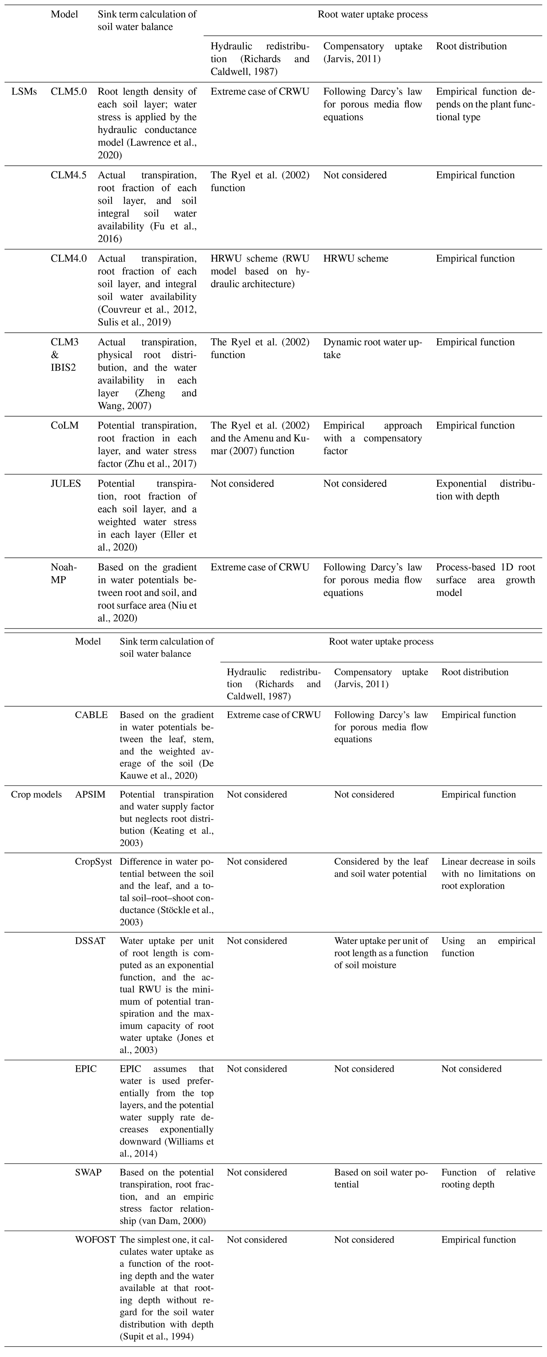
Because the spatial (i.e., 1D vertical) pattern of RWU is determined by the spatial distribution of the root system, knowledge of the latter is essential for predicting the spatial distribution of water contents and water fluxes in soils. The distribution of roots and their growth are, in turn, sensitive to various physical, chemical, and biological factors, as well as to soil hydraulic properties that influence the availability of water for plants (Beaudoin et al., 2009). Many attempts have been made in the past to develop root growth models that account for the influence of various environmental factors such as temperature, aeration, soil water availability, and soil compaction. Existing root growth models range from complex, 3D root architecture models (Bingham and Wu, 2011; Leitner et al., 2010; Wu et al., 2005) to much simpler root growth models that are implemented within more complex models such as EPIC (Williams et al., 1989) and DSSAT (Robertson et al., 1993). Most of these models reproduce the measured rooting depth very well, but the distribution of new growth root is based on empirical functions rather than biophysical processes (Camargo and Kemanian, 2016; Table 1).

Table 1 Comparison of land surface models (LSMs) and crop models in terms of sink term calculation of soil water balance. CRWU stands for compensatory root water uptake.

Modeling RWU requires the representation of above- and belowground processes, which can be realized considering the flow of water from soil through the plant to the atmosphere (i.e., the soil–plant–atmosphere continuum, SPAC model; Guo, 1992). The SPAC model represents a good compromise between simplicity (i.e., a small number of tuning parameters) and the ability to capture non-linear responses of RWU (and subsequently the ecosystem functioning) to drought events. Specifically, the SPAC model calculates the CRWU term using the gradient between the leaf water potential and the soil water potential of each soil layer. The most important parameters in the SPAC model include the leaf water potential, stomatal resistance, and the root resistance. Different from other macroscopic models using the root distribution function, the SPAC model explicitly needs the root length density at each soil layer to calculate the root resistance for each soil layer (Deng et al., 2017). The most practical method for obtaining the root length density is using a root growth model.

On other hand, remote sensing of solar-induced chlorophyll fluorescence (SIF) has been deployed to understand and monitor the ecosystem functioning under drought stress using models for vegetation photosynthesis and fluorescence (Zhang et al., 2018, 2020; Mohammed et al., 2019; Shan et al., 2019). SCOPE (Soil Canopy Observation, Photochemistry, and Energy Fluxes) is one such model and simulates canopy reflectance and fluorescence spectra in the observation directions as well as photosynthesis and evapotranspiration as functions of leaf optical properties, canopy structure, and weather variables (Van der Tol et al., 2009). The SCOPE model provides a valuable means to study the link between remote sensing signals and ecosystem functioning; however, it does not consider the water budget in soil and vegetation. As such, there is no explicit parametrization of the effects of soil moisture variations on the photosynthetic or stomatal parameters. Consequently, soil moisture effects are only “visible” in SCOPE if the lack of soil moisture affects the optical or thermal remote sensing signals (i.e., during water stress periods). The lack of such a link between soil moisture availability and remote sensing signals compromises the capacity of SCOPE to simulate and predict drought events on vegetation functioning.

The change in vegetation optical appearance as a result of soil moisture variations can only partially explain the soil moisture effect on ecosystem functioning (Bayat et al., 2018), which leads to considerably biased estimations of the gross primary productivity (GPP) and evapotranspiration (ET) under water-limited conditions. This presents a challenge with respect to using SCOPE for ecosystems in arid and semiarid areas, where water availability is the primary limiting factor for vegetation functioning. This challenge becomes even more relevant considering that soil moisture deficit or “ecological drought” is expected to increase in both frequency and severity in nearly all ecosystems around the world (Zhou et al., 2013). Bayat et al. (2019) incorporated the SPAC model into SCOPE to address water-stressed conditions at a grassland site, but the coupled model neglected the dynamic root distribution in different soil layers, and soil moisture only serves as a model input when it comes from measurements.

In this study, the modeling of aboveground photosynthesis, fluorescence emission, and energy fluxes in the vegetation layer by SCOPE will be fully coupled with a two-phase mass and heat transfer model – the STEMMUS model (Simultaneous Transfer of Energy, Mass and Momentum in Unsaturated Soil; a more detailed description of STEMMUS can be found in Sect. 2), by considering RWU based on a root growth model. The root growth model and the corresponding resistance scheme (from soil, through roots and leaves, to atmosphere) will be integrated for the dynamic modeling of water stress and the root system, enabling the seamless modeling of soil–water–plant energy, water, and carbon exchanges as well as SIF, thereby directly linking the vegetation dynamics (and its optical and thermal appearance) at the process level to soil moisture variability.

The rest of this article is structured as follows: Sect. 2 describes the coupling scheme between SCOPE and STEMMUS and the data that were used to validate the coupled model; Sect. 3 verifies the coupled STEMMUS–SCOPE model using a maize agroecosystem and a grassland ecosystem located in semiarid regions and explores the dynamic responses of the leaf water potential and root length density to water stress; and the summary of this study and the further challenges are addressed in Sect. 4.

2 Methodology and data

2.1 SCOPE and SCOPE_SM models

SCOPE is a radiative transfer and energy balance model (Van der Tol et al., 2009). It simulates the transfer of optical, thermal, and fluorescent radiation in the vegetation canopy and computes ET using an energy balance routine. SCOPE includes a radiative transfer module for incident solar and sky radiation to calculate the top-of-canopy outgoing radiation spectrum, net radiation, and absorbed photosynthetically active radiation (aPAR); a radiative transfer module for thermal radiation emitted by soil and vegetation to calculate the top-of-canopy outgoing thermal radiation and net radiation; an energy balance module for latent heat, sensible heat, and soil heat flux; and a radiative module for chlorophyll fluorescence to calculate the top-of-canopy SIF (the observation zenith angle was set as 0^∘ in this study).

Compared with other radiative transfer models that simplify the radiative transfer processes based on Beer's law, SCOPE has well-developed radiative transfer modules that consider the various leaf orientation and multiple scattering. SCOPE can provide detailed information about the net radiation of every leaf within the canopy. Furthermore, SCOPE incorporates an energy balance model that predicts not only the temperature of leaf but also the soil surface temperature (i.e., a vital boundary condition needed by STEMMUS). In the original SCOPE model, soil is treated in a very simple way with several empirical functions describing the ground heat storage. Later, Bayat et al. (2019) extended the SCOPE model by including the moisture effects on the vegetation canopy, which resulted in the SCOPE_SM model. This model takes soil moisture as input and predicts the effects on several processes of the vegetation canopy using the SPAC concept. Appendix A1 lists the main equations for calculating the water stress factor within SCOPE (Bayat et al., 2019), and the reader is referred to Van der Tol et al. (2009) for a detailed formulation of SCOPE.

SCOPE_SM provides the basic framework to couple SCOPE with a soil process model. However, both SCOPE and SCOPE_SM ignored the soil heat and mass transfer processes and the dynamics of root growth. This can be overcome by introducing the STEMMUS model.

2.2 STEMMUS model

The STEMMUS model is a two-phase mass and heat transfer model with explicit consideration of the coupled liquid, vapor, dry air, and heat transfer in unsaturated soil (Zeng et al., 2011a, b; Zeng and Su, 2013; Yu et al., 2016, 2018). STEMMUS provides a comprehensive description of water and heat transfer in the unsaturated soil, which can compensate for what is currently neglected in SCOPE. In STEMMUS, the soil layers can be set in a flexible manner, which is an improvement on the previous SPAC model that only considered the whole root zone soil water content as fixed layers (Williams et al., 1996). The water and heat transfer processes are vital for vegetation phenology development as well as freeze–thaw processes. The boundary condition needed by STEMMUS includes surface soil temperature, which is the output of SCOPE. In addition, STEMMUS already contains an empirical equation to calculate root water uptake and a simplified root growth module to calculate root fraction profile. As such, STEMMUS has an ideal model structure to be coupled with SCOPE. The main governing equations of STEMMUS are listed in Appendix A2.

2.3 Dynamic root growth and root water uptake

To obtain the root resistance of each soil layer, we incorporated a root growth module to simulate the root length density profile (see Appendix A3). The simulation of root growth refers to the root growth module in the INRA STICS crop growth model (Beaudoin et al., 2009), which includes the calculations of root front growth and root length growth. The root front growth is a function of temperature, with the depth of the root front beginning at the sowing depth for sown crops and at an initial value for transplanted crops or perennial crops (Beaudoin et al., 2009). The root length growth is calculated in each soil layer, considering the net assimilation rate and the allocation fraction of net assimilation to root, which is, in turn, a function of leaf area index (LAI) and root zone water content (Krinner et al., 2005). The root length density profile is then used to calculate the root resistance to water flow radially across the roots, soil hydraulic resistance, and plant axial resistance to flow from the soil to the leaves (see Appendix A4).

2.4 STEMMUS–SCOPE v1.0.0 coupling

The coupling starts with an initial soil moisture (SM) profile simulated by STEMMUS, which enables the calculation of the water stress factor as a reduction factor of the maximum carboxylation rate (V_cmax). SCOPE v1.73 is then used to calculate net photosynthesis (A_n) or gross primary productivity (GPP), soil respiration (R_s), energy fluxes (net radiation, R_n; latent heat, LE; sensible heat, H; and soil heat flux, G), transpiration (T), and SIF, which is passed to STEMMUS as the root water uptake (RWU). Then, the gross primary production (GPP) can be calculated based on A_n. Surface soil moisture is also used in calculating soil surface resistance and then calculating soil evaporation (E) . Furthermore, SCOPE can calculate soil surface temperature (T_s0) based on energy balance, which is subsequently used as the top boundary condition of STEMMUS, and leaf water potential (LWP), which is a parameter to reflect plant water status, can be calculated through iteration. Based on RWU, STEMMUS calculates the soil moisture in each layer at the end of the time step, and the new soil moisture profile will be the soil moisture at the beginning of next time step, which is repeated as such until the end of simulation period. The time step of STEMMUS–SCOPE is flexible, and the time step used in this study was 30 min. Figure 1 shows the coupling scheme of STEMMUS and SCOPE, and Table B1 in the Appendix shows all of the parameter values used in this study.

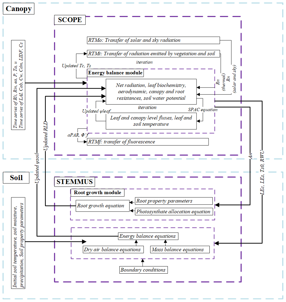
Figure 1 The coupling scheme of STEMMUS–SCOPE. Explanations for the symbols are given in Table B1 in the Appendix.

2.5 Evapotranspiration partitioning

Most studies in partitioning evapotranspiration (ET) use sap flow and microlysimeter data from in situ measurements. In this study, we used a simple and practical method to separate evaporation (E) and transpiration (T) proposed by Zhou et al. (2016). Although the behavior of plant stomata is influenced by environmental factors, the potential water use efficiency (uWUE_p, g C hPa^0.5 (kg H₂O)⁻¹) at the stomatal scale in the ecosystem with a homogeneous underlying surface is assumed to be nearly constant, and variations in actual uWUE (g C hPa^0.5 (kg H₂O)⁻¹) can be attributed to the soil evaporation (Zhou et al., 2016). Thus, the method can be used to estimate T and E with the quantities of ET, uWUE, and uWUE_p. Another assumption of this method is that the ecosystem T is equal to ET at some growth stages, so uWUE_p can be estimated using the upper bound of the ratio of $\text{GPP}\sqrt{\text{VPD}}$ to ET (here VPD refers to the vapor pressure deficit; Zhou et al., 2014, 2016).

Zhou et al. (2016) used the 95th quantile regression between $\text{GPP}\sqrt{\text{VPD}}$ and ET to estimate uWUE_p, and they showed that the 95th quantile regression for uWUE_p at flux tower sites was consistent with the uWUE derived at the leaf scale for different ecosystems. In addition, the variability in seasonal and interannual uWUE_p was relatively small for a homogeneous canopy. Therefore, the calculations of uWUE_p, uWUE, and T at the ecosystem scale were as follows:

$$\begin{array}{}\text{(1)}& {\displaystyle }& {\displaystyle }{\text{uWUE}}_{\mathrm{p}}={\displaystyle \frac{\text{GPP}\sqrt{\text{VPD}}}{T}}\text{(2)}& {\displaystyle }& {\displaystyle }\text{uWUE}={\displaystyle \frac{\text{GPP}\sqrt{\text{VPD}}}{\text{ET}}}\text{(3)}& {\displaystyle }& {\displaystyle \frac{T}{\text{ET}}}={\displaystyle \frac{\text{uWUE}}{{\text{uWUE}}_{\mathrm{p}}}}.\end{array}$$

The calculation of the VPD was based on air temperature and relative humidity data, and the method of gap-filling was the marginal distribution sampling (MDS) method proposed by Reichstein et al. (2005). To calculate GPP, the complete series of net ecosystem exchange (NEE) was partitioned into gross primary production (GPP) and respiration (Re) using the method proposed by Reichstein et al. (2005). Finally, ET was calculated using the latent heat flux and air temperature. Based on GPP, ET, and VPD data, T can be calculated using the method proposed by Zhou et al. (2016).

2.6 Study site and data description

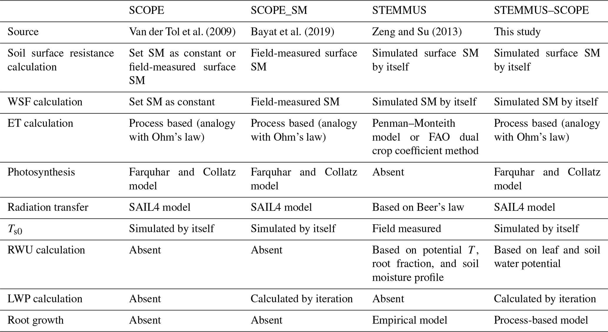
To evaluate the performance of STEMMUS–SCOPE in modeling ecohydrological processes, simulation was conducted to compare STEMMUS–SCOPE with SCOPE, SCOPE_SM, and STEMMUS using observations over a C₄ cropland (summer maize: from 11 June to 10 October 2017) at the Yangling station (34^∘17^′ N, 108^∘04^′ E; 521 m a.s.l.) and a C₃ grassland at the Vaira Ranch (US-Var) FLUXNET site (38^∘25^′ N, 120^∘57^′ W; 129 m a.s.l.; annual grasses: from 1 June to 8 August 2004). The seasonal variation in precipitation, irrigation, and SM for these two sites are presented in Fig. 2, and the differences in soil surface resistance, water stress factor (WSF), ET, photosynthesis, soil surface temperature (T_s0), root water uptake (RWU), and leaf water potential (LWP) between these four models are presented in Table 2. In this study, the LAI data of the Vaira Ranch (US-Var) FLUXNET site were from the MODIS 8 d LAI product instead of the field-measured LAI used by Bayat et al. (2019). For the soil water content employed by SCOPE_SM, the averaged root zone soil moisture was used for Yangling station, and the soil moisture at 10 cm depth was used for the Vaira Ranch site. For more detailed descriptions of these sites and data, the reader is referred to Wang et al. (2019, 2020a) and Bayat et al. (2018, 2019).

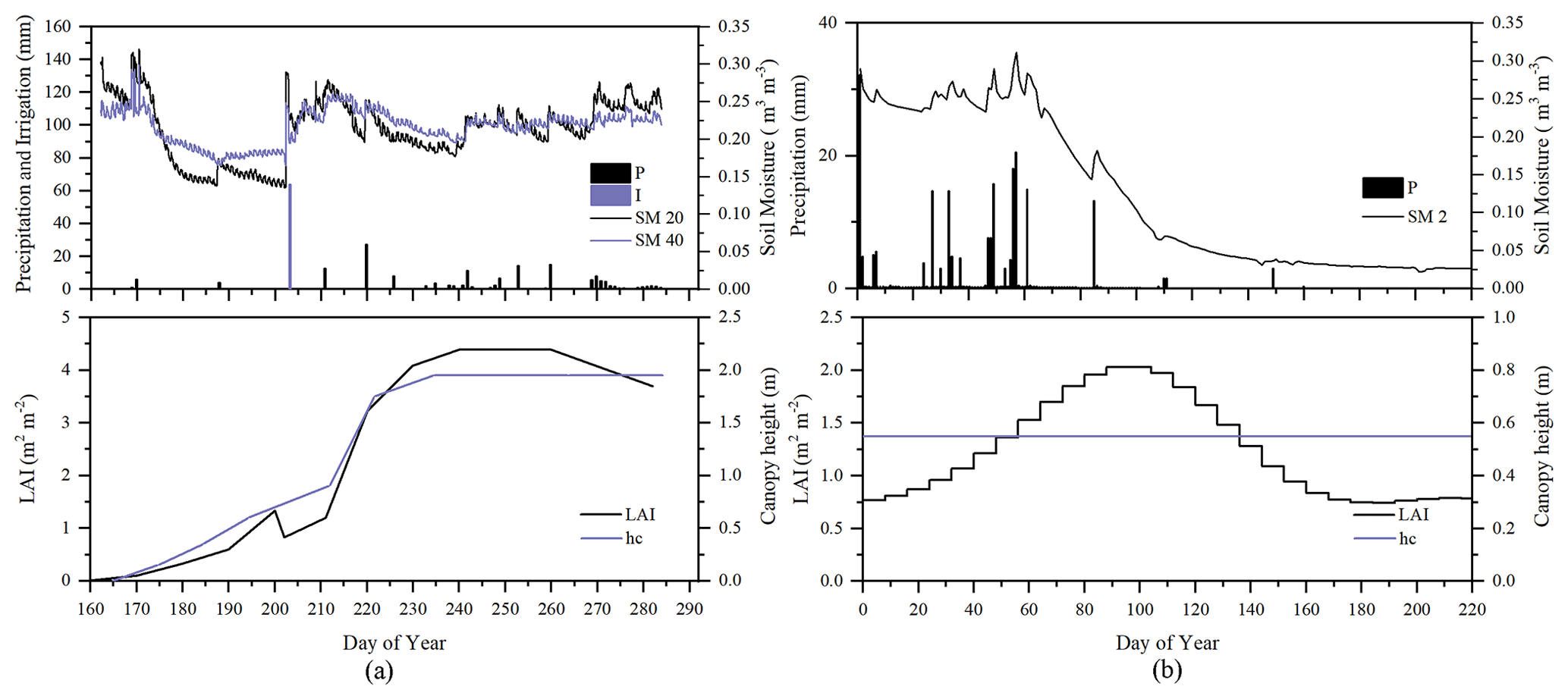
Figure 2 Seasonal variation in precipitation (P); irrigation (I); soil moisture at 2 (SM 2), 20 (SM 20), and 40 cm depth (SM 40); leaf area index (LAI); and canopy height (h_c) for (a) maize cropland at Yangling station and (b) grassland at the Vaira Ranch (US-Var) FLUXNET site.

Table 2 Main differences among SCOPE, SCOPE_SM, STEMMUS, and STEMMUS–SCOPE. The reader is referred to Table B1 in the Appendix for a description of the abbreviations used in this table.

2.7 Performance metrics

The metrics used to evaluate the performance of the coupled STEMMUS–SCOPE model include the (1) root-mean-square error (RMSE), (2) coefficient of determination (R²), and (3) the index of agreement (d). They are calculated as follows:

$$\begin{array}{}\text{(4)}& {\displaystyle }& {\displaystyle }\text{RMSE}=\sqrt{{\displaystyle \frac{\mathrm{1}}{n}}\sum _{i=\mathrm{1}}^n(P_i-O_i{)}^{\mathrm{2}}},\text{(5)}& {\displaystyle }& {\displaystyle }{R}^{\mathrm{2}}={\displaystyle \frac{{\left[\sum _{i=\mathrm{1}}^n(P_i-\overline{P})(O_i-\overline{O})\right]}^{\mathrm{2}}}{\sum _{i=\mathrm{1}}^n(P_i-\overline{P}{)}^{\mathrm{2}}{\sum }_{i=\mathrm{1}}^n(O_i-\overline{O}{)}^{\mathrm{2}}}},\text{(6)}& {\displaystyle }& {\displaystyle }d=\mathrm{1}-{\displaystyle \frac{\sum _{i=\mathrm{1}}^n(P_i-O_i{)}^{\mathrm{2}}}{\sum _{i=\mathrm{1}}^n(\left|P_i-\overline{O}\right|+\left|O_i-\overline{O}\right|{)}^{\mathrm{2}}}},\end{array}$$

where P_i is the ith predicted value, O_i is the ith observed value, $\overline{O}$ is the average of the observed values, and n is the number of samples.

3 Results and discussion

3.1 Soil moisture modeling

As the soil moisture profile was not available at the US-Var site, the comparisons of simulated soil moisture (SM) at Yangling station using STEMMUS and STEMMUS–SCOPE with observed values are presented in Fig. 3. For the simulation of soil moisture at 20 cm, the RMSE values were 0.023 and 0.021 and the d values were 0.90 and 0.91 for STEMMUS and STEMMUS–SCOPE, respectively. For the simulation of soil moisture at 40 cm, the RMSE values were 0.017 and 0.021 and the d values were 0.83 and 0.74, respectively. The simulated soil moisture at 20 cm depth agreed with the observed values in terms of the seasonal pattern. Although a slight overestimation occurred at initial and late stages, the dynamics in soil moisture resulting from precipitation or irrigation were well captured. Per the nature of the two models, the coupling of SCOPE with STEMMUS is not expected to improve the simulation of soil moisture. However, compared with SCOPE_SM, which used soil moisture measurements as inputs, the coupled STEMMUS–SCOPE model improves the simulation of soil moisture dynamics as measured. The deviation between the model simulations and the measurements can be attributed to the following two potential reasons. First, the field observations contain errors to a certain extent, and the soil moisture sensors may be not well calibrated. Second, in this simulation, we assumed that the soil texture was homogeneous in the vertical profile, whereas, in reality, the soil properties (e.g., soil bulk density and saturated hydraulic conductivity) may vary with depth and at different growth stages due to field management practices. For example, the soil bulk density at 40 cm was much higher than that at 20 cm due to the mechanical tillage, especially in the early stage.

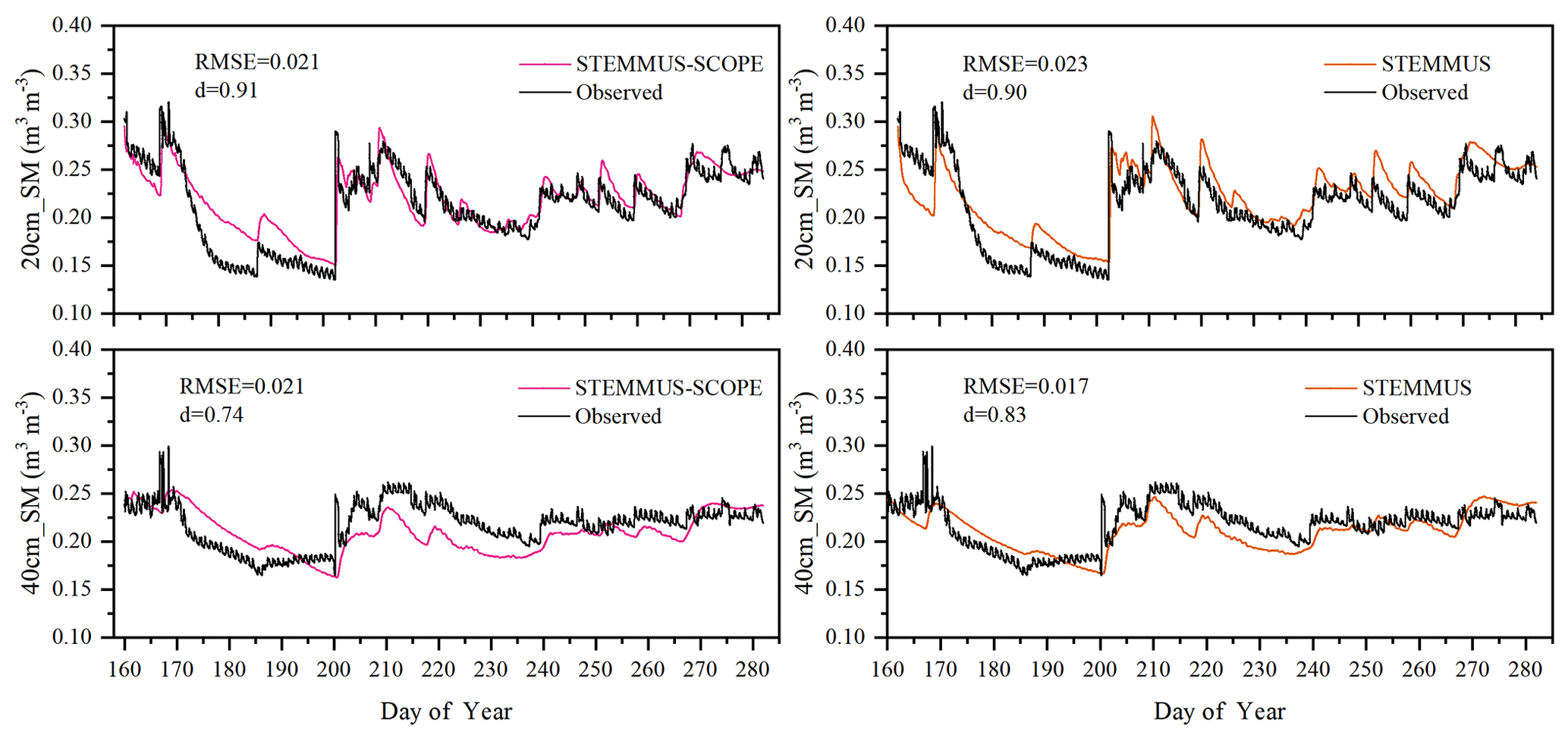
Figure 3 Comparison of modeled and observed soil moisture at 20 (20 cm_SM) and 40 cm (40 cm_SM) depth for the maize cropland at Yangling station.

3.2 Soil temperature modeling

Similar to soil moisture, only soil temperatures (T_s) simulated by STEMMUS and STEMMUS–SCOPE at 20 and 40 cm depth at the Yangling site are shown in Fig. 4. In general, both models can capture the dynamics of soil temperature well. For the simulation of temperature at 20 cm, the RMSE values were 2.56 and 2.58 ^∘C and the d values were 0.92 and 0.92 for STEMMUS and STEMMUS–SCOPE, respectively. For the simulation of temperature at 40 cm, the RMSE values were 2.06 and 2.07 ^∘C and the d values were 0.93 and 0.93, respectively. These results indicate that both models can simulate soil temperature well. However, some differences also exist between the simulation and observations. The largest difference occurred on DOY (day of year) 202, when the field was irrigated using the flood irrigation method. This irrigation activity may lead to boundary condition errors (i.e., for soil surface temperature), which cannot be estimated well enough (e.g., there is no monitoring of water temperature from the irrigation). Meanwhile, the measurements may also have some errors during this period. The fact that the observed soil temperature at 20 and 40 cm decreased to almost the same level at the same time indicates a potential pathway for preferential flow in the field (see precipitation and irrigation on DOY 202 in Fig. 2), and the sensors captured this phenomenon. Nevertheless, the model captures the soil temperature dynamics.

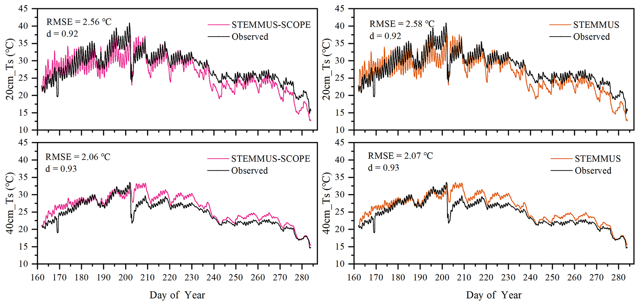
Figure 4 Comparison of observed and modeled soil temperature at 20 (20 cm_Ts) and 40 cm (40 cm_Ts) depth for the maize cropland at Yangling station.

3.3 Energy balance modeling

Comparisons of the modeled and observed 30 min net radiation (R_n), sensible heat flux (H), latent heat flux (LE), and soil heat flux (G) using SCOPE, SCOPE_SM, and STEMMUS–SCOPE are presented in Fig. 5 (STEMMUS uses R_n as driving data; therefore, it is not included in the comparison). For net radiation and soil heat flux, the simulations of all three models show good agreement with the observations, and the coefficients of determination (R²) for SCOPE, SCOPE_SM, and STEMMUS–SCOPE were 0.99, 1.00, and 0.99, respectively. For soil heat flux, the R² values for SCOPE, SCOPE_SM, and STEMMUS–SCOPE were 0.81, 0.79, and 0.80, respectively. For latent heat flux, STEMMUS–SCOPE shows better performance than SCOPE and SCOPE_SM, and the R² values for SCOPE, SCOPE_SM, and STEMMUS–SCOPE were 0.82, 0.84, and 0.85, respectively. Furthermore, STEMMUS–SCOPE and SCOPE_SM show similar performance in the simulation of sensible heat flux, both of which were better than the performance of SCOPE; the R² values for SCOPE, SCOPE_SM, and STEMMUS–SCOPE were 0.70, 0.75, and 0.74, respectively.

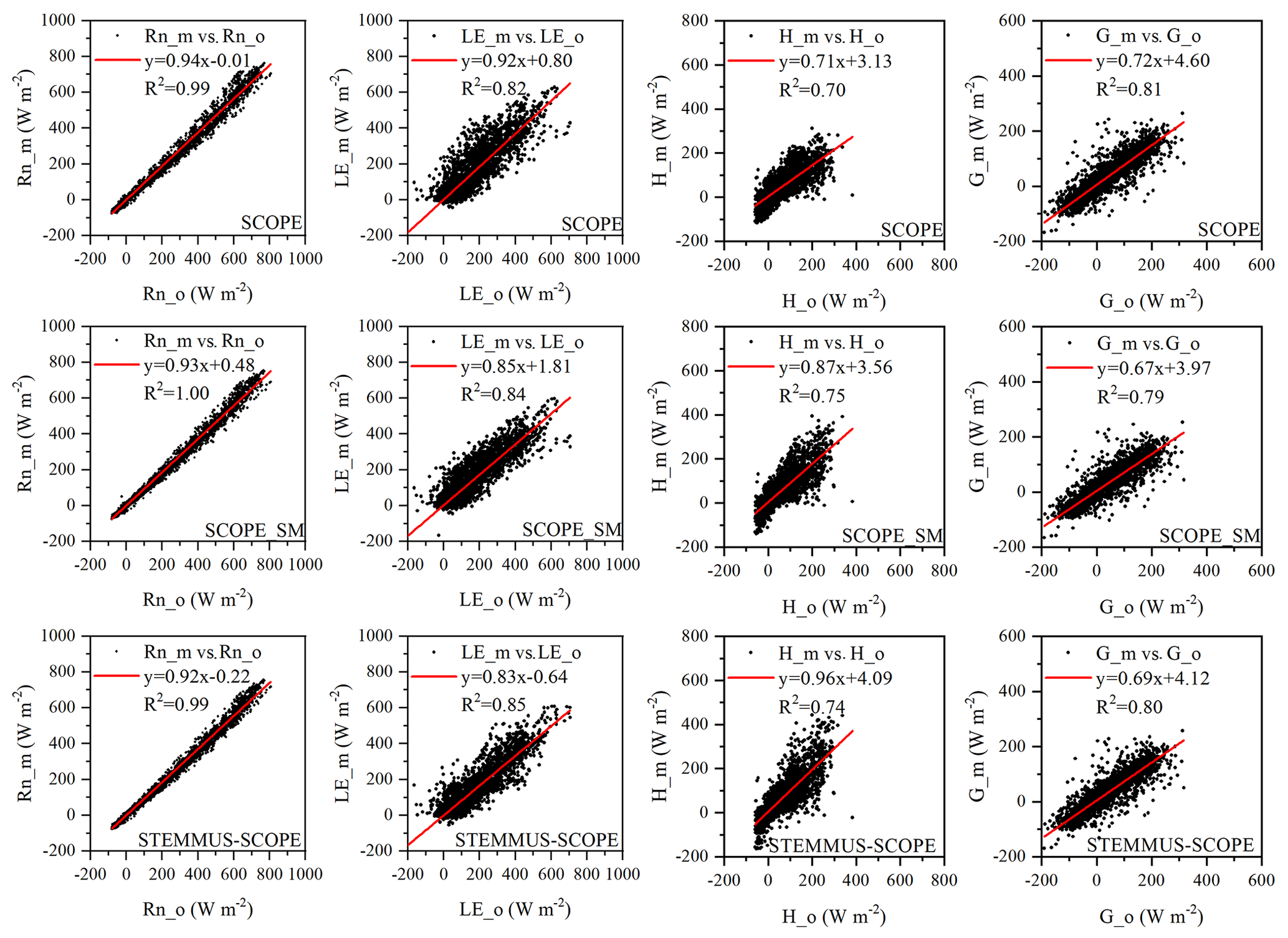
Figure 5 Comparison of modeled and observed 30 min net radiation (R_n), latent heat (LE), sensible heat (H), and soil heat flux (G) by SCOPE, SCOPE_SM, and STEMMUS–SCOPE at Yangling station. The subscripts “_m” and “_o” in each plot indicate modeled and observed quantities, respectively. The regression line is indicated in red, and the corresponding regression equation and R² value are given.

3.4 Daily ET, T, and E modeling

Simulated daily evapotranspiration (ET) results by SCOPE, SCOPE_SM, STEMMUS, and STEMMUS–SCOPE are presented in Fig. 6. For the Yangling station, the R² values for SCOPE, SCOPE_SM, STEMMUS, and STEMMUS–SCOPE were 0.76, 0.82, 0.80, and 0.81, and the RMSEs were 0.84, 0.69, 0.76, and 0.74 mm d⁻¹, respectively. For the US-Var station, the R² values for SCOPE, SCOPE_SM, STEMMUS, and STEMMUS–SCOPE were 0.10, 0.66, 0.84, and 0.89, and the RMSEs were 1.83, 0.63, 0.40, and 0.34 mm d⁻¹, respectively. For the ET simulation by SCOPE, there were large differences between simulations and observations when the vegetation suffered water stress. For SCOPE_SM, STEMMUS, and STEMMUS–SCOPE, the simulated ET values were closer to observations when the vegetation experienced water stress because the dynamics of soil moisture was included in the model. This indicates that STEMMUS–SCOPE, STEMMUS, and SCOPE_SM can predict ET with a relatively higher accuracy, especially when the maize was under water stress (DOY 183–202 at Yangling station and DOY 90–220 at the US-Var site), and STEMMUS–SCOPE and SCOPE_SM performed similarly well. It is noteworthy that although STEMMUS considered the effect of soil moisture on ET, the accuracy of STEMMUS was lower than that of the coupled model (see Fig. 6). The possible reason for this is the better representation of transpiration in the SCOPE model (see Fig. 7), which separates the canopy into 60 layers, whereas STEMMUS only treats the canopy as one layer. Moreover, the coupled model performed better for the grassland than for maize cropland. The reason for this is that the grassland simulation used the dynamic V_cmax data, whereas the maize simulation used a constant V_cmax data.

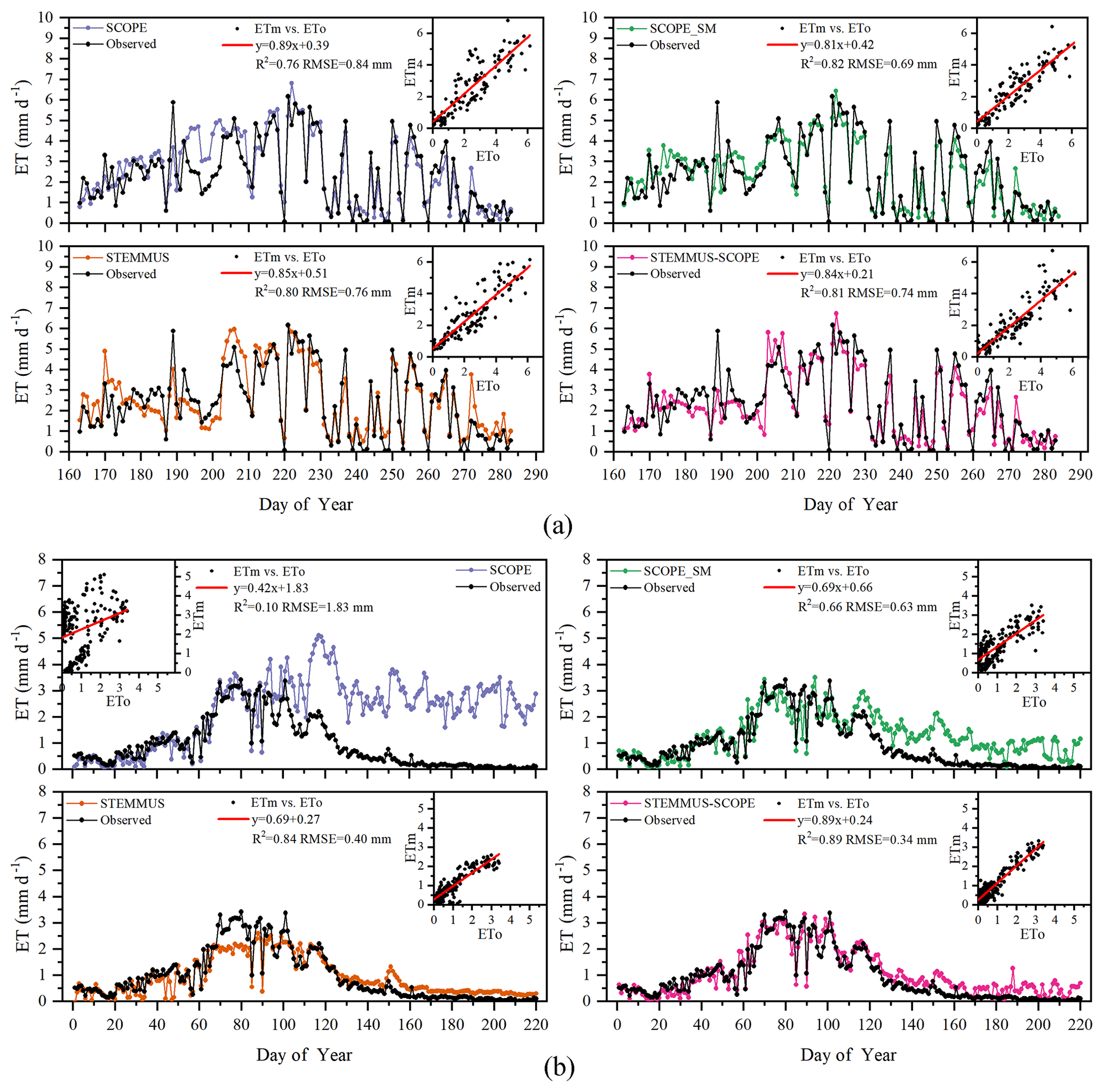
Figure 6 Comparison of modeled and observed daily evapotranspiration (ET) for (a) maize cropland at Yangling station and (b) grassland at the Vaira Ranch (US-Var) FLUXNET site (ETm denotes modeled ET, and ETo denotes observed ET).

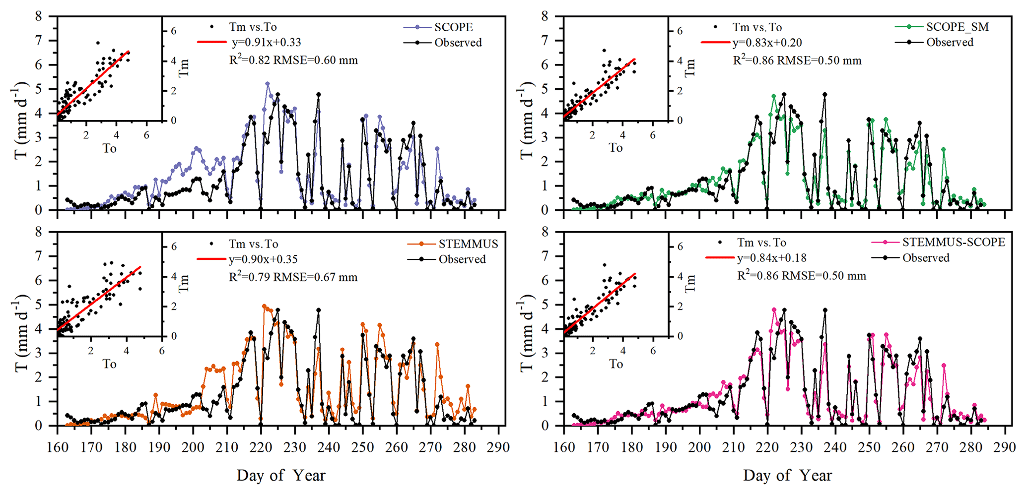
Figure 7 Comparison of modeled and observed daily plant transpiration (T) for the maize cropland at Yangling station (Tm denotes modeled T, and To denotes observed T).

The modeled and observed daily transpiration at the maize cropland are presented in Fig. 7, and the modeled transpiration at the grassland site is presented in Fig. 8. For Yangling station, the R² values between the simulated and observed transpiration were 0.82, 0.86, 0.79, and 0.86, and the RMSEs were 0.60, 0.50, 0.67, and 0.50 mm d⁻¹, for SCOPE, SCOPE_SM, STEMMUS, and STEMMUS–SCOPE, respectively. Because it ignored the effect of water stress on transpiration, SCOPE failed to simulate transpiration accurately when the vegetation experienced water stress. As shown in Fig. 6a, SCOPE overestimated transpiration for the maize cropland at Yangling station from DOY 183 to 202 during the water stress period. Compared with SCOPE, SCOPE_SM, STEMMUS, and STEMMUS–SCOPE can capture the reduction in transpiration during the dry period. The performance of STEMMUS–SCOPE and SCOPE_SM was also better than that of STEMMUS. The possible reason for this is the more processed-based consideration of the radiative transfer and energy balance at the leaf level in the coupled STEMMUS–SCOPE model (as in SCOPE_SM) and the more accurate root water uptake (compared with that in SCOPE_SM). Nevertheless, STEMMUS–SCOPE slightly underestimated transpiration when the plant was undergoing severe water stress and slightly overestimated it after the field was irrigated. This is mainly because the actual V_cmax was not only influenced by drought but was also related to the leaf nitrogen content (Xu and Baldocchi, 2003), which was not considered in the maize cropland simulation. Although measured T at the grassland was not available, we compared modeled T from the four models (Fig. 7). During the wet season (before DOY 85), the modeled T values from SCOPE, SCOPE_SM, and STEMMUS–SCOPE were similar and were higher than that from STEMMUS from DOY 64 to 82. During the dry season (after DOY 85), due to the simplified consideration of soil processes, the modeled T values from SCOPE and SCOPE_SM were both much higher than those from STEMMUS and STEMMUS–SCOPE. The reason for the better performance of the coupled model for the grassland (Fig. 6b) is that it also considers the effect of the leaf chlorophyll content (C_ab) on V_cmax, in addition to a more detailed consideration of water stress as discussed above for the maize cropland.

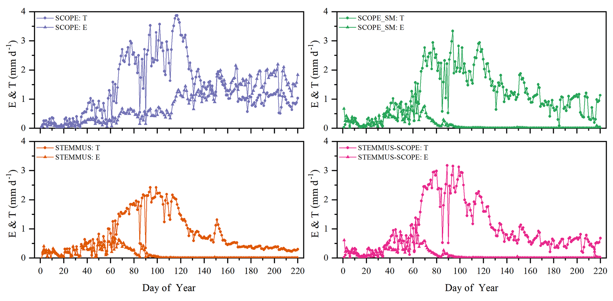
Figure 8 Comparison of modeled daily transpiration (T) and soil evaporation (E) for grassland at the Vaira Ranch (US-Var) FLUXNET site (T denotes transpiration, and E denotes soil evaporation).

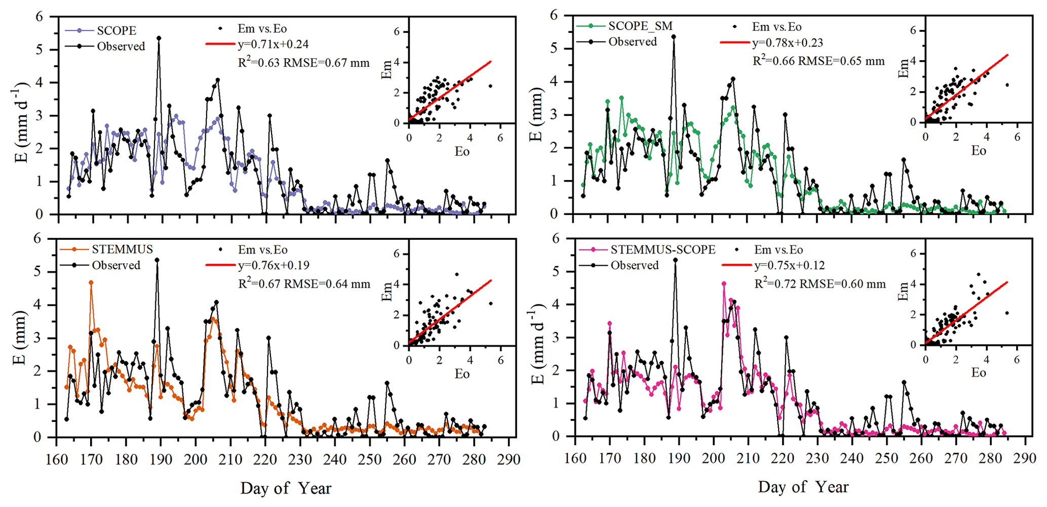
Figure 9 Comparison of modeled and observed daily soil evaporation (E) at Yangling station (Em denotes modeled E, and Eo denotes observed E).

As shown in Fig. 9 for soil evaporation at Yangling station, the simulated values from STEMMUS–SCOPE are closer to the observations than those from other models. When using SCOPE to simulate soil evaporation, the soil moisture is set as constant (i.e., 0.25 m³ m⁻³). Therefore, SCOPE generally underestimates soil evaporation when soil moisture is higher than 0.25 and overestimates it when it is lower than 0.25. Here, we use the average soil moisture at the root zone simulated by STEMMUS–SCOPE as the input data for SCOPE and SCOPE_SM in order to calculate soil surface resistance and soil evaporation. Although STEMMUS can capture variation in soil evaporation reasonably well, it has a higher RMSE than STEMMUS–SCOPE. This is probably attributed to the comprehensive consideration of radiation transfer in SCOPE, which is lacking in STEMMUS. Consequently, the simulation of soil net radiation by the coupled model was more accurate than that from STEMMUS alone. The RMSE value for STEMMUS–SCOPE was 0.60 mm d⁻¹, which was lower than those from the other three models (0.67, 0.65, and 0.64 mm d⁻¹, respectively). For STEMMUS–SCOPE, the major differences between simulations and observations occurred on rainy or irrigation days (see Fig. 2a), which may be caused by errors in the estimated soil surface resistance during these periods or the uncertainty of the ET partitioning method. The uncertainty of the ET partitioning method (Zhou et al., 2016) was mainly caused by (1) the uncertainty in the partitioning of GPP (less than 10 %) and Re based on NEE, which would result in some uncertainty in uWUE; (2) due to the seasonal variation in the atmospheric CO₂ concentration – the assumption of uWUE_p being constant would cause some uncertainty (less than 3 %); (3) the assumption of T being equal to ET sometimes during the growing season would cause some uncertainty when vegetation is sparse. Because the observed E at the US-Var site was not available, a comparison of only modeled E is shown in Fig. 8, in which SCOPE modeled unrealistic E during the dry season, whereas the modeled E values from SCOPE_SM, STEMMUS, and STEMMUS–SCOPE were consistent due to the use the simulated surface SM as the input for soil evaporation calculation.

3.5 Daily GPP modeling

Simulated GPP from SCOPE, SCOPE_SM, and STEMMUS–SCOPE and observed GPP are presented in Fig. 10. As shown, similar to the simulation of transpiration, SCOPE cannot respond to water stress when simulating GPP. After introducing a soil water stress factor in STEMMUS–SCOPE and SCOPE_SM, the simulation of GPP was improved in both models. For Yangling station, the consistency between simulated and observed GPP at mid and late stages was higher than that at early and rapid growth stages. The difference usually occurred when soil moisture increased. For the US-Var site, STEMMUS–SCOPE simulated GPP well during the whole period, whereas SCOPE_SM slightly underestimated GPP around DOY 80 when this site transits from the wet season to the dry season. This indicates that only using the surface SM cannot reflect the actual root zone SM when the vegetation is experiencing moderate water stress. Under such conditions, the hydraulic redistribution (HR) and compensatory root water uptake (CRWU) process enable the vegetation to utilize the water in the deep soil layer. Only using the surface soil water content to calculate RWU in SCOPE_SM ignored the effect of the HR and CRWU process, and the effect of water stress was overestimated. However, the surface soil moisture can reflect root zone soil moisture well when the vegetation is not under water stress or severe water stress. A similar underestimation of GPP was also found by Bayat et al. (2019).

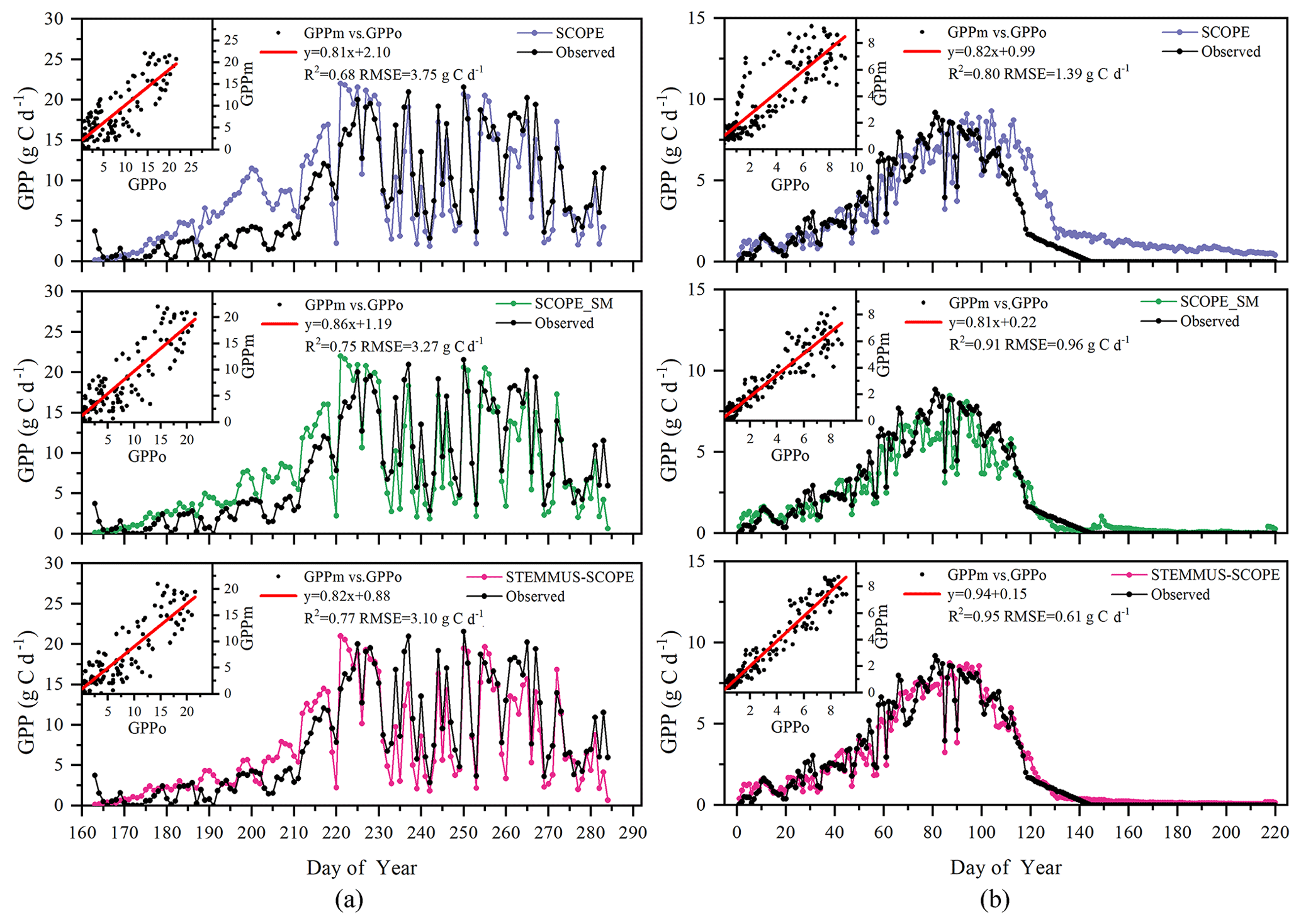
Figure 10 Comparison of modeled and observed daily gross primary production (GPP) for (a) maize cropland at Yangling station and (b) grassland at the Vaira Ranch (US-Var) FLUXNET site (GPPm denotes modeled GPP, and GPPo denotes observed GPP).

3.6 Simulation of leaf water potential (LWP), water stress factor (WSF), and root length density (RLD)

The simulated 30 min leaf water potential and water stress factor at Yangling station are presented in Fig. 11. The leaf water potential was lower when vegetation was suffering water stress compared with other periods. The reason for this is that soil water potential is low due to the low soil moisture, and plants need to maintain an even lower leaf water potential to suck water from the soil and transfer it to leaves. During mid and late stages, the leaf water potential was sensitive to transpiration demand due to the slowdown of root system growth. As continuous measurements of the leaf water potential are not available, we compared only the magnitude of simulated leaf water potential to measurements reported in the literature.

Figure 11 Simulation of ψ_leaf (leaf water potential, m) and the WSF (water stress factor) at Yangling station. (The dotted lines represent the range of midday leaf water potential reported at other sites.)

Many studies have measured midday leaf water potential or dawn leaf water potential. Fan et al. (2015) reported that the leaf water potential of well-watered maize remained high at between −73 and −88 m and that leaf water potential would decrease when the soil water content was lower than 80 % of field capacity. Martineau et al. (2017) reported that the midday leaf water potential of well-watered maize was around −0.82 MPa (about 84.8 m in water pressure head; note that 0.1 MPa is equal to 10.339 m water pressure head) and that the midday leaf water potential decreased to −1.3 MPa (about 134.4 m in water head) when the maize was suffering water stress. Moreover, O'Toole and Cruz (1980) studied the response of leaf water potential to water stress in rice and concluded that the leaf water potential of rice can be lower than −80 to −120 m when the vegetation was under water stress and the leaves started curling, which was similar to the simulated leaf water potential of maize in this study. Aston and Lawlor (1979) revealed the relationship between transpiration, root water uptake, and leaf water potential of maize. These field studies found that leaf water potential was often very low and reached trough values at midday. Elfving et al. (1972) developed a water flux model based on the SPAC system, evaluated it for orange trees, and reported about −120 m for the trough value of leaf water potential under non-limiting environmental conditions, which was slightly lower than the simulation in this study.

In this study, the calculation of the water stress factor considered the effect of soil moisture and root distribution. The severe water stress occurred from DOY 183 to 202, and the coupled model performed very well during this period. Due to feedback, water stress can also influence root water uptake and root growth and, consequently, influence soil moisture and root dynamics in next time step. This indicates that the water stress equation used in this study can characterize the reduction in V_cmax reasonably well.

Root length density is another vital parameter in calculating root water uptake. As shown in Table 3, the simulated peak root length density and maximum rooting depth of maize at Yangling station was comparable to the measured values from other sites. Many previous studies have revealed that root length density is influenced by soil moisture, bulk density, tillage, and soil mineral nitrogen (Amato and Ritchie, 2002; Chassot et al., 2001; Schroder et al., 1996). In this study, as we assumed that the soil was homogenous. STEMMUS–SCOPE considered the effect of soil moisture but neglected the effect of bulk density and soil mineral nitrogen. Amato and Ritchie (2002) also found a similar result to this study with respect to the root length density in a maize field. Peng et al. (2012) studied temporal and spatial dynamics in the root length density of field-grown maize and found that 80 % root length density was distributed at 0–30 cm depth with peak values from 0.86 to 1.00 cm cm⁻³. Ning et al. (2015) also reported a similar observation of root length density. Chassot et al. (2001) and Qin et al. (2006) reported that root length density can reach 1.59 cm cm⁻³ in the Swiss Midlands. In Stuttgart, Germany, Wiesler and Horst (1994) observed the root growth and nitrate utilization of maize under field conditions. The observed root length density was 2.45–2.80 cm cm⁻³ at 0–30 cm depth, which was much higher than in other studies, and decreased to 0.01 cm cm⁻³ at 120–150 cm depth, which was consistent with the observations of Oikeh et al. (1999) at Samaru, Nigeria. Zhuang et al. (2001b) proposed a scaling model to estimate the distribution of the root length density of field-grown maize. In their study, the measured root length density in Tokyo, Japan, decreased from 0.4 to 0.95 cm cm⁻³ in the top soil layer to about 0.1 cm cm⁻³ in the bottom layer. Zhuang et al. (2001a) observed that the root length density of maize was mainly distributed at 0–60 cm depth, and the maximum values were about 0.9 cm cm⁻³. These studies indicated that the root length density values were quite variable when this parameter was observed at different sites; nevertheless, the simulated root length density in our study was of an order of magnitude that was similar to the observations from previous studies (Table 3).

Table 3 Comparison of the peak root length density (RLD; cm cm⁻³) at Yangling station with that at other sites.

3.7 Diurnal variation in T, GPP, SIF, and LWP

Figure 12 shows the modeled and observed 30 min canopy transpiration (T), gross primary production (GPP), solar-induced fluorescence (SIF), and leaf water potential (LWP) from DOY 183 to 202 at Yangling station. The simulations by STEMMUS–SCOPE and SCOPE_SM were consistent with observations, whereas the simulated values from SCOPE were much higher than observations. The performance of STEMMUS–SCOPE and SCOPE_SM was consistent with that of SCOPE in the early morning and late afternoon, when photosynthesis was mainly limited by incident radiation rather than by water stress, intercellular CO₂ concentration, and V_cmax. At midday, with increasing incident radiation, photosynthesis was mainly limited by water stress and V_cmax, during which time the simulations by STEMMUS–SCOPE and SCOPE_SM were much better than that by SCOPE. The diurnal variation in the observed and modeled GPP was similar to that of T. Due to the lack of observed SIF, only the simulated SIF values were presented. As shown in Fig. 12, the SIF values simulated by STEMMUS- SCOPE and SCOPE_SM were reduced when the vegetation was experiencing water stress, which indicated that both the simulated SIF from STEMMUS–SCOPE and SCOPE_SM can respond to water stress. However, the accuracy of the simulated SIF requires further validation with field observations.

Figure 12 Comparison of modeled and observed 30 min transpiration (T), gross primary production (GPP), top-of-canopy solar-induced fluorescence (SIF), and leaf water potential (LWP) at Yangling station.

Figure 13 shows the relationship among 30 min GPP, SIF, and LWP on DOY 199 at Yangling station. There was a strong linear relationship between SIF and GPP when the maize was well-watered (Fig. 13a). However, SIF kept increasing, whereas GPP tended to saturate when the maize was suffering water stress. This result is consistent with the previous study conducted for cotton and tobacco leaves (Van der Tol et al., 2014). Because SCOPE_SM used the averaged root zone SM and ignored vertical root and soil water distribution, it overestimated GPP and SIF. When the maize was experiencing drought, the LWP was maintained at a low level. With GPP and T increasing, the plant decreased LWP in order to extract enough water from the root zone. The SPAC system enabled STEMMUS–SCOPE to simulate 30 min LWP. To better detect the response of simulated SIF to simulated LWP, we chose a cloudless day (DOY 199), and a liner relationship between the simulated SIF and LWP was obtained (Fig. 13b). Sun et al. (2016) reported that the SIF–soil moisture–drought relationship depended on variations in both absorbed PAR and fluorescence yield in response to water stress, whereas the LWP can reflect both the effect of absorbed PAR and the soil moisture status. The strong correlation between GPP, LWP, and SIF indicates the potential for using SIF as an effective signal for characterizing the response of photosynthesis to water stress. In the future, more studies should focus on the measurement of SIF, GPP, and LWP simultaneously for different vegetation types across different environmental conditions (radiation, soil moisture, and CO₂ concentration) to reveal how the water stress affects these relationships.

Figure 13 The relationship among gross primary production (GPP), top-of-canopy solar-induced fluorescence (SIF), and leaf water potential (LWP) on DOY 199: (a) GPP vs. SIF; (b) SIF vs. LWP.

3.8 Limitations that need to be overcome

The new coupled model notably improved simulations of carbon and water fluxes when vegetation was suffering water stress. However, this study mainly aimed to improve the response of SCOPE to drought by introducing the vertical soil water and root profile. Some critical processes were followed that existed in SCOPE_SM and STEMMUS. As with any model, some modules in STEMMUS–SCOPE, such as plant hydraulics and root growth, could be improved upon in future development.

First, to date many LSMs (e.g., CLM 5, Noah-MP, JULES, and CABLE) have incorporated a state-of-the-art plant hydraulics model to replace the conventional empirical plant hydraulic model which was only based on the distribution of SM and the fraction of roots (e.g., CLM 4.5 and CoLM; De Kauwe et al., 2015). Although STEMMUS–SCOPE integrated a 1D root growth model and a relatively novel RWU model, its hydraulics model followed that in SCOPE_SM and ignored the most exciting recent advances in our understanding of plant hydraulics: hydraulic failure due to the loss of hydraulic conductivity owing to embolism and refilling for recovery from xylem embolism (McDowell et al., 2019). Because STEMMUS–SCOPE performed well in maize cropland and grassland, the influence of embolism and refilling on water transfer from the soil through vegetation to the atmosphere cannot be fully detected. The value of using plant water potential instead of soil water potential to constrain model predictions has been demonstrated in many case studies (De Kauwe et al., 2020; Niu et al., 2020; Medlyn et al., 2016; Xu et al., 2016; Williams et al., 1996). Niu et al. (2020) followed the plant hydraulic model developed by Xu et al. (2016) and represented the plant stomatal water stress factor as a function of the plant water storage. CLM 5.0 also introduced a new formulation for WSF, which is based on leaf water potential (ψ_leaf) instead of soil water potential (ψ_soil; Kennedy et al., 2019). These new formulations based on plant water potential could offer significant improvements for plant drought responses. Furthermore, STEMMUS–SCOPE presently does not account for plant water storage; this may result in underestimating morning LE and overestimating afternoon LE. Some field observations have shown that the plant do not immediately respond when soil moisture is enhanced (Mackay et al., 2019), instead there are long lags, which were ignored in this study, between soil water recovery from drought and plant responses to the recovery. The WSF in STEMMUS–SCOPE directly comes from soil moisture and cannot reflect true stomatal response when vegetation is experiencing drought. For example, in early morning, the low stomatal aperture was induced by low PAR rather than by SM. Consequently, STEMMUS–SCOPE needs to introduce advanced hydraulics after the model has been tested in a wide range of ecosystems, particularly for vegetation exposed to frequent drought cycles or prolonged periods of severe drought events. It is important, however, to note that explicit representations of plant hydraulics require additional model parameters and increase the parameterization burden. This is the most challenging limitation to STEMMUS–SCOPE with respect to incorporating these hydraulics models, and we have chosen a trade-off between mechanism and practicality.

Second, as mentioned above, STEMMUS–SCOPE adapted the macroscopic RWU model and a simplified 1D root growth model in order to save on computational costs, although it predicted maximum root depth well, which is the most critical factor when calculating WSF and RWU. Such a simplification would likely ease the migration of our model into larger-scale models, such as Earth system models. However, STEMMUS–SCOPE oversimplified metabolic processes of the roots, including root exudates, root maintenance respiration, root growth respiration, and root turnover, which are also critical and have been incorporated in Noah-MP (Niu et al., 2020). This simplification could result in uncertainties in modeling the root growth and root water uptake. Meanwhile, there was no validation of the seasonal vertical root length distribution based on in situ observations, which need to be validated in the next step. Furthermore, the model presently does not account for the feedback between hydraulic controls over carbon allocation and the role of root growth on soil–plant hydraulics, which could also be considered in future model development.

4 Conclusions

A fundamental understanding of coupled energy, water, and carbon flux is vital for obtaining information on ecohydrological processes and functioning under climate change. The coupled model, STEMMUS–SCOPE, integrating radiative transfer, photochemistry, energy balance, root system dynamics, and soil moisture and soil temperature dynamics, has been proven to be a practical model to simulate detailed land surface processes such as evapotranspiration and GPP. In the coupled model, STEMMUS could provide the root zone moisture profile to SCOPE, which was used to calculate the water stress factor. On the other hand, SCOPE could provide the net carbon assimilation and soil surface temperature to STEMMUS, which was subsequently used as the top boundary condition and as the input for root growth model. This study explores the role of dynamic root growth in affecting canopy photosynthesis activities, fluorescence emissions, and evapotranspiration, which has not been reported before. The coupled model has been successfully applied in a maize field and a grassland and can be used to describe ET partitioning, canopy photosynthesis, reflectance, and fluorescence emissions. The results show that by considering dynamic root growth and the associated root water uptake, the simulated SIF of the coupled STEMMUS–SCOPE model can respond to water stress, whereas this is not the case for SCOPE_SM. Through the intercomparison of SCOPE, SCOPE_SM, STEMMUS, and STEMMUS–SCOPE, we concluded that the coupled STEMMUS–SCOPE model can be used to investigate vegetation states under water-stressed conditions and to simultaneously understand the dynamics of soil heat and mass transfer, as well as the root growth. By considering the vertical distribution of soil moisture and the root system, the simulation of water and carbon fluxes, especially when vegetation was suffering moderate water stress, was significantly improved. However, the need remains for further studies to enhance the capacity of STEMMUS–SCOPE with respect to understanding ecosystem functioning. First of all, the estimation of the soil boundary condition, especially during the irrigation period, which has a significant influence on the simulation of soil temperature, requires further consideration. Second, the realism of the present model in modeling the water-stressed SIF will be subject to further studies. Nevertheless, STEMMUS–SCOPE may be used as an effective forward simulator to simulate remote sensing signals and to assimilate remote sensing data, such as solar-induced chlorophyll fluorescence, in order to improve the estimation of water and carbon fluxes. STEMMUS–SCOPE could also be used to investigate regional or global land surface processes, especially in arid and semiarid regions, due to its sensitivity to water-stressed conditions.

Appendix A

A1 Photosynthesis and evapotranspiration under water stress in SCOPE

The C₄ photosynthesis is calculated in the SCOPE model as the minimum of three processes (Collatz et al., 1991, 1992): (1) the carboxylation rate limited by ribulose bisphosphate–carboxylase–oxygenase activity (known as rubisco (enzyme) limited), V_c, described in Eq. (A1); (2) the carboxylation rate limited by ribulose 1–5 bisphosphate regeneration rate (known as RuBP (electron transport/light) limited), V_e, described in Eq. (A2); and (3) at low CO₂ concentrations, the carboxylation rate limited by intercellular CO₂ partial pressure (p_i), V_s, described in Eq. (A3).

$$\begin{array}{}\text{(A1)}& {\displaystyle }& {\displaystyle }{V}_{\mathrm{c}}=V_{\text{cmax}}\cdot \text{WSF}\text{(A2)}& {\displaystyle }& {\displaystyle }{V}_{\mathrm{e}}={\displaystyle \frac{J}{\mathrm{6}}}{\displaystyle \frac{-b\pm \sqrt{b^{\mathrm{2}}-\mathrm{4}ac}}{\mathrm{2}a}}\text{(A3)}& {\displaystyle }& {\displaystyle }{V}_{\mathrm{s}}=p_i\left(k_{\mathrm{p}}-{\displaystyle \frac{L}{p_i}}\right)/P\text{(A4)}& {\displaystyle }& {\displaystyle }{A}_{\mathrm{n}}=min\left(V_{\mathrm{c}},V_{\mathrm{e}},V_{\mathrm{s}}\right)\end{array}$$

The C₃ photosynthesis is calculated in the SCOPE model as the minimum of two processes (Farquhar et al., 1980): (1) the carboxylation rate limited by ribulose bisphosphate–carboxylase–oxygenase activity (known as rubisco (enzyme) limited), V_c, described in Eq. (A5); and (2) the carboxylation rate limited by ribulose 1–5 bisphosphate regeneration rate (known as RuBP (electron transport/light) limited), V_e, described in Eq. (A6).

$$\begin{array}{}\text{(A5)}& {\displaystyle }& {\displaystyle }{V}_{\mathrm{c}}=V_{\text{cmax}}\cdot \text{WSF}\cdot {\displaystyle \frac{C_i-{\mathrm{\Gamma }}^{\ast }}{C_i+K_{\mathrm{c}}(\mathrm{1}+\frac{O_i}{K_{\mathrm{o}}})}}\text{(A6)}& {\displaystyle }& {\displaystyle }{V}_{\mathrm{e}}={\displaystyle \frac{J(C_i-{\mathrm{\Gamma }}^{\ast })}{\mathrm{4}(C_i+\mathrm{2}{\mathrm{\Gamma }}^{\ast })}}{\displaystyle \frac{-b\pm \sqrt{b^{\mathrm{2}}-\mathrm{4}ac}}{\mathrm{2}a}}\text{(A7)}& {\displaystyle }& {\displaystyle }{A}_{\mathrm{n}}=min\left(V_{\mathrm{c}},V_{\mathrm{e}}\right)\text{(A8)}& {\displaystyle }& {\displaystyle }{C}_i=C_{\mathrm{a}}\left(\mathrm{1}-{\displaystyle \frac{\mathrm{1}}{m\text{RH}}}\right)\end{array}$$

Here, V_cmax is the maximum carboxylation rate ($\mathrm{\mu }\mathrm{mol}{\mathrm{m}}^{-\mathrm{2}}{\mathrm{s}}^{-\mathrm{1}}$), p_i is the intercellular CO₂ partial pressure (Pa), k_p is a pseudo-first-order rate constant for PEP carboxylase with respect to C_i, P is the atmospheric pressure, A_n is the net photosynthesis ($\mathrm{\mu }\mathrm{mol}{\mathrm{m}}^{-\mathrm{2}}{\mathrm{s}}^{-\mathrm{1}}$), WSF is the total water stress factor, J is the electron transport rate ($\mathrm{\mu }\mathrm{mol}{\mathrm{m}}^{-\mathrm{2}}{\mathrm{s}}^{-\mathrm{1}}$), C_i is the intercellular CO₂ concentration (µmol m⁻³), C_a is CO₂ concentration in the boundary layer (µmol m⁻³), m is Ball–Berry parameter, and RH is relative humidity at the leaf surface (%).

In addition, leaf stomatal resistance r_c (s m⁻¹) is calculated as

$$\begin{array}{}\text{(A9)}& r_{\mathrm{c}}={\displaystyle \frac{\mathrm{0.625}(C_{\mathrm{s}}-C_i)}{A_{\mathrm{n}}}}{\displaystyle \frac{{\mathit{\rho }}_{\mathrm{a}}}{M_{\mathrm{a}}}}{\displaystyle \frac{{\mathrm{10}}^{\mathrm{12}}}{p}},\end{array}$$

where ρ_a is specific mass of air (kg m⁻³), M_a is molecular mass of dry air (g mol⁻¹), and p is atmosphere pressure (hPa).

The calculation of latent heat flux (LE) is as follows:

$$\begin{array}{}\text{(A10)}& LE=\mathit{\lambda }{\displaystyle \frac{(q_i-q_{\mathrm{a}})}{r_{\mathrm{a}}+r_{\mathrm{c}}}},\end{array}$$

where λ is vaporization heat of water (J kg⁻¹), q_i is the humidity in stomata or soil pores (kg m⁻³), q_a is the humidity above the canopy (kg m⁻³), r_c is stomatal or soil surface resistance (s m⁻¹), and r_a is aerodynamic resistance (s m⁻¹).

In the study of Bayat et al. (2019), the water stress factor was calculated based on the root zone soil moisture content neglecting the distribution of root length. In this study, the water stress factor considered both root length distribution and water content in root zone. We use a sigmoid formulation rather than the piecewise function by Bayat et al. (2019). The calculations are as follows:

$$\begin{array}{}\text{(A11)}& {\displaystyle }& {\displaystyle }\text{WSF}={\sum }_{i=\mathrm{1}}^n\text{RF}\left(i\right)\cdot \text{WSF}\left(i\right)\text{(A12)}& {\displaystyle }& {\displaystyle }\text{WSF}\left(i\right)={\displaystyle \frac{\mathrm{1}}{\mathrm{1}+e^{-\mathrm{100}\cdot {\mathit{\theta }}_{\text{sat}}\left(\text{SM}\left(i\right)-\frac{{\mathit{\theta }}_{\mathrm{f}}+{\mathit{\theta }}_{\mathrm{w}}}{\mathrm{2}}\right)}}}\end{array}$$

where θ_w is the soil water content at wilting point, θ_f is the soil water content at field capacity, θ_sat is the saturated soil water content, WSF(i) is the water stress factor at each soil layer, RF(i) is the ratio of root length in soil layer i (its calculation can be found in the Appendix A4), and SM(i) is the soil moisture at each soil layer.

A2 Governing equations in STEMMUS

A2.1 Soil water conservation equation

The soil water conservation equation is as follows:

$$\begin{array}{ll}\text{(A13)}& {\displaystyle }& {\displaystyle \frac{\partial }{\partial t}}\left({\mathit{\rho }}_{\mathrm{L}}{\mathit{\theta }}_{\mathrm{L}}+{\mathit{\rho }}_{\mathrm{V}}{\mathit{\theta }}_{\mathrm{V}}\right){\displaystyle }& {\displaystyle }=-{\displaystyle \frac{\partial }{\partial z}}\left(q_{\text{Lh}}+q_{\text{LT}}+q_{\text{La}}+q_{\text{Vh}}+q_{\text{VT}}+q_{\text{Va}}\right)-S\\ {\displaystyle }& {\displaystyle }={\mathit{\rho }}_{\mathrm{L}}{\displaystyle \frac{\partial }{\partial z}}[K\left({\displaystyle \frac{\partial h}{\partial z}}+\mathrm{1}\right)\\ {\displaystyle }& {\displaystyle }+D_{\text{TD}}{\displaystyle \frac{\partial T_{\mathrm{s}}}{\partial z}}+{\displaystyle \frac{K}{{\mathit{\gamma }}_{\mathrm{w}}}}{\displaystyle \frac{\partial P_{\mathrm{g}}}{\partial z}}]\\ {\displaystyle }& {\displaystyle }+{\displaystyle \frac{\partial }{\partial z}}\left[D_{\text{Vh}}{\displaystyle \frac{\partial h}{\partial z}}+D_{\text{VT}}{\displaystyle \frac{\partial T_{\mathrm{s}}}{\partial z}}+D_{\text{Va}}{\displaystyle \frac{\partial P_{\mathrm{g}}}{\partial z}}\right]-S,\end{array}$$

where ρ_L and ρ_V (kg m⁻³) are the density of liquid water and water vapor, respectively; q_L and q_V (m³ m⁻³) are the volumetric water content for liquid and water vapor, respectively; z(m) is the vertical space coordinate (positive upwards); S (cm s⁻¹) is the sink term for the root water extraction; K (m s⁻¹) is hydraulic conductivity; h (cm) is the pressure head; T_s (^∘C) is the soil temperature; P_g (Pa) is the mixed pore-air pressure; γ_w ($\mathrm{kg}{\mathrm{m}}^{-\mathrm{2}}{\mathrm{s}}^{-\mathrm{2}}$) is the specific weight of water; D_TD ($\mathrm{kg}{\mathrm{m}}^{-\mathrm{1}}{\mathrm{s}}^{-\mathrm{1}}({}^{\circ }\mathrm{C}{)}^{-\mathrm{1}}$) is the transport coefficient for adsorbed liquid flow due to the temperature gradient; D_Vh ($\mathrm{kg}{\mathrm{m}}^{-\mathrm{2}}{\mathrm{s}}^{-\mathrm{1}}$) is the isothermal vapor conductivity; D_VT ($\mathrm{kg}{\mathrm{m}}^{-\mathrm{1}}{\mathrm{s}}^{-\mathrm{1}}({}^{\circ }\mathrm{C}{)}^{-\mathrm{1}}$) is the thermal vapor diffusion coefficient; D_Va is the advective vapor transfer coefficient (Zeng et al., 2011a, b); q_Lh, q_LT, and q_La ($\mathrm{kg}{\mathrm{m}}^{-\mathrm{2}}{\mathrm{s}}^{-\mathrm{1}}$) are the liquid water fluxes driven by the gradient of matric potential, temperature, and air pressure, respectively; and q_Vh, q_VT, and q_Va ($\mathrm{kg}{\mathrm{m}}^{-\mathrm{2}}{\mathrm{s}}^{-\mathrm{1}}$) are the water vapor fluxes driven by the gradient of matric potential, temperature, and air pressure, respectively.

A2.2 Dry-air conservation equation

The dry-air conservation equation is as follows:

$$\begin{array}{ll}\text{(A14)}& {\displaystyle }& {\displaystyle \frac{\partial }{\partial t}}\left[\mathit{\epsilon }{\mathit{\rho }}_{\text{da}}\left(S_{\mathrm{a}}+H_{\mathrm{c}}{S}_{\mathrm{L}}\right)\right]={\displaystyle \frac{\partial }{\partial z}}[D_{\mathrm{e}}{\displaystyle \frac{\partial {\mathit{\rho }}_{\text{da}}}{\partial z}}+{\mathit{\rho }}_{\text{da}}{\displaystyle \frac{S_{\mathrm{a}}{K}_{\mathrm{g}}}{{\mathit{\mu }}_{\mathrm{a}}}}{\displaystyle \frac{\partial P_{\mathrm{g}}}{\partial z}}{\displaystyle }& {\displaystyle }-H_{\mathrm{c}}{\mathit{\rho }}_{\text{da}}{\displaystyle \frac{q_{\mathrm{L}}}{{\mathit{\rho }}_{\mathrm{L}}}}+\left({\mathit{\theta }}_{\mathrm{a}}{D}_{\text{Vg}}\right){\displaystyle \frac{\partial {\mathit{\rho }}_{\text{da}}}{\partial z}}],\end{array}$$

where ε is the porosity, ρ_da (kg m⁻³) is the density of dry air, S_a ($=\mathrm{1}-S_{\mathrm{L}}$) is the degree of air saturation in the soil, S_L ($={\mathit{\theta }}_{\mathrm{L}}/\mathit{\epsilon }$) is the degree of saturation in the soil, H_c is Henry's constant, D_e (m² s⁻¹) is the molecular diffusivity of water vapor in soil, K_g (m²) is the intrinsic air permeability, m_a ($\mathrm{kg}{\mathrm{m}}^{-\mathrm{2}}{\mathrm{s}}^{-\mathrm{1}}$) is the air viscosity, q_L ($\mathrm{kg}{\mathrm{m}}^{-\mathrm{2}}{\mathrm{s}}^{-\mathrm{1}}$) is the liquid water flux, θ_a (=θ_V) is the volumetric fraction of dry air in the soil, and D_Vg (m² s⁻¹) is the gas-phase longitudinal dispersion coefficient (Zeng et al., 2011a,b).

A2.3 Energy balance equation

The energy balance equation is as follows:

$$\begin{array}{ll}\text{(A15)}& {\displaystyle }& {\displaystyle \frac{\partial }{\partial t}}[\left({\mathit{\rho }}_{\mathrm{s}}{\mathit{\theta }}_{\mathrm{s}}{C}_{\mathrm{s}}+{\mathit{\rho }}_{\mathrm{L}}{\mathit{\theta }}_{\mathrm{L}}{C}_{\mathrm{L}}+{\mathit{\rho }}_{\mathrm{V}}{\mathit{\theta }}_{\mathrm{V}}{C}_{\mathrm{V}}+{\mathit{\rho }}_{\text{da}}{\mathit{\theta }}_{\mathrm{a}}{C}_{\mathrm{a}}\right){\displaystyle }& {\displaystyle }\cdot \left(T_{\mathrm{s}}-T_{\mathrm{r}}\right)+{\mathit{\rho }}_{\mathrm{V}}{\mathit{\theta }}_{\mathrm{V}}{L}_{\mathrm{0}}]-{\mathit{\rho }}_{\mathrm{L}}W{\displaystyle \frac{\partial {\mathit{\theta }}_{\mathrm{L}}}{\partial t}}\\ {\displaystyle }& {\displaystyle }={\displaystyle \frac{\partial }{\partial z}}\left({\mathit{\lambda }}_{\text{eff}}{\displaystyle \frac{\partial T}{\partial z}}\right)-{\displaystyle \frac{\partial }{\partial z}}[q_{\mathrm{L}}{C}_{\mathrm{L}}\left(T_{\mathrm{s}}-T_{\mathrm{r}}\right)\\ {\displaystyle }& {\displaystyle }+q_{\mathrm{V}}(L_{\mathrm{0}}+C_{\mathrm{V}}\left(T_{\mathrm{s}}-T_{\mathrm{r}}\right))+q_{\mathrm{a}}{C}_{\mathrm{a}}\left(T_{\mathrm{s}}-T_{\mathrm{r}}\right)]\\ {\displaystyle }& {\displaystyle }-C_{\mathrm{L}}S\left(T_{\mathrm{s}}-T_{\mathrm{r}}\right),\end{array}$$

where C_s, C_L, C_V, and C_a ($\mathrm{J}{\mathrm{kg}}^{-\mathrm{1}}({}^{\circ }\mathrm{C}{)}^{-\mathrm{1}}$) are the specific heat capacities of solids, liquid, water vapor, and dry air, respectively; ρ_s (kg m⁻³), ρ_L (kg m⁻³), ρ_V (kg m⁻³), and ρ_da (kg m⁻³) are the density of solids, liquid water, water vapor, and dry air, respectively; θ_s is the volumetric fraction of solids in the soil; θ_L, θ_V, and θ_a are the volumetric fraction of liquid water, water vapor, and dry air, respectively; T_r (^∘C) is the reference temperature; L₀ (J kg⁻¹) is the latent heat of vaporization of water at temperature T_r; W (J kg⁻¹) is the differential heat of wetting (the amount of heat released when a small amount of free water is added to the soil matrix); λ_eff ($\mathrm{W}{\mathrm{m}}^{-\mathrm{1}}({}^{\circ }\mathrm{C}{)}^{-\mathrm{1}}$) is the effective thermal conductivity of the soil; and q_L, q_V, and q_a ($\mathrm{kg}{\mathrm{m}}^{-\mathrm{2}}{\mathrm{s}}^{-\mathrm{1}}$) are the liquid, vapor water and dry air flux, respectively.

A3 Dynamic root growth modeling

A3.1 Root front growth

The depth of the root front is firstly initialized either with the sowing depth for sown crops or with an initial value for transplanted crops or perennial crops. The root front growth stops when it reaches a certain depth of soil or a physical or chemical obstacle preventing root growth, but it also stops when the phenological stopping stage has been reached.

$$\begin{array}{}\text{(A16)}& {\displaystyle }& {\displaystyle }\mathrm{\Delta }Z=\left\{\begin{array}{ll}\mathrm{0}& T_{\text{air}}<T_{\text{min}}\\ \left(T_{\text{air}}-T_{\text{min}}\right)\cdot \text{RGR}& T_{\text{min}}<T_{\text{air}}<T_{\text{max}}\\ \left(T_{\text{max}}-T_{\text{min}}\right)\cdot \text{RGR}& T_{\text{max}}<T_{\text{air}}\end{array}\right.\text{(A17)}& {\displaystyle }& {\displaystyle }{D}_{\mathrm{Z}}\left(t\right)=D_{\mathrm{Z}}(t-\mathrm{1})+\mathrm{\Delta }Z,\end{array}$$

where ΔZ is root front growth at the tth time step, D_Z (cm) is the root zone depth, T_air (^∘C) is air temperature, T_min (^∘C) is the minimum temperature for root growth, T_max (^∘C) is the maximum temperature for root growth, and RGR ($\mathrm{cm}({}^{\circ }\mathrm{C}{)}^{-\mathrm{1}}{\mathrm{d}}^{-\mathrm{1}}$) is the root growth rate of root front.

A3.2 Root length growth

In this study, the root distribution in the root zone was realized via simulating the root length growth in each soil layer.

$$\begin{array}{}\text{(A18)}& \mathrm{\Delta }\text{Rl}\mathit{\_}\text{tot}={\displaystyle \frac{A_{\mathrm{n}}\cdot {\text{fr}}_{\text{root}}}{R_{\mathrm{C}}\cdot R_{\mathrm{D}}\cdot \mathit{\pi }\cdot r_{\text{root}}^{\mathrm{2}}}},\end{array}$$

where fr_root is the allocation fraction of the net assimilation to root, fr_root is assumed as a function of leaf area index (LAI) and root zone water content, A_n is the net assimilation rate ($\mathrm{\mu }\mathrm{mol}{\mathrm{m}}^{-\mathrm{2}}{\mathrm{s}}^{-\mathrm{1}}$), R_C is the ratio of carbon to dry organic matter in root, R_D is root density (g m⁻³), r_root is the radius of the root, and ΔRl_tot (m m⁻³) is the total root length growth.

The limiting factors for allocation are preliminarily computed, and they account for root zone soil moisture availability, A_W, and light availability, A_L.

$$\begin{array}{}\text{(A19)}& A_{\mathrm{W}}=max\left[\mathrm{0.1},min\left(\mathrm{1},\text{WSF}\right)\right],\end{array}$$

where WSF is the averaged soil moisture stress factor in the root zone.

$$\begin{array}{}\text{(A20)}& A_{\mathrm{L}}=max\left[\mathrm{0.1},e^{-K_{\mathrm{e}}}\text{LAI}\right],\end{array}$$

where K_e=0.15 is a constant light extinction coefficient.

$$\begin{array}{}\text{(A21)}& {\text{fr}}_{\text{root}}=max\left[r_{\text{min}},r_{\mathrm{0}}{\displaystyle \frac{\mathrm{3}{A}_{\mathrm{L}}}{A_{\mathrm{L}}+\mathrm{2}{A}_{\mathrm{W}}}}\right],\end{array}$$

where r_min (=0.15) is the minimum allocation coefficient to fine roots, and r₀ is a coefficient that indicates the theoretically unstressed allocation to fine roots.

$$\begin{array}{}\text{(A22)}& \mathrm{\Delta }\text{Rl}\left(i\right)=\mathrm{\Delta }\text{Rl}\mathit{\_}\text{tot}\cdot \text{RF}\left(i\right),\end{array}$$

where RF(i) is the allocation fraction of root growth length in layer i, and ΔRl(i) is the root growth length in layer i.

For i=1 to n−1 (i=1 refers to the top soil layer),

$$\begin{array}{}\text{(A23)}& {\text{Rl}}_i^t={\text{Rl}}_i^{t-\mathrm{1}}+\mathrm{\Delta }\text{Rl}\left(i\right).\end{array}$$

For i=n,

$$\begin{array}{}\text{(A24)}& {\text{Rl}}_i^t={\text{Rl}}_i^{t-\mathrm{1}}+\mathrm{\Delta }\text{Rl}\left(i\right)+{\text{Rl}}_{\text{front}}.\end{array}$$

Here, ${\text{Rl}}_i^t$ and ${\text{Rl}}_i^{t-\mathrm{1}}$ are the root length of layer i at time step t and time step t−1, respectively.

$$\begin{array}{}\text{(A25)}& \text{RF}\left(i\right)={\displaystyle \frac{\text{Rl}\left(i\right)}{{\text{Rl}}_{\mathrm{T}}}},\end{array}$$

where Rl_T is the total root length in the root zone, and Rl(i) is the root length in soil layer i.

At the root front, the density is imposed and estimated by the parameter L_{v_front}, and the growth in root length depends directly on the root front growth rate ΔZ:

$$\begin{array}{}\text{(A26)}& {\text{Rl}}_{\text{front}}=L_{\text{v\_front}}\cdot \mathrm{\Delta }Z.\end{array}$$

A4 Root water uptake

The equation to calculate root water uptake and transpiration is as follows:

$$\begin{array}{}\text{(A27)}& {\sum }_{i=\mathrm{1}}^n{\displaystyle \frac{{\mathit{\psi }}_{\mathrm{s},i}-{\mathit{\psi }}_{\mathrm{l}}}{r_{\mathrm{s},i}+r_{\mathrm{r},i}+r_{\mathrm{x},i}}}={\displaystyle \frac{\mathrm{0.622}}{P}}{\displaystyle \frac{{\mathit{\rho }}_{\text{da}}}{{\mathit{\rho }}_{\mathrm{V}}}}\left({\displaystyle \frac{e_{\mathrm{l}}-e_{\mathrm{a}}}{r_{\mathrm{c}}+r_{\mathrm{a}}}}\right)=T,\end{array}$$

where ψ_s,i is the soil water potential of layer i (pressure head, unit: m), ψ_l is leaf water potential (m), r_s,i is the soil hydraulic resistance (s m⁻¹), r_r,i is the root resistance to water flow radially across the roots (s m⁻¹), and r_x,i is the plant axial resistance to flow from the soil to the leaves (s m⁻¹). e_l and e_a are vapor pressure of leaf and the atmosphere (hPa), respectively, and r_a and r_c are aerodynamic resistance and canopy resistance (s m⁻¹), respectively. ρ_da is the density of dry air (kg m⁻³). ρ_V is the density of water vapor. P is the atmospheric pressure (Pa). The ratio of the molar mass of water to air is 0.622.

ψ_s,i is described as a function of soil moisture by Van Genuchten (1980), and the relevant parameters are shown in Table B1.

The r_s is calculated by Reid and Huck (1990) as follows:

$$\begin{array}{}\text{(A28)}& r_{\mathrm{s}}={\displaystyle \frac{\mathrm{1}}{B\cdot K\cdot L_{\mathrm{v}}}}\cdot \mathrm{\Delta }d,\end{array}$$

where B is the root length activity factor, K is hydraulic conductivity of soil (m s⁻¹), L_v is root length density (m m⁻³), and Δd is the thickness of the soil layer (m). B is calculated as

$$\begin{array}{}\text{(A29)}& B={\displaystyle \frac{\mathrm{2}\mathit{\pi }}{\ln \left[{\left(\mathit{\pi }{R}_{\mathrm{D}}\right)}^{-\mathrm{1}/\mathrm{2}}/r_{\text{root}}\right]}},\end{array}$$

where r_root is root radius (m).

The r_r is estimated as (Reid and Huck, 1990) follows:

$$\begin{array}{}\text{(A30)}& r_{\mathrm{r}}={\displaystyle \frac{P_{\mathrm{r}}\left({\mathit{\theta }}_{\text{sat}}/\mathit{\theta }\right)}{L_{\mathrm{v}}\mathrm{\Delta }d}},\end{array}$$

where P_r is root radial resistivity (s m⁻¹).

The xylem resistance r_x is estimated by Klepper et al. (1983):

$$\begin{array}{}\text{(A31)}& r_{\mathrm{x}}={\displaystyle \frac{P_{\mathrm{a}}{Z}_{\text{mid}}}{\mathrm{0.5}f{L}_{\mathrm{v}}}},\end{array}$$

where P_a is root axial resistivity (s m⁻³), Z_mid is the depth of the midpoint of the soil layer, and f is a fraction defined for a specific depth as the number of roots that connect directly to the stem base to total roots crossing a horizontal plane at that depth. We can consider it equal to 0.22 based on Klepper et al. (1983).

The updated root water uptake term is

$$\begin{array}{}\text{(A32)}& S_i={\displaystyle \frac{{\mathit{\psi }}_{\mathrm{s},i}-{\mathit{\psi }}_{\mathrm{l}}}{r_{\mathrm{s},i}+r_{\mathrm{r},i}+r_{\mathrm{x},i}}}.\end{array}$$

In contrast to other studies that need to calculate the compensatory water uptake and hydraulic redistribution after calculating the standard water uptake of each soil layer, the sink term in this study is calculated by a physically based model that contains the effect of root resistance and soil hydraulic resistance rather than only considering the root fraction; thus, the compensatory water uptake and hydraulic redistribution have been considered when calculating the sink term.

Appendix B

Table B1 List of parameters and values used in this study (all the parameters were classified as air, canopy, root, and soil).