ClimateNet: an expert-labeled open dataset and deep learning architecture for enabling high-precision analyses of extreme weather

Identifying, detecting, and localizing extreme weather events is a crucial first step in understanding how they may vary under different climate change scenarios. Pattern recognition tasks such as classification, object detection, and segmentation (i.e., pixel-level classification) have remained challenging problems in the weather and climate sciences. While there exist many empirical heuristics for detecting extreme events, the disparities between the output of these different methods even for a single event are large and often difficult to reconcile. Given the success of deep learning (DL) in tackling similar problems in computer vision, we advocate a DL-based approach. DL, however, works best in the context of supervised learning – when labeled datasets are readily available. Reliable labeled training data for extreme weather and climate events is scarce.

We create “ClimateNet” – an open, community-sourced human-expert-labeled curated dataset that captures tropical cyclones (TCs) and atmospheric rivers (ARs) in high-resolution climate model output from a simulation of a recent historical period. We use the curated ClimateNet dataset to train a state-of-the-art DL model for pixel-level identification – i.e., segmentation – of TCs and ARs. We then apply the trained DL model to historical and climate change scenarios simulated by the Community Atmospheric Model (CAM5.1) and show that the DL model accurately segments the data into TCs, ARs, or “the background” at a pixel level. Further, we show how the segmentation results can be used to conduct spatially and temporally precise analytics by quantifying distributions of extreme precipitation conditioned on event types (TC or AR) at regional scales. The key contribution of this work is that it paves the way for DL-based automated, high-fidelity, and highly precise analytics of climate data using a curated expert-labeled dataset – ClimateNet.

ClimateNet and the DL-based segmentation method provide several unique capabilities: (i) they can be used to calculate a variety of TC and AR statistics at a fine-grained level; (ii) they can be applied to different climate scenarios and different datasets without tuning as they do not rely on threshold conditions; and (iii) the proposed DL method is suitable for rapidly analyzing large amounts of climate model output. While our study has been conducted for two important extreme weather patterns (TCs and ARs) in simulation datasets, we believe that this methodology can be applied to a much broader class of patterns and applied to observational and reanalysis data products via transfer learning.

1 Introduction

Climate change is arguably one of the most pressing challenges facing humanity in the 21st century. Identifying weather patterns that frequently lead to extreme weather events is a crucial first step in understanding how they may vary under different climate change scenarios. To do so, climate scientists have largely relied on custom heuristics for the identification of these events (Hodges, 1995; Neu et al., 2013; Prabhat et al., 2015a; Shields et al., 2018; Ullrich and Zarzycki, 2017). However, there are often large discrepancies between different detection algorithms for the same type of pattern or event. Different heuristics rely on different subsets of variables and choices of threshold conditions. Often there are large discrepancies on the overall numbers of such events and their frequencies of occurrence, intensities, and spatial extents.

As an illustration of this limitation, many different atmospheric river (AR) detection algorithms exist that produce largely different outputs. This recently motivated researchers to launch the Atmospheric River Tracking Methods Intercomparison Project (ARTMIP), which found that AR counts can differ by an order of magnitude depending on which algorithm is used (Shields et al., 2018). Similarly, the Intercomparison of Mid Latitude Storm Diagnostics (IMILAST) project (Neu et al., 2013) sought to compare detection algorithms for extra-tropical cyclones (ETCs) and concluded that various ETC detection methods produce widely varying estimates (3–7×) for ETC counts. A related but understudied issue pertains to heuristics for defining the spatial extent of weather patterns (Chavas et al., 2015; Allen and Ingram, 2002; Gao et al., 2015; Knutson et al., 2019; Patricola and Wehner, 2018). Given the wide discrepancy in storm counts, we have limited reason to believe that the heuristics pertaining to storm extents fare any better. It is noteworthy that these issues have plagued the climate analytics and climate informatics communities for over 30 years, and it is unclear as to what the solution might be – development of yet more heuristics, weighted combinations of heuristic output, Bayesian or probabilistic treatment of heuristic output, etc.

To overcome these long-standing challenges and discrepancies in the field, we turn to techniques from a different domain: namely deep learning (DL) from the field of computer science. The application areas of computer vision, speech recognition, and robotics have struggled with custom heuristics since the mid-1980s and have recently conclusively demonstrated that deep learning techniques can successfully and significantly advance the state of the art of pattern recognition and pattern discovery – both of which are critical needs of the weather and climate science communities (LeCun et al., 2015; Levine et al., 2016). Inspired by these results, recent work has demonstrated that DL can indeed be applied to identifying the type (classification), spatial extent (localization), and pixel-level masks (segmentation) of weather and climate patterns (Liu et al., 2016; Hong et al., 2017; Racah et al., 2017; Kurth et al., 2018; Bonfanti et al., 2018b, a). These studies used expert-defined heuristics to prepare a training dataset, which was then used to train a DL model. Hence these DL models could perform, at best, only as well as the heuristics that were used for training. The success of these applications was limited by the quality and reliability of heuristics-based training data. A key requirement for the success of supervised DL models is high-quality, reliable expert-labeled data. The fields of weather and climate science currently lack these crucial expert-labeled datasets.

Scientists in both of these fields have been increasingly adopting the use of machine learning (ML) and DL, owing in part to the increase in available computational power and the ever-growing volumes of data due to rapid and significant increases in temporal and spatial resolution of climate models, reanalysis products, and observational datasets. ML and DL techniques, many of which were developed to work with “big data”, have recently shown great promise in applications in meteorology and climate: parameterization in climate models, post-model bias correction, and forecasting of the El Niño–Southern Oscillation (ENSO) and Madden–Julian Oscillation (MJO) (O'Gorman and Dwyer, 2018; Brenowitz and Bretherton, 2018; Chapman et al., 2019; Mahesh et al., 2019b; Ham et al., 2019; Toms et al., 2019; McGovern et al., 2017). To highlight one success, Ham et al. (2019) demonstrated the skill of DL in forecasting El Niño states and found DL to forecast with superior lead times over state-of-the-art dynamical models. Many of the ML and DL techniques used, again, rely on the availability and quality of labeled data. Some of the aforementioned papers utilize specific ENSO or MJO indices that have rigid and established definitions (e.g., Niño3.4), which allows for straightforward generation of labels (ENSO states) that can be used for training the DL model. However, even these large-scale modes have variety in their definition (NOAA, 2019). A major limitation to expanding the success of DL to a greater variety of weather and/or climate phenomena is the lack of large reliable, high-quality labeled datasets.

Given (i) the ambiguities of existing heuristics of detecting weather and climate patterns, (ii) the power of DL in recognizing complex patterns without requiring engineered features, (iii) the scarcity of reliable labeled data. and (iv) the increasing relevance of ML and DL to weather and climate science, we have developed “ClimateNet” – a community-sourced, human-expert-labeling strategy to prepare a vast and reliable database of weather and climate pattern labels to push the frontier of DL methods for a variety of important and urgent pattern recognition tasks in the weather and climate sciences. Here we construct datasets which capture the boundaries of two important intense storm patterns, tropical cyclones (TCs) and ARs, and we envision expanding ClimateNet to include many other weather and climate events.

2 ClimateNet dataset

The first step towards building an expert-labeled dataset is the development of a labeling interface, whereby climate data can be ingested and climate experts can annotate events of interest, such as atmospheric rivers and tropical cyclones. The requirements for such an interface are (i) sufficient information to annotate events correctly; (ii) ability to add, delete, and modify labels easily; and (iii) facility to specify user confidence for each label individually.

2.1 ClimateContours

We develop the ClimateContours tool, which is a guided user interface for annotating climate events. ClimateContours is built upon the annotation tool LabelMe (Russell et al., 2008), which was originally developed to aid the generation of annotated examples for training supervised learning models in the computer vision community. ClimateContours is a versatile and easy-to-use tool, hosted at http://labelmegold.services.nersc.gov/climatecontours_gold/tool.html (last access: 14 December 2020), which leverages the science gateway infrastructure at the National Energy Research Supercomputer Center (NERSC). ClimateContours renders snapshots from a prescribed climate dataset and allows the user to label two types of events – ARs and TCs. The labeler chooses the pen-like tool to manually place vertices of a polygon around an event of choice. The placement of vertices ceases when a closed polygon is created, i.e., when the last vertex coincides with the first vertex. The labeler then chooses the type of event (AR or TC) and the confidence of their labeling process (high, medium, or low).

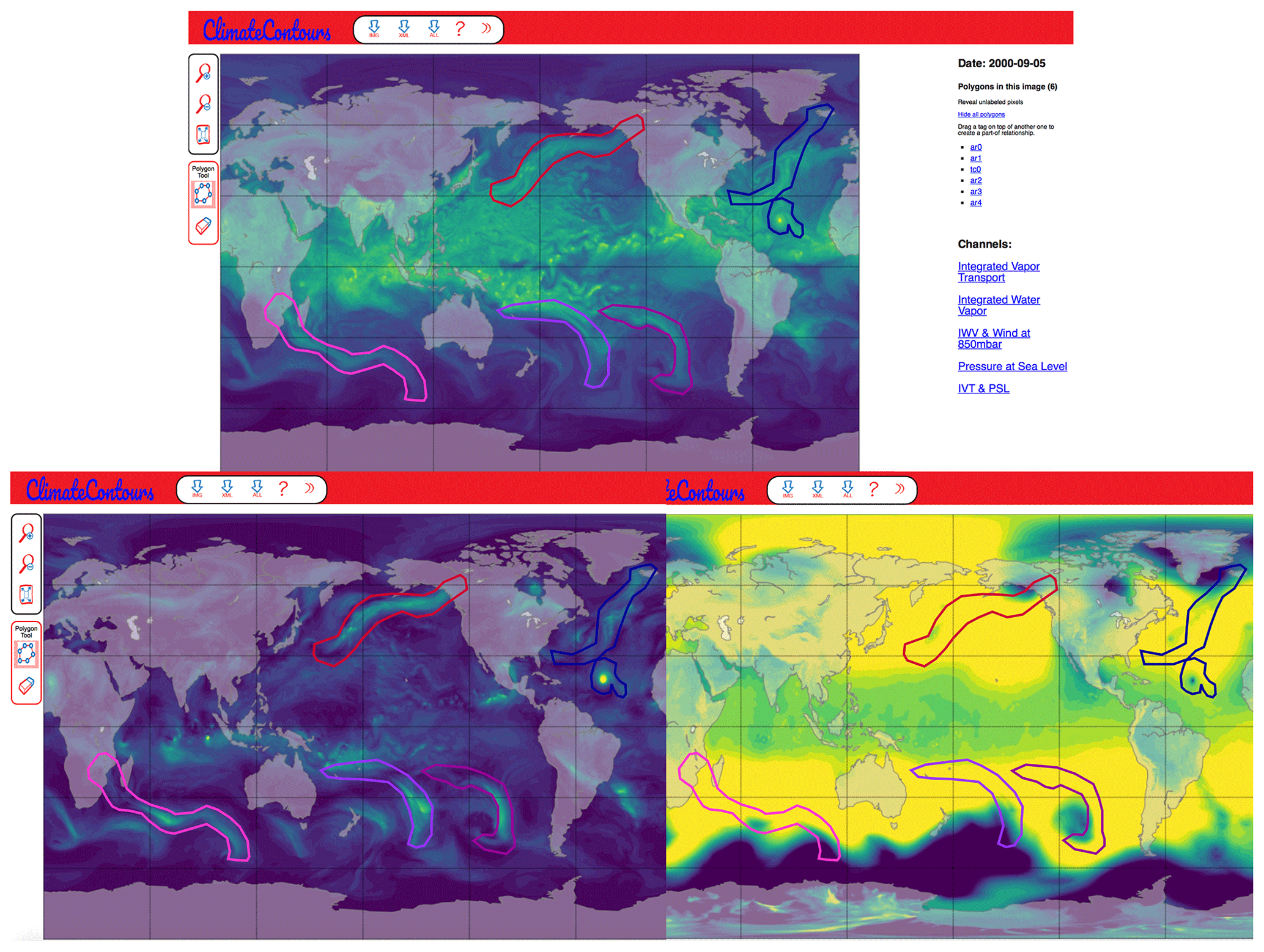
Figure 1 The ClimateContours web-based labeling interface. Labelers can choose different channels (physical variables) on the right side of the GUI to display different variables or combinations of variables on the global map. On top: integrated water vapor (IWV) is shown with labels of ARs and TCs; bottom left: integrated vapor transport (IVT); bottom right: pressure at sea level (PSL).

The labeler has the option to delete edges or the entire polygon and re-create polygons as many number of times as they wish. In addition, a labeler may zoom in to view events at a finer scale and switch between various views of raw and derived variables to help inform their labeling.

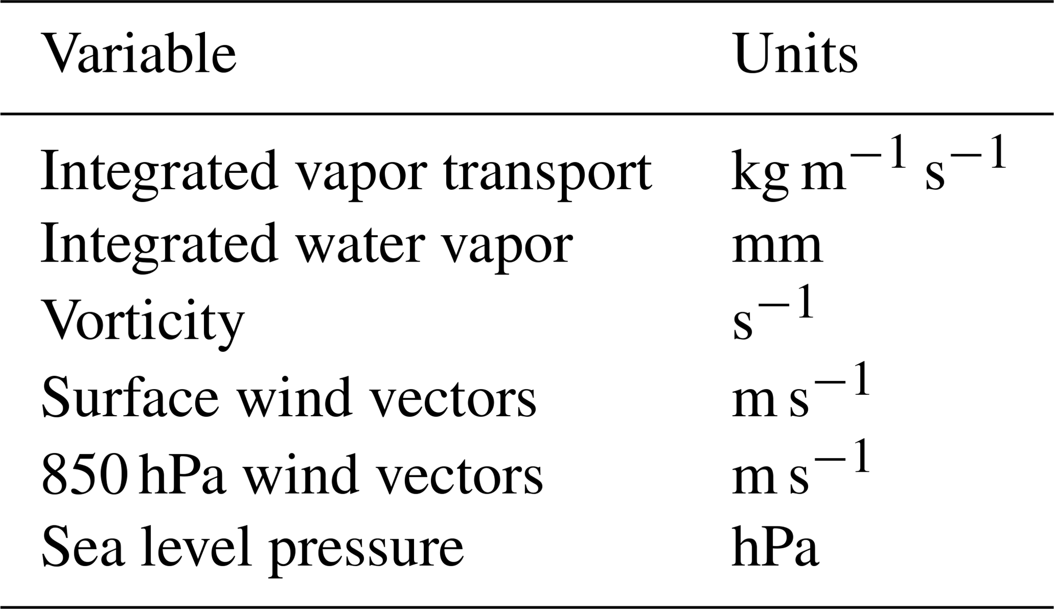
Currently, ClimateContours renders snapshots from 25 km Community Atmospheric Model (CAM5.1) output (Wehner et al., 2014). We choose this particular model for its high resolution, its high fidelity for simulating tropical cyclones and atmospheric rivers, and the large amount of readily available output data for multiple climate change scenarios, thus making training DL models and testing their generalization capabilities viable. Output from this model contains dozens of physical variables, such as wind velocity, temperature, pressure, and humidity at different vertical levels and across the globe (three spatial dimensions and time). These variables contain information relevant to the dynamics of weather and climate phenomena, but not all variables are needed to detect a weather event. Based on the experience and wealth of knowledge accumulated by meteorologists, and weather and climate scientists, and for relative ease of use, we provide a subset of six variables – in various combinations – to the user to aid them in creating labels for TCs and ARs through ClimateContours. These are the leading variables that are used to define and characterize TCs and ARs and are shown in Table 1.

Table 1 Variables for the definition and characterization of TCs and ARs.

2.2 Labeling campaigns

In order to capture the expertise of climate scientists in characterizing ARs and TCs, and to obtain sufficient data to train deep neural networks, we conducted multiple labeling campaigns across several institutions and events. These included campaigns at LBNL, UC Berkeley, NCAR, Scripps/UCSD, the 2019 ARTMIP Workshop, and the 2019 Climate Informatics Workshop. For each labeling campaign, participants were briefed on how to use the ClimateContours tool and provided some background on the specifics of ARs and TCs and how to label them effectively. Overall, approximately 80 weather and climate scientists participated in the campaigns and contributed several hundred labeled snapshots of climate data. The ClimateNet dataset currently contains over 1000 carefully curated data labeled by experts using the ClimateContours tool (see Sect. 2.4 for information about the quality control process). The labeling campaigns proved to be invaluable not only for generating high-quality labeled data but also for obtaining feedback on the ClimateContours tool itself, variables of interest, and how the labeling process could be improved.

2.3 Diversity of expert labels

Just as there exist a dozen different heuristics for detecting weather events such as atmospheric rivers, tropical cyclones, and extra-tropical cyclones (Shields et al., 2018; Walsh et al., 2010; Neu et al., 2013), we find differences in the labels provided by experts using the ClimateContours tool. This is perhaps not unexpected as different experts inherently conceptualize and identify weather events in slightly different ways. The labeling campaigns shed useful light on the diversity of labeling styles and implicit assumptions of different experts, as is seen in Fig. 2. Disagreements and disparities were most common on the exact spatial extents of individual storms, and less so on the presence or absence of the storm. Some experts disagreed on edge cases, such as incipient events or those that were dissipating. However, we note that the disagreements between human labels were less severe than differences noticed in dedicated heuristics-based event detection intercomparison projects such as ARTMIP, TCMIP, and IMILAST, which exhibit significant disparities in the presence or absence of labeled extreme events and their boundaries (Shields et al., 2018; Wehner et al., 2018; Ullrich and Zarzycki, 2017; Neu et al., 2013; Walsh et al., 2010).

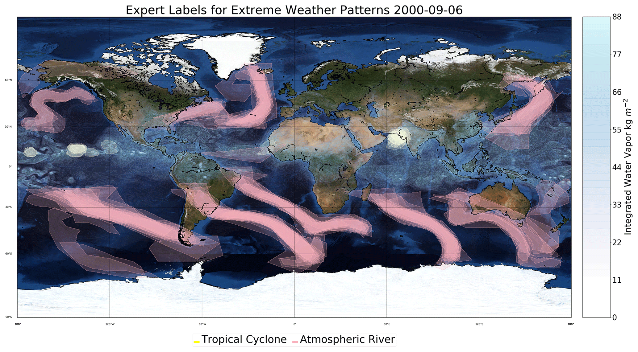
Figure 2 Comparison of 15 different expert labelings. Density of pink masks shows overlap of AR labels; density of white/yellow masks shows overlap of TC labels. The “bluemarble” map in the background included via Matplotlib's Basemap library is © NASA.

In Fig. 2, labels from 15 different experts are shown. Most experts agree on some of the prominent ARs and TCs, albeit with some variance in the precise boundaries. The two ARs in the South Atlantic Ocean and the TC off the west coast of India are examples of strong expert agreement. However, there are also quite a few discrepancies. A few labelers considered there to be ARs off the east coast of Australia, while most did not consider these patterns to represent ARs. Some of the smaller cyclonic structures in the equatorial Pacific also demonstrate discrepancies. One egregious error in labeling can be seen from the triangular AR polygon sitting on the Equator in the Atlantic, which was removed in the quality assurance and quality control (QA/QC) curation process.

2.4 Quality assurance and quality control

Any manual labeling campaign, even one conducted amongst experts, is subject to errors stemming from various sources: human errors (lack of expertise/understanding, lack of motivation/thoroughness, misinterpretation of instructions, mislabeled events, missed events, and fatigue) and technical errors (glitches in the web interface and infrastructure). It is simply unrealistic for us to expect that all images will be labeled to a consistently high degree of accuracy. In order to address this important issue, we formed a small team of QA/QC experts from the co-author list on this paper. The experts had a background in both climate and computer science, had a good working knowledge of TC and AR patterns, and were briefed on and motivated to reach a high target accuracy for the labeled dataset. This core team manually examined and executed a thorough QA/QC process on about 500 samples to correct for errors.

The top priority for the QA/QC team was to fix mislabeled and missed events. A second type of QA/QC task was to modify the boundaries of correctly labeled events based on an internal consensus grounded in the basic defining characteristics, such as the following: (i) TCs exist in the tropics and are sufficiently intense, measured by low sea level pressure and high vorticity; (ii) ARs sometimes are associated with ETCs, but the ETCs should not be included in the AR boundary; and (iii) slight differences exist in AR signatures in integrated water vapor (IWV) and integrated vapor transport (IVT) fields, and we choose boundaries based on geometric criteria, i.e., that “ARs are long, narrow, and transient corridors of strong horizontal water vapor transport …” (the American Meteorological Association's definition of AR; http://glossary.ametsoc.org/wiki/Atmospheric_river, last access: 14 December 2020).

Despite making such QA/QC adjustments to experts' labels, there remained some variety amongst AR and TC labels, perhaps representative of the lack of a clear theoretical and quantitative definition for these events. We argue that these relatively minor differences are not a detriment to the training and evaluation of the DL model, as will be shown in the Results section.

3 Methods

3.1 Deep learning for segmentation

In this section, we present our deep learning approach to generate high-quality segmentation masks (i.e., separating objects of interest from the background) for ARs and TCs, using the curated ClimateNet dataset. We model this problem as a semantic segmentation task; i.e., the goal is to assign a class label to every pixel for a given input image. In our case, the input image is the CAM5.1 25 km grid comprising atmospheric fields, and the output class labels are TC, AR, and background (BG).

3.1.1 Model

Figure 3 DeepLabv3+ network: all convolutional layers are followed by a batch normalization and a rectified linear unit (ReLU) activation layer, which are omitted from this schematic for the sake of brevity. “Sep. Conv” denotes depth-wise separable convolution. The pooling module consists of a two-dimensional pooling layer, followed by a convolutional layer, a batch normalization layer, and a ReLU activation layer. For more details, we refer the reader to Chen et al. (2018).

The deep neural network architecture used in this work is the DeepLabv3+ architecture (see Fig. 3) developed by Chen et al. (2018) based off of Chollet (2016). This architecture has attained state-of-the-art results across various semantic segmentation benchmarks in the computer vision community (PASCAL VOC 2012 and Cityscapes). In order to map from our input (four-channel climate data) to the segmentation mask that corresponds to it, DeepLabv3+ extracts pixel-wise segmentation scores. A pixel then gets assigned to the highest scoring class. DeepLabv3+ consists of an encoder which captures rich semantic information across multiple scales. The idea of an encoder is a series of learned, hierarchical filters that extracts useful information as pertaining to the task defined – in this case, segmenting ARs and TCs from background. The decoder module then up-samples or, in other words, goes from a lower to higher resolution to produce refined object boundaries. There are learnable weights associated with both the encoder and the decoder which are learned together while trying to minimize the loss. The loss for the network we use is the cross-entropy between the predicted masks and the ground truth labels for a given input.

We use a PyTorch implementation of DeepLabv3+ (https://github.com/MLearing/Pytorch-DeepLab-v3-plus, last access: 14 December 2020). The input to the model consists of an array of size $(\mathrm{4},\mathrm{1152},\mathrm{768})$. It contains atmospheric data from four different channels; namely TMQ (total vertically integrated precipitable water), U850 (zonal wind at 850 mbar pressure surface), V850 (meridional wind at 850 mbar pressure surface), and PRECT (total convective and large-scale precipitation rate). The output, as discussed earlier, is a segmentation mask of size (1152,768), where each element in the mask takes the value of 0 (BG), 1 (TC), or 2 (AR).

3.1.2 Training

We study the learning capabilities of DeepLabv3+ on datasets D₁ and D₂, which correspond to two CAM5.1 scenarios – (i) All-hist and (ii) the so-called UNHAPPI (Wehner et al., 2018; Mitchell et al., 2017; Wehner et al., 2014). The All-hist scenario runs from 1995 to 2015 and includes all natural and anthropogenic forcings. The Half a degree Additional warming, Prognosis and Projected Impacts (HAPPI) experimental protocol was designed to compare the effects of stabilizing anthropogenic global warming at 1.5 and 2.0 ^∘C over preindustrial levels (Mitchell et al., 2017). The UNHAPPI scenario a stabilizes the anthropogenic warming at 3 ^∘C over preindustrial levels. The details of both scenarios can be found in the listed papers.

Dataset D₁ consists of 128 000 samples; each sample conforms to the input format described above. Every sample in this dataset has TCs and ARs detected via heuristics (Prabhat et al., 2015a; O'Brien et al., 2020). For training, we split D₁ into a training set, which is a randomly sampled subset that contains 51 200 samples (40 % of all samples in D₁), and validation and test sets, which are disjoint sets each randomly sampled from the remaining 60 %. This provides a heuristics-based baseline, against which we compare the DL model trained on the ClimateNet dataset.

To create the human-expert-labeled ClimateNet dataset, we sampled 219 unique images from D₁ and used them for labeling campaigns. Each image is labeled by at least one human expert; that is, there also exist samples which are labeled by multiple experts. A total of 459 images were acquired upon the completion of the labeling campaigns. The training set for ClimateNet dataset $D_{\mathrm{1}}^{*}$ contains 422 (92 %) samples; validation and test sets contain 18 (4 %) and 19 (4 %) samples, respectively.

A unique challenge in applying standard computer-vision-based DL architectures to climate problems is that climate images are heavily imbalanced: 94 % of the pixels in ClimateNet data correspond to the “background” class. The DL architecture can naively learn a mapping of any input image pixel to the background class, and be correct 94 % of the time! In order to account for this unique challenge, we train our network by optimizing the weighted cross-entropy loss function using the Adam optimizer (Kingma and Ba, 2014). For such a loss, the class weights are usually defined to be the inverses of class frequencies. However, this choice for the class weights leads to certain numerical issues (Kurth et al., 2018). In order to circumvent these issues, we use the squared inverses of class frequencies as class weights.

We use a learning rate scheduler that multiplicatively reduces the learning rate each time the performance on the validation set does not improve for three epochs in a row and set the initial learning rate to be $\mathrm{1.5}\times {\mathrm{10}}^{-\mathrm{3}}$. We distribute the training process over eight GPUs and use a batch size of 16. For both datasets, we initialize the model with random weights and stop the training as soon as the model's performance on the validation set starts degrading. This corresponds to a training time of 20 epochs for dataset D₁ and 5 epochs for dataset $D_{\mathrm{1}}^{*}$.

During training, we track the loss incurred by the model on the training and validation sets. We note that, while the model did begin to incur larger losses on the validation set, the incurred training loss never converged. From this observation, we conclude that the model has potential to learn the segmentation masks even better if provided with more hand-labeled data.

3.2 Inference

Once the training phase is over, we obtain model M₁, which was trained on D₁, and model $M_{\mathrm{1}}^{*}$, which was trained on $D_{\mathrm{1}}^{*}$, and run inference on held-out samples from the same dataset. We also use the models M₁ and $M_{\mathrm{1}}^{*}$ to run inference on a completely different dataset, D₂, which corresponds to a climate change scenario. We used a single GPU for this process as inference is computationally much more lightweight than training. As described above, the models produce segmentation masks of size (1152,768) for every sample in their respective test sets. These masks are then used to evaluate the performance of the model. A detailed discussion of the results is reported in Sect. 4.2.

3.3 Conditional precipitation analyses

Once deep learning has been applied to obtain pixel-level segmentation masks for TCs and ARs, a host of downstream analytics can now be conducted; for example, we can extract and summarize various conditional probability distributions associated with individual event types. In this paper we report on global precipitation associated with TCs and ARs and regional precipitation associated with ARs in the state of California, and TCs in the Gulf of Mexico. Further, we present percentiles and scaling relationships due to global warming of extreme precipitation associated with TCs and ARs at global and regional scales.

A key challenge in conducting such highly precise analytics is the requirement to create conditional probability distributions over O(10M)–O(10)B pixels, where each pixel contains the value of a physical quantity at a grid point in the climate model output. We leverage the fastKDE package, developed by O’Brien et al. (2014, 2016), to compute these distributions efficiently and effectively in seconds to minutes on a single workstation.

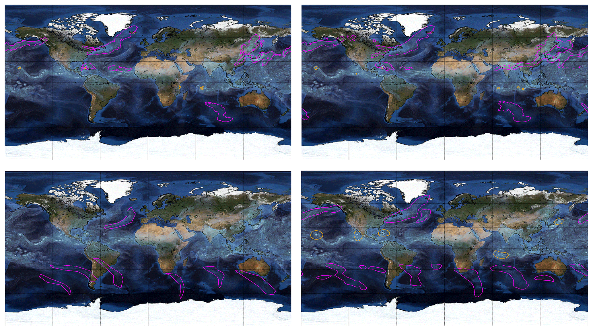
Figure 4 Comparison of labels from TECA (top left), model predictions trained on TECA (top right), the ClimateNet dataset (bottom left), and model predictions trained on ClimateNet (bottom right). The “bluemarble” map in the background included via Matplotlib's Basemap library is © NASA.

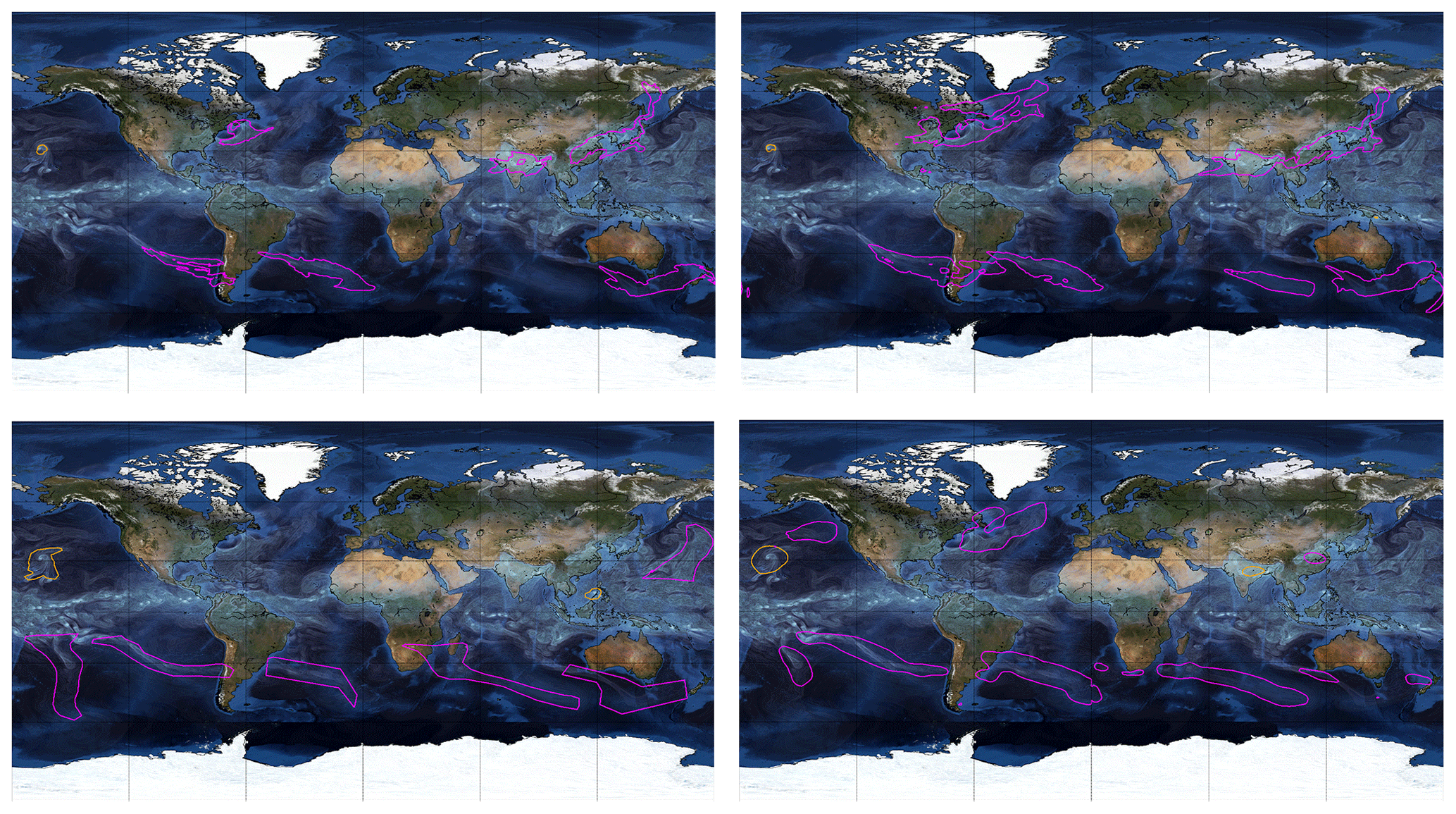
Figure 5 Comparison of labels from TECA (top left), model predictions trained on TECA (top right), the ClimateNet dataset (bottom left), and model predictions trained on ClimateNet (bottom right). The “bluemarble” map in the background included via Matplotlib’s Basemap library is © NASA.

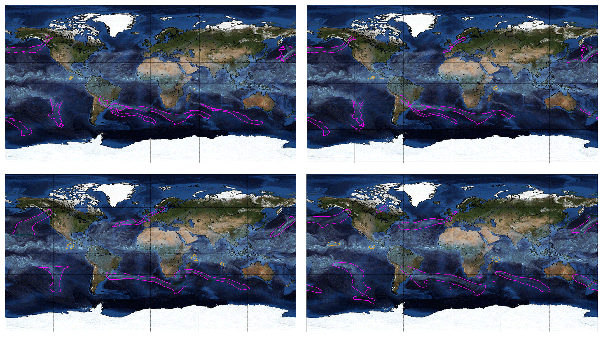
Figure 6 Comparison of labels from TECA (top left), model predictions trained on TECA (top right), the ClimateNet dataset (bottom left), and model predictions trained on ClimateNet (bottom right). The “bluemarble” map in the background included via Matplotlib’s Basemap library is © NASA.

4 Results

4.1 ClimateNet dataset

The curated expert-labeled ClimateNet dataset, the trained DL segmentation model, and the PyTorch code to use the model in inference mode are available for download at https://portal.nersc.gov/project/ClimateNet/ (last access: 14 December 2020).

4.2 Segmentation results

4.2.1 Qualitative assessment

We compare visually the performance of the DL model M₁ trained on heuristics and $M_{\mathrm{1}}^{*}$ trained on human expert labels in Figs. 4, 5, and 6. These images illustrate that (i) DL models are effective at learning mappings between input images and output pixel masks that exist in the training data (i.e., they faithfully emulate the data they are trained on); (ii) although the weather and climate communities have thoughtfully developed heuristic algorithms to label TCs and ARs, carefully curated human expert labels seem to be more reliable at capturing both presence or absence of events and their spatial extents; (iii) the DL model trained on human expert labels from ClimateNet, $M_{\mathrm{1}}^{*}$, performs better at segmenting TCs and ARs compared to the DL model trained on heuristic labels, M₁; and (iv) the DL model $M_{\mathrm{1}}^{*}$ predicts high-quality segmentation masks for TCs and ARs that are temporally consistent, even though the notion of temporal persistence of TCs and ARs is not incorporated into the training process. We encourage readers to examine rendered movies at https://tinyurl.com/unhappi-yt (last access: 14 December 2020), which showcase the realism and temporal stability of the segmented TCs and ARs. While there are a few false positives and false-negative events, all strong TCs and ARs are successfully detected, segmented, and tracked by the DL model $M_{\mathrm{1}}^{*}$.

4.2.2 Quantitative assessment

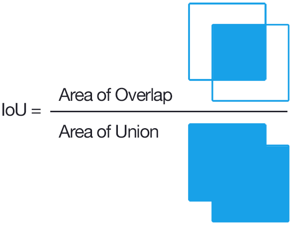
Figure 7 Schematic that shows IoU of two square masks. IoU is defined as the ratio of “the area of the intersection of two segmentation masks” to “the area of their union”. Note that for the two squares shown here even an 80 % overlap of their edges results in an IoU of 0.47, because the intersection area is 0.64 units and the union is 1.36 units. Source: https://www.pyimagesearch.com/2016/11/07/intersection-over-union-iou-for-object-detection/ (last access: 14 December 2020).

We measure the performance of our model using the mean intersection-over-union (IoU) metric. Given two binary segmentation masks the IoU is defined as the ratio of the area of the intersection of two segmentation masks to the area of their union, as illustrated in Fig. 7. While it is a measure of the agreement between two masks, it can be far from unity, especially for masks that are small in size because small disagreements in their overlap are amplified by this measure. Hence we emphasize that IoU not be confused with accuracy. Nevertheless, it is a useful metric for evaluating how well a DL model emulates the characteristics of the data it is trained on. Since we have multiple classes in our study, we calculate a mean IoU metric as the mean of the IoUs of the three classes, i.e., AR, TC, and background.

Table 2 Model M₁ achieves IoU scores similar to those reported in Kurth et al. (2018). After training on ClimateNet, model $M_{\mathrm{1}}^{*}$ performs similar to human experts. The overall mean IoU is limited by the TC IoU.

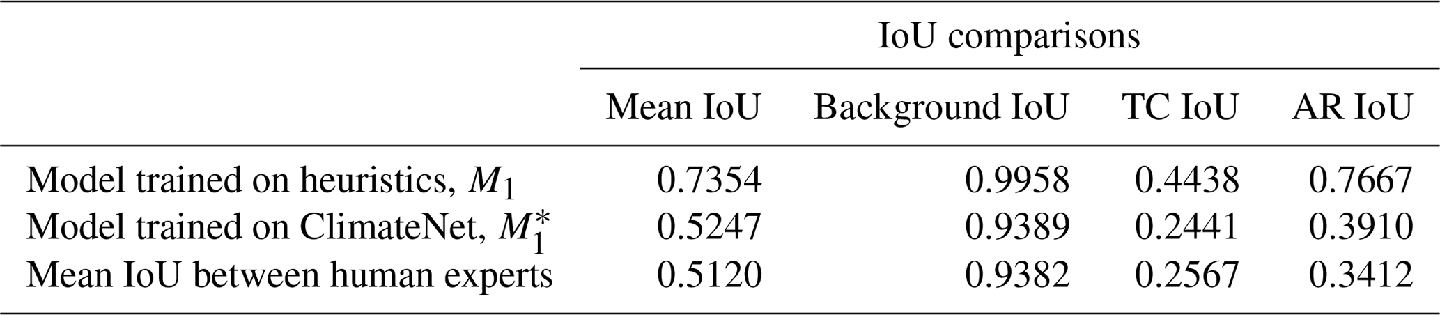
Table 2 shows comparisons of IoUs obtained for the DL model (DeepLabv3+) trained on labels from heuristics (first row), labels from human experts (second row), and between human experts (third row). In the first and the second row the IoU is calculated on a “held-out” test set that has not been seen by the model during training or validation. For model M₁, the IoU is calculated between the model predictions and the heuristic labels; in this case each image has only one set of heuristic labels (from Toolkit for Extreme Climate Analysis (TECA) and TECA Bayesian AR Detector (TECA-BARD)). For model $M_{\mathrm{1}}^{*}$, the IoU is calculated between the model predictions and every human expert label that exists for that image (note that the number of human expert labels is not the same for each image), and then averaged. In the third row we calculate, pair-wise, the IoU between every pair of human expert labels for a given image and then average over all images. The third row gives a measure of how well any two experts agree on their labels, and we use this as the target metric that the DL model M₂ aims to achieve; i.e., we train the model to perform similarly to a human expert.

Given clear, deterministic ground truth labels, where the exact boundaries of every event of each class are well defined and not subject to discrepancies or uncertainties, the mean IoU is a useful quantitative metric for assessing the quality of segmentation techniques. In our context, however, because the boundaries of ARs and TCs can be hard to define exactly with certainty, it is useful to compare human experts against each other to obtain a measure of the mean IoU between any two human experts, before evaluating performance of the deep learning model against human experts.

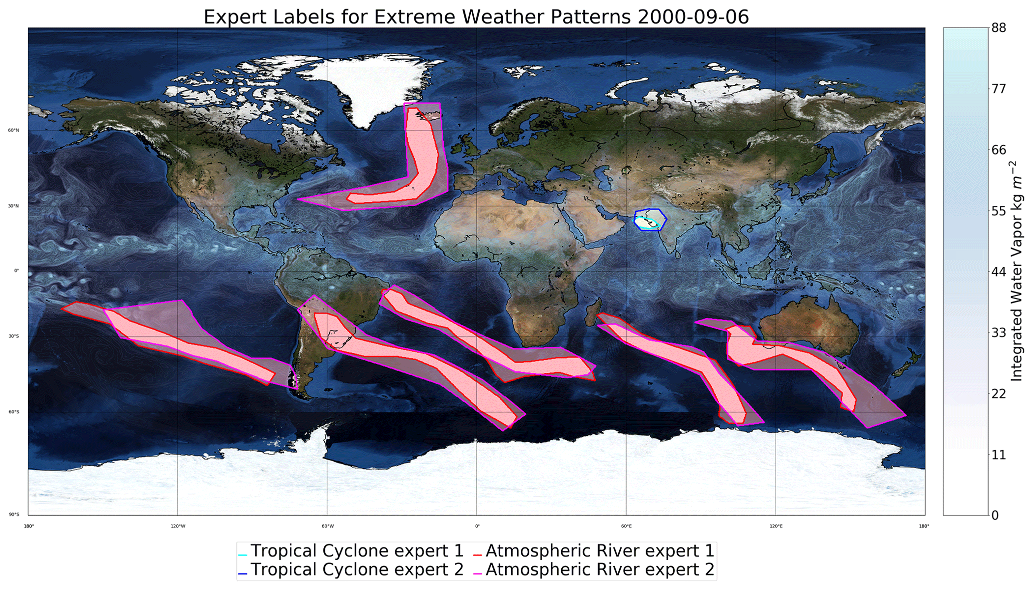
Figure 8 Comparison of two different expert labelings with an IoU of 0.59. Note that – even though, visually, the experts appear to agree to a large extent on their labels of AR and TC events in this snapshot – the quantitative IoU metric is only 0.59. Hence we emphasize that IoU not be confused with accuracy; good agreement even amongst expert labelers can result in IoU values far from unity. A perfect match (i.e., IoU = 1) only results when two labelers agree on every single pixel of the image. As is apparent from this figure, even relatively minor differences in the labels for TCs can disproportionately impact the mean IoU. The “bluemarble” map in the background included via Matplotlib's Basemap library is © NASA.

In Fig. 8 we show an example of the comparison between two human experts for one snapshot. The background class is most dominant because TCs and ARs occupy a small fraction of the total number of pixels on any given image; hence IoUs for background tend to be quite high, as seen in Table 2. However, for TCs and ARs, the IoU can drop to significantly lower values because minor differences in event boundaries for small events can result in low IoU values, as illustrated in Fig. 7. Even though the experts appear to agree reasonably on their event labels and masks, the mean IoU for these two human experts is 0.59. These results are comparable to those reported in Kurth et al. (2018).

4.3 Conditional precipitation results

One of the main implications of pixel-wise segmentation for climate science is the ability to conduct highly precise analyses conditional on event types, for example, one could ask the question, “how might extreme precipitation due to land-falling atmospheric rivers change in California due to climate change?” Here we show some examples of such analyses using precipitation data using the segmentation masks from model $M_{\mathrm{1}}^{*}$ trained on human expert labels (the ClimateNet dataset).

4.3.1 Global tropical cyclone precipitation

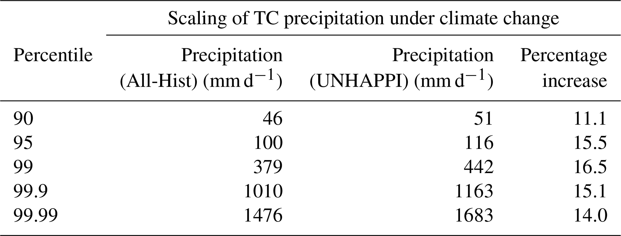
First we calculate annual precipitation from tropical cyclones across the globe for both climate scenarios, All-Hist and the so-called UNHAPPI scenario, by extracting precipitation at every pixel within TC segmentation masks from all data points (50 years of data from All-Hist and UNHAPPI). We note that these are average daily rain rates for a 25 km model at 3-hourly time steps. Figure 9 shows how tropical cyclone precipitation intensifies and increases in a warmer world. In line with previous studies (Wehner et al., 2018), we see that the probability density function (PDF) of TC precipitation shifts to higher rain rates under global warming. In Table 3 we show the percentiles and rain rates for extreme precipitation from TCs (annual and global). We compare the actual scaling of extreme precipitation with the Clausius–Clapeyron (CC) scaling rate of 7 % per degree Kelvin, the scaling rate of available precipitable water in highly saturated atmospheres (O'Gorman and Schneider, 2009; Pall et al., 2007; Allen and Ingram, 2002). Notably, these studies found that global mean precipitation increases tend to be lower than the increases in the extremes due to different controlling physical mechanisms for each. The tropical (40^∘ S–40^∘ N) mean sea surface temperature (SST) increase between All-Hist and UNHAPPI is 1.6 K. If extreme tropical cyclone precipitation were to follow a CC scaling relationship, we would expect about an 11.2 % increase in extreme precipitation in the warmer simulation. In the last column of Table 3 we see that extremes at the 95th percentile and above scale at super-CC rates. These findings are consistent with extreme hurricane event attribution studies (Risser and Wehner, 2017; Patricola and Wehner, 2018; van Oldenborgh et al., 2017; Wang et al., 2018) and other idealized tropical analyses (O'Gorman and Schneider, 2009).

Figure 9 Conditional PDF for tropical cyclone precipitation computed using fastKDE (O’Brien et al., 2016).

Table 3 Scaling relationships for global tropical cyclone precipitation at various percentiles for extremes. The tropical (40^∘ S–40^∘ N) mean SST increases by 1.6 K from 297.4 K (All-Hist) to 299.0 K (UNHAPPI). CC scaling for this temperature increase would be 11.2 %. Note that extreme precipitation at the 95th percentile and higher exceeds CC scaling with increases about 15 %.

4.3.2 Global atmospheric river precipitation

Here we present annual precipitation from atmospheric rivers across the globe for both climate scenarios, All-Hist and UNHAPPI. Figure 10 shows how AR precipitation intensifies and increases in a warmer world. In line with previous studies (Warner et al., 2015; Espinoza et al., 2018; Gershunov et al., 2019; Gao et al., 2015), we see that the PDF of AR precipitation shifts to higher rain rates.

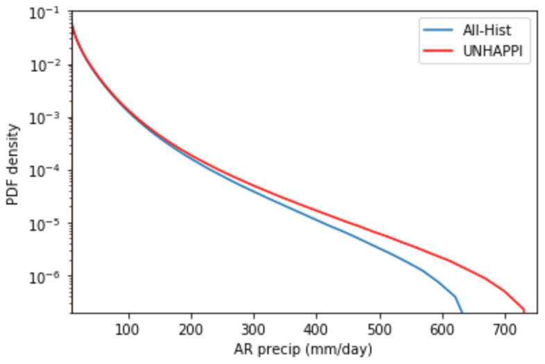
Figure 10 Conditional PDF for atmospheric river precipitation computed using fastKDE (O’Brien et al., 2016).

Table 4 Scaling relationships for atmospheric river precipitation at various percentiles for extremes. Note that extreme ARs have more extreme precipitation in a warmer world. The mean SST for regions where ARs are most dominant (mid-latitudes, i.e., 30–60^∘ S and 30–60^∘ N) increases by 1.7 K from 284.9 K (All-Hist) to 286.6 K (UNHAPPI). Hence CC scaling implies a 11.9 % increase in precipitation.

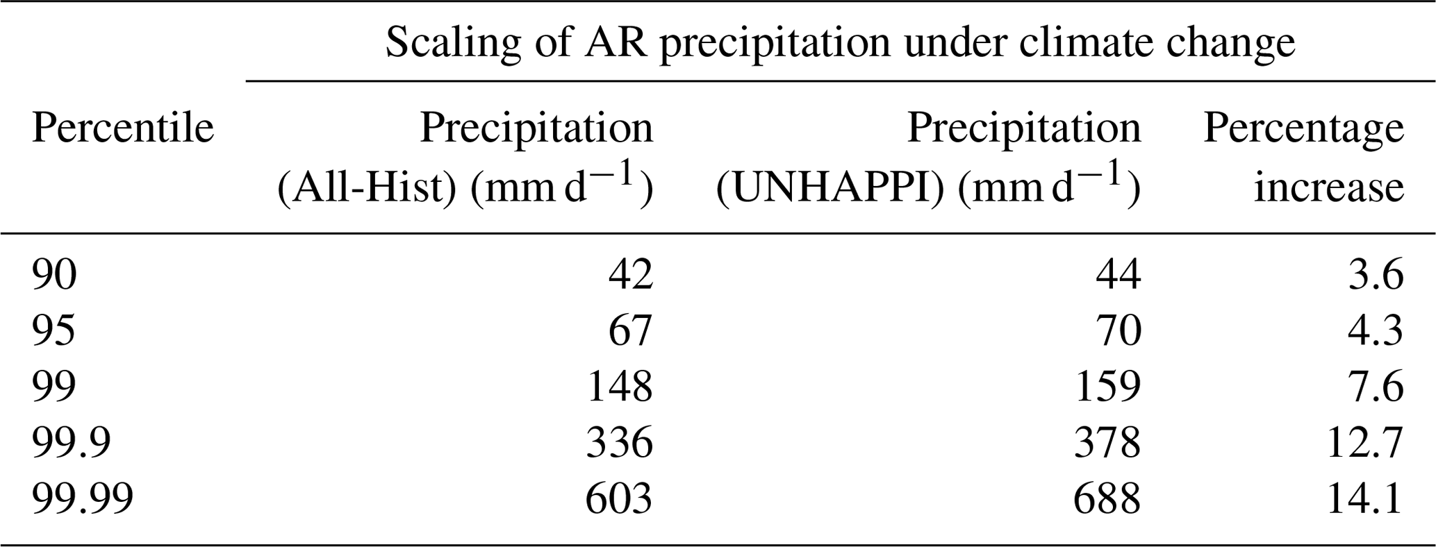
In Table 4 we show the percentiles and rain rates for extreme precipitation from ARs (annual and global). The mean SST for AR zones (mid-latitudes, i.e., 30–60^∘ S and 30–60^∘ N) increases from 284.9 K (All-Hist) to 286.6 K (UNHAPPI). Hence, for this 1.7 K increase in the reference temperature for ARs, CC scaling implies an 11.9 % increase in precipitation. The actual percentage increases are shown in the last column, and we see that AR precipitation increases scale less than CC for UNHAPPI vs. All-Hist below the 99th percentile, but more than CC for the most extreme events (at and above the 99th percentile). Gao et al. (2015) found projected increases in precipitation from ARs are primarily due to thermodynamic effects controlled by CC, while dynamical effects work counter to this increase for North America. Furthermore, as can be seen in the monotonic increase in scaling percentages across percentiles, precipitation in stronger ARs intensifies more than weaker ARs in a warmer world (compared to All-Hist). For comparison, Warner et al. (2015) saw mean winter precipitation increase by 11–18 % for the west coast of North America under RCP8.5, while for extreme IVT days, which are closely associated with ARs in this region, precipitation increases by 15–39 %. The findings here are consistent with Warner et al. (2015), although our reported percentages are lower, potentially due to Warner et al. (2015) examining wintertime precipitation in California, which shows robust projected increases (Swain et al., 2018), whereas we examine across the entire year globally.

We now address two questions that highlight the power of pixel-wise segmentation in making localized, precise statements about tropical cyclones and atmospheric rivers in the USA.

4.3.3 Tropical cyclone precipitation in Gulf of Mexico

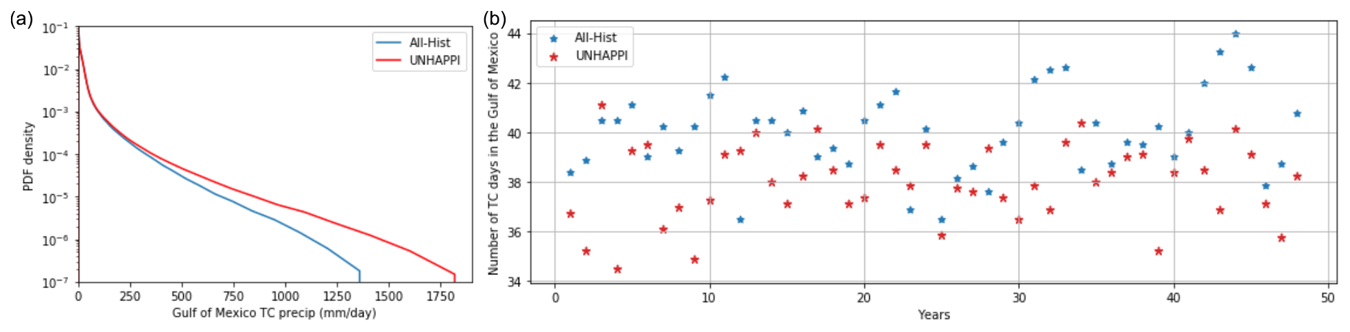
Figure 11 (a) Conditional PDF for tropical cyclone precipitation in the Gulf of Mexico using fastKDE (O’Brien et al., 2016); (b) number of tropical cyclone days annually in the Gulf of Mexico, shown for 50 years of All-Hist and UNHAPPI.

Table 5 Scaling relationships for extreme TC precipitation at various percentiles in the Gulf of Mexico. The increase in mean SSTs in the Gulf of Mexico between All-Hist (299.5 K) and UNHAPPI (301.3 K) is 1.8 K, which results in a CC scaling of 12.6 %. We see that extreme precipitation here scales well above CC scaling, corroborated by other studies (Risser and Wehner, 2017; van Oldenborgh et al., 2017; Wang et al., 2018).

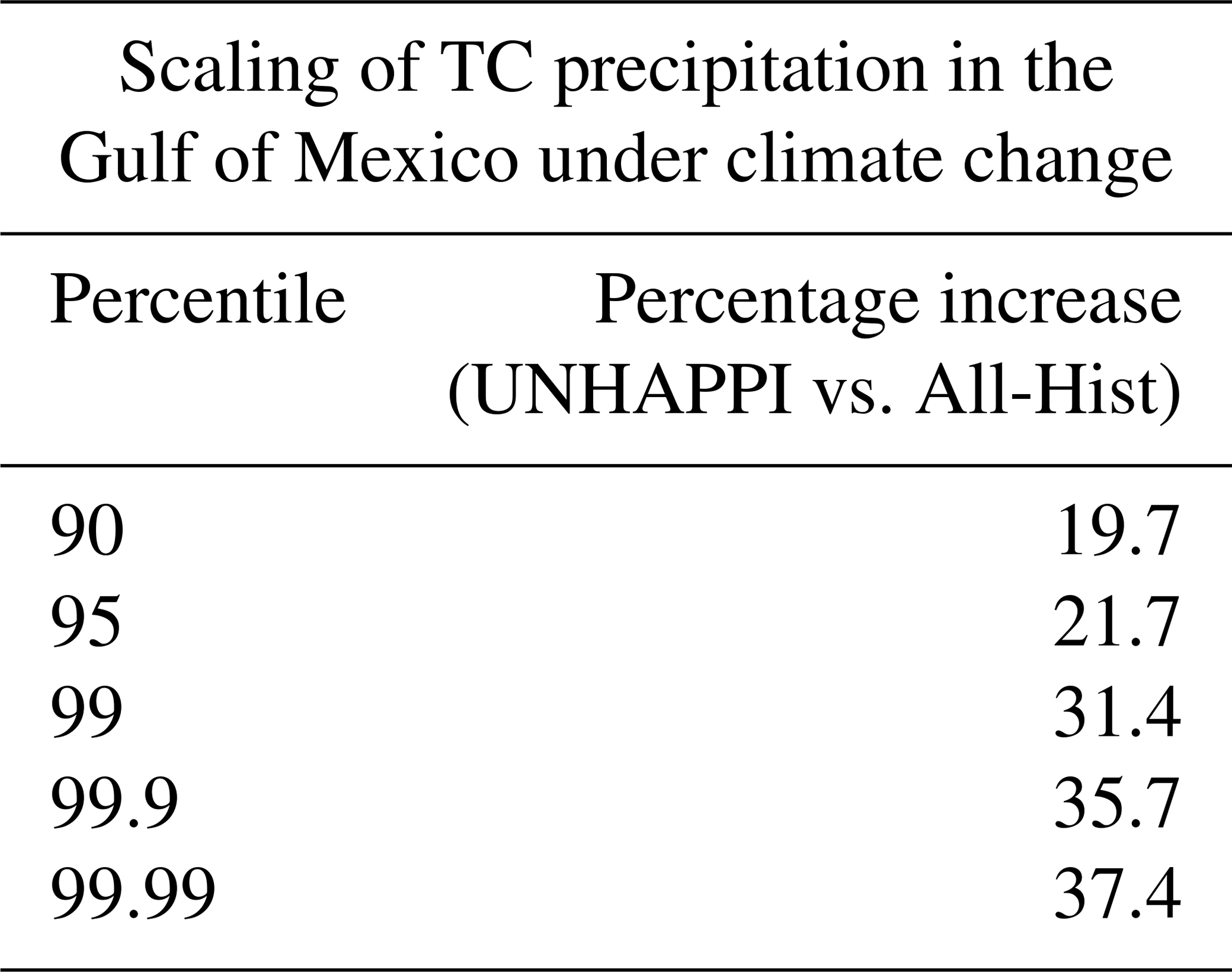
First, we focus on the Gulf of Mexico and examine how TC precipitation changes in this region due to global warming. Once again, we calculate the PDFs of precipitation and changes in percentiles of extreme precipitation. The percentage increase in extreme precipitation corresponding to different percentiles is shown in Table 5. The increase in the Gulf of Mexico's temperature between All-Hist (299.5 K) and UNHAPPI (301.3 K) is 1.8 K, which corresponds to a CC scaling of 12.6 %. The last column of this table shows that extreme precipitation due to TCs in the Gulf of Mexico scales well above CC, up to almost 3 times the CC scaling for the most extreme events. Table 5 also suggests that extreme Atlantic hurricanes that are formed in or enter the Gulf of Mexico rain much more intensely compared to global TC trends (illustrated in Fig. 9). Further, we examine the number of TC days (defined as a day when at least one TC is active within the specified region, here the Gulf of Mexico) in both climate scenarios. In line with what is expected for Atlantic hurricanes under global warming (Wehner et al., 2018; Knutson et al., 2019), we find that, on average, the number of TC days per year decreases from 40.1 (All-Hist) to 37.7 (UNHAPPI). Hence, total precipitation increases by 18.8 % per TC day, suggesting that the fewer TCs in the warmer UNHAPPI simulations produce much more precipitation than the cooler All-Hist.

4.3.4 Atmospheric river precipitation in California

Next we focus on California and examine how AR precipitation changes in this region due to global warming. We choose California as ARs play a critical role in California; they can deliver 50 % of the annual precipitation but also be a threat to public safety and infrastructure through extreme events (Dettinger et al., 2011).

Figure 12 (a) Conditional PDF of atmospheric river precipitation in California using fastKDE (O’Brien et al., 2016); (b) number of atmospheric river days annually in California, shown for 50 years of All-Hist and UNHAPPI.

Table 6 Scaling relationships for extreme AR precipitation at various percentiles in California. The increase in SST off the coast of California between All-Hist and UNHAPPI is 1.3 K, which corresponds to a CC scaling of 9.1 %. Note that extreme precipitation scales at super-CC rates.

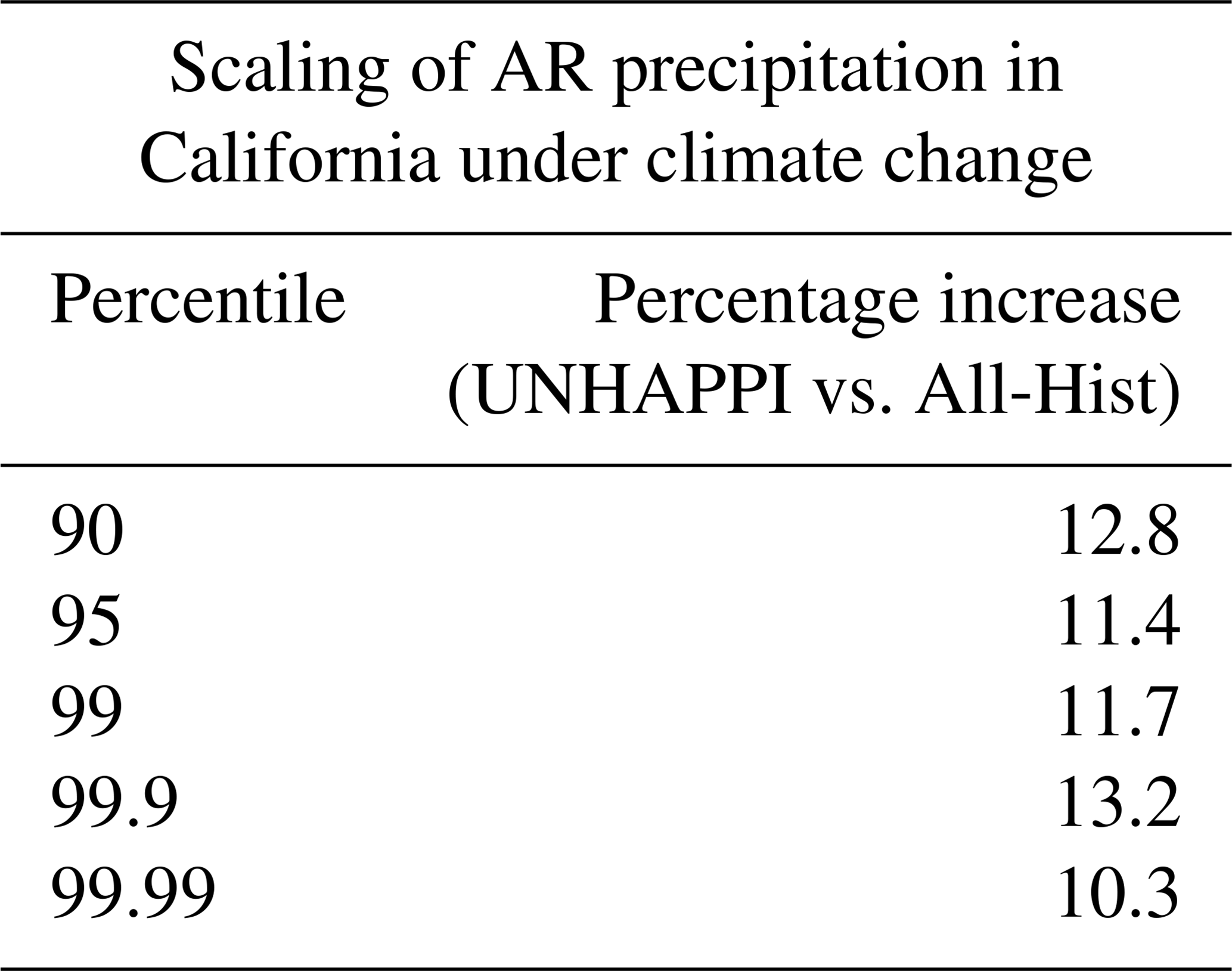
Once again, we calculate the PDFs of precipitation and changes in percentiles of extreme precipitation. The percentage increase in extreme precipitation corresponding to different percentiles is shown in Table 6. The increase in SST off the coast of California between All-Hist (288.4 K) and UNHAPPI (289.7 K) is 1.3 K, corresponding to CC scaling of 9.1 %. Note that for all percentiles presented in Table 6, we observe super-CC scaling of extreme precipitation from California ARs. These findings are similar to those of Gao et al. (2015) and Warner et al. (2015).

We also examine the number of AR days (defined as a day when at least one AR is active within the specified region, here California) in both climate scenarios. We find that, on average, the number of AR days per year increases from 36.1 (All-Hist) to 37.9 (UNHAPPI). However, total precipitation increases by 36.9 % per AR day, suggesting that west coast ARs tend to produce much more precipitation in UNHAPPI. These findings are consistent with a global analysis of ARs under climate change by Espinoza et al. (2018) and regional analysis by Swain et al. (2018). Swain et al. (2018) found projected increases in California's extreme precipitation event frequency. Furthermore, they found these increases to occur during the core winter months and decrease outside of these months. Espinoza et al. (2018) found fewer individual AR events under climate change but an increase in AR conditions globally. Both Espinoza et al. (2018) and Massoud et al. (2019) report AR conditions to increase by 50 % and AR IVT strength to increase by 25 %. This growth in AR conditions is linked to the increase in both size and IVT intensity of individual AR events. The change in AR days found here falls below the 50 % reported by Espinoza et al. (2018) and Massoud et al. (2019) as their AR condition frequency calculations were done at a grid level which is relatively more sensitive to the increased length and width of ARs compared to our metric. Regardless of AR strength or size, if it makes contact with California, it will register as an AR day.

5 Conclusions and future work

We have demonstrated conclusively that deep learning models trained on curated expert-labeled climate data – using ClimateNet – are powerful tools for segmenting extreme weather patterns in climate datasets, enabling precision climate data analytics. We have developed an end-to-end infrastructure for acquiring expert-labeled data (via ClimateContours); curating the data carefully (using rigorous QA/QC protocols); training DL segmentation models; running DL segmentation models in inference mode; and conducting downstream conditional precipitation analyses.

The proposed dataset – ClimateNet – and end-to-end infrastructure provide several unique capabilities: (i) it enables us to perform fine-grained, highly precise data analytics, such as examining changes in frequency and intensity of weather patterns at specific geographic locations across the globe; (ii) it can be applied to different climate scenarios and different datasets without tuning since it does not rely on threshold conditions unlike heuristic algorithms currently used in the community; and (iii) the method is suitable for rapidly analyzing large amounts of climate model output. Further, the method can likely be used directly with reanalysis products or observational data using transfer learning, as shown successfully for a similar DL-based method by Ham et al. (2019). While we do not explicitly test the transferability of this model to observations and reanalysis products, we intend to pursue this in future work.

Our work highlights the advantages of transitioning to modern, data-driven DL methods for high-precision climate data analytics. While our preliminary results are promising, we highlight current limitations in our methodology and identify opportunities for future studies:

1. Limited training data: The quality of our segmentation results is fundamentally limited by access to large amounts of expert-labeled data. We have only been able to curate ≈ 500 expert-labeled images thus far, and while the resulting DL model performs reasonably on held-out datasets, we expect that the performance will be improved further with larger amounts of curated expert-labeled data. We appeal to the climate science community to contribute labels to the ClimateNet project – an open-source, community project – which is live and freely usable by anyone worldwide at https://www.nersc.gov/research-and-development/data-analytics/big-data-center/climatenet/ (last access: 14 December 2020).

   • Applicability of transfer learning: We intended to leverage the relatively large amount of training data available via AR and TC pattern detection heuristics, such as TECA (Prabhat et al., 2015a), and a smaller amount of ClimateNet labeled data via transfer learning (Zamir et al., 2018) to train a model first on heuristics-based training samples followed by “fine tuning” using ClimateNet data. This approach, however, produced a model that was less skillful at segmenting ARs and TCs compared to a model trained purely on ClimateNet data, and further work is needed to understand whether alternative transfer learning techniques are required to obtain more accurate results.

   • Applicability of curriculum learning: It has been shown that curriculum learning (Lotter et al., 2017; Weinshall et al., 2018), a type of learning process where a DL model learns to perform well on simpler tasks first before progressively learning harder tasks, is an effective approach for learning complex tasks with limited data. We intend to employ such techniques, for example, by training on cropped centered snapshots of single events before learning on fully global high-resolution datasets, and design curricula for efficient and effective learning with limited data.

   • Applicability of active learning to prioritize images for labeling: Our current procedure for choosing candidate climate data points for experts to label is unweighted and at random. In particular, we do not choose “easy” vs. “hard” images, nor does labeling N images inform the choice of the (N+1)th image presented to a human expert for labeling. In the future, we intend to explore adaptive strategies for down-selecting and prioritizing images for manually intensive labeling.

   • Applicability of “human-in-the-loop” active learning: Our current DL model trained on ClimateNet could be used to make predictions that are corrected by experts, and these corrected labels could be fed back into the training process in an iterative fashion, thus allowing experts to label far more images with far less effort. Such human-in-the loop training has been applied in other areas and is one way to better make use of an expert’s time.

2. Spatiotemporal segmentation: Our current segmentation models are purely spatial in nature and do not take temporal persistence of weather events into account. It is, indeed, quite remarkable how well these purely spatial models perform in tracking coherent features through time. To minimize false positives and false negatives and capture more faithfully the evolution of these coherent structures, we intend to augment DL models with consecutive snapshots. One approach is to incorporate constraints into the DL model, such as temporal consistency of predictions. There are, however, implications for accommodating and training large DL models on GPUs that may require data parallelism and/or model parallelism.

3. Assessing performance on other types of climate data: Thus far, we have only trained and tested our DL models on CAM5.1 25 km resolution data. We intend to systematically explore whether the trained model can be applied to (i) CAM5 output at different spatial and temporal resolutions, (ii) other weather and climate models at comparable resolutions, and (iii) observational and reanalysis products. Given that deep learning models learn complex feature representations at multiple levels of abstraction, they will likely work well across modalities, but this generalization claim needs to be tested explicitly.

4. Probabilistic segmentation: We currently acquire labels for every climate snapshot from many human experts with self-ratings on their level of confidence (high, medium, or low) for every event (TC or AR). We do not, however, incorporate these self-ratings into the training procedure, for example, as a form of uncertainty. Building on the work of Mahesh et al. (2019a), we intend to use multiple expert labels weighted suitably by their self-ratings for every event to predict pixel-wise probabilistic segmentation masks.

5. Hypothesis testing: Thus far, we have presented preliminary results on changes in extreme precipitation and associated CC-scaling relationships. One of the unique capabilities provided by our framework is the possibility of rapidly exploring hypotheses related to dynamical mechanisms. For instance, we can index into dynamical variables such as moisture convergence on a per-storm basis; correlate that information with precipitation, temperature, and winds; and test hypotheses regarding local dynamical mechanisms being responsible for super-CC scaling. More advanced versions of hypothesis testing could relate dynamical interactions between jet streams, extra-tropical cyclones, and atmospheric rivers.