the Creative Commons Attribution 4.0 License.
the Creative Commons Attribution 4.0 License.
 | 23 Feb 2021
The global water resources and use model WaterGAP v2.2d: model description and evaluation
Hannes Müller Schmied
Denise Cáceres
Stephanie Eisner
Martina Flörke
Claudia Herbert
Christoph Niemann
Thedini Asali Peiris
Eklavyya Popat
Felix Theodor Portmann
Robert Reinecke
Maike Schumacher
Somayeh Shadkam
Camelia-Eliza Telteu
Tim Trautmann
Petra Döll
WaterGAP is a global hydrological model that quantifies human use of groundwater and surface water as well as water flows and water storage and thus water resources on all land areas of the Earth. Since 1996, it has served to assess water resources and water stress both historically and in the future, in particular under climate change. It has improved our understanding of continental water storage variations, with a focus on overexploitation and depletion of water resources. In this paper, we describe the most recent model version WaterGAP 2.2d, including the water use models, the linking model that computes net abstractions from groundwater and surface water and the WaterGAP Global Hydrology Model (WGHM). Standard model output variables that are freely available at a data repository are explained. In addition, the most requested model outputs, total water storage anomalies, streamflow and water use, are evaluated against observation data. Finally, we show examples of assessments of the global freshwater system that can be achieved with WaterGAP 2.2d model output.
Please read the corrigendum first before continuing.
-
Notice on corrigendum
The requested paper has a corresponding corrigendum published. Please read the corrigendum first before downloading the article.
-
Article
(3189 KB)
- Corrigendum
-
Supplement
(1721 KB)
-
The requested paper has a corresponding corrigendum published. Please read the corrigendum first before downloading the article.
- Article
(3189 KB) - Full-text XML
- Corrigendum
-
Supplement
(1721 KB) - BibTeX
- EndNote


A globalized world is characterized by large flows of virtual water among river basins (Hoff et al., 2014) and by international responsibilities for the sustainable development of the Earth system and its inhabitants. The foundation of a sustainable management of water, and more broadly the Earth system, are quantitative estimates of water flows and storages as well as of water demand by humans and freshwater biota on all continents of the Earth (Vörösmarty et al., 2015). During the last three decades, global hydrological models (GHMs) have been developed and continually improved to provide this information. They enable the determination of the spatial distribution and temporal development of water resources and water stress for both humans and other biota under the impact of global change (including climate change). In addition, global-scale knowledge about water flows and storages on land is necessary to understand the Earth system, including interactions with the ocean and the atmosphere as well as gravity distribution and crustal deformation (affecting GPS).
Such models are frequently used in large-scale assessments, such as the assessment of virtual water flows for products (Hoff et al., 2014) within the framework of the Intergovernmental Panel on Climate Change and the assessment of impacts based on scenarios for a sustainable future (such as the Sustainable Development Goals). Furthermore, global-scale modeling of water use and water availability is frequently used to evaluate large-scale water issues, for example water scarcity and droughts (Meza et al., 2020; Döll et al., 2018; Veldkamp et al., 2017).
Some of these models are contributing to the Inter-Sectoral Impact Model Intercomparison Project (ISIMIP) (Frieler et al., 2017) where the focus is on both the model evaluation/improvement and the impact assessment of anthropogenic changes such as human water use or climate change. A series of evaluation exercises (Veldkamp et al., 2018; Zaherpour et al., 2018; Wartenburger et al., 2018) shows that high-performing simulation is challenging due to uncertain process representation at the given resolution, input data uncertainty and unequal data availability in terms of spatial and temporal distribution, e.g., river discharge observations (Coxon et al., 2015; Wada et al., 2017; Döll et al., 2016). In this context, a proper model description is of great value for a better understanding of the process representation and parameterization of such models, and a related work is in progress (Telteu et al., 2020).
A continuous improvement of process representations in GHMs is required to reduce uncertainty in assessments of water resources over historical periods (Schewe et al., 2019) and thus increase confidence in future projection assessments. In the recent past, some of the GHM approaches consider new processes such as the CO2 fertilization effect (Schaphoff et al., 2018a, b) or gradient-based groundwater models (de Graaf et al., 2017; Reinecke et al., 2019). Improved methods for the estimations of agricultural and other water use (Flörke et al., 2013; Siebert et al., 2015) have been developed, and total water storage data from satellite observations are being increasingly employed either for evaluation (Scanlon et al., 2018, 2019) or calibration/assimilation of models (Eicker et al., 2014; Döll et al., 2014; Schumacher et al., 2018). Ultimately, there are attempts to achieve a finer spatial resolution than the typically used 0.5∘ × 0.5∘ grid cell (Wood et al., 2011; Bierkens et al., 2015; Sutanudjaja et al., 2018; Eisner, 2015).
Water – Global Assessment and Prognosis (WaterGAP), which has been developed since 1996, is one of the pioneers in this field. WaterGAP as described here operates with a spatial resolution of 0.5∘ × 0.5∘ and is part of the model family WaterGAP 2. Key model versions are WaterGAP 2.1d (Alcamo et al., 2003; Döll et al., 2003; Kaspar, 2004), 2.1e (Schulze and Döll, 2004), 2.1f (Hunger and Döll, 2008; Döll and Fiedler, 2008), 2.1g (Döll et al., 2009), 2.1h (Döll et al., 2012), 2.2 (Müller Schmied et al., 2014), 2.2a (Döll et al., 2014), 2.2(ISIMIP2a) (Müller Schmied et al., 2016a), 2.2b (Müller Schmied, 2017; Döll et al., 2020), 2.2c ((Telteu et al., 2021)) and 2.2d (this paper). In addition, a model family with 5′ × 5′ is named WaterGAP 3 (Eisner, 2015). While the model family 3 has similar algorithms to the model family 2, this paper only refers to the recent model version WaterGAP 2.2d.
The major model purpose was to quantify global-scale water resources with a specific focus on anthropogenic inventions due to human water use and man-made reservoirs, to assess water stress. Furthermore, a lot of effort have been assigned to specific water storages like groundwater, lakes and wetlands. In the previously mentioned evaluation studies, WaterGAP has been qualified as a robust and qualitatively good-performing model in those key issues and for most climate zones worldwide.
Since the last complete model description of WaterGAP 2.2 (Müller Schmied et al., 2014), a number of modifications and improvements have been achieved. To be able to follow these changes and to transparently understand the process representation, a new model description can guide model output data users, especially in the case of discrepant model outputs from a GHM ensemble approach, and the GHM developing community in general. Hence, the aim of this paper is to provide an overview of the newest model version WaterGAP 2.2d by
-
comprehensively describing the full model including all developments since WaterGAP 2.2 (Müller Schmied et al., 2014),
-
showing and discussing standard model output,
-
providing insights into model evaluation, and
-
giving guidance for the users of model output.
The framework of WaterGAP 2.2d is presented in Sect. 2, followed by the in-depth description of the water use models (Sect. 3) and the global hydrological model (Sect. 4). The description of standard model outputs is given in Sect. 5 including caveats of using the model outputs. In Sect. 6, model output is compared against multiple observation-based datasets, followed by typical model applications in Sect. 7 and the conclusions and outlook (Sect. 8). The Supplement contains a table of symbols used in the equations (Table S1) and abbreviations, highlights the current fields of scientific use of WaterGAP, and shows additional figures (Figs. S1–S12).
WaterGAP 2 consists of three major components, the global water use models, the linking model Groundwater-Surface Water Use (GWSWUSE) and the WaterGAP Global Hydrology Model (WGHM) (Fig. 1). Five global water use models for the sectors irrigation (Döll and Siebert, 2002; Portmann, 2017), livestock, domestic, manufacturing and cooling of thermal power plants (Flörke et al., 2013) compute consumptive water use and, in the case of the latter three sectors, also withdrawal water uses. Consumptive water use refers to the part of the withdrawn (= abstracted) water that evapotranspirates during use. Whereas the output of the Global Irrigation Model (GIM) is available at monthly resolution, annual time series are calculated by all non-irrigation water use models (Sects. 3.1, 3.2). The linking model GWSWUSE serves to distinguish water use from groundwater and from surface water bodies (Sect. 3.3). It computes withdrawal water uses from and return flows to the two alternative water sources to generate monthly time series of net abstractions from surface water (NApot,s) and from groundwater (NApot,g) (Döll et al., 2012, 2014). These time series are input to the WGHM, affecting the daily water flows and storages computed by it (Sect. 4).
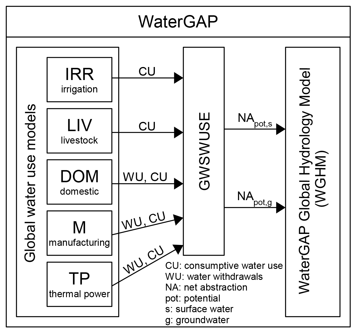
Figure 1The WaterGAP 2.2d framework with its water use models and the linking module GWSWUSE that provides potential net water abstraction from groundwater and surface water as input to the WaterGAP Global Hydrology Model (WGHM). Figure adapted from Müller Schmied et al. (2014).
2.1 Spatial coverage and climate forcings
The WaterGAP 2 framework operates on the so-called CRU land–sea mask (Mitchell and Jones, 2005), which covers the global continental area (including small islands and Greenland but excluding Antarctica) with 67 420 grid cells in total, each 0.5∘ × 0.5∘ in size, which represents approx. 55 km × 55 km at the Equator. WaterGAP uses the continental area of the grid cell, which is defined as the cell area (calculated with equal area cylindrical projection) minus the ocean area with the borders according to the ESRI worldmask shapefile (ArcGIS, 2018). The continental area comprises land area and surface water body area (lakes, reservoirs and wetlands only; river area is not considered). Since WaterGAP 2.2a, surface water body areas, and consequently land area, are dynamic and are updated in each time step.
Both GIM and WGHM use meteorological input data that consist of air temperature, precipitation, downward shortwave radiation and downward longwave radiation, all with daily temporal resolution. Various global meteorological datasets (hereafter referred to as climate forcings) were developed by the meteorological community at the 0.5∘ × 0.5∘ spatial resolution, such as WFD (Weedon et al., 2011), WFDEI (Weedon et al., 2014), GSWP3 (Kim, 2014), the Princeton meteorological forcing (Sheffield et al., 2006), and recently ERA5 (Hersbach et al., 2020) and WFDE5 (Cucchi et al., 2020). Alternative climate forcings may lead to significantly different WaterGAP outputs (Müller Schmied et al., 2016a).
2.2 Modifications of WaterGAP since version 2.2
The general framework of WaterGAP 2.2d does not differ from model version 2.2 described in Müller Schmied et al. (2014). Improvements of water use modeling since WaterGAP 2.2 include, among others, deficit irrigation in regions with groundwater depletion (Sect. 3.3) as well as integration of the Historical Irrigation Dataset (HID), which provides the historical cell-specific development of the area equipped for irrigation (Siebert et al., 2015). Major improvements in WGHM include (1) a consistent river-storage-based method to compute river flow velocity; (2) simulation of land area dynamics in response to varying areas of lakes, reservoirs and wetlands; (3) groundwater recharge from these surface water bodies in (semi)arid grid cells; (4) if daily precipitation is below a threshold value, the potential groundwater recharge remains in the soil and does not (as in WaterGAP 2.2) become surface runoff; (5) return flows to groundwater from surface water use are corrected (by adjusting NAg) by the amount of NApot,s that cannot be satisfied; and (6) the integration of reservoirs by taking into account their commissioning year (and not assuming anymore that they have existed during the whole study period). Other changes concern model calibration or consist of the inclusion of new datasets and software improvements. A complete list of modifications of WaterGAP 2.2d compared to WaterGAP 2.2 is provided in Appendix A.
3.1 Global Irrigation Model
Irrigation accounts for 60 %–70 % of global withdrawal water uses and 80 %–90 % of global consumptive water uses, and for even larger shares in almost all regions with severe water stress and groundwater depletion (Döll et al., 2012, 2014). Therefore, a reliable simulation of irrigation water use is decisive for the quality of WaterGAP simulations of streamflow and water storage in groundwater and surface water bodies as well as for the reliability of computed water stress indicators. Based on information on irrigated area and climate for each grid cell, GIM computes first cell-specific cropping patterns and growing periods and then irrigation consumptive water use (ICU), distinguishing only rice and non-rice crops (Döll and Siebert, 2002). ICU can be regarded as the net irrigation requirement that would lead to optimal crop growth.
3.1.1 Computation of cropping patterns and growing periods of rice and non-rice crops
The cropping pattern for each cell with irrigated cropland describes whether only rice, non-rice crops or both are irrigated during either one or two growing seasons. The growing period for both crop types is assumed to be 150 d. A total of 17 cropping patterns are possible including simple variants (e.g., one cropping season with non-rice on the total irrigated area) and complex variants (non-rice after rice on one part of the total irrigated area and non-rice after non-rice on the other). The following data are used to model the cropping pattern: total irrigated area, long-term average temperature and soil suitability for paddy rice in each cell, harvested area of irrigated rice in each country, and cropping intensity in each of 19 world regions. In a second step, the optimal start date of each growing season is computed for each crop. To this end, each 150 d period within a year is ranked based on criteria of long-term average temperature, precipitation and potential evapotranspiration provided in Döll and Siebert (2002). The most highly ranked 150 d period(s) is (are) defined as growing season(s).
3.1.2 Computation of consumptive water use due to irrigation
GIM implements the Food and Agriculture Organization of the United Nations (FAO) CROPWAT approach of Smith (1992) to compute crop-specific ICU per unit irrigated area (mm d−1) during the growing season as the difference between crop-specific optimal evapotranspiration and effective precipitation Pirri,eff if the latter is smaller than the former, with
where is the product of potential evapotranspiration Epot and the dimensionless crop coefficient kc which depends on the crop and the crop development stage (Döll and Siebert, 2002). As a standard, Epot is calculated according to Eq. (7). Pirri,eff is the fraction of the total precipitation P (including rainfall and snowmelt) that is available to plants and is computed as a simple empirical function of precipitation. Equation (1) is implemented with a daily time step, but to take into account the storage capacity of the soil and to remain consistent with the CROPWAT approach, daily precipitation values are averaged over 10 d, except for rice-growing areas in Asia, where the averaging period is only 3 d to represent the limited soil water storage capacity in the case of paddy rice (Döll and Siebert, 2002).
3.1.3 Irrigated area
In the standard version of WaterGAP 2.2d, irrigated area per grid cell used in GIM is based on the HID (Siebert et al., 2015), which provides area equipped for irrigation (AEI) in 5 arcmin grid cells for 14 time slices between 1900 and 2005. HID data are aggregated to 0.5∘ × 0.5∘ and temporally interpolated to obtain an annual time series of AEI. Cropping patterns and growing periods are generated for every year, with an individual combination of year-specific AEI and harvested area of rice and the respective 30-year climate averages, which are then used to calculate ICU for every day of the same year (Sect. 3.1.1). Harvested area of rice per country from the MIRCA2000 dataset, representative for the year 2000 (Portmann et al., 2010), is scaled according to annual AEI country totals, ensuring consistency to AEI.
To take into account that not the whole AEI is actually used for irrigation in any year, country-specific values of the ratio of area actually irrigated (AAI) to AEI are used to estimate AAI in each grid cell. AAI is then applied for calculating the consumptive irrigation water use in volume per time. AAI AEI ratios were derived from the Global Map of Irrigation Area (GMIA) for 2005 (Siebert et al., 2013). To set AAI from 2006 to 2016, we found country-specific AAI for 2006–2008 from the AQUASTAT database of the FAO, other international organizations, and national statistical services (e.g., EUROSTAT and USDA) for 61 countries. For these countries, the AAI values for 2009–2016 were set to the 2008 values, while for the rest of the countries, AAI was set to the 2005 values for the whole period 2006–2016.
Alternatively, as in previous WaterGAP versions, GIM in WaterGAP 2.2d can be executed based on a temporally constant dataset of AEI per grid cell, e.g., the GMIA for 2005 (Siebert et al., 2013). Cropping patterns and growing periods are then computed for AEI and harvested area of rice in a reference year and the pertaining 30-year average climate. For more details and application examples, we refer to Portmann (2017) and Döll and Siebert (2002).
3.2 Non-irrigation water uses
Although irrigation water use is the dominant water use sector globally, non-irrigation water uses, particularly in terms of withdrawal water uses, play a major role in Europe and America (FAO, 2016). Competition between agricultural and non-agricultural water uses are not uncommon (Flörke et al., 2018), and the estimation of water demands becomes even more crucial when water resources are scarce. Statistical information on withdrawal water uses and consumptive water uses for domestic, industrial and livestock purposes are difficult to obtain on a country basis since no comprehensive global database does exist. However, the FAO collects relevant water-related data from national statistics and reports to provide a comprehensive view on the state of sectoral water uses. Unfortunately, the database lacks data in space and time, and hence modeling is of importance to fill these gaps (Flörke et al., 2013).
3.2.1 Livestock
Withdrawal water uses for livestock are computed annually by multiplying the number of animals per grid cell by the livestock-specific water use intensity (Alcamo et al., 2003). The number of livestock are taken from FAOSTAT (2014). It is assumed that the withdrawal water uses for livestock are equal to their consumptive water use.
3.2.2 Domestic
Domestic water use comprises withdrawal water uses and consumptive water uses of households and small businesses and is estimated on a national level. The main concept is to first compute the domestic water use intensity (m3 per capita per year) and then to multiply this by the population of water users in a country. The domestic water use intensity is expressed by a sigmoid curve which indicates how water use intensity (per capita water use) changes with income (gross domestic product per capita) and is derived from historical data on a national or regional level (Flörke et al., 2013). Besides changes driven by income and population, technological changes are considered to reflect improvement in water-use efficiency. Continuous improvements in technology make appliances more water efficient and, hence, contribute to reductions in water use. Detailed data on domestic consumptive water uses do not exist from statistics, but a simple balancing equation has been used in WaterGAP since the year 2000 to simulate consumptive water uses as the difference between withdrawal water use and wastewater volume (i.e., return flow) as the latter information is available from statistics. The calculation of consumptive water use before the year 2000 is based on the application of consumptive water use coefficients (Shiklomanov, 2000) that accounts for the proportion of the withdrawal water use that is consumed. In order to allow for a spatially explicit analysis, country values of domestic water uses are allocated to grid cells (0.5∘ × 0.5∘) within the country based on the geo-referenced historical population density maps from HYDE version 3.1 (Goldewijk et al., 2010). Additionally, population numbers beyond 2005 as well as information on the ratio of rural to urban population of each grid cell come from UNEP (2015).
3.2.3 Manufacturing
The manufacturing sector is rather diverse in terms of water use and varies between countries and subsectors, for example highly water-intensive production processes in the chemical industry compared to the processes in the glass industry that use less water. In WaterGAP, the manufacturing water use model simulates the annual withdrawal water use and consumptive water use of water that is used for production and cooling processes, whereas the water used for power generation is modeled separately. A manufacturing structural water intensity that describes the ratio of water abstracted over the manufacturing gross value added (GVA) is derived per country for the base year 2005 (in m3 USD (constant for the year 2000)−1) based on national statistics (Flörke et al., 2013). GVA is found to be positively correlated with the sector's withdrawal water uses (Dziegielewski et al., 2002) and is used as the driving force to reflect the time variant system. In addition, technological improvements are considered through a technological change factor.
The consumptive water use for this sector is obtained by using the same approach as described for the domestic sector, i.e., the calculation of the difference between the withdrawal water use and the return flows (starting in the year 2000) and the application of a consumption factor before the year 2000. Contrary to the domestic sector, return flows from the manufacturing sector are further subdivided into cooling water and wastewater. For countries where no data are available, the fraction of consumptive water use is derived from neighboring or economically comparable countries. Less information is available on the location of manufacturing industries; therefore country-level manufacturing water use is downscaled to grid cells proportional to its urban population (Flörke et al., 2013).
3.2.4 Thermal power
Water is abstracted and consumed for the production of thermal electricity, particularly for cooling purposes where water is used to condense steam from the turbine exhaust. The volume of cooling withdrawal water use and consumptive water use is modeled on a grid-cell level based on input data on the location, type and size of power stations from the World Electric Power Plant Database (UDI, 2004). Here, the annual cooling water requirements in each grid cell are calculated by multiplying the annual thermal electricity production with the respective water-use intensity of each power station (Flörke et al., 2013). A key driver is the annual thermal electricity production (MWh yr−1) on a country basis, which is downscaled to the level of thermal power plants according to their capacities. Time series on thermal electricity production per country until 2010 are available online from the Energy Information Administration (EIA, 2012). Cooling water intensities in terms of withdrawal water use and consumptive water use vary between plant types and cooling systems. Therefore, the model distinguishes between four plant types (biomass and waste, nuclear, natural gas and oil, coal, and petroleum) and three cooling systems (tower cooling, once-through cooling, ponds) (Flörke et al., 2012). The approach is complemented by considering technological change leading to reduced intensities.
In general, water abstractions of once-through flow systems are considerably higher compared to the withdrawal intensities of pond cooling or tower cooling systems. In contrast, consumptive water use of tower cooling systems is much higher than water consumed by once-through cooling systems. In ordering plant-type-specific water intensities, i.e., water abstraction per unit electricity production, it becomes obvious that intensities are highest for nuclear power plants, followed by fossil, biomass, and waste-fuelled steam plants, while natural gas and oil combined-cycle plants have the lowest intensities, respectively. The model has been validated for the year 2005 by comparing modeled values with published thermoelectric withdrawal water uses (Flörke et al., 2013).
3.3 GWSWUSE
The linking model GWSWUSE computes the fractions of all five sectoral water abstractions, or withdrawal water use, WU and consumptive water use CU in each grid cell that stem from either groundwater or surface water bodies (lakes, reservoirs and river). Time series for WU and CU from the sectoral water use models are an input to GWSWUSE except for WU for irrigation. The latter is computed within GWSWUSE as water use efficiencies CU/WU for irrigation are assumed to vary between surface water and groundwater. Country-specific efficiency values are used for surface water irrigation, while in the case of groundwater irrigation, water use efficiency is set to a relatively high value of 0.7 worldwide (Döll et al., 2014). In GWSWUSE, CU due to irrigation is decreased to 70 % of optimal CU in groundwater depletion areas; these areas were defined as grid cells with a groundwater depletion rate for 1980–2009 of more than 5 mm yr−1 and a ratio of WU for irrigation over WU for all sectors of more than 5 % as computed for optimal irrigation in Döll et al. (2014).
Sectoral groundwater fractions were derived individually for each grid cell in the case of irrigation (Siebert et al., 2010) and for each country in the case of the other four water use sectors (Döll et al., 2012). They are assumed to be temporally constant. Water for livestock and the cooling of thermal power plants is assumed to be extracted exclusively from surface water bodies.
Finally, GWSWUSE computes monthly time series of net abstraction from surface water NApot,s and from groundwater NApot,g which are used as input to WGHM. Net abstraction is the difference between total water abstraction from one of the two sources and the return flow to the respective source according to Eqs. (1), (3) and (4) in Döll et al. (2012). In all sectors except irrigation, return flows are only directed to surface water bodies. The fraction of return flow to groundwater in the case of irrigation water use is estimated as a function of degree of artificial drainage in the grid cell (Sect. 2.1.3 in Döll et al., 2014). Positive net abstraction values refer to the situation where storage is reduced due to human water use, and negative values indicate an increase in storage. In the case of groundwater, the latter only occurs if there is irrigation with surface water in the grid cell. The approach of direct net abstractions implicitly assumes instantaneous return flows. The sum of NApot,g and NApot,s is equivalent to (potential) consumptive water use. NApot,s and NApot,g as computed by GWSWUSE are potential net abstractions that may be adjusted depending on the availability of surface water (Sect. 4.8).
The WGHM simulates daily water flows and water storage in 10 compartments (Fig. 2). The vertical water balance (dashed box in Fig. 2) encompasses the canopy (Sect. 4.2), snow (Sect. 4.3) and soil (Sect. 4.4) components. Water storage in glaciers is not simulated by WaterGAP 2.2d. The lateral water balance includes groundwater (Sect. 4.5), lakes, man-made reservoirs, wetlands (Sect. 4.6) and rivers (Sect. 4.7). Different to the vertical water balances, where the water balance is calculated based on water height units (mm), the lateral water balance is calculated in volumetric units (m3). Water height units are converted to volumetric units by considering the land area (for flows) or continental area (for storages) of the grid cell, respectively. Local surface water bodies are defined to be recharged only by runoff generated in the cell itself, while global ones additionally receive streamflow from upstream cells (Fig. 2). Upstream–downstream relations among the grid cells are defined by the drainage direction map DDM30 (Döll and Lehner, 2002). Each cell can drain only into one of the eight neighboring cells as streamflow. There is no groundwater flow between grid cells.
The amount of water reaching the soil is regulated by the canopy and snow water balance. Total runoff from the land fraction of the cell Rl is calculated from the soil water balance. Rl is then partitioned into fast surface and subsurface runoff Rs and diffuse groundwater recharge Rg. Lateral routing of water through the storage compartments is based on the so-called fractional routing scheme (Döll et al., 2014) and differs between (semi)arid and humid grid cells (red and green arrows in Fig. 2). The definition of (semi)arid and humid cells is given in Appendix B. To avoid that all runoff generated in the grid cell is added to local lake or wetland storage, only the fraction fswb times Rs flows into surface water bodies, and the remainder discharges into the river. The factor fswb is calculated as the relative area of wetlands and local lakes in a grid cell multiplied by 20 (representing the drainage area of surface water bodies), with its maximum value limited to the cell fraction of continental area. In humid cells, groundwater discharge Qg is partitioned using fswb into discharge to surface water bodies and discharge to the river segment. In (semi)arid cells, surface water bodies (excluding rivers) are assumed to recharge the groundwater to mimic point recharge. To avoid a short circuit between groundwater and surface water bodies, the whole amount of Qg flows into the river. Loosing conditions, where river water recharges the groundwater, are not modeled in WGHM.
In WaterGAP, human water use is assumed to affect only the water storages in the lateral water balance. Increases in soil water storage in irrigated areas are not taken into account as the WaterGAP approach of direct net abstractions implicitly assumes instantaneous return flows. To consider anthropogenic consumptive water use in the output variable of actual evapotranspiration Ea (Table 2), we sum up all evapo(transpi)ration components and actual consumptive water use WCa (see note 5 in Table 2). NAs is abstracted from the different surface water bodies except wetlands with the priorities shown as numbers in Fig. 2.
Outflow from the final water storage compartment in each cell, the river compartment, is streamflow (Qr,out), which becomes inflow into the next downstream cell.
The ordinary differential equations describing the water balances of the 10 storage compartments simulated in WGHM are solved sequentially for each daily time step in the following order: canopy, snow, soil, groundwater, local lakes, local wetlands, global lakes, global reservoirs/regulated lakes, river (Fig. 2). An explicit Eulerian method is used to numerically solve all differential equations except those for global lakes and rivers, where an analytical solution is applied to compute storage change during one daily time step, which allows daily time steps instead of smaller time steps that would have been required in the case of an explicit Eulerian method. As the water balances of global lakes, global reservoirs/regulated lakes and river of a grid cell are not independent from those of the upstream grid cells, the sequence of grid cell computations starts at the most upstream grid cells and continues downstream according to the drainage direction map DDM30 (Döll and Lehner, 2002).
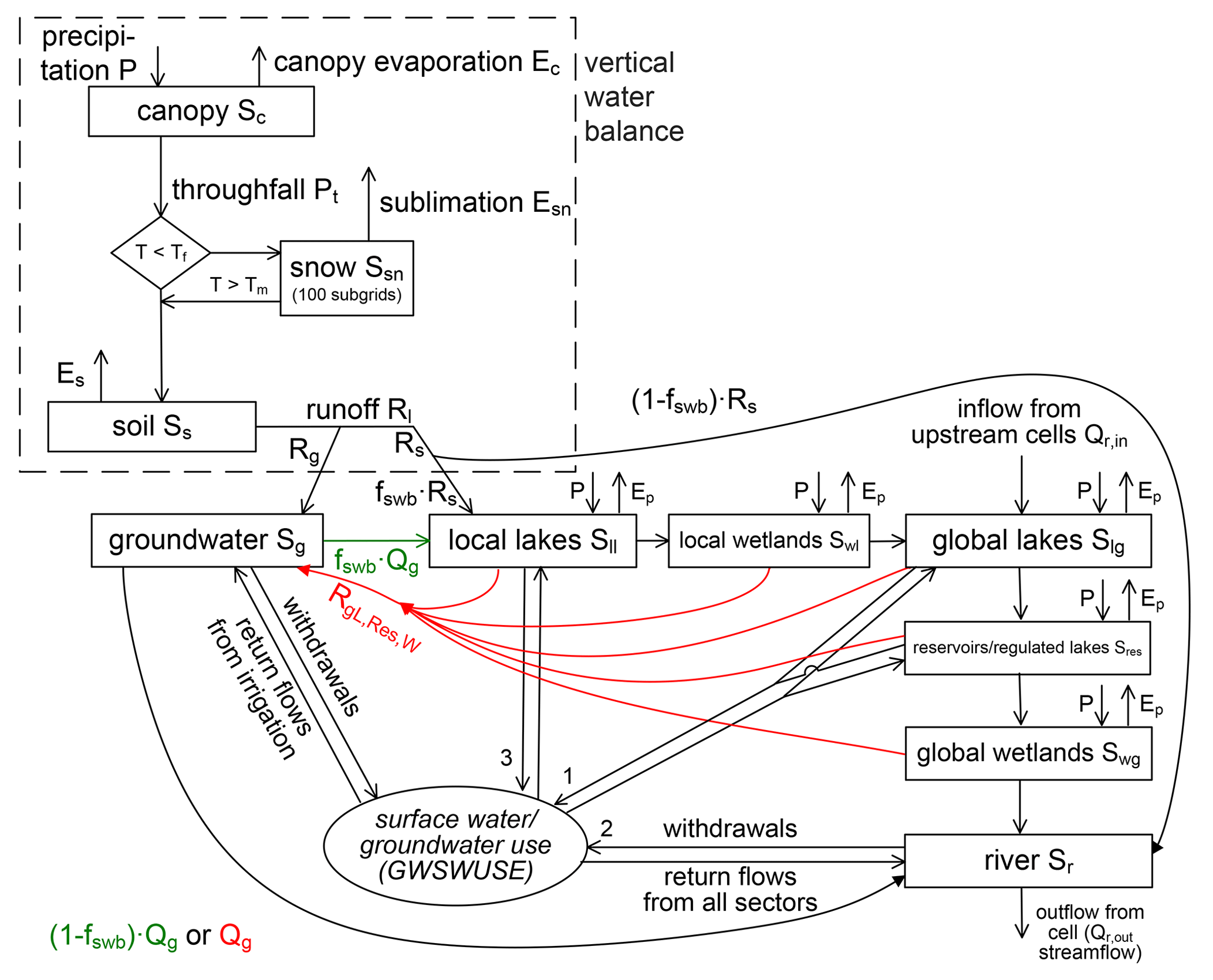
Figure 2Schematic of WGHM in WaterGAP 2.2d. Boxes represent water storage compartments, and arrows represent water flows. Green (red) color indicates processes that occur only in grid cells with humid ((semi)arid) climate. For details the reader is referred to Sect. 4.2 to 4.8, in which the water balance equations of all 10 water storage compartments are presented.
4.1 General model variants of human water use and reservoirs
The standard model setup of WGHM in WaterGAP 2.2d simulates the effects of both human water use and man-made reservoirs (including their commissioning years) on flows and storages and is referred to as “ant” simulation (anthropogenic). These stressors can be turned off in alternative model setups to simulate a world without these two types of human activities and to quantify the direct impact of human water use and reservoirs.
-
“Nat” simulations compute naturalized flows and storages that would occur if there where neither human water use nor global man-made reservoirs/regulated lakes.
-
“Use only” simulations include human water use but exclude global man-made reservoirs/regulated lakes.
-
“Reservoirs only” simulations exclude human water use but include global man-made reservoirs/regulated lakes.
The following sections generally refer to ant simulations.
4.2 Canopy
Canopy refers to the leaves and branches of terrestrial vegetation that intercept precipitation. Modeling of the canopy processes does not differentiate between rain and snow.
4.2.1 Water balance
The canopy storage Sc (mm) is calculated as
where P is precipitation (mm d−1); Pt is throughfall, the fraction of P that reaches the soil (mm d−1); and Ec is evaporation from the canopy (mm d−1).
4.2.2 Inflows
Daily precipitation P is read in from the selected climate forcing (see Sect. 7.1).
4.2.3 Outflows
Throughfall Pt is calculated as
where Sc,max is maximum canopy storage calculated as
where mc is 0.3 mm (Deardorff, 1978), and L (−) is the one-side leaf area index. L is a function of daily temperature and P and limited to minimum or maximum values. Maximum L values per land cover class (Table C1) are based on Schulze et al. (1994) and Scurlock et al. (2001), whereas minimum L values are calculated as
where fd,lc is the fraction of deciduous plants and ce,lc is the reduction factor for evergreen plants per land cover type (Table C1).
The growing season starts when daily temperature is above 8 ∘C for a land-cover-specific number of days (Table C1) and cumulative precipitation from the day where growing season starts reaches at least 40 mm. In the beginning of the growing season, L increases linearly for 30 d until it reaches Lmax. For (semi)arid cells, at least 0.5 mm of daily P is required to keep the growing season on-going. When growing season conditions are not fulfilled anymore, a senescence phase is initiated and L linearly decreases to Lmin within the next 30 d (Kaspar, 2004). It is noteworthy that in WaterGAP L only affects the calculation of the canopy water balance. L is not taken into account in computing consumptive water use for irrigated crops (Sect. 3.1) and evapotranspiration from land (Sect. 4.4).
Following Deardorff (1978), Ec is calculated as
where Epot is the potential evapotranspiration (mm d−1) calculated with the Priestley–Taylor equation according to Shuttleworth (1993) as
where, following Shuttleworth (1993), α is set to 1.26 in humid and to 1.74 in (semi)arid cells (Appendix B). R is net radiation (mm d−1) that depends on land cover (Table C2) (for details on the calculation of net radiation, the reader is referred to Müller Schmied et al., 2016b), and sa is the slope of the saturation vapor pressure–temperature relationship () defined as
where T (∘C) is the daily air temperature and g is the psychrometric constant (). The latter is defined as
where pa is atmospheric pressure of the standard atmosphere (101.3 kPa), and lh is latent heat (MJ kg−1). Latent heat is calculated as
4.3 Snow
To simulate snow dynamics, each 0.5∘ × 0.5∘ grid cell is spatially disaggregated into 100 non-localized subcells that are assigned different land surface elevations according to GTOPO30 (U.S. Geological Survey, 1996). Daily temperature at each subcell is calculated from daily temperature at the 0.5∘ × 0.5∘ cell by applying an adiabatic lapse rate of 0.6 ∘C per 100 m (Schulze and Döll, 2004). The daily snow water balance is computed for each of the subcells such that within a 0.5∘ × 0.5∘ cell there may be subcells with and without snow cover or snowfall. For model output, subcell values are aggregated to 0.5∘ × 0.5∘ cell values.
4.3.1 Water balance
Snow storage accumulates below snow freeze temperature and decreases by snow melt and sublimation. Snow storage Ssn (mm) is calculated as
where Psn is the part of Pt that falls as snow (mm d−1), M is snowmelt (mm d−1) and Esn is sublimation (mm d−1).
4.3.2 Inflows
Snowfall Psn (mm d−1) is calculated as
where T is daily air temperature (∘C), and Tf is snow freeze temperature, set to 0 ∘C. In order to prevent excessive snow accumulation, when snow storage Ssn reaches 1000 mm in a subcell, the temperature in this subcell is increased to the temperature in the highest subcell with a temperature above Tf (Schulze and Döll, 2004).
4.3.3 Outflows
Snow melt M is calculated with a land-cover-specific degree-day factor DF () (Table C2) when the temperature T in a subgrid surpasses melting temperature Tm (∘C), set to 0 ∘C, as
Sublimation Esn is calculated as the fraction of Epot that remains available after Ec. For calculating Epot according to Eq. (7), land-cover-specific albedo values are used if Ssn surpasses 3 mm in the 0.5∘ × 0.5∘ cell (Table C2).
4.4 Soil
WaterGAP represents soil as a one-layer soil water storage compartment characterized by a land-cover- and soil-specific maximum storage capacity as well as soil texture. The simulated water storage represents soil moisture in the effective root zone.
4.4.1 Water balance
The change of soil water storage Ss (mm) over time (d) is calculated as
where Peff is effective precipitation (mm d−1), Rl is runoff from land (mm d−1) and Es is actual evapotranspiration from the soil (mm d−1). Once the water balance is computed, Rl is partitioned into (1) fast surface and subsurface runoff Rs, representing direct surface runoff and interflow, and (2) groundwater recharge Rg (Fig. 2) according to a heuristic scheme (Döll and Fiedler, 2008).
4.4.2 Inflows
Peff is computed as
where Pt is throughfall (mm d−1; see Eq. 3), Psn is snowfall (mm d−1; see Eq. 12) and M is snowmelt (mm d−1; see Eq. 13).
4.4.3 Outflows
Es is calculated as
where Epot is potential evapotranspiration (mm d−1), Ec is canopy evaporation (mm d−1; Eq. 6) and Ss,max is the maximum soil water content (mm) derived as a product of total available water capacity in the upper meter of the soil (Batjes, 2012) and land-cover-specific rooting depth (Table C2) (Müller Schmied, 2017). Epot,max is set to 15 mm d−1 globally. Following Bergström (1995), runoff from land Rl is calculated as
where γ is the runoff coefficient (–). This parameter, which varies between 0.1 and 5.0, is used for calibration (Sect. 4.9). Together with soil saturation, it determines the fraction of Peff that becomes Rl (Fig. 3). If the sum of Peff and Ss of the previous day exceed Ss,max, the exceeding fraction of Peff is added to Rl. In urban areas (defined from MODIS data, Sect. C), 50 % of Peff is directly turned into Rl.
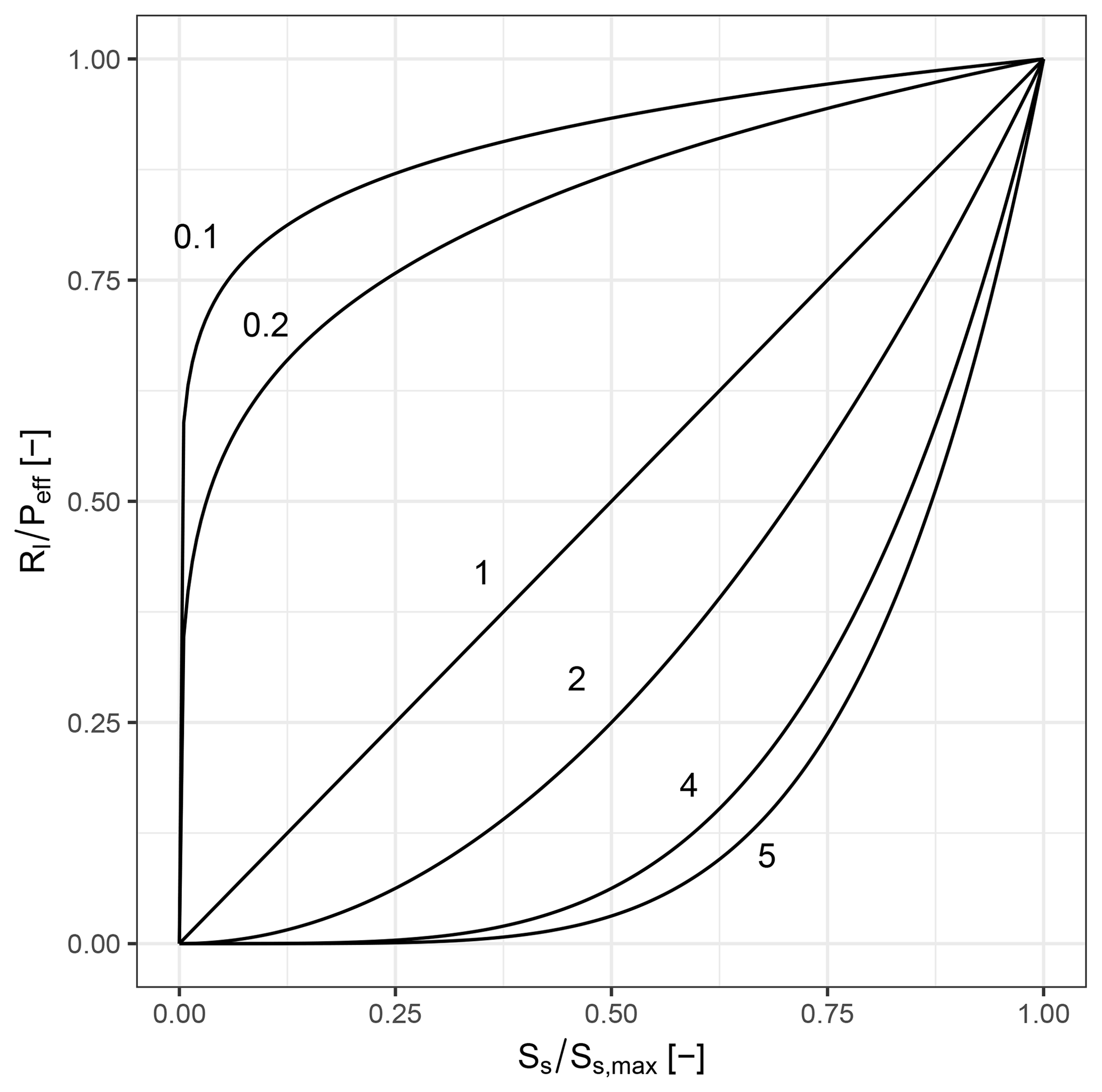
Figure 3Relation between runoff from land Rl as a fraction of effective precipitation Peff and soil saturation for different values of the runoff coefficient γ in WaterGAP.
Rl is partitioned into fast surface and subsurface runoff Rs and diffuse groundwater recharge Rg calculated as
where is soil-texture-specific maximum groundwater recharge with values of 7, 4.5 and 2.5 mm d−1 for sandy, loamy and clayey soils, respectively, and fg is the groundwater recharge factor ranging between 0 and 1. fg is determined based on relief, soil texture, aquifer type, and the existence of permafrost or glaciers (Döll and Fiedler, 2008). If a grid cell is defined as (semi)arid and has coarse (sandy) soil, groundwater recharge will only occur if precipitation exceeds a critical value of 12.5 mm d−1, otherwise the water remains in the soil. The fraction of Rl that does not recharge the groundwater becomes Rs, which recharges surface water bodies and the river compartment.
4.5 Groundwater
As there is no knowledge about the depth below the land surface where groundwater no longer occurs due to the lack of pore space, groundwater storage can only be computed in relative terms but is assumed to be unlimited. The groundwater storage Sg is always positive unless net abstractions from groundwater NAg are high and groundwater depletion occurs. Groundwater discharge is assumed to be proportional to (positive) Sg and to stop in the case of negative Sg.
4.5.1 Water balance
The temporal development of groundwater storage Sg (m3) is calculated as
where Rg is diffuse groundwater recharge from soil (m3 d−1, Eq. 19), is point groundwater recharge from surface water bodies (lakes, reservoirs and wetlands) in (semi)arid areas (m3 d−1, Eq. 26), Qg is groundwater discharge (m3 d−1) and NAg is net abstraction from groundwater (m3 d−1).
4.5.2 Inflows
Rg is the main inflow in most grid cells, except in (semi)arid grid cells with significant surface water bodies where may be dominant. varies temporally with the area of the surface water body, which depends on the respective water storage (Sect. 4.6). In many cells with significant irrigation with surface water, NAg is negative, and irrigation causes a net inflow into the groundwater due to high return flows (Sect. 3.3).
4.5.3 Outflows
Qg quantifies the discharge from groundwater storage to surface water storage, with
where kg=0.01 d−1 is the globally constant groundwater discharge coefficient (Döll et al., 2014). The second outflow component NAg is described in Sect. 3.3.
4.6 Lakes, man-made reservoirs and wetlands
Where lakes, man-made reservoirs and wetlands (LResWs) of significant size exist, their water balances strongly affect the overall water balance of the grid cell due to their high evaporation and water retention capacity (Döll et al., 2003). WGHM uses the Global Lakes and Wetland Database (GLWD) (Lehner and Döll, 2004) and a preliminary but updated version of the Global Reservoir and Dam (GRanD) database (Döll et al., 2009; Lehner et al., 2011) to define location, area and other attributes of LResWs. It is assumed that surface areas given in the databases represent the maximum extent. Appendix D describes how the information from these databases is integrated into WGHM. Two categories of LResWs are defined for WGHM, so-called “local” water bodies that receive inflow only from the runoff generated within the grid cell and so-called “global” water bodies that additionally receive the streamflow from the upstream grid cells (Fig. 2). Six different LResW types are distinguished in WaterGAP.
-
Local wetlands (wl) and global wetlands (wg). These cover a maximum area of 3.743 million km2 and 3.752 million km2, respectively, an area that is at its maximum at least 3 times larger than the combined maximum area of lakes and reservoirs (Appendix D). However, 0.3 million km2 of floodplains along large rivers is included as global wetlands, and their dynamics are not simulated suitably by WGHM. They are assumed to receive the total streamflow as inflow while in reality only the part of the streamflow that does not fit in the river channel flows into the floodplain (Döll et al., 2020). All local (global) wetlands within a 0.5∘ × 0.5∘ grid cell are simulated as one local (global) wetland that covers a specified fraction of the cell.
-
Local lakes (ll). These include about 250 000 small lakes and more than 5000 man-made reservoirs and are defined to have a surface area of less than 100 km2 or a maximum storage capacity of less than 0.5 km3. Like wetlands, all local lakes in a grid cell are aggregated and simulated as one storage compartment taking up a fraction of the grid cell area. Small reservoirs are simulated like lakes as (1) the required lumping of all local reservoirs within a grid cell into one local reservoir per cell necessarily leads to a “blurring” of the specific reservoir characteristics, and (2) small reservoirs are likely not on the main river simulated in the grid cell but on a tributary. Therefore, a reservoir algorithm is not expected to simulate water storage and flows better than the lake algorithm.
-
1355 global lakes (lg). These consist of lakes with an area of more than 100 km2, are simulated in WaterGAP. Since a global lake may spread over more than one grid cell, the water balance of the whole lake is computed at the outflow cell (Döll et al., 2009) (for consequences, see Sect. 5.2). Only the maximum area of natural lakes is known, not the maximum water storage capacity.
-
Global man-made reservoirs (res) and global regulated lakes. Global man-made reservoirs have a maximum storage capacity of at least 0.5 km3, and global regulated lakes (lakes where outflow is controlled by a dam or weir) have a maximum storage capacity of at least 0.5 km3 or an area of more than 100 km2. Both are simulated by the same water balance equation. There can be only one global reservoir/regulated lake compartment per grid cell. Outflow from reservoirs/regulated lakes is simulated by a modified version of the Hanasaki et al. (2006) algorithm, distinguishing reservoirs/regulated lakes with the main purpose of irrigation from others (Döll et al., 2009). Like in the case of global lakes, water balance of global reservoirs/regulated lakes is computed at the outflow cell (for consequences; see Sect. 5.2). Different from lakes, information on maximum water storage capacity is available from the GRanD database, in addition to the main use and the commissioning year. In WGHM, reservoirs start filling at the beginning of the commissioning year, and regulated lakes then turn from global lakes into global regulated lakes (Appendix D). A total of 1082 global reservoirs and 85 regulated lakes are taken into account, but as those that have the same outflow cell are aggregated to one water storage compartment by adding maximum storages and areas, only 1109 global reservoirs/regulated lakes compartments are simulated in WGHM (Appendix D). Under naturalized conditions (Sect. 4.1), there are no global man-made reservoirs, and regulated lakes are simulated as global lakes; however, local reservoirs remain in the model.
In each grid cell, there can be a maximum of one local wetland storage compartment, one global wetland compartment, one local lake compartment, one global lake compartment and one global reservoir/regulated lake compartment. The lateral water flow within the cell follows the sequence shown in Fig. 2. For example, if there is a local lake compartment in a grid cell, it is this compartment that receives, under a humid climate, a fraction of the outflow from the groundwater compartment and of the fast surface and subsurface outflow, and the outflow from the local lake becomes inflow to the local wetland if it exists (Fig. 2). If there is no local wetland but a global lake, the outflow from the local lake becomes part of the inflow of the global lake. In the case of having a global lake and a global reservoir/regulated lake in one cell, water is routed first through the global lake.
4.6.1 Water balance
The water balance for the five types of LResW compartments is calculated as
where is volume of water stored in the water body (m3), Qin is inflow into the water body from upstream (m3 d−1), A is global (or local) water body surface area (m2) in the grid cell at time t, P is precipitation (m3 d−1), Epot is potential evapotranspiration (m3 d−1, Eq. 7), is groundwater recharge from the water body (only in arid/semiarid regions) (m3 d−1, Eq. 26), NAl,res is the net abstraction from the lakes and reservoirs (m3 d−1) (Fig. 2 and Sect. 4.8), and Qout is outflow from the water body to other surface water bodies including river storage (m3 d−1) (Fig. 2).
The temporally varying surface area A of the water body is computed in each daily time step using the following equation:
where r is reduction factor (–), and Amax is maximum extent of the water body (m2) from GRanD or GLWD databases. In the case of local and global lakes
where Sl is the volume of the water (m3) stored in the lake at time t (d), Sl,max is the maximum storage of the lake (m3), Sl,max is computed based on Amax and a maximum storage depth of 5 m, and p is the reduction exponent (–), set to 3.32. According to the above equation, the area is reduced by 1 % if Sl=50 % of Sl,max, by 10 % if Sl=0 and by 100 % if (Hunger and Döll, 2008). In the case of global reservoirs/regulated lakes and local and global wetlands
where Sres,w is the volume of the water (m3) stored in the reservoir/regulated lake or wetland, and p is 2.814 and 3.32 for reservoirs/regulated lakes and wetlands, respectively. In the case of wetlands, (m3) is computed based on Amax and a maximum storage depth of 2 m. Wetland area is reduced by 10 % if Sw=50 % of and by 70 % if Sw is only 10 % of . In the case of reservoirs/regulated lakes, storage capacity is taken from the database. Reservoir area is reduced by 15 % if Sres is 50 % of and by 75 % if Sres is only 10 % of . For regulated lakes without available maximum storage capacity, is computed as in the case of global lakes.
While storage in reservoirs/regulated lakes and wetlands cannot drop below zero due to high outflows, high evaporation or NAs, storage in lakes can become negative. This represents the situation where there is no more outflow from the lake to a downstream water body (Qout=0). There, like groundwater storage, storage of local and global lakes is a relative and not an absolute water storage. Reservoir/regulated lake storage is not allowed to fall below 10 % of storage capacity.
With changing A of the surface water compartments local wetland, global wetlands and local lakes, the land area fraction is adjusted accordingly. However, in the case of global lakes and reservoirs/regulated lakes, which may cover more than one 0.5∘ × 0.5∘ cell, such an adjustment is not made as it is not known in which grid cells the area reduction occurs. Therefore, land area fraction is not adjusted with changing r and precipitation is assumed to fall on a surface water body with an area of Amax instead of A.
4.6.2 Inflows
Calculation of Qin differs between local and global water bodies. In the case of local lakes and local wetlands, they are recharged only by local runoff generated within the same grid cell. A fraction fswb of the fast surface and subsurface runoff generated within the grid cell Rs (m3 d−1) and, only in the case of humid grid cells, a fraction fswb of the base flow from groundwater Qg (m3 d−1) become inflow to local water bodies (Fig. 2, Sect. 4.4.3, 4.5.2). In the case where one grid cell contains both local lake and wetland, then the outflow of the local lake will be the inflow to the local wetland according to Fig. 2. Global lakes, global wetlands, and global reservoirs/regulated lakes receive, in addition to local runoff, inflow from streamflow of the upstream grid cells as river inflow (Fig. 2). In many cells with significant groundwater abstraction, NAs is negative, and return flow leads to a net inflow into surface water bodies (Sect. 3.3).
4.6.3 Outflows
LResWs lose water by evaporation Epot, which is assumed to be equal to the potential evapotranspiration computed using the Priestley–Taylor equation with an albedo of 0.08 according to Eq. (7). In semiarid and arid grid cells (Appendix B), LResWs are assumed to recharge the groundwater with a focused groundwater recharge, with
where is the groundwater recharge constant below LResWs (=0.01 m d−1). This process is applied only in the arid and semiarid grid cells, as in humid areas groundwater mostly recharges the surface water bodies as explained in Sect. 4.6.2 (Döll et al., 2014).
It is assumed that water can be abstracted from lakes and reservoirs but not from wetlands. An amount of NAl,res (m3 d−1) is the net abstractions from lakes and reservoirs, which depends on the total unsatisfied water use Remuse and the water storage in the surface water compartment. In the case of a global lake and a reservoir within the same cell, NAl,res is distributed equally. In a reservoir, abstraction is only allowed until water storage reaches 10 % of storage capacity (after fulfilling E and ). Outflow from LResWs to downstream water bodies including river storage (Fig. 2) is calculated as a function of LResW water storage. The principal effect of a lake or wetland is to reduce the variability of streamflow, which can be simulated by computing outflow Qout as
where Sll,wl is the local lake or local wetland storage (m3), and k is the surface water outflow coefficient (=0.01 d−1). (m3) is computed based on Amax and a maximum storage depth of 2 m for local lakes and 5 m for local wetlands. The exponent a is set to 1.5 in the case of local lakes, based on the theoretical value of outflow over a rectangular weir, while the exponent of 2.5 used for local wetlands leads to a slower outflow (Döll et al., 2003). The outflow of global lakes and global wetlands is computed as
Different from the commissioning year of a reservoir, which is the year the dam was finalized (Appendix D), the operational year of each reservoir is the 12-month period for which reservoir management is defined. It starts with the first month with a naturalized mean monthly streamflow that is lower than the annual mean. To compute daily outflow, e.g., release, from global reservoirs/regulated lakes, the total annual outflow during the reservoir-specific operational year is determined first as a function of reservoir storage at the beginning of the operational year. Total annual outflow during the operational year is assumed to be equal to the product of mean annual outflow and a reservoir release factor krele that is computed each year on the first day of the operational year as
where Sres is the reservoir/regulated lake storage (m3), and Sres,max is the storage capacity (m3). Thus, total release in an operational year with low reservoir storage at the beginning of the operational year will be smaller than in a year with high reservoir storage.
During the first filling phase of a reservoir after dam construction, krele = 0.1 until Sres exceeds 10 % of Sres,max. If the storage capacity to mean total annual outflow ratio is larger than 0.5, then the outflow from the reservoir is independent of the actual inflow and temporally constant in the case of a non-irrigation reservoir. In the case of an irrigation reservoir, outflow is driven by monthly NAs in the next five downstream cells or down to the next reservoir (Döll et al., 2009; Hanasaki et al., 2006). For reservoirs with a smaller ratio, the release additionally depends on daily inflow and is higher on days with high inflow (Hanasaki et al., 2006). If reservoir storage drops below 10 % of Sres,max, release is reduced to 10 % of the normal release to satisfy a minimum environmental flow requirement for ecosystems. Daily outflow may also include overflow, which occurs if reservoir storage capacity is exceeded due to high inflow into the reservoir.
4.7 Rivers
The water balance of the river compartment is computed to quantify streamflow, one of the most important output variables of hydrological models.
4.7.1 Water balance
The dynamic water balance of the river water storage in a cell is computed as
where Sr is the volume of water stored in the river (m3), Qr,in is inflow into the river compartment (m3 d−1), Qr,out is the streamflow (m3 d−1) and NAs,r is the net abstraction of surface water from the river (m3 d−1).
4.7.2 Inflows
If there are no surface water bodies in a grid cell, Qr,in is the sum of Rs, Qg and streamflow from existing upstream cell(s). Otherwise, part of Rs, and in the case of humid cells also part of Qg, is routed through the surface water bodies (Fig. 2). The outflow from the surface water body preceding the river compartment then becomes part of Qr,in. In addition, negative NAs values due to high return flows from irrigation with groundwater lead to a net increase in storage. Thus, if no surface water bodies exist in the cell, negative NAs is added to Qr,in (Sect. 3.3 and Fig. 2).
4.7.3 Outflows
Qr,out is defined as the streamflow that leaves the cell and is transferred to the downstream cell.
It is calculated as
where v (m d−1) is river flow velocity, and l is the river length (m). l is calculated as the product of the cell's river segment length, derived from the HydroSHEDS drainage direction map (Lehner et al., 2008), and a meandering ratio specific to that cell (method described in Verzano et al., 2012). v is calculated according to the Manning–Strickler equation as
where n is river bed roughness (–), Rh is the hydraulic radius of the river channel (m) and s is river bed slope (m m−1). Calculation of s is based on high-resolution elevation data (SRTM30), the HydroSHEDS drainage direction map and an individual meandering ratio. The predefined minimum s is 0.0001 m m−1.
To compute the daily varying Rh, a trapezoidal river cross section with a slope of 0.5 is assumed such that it can be calculated as a function of daily varying river depth Dr and temporally constant bottom width Wr,bottom (Verzano et al., 2012). Allen et al. (1994) empirically derived equations relating river depth, river top width and streamflow for bankfull conditions. In former model versions, these equations were also applied at each time step, even if streamflow was not bankfull, to determine river width and depth required to compute Rh and thus v. As usage of these functions for any streamflow below bankfull is not backed by the data and method of Allen et al. (1994), WaterGAP 2.2d implements a consistent method for determining daily width and depth as a function of river water storage.
As bankfull conditions are assumed to occur at the initial time step, the initial volume of water stored in the river is computed as
where Sr,max is the maximum volume of water that can be stored in the river at bankfull depth (m3), Dr,bf (m) and Wr,bf (m) are river depth and top width at bankfull conditions, respectively, and Wr,bottom is river bottom width (m). River water depth Dr (m) is simulated to change at each time step with actual Sr as
Using the equation for a trapezoid with a slope of 0.5, Rh is then calculated from Wr,bottom and Dr. Bankfull flow is assumed to correspond to the maximum annual daily flow with a return period of 1.5 years (Schneider et al., 2011) and is derived from daily streamflow time series.
The roughness coefficient n of each grid cell is calculated according to Verzano et al. (2012), who modeled n as a function of various spatial characteristics (e.g., urban or rural area, vegetation in river bed, obstructions) and a river sinuosity factor to achieve an optimal fit to streamflow observations. Because of the implementation of a new algorithm to calculate Dr, we had to adjust their gridded n values to avoid excessively high river velocities (Schulze et al., 2005). By trial and error, we determined optimal n-multipliers at the scale of 13 large river basins that lead to a good fit to monthly streamflow time series at the most downstream stations and basin-average total water storage anomalies from GRACE. We found that in 9 out of 13 basins, multiplying n by 3 resulted in the best fit between observed and modeled data. We therefore set the multiplier to 3 globally, except for the remaining four basins, where other values proved to be more adequate; this concerns the Lena basin, where n is multiplied by 2; the Amazon basin, where n is multiplied by 10; and the Huang He and Yangtze basins, where n is kept at its original value (Fig. S1).
Net cell runoff Rnc (mm d−1), the part of the cell precipitation that has neither been evapotranspirated nor stored with a time step, is calculated as
where Acont is the continental area (0.5∘ × 0.5∘ grid cell area minus ocean area) of the grid cell (m2). Renewable water resources are calculated as long-term mean annual Rnc computed under naturalized conditions (Sect. 4.1). Renewable water resources can be negative if evapotranspiration in a grid cell is higher than precipitation due to evapotranspiration from global lakes, reservoirs or wetlands that receive water from upstream cells.
4.8 Abstraction of human water use in WaterGAP Global Hydrological Model
The global water use models (Sect. 3) together with GWSWUSE (Sect. 3.3) calculate potential NApot,g and NApot,s, which are independent of actual water availability. Potential NApot,g is always satisfied in WGHM due to the assumed unlimited groundwater storage that can be depleted (with the exception described in last paragraph of this section).
Satisfaction of potential NApot,s depends on the availability of water in surface water bodies including the river compartment, considering the abstraction priorities shown in Fig. 2. If the surface water in a grid cell cannot satisfy potential NApot,s of the grid cell on a certain day, the unsatisfied NAs of the demand cell is distributed spatially and temporally to potentially increase the amount of satisfied NAs. If the demand cell is a riparian cell of a global lake or reservoir, NAs can be satisfied from the lake/reservoir storage. Unsatisfied surface water demand of all other cells can be taken from the neighboring cell with the largest river and lake/reservoir storage (“second cell”). In both cases, negative values of consumptive use (sum of NAs and NAg) can occur in the demand cells in case of irrigation with surface water. Here, a negative value of NAg in the demand cell may occur in the case of return flows from irrigation, while the positive value of NAs is allocated to a neighboring cell. Temporal distribution of unsatisfied NAs is achieved by adding it to NAs of the next day, but no longer than until the end of the calendar year (“delayed use”). If NApot,s still cannot be fulfilled, actual NAs becomes smaller than potential NAs.
Delayed satisfaction aims at compensating for the fact that WaterGAP likely underestimates the storage of water, e.g., by small tanks and dams, and because of the generic reservoir operation scheme. Without delayed satisfaction, less than 50 % of potential NApot,s could be satisfied in many semiarid regions (Fig. S2). The delayed satisfaction scheme may overestimate satisfaction of surface water demand in particular in highly seasonal flow regimes. However, this effect is hardly visible in the hydrograph of the monsoonal Yangtze River (Fig. S3) but more visible in semiarid regions (Figs. S4, S5). With delayed satisfaction of potential NAs, 92.5 % of global potential NAs during 1981–2010 is satisfied, but only 82.2 % in the case of the alternative option that surface water demand needs to be satisfied by available surface water on the same day.
In the case of irrigation by surface water, it is assumed that any decrease in NAs is due to a decrease in withdrawal water uses for irrigation. This also reduces return flow to groundwater. Therefore, in WaterGAP 2.2d, NAg is increased in each time step in the water demand cell in accordance with the unfulfilled potential NApot,s in the cell (after steps 1 and 2).
4.9 Calibration and regionalization
4.9.1 Calibration approach
The main purpose of WaterGAP is to quantify water resources and water stress for both historical time periods and scenarios of the future. Not only due to very uncertain global climate input data, uncalibrated global hydrological models may compute very biased runoff and streamflow values (e.g., Haddeland et al., 2011). To reduce the bias and simulate at least mean streamflow and thus renewable water resources with a reasonable reliability, WGHM has been calibrated to match observed long-term average annual streamflow at gauging stations on all continents (Döll et al., 2003; Kaspar, 2004). Calibration is required due to uncertain model parameters, input data (e.g., deviations of precipitation from meteorological forcings to observation networks; Wang et al., 2018) and model structure including the spatial resolution. The rationale behind the approach can be summed up by the phrase “if the model is not able to properly capture the average observed hydrological conditions, how well founded are future projections?” (see also the discussion in Krysanova et al., 2018, 2020). In order to minimize the problem of equifinality, WGHM is calibrated in a very simple basin-specific manner to match long-term mean annual observed streamflow (Qobs) at the outlet of 1319 drainage basins that cover ∼ 54 % of the global drainage area (except Antarctica and Greenland) (Fig. 4). The runoff coefficient γ (Eq. 18) and up to two additional correction factors (the areal correction factor, CFA, and the station correction factor, CFS; for a brief description the reader is referred to the calibration status CS3 and CS4 below or to Hunger and Döll, 2008), if needed, are adjusted homogeneously for all grid cells within the drainage basin. Calibration starts in upstream basins and proceeds to downstream basins, with the streamflow from the already calibrated upstream basin as inflow.
While the calibration approach in WaterGAP 2.2d is generally the same as in previous model versions (Döll et al., 2003; Hunger and Döll, 2008; Müller Schmied et al., 2014), it was modified (Müller Schmied, 2017, Appendix A3) to allow for a ±10 % gauging station observation uncertainty (following Coxon et al., 2015; Pascolini-Campbell et al., 2020) instead of ±1 % in previous model versions. It is noteworthy that the discharge uncertainty (approximated here with ±10 %) is unlikely to be stationary in space and time (Coxon et al., 2015), but there are no further data available to better constrain the specific uncertainty of each gauging station. The source of streamflow data and selection criteria for stations is the same as in Müller Schmied et al. (2014) (their Appendix B2), but the 30-year period was shifted (if available) from 1971–2000 to 1980–2009 to capture a more recent time period.
Calibration follows a four-step scheme with specific calibration status (CS):
-
CS1. Adjust the basin-wide uniform parameter γ (Eq. 18) in the range of [0.1–5.0] to match Qobs within ±1 %.
-
CS2. Adjust γ as for CS1, but within 10 % uncertainty range (90 %–110 % of observations).
-
CS3. As CS2 but apply the areal correction factor CFA (adjusts runoff and, to conserve the mass balance, actual evapotranspiration as counterpart of each grid cell within the range of [0.5–1.5]) to match Qobs with 10 % uncertainty.
-
CS4. As CS3 but apply the station correction factor CFS (multiplies streamflow in the cell where the gauging station is located by an unconstrained factor) to match Qobs with 10 % uncertainty to avoid error propagation to the downstream basin. Note that with CFS, actual evapotranspiration of this grid cell is not adapted accordingly to avoid unphysical values. Hence, mass is not conserved in the case of CS4 for the grid cell where CFS is applied in the upstream basin. For global water balance assessment, the mass balance is kept by adjusting the actual evapotranspiration component by the amount CFS modified streamflow.
For each basin, calibration steps 2–4 are only performed if the previous step was not successful.
4.9.2 Regionalization approach
The calibrated γ values are regionalized to river basins without sufficient streamflow observations using a multiple linear regression approach that relates the natural logarithm of γ to basin descriptors (mean annual temperature, mean available soil water capacity, fraction of local and global lakes and wetlands, mean basin land surface slope, fraction of permanent snow and ice, aquifer-related groundwater recharge factor). Just like the calibrated γ values, the regionalized values are limited between 0.1 and 5.0; CFA and CFS are set to 1.0 in uncalibrated basins. A manual modification of the regionalized γ value to 0.1 was done (from values of 3–5) for basins covering the North China Plain in northeastern China as groundwater depletion was overestimated by a factor of 4 in this region (Döll et al., 2014); a lower γ allows higher runoff generation that translates into higher groundwater recharge and thus a weaker overestimation.
4.9.3 Calibration and regionalization results
Calibration of WaterGAP 2.2d driven by the standard climate forcing (Sect. 7.1) results in 485 basins with calibration status CS1, 185 basins with calibration status CS2, 277 basins with calibration status CS3 and 372 basins with calibration status CS4. This means that in 72 % of the calibration basins, the usage of the station correction factor CFS is not required to match the simulated long-term annual streamflow to observations. The spatial distribution of the calibration parameters and status is shown in Fig. 4.
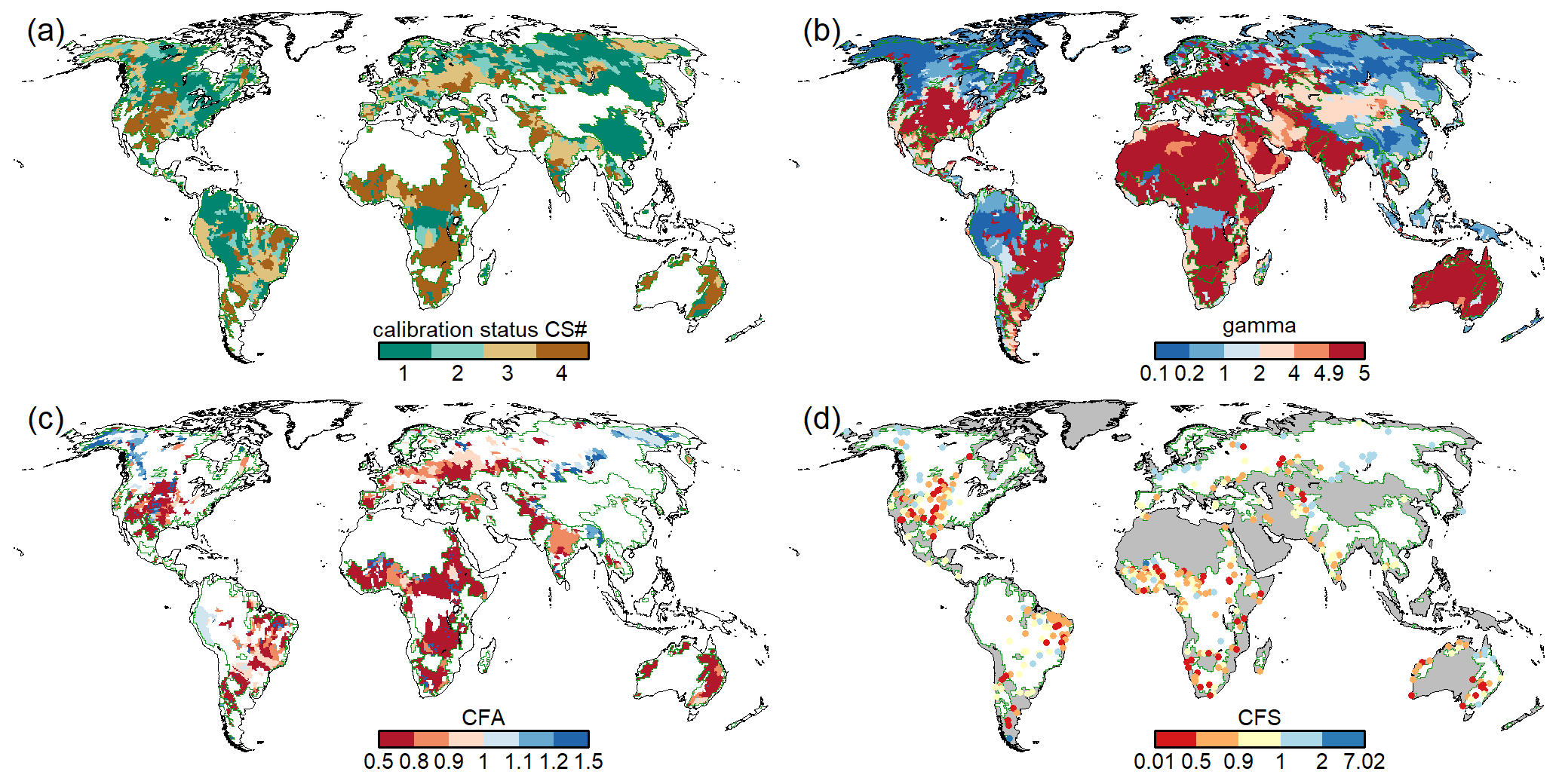
Figure 4Results of the calibration of WaterGAP 2.2d to the standard climate forcing with (a) the calibration status (see Sect. 4.9.1) of each calibration basin, (b) calibration parameter γ, (c) areal correction factor CFA and (d) station correction factor CFS. Grey areas in (d) indicate regions with regionalized calibration parameter γ and for (a)–(d) dark green outlines indicate the boundaries of the calibration basins.
5.1 Data provided at PANGAEA repository
A set of standard model outputs is provided via the data publisher and repository PANGAEA hosted by Alfred Wegener Institute, Helmholtz Center for Polar and Marine Research (AWI), Center for Marine Environmental Sciences and University of Bremen (MARUM), under the Creative Commons Attribution-NonCommercial 4.0 International license (CC-BY-NC-4.0). The data are stored using the network Common Data Form (netCDF) format developed by UCAR/Unidata (Unidata, 2019) and are available at https://doi.pangaea.de/10.1594/PANGAEA.918447.
The available storages and flows are listed in Table 1 and Table 2, respectively. To convert between equivalent water heights (e.w.h.) and volumetric units, the cell-specific continental area used in WaterGAP 2.2d is also provided. The assumed water density is 1 g cm−3. The following additional static data used to produce the storages and flows are available: flow direction (Döll and Lehner, 2002), land cover (Appendix C), location of outflow cells of global lakes and reservoirs/regulated lakes (Sect. 4.6), rooting depth (Sect. 4.4.3), maximum soil water storage (Ss,max), and reservoir commissioning year (Sect. 4.6.3). Additionally, the calibration factors γ, CFA, CFS and the calibration status CS (Sect. 4.9.1) are provided. The netCDF files contain metadata with detailed information regarding characteristics of the data (e.g., whether a storage type contains anomaly or absolute values) and a legend where applicable.
Table 1Standard WaterGAP output variables: water storages. Units are kg m−2 (). Temporal resolution is monthly.
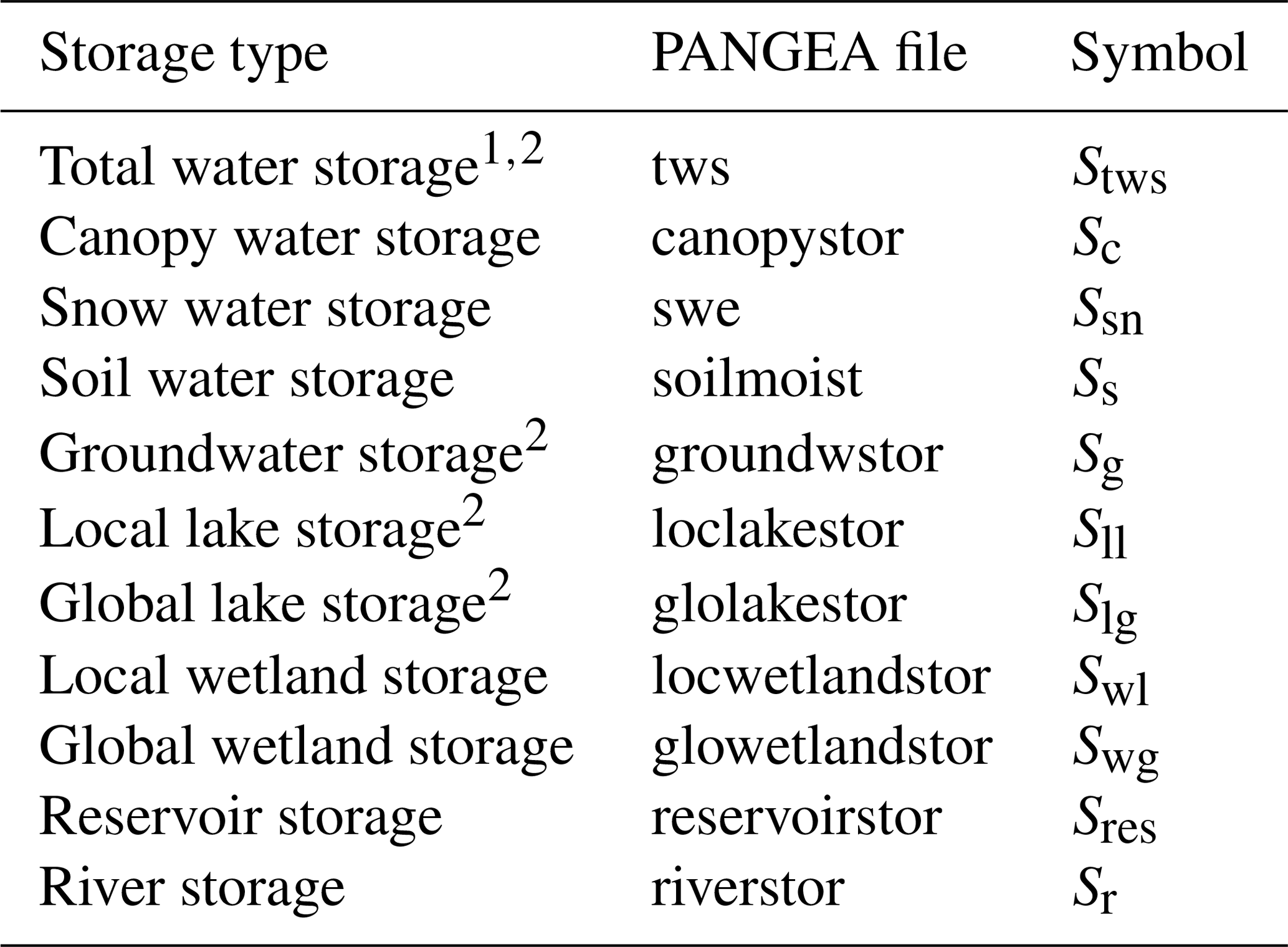
1 Sum of all compartments below. 2 Relative water storages, only anomalies with respect to a reference period can be evaluated.
Table 2Standard WaterGAP output variables: flows. Units are (), except for Qr,out and , which are in m3 s−1. Temporal resolution is monthly.
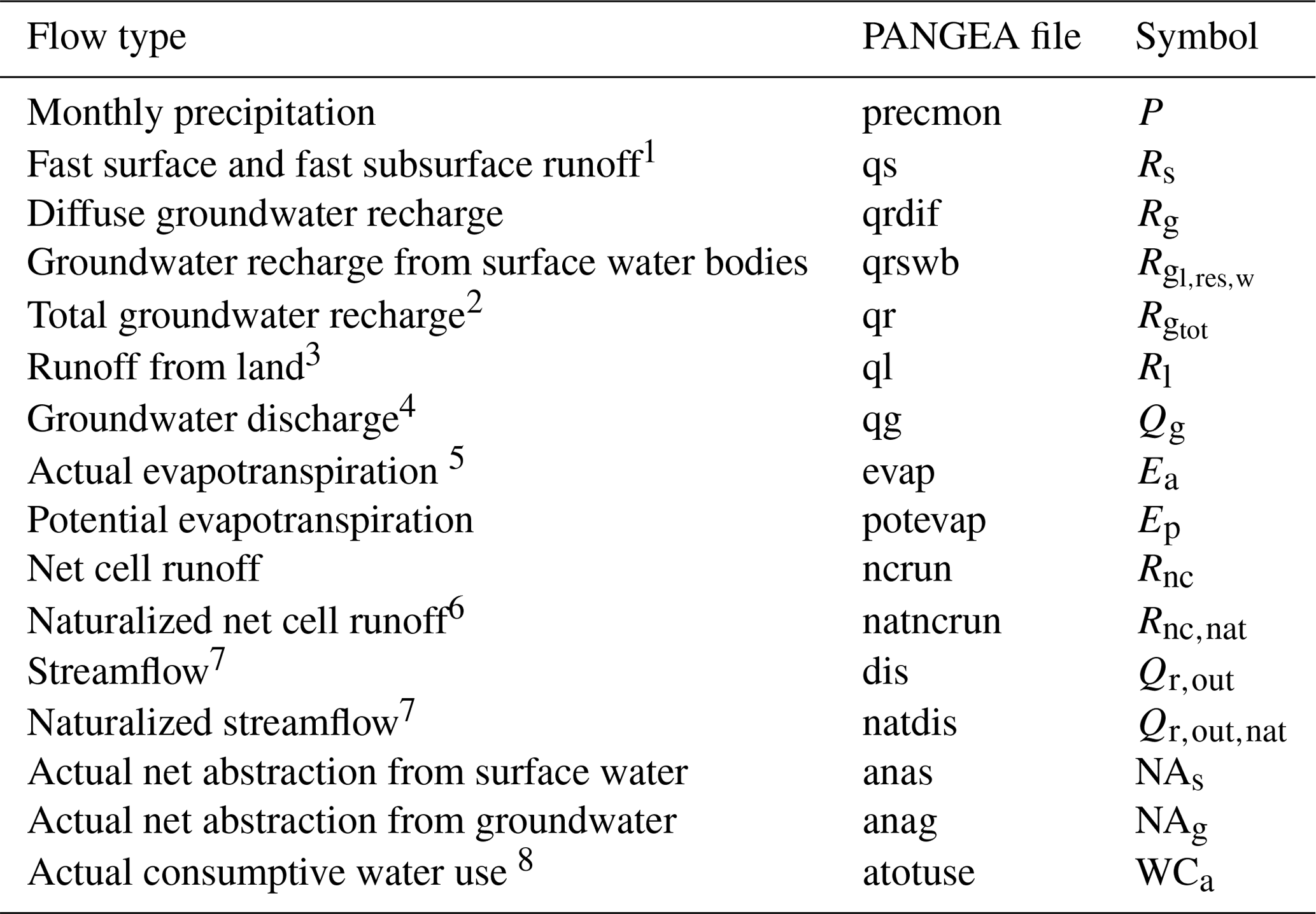
1 Fraction of total runoff from land that does not recharge the groundwater. 2 Sum of qrdif and qrswb. 3 Sum of qs and qrdif. 4 Groundwater runoff. 5 Sum of soil evapotranspiration Es, sublimation Esn, evaporation from canopy Ec, evaporation from water bodies and actual consumptive water use WCa. 6 Equals renewable water resources if averaged over, for example, 30-year time period. 7 River discharge. 8 Sum of anas and anag.
5.2 Caveats in usage of WaterGAP model output
Based on feedback from data users and our own experience, here we describe caveats regarding analysis of specific WaterGAP 2.2d model output with the aim of guiding output users.
-
WaterGAP does not consider leap years. This implies that model output (typically provided in netCDF file format) corresponding to leap years contains the “fill value” instead of a data value at the position of 29 February.
-
The water balance of large lakes and reservoirs is calculated in the outflow cell only. Hence, large numerical values can occur for storages and flows, especially in the case of very large water bodies.
-
In the case that the station correction factor CFS (Sect. 4.9.1) is applied in the grid cell corresponding to the calibration station, multiplication of streamflow by CFS destroys the water balance for this particular grid cell. Hence, the calculation of water balance at various spatial units requires that the amount of reduced/increased streamflow is taken into account in order to close the water balance. A direct inclusion of modified streamflow in, for example, evapotranspiration is not done to avoid physically implausible values for this variable. Water balance is preserved in the case that CFA is used.
-
Gridded model output always relates to the continental area (grid cell area minus ocean area within cell). If flows like runoff from land or diffuse groundwater recharge are simulated to occur only on the land area, i.e., the fraction of the continental area that is not covered by surface water bodies, these flow variables can be small in cells with large water bodies, e.g., groundwater recharge along the Amazon river with riparian wetlands (Fig. 11c).
-
Groundwater recharge below surface water bodies (Eq. 26) can lead to very high values in the case of large surface water bodies and especially in inland sinks that contain large lakes. Temporal changes of this variable can be implausibly high (> 103 mm yr−1).
-
Renewable water resources (Fig. 11a) are defined as the amount of precipitation that is not evapotranspired in the long term (30 years) under naturalized conditions (no water use, no reservoirs). Data users should keep in mind that this variable can only be calculated from naturalized runs and the long-term average of the variable “net cell runoff” Rnc,nat (Table 2). A calculation of renewable water resources using other model setups is not meaningful.
-
Actual consumptive water use can become negative in those cases where water demand is satisfied by spatially distributed grid cells and in the case of irrigation with surface water (see Sect. 4.8).
This section comprises an evaluation of WaterGAP 2.2d using independent data of withdrawal water uses, streamflow and total water storage anomalies (TWSAs) as well as a comparison to the previous model version 2.2 (Müller Schmied et al., 2014).
6.1 Model setup and simulation experiments
In order to compare WaterGAP 2.2d with model version 2.2 (Sect. 6.5), both versions were calibrated and run with the same climate forcing. However, version 2.2 was calibrated using the calibration routine of Müller Schmied et al. (2014). The differences between model versions 2.2 and 2.2d are listed in Appendix A.
A homogenized combination of WATCH Forcing Data based on ERA40 (Weedon et al., 2011) (for 1901–1978) and WATCH Forcing Data methodology applied to ERA-Interim reanalysis (Weedon et al., 2014) (for 1979–2016), with precipitation adjusted to monthly precipitation sums from GPCC (Schneider et al., 2015), was used. The homogenization method is described in Müller Schmied et al. (2016a). The calibrated models have been run for the time period 1901–2016, with a spin-up of 5 years in which the model input for 1901 was used.
6.2 Evaluation datasets
6.2.1 AQUASTAT withdrawal water use data
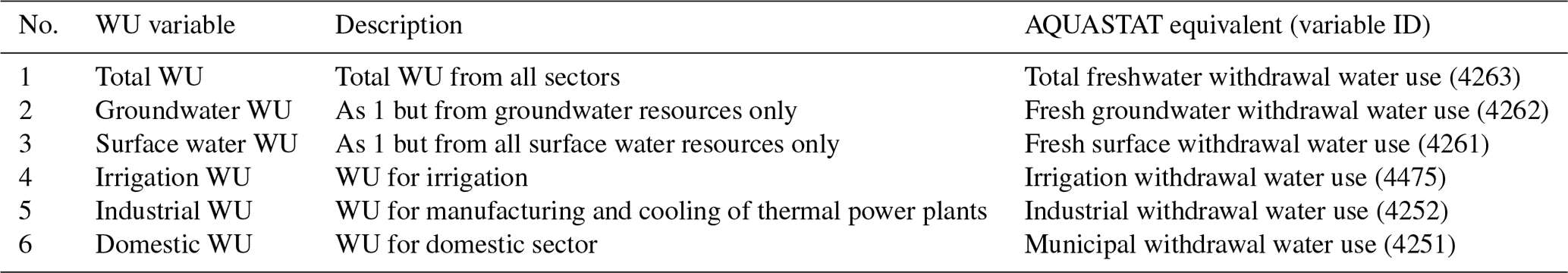
AQUASTAT is the Food and Agriculture Organization of the United Nations Global Information System on Water and Agriculture (FAO, 2019). It contains information on country-level withdrawal water uses for different sectors. These data represent estimates mainly provided by the individual countries. In particular irrigation withdrawal water uses are, for most countries, not based on observations. Six different withdrawal water use variables (Table 3) were available for comparison to WaterGAP 2.2d. For the evaluation, all database entries available on FAO (2019) were used; hence it contains yearly values per country as data units. The evaluation metrics (Sect. 6.3.1) are calculated using each single data point of AQUASTAT without any temporal aggregation by country.
Table 3AQUASTAT variables used for evaluating WaterGAP 2.2d potential withdrawal water use WU, including variable ID reference of AQUASTAT.
6.2.2 GRDC streamflow data
Monthly streamflow time series from 1319 calibration stations from the Global Runoff Data Centre (GRDC) were used for evaluating the performance of WaterGAP 2.2d and 2.2. As the GRDC archive has certain gaps in some regions and times and the calibration objective is to benefit from a maximum of observation data, the typical split-sampling calibration/validation is not appropriate. Even though the same observation data are used for calibration and validation, the validation against monthly time series is meaningful as only long-term mean annual streamflow values have been used for calibration.
6.2.3 GRACE total water storage anomalies
Three mascon solutions of monthly time series of TWSAs from the Gravity Recovery And Climate Experiment (GRACE) satellite mission are considered. The Jet Propulsion Laboratory (JPL) mascon dataset (Watkins et al., 2015; Wiese et al., 2018, 2016) from the GRACE Tellus Website (JPL, 2020) is based on the Level-1 product processed at JPL. A geocenter correction is applied to the degree-1 coefficients following the method from Swenson et al. (2008), the c20 coefficient is replaced with the solutions from satellite laser ranging (SLR; Cheng et al., 2011) and a glacial isostatic adjustment (GIA) correction is applied based on the ICE6G-D model published in Richard Peltier et al. (2018). The Center of Space Research (CSR) RL05 GRACE mascon solution (Save et al., 2016) from the University of Texas website (CSR, 2019) performs the same degree-1 and c20 replacements (but following Cheng et al., 2013) and removes the GIA signal based on the model from Geruo et al. (2012). Last, the Goddard Space Flight Center (GSFC) GRACE mascon solutions (Luthcke et al., 2013) from the Geodesy and Geophysics Science Research Portal (NASA, 2020) applies trend corrections for the c21 and s21 coefficients following Wahr et al. (2015) in addition to the degree-1, c20 and GIA corrections described for CSR.
Monthly TWSA values are provided on 0.5∘ × 0.5∘ grid cells for JPL and CSR, while GSFC provides equal area grids with a spatial resolution of around 1 at the Equator. In this study, the grid values are spatially averaged over 143 river basins with a total area of more than 200 000 km2 each, out of the 1319 basins used for calibration. The considered time span for this study is 2003–2015 (full years of data), limited by available monthly solutions from GSFC between January 2003 and July 2016.
6.3 Evaluation metrics
6.3.1 Nash–Sutcliffe efficiency
The Nash–Sutcliffe efficiency metric (NSE) (–) (Nash and Sutcliffe, 1970) is a traditional metric in hydrological modeling. It provides an integrated measure of modeling performance with respect to mean values and variability and is calculated as follows:
where Oi is the observed value (e.g., monthly streamflow), Si is the simulated value and is the mean observed value. The optimal value of NSE is 1. Values below 0 indicate that the mean value of observations is better than the simulation (Nash and Sutcliffe, 1970). For assessing the performance of low values of water abstraction (Sect. 6.4.1), a logarithmic NSE was calculated in addition by applying logarithmic transformation before calculation of the performance indicator.
6.3.2 Kling–Gupta efficiency
The Kling–Gupta efficiency metric (KGE) (Kling et al., 2012; Gupta et al., 2009) transparently combines the evaluation of bias, variability and timing and is calculated (in its 2012 version) as follows:
where KGEr is the correlation coefficient between simulated and observed values (–), an indicator for the timing; KGEb is the ratio of mean values (Eq. 38) (–), an indicator of biases regarding mean values; and KGEg is the ratio of variability (Eq. 39) (–), an indicator for the variability of simulated (S) and observed (O) values.
where μ is mean value, σ is standard deviation and CV is coefficient of variation. The optimal value of KGE is 1.
6.3.3 TWSA-related metrics
For the evaluation of total water storage anomaly performance, the following metrics were used: R2 (coefficient of determination) as the strength of the linear relationship between simulated and observed variables, and the amplitude ratio as the indicator for variability and trends of both GRACE and WaterGAP data. Amplitude and trends were determined by a linear regression for estimating the most dominant temporal components of the GRACE time series. The time series of monthly TWSAs was approximated by a constant a, a linear trend b, and an annual and a semiannual sinusoidal curve as follows:
where r denotes the residuals. The parameters a to f were estimated via least-squares adjustment. The annual amplitude can be computed by , and thus the annual ratio was calculated by .
6.4 Evaluation results
6.4.1 Water withdrawals
The performance of WaterGAP potential withdrawal water uses is generally of reasonable quality (Fig. 5, for a non-logarithmic graph see Fig. S6). The highest agreement in terms of performance indicator is shown for the total withdrawal water uses with both efficiency metrics close to the optimum value. Slightly less agreement is visible for the separation into groundwater withdrawals (underestimation by WaterGAP) and surface water withdrawals (overestimation by WaterGAP). The domestic sectoral withdrawal water uses are best simulated with WaterGAP, followed by the industrial sector. Here, large differences between NSE and logarithmic NSE are visible, indicating that WaterGAP has specific problems in representing the small values and tending to a general overestimation of industrial withdrawal water uses. Comparing simulated industrial water uses from WaterGAP with data of the FAO AQUASTAT database reveals inconsistencies due to overestimation (i.e., for values > 200 km3 yr−1) as well as underestimation (i.e., for small values) (Fig. 5 and Fig. S6). In terms of overestimated values, values for India and Germany dominate the differences in the time intervals 2008–2012 and 2013–2016, respectively. Water withdrawals of 56 km3 yr−1 for the industry sector (including thermoelectric) were assessed by India's National Commission on Integrated Water Resources Development for 2010 (Bhat, 2014). Here AQUASTAT reports 17 km3 yr−1 and WaterGAP simulates 72 km3 yr−1. In the case of Germany, AQUASTATs reports only the water use of the manufacturing sector but omits the water abstractions of cooling water for thermal electricity production that is included in the WaterGAP results. The underestimation of industrial water uses > 200 km3 yr−1 (Fig. S6) is particularly biased by the reported numbers from the US statistics. While AQUASTAT data include both freshwater and saline water abstractions from manufacturing, thermoelectric abstractions and mining, WaterGAP only accounts for the freshwater part of the manufacturing and thermoelectric abstractions.
WaterGAP performs reasonably well in the irrigation sector with a slightly better logarithmic NSE metric but with the overall lowest sectoral performance in terms of NSE (no visible direction in under- or overestimation).

6.4.2 Streamflow
The performance of WaterGAP 2.2d in terms of monthly streamflow time series at 1319 gauging stations (Fig. 6) reaches a median NSE (KGE) of 0.52 (0.61). However, NSE values below 0 for 259 stations show that WaterGAP 2.2d cannot reproduce monthly and annual streamflow dynamics in one-fifth of the evaluated basins, although the simulated mean annual streamflow fits to the observations due to the calibration. The median for KGEr of 0.79 indicates a relatively satisfactory simulation of the timing of monthly streamflows both seasonally and interannually. As the model is calibrated to match long-term annual river discharge (Sect. 4.9), the median of the bias measure KGEb is, with a value of 1.01, close to the optimum value. In rare cases, values outside the range of 0.9–1.1 occur as for calibration the individual basins were run for the calibration time period (plus 5 initialization years) while the evaluation run was a global run from 1901 to 2016. In the normal global runs, water demand can be fulfilled from neighboring grid cells while this is not possible in the calibration runs. This partially explains the larger biases also seen in Fig. 8. Streamflow variability is mostly underestimated by WaterGAP 2.2d, and median KGEg is 0.85 (Fig. 6).
When analyzing the spatial distribution of streamflow performance indicators, note that a highly seasonal streamflow regime tends to lead to high NSE and KGEg not due to the quality of the evaluated hydrological model but due to the highly seasonal precipitation input. The global distribution of NSE classes shows a diverse pattern (Fig. 7). Whereas large parts of central Europe, Asia and southern America are simulated reasonably well, the performance in northern America and large parts of Africa is in many cases below a value of 0.5. Based on NSE alone it remains unclear why WaterGAP consistently fails to satisfactorily simulate large parts of the well observed northern American region. Further insights can be gained by assessing the spatial distribution of KGE and its components (Fig. 8). The broad picture of overall KGE (Fig. 8a) is similar to the NSE spatial distribution (Fig. 7). In a large fraction of river basins with low NSE and KGE, the timing is off, with KGEr<0.5. One reason could be the inappropriate modeling of the dynamics of lakes and wetland (mainly in Canada) and of reservoir regulations. As most snow-dominated basins in Alaska, Europe and Asia show a reasonably high KGEr of >0.8, it is not likely that snow dynamics are the dominant cause for low correlations between observed and simulated streamflow. For many other regions (e.g., central Asia and the Nile Basin), streamflow regulations due to reservoirs as well as the timing of water abstractions are most likely to cause low performance in timing. The indicator of variability KGEg shows a medium to strong underestimation of streamflow variability in most of the northern snow-dominated basins. Underestimation in the Amazon basin is caused by the inability of WaterGAP to simulate wetland dynamics there. There are also many gauging stations for which WaterGAP overestimates seasonality, even by more than 50 %. Further research and development is needed for improving the GHMs in this respect (Veldkamp et al., 2018).
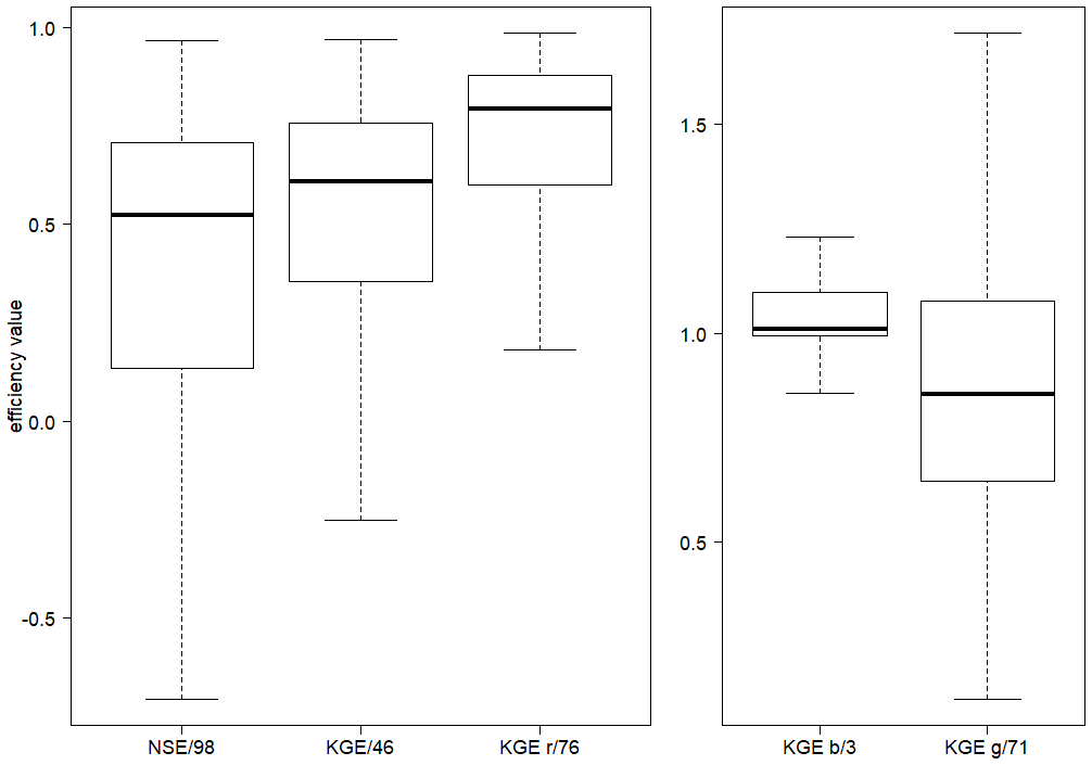
Figure 6Efficiency metrics for monthly streamflow of WaterGAP 2.2d at the 1319 GRDC stations with NSE, KGE and its components. Outliers (outside 1.5× inter-quartile range) are excluded but the number of stations that are defined as outliers are indicated after the metric.

Figure 7Classified NSE efficiency metric for the 1319 river basins in WaterGAP 2.2d.
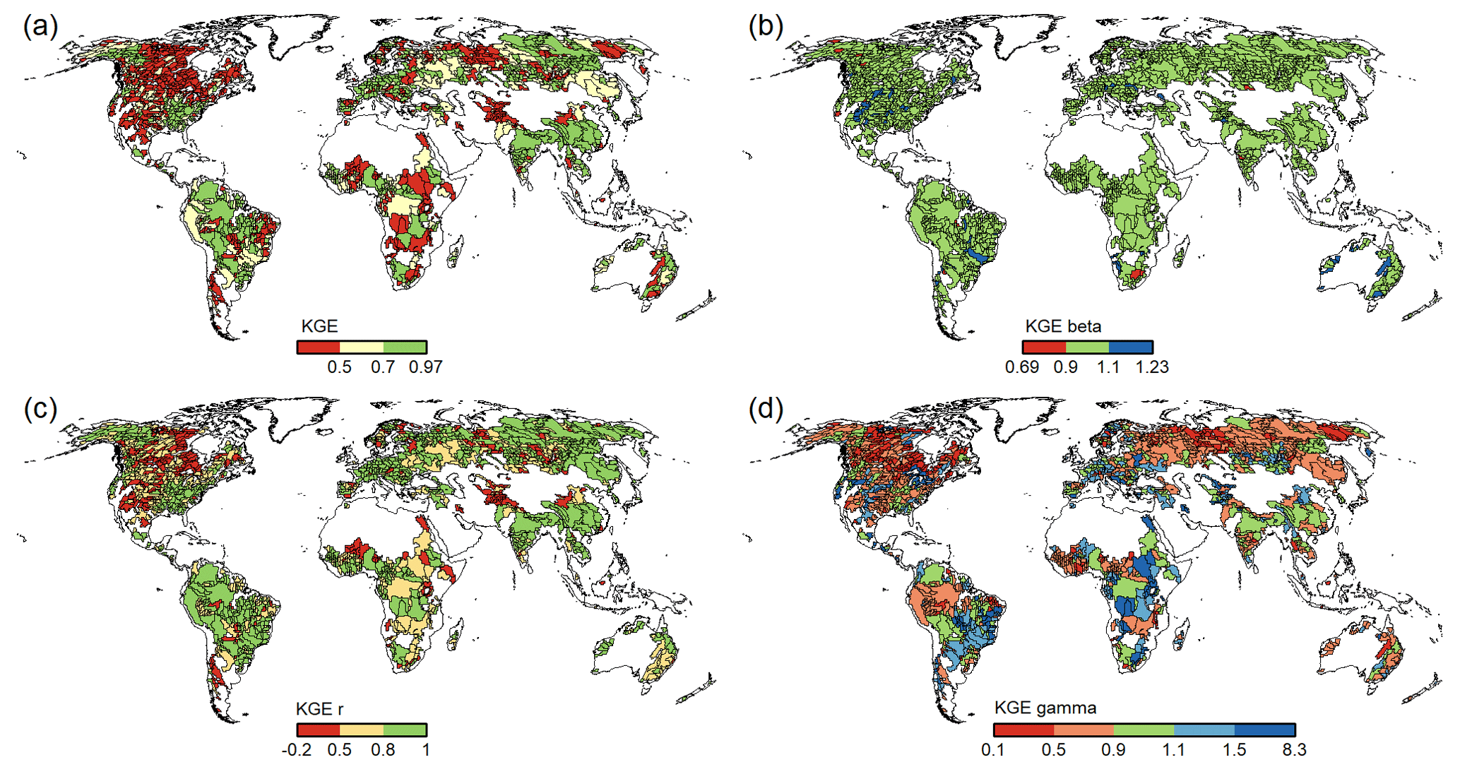
Figure 8Classified KGE efficiency metric and its components for the 1319 river basins in WaterGAP 2.2d.
6.4.3 TWSA
WaterGAP 2.2d underestimates the mean annual TWSA amplitude in 54 % of the 143 investigated river basins by more than 10 % (Fig. 9). Most of these basins are located in Africa, in the northern and monsoon regions of Asia, in Brazil, and in western North America. In contrast, the mean annual amplitude is overestimated in western Russia as well as in eastern and central North America. The correlation coefficient exceeds 0.7 in almost 75 % of the river basins and 0.9 in 22 %. Only 8 % of the basins show a correlation coefficient below 0.5.
The comparison of the TWSA trends shows that GRACE and WaterGAP 2.2d agree in the sign of the trend for 63 % of the 143 basins, for example most European basins; nearly the entire South American continent; and several basins in North America, Asia and Australia, but trends are often underestimated, e.g., in the Amazon and western Russia. Basins with different signs of the trend are scattered around the globe. GRACE suggests strong decreases in water storage in Alaskan basins, which is likely due to glacier mass loss, while WaterGAP determines a small mass increase, likely because WaterGAP does not simulate glaciers. Comparing the spatial pattern of Figs. 9 and 8, no obvious interrelation can be derived between the performances of streamflow and TWSAs.

Figure 9Comparison of basin-average TWSAs of WaterGAP 2.2d and the average values of three GRACE mascon products for 143 basins larger than 200 000 km2, with (a) ratio of amplitude (reddish colors indicate underestimated amplitude of WaterGAP, vice versa for bluish), (b) correlation coefficient, (c) trend of GRACE and (d) trend of WaterGAP 2.2d. All values based on the time series January 2003–December 2015.
6.5 Performance comparison between WaterGAP 2.2d and WaterGAP 2.2
Performance differences are expected due to modifications in model algorithms and the calibration routine (for details on modifications see Appendix A). When comparing the NSE of monthly streamflow (Figs. 7 and S7), the broad picture is similar. WaterGAP 2.2d shows some improvements in northern South America (especially the Amazon) but at the same time gets worse in southern South America. Slight decreases in performance for WaterGAP 2.2d are observed in southern Africa. No major changes are visible in North America, Europe and Asia, with small bidirectional changes. KGE patterns are also relatively similar for both versions (Figs. 8 and S8) and generally follow the differences in NSE. However, there are more regions in Europe and Asia where WaterGAP 2.2d performs better in overall KGE, resulting mainly from an improvement of KGEr. This is also visible in the number of basins per Köppen climate zone, where especially in the tropical A and dry B climates WaterGAP 2.2d has higher performance in KGEr (Table 4). The differences of KGEb are negligible.
KGEg shows significant differences between both model versions, in both directions, but performance of WaterGAP 2.2d is significantly better. Summarizing the basin statistics per Köppen climate zone, 272 instead of only 241 basins are within ±10 % of observed variability in WaterGAP 2.2d in all climate zones except E (Table 5). Fewer river basins (56 % compared to 61 % in 2.2) are subject to an underestimation of streamflow variability. However, the number of basins with overestimation increases slightly from 21 % for WaterGAP 2.2 to 23 % for WaterGAP 2.2d.
The performance of streamflow of the 1319 basins (Fig. S9) is similar for most indicators. The higher variation in KGEb stems from modifications in the calibration routine, where up to ±10 % uncertainty of observed streamflow is allowed. Similarly, the performance statistics of both streamflow and TWSAs (for the 143 basins > 200 000 km2) are very similar for both model versions (Fig. S10).
Table 4Model performance with respect to streamflow timing: number of calibration basins per KGEr category and Köppen–Geiger climate zone.
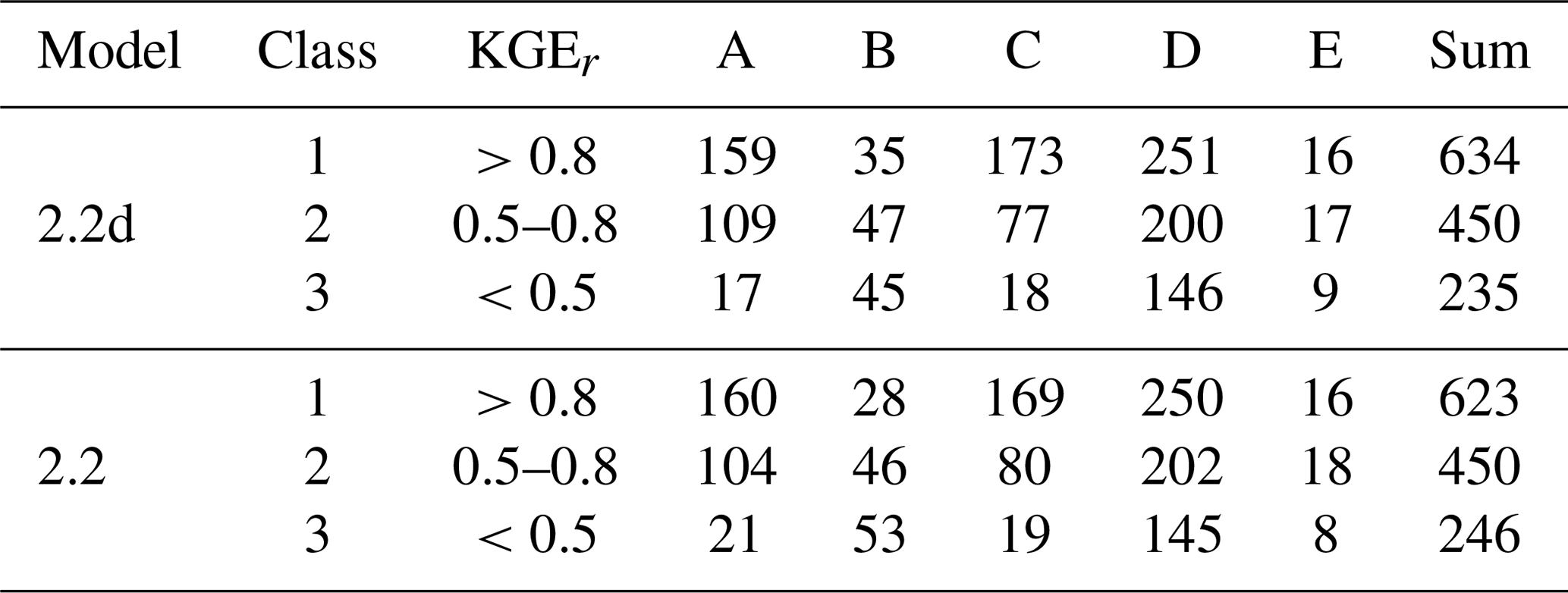
Table 5Model performance with respect to streamflow variability: number of calibration basins per KGEg category and Köppen–Geiger climate zone.
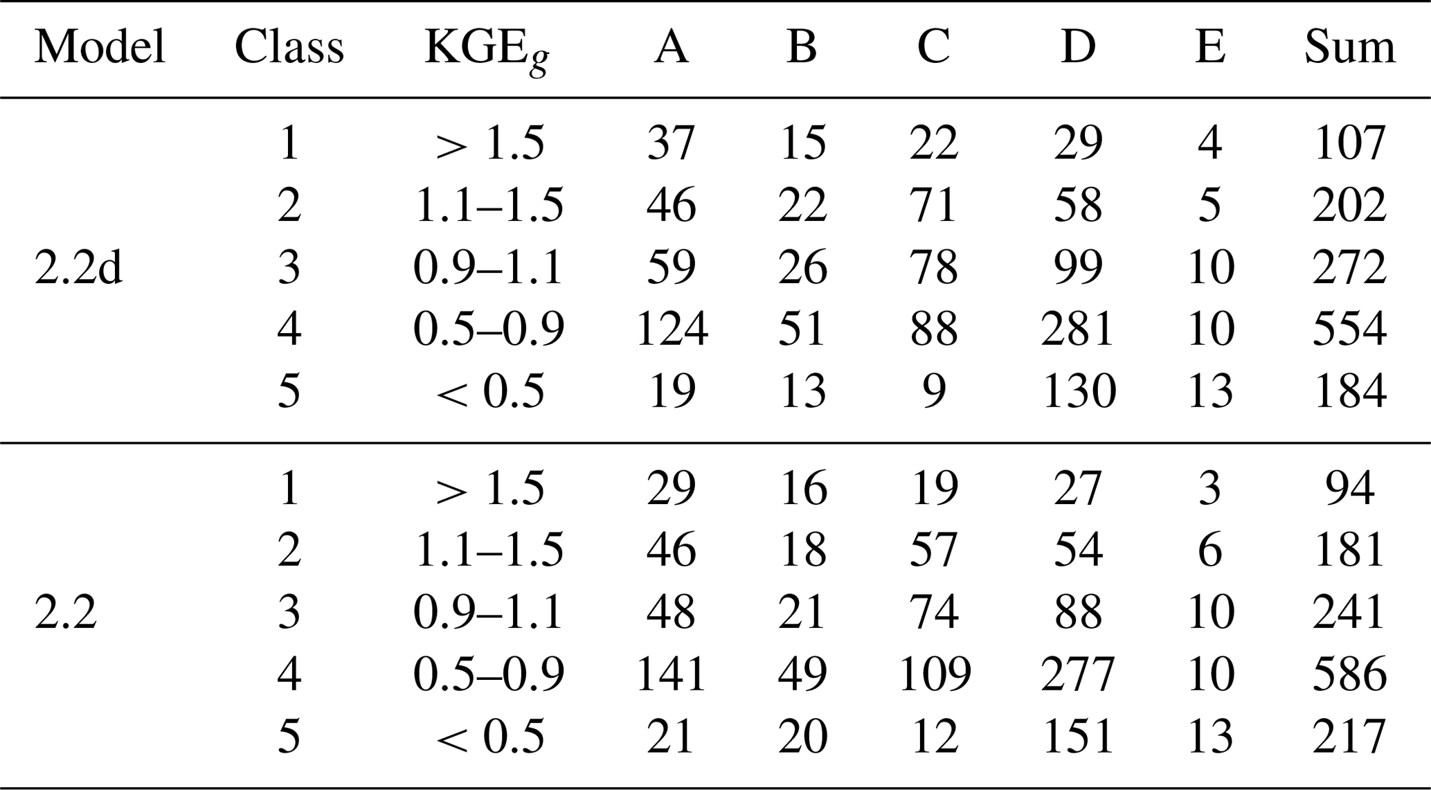
A comparison of simulated seasonality of streamflow and TWSAs in 12 selected large river basins across climate zones shows that performance with respect to both variables are improved in WaterGAP 2.2d for the Lena, Amazon and Yangtze basins (Fig. 10). Simulations for the Congo, Mekong, Mackenzie and Murray basins do not differ. In some basins (Orange, Volga) the simulation of streamflow is improved in WaterGAP 2.2d whereas TWSA seasonality remains similar. In other basins (Rio Parana) seasonality agreement of TWSAs remains the same for WaterGAP 2.2d but streamflow seasonality agreement decreases.
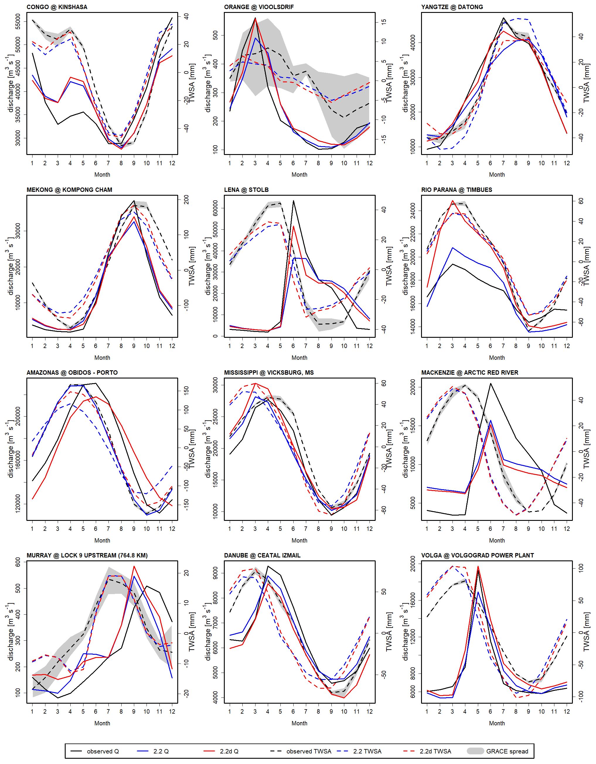
Figure 10Seasonality of streamflow and TWSAs of selected large river basins: model results of WaterGAP 2.2d and WaterGAP 2.2 as well as streamflow and TWSA observations.
This section provides some examples of the WaterGAP 2.2d model applications for characterizing historical freshwater conditions at the global scale.
7.1 Model setup
The model setup is similar to those for the evaluation (Sect. 6.1). For the purpose of model examples, the model was run in both the naturalized (nat) and the anthropogenic (ant) variant (Sect. 4.1).
7.2 Spatial patterns of the global freshwater system
7.2.1 Renewable water resources
The quantification of (total) renewable water resources is one of the key elements of WaterGAP model application. They are defined as the long-term annual difference between precipitation and actual evapotranspiration of a spatial unit, or long-term annual net cell runoff. As runoff and evapotranspiration are influenced by human interference, renewable water resources are calculated based on the naturalized model variant, by averaging Rnc (Sect. 4.7.3) over e.g., a 30-yr time period, resulting in . On around 42.6 % of the global land area (excluding Greenland and Antarctica), total water resources are calculated to be < 100 mm yr−1 during the period 1981–2010, whereas on 19.8 % values are > 500 mm yr−1 (Fig. 11a). Globally averaged renewable water resources are computed to be 307 mm yr−1 or 40 678 km3 yr−1. The global map of inter-annual variability of runoff production (Fig. 11b), here defined as the ratio of runoff in a 1-in-10 dry year to total renewable water resources, shows regions with relatively constant and relatively variable annual runoff generation, in bluish and reddish colors, respectively. High variability is linked with low renewable water resources.
Total renewable water resources include renewable groundwater resources which are the sum of long-term average diffuse groundwater recharge Rg (Fig. 11c) and long-term average point (or focused) groundwater recharge from surface water bodies (Fig. 11d). While focused recharge is the major type of groundwater recharge in some (semi)arid grid cells, its quantification is highly uncertain, and diffuse groundwater recharge dominates in most cells. For 1981–2010, global mean diffuse groundwater recharge is calculated as 111.0 mm yr−1, and global mean focused recharge as 12.8 mm yr−1. Note that as Rg is calculated on (time-variable) land area (continental area minus fraction of lakes, reservoirs, wetlands) but is related to continental area in the standard output (Sect. 5.2), grid cells with large gaining surface water bodies, e.g., wetlands along the Amazon river, show significant lower Rg values than surrounding grid cells.
The sum of diffuse and focused renewable groundwater resources amounts to 40 % of total renewable water resources, highlighting the important contribution of groundwater resources. There have been a number of studies on the potential impact of climate change on renewable groundwater resources (either including or excluding focused recharge), in which WaterGAP was applied as the impact model (Portmann et al., 2013; Döll, 2009; Döll et al., 2018; Herbert and Döll, 2019).
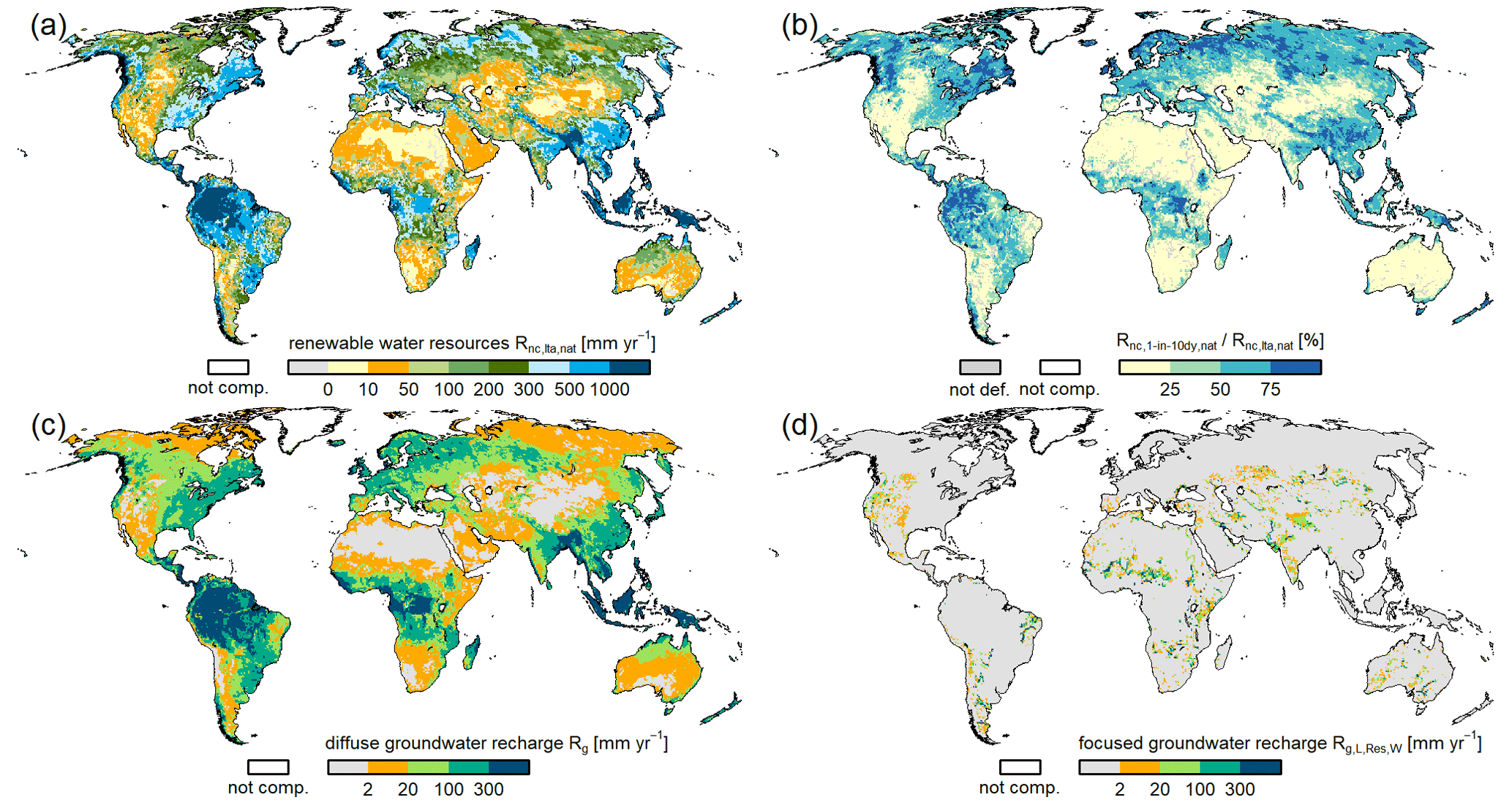
Figure 11Water resources assessment 1981-2010 using WaterGAP 2.2d, with (a) total renewable water resources defined as long-term annual net cell runoff [mm yr−1], (b) 1-in-10 dry-year runoff generation in percent of total renewable water resources [%], (c) long-term annual diffuse groundwater recharge Rg [mm yr−1], (d) long-term annual focused groundwater recharge [mm yr−1]. Results are based on naturalized model runs. In (a) note that negative values for total water resources are possible (Sect. 4.7.3). In (b) areas where the denominator is are labeled as not defined.
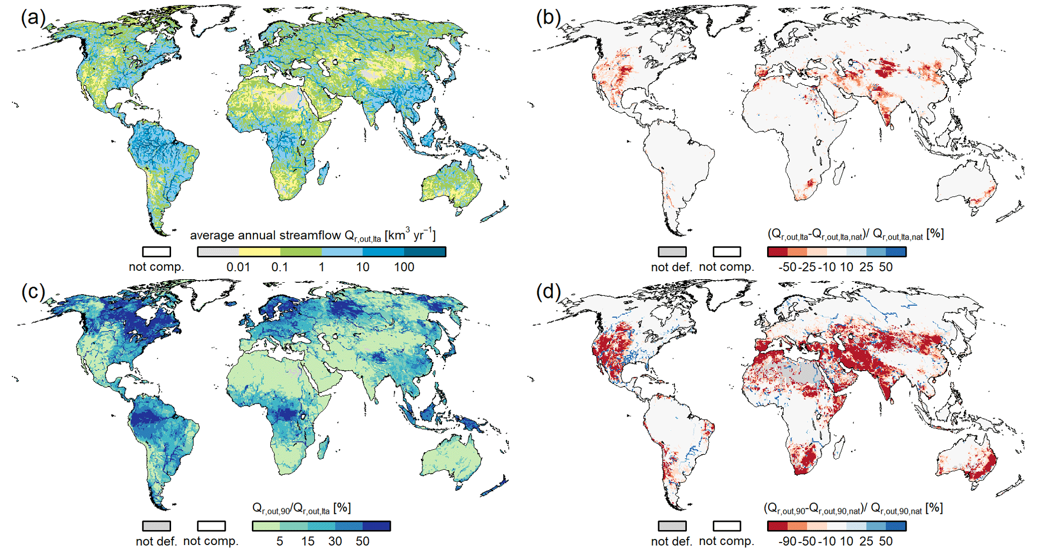
Figure 12Streamflow indicators of WaterGAP 2.2d for 1981–2010 with (a) long-term average annual streamflow (km3 yr−1); (b) indication of streamflow alteration due to human water use and man-made reservoirs, where a reddish color indicates less streamflow for ant conditions, blue the opposite; (c) statistical monthly low flow in percent of ; (d) differences of long-term average statistical monthly low flows as indication of low flow alteration due to human water use and man-made reservoirs. Not defined are areas where the denominator is smaller than 10−5 km3 yr−1.
7.2.2 Streamflow
Streamflow (or river discharge) Qr,out is the model output that integrates all model components and human intervention, routing runoff along the river network. The global map of long-term average annual streamflow under anthropogenic conditions distinctly shows the very high spatial variability of streamflow and very distinctly the large river systems of the Earth (Fig. 12a). Temporal variability of monthly streamflow is much higher in the (semi)arid areas than in humid areas, increasing the spatial discrepancy of streamflow; this can be seen in Fig. 12c, which presents the ratio of the statistical low flow Q90 (the streamflow that is exceeded in 9 out of 10 months) to long-term average annual streamflow. The regions with a ratio of less than 5 % of low flow contribution on average streamflow (the hydrologically highly variable regions) follow in general the definition of (semi)arid grid cells (Fig. B1) with some exceptions such as northern Asia. Different from the spatial pattern of interannual variability of long-term average net cell runoff (Fig. 11b), the spatial pattern of streamflow is characterized by low temporal variability in cells with large rivers, due to the integration of runoff from diverse grid cells as well as large water storage capacities in lakes, reservoirs or wetlands.
The impact of human interventions (human water use and man-made reservoirs) on streamflow is assessed in Fig. 12b for long-term averages and Fig. 12d for the statistical low flow indicator Q90 (please note the different legend for both subfigures). In general, human interventions reduce long-term average streamflow by at least 10 % (50 %) in 11.3 % (1.8 %) of the global land area, mainly due to reduced groundwater discharge to lakes, reservoirs, wetlands and rivers as a consequence of groundwater abstractions, in particular groundwater depletion (compare the red pattern with net abstraction from groundwater in Fig. 15a). There is only a minor share (0.7 %) of global land area, where long-term annual streamflow has been increased by more than 10 % due to human interventions (mainly return flow from groundwater abstractions). The impact of human interventions on Q90 is more pronounced (Fig. 12d). Large reddish patterns (consistent to net abstraction from groundwater in Fig. 15a) indicate the reduction of low flows by at least 10 % (90 %) on 29.7 % (14.4 %) of the global land area. However, there are also bluish river systems visible which represent a global land area of 5.3 % with increase in low flows of more than 10 %. Those areas are located downstream of large reservoirs that due to their storage capacity attenuate the flow regime towards a temporally less variable streamflow. As WaterGAP 2.2d considers only the largest reservoirs with reservoir management algorithm and handles the remaining ∼6000 reservoirs of GRanD as unmanaged water bodies, the impact of streamflow regulation is most likely underestimated.
7.2.3 Water stress
A major motivation for the initial WaterGAP development was to consistently assess water stress on all land areas of the globe (Döll et al., 2003; Alcamo et al., 1998). A common water stress indicator (WSI) is calculated as the ratio of long-term average annual withdrawal water uses (or water abstractions of withdrawal water use) (Sect. 3) and total renewable water resources for different spatial units (e.g., river basins). Renewable water resources in a basin are equal to long-term average naturalized annual streamflow at the outlet of the basin. WSI of 0.2–0.4 is generally assumed to indicate mild water stress and WSI > 0.4 severe water stress (e.g., Greve et al., 2018), while WSI > 1.0 represents a situation where withdrawal water uses are larger than renewable water resources, indicating extreme water scarcity (e.g., Veldkamp et al., 2017). For this example, zero-order river basins (basins that drain to the oceans or inland sinks) were chosen as spatial units (Fig. 13). River basins covering 73.6 % of global land area have a WSI < 0.2 and thus are calculated to have none to only minor water stress. Mild (severe, but below extreme) water stress is represented in river basins that cover 9.7 % (6.9 %) of global land area. Extreme water stress (WSI > 1.0) is simulated in river basins that cover 9.9 % of global land area (red colors in Fig. 13). The spatial pattern of river basins with water stress is similar to the pattern of modification of statistically low flow alteration due to human interventions (Fig. 12d).
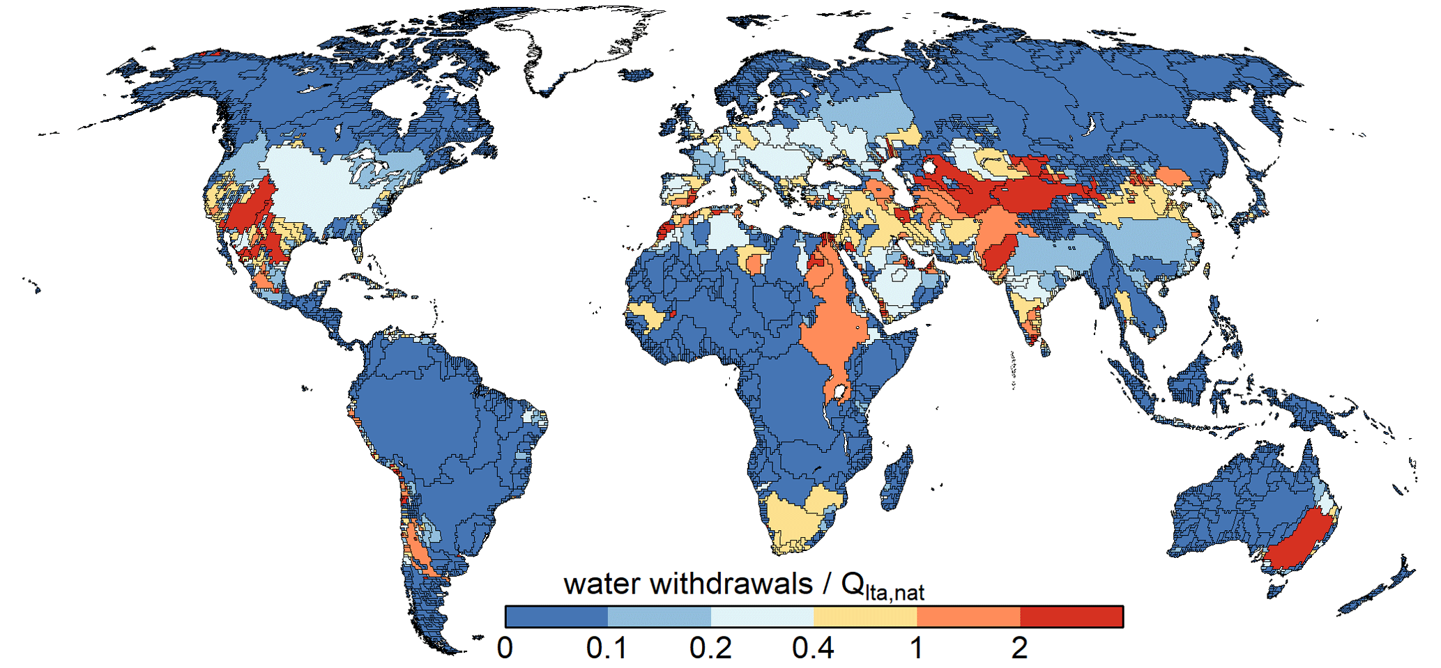
Figure 13Water stress in zero-order river basins for 1981–2010, computed as the ratio of the basin sum of long-term average annual potential total withdrawal water uses (Sect. 3) to long-term average annual streamflow of the basin (i.e., at its outflow cell to the ocean or at its inland sink).
Output of global models is usually shown in the form of two-dimensional planar global maps, which are necessarily distorted. While the Robinson projection that we normally use when presenting WaterGAP results is pleasing to the eye, it does not preserve the actual area of the land surface, and areas closer to Equator are shown relatively smaller than the areas closer to the poles. Using an equal-area projection as in Fig. 14b, Africa is shown larger than in the traditional Robinson maps. For Africa, large blue areas indicate high total renewable water resources per capita. However, very few people live in these large areas. For representing water resources for people instead of on areas, cartograms with population numbers as a distorter can be used (Fig. 14b). In cartograms, map polygons representing spatial units on the Earth's surface are distorted in a way that the units' polygon areas on the map are proportional to a quantitative attribute of the spatial unit (Döll, 2017), here the population in 0.5∘ × 0.5∘ grid cells in 2010. The latter was derived by aggregating 2010 GPWv3 gridded population estimate for the year 2010 (CIESIN, 2016) from its original resolution of 2.5 arcmin. Clearly, with a higher share of red areas, the cartogram indicates a world with less water availability than the “normal” map, and it leads the eye to regions where humans are affected by water scarcity.
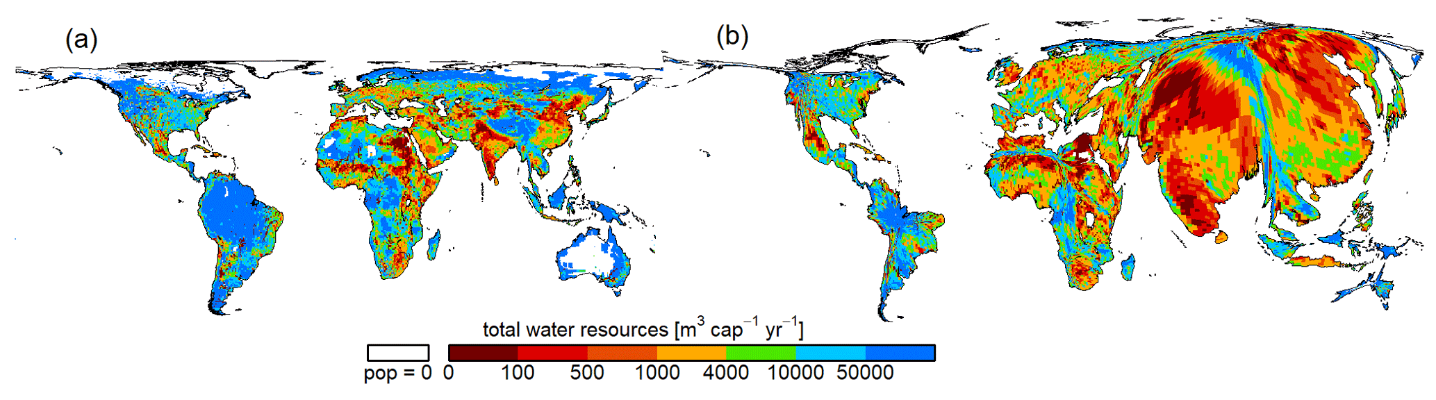
Figure 14Water availability indicator per capita renewable water resources () for 1981–2010 visualized in (a) an equal area projection and (b) as a cartogram with population in 2010 as distorter. In the cartogram each half-degree grid cell is distorted such that its area is proportional to the population of the grid cell.
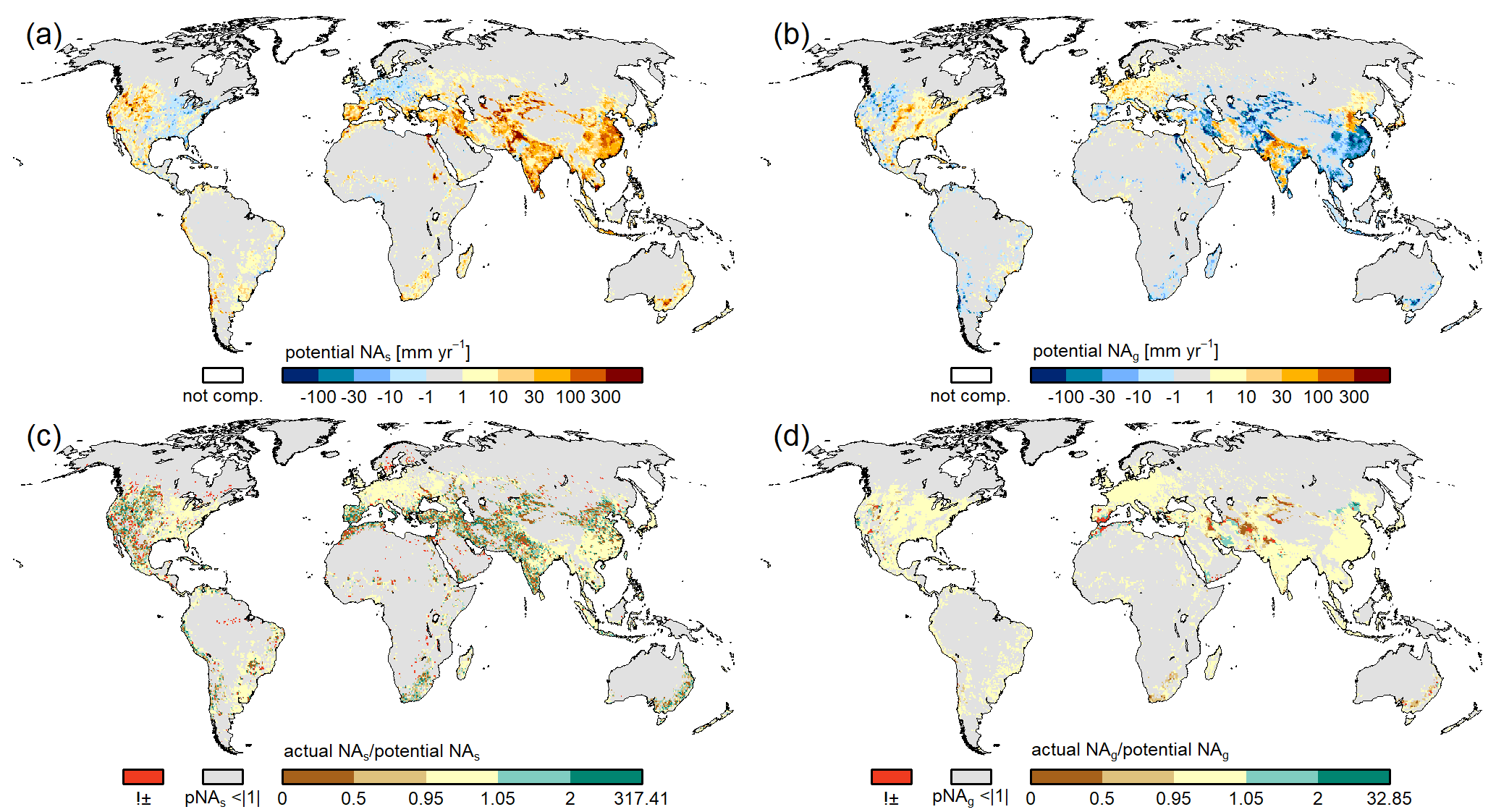
Figure 15Long-term (1981–2010) annual net abstractions: potential net water abstractions from surface water bodies (a), potential net water abstractions from groundwater (b), ratio of actual net water abstractions from surface water bodies to its potential value (c) and ratio of actual net water abstractions from ground water to its potential value. In (a) and (b) negative values indicate a net recharge of surface water and groundwater, respectively, due to return flows caused by human water use, while positive values indicate a net removal of water from the sources. In (c) and (d), cells with potential net water abstractions smaller than mm yr−1 are greyed out. Furthermore, grid cells where the sign of water abstractions changes between potential and actual net abstractions are displayed in red.
7.2.4 Water abstractions
With human water use being essential for the estimation of water stress, quantification of sectoral water uses was a focus already in the initial stages of WaterGAP development (Alcamo et al., 1998). However, a distinction of the sources of water abstractions and the sinks of return flows (groundwater or surface water) was only implemented later, such that potential net abstractions from groundwater and from surface water could be computed (Döll et al., 2012, 2014). Model refinements (see Appendix A2) have lead to a more consistent computation of actual net abstractions from both sources. The general patterns of potential net abstractions (Fig. 15a and b) are consistent with the earlier assessment of Döll et al. (2012). Positive values of NAs and NAg indicate that human water use results in a net subtraction of water from surface water bodies and groundwater, while negative values indicate a man-made addition of water to these water storage compartments. As noted in Sect. 4.8, the actual net abstractions can differ from their potential values. The ratio of actual to potential net surface water abstractions NAs (Fig. 15c) shows a heterogeneous pattern, with adjacent grid cells with values below 0.9 and above 1.1. This is explained by the option to satisfy water demand from a neighboring grid cell. In the case of negative NAs, potential and actual values are always the same, as it is assumed in the model that NAg can always be fulfilled so that return flows to surface water are not changed. There are only a few longer river stretches where actual NAs is smaller than the potential value.
Actual NAg is equal to potential NApot,g except in a few grid cells where potential NApot,s cannot be fulfilled and there is irrigation with surface water (Fig. 15d). In these cells, return flows to groundwater decrease and actual values of NAg increase compared to their potential values. For example, in the case of a positive (negative) potential NAg, a ratio of 1.1 (0.9) means that the difference between actual and potential NAg is 10 % of the absolute value of potential NAg. In most grid cells, actual NAg is equal to the potential value.
Table 6Global-scale (excluding Antarctica and Greenland) water balance components for different time spans as simulated with WaterGAP 2.2d. All units in km3 yr−1. Long-term average volume balance error is calculated as the difference of component 1 and the sum of components 2, 3 and 7.
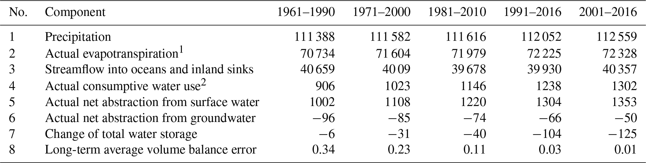
1 Including actual consumptive water use. 2 Sum of rows 5 and 6.
Table 7Globally aggregated (excluding Antarctica and Greenland) water storage component changes during different time periods as simulated by WaterGAP 2.2d. All units in km3 yr−1.

Table 8Globally aggregated (excluding Antarctica and Greenland) sectoral potential withdrawal water use WU and consumptive water use CU (km3 yr−1) as well as use fractions from groundwater (%) as simulated by GWSWUSE of WaterGAP 2.2d for the time period 1991–2016. These values represent demands for water that cannot be completely satisfied in WGHM due to lack of surface water resources (row 5 in Table 6).

7.3 Globally aggregated components of the land water balance components
7.3.1 Major water balance components
Estimation of globally aggregated components of the land water balance components is an intrinsic application field of GHMs. Independent of the time span assessed in Table 6, streamflow into oceans and inland sinks, equivalent to global renewable water resources, amounts to around 40 000 km3 yr−1 (with a range of around 1000 km3 yr−1). Actual evapotranspiration is estimated to be around 71 000 km3 yr−1 (with a range of 1200 km3 yr−1). Renewable water resources estimates are in the range of the estimates of previous WaterGAP model versions and of other global assessments (compare Müller Schmied et al., 2014, their Table 3). Temporal trends of precipitation, actual evapotranspiration and streamflow may not be reliable due to uncertainty of the climate forcing and WaterGAP 2.2d. With less than 10−1 km3 yr−1, the water balance error is negligible (Table 6), which is an improvement compared to earlier model versions (see Müller Schmied et al., 2014, their Table 2).
7.3.2 Water storage components
Total actual consumptive water use has increased over time and reaches the maximum in the most recent time period 2001–2016. The negative value of actual net abstraction from groundwater in Table 6 indicates that, globally aggregated, the groundwater compartment is recharged by return flows from irrigation with surface water (addition of the positive and negative values of NAg in Fig. 15b). A globally averaged anthropogenic increase in groundwater recharge is consistent with a decrease in groundwater storage that is mainly caused by the net groundwater abstractions. The global groundwater storage, however, has decreased (Table 7), mainly due to groundwater depletion in those grid cells where (positive) NAg is higher than groundwater recharge (Döll et al., 2014). The anthropogenic net recharge of groundwater in the grid cells with negative NAg in Fig. 15b does not lead to a substantial increase in groundwater storage but mainly increases groundwater discharge to surface water bodies. The decreasing trend of total water storage is dominated by increasing water storage losses that were balanced in earlier periods by increased water storage in newly constructed reservoirs while dam construction became less during the last three decades (Table 7, Cáceres et al., 2020). However, WaterGAP 2.2d underestimates water storage increases because only the largest reservoirs are simulated as reservoirs including their commissioning year and because the GRanD v1.1 database used in WaterGAP 2.2d does not include some of the major reservoirs that were put into operation after 2000 (Cáceres et al., 2020). Soil water storage also contributes significantly to total water storage changes, showing increases since 1981. Different from what may be expected due to global warming, simulated global snow storage does not decrease over time (Table 7).
7.3.3 Water use components
For the time period 1991–2016, Table 8 presents global sums of annual sectoral potential withdrawal water uses and consumptive water uses as well as the respective fractions that are taken from groundwater (Sect. 3.3). Potential net abstractions from surface water (groundwater) are calculated by GWSWUSE to be 1406 (−153) km3 yr−1 (Sect. 3.3). Actual net abstractions from surface water (groundwater) are computed by WGHM to be 1304 (−66) km3 yr−1 due to restricted surface water availability and consequently less return flows to groundwater from irrigation with surface water. It is thus estimated that 98.8 % of potential consumptive water use of 1253 km3 yr−1 could be fulfilled during 1991–2016, albeit causing groundwater depletion.
A globally consistent quantification of water flows and storages as well as of human water use is needed but challenging, not only due to a lack of observation data but also the difficulty of appropriate process representation in necessarily coarse grid cells (Döll et al., 2016). This study fully describes the state-of-the-art GHM WaterGAP in its newest version 2.2d. Evaluation of model performance using independent data or observations of the key output variables, namely withdrawal water uses, streamflow and total water storage, indicates a reasonable model performance and points to potential areas of model improvement. Model output has been widely used for studying diverse research problems but also for informing the public about the state of the global freshwater system (see Supplement). The description of model algorithms, model outputs and related caveats will allow for better usage of model outputs by other researchers, who can now access these data from the PANGAEA repository.
Ongoing WaterGAP development aims to fully integrate a gradient-based groundwater model (Reinecke et al., 2019), improve the floodplain dynamics of large river basins (e.g., the Amazon) as proposed by Adam (2017) and integrate glacier mass data (Cáceres et al., 2020). In addition, an update of the data basis for water use computations is planned. To enhance cross-sectoral integration in the framework of ISIMIP, modeling of river water temperature according to Van Beek et al. (2012) and Wanders et al. (2019) will be implemented.
A1 Modifications of water use models compared to WaterGAP 2.2
The modifications of water use models compared to WaterGAP 2.2 were as follows:
-
Deficit irrigation with 70 % of optimal (standard) consumptive irrigation water use was applied in grid cells, which were selected based on Döll et al. (2014) and have (1) groundwater depletion of >5 mm yr−1 over 1989–2009 and (2) a >5 % fraction of mean annual irrigation withdrawal water uses in total withdrawal water uses over 1989–2009 (Sect. 3.3). In WaterGAP 2.2, optimal irrigation allowing the plants to evapotranspirate at 100 % of PET was assumed to be done everywhere.
-
The time series of the Historical Irrigation Dataset (HID) for 1900 to 2005 (Siebert et al., 2015) was integrated into the Global Irrigation Model (GIM) (Sect. 3.1) (Portmann, 2017). In WaterGAP 2.2, irrigated areas of the static Global Map of Irrigation Area (GMIA) (Siebert et al., 2005) were scaled by time series of irrigated area per country. In addition to that, the newly available country-specific area actually irrigated (AAI), which is available for 47 countries, was used to update computed ICU until 2010. Version 2.2d enables the cell-specific AAI AEI ratio to be considered (for details see Portmann, 2017).
-
Non-irrigation water uses (domestic, manufacturing) were corrected to plausible values for coastal cells with small continental areas to avoid unrealistically high total water storage values in those cells.
A2 Modifications of WGHM compared to WaterGAP 2.2
A2.1 General
The following general modifications were made:
-
With the introduction of dynamic extents of surface water bodies, land area fractions became variable in time as well (Sect. 2.2).
-
A modified routing approach where water is routed through the storages depends upon the fraction of surface water bodies; otherwise water is routed directly into the river (Sect. 4) (Döll et al., 2014).
-
Since WaterGAP 2.2b, net cell runoff Rnc is the difference between the outflow of a cell and inflow from upstream cells at the end of a time step (Sect. 4.7.3). In the versions before, cell runoff was defined as outflow minus inflow into the river storage.
-
In a modified calibration routine, an uncertainty of 10 % of long-term average river discharge is allowed (following Coxon et al., 2015), meaning that calibration runs in four steps as described in Sect. 4.9.1.
-
Since WaterGAP 2.2b, all model parameters which are potentially used for the calibration/data assimilation integration (including also parameter multiplicators) are read from a text file in JavaScript object notation (JSON) format.
-
The differentiation into semiarid/humid grid cells are defined with a new standard methodology (Appendix B).
-
For WaterGAP 2.2d, the return flows from surface water resources are scaled according to actual NAs (see results in Sect. 7 and Fig. 15). Return flows induced by irrigation from surface water resources were calculated in WaterGAP 2.2 under the assumption that NAs can be fully satisfied. However, this can lead to implausible negative total actual consumptive water use, if surface water availability leads to smaller actual NAs than the return flows.
-
A new storage-based river velocity algorithm was implemented (Sect. 4.7.1).
-
The realization of naturalized runs was improved. In WaterGAP 2.2, reservoirs were treated like global lakes in naturalized runs, while now, global reservoirs are completely removed (but local reservoirs are still handled as local lakes) (Sect. 4.1). Please note that the studies of Döll et al. (2009) and Döll and Zhang (2010) were performed with an even older model version, in which all reservoirs were removed in naturalized runs.
A2.2 Soil
The following modification was made with respect to soil:
A2.3 Groundwater
The following modifications were made with respect to groundwater:
-
Groundwater recharge below surface water bodies (LResWs) is implemented in semiarid and arid regions of Döll et al. (2014) in WaterGAP 2.2d.
-
Regional changes since WaterGAP 2.2b are based on Döll et al. (2014): (1) for Mississippi Embayment Regional Aquifer, groundwater recharge was overestimated, and thus the fraction of runoff from land recharging groundwater was reduced from 80 %–90 % to 10 % in these cells by adapting the groundwater factor fg (Fig. S11); (2) groundwater depletion in the North China Plain was overestimated by a factor of 4, and thus runoff coefficient γ was reduced from 3–5 to 0.1 in this area (Fig. S12); (3) all wetlands in Bangladesh were removed since diffuse groundwater recharge was unrealistically low.
-
In WaterGAP 2.2d and for semiarid/arid grid cells, in the case of less precipitation than 12.5 mm d−1, groundwater recharge remains in the soil column and is not handled as runoff anymore as in the versions before (Sect. 4.4.3).
A2.4 LResWs
The following modifications were made with respect to LResWs:
-
Precipitation on surface water bodies is now also multiplied with the evaporation reduction factor (like evaporation) to keep the water balance consistent (Sect. 4.6.3).
-
Reservoir information was updated, including the year when reservoir began operation (commissioning year; Sect. 4.6.3) (Müller Schmied et al., 2016a; Müller Schmied, 2017).
-
Reservoir commissioning years were implemented in the reservoir algorithm (Sect. 4.6.3) (Müller Schmied et al., 2016a; Müller Schmied, 2017); before this year, the reservoir is not present, and in the case of a regulated lake it is simulated as a global lake. In the versions before 2.2d, reservoirs and regulated lakes are simulated to be always present.
-
For global lakes and reservoirs (where the water balance is calculated in the outflow cell), water demand of all riparian cells is included in the water balance of the outflow cell and thus can be satisfied by global lake or reservoir storage (Sect. 4.6.3).
-
All water storage equations in horizontal water balance are solved analytically in WaterGAP 2.2d (except for local lakes). Those equations now include net abstractions from surface water or groundwater. As a consequence, the sequence of net abstractions has been changed to (1) global lakes, regulated lakes or reservoirs, (2) rivers, and (3) local lakes (Sect. 4.6.3).
-
The areal correction factor (CFA) is included in the water balance of lakes and wetlands in WaterGAP 2.2d (Sect. 4.6.3).
-
In WaterGAP 2.2d (as in versions before WaterGAP 2.2), local and global lake storage can drop to −Smax as described in Hunger and Döll (2008). The area reduction factor (corresponding to the evaporation reduction factor in Hunger and Döll (2008) (their Eq. 1) has been changed accordingly (denominator: 2×Smax). If lake storage S equals Smax, the reduction factor is 1; if S equals −Smax, the reduction factor is 0 (Sect. 4.6.3).
-
Active reservoir storage is no longer assumed to be 85 % but rather 100 % of reported storage (based on comparisons with the literature) (Sect. 4.6.3).
The definition of semiarid and arid grid cells is the basis for fractional routing (Sect. 4.5.3), a groundwater recharge scheme (Sect. 4.4.3, 4.6.3) and a PET equation (Sect. 4.2.3), for example. In the model versions before WaterGAP 2.2c as used in Müller Schmied et al. (2016a), we defined the input file for semiarid/arid or humid grid cells according to the climate forcing used. However, it turned out that this leads to problems when comparing model outputs from different model versions and climate forcings. For example, if well-known non-humid regions (e.g., the High Plains Aquifer and the North China Plain) are classified as humid to a large extent due to uncertain climate forcing (and the approach used), this is not representing reality and can lead to implausible calculation of hydrological processes in those regions. Therefore, a static definition of semiarid/arid and humid grid cells was developed (Fig. B1).
Following Shuttleworth (1993), the Priestley–Taylor α is set to a value of 1.26 for humid regions and of 1.74 for semiarid/arid regions. WaterGAP 2.2c was run with EWEMBI (Lange, 2019) for 1981–2010 with all grid cells defined as humid to avoid predefinition of areas with high or low PET due to the initial setup of the α. Following Middleton and Thomas (1997), drylands were defined based on an aridity index with AI<0.65 and non-drylands with AI≥0.65. Due to the definition of α as a humid value globally, PET might be too low, especially for transitional zones between drylands and non-drylands. Therefore, and based on visual inspection, we defined all grid cells with AI<0.75 as semiarid/arid grid cells. Furthermore, we defined all grid cells north of 55∘ N as humid grid cells.
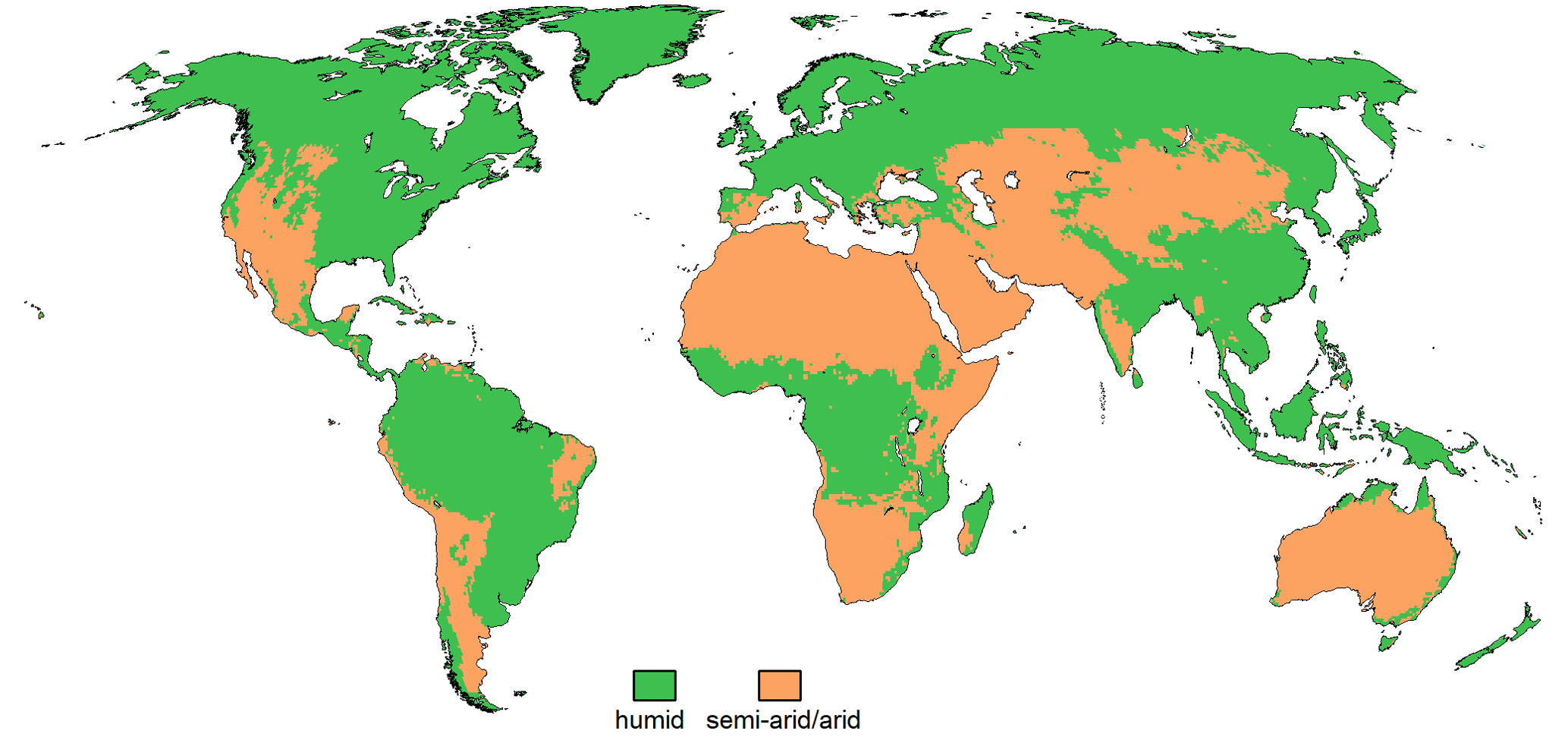
Figure B1Static definition of humid and semiarid/arid grid cells.
WGHM is using a static land cover input map (Fig. C1) which is derived from Moderate Resolution Imaging Spectroradiometer (MODIS, 2020; Friedl et al., 2010) data for the year 2004 (Dörr, 2015). The primary land cover attribute at the original resolution of 500 m is used as a basis. In the case of 500 m MODIS primary land cover being defined as “urban area”, “permanent wetland” or “water body”, the secondary land cover was used instead as those land cover types are included as a separate input (for lakes/wetlands the GLWD dataset, Sect. 4.6; urban areas are implemented as impervious areas, Sect. 4.4.3). Finally, the dominant IGBP (International Geosphere-Biosphere Programme) land cover type (primary land cover) was selected for each 0.5∘ × 0.5∘ grid cell.
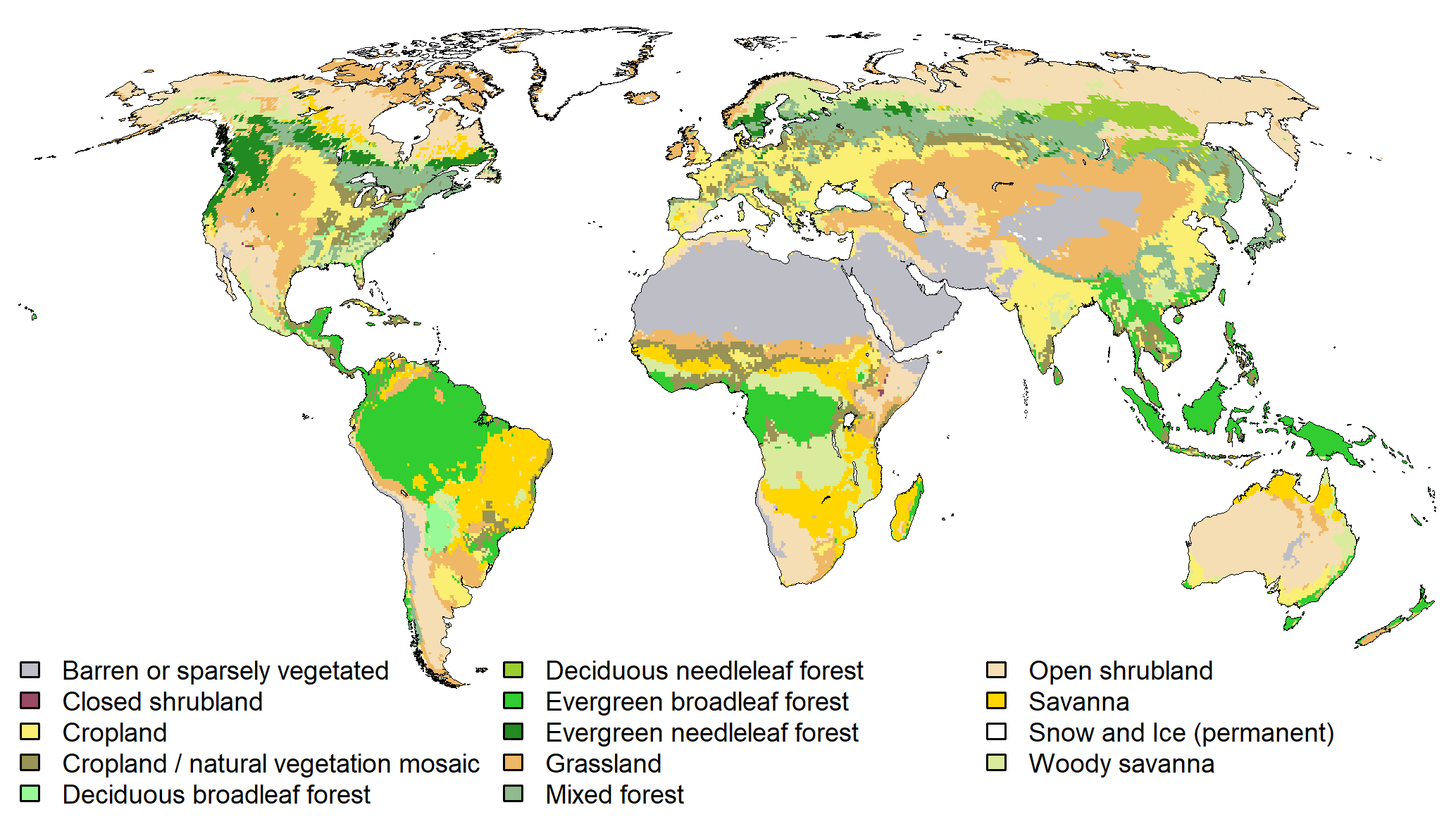
Figure C1Land cover classification of WaterGAP 2.2d.
Table C1Parameters of the leaf area index model from Müller Schmied et al. (2014).
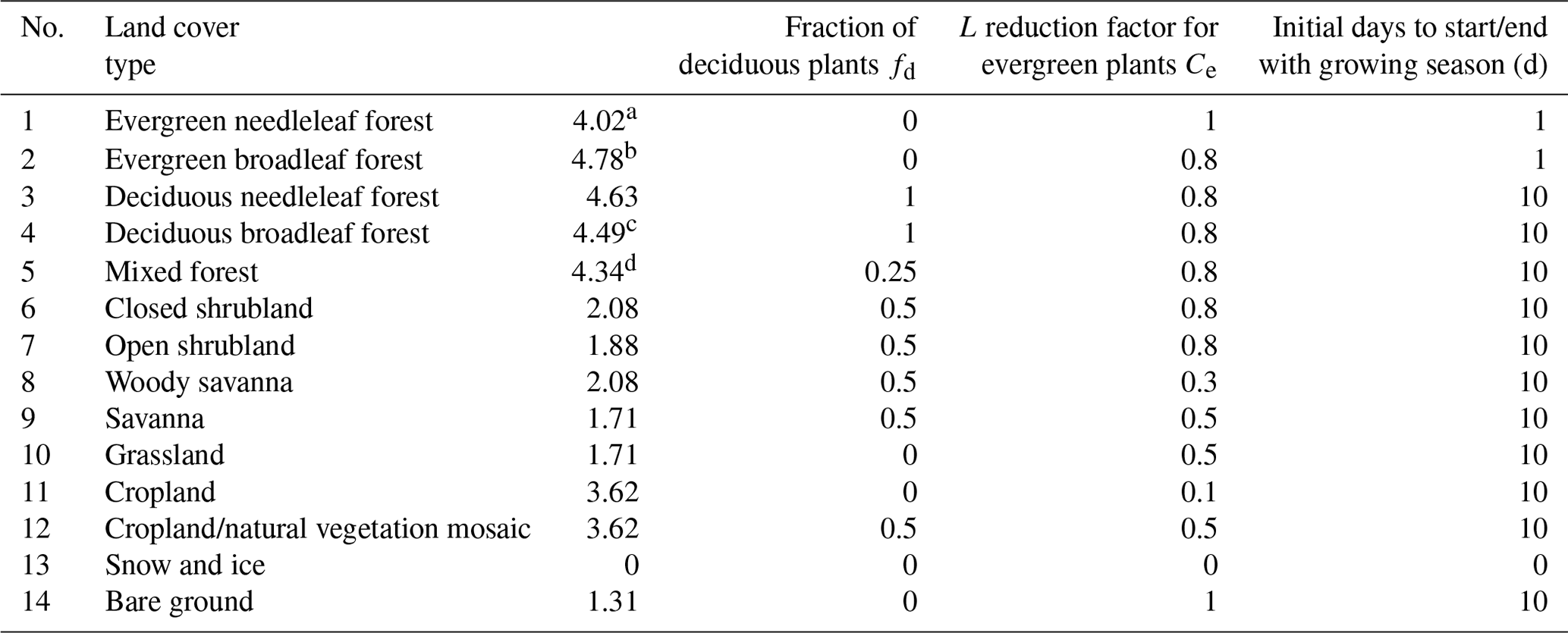
a Lmax is assumed to be the mean value of TeENL and BoENL land cover classes of Scurlock et al. (2001). b Only value for TrEBL and not TeEBL from Scurlock et al. (2001) as in WaterGAP this class is mainly in the tropics. c Mean value from TeDBL and TrDBL from Scurlock et al. (2001). d Mean value of all forest classes. Fraction of deciduous plants and L reduction factor for evergreen plants based on IMAGE (Alcamo et al., 1998) initial days to start/end with growing season are estimated.
Table C2Attributes for IGBP land cover classes used in WaterGAP 2.2d from Müller Schmied et al. (2014). Water has an albedo of 0.08, snow 0.6.
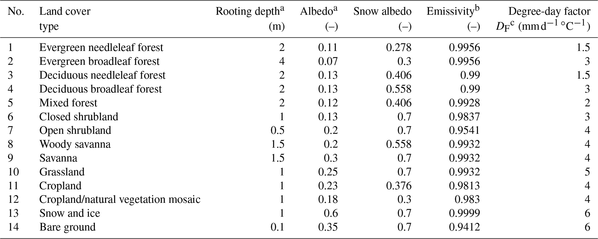
a Adapted from the IMAGE model (Alcamo et al., 1998). b Wilber et al. (1999). c Maniak (1997), WMO (2009).
WGHM uses the Global Lakes and Wetland Database (GLWD) (Lehner and Döll, 2004) and a preliminary but updated version of the Global Reservoir and Dam (GRanD) database (Lehner et al., 2011) to define location, area and other attributes of LResWs. The GLWD database consists of three datasets. GLWD-1 contains shoreline polygons of 3067 large lakes (area is >=50 km2) and 645 large reservoirs (capacity >=0.5 km3); GLWD-2 contains shoreline polygons of approximately 2 500 000 smaller lakes, reservoirs and rivers; and GLWD-3 is a 30 arcsec raster dataset with lakes, reservoirs, rivers and wetland types, including both GLWD-1 and GLWD-2 water bodies. The GRanD v1.1 database includes 6824 reservoir polygons (Lehner et al., 2011). Information from these databases was translated to the six categories of LResWs implemented in WaterGAP and assigned to the 0.5∘ × 0.5∘ grid cells (see Table D1). Figure D1 shows the spatial distribution of the maximum extent of all LResWs (all six categories) in terms of fractional coverage.
Table D1LResW representation in WGHM. The total continental area represented in WaterGAP is 136.782 million km2 (Antarctica is not included in WaterGAP) and 134.396 million km2 without Greenland. The minimum land area (without Greenland), i.e., continental area minus maximum LResW area, is 124.449 million km2.

* Wetland categories of GLWD-3: 4 – freshwater marsh, floodplain, 5 – swamp forest, flooded forest, 7 – pan, brackish/saline wetland, 8 – bog, fen, mire, 10 – 50 %–100 % wetland (using 75 % of area as local wetland), 11 – 25 %–50 % wetland (using 35 % of area as local wetland), 12 – wetland complex (0 %–25 % wetland) (using 15 % of area as local wetland).
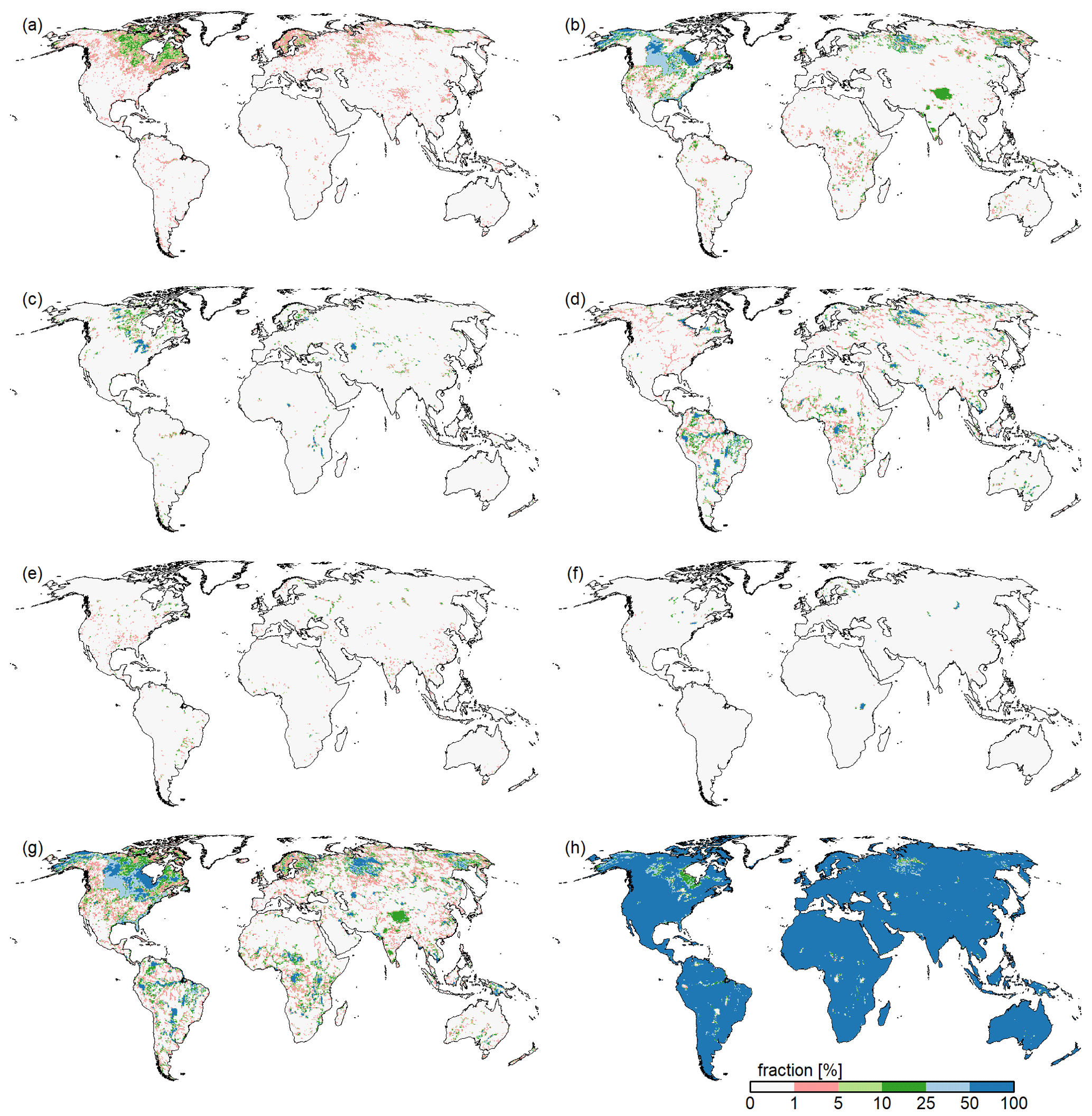
Figure D1Fraction of local lakes (a), local wetlands (b), global lakes (c), global wetlands (d), global reservoirs (e), regulated lakes (f), grid cell area covered by LResWs (represents the maximum extent of LResWs) and land fraction (represents minimum extent of LResWs).
-
Implementation of wetlands. GLWD-3 provides approximately the temporal maximum of wetland extent as wetland outlines were mainly derived from maps and are used to determine Amax. In the case of various input datasets, a wetland was assumed to be present if at least one of the datasets showed one. The wetland types “coastal wetland” (covering 660 000 km2) and “intermittent wetland/lake” (690 000 km2) which are in GLWD-3 are not included in WGHM. Inclusion of coastal wetlands would require the simulation of ocean–land interaction, while intermittent wetlands/lakes of GLWD-3 cover very large parts of the deserts (compare Fig. 5 in Lehner and Döll, 2004) that cannot be assumed to be covered totally by water at any time but rather represent areas where very rarely and at different points in time some parts may be flooded. Rivers shown in GLWD-3 are considered to be (lotic) wetlands and included as wetlands in WGHM. It is assumed that only a river with adjacent wetlands (floodplain) is wide enough to appear as a polygon on the coarse-scale source maps (Lehner and Döll, 2004). For the fractional wetland type “50 %–100 % wetland”, an arbitrary value of 75 % grid cell coverage with wetland is assumed, for “25 %–50 % wetland” a value of 35 % and for “wetland complex” a value of 15 %. The large floodplain wetland of the lower Ganges–Brahmaputra in GLWD-3, covering almost all of Bangladesh, is not simulated as a wetland in WGHM, as during most of the time, only a small part of Bangladesh is inundated.
All wetlands subsumed in fractional classes are assumed to be local, i.e., locally fed. In the case of all other wetland types, global wetlands fed by the whole catchment were identified as follows. All wetland polygons with a direct connection to a major river (as defined by the big_river.shp file available from ESRI) are assumed to receive inflow from a large upstream area and are therefore categorized as global. However, if rivers in this file are categorized as intermittent, the adjacent wetlands are categorized as local in WGHM. All other wetlands are first buffered (to the inside, using a GIS) by a 10 km wide ring such that the outer 10 km of a wetland is considered to be local and the core wetland area inside this buffer ring is considered to be global.
-
Implementation of lakes, man-made reservoirs and regulated lakes. The 0.5∘ × 0.5∘ outflow cell of each global lake is determined based on the GLWD lake polygon and the DDM30 drainage direction map. If more than one global lake has the same outflow cell, the lakes are treated as one lake by adding the lake areas. The same procedure is done in the case of reservoirs/regulated lakes. There are 43 grid cells with 2 reservoirs, 6 grid cells with 3 reservoirs, 2 grid cells with 1 regulated lake and 1 reservoir, 1 grid cell with 2 regulated lakes, and 1 grid cell with 1 global lake and 1 regulated lake. Each cell can be the outflow cell of both a global lake and a global reservoir/regulated lake but if there is a regulated lake and a reservoir in one outflow cell, then they are aggregated. The commissioning year and main purpose of the larger reservoir/regulated lake is used. The commissioning year of the resulting 1109 reservoirs/regulated lakes that are simulated as individual reservoirs/regulated lakes was obtained mainly from the GRanD database but also other sources. In the commissioning year, the reservoir area is increased to its full extent (thus land area fraction is adjusted), the reservoir starts filling and reservoir algorithm is enabled. The storage capacity of the reservoirs which are in operation in the model initialization year is set to the maximum value (Müller Schmied, 2017).
WaterGAP 2.2d is on the way to open source but still in the process of clarifying licensing and copyright issues. Hence, source code cannot be made publicly available but has been available for referees and editors. The standard model output data is available at https://doi.org/10.1594/PANGAEA.918447 (Müller Schmied et al., 2020) and described in Sect. 5. For latest papers published based on WaterGAP 2, we refer to http://www.watergap.de (Döll, 2020).
The supplement related to this article is available online at: https://doi.org/10.5194/gmd-14-1037-2021-supplement.
HMS and PD led the development of WaterGAP 2.2d. HMS led the software development, supported by DC, CH, CN, TAP, EP, FTP, RR, SS, TT, and PD. The paper was conceptualized by HMS and PD. HMS did the calibrations, simulations, data analysis, visualization and model validation, supported by MS regarding validation against GRACE TWS. CN prepared model output for the PANGAEA data repository. The original draft was written by HMS, with specific parts drafted and reviewed by all authors. All authors contributed to the final draft. The revised version was written by HMS, with specific contribution from PD, MF, FTP and DC.
The authors declare that they have no conflict of interest.
We thank Tim Schön for generating Fig. 3 and processing data for Fig. 5 and Hans-Peter Ruhlhof-Döll for processing and generating Fig. 14. We furthermore thank Florian Herz for polishing the reference list and for technical support during manuscript preparation. We are grateful for Edwin Sutanudjaja for providing insights into the withdrawal water use comparison of PCR-GLOBWB. We acknowledge the evaluation datasets from GRDC (The Global Runoff Data Centre, 56068 Koblenz, Germany), AQUASTAT and GRACE (CSR RL05 GRACE mascon solutions were downloaded from http://www2.csr.utexas.edu/grace (last access: 5 March 2020), and JPL GRACE mascon data are available from http://grace.jpl.nasa.gov (last access: 5 March 2020), supported by the NASA MEaSUREs Program). We are grateful for valuable comments and suggestions from one anonymous referee and Gemma Coxon which helped to streamline and improve the consistency of the paper.
The publication of this article was funded by the
Open Access Fund of the Leibniz Association.
This paper was edited by Jeffrey Neal and reviewed by Gemma Coxon and one anonymous referee.
Adam, L.: Modeling water storage dynamics in large floodplains and wetlands, PhD thesis, Goethe-University Frankfurt, 2017. a
Alcamo, J., Leemans, R., and Kreileman, E.: Global Change Scenarios of the 21st Century - Results from the IMAGE 2.1 Model, Pergamon, Oxford, 1998. a, b, c, d
Alcamo, J., Döll, P., Henrichs, T., Kaspar, F., Lehner, B., Rösch, T., and Siebert, S.: Development and testing of the WaterGAP 2 global model of water use and availability, Hydrolog. Sci. J., 48, 317–337, https://doi.org/10.1623/hysj.48.3.317.45290, 2003. a, b
Allen, P. M., Arnold, J. C., and Byars, B. W.: Downstream channel geometry for use in planning level models, J. Am. Water Resour. As., 30, 663–671, https://doi.org/10.1111/j.1752-1688.1994.tb03321.x, 1994. a, b
ArcGIS: Worldmask, available at: https://www.arcgis.com/home/item.html?id=0c667b0505774b8992336dbd9dccb951 (last access: 5 June 2020), 2018. a
Batjes, N.: Development of a world data set of soil water retention properties using pedotransfer rules, Geoderma, 71, 31–52, https://doi.org/10.1016/0016-7061(95)00089-5, 1996. a
Batjes, N. H.: ISRIC-WISE derived soil properties on a 5 by 5 arc-minutes global grid (ver. 1.2), Tech. Rep. 2012/01, ISRIC – World Soil Information, Wageningen, 2012. a, b
Bergström, S.: The HBV model, in: Computer models of watershed hydrology, edited by: Singh, V., Water Resources Publications, Lone Tree, USA, 443–476, 1995. a
Bhat, T. A.: An analysis of demand and supply of water in India, J. Environ. Earth Sci., 4, 67–72, 2014. a
Bierkens, M. F. P., Bell, V. A., Burek, P., Chaney, N., Condon, L. E., David, C. H., de Roo, A., Döll, P., Drost, N., Famiglietti, J. S., Flörke, M., Gochis, D. J., Houser, P., Hut, R., Keune, J., Kollet, S., Maxwell, R. M., Reager, J. T., Samaniego, L., Sudicky, E., Sutanudjaja, E. H., van de Giesen, N., Winsemius, H., and Wood, E. F.: Hyper-resolution global hydrological modelling: what is next? “Everywhere and locally relevant”, Hydrol. Process., 29, 310–320, https://doi.org/10.1002/hyp.10391, 2015. a
Cáceres, D., Marzeion, B., Malles, J. H., Gutknecht, B. D., Müller Schmied, H., and Döll, P.: Assessing global water mass transfers from continents to oceans over the period 1948–2016, Hydrol. Earth Syst. Sci., 24, 4831–4851, https://doi.org/10.5194/hess-24-4831-2020, 2020. a, b, c
Cheng, M., Ries, J. C., and Tapley, B. D.: Variations of the Earth's figure axis from satellite laser ranging and GRACE, J. Geophys. Res.-Sol. Ea., 116, B01409, https://doi.org/10.1029/2010JB000850, 2011. a
Cheng, M., Tapley, B. D., and Ries, J. C.: Deceleration in the Earth's oblateness, J. Geophys. Res.-Sol. Ea., 118, 740–747, https://doi.org/10.1002/jgrb.50058, 2013. a
CIESIN: Gridded population of the world version 3 (GPWv3): Population count, available at: https://sedac.ciesin.columbia.edu/data/collection/gpw-v3 (last acces: 9 February 2021), 2016. a
Coxon, G., Freer, J., Westerberg, I. K., Wagener, T., Woods, R., and Smith, P. J.: A novel framework for discharge uncertainty quantification applied to 500 UK gauging stations, Water Resour. Res., 51, 5531–5546, https://doi.org/10.1002/2014WR016532, 2015. a, b, c, d
CSR: GRACE RL05 mascon solutions, available at: http://www2.csr.utexas.edu/grace/RL05_mascons.html (last access: 5 March 2020), 2019. a
Cucchi, M., Weedon, G. P., Amici, A., Bellouin, N., Lange, S., Müller Schmied, H., Hersbach, H., and Buontempo, C.: WFDE5: bias-adjusted ERA5 reanalysis data for impact studies, Earth Syst. Sci. Data, 12, 2097–2120, https://doi.org/10.5194/essd-12-2097-2020, 2020. a
de Graaf, I. E., van Beek, R. L., Gleeson, T., Moosdorf, N., Schmitz, O., Sutanudjaja, E. H., and Bierkens, M. F.: A global-scale two-layer transient groundwater model: Development and application to groundwater depletion, Adv. Water Resour., 102, 53–67, https://doi.org/10.1016/j.advwatres.2017.01.011, 2017. a
Deardorff, J. W.: Efficient prediction of ground surface temperature and moisture, with inclusion of a layer of vegetation, J. Geophys. Res., 83, 1889, https://doi.org/10.1029/JC083iC04p01889, 1978. a, b
Döll, P.: Vulnerability to the impact of climate change on renewable groundwater resources: a global-scale assessment, Environ. Res. Lett., 4, 035006, https://doi.org/10.1088/1748-9326/4/3/035006, 2009. a
Döll, P.: The WaterGAP Website, available at: http://watergap.de, last access: 25 March 2020. a
Döll, P.: Cartograms facilitate communication of climate change risks and responsibilities, Earths Future, 5, 1182–1195, https://doi.org/10.1002/2017EF000677, 2017. a
Döll, P. and Fiedler, K.: Global-scale modeling of groundwater recharge, Hydrol. Earth Syst. Sci., 12, 863–885, https://doi.org/10.5194/hess-12-863-2008, 2008. a, b, c
Döll, P. and Lehner, B.: Validation of a new global 30-min drainage direction map, J. Hydrol., 258, 214–231, https://doi.org/10.1016/S0022-1694(01)00565-0, 2002. a, b, c
Döll, P. and Siebert, S.: Global modeling of irrigation water requirements, Water Resour. Res., 38, 1–10, https://doi.org/10.1029/2001WR000355, 2002. a, b, c, d, e, f
Döll, P. and Zhang, J.: Impact of climate change on freshwater ecosystems: a global-scale analysis of ecologically relevant river flow alterations, Hydrol. Earth Syst. Sci., 14, 783–799, https://doi.org/10.5194/hess-14-783-2010, 2010. a
Döll, P., Kaspar, F., and Lehner, B.: A global hydrological model for deriving water availability indicators: model tuning and validation, J. Hydrol., 270, 105–134, https://doi.org/10.1016/S0022-1694(02)00283-4, 2003. a, b, c, d, e, f
Döll, P., Fiedler, K., and Zhang, J.: Global-scale analysis of river flow alterations due to water withdrawals and reservoirs, Hydrol. Earth Syst. Sci., 13, 2413–2432, https://doi.org/10.5194/hess-13-2413-2009, 2009. a, b, c, d, e, f
Döll, P., Hoffmann-Dobrev, H., Portmann, F., Siebert, S., Eicker, A., Rodell, M., Strassberg, G., and Scanlon, B.: Impact of water withdrawals from groundwater and surface water on continental water storage variations, J. Geodyn., 59–60, 143–156, https://doi.org/10.1016/j.jog.2011.05.001, 2012. a, b, c, d, e, f, g
Döll, P., Müller Schmied, H., Schuh, C., Portmann, F. T., and Eicker, A.: Global-scale assessment of groundwater depletion and related groundwater abstractions: Combining hydrological modeling with information from well observations and GRACE satellites, Water Resour. Res., 50, 5698–5720, https://doi.org/10.1002/2014WR015595, 2014. a, b, c, d, e, f, g, h, i, j, k, l, m, n, o, p, q
Döll, P., Douville, H., Güntner, A., Müller Schmied, H., and Wada, Y.: Modelling freshwater resources at the global scale: Challenges and prospects, Surv. Geophys., 37, 195–221, https://doi.org/10.1007/s10712-015-9343-1, 2016. a, b
Döll, P., Trautmann, T., Gerten, D., Müller Schmied, H., Ostberg, S., Saaed, F., and Schleussner, C. F.: Risks for the global freshwater system at 1.5 ∘C and 2 ∘C global warming, Environ. Res. Lett., 13, 044038, https://doi.org/10.1088/1748-9326/aab792, 2018. a, b
Döll, P., Trautmann, T., Göllner, M., and Müller Schmied, H.: A global-scale analysis of water storage dynamics of inland wetlands: Quantifying the impacts of human water use and man-made reservoirs as well as the unavoidable and avoidable impacts of climate change, Ecohydrology, 13, 1–18, https://doi.org/10.1002/eco.2175, 2020. a, b
Dörr, P.: Einsatz von MODIS-Fernerkundungsdaten zur Verbesserung der Berechnung der aktuellen Evapotranspiration in WaterGAP – Eine Potentialanalyse, PhD thesis, Goethe-University Frankfurt, 2015. a
Dziegielewski, B., Sharma, S., Bik, T., Margono, H., and Yang, X.: Analysis of water use trends in the Unites States: 1950–1995, Special Report 28, Illinois Water Resources Center, University of Illinois, USA, 2002. a
EIA: International Energy Statistics, available at: http://www.eia.gov/cfapps/ipdbproject/IEDIndex3.cfm?tid=2&pid=2&aid=12 (last access: 8 February 2020), 2012. a
Eicker, A., Schumacher, M., Kusche, J., Döll, P., and Müller Schmied, H.: Calibration/data assimilation approach for integrating GRACE data into the WaterGAP global hydrology model (WGHM) using an Ensemble Kalman Filter: First results, Surv. Geophys., 35, 1285–1309, https://doi.org/10.1007/s10712-014-9309-8, 2014. a
Eisner, S.: Comprehensive evaluation of the WaterGAP3 model across climatic, physiographic, and anthropogenic gradients, PhD thesis, Kassel University, 2015. a, b
FAO: AQUASTAT Main Database, available at: http://www.fao.org/nr/water/aquastat/data/query/index.html?lang=en (last access: 5 June 2020), 2016. a
FAO: AQUASTAT, available at: http://www.fao.org/aquastat/en/, last access: 24 September 2019. a, b, c
FAOSTAT: Live Animals and Livestock Primary, available at: http://faostat.fao.org/site/339/default.aspx (last access: 5 June 2020), 2014. a
Flörke, M., Bärlund, I., and Kynast, E.: Will climate change affect the electricity production sector? A European study, J. Water Clim. Change, 3, 44–54, https://doi.org/10.2166/wcc.2012.066, 2012. a
Flörke, M., Kynast, E., Bärlund, I., Eisner, S., Wimmer, F., and Alcamo, J.: Domestic and industrial water uses of the past 60 years as a mirror of socio-economic development: A global simulation study, Global Environ. Chang., 23, 144–156, https://doi.org/10.1016/j.gloenvcha.2012.10.018, 2013. a, b, c, d, e, f, g, h
Flörke, M., Schneider, C., and Mcdonald, R.: Water competition between cities and agriculture driven by climate change and urban growth, Nat. Sustain., 1, 51–58, https://doi.org/10.1038/s41893-017-0006-8, 2018. a
Friedl, M. A., Sulla-Menashe, D., Tan, B., Schneider, A., Ramankutty, N., Sibley, A., and Huang, X.: MODIS Collection 5 global land cover: Algorithm refinements and characterization of new datasets, Remote Sens. Environ., 114, 168–182, https://doi.org/10.1016/j.rse.2009.08.016, 2010. a
Frieler, K., Lange, S., Piontek, F., Reyer, C. P. O., Schewe, J., Warszawski, L., Zhao, F., Chini, L., Denvil, S., Emanuel, K., Geiger, T., Halladay, K., Hurtt, G., Mengel, M., Murakami, D., Ostberg, S., Popp, A., Riva, R., Stevanovic, M., Suzuki, T., Volkholz, J., Burke, E., Ciais, P., Ebi, K., Eddy, T. D., Elliott, J., Galbraith, E., Gosling, S. N., Hattermann, F., Hickler, T., Hinkel, J., Hof, C., Huber, V., Jägermeyr, J., Krysanova, V., Marcé, R., Müller Schmied, H., Mouratiadou, I., Pierson, D., Tittensor, D. P., Vautard, R., van Vliet, M., Biber, M. F., Betts, R. A., Bodirsky, B. L., Deryng, D., Frolking, S., Jones, C. D., Lotze, H. K., Lotze-Campen, H., Sahajpal, R., Thonicke, K., Tian, H., and Yamagata, Y.: Assessing the impacts of 1.5 °C global warming – simulation protocol of the Inter-Sectoral Impact Model Intercomparison Project (ISIMIP2b), Geosci. Model Dev., 10, 4321–4345, https://doi.org/10.5194/gmd-10-4321-2017, 2017. a
Geruo, A., Wahr, J., and Zhong, S.: Computations of the viscoelastic response of a 3-D compressible Earth to surface loading: an application to Glacial Isostatic Adjustment in Antarctica and Canada, Geophys. J. Int., 192, 557–572, https://doi.org/10.1093/gji/ggs030, 2012. a
Goldewijk, K. K., Beusen, A., and Janssen, P.: Long-term dynamic modeling of global population and built-up area in a spatially explicit way: HYDE 3.1, Holocene, 20, 565–573, https://doi.org/10.1177/0959683609356587, 2010. a
Greve, P., Kahil, T., Mochizuki, J., Schinko, T., Satoh, Y., Burek, P., Fischer, G., Tramberend, S., Burtscher, R., Langan, S., and Wada, Y.: Global assessment of water challenges under uncertainty in water scarcity projections, Nat. Sustain., 1, 486–494, https://doi.org/10.1038/s41893-018-0134-9, 2018. a
Gupta, H. V., Kling, H., Yilmaz, K. K., and Martinez, G. F.: Decomposition of the mean squared error and NSE performance criteria: Implications for improving hydrological modelling, J. Hydrol., 377, 80–91, https://doi.org/10.1016/j.jhydrol.2009.08.003, 2009. a
Haddeland, I., Clark, D. B., Franssen, W., Ludwig, F., Voß, F., Arnell, N. W., Bertrand, N., Best, M., Folwell, S., Gerten, D., Gomes, S., Gosling, S. N., Hagemann, S., Hanasaki, N., Harding, R., Heinke, J., Kabat, P., Koirala, S., Oki, T., Polcher, J., Stacke, T., Viterbo, P., Weedon, G. P., and Yeh, P.: Multimodel Estimate of the Global Terrestrial Water Balance: Setup and First Results, J. Hydrometeorol., 12, 869–884, https://doi.org/10.1175/2011JHM1324.1, 2011. a
Hanasaki, N., Kanae, S., and Oki, T.: A reservoir operation scheme for global river routing models, J. Hydrol., 327, 22–41, https://doi.org/10.1016/j.jhydrol.2005.11.011, 2006. a, b, c
Herbert, C. and Döll, P.: Global assessment of current and future groundwater stress with a focus on transboundary aquifers, Water Resour. Res., 55, 4760–4784, https://doi.org/10.1029/2018WR023321, 2019. a
Hersbach, H., Bell, B., Berrisford, P., Hirahara, S., Horányi, A., Muñoz‐Sabater, J., Nicolas, J., Peubey, C., Radu, R., Schepers, D., Simmons, A., Soci, C., Abdalla, S., Abellan, X., Balsamo, G., Bechtold, P., Biavati, G., Bidlot, J., Bonavita, M., Chiara, G., Dahlgren, P., Dee, D., Diamantakis, M., Dragani, R., Flemming, J., Forbes, R., Fuentes, M., Geer, A., Haimberger, L., Healy, S., Hogan, R. J., Hólm, E., Janisková, M., Keeley, S., Laloyaux, P., Lopez, P., Lupu, C., Radnoti, G., Rosnay, P., Rozum, I., Vamborg, F., Villaume, S., and Thépaut, J.: The ERA5 global reanalysis, Q. J. Roy. Meteor. Soc., 146, 1999–2049, https://doi.org/10.1002/qj.3803, 2020. a
Hoff, H., Döll, P., Fader, M., Gerten, D., Hauser, S., and Siebert, S.: Water footprints of cities – indicators for sustainable consumption and production, Hydrol. Earth Syst. Sci., 18, 213–226, https://doi.org/10.5194/hess-18-213-2014, 2014. a, b
Hunger, M. and Döll, P.: Value of river discharge data for global-scale hydrological modeling, Hydrol. Earth Syst. Sci., 12, 841–861, https://doi.org/10.5194/hess-12-841-2008, 2008. a, b, c, d, e, f
JPL: Monthly mass grids – global mascons (JPL RL06v02), available at: https://grace.jpl.nasa.gov/data/get-data/jpl_global_mascons/, last access: 5 June 2020. a
Kaspar, F.: Entwicklung und Unsicherheitsanalyse eines globalen hydrologischen Modells, PhD thesis, Kassel University Press, 2004. a, b, c
Kim, H.: Global soil wetness project phase 3, available at: http://hydro.iis.u-tokyo.ac.jp/GSWP3/index.html (last access: 25 March 2020), 2014. a
Kling, H., Fuchs, M., and Paulin, M.: Runoff conditions in the upper Danube basin under an ensemble of climate change scenarios, J. Hydrol., 424–425, 264–277, https://doi.org/10.1016/j.jhydrol.2012.01.011, 2012. a
Krysanova, V., Donnelly, C., Gelfan, A., Gerten, D., Arheimer, B., Hattermann, F., and Kundzewicz, Z. W.: How the performance of hydrological models relates to credibility of projections under climate change, Hydrol. Sci. J., 63, 696–720, https://doi.org/10.1080/02626667.2018.1446214, 2018. a
Krysanova, V., Zaherpour, J., Didovets, I., Gosling, S. N., Gerten, D., Hanasaki, N., Müller Schmied, H., Pokhrel, Y., Satoh, Y., Tang, Q., and Wada, Y.: How evaluation of global hydrological models can help to improve credibility of river discharge projections under climate change, Climatic Change, 163, 1353–1377, https://doi.org/10.1007/s10584-020-02840-0, 2020. a
Lange, S.: EartH2Observe, WFDEI and ERA-Interim data Merged and Bias-corrected for ISIMIP (EWEMBI), GFZ Data Services, https://doi.org/10.5880/pik.2019.004, 2019. a
Lehner, B. and Döll, P.: Development and validation of a global database of lakes, reservoirs and wetlands, J. Hydrol., 296, 1–22, https://doi.org/10.1016/j.jhydrol.2004.03.028, 2004. a, b, c, d
Lehner, B., Verdin, K., and Jarvis, A.: New global hydrography derived from spaceborne elevation data, Eos T. Am. Geophys. Un., 89, 93, https://doi.org/10.1029/2008EO100001, 2008. a
Lehner, B., Liermann, C. R., Revenga, C., Vörösmarty, C., Fekete, B., Crouzet, P., Döll, P., Endejan, M., Frenken, K., Magome, J., Nilsson, C., Robertson, J. C., Rödel, R., Sindorf, N., and Wisser, D.: High-resolution mapping of the world's reservoirs and dams for sustainable river-flow management, Front. Ecol. Environ., 9, 494–502, https://doi.org/10.1890/100125, 2011. a, b, c
Luthcke, S. B., Sabaka, T., Loomis, B., Arendt, A., McCarthy, J., and Camp, J.: Antarctica, Greenland and Gulf of Alaska land-ice evolution from an iterated GRACE global mascon solution, J. Glaciol., 59, 613–631, https://doi.org/10.3189/2013JoG12J147, 2013. a
Maniak, U.: Hydrologie und Wasserwirtschaft - Eine Einführung für Ingenieure, Springer-Verlag, Berlin, Heidelberg, New York, https://doi.org/10.1007/978-3-662-07829-7, 1997. a
Meza, I., Siebert, S., Döll, P., Kusche, J., Herbert, C., Eyshi Rezaei, E., Nouri, H., Gerdener, H., Popat, E., Frischen, J., Naumann, G., Vogt, J. V., Walz, Y., Sebesvari, Z., and Hagenlocher, M.: Global-scale drought risk assessment for agricultural systems, Nat. Hazards Earth Syst. Sci., 20, 695–712, https://doi.org/10.5194/nhess-20-695-2020, 2020. a
Middleton, N. and Thomas, D.: World Atlas of Desertification, Arnold, London, 1997. a
Mitchell, T. D. and Jones, P. D.: An improved method of constructing a database of monthly climate observations and associated high-resolution grids, Int. J. Clim., 25, 693–712, https://doi.org/10.1002/joc.1181, 2005. a
MODIS: Moderate resolution imaging spectroradiometer, available at: https://modis.gsfc.nasa.gov/, last access: 14 April 2020. a
Müller Schmied, H.: Evaluation, modification and application of a global hydrological model, PhD thesis, Goethe-University Frankfurt, 2017. a, b, c, d, e, f, g
Müller Schmied, H., Eisner, S., Franz, D., Wattenbach, M., Portmann, F. T., Flörke, M., and Döll, P.: Sensitivity of simulated global-scale freshwater fluxes and storages to input data, hydrological model structure, human water use and calibration, Hydrol. Earth Syst. Sci., 18, 3511–3538, https://doi.org/10.5194/hess-18-3511-2014, 2014. a, b, c, d, e, f, g, h, i, j, k, l, m
Müller Schmied, H., Adam, L., Eisner, S., Fink, G., Flörke, M., Kim, H., Oki, T., Portmann, F. T., Reinecke, R., Riedel, C., Song, Q., Zhang, J., and Döll, P.: Variations of global and continental water balance components as impacted by climate forcing uncertainty and human water use, Hydrol. Earth Syst. Sci., 20, 2877–2898, https://doi.org/10.5194/hess-20-2877-2016, 2016a. a, b, c, d, e, f
Müller Schmied, H., Müller, R., Sanchez-Lorenzo, A., Ahrens, B., and Wild, M.: Evaluation of radiation components in a global freshwater model with station-based observations, Water, 8, 450, https://doi.org/10.3390/w8100450, 2016b. a
Müller Schmied, H., Cáceres, D., Eisner, S., Flörke, M., Herbert, C., Niemann, C., Peiris, T. A., Popat, E., Portmann, F. T., Reinecke, R., Shadkam, S., Trautmann, T., and Döll, P.: The global water resources and use model WaterGAP v2.2d – Standard model output, PANGAEA, available at: https://doi.org/10.1594/PANGAEA.918447, 2020. a
NASA: Earth Sciences – Geodesy and Geophysics, available at: https://neptune.gsfc.nasa.gov/gngphys/index.php?section=470, last access: 14 April 2020. a
Nash, J. and Sutcliffe, J.: River flow forecasting through conceptual models part I – A discussion of principles, J. Hydrol., 10, 282–290, https://doi.org/10.1016/0022-1694(70)90255-6, 1970. a, b
Pascolini-Campbell, M. A., Reager, J. T., and Fisher, J. B.: GRACE-based mass conservation as a validation target for basin-scale evapotranspiration in the contiguous united states, Water Resour. Res., 56, e2019WR026594, https://doi.org/10.1029/2019WR026594, 2020. a
Portmann, F. T.: Global irrigation in the 20th century: extension of the WaterGAP Global Irrigation Model (GIM) with the spatially explicit Historical Irrigation Data set (HID), Frankfurt Hydrology Paper, 18, 131 pp., 2017. a, b, c, d
Portmann, F. T., Siebert, S., and Döll, P.: MIRCA2000—Global monthly irrigated and rainfed crop areas around the year 2000: A new high-resolution data set for agricultural and hydrological modeling, Global Biogeochem. Cy., 24, GB1011, https://doi.org/10.1029/2008GB003435, 2010. a
Portmann, F. T., Döll, P., Eisner, S., and Flörke, M.: Impact of climate change on renewable groundwater resources: assessing the benefits of avoided greenhouse gas emissions using selected CMIP5 climate projections, Environ. Res. Lett., 8, 024023, https://doi.org/10.1088/1748-9326/8/2/024023, 2013. a
Reinecke, R., Foglia, L., Mehl, S., Trautmann, T., Cáceres, D., and Döll, P.: Challenges in developing a global gradient-based groundwater model (G3M v1.0) for the integration into a global hydrological model, Geosci. Model Dev., 12, 2401–2418, https://doi.org/10.5194/gmd-12-2401-2019, 2019. a, b
Richard Peltier, W., Argus, D. F., and Drummond, R.: Comment on “An Assessment of the ICE-6G_C (VM5a) Glacial Isostatic Adjustment Model” by Purcell et al., J. Geophys. Res.-Sol. Ea., 123, 2019–2028, https://doi.org/10.1002/2016JB013844, 2018. a
Save, H., Bettadpur, S., and Tapley, B. D.: High-resolution CSR GRACE RL05 mascons, J. Geophys. Res.-Sol. Ea., 121, 7547–7569, https://doi.org/10.1002/2016JB013007, 2016. a
Scanlon, B. R., Zhang, Z., Save, H., Sun, A. Y., Müller Schmied, H., Van Beek, L. P., Wiese, D. N., Wada, Y., Long, D., Reedy, R. C., Longuevergne, L., Döll, P., and Bierkens, M. F.: Global models underestimate large decadal declining and rising water storage trends relative to GRACE satellite data, P. Natl. Acad. Sci. USA, 115, E1080–E1089, https://doi.org/10.1073/pnas.1704665115, 2018. a
Scanlon, B. R., Zhang, Z., Rateb, A., Sun, A., Wiese, D., Save, H., Beaudoing, H., Lo, M. H., Müller Schmied, H., Döll, P., van Beek, R., Swenson, S., Lawrence, D., Croteau, M., and Reedy, R. C.: Tracking Seasonal Fluctuations in Land Water Storage Using Global Models and GRACE Satellites, Geophys. Res. Lett., 46, 5254–5264, https://doi.org/10.1029/2018GL081836, 2019. a
Schaphoff, S., Forkel, M., Müller, C., Knauer, J., von Bloh, W., Gerten, D., Jägermeyr, J., Lucht, W., Rammig, A., Thonicke, K., and Waha, K.: LPJmL4 – a dynamic global vegetation model with managed land – Part 2: Model evaluation, Geosci. Model Dev., 11, 1377–1403, https://doi.org/10.5194/gmd-11-1377-2018, 2018a. a
Schaphoff, S., von Bloh, W., Rammig, A., Thonicke, K., Biemans, H., Forkel, M., Gerten, D., Heinke, J., Jägermeyr, J., Knauer, J., Langerwisch, F., Lucht, W., Müller, C., Rolinski, S., and Waha, K.: LPJmL4 – a dynamic global vegetation model with managed land – Part 1: Model description, Geosci. Model Dev., 11, 1343–1375, https://doi.org/10.5194/gmd-11-1343-2018, 2018b. a
Schewe, J., Gosling, S. N., Reyer, C., Zhao, F., Ciais, P., Elliott, J., Francois, L., Huber, V., Lotze, H. K., Seneviratne, S. I., van Vliet, M. T., Vautard, R., Wada, Y., Breuer, L., Büchner, M., Carozza, D. A., Chang, J., Coll, M., Deryng, D., de Wit, A., Eddy, T. D., Folberth, C., Frieler, K., Friend, A. D., Gerten, D., Gudmundsson, L., Hanasaki, N., Ito, A., Khabarov, N., Kim, H., Lawrence, P., Morfopoulos, C., Müller, C., Müller Schmied, H., Orth, R., Ostberg, S., Pokhrel, Y., Pugh, T. A., Sakurai, G., Satoh, Y., Schmid, E., Stacke, T., Steenbeek, J., Steinkamp, J., Tang, Q., Tian, H., Tittensor, D. P., Volkholz, J., Wang, X., and Warszawski, L.: State-of-the-art global models underestimate impacts from climate extremes, Nat. Commun., 10, 1–14, https://doi.org/10.1038/s41467-019-08745-6, 2019. a
Schneider, C., Flörke, M., Eisner, S., and Voss, F.: Large scale modelling of bankfull flow: An example for Europe, J. Hydrol., 408, 235–245, https://doi.org/10.1016/j.jhydrol.2011.08.004, 2011. a
Schneider, U., Becker, A., Finger, P., Meyer-Christoffer, A., Rudolf, B., and Ziese, M.: GPCC full data monthly product version 7.0 at 0.5∘: Monthly land-surface precipitation from rain-gauges built on GTS-based and historic data, https://doi.org/10.5676/DWD_GPCC/FD_M_V7_050, 2015. a
Schulze, E., Kelliher, F. M., Korner, C., Lloyd, J., and Leuning, R.: Relationships among maximum stomatal conductance, ecosystem surface conductance, carbon assimilation rate, and plant nitrogen nutrition: A global ecology scaling exercise, Annu. Rev. Ecol. Syst., 25, 629–662, https://doi.org/10.1146/annurev.es.25.110194.003213, 1994. a
Schulze, K. and Döll, P.: Neue Ansätze zur Modellierung von Schneeakkumulation und -schmelze im globalen Wassermodell WaterGAP, in: Tagungsband zum 7. Workshop zur großskaligen Modellierung in der Hydrologie, edited by: Ludwig, R., Reichert, D., and Mauser, W., November 2003, 145–154, Kassel University Press, Kassel, 2004. a, b, c
Schulze, K., Hunger, M., and Döll, P.: Simulating river flow velocity on global scale, Adv. Geosci., 5, 133–136, https://doi.org/10.5194/adgeo-5-133-2005, 2005. a
Schumacher, M., Forootan, E., van Dijk, A., Müller Schmied, H., Crosbie, R., Kusche, J., and Döll, P.: Improving drought simulations within the Murray-Darling Basin by combined calibration/assimilation of GRACE data into the WaterGAP Global Hydrology Model, Remote Sens. Environ., 204, 212–228, https://doi.org/10.1016/j.rse.2017.10.029, 2018. a
Scurlock, J. M., Asner, G. P., and Gower, S. T.: Worldwide historical estimates of leaf area index, 1932-2000, Tech. Rep. December, ORNL Oak Ridge National Laboratory (US), Oak Riidge, USA, 2001. a, b, c, d
Sheffield, J., Goteti, G., and Wood, E. F.: Development of a 50-year high-resolution global dataset of meteorological forcings for land surface modeling, J. Climate, 19, 3088–3111, https://doi.org/10.1175/JCLI3790.1, 2006. a
Shiklomanov, L.: World water resources and water use: Present assessment and outlook for 2025, in: World Water Scenarios Analyses, edited by: Rijsberman, F., p. 396, Earthscan Publications, London (Supplemental data on CD-ROM: Shiklomanov, I., World freshwater resources, available from: International Hydrological Programme, UNESCO, Paris, 2000. a
Shuttleworth, W.: Evaporation, in: Handbook of Hydrology, edited by: Maidment, D., McGraw-Hill, New York, 1–4, 1993. a, b, c
Siebert, S., Döll, P., Hoogeveen, J., Faures, J.-M., Frenken, K., and Feick, S.: Development and validation of the global map of irrigation areas, Hydrol. Earth Syst. Sci., 9, 535–547, https://doi.org/10.5194/hess-9-535-2005, 2005. a
Siebert, S., Burke, J., Faures, J. M., Frenken, K., Hoogeveen, J., Döll, P., and Portmann, F. T.: Groundwater use for irrigation – a global inventory, Hydrol. Earth Syst. Sci., 14, 1863–1880, https://doi.org/10.5194/hess-14-1863-2010, 2010. a
Siebert, S., Henrich, V., Frenken, K., and Burke, J.: Update of the digital global map of irrigation areas to version 5., Tech. rep., Institute of Crop Science and Resource Conservation, Bonn, https://doi.org/10.13140/2.1.2660.6728, 2013. a, b
Siebert, S., Kummu, M., Porkka, M., Döll, P., Ramankutty, N., and Scanlon, B. R.: A global data set of the extent of irrigated land from 1900 to 2005, Hydrol. Earth Syst. Sci., 19, 1521–1545, https://doi.org/10.5194/hess-19-1521-2015, 2015. a, b, c, d
Smith, M.: CROPWAT: A computer program for irrigation planning and management, Irrigation and Drainage Paper No. 46, FAO, Rome, 1992. a
Sutanudjaja, E. H., van Beek, R., Wanders, N., Wada, Y., Bosmans, J. H. C., Drost, N., van der Ent, R. J., de Graaf, I. E. M., Hoch, J. M., de Jong, K., Karssenberg, D., López López, P., Peßenteiner, S., Schmitz, O., Straatsma, M. W., Vannametee, E., Wisser, D., and Bierkens, M. F. P.: PCR-GLOBWB 2: a 5 arcmin global hydrological and water resources model, Geosci. Model Dev., 11, 2429–2453, https://doi.org/10.5194/gmd-11-2429-2018, 2018. a
Swenson, S., Chambers, D., and Wahr, J.: Estimating geocenter variations from a combination of GRACE and ocean model output, J. Geophys. Res.-Sol. Ea., 113, B08410, https://doi.org/10.1029/2007JB005338, 2008. a
Telteu, C.-E., Müller Schmied, H., Thiery, W., Leng, G., Burek, P., Liu, X., Boulange, J. E. S., Seaby, L. P., Grillakis, M., Satoh, Y., Rakovec, O., Stacke, T., Chang, J., Wanders, N., Tao, F., Zhai, R., Shah, H. L., Trautmann, T., Mao, G., Koutroulis, A., Pokhrel, Y., Samaniego, L., Wada, Y., Mishra, V., Liu, J., Newland Gosling, S., Schewe, J., and Zhao, F.: Similarities and differences among fifteen global water models in simulating the vertical water balance, EGU General Assembly 2020, Online, 4–8 May 2020, EGU2020-7549, https://doi.org/10.5194/egusphere-egu2020-7549, 2020. a
Telteu, C.-E., Müller Schmied, H., Thiery, W., Leng, G., Burek, P., Liu, X., Boulange, J. E. S., Seaby Andersen, L., Grillakis, M., Gosling, S. N., Satoh, Y., Rakovec, O., Stacke, T., Chang, J., Wanders, N., Shah, H. L., Trautmann, T., Mao, G., Hanasaki, N., Koutroulis, A., Pokhrel, Y., Samaniego, L., Wada, Y., Mishra, V., Liu, J., Döll, P., Zhao, F., Gädeke, A., Rabin, S., and Herz, F.: Understanding each other's models: a standard representation of global water models to support improvement, intercomparison, and communication, Geosci. Model Dev. Discuss. [preprint], https://doi.org/10.5194/gmd-2020-367, in review, 2021. a
UDI: World Electric Power Plants Database, available at: http://www.platts.com (last access: 5 June 2020), 2004. a
UNEP: The Environmental Data Explorer, as compiled from United Nations Population Division, available at: http://ede.grid.unep.ch, last access: 5 June 2015. a
Unidata: Network common data form (netCDF) version 4, https://doi.org/10.5065/D6H70CW6, 2019. a
U.S. Geological Survey: USGS EROS archive – digital elevation – global 30 arc-second elevation (GTOPO30), available at: https://www.usgs.gov/centers/eros/science/usgs-eros-archive-digital-elevation-global-30-arc-second-elevation-gtopo30?qt-science_center_objects=0#qt-science_center_objects (last access: 25 MArch 2020), 1996. a
Van Beek, L. P., Eikelboom, T., Van Vliet, M. T., and Bierkens, M. F.: A physically based model of global freshwater surface temperature, Water Resour. Res., 48, W09530, https://doi.org/10.1029/2012WR011819, 2012. a
Veldkamp, T., Zhao, F., Ward, P., De Moel, H., Aerts, J., Müller Schmied, H., Portmann, F., Masaki, Y., Pokhrel, Y., Liu, X., Satoh, Y., Gerten, D., Gosling, S., Zaherpour, J., and Wada, Y.: Human impact parameterizations in global hydrological models improve estimates of monthly discharges and hydrological extremes: A multi-model validation study, Environ. Res. Lett., 13, 055008, https://doi.org/10.1088/1748-9326/aab96f, 2018. a, b
Veldkamp, T. I. E., Wada, Y., Aerts, J., Döll, P., Gosling, S. N., Liu, J., Masaki, Y., Oki, T., Ostberg, S., Pokhrel, Y., Satoh, Y., Kim, H., and Ward, P. J.: Water scarcity hotspots travel downstream due to human interventions in the 20th and 21st century, Nat. Commun., 8, 15697, https://doi.org/10.1038/ncomms15697, 2017. a, b
Verzano, K., Bärlund, I., Flörke, M., Lehner, B., Kynast, E., Voß, F., and Alcamo, J.: Modeling variable river flow velocity on continental scale: Current situation and climate change impacts in Europe, J. Hydrol., 424–425, 238–251, https://doi.org/10.1016/j.jhydrol.2012.01.005, 2012. a, b, c
Vörösmarty, C. J., Hoekstra, A. Y., Bunn, S. E., Conway, D., and Gupta, J.: Fresh water goes global, Science, 349, 478–479, https://doi.org/10.1126/science.aac6009, 2015. a
Wada, Y., Bierkens, M. F. P., de Roo, A., Dirmeyer, P. A., Famiglietti, J. S., Hanasaki, N., Konar, M., Liu, J., Müller Schmied, H., Oki, T., Pokhrel, Y., Sivapalan, M., Troy, T. J., van Dijk, A. I. J. M., van Emmerik, T., Van Huijgevoort, M. H. J., Van Lanen, H. A. J., Vörösmarty, C. J., Wanders, N., and Wheater, H.: Human–water interface in hydrological modelling: current status and future directions, Hydrol. Earth Syst. Sci., 21, 4169–4193, https://doi.org/10.5194/hess-21-4169-2017, 2017. a
Wahr, J., Nerem, R. S., and Bettadpur, S. V.: The pole tide and its effect on GRACE time-variable gravity measurements: Implications for estimates of surface mass variations, J. Geophys. Res.-Sol. Ea., 120, 4597–4615, https://doi.org/10.1002/2015JB011986, 2015. a
Wanders, N., van Vliet, M. T., Wada, Y., Bierkens, M. F., and van Beek, L. P.: High-resolution global water temperature modeling, Water Resour. Res., 55, 2760–2778, https://doi.org/10.1029/2018WR023250, 2019. a
Wang, F., Polcher, J., Peylin, P., and Bastrikov, V.: Assimilation of river discharge in a land surface model to improve estimates of the continental water cycles, Hydrol. Earth Syst. Sci., 22, 3863–3882, https://doi.org/10.5194/hess-22-3863-2018, 2018. a
Wartenburger, R., Seneviratne, S. I., Hirschi, M., Chang, J., Ciais, P., Deryng, D., Elliott, J., Folberth, C., Gosling, S. N., Gudmundsson, L., Henrot, A.-J., Hickler, T., Ito, A., Khabarov, N., Kim, H., Leng, G., Liu, J., Liu, X., Masaki, Y., Morfopoulos, C., Müller, C., Müller Schmied, H., Nishina, K., Orth, R., Pokhrel, Y., Pugh, T. A. M., Satoh, Y., Schaphoff, S., Schmid, E., Sheffield, J., Stacke, T., Steinkamp, J., Tang, Q., Thiery, W., Wada, Y., Wang, X., Weedon, G. P., Yang, H., and Zhou, T.: Evapotranspiration simulations in ISIMIP2a–Evaluation of spatio-temporal characteristics with a comprehensive ensemble of independent datasets, Environ. Res. Lett., 13, 075001, https://doi.org/10.1088/1748-9326/aac4bb, 2018. a
Watkins, M. M., Wiese, D. N., Yuan, D. N., Boening, C., and Landerer, F. W.: Improved methods for observing Earth's time variable mass distribution with GRACE using spherical cap mascons, J. Geophys. Res.-Sol. Ea., 120, 2648–2671, https://doi.org/10.1002/2014JB011547, 2015. a
Weedon, G. P., Gomes, S., Viterbo, P., Shuttleworth, W. J., Blyth, E., Österle, H., Adam, J. C., Bellouin, N., Boucher, O., and Best, M.: Creation of the WATCH Forcing Data and its use to assess global and regional reference crop evaporation over land during the twentieth century, J. Hydrometeorol., 12, 823–848, https://doi.org/10.1175/2011JHM1369.1, 2011. a, b
Weedon, G. P., Balsamo, G., Bellouin, N., Gomes, S., Best, M. J., and Viterbo, P.: The WFDEI meteorological forcing data set: WATCH Forcing Data methodology applied to ERA-Interim reanalysis data, Water Resour. Res., 50, 7505–7514, https://doi.org/10.1002/2014WR015638, 2014. a, b
Wiese, D. N., Landerer, F. W., and Watkins, M. M.: Quantifying and reducing leakage errors in the JPL RL05M GRACE mascon solution, Water Resour. Res., 52, 7490–7502, https://doi.org/10.1002/2016WR019344, 2016. a
Wiese, D. N., Yuan, D. N., Boening, C., Landerer, F. W., and Watkins, M. M.: JPL GRACE mascon ocean, ice, and hydrology equivalent water height release 06 coastal resolution improvement (CRI) filtered version 1.0, https://doi.org/10.5067/temsc-3mjc6, 2018. a
Wilber, A. C., Kratz, D. P., and Gupta, S. K.: Surface emissivity maps for use in satellite retrievals of longwave radiation, Tech. rep., NASA Langley Technical Report Server, 1999. a
WMO: Guide to hydrological practices, vol. I: Hydrology – from measurement to hydrological information, and vol. II: Management of water resources and application to hydrological practices, WMO, Geneva, 6th Edn., 2009. a
Wood, E. F., Roundy, J. K., Troy, T. J., van Beek, R. L. P. H., Bierkens, M. F. P., Blyth, E., de Roo, A., Döll, P., Ek, M., Famiglietti, J., Gochis, D., van de Giesen, N., Houser, P., Jaffé, P. R., Kollet, S., Lehner, B., Lettenmaier, D. P., Peters-Lidard, C., Sivapalan, M., Sheffield, J., Wade, A., and Whitehead, P.: Hyperresolution global land surface modeling: Meeting a grand challenge for monitoring earth's terrestrial water, Water Resour. Res., 47, W05301, https://doi.org/10.1029/2010WR010090, 2011. a
Zaherpour, J., Gosling, S. N., Mount, N., Müller Schmied, H., Veldkamp, T. I. E., Dankers, R., Eisner, S., Gerten, D., Gudmundsson, L., Haddeland, I., Hanasaki, N., Kim, H., Leng, G., Liu, J., Masaki, Y., Oki, T., Pokhrel, Y., Satoh, Y., Schewe, J., and Wada, Y.: Worldwide evaluation of mean and extreme runoff from six global-scale hydrological models that account for human impacts, Environ. Res. Lett., 13, 065015, https://doi.org/10.1088/1748-9326/aac547, 2018. a
- Abstract
- Introduction
- WaterGAP 2 framework
- WaterGAP water use models
- WaterGAP Global Hydrology Model (WGHM)
- Standard model output
- Model evaluation
- Examples of model application
- Conclusions and outlook
- Appendix A: Description of changes between the model versions 2.2 and 2.2d
- Appendix B: Definition of arid and humid grid cells
- Appendix C: Land cover input
- Appendix D: Integration of GLWD and GRanD data of lakes, reservoirs and wetlands (LResWs) into WGHM
- Code and data availability
- Author contributions
- Competing interests
- Acknowledgements
- Financial support
- Review statement
- References
- Supplement
The requested paper has a corresponding corrigendum published. Please read the corrigendum first before downloading the article.
- Article
(3189 KB) - Full-text XML
- Corrigendum
-
Supplement
(1721 KB) - BibTeX
- EndNote
- Abstract
- Introduction
- WaterGAP 2 framework
- WaterGAP water use models
- WaterGAP Global Hydrology Model (WGHM)
- Standard model output
- Model evaluation
- Examples of model application
- Conclusions and outlook
- Appendix A: Description of changes between the model versions 2.2 and 2.2d
- Appendix B: Definition of arid and humid grid cells
- Appendix C: Land cover input
- Appendix D: Integration of GLWD and GRanD data of lakes, reservoirs and wetlands (LResWs) into WGHM
- Code and data availability
- Author contributions
- Competing interests
- Acknowledgements
- Financial support
- Review statement
- References
- Supplement