Inequality-constrained free-surface evolution in a full Stokes ice flow model (evolve_glacier v1.1)

Like any gravitationally driven flow that is not constrained at the upper surface, glaciers and ice sheets feature a free surface, which becomes a free-boundary problem within simulations. A kinematic boundary condition is often used to describe the evolution of this free surface. However, in the case of glaciers and ice sheets, the naturally occurring constraint that the ice surface elevation (S) cannot fall below the bed topography (B) ($S-B\ge \mathrm{0}$), in combination with a non-zero mass balance rate complicates the matter substantially. We present an open-source numerical simulation framework to simulate the free-surface evolution of glaciers that directly incorporates this natural constraint. It is based on the finite-element software package FEniCS solving the Stokes equations for ice flow and a suitable transport equation, i.e. “kinematic boundary condition”, for the free-surface evolution. The evolution of the free surface is treated as a variational inequality, constrained by the bedrock underlying the glacier or the topography of the surrounding ground. This problem is solved using a “reduced space” method, where a Newton line search is performed on a subset of the problem (Benson and Munson, 2006). Therefore, the “constrained” non-linear problem-solving capabilities of PETSc's (Portable, Extensible Toolkit for Scientific Computation, Balay et al., 2019) SNES (Scalable Non-linear Equations Solver) interface are used. As the constraint is considered in the solving process, this approach does not require any ad hoc post-processing steps to enforce non-negativity of ice thickness and corresponding mass conservation. The simulation framework provides the possibility to divide the computational domain into different subdomains so that individual forms of the relevant equations can be solved for different subdomains all at once. In the presented setup, this is used to distinguish between glacierised and ice-free regions. The option to chose different time discretisations, spatial stabilisation schemes and adaptive mesh refinement make it a versatile tool for glaciological applications.

We present a set of benchmark tests that highlight that the simulation framework is able to reproduce the free-surface evolution of complex geometries under different conditions for which it is mass-conserving and numerically stable. Real-world glacier examples demonstrate high-resolution change in glacier geometry due to fully resolved 3D velocities and spatially variable mass balance rate, whereby realistic glacier recession and advance states can be simulated. Additionally, we provide a thorough analysis of different spatial stabilisation techniques as well as time discretisation methods. We discuss their applicability and suitability for different glaciological applications.

1 Introduction

Free-boundary problems arise naturally in geophysics. For these kind of problems, in addition to the solution function, parts of the domain itself, specifically the free boundary, are also unknown. Gravitationally driven fluid flows common in geophysics (e.g. water, ice, lava) that are not constrained from the above (e.g. White, 2010) are examples of such free-boundary problems. In addition, melting–freezing processes such as the two-phase Stefan problem (e.g Alexiades, 1992) or marine ice sheet grounding line dynamics (e.g. Schoof, 2011; Goldberg et al., 2018) contain free boundaries as well. Many free-boundary problems can be seen and analysed as variational inequalities (e.g. Kinderlehrer and Stampacchia, 1980), where modern numerical methods and software tools facilitate their solution.

In this paper, we focus on the dynamics of ice, modelled as a non-linear viscous gravity-driven flow, which, due to its free-surface nature, forms a free-boundary problem. If the free-surface flow of ice is defined as a variational inequality, the constraint imposed on the free surface by the bedrock topography is incorporated directly, thus sparing the need for ad hoc post-processing of the free boundary to enforce non-negativity of ice thickness (Jouvet and Bueler, 2012; Bueler, 2016a).

Ice dynamics as free-boundary problems have been studied before, although often with a reduced stress balance known as the shallow ice approximation (SIA, Mahaffy, 1976; Hutter, 1983). A mathematical analysis of SIA flow, formulated as an obstacle problem (a classical example for free-boundary problems) was carried out by Jouvet and Bueler (2012). The use of finite-difference methods in combination with suitable flux-limiting schemes proved to be successful in solving the margin and free-surface projection step within SIA ice flow (Jarosch et al., 2013). In the vertically integrated ice flow model Úa (Gudmundsson, 2019), which utilises finite elements to solve for SIA and shallow shelf approximation (SSA) ice flow (e.g. Gudmundsson et al., 2012), Lagrange multipliers (e.g Ito and Kunisch, 2008) operating on the momentum equation are used to implement a constrained free surface. More recently, a different numerical analysis proposed a mixed finite volume element approach for solving SIA ice flow as a variational inequality (Bueler, 2016a).

Few existing numerical models have documented variational inequality capabilities to solve free-boundary problems that consider the full stress balance (i.e. Stokes flow) in ice dynamics. To our knowledge, only Elmer/Ice recognises the variational inequality nature of the free-surface in such ice flows (e.g. Zwinger and Moore, 2009). Elmer/Ice imposes Dirichlet conditions on the constrained boundaries that are iteratively released by a criterion based on residuals (Gagliardini et al., 2013), whereas instead we here utilise reduced-space methods (Benson and Munson, 2006). Our novel approach combines an existing finite-element Stokes flow model (Jarosch, 2008; Wirbel et al., 2018) with highly efficient existing variational inequality-solving numerical libraries (PETSc, Balay et al., 2019, 2020, 1997) that have been successfully applied to SIA ice flow (Bueler, 2016a). Thus we create an efficient, flexible and ready-to-use simulation framework for the evolution of land-terminating ice bodies directly accounting for the inequality constraint on the free surface. In this paper, we refer to glaciers for simplicity, but this approach and its results are equally applicable to other land-terminating ice bodies such as ice sheets. For evaluating our scheme, we propose a new set of free-surface evolution benchmarks that will be useful tests for other existing or future implementations. These benchmarks thoroughly test the implementation of the inequality constraint, by introducing negative mass balance conditions that strongly affect the constrained solver. In the case of steep advancing fronts, which represent strong gradients in surface elevation, finite-element methods are prone to develop spurious oscillations in the vicinity of these fronts (e.g. Bochev et al., 2004). Regarding this issue, we propose an idealised hill test and present a review of the following stabilisation schemes: (1) streamline upwind Petrov–Galerkin (SUPG), (2) continuous interior penalty (CIP, Burman and Hansbo, 2004), (3) spurious oscillations at layer diminishing (SOLD, John and Knobloch, 2008), (4) fourth-order bubble-enriched functions (BR, e.g. Brezzi et al., 1992) and (5) discontinuous Galerkin with upwinding (DG). We also investigate the effect of applying adaptive mesh refinement on numerical stability. We discuss their suitability for glaciological applications in combination with the following time discretisation schemes: (1) Crank–Nicholson, (2) backward Euler and (3) second-order Runge-Kutta (Gottlieb and Shu, 1998).

The setup presented here has been developed to be fully compatible with an existing glacial debris transport model debadvect (Wirbel, 2018), with the wider aim of developing a full debris-covered glacier system model (Wirbel et al., 2018). Nevertheless, our treatment of the free-surface evolution is widely applicable to geophysical flows.

This paper is organised as follows. First we review the mathematics of free-surface ice flows and how they form free-boundary problems. Thereafter we provide details of the numerical methods and the model chain of our approach, describe the results of standardised benchmark tests of our free-surface advection scheme and present three different applications for real-world glacier geometries. Following this, we discuss general stability issues of finite-element methods for the simulation of the free-surface evolution of glaciers and analyse the results of using the different stabilisation approaches in combination with the different time discretisation schemes. The paper closes with a discussion of results and a conclusion.

2 Mathematical formulation

We study the evolution of glaciers within a spatial domain Ω ϵ ℝ³, where the ice–air boundary (∂Ω_top) is of special interest. Within Ω we track two elevation fields, the ice surface elevation (S) and the bedrock elevation (B). Glaciers exist wherever S>B within Ω, and elsewhere the landscape is considered to be free of ice (S=B). The natural constraint that the ice surface elevation cannot fall below the bedrock elevation:

$$\begin{array}{}\text{(1)}& S\ge B,\end{array}$$

must be fulfilled at every point in time and space within Ω.

Velocities for the slow, gravity-driven flow of ice are computed with the stationary incompressible Stokes equations (see Wirbel et al., 2018 for details). We treat the surface of a glacier as stress-free. In order to describe the evolution of this “free” surface as a consequence of ice motion and specific mass balance rate, we employ the following advection equation:

$$\begin{array}{}\text{(2)}& {\displaystyle \frac{\partial S}{\partial t}}=-{\mathit{u}}_{\text{h}}\cdot {\mathrm{\nabla }}_{\text{h}}S+u_z+\dot{a},\end{array}$$

where ${\mathit{u}}_{\text{h}}=(u_x,u_y)$ is the horizontal ice surface velocity component, u_z is the vertical ice surface velocity component and $\dot{a}$ the specific surface mass balance rate (in m s⁻¹). Eq. (2), known as a “kinematic boundary condition” in fluid dynamics (e.g. White, 2010), is shaped here into a glaciological context by including the specific mass balance rate (e.g. Hutter, 1983).

To solve this equation, we first discretise the time derivative via a finite-difference scheme:

$$\begin{array}{}\text{(3)}& {\displaystyle \frac{S^{t+\mathrm{1}}-S^t}{\mathrm{\Delta }t}}=-{\mathit{u}}_{\text{h}}^t\cdot \mathrm{\nabla }{S}^{t_{\text{mid}}}+u_z^t+{\dot{a}}^t,\end{array}$$

where the index t describes time, Δt the time step and $S_{\text{mid}}=\frac{S^t+S^{t+\mathrm{1}}}{\mathrm{2}}$ is the midpoint solution. Here, linearisation is applied by using u_h , u_z and $\dot{a}$ from the previous time step t instead of considering their actual non-linear dependence. In Eq. (3), this is shown exemplarily for a Crank–Nicholson scheme, and there is also the option to chose an implicit Euler or a second-order Runge–Kutta scheme (see Sect. 3 for details).

The variational form of Eq. (3) is then derived by multiplying with a test function v and integration over the domain Ω:

$$\begin{array}{}\text{(4)}& \begin{array}{rl}& \underset{\mathrm{\Omega }}{\int }v(S^{t+\mathrm{1}}-S^t)\text{d}\mathrm{\Omega }+\mathrm{\Delta }t\\ & \left(\underset{\mathrm{\Omega }}{\int }v{\mathit{u}}_{\text{h}}\cdot \mathrm{\nabla }{S}^{t_{\text{mid}}}\text{d}\mathrm{\Omega }-\underset{\mathrm{\Omega }}{\int }v{u}_z\text{d}\mathrm{\Omega }-\underset{\mathrm{\Omega }}{\int }v\dot{a}\text{d}\mathrm{\Omega }\right)\\ =& \mathrm{0},\forall v\in \widehat{V}.\end{array}\end{array}$$

On the free-boundary margin Γ, the boundary condition S=B applies. The respective function spaces for the solution and test functions are as follows:

$$\begin{array}{}\text{(5)}& \begin{array}{rl}& V=\mathit{\{}v\in {\mathcal{H}}^{\mathrm{1}}(\mathrm{\Omega }):v=B\text{on}\mathrm{\Gamma }\mathit{\}},\\ & \widehat{V}=\mathit{\{}v\in {\mathcal{H}}^{\mathrm{1}}(\mathrm{\Omega }):v=\mathrm{0}\text{on}\mathrm{\Gamma }\mathit{\}},\end{array}\end{array}$$

where ℋ¹ is a Sobolev space. If we apply a finite-element discretisation, we obtain the following system of equations:

$$\begin{array}{}\text{(6)}& \mathbf{M}\mathit{S}=\mathit{f},\end{array}$$

with the vector of unknown surface elevations S∈ℝⁿ. f represents the source vector and M the n×n matrix of coefficients, where n corresponds to the number of nodes.

However, so far the inequality constraint S≥B imposed by the bedrock elevation on the free-surface evolution is not accounted for. Following Bueler (2016a); Benson and Munson (2006); Bueler (2016b), we directly incorporate the inequality constraint defined as $z=S-B\ge \mathrm{0}$ into our problem, and Eq. (6) turns into a non-linear complementarity problem:

$$\begin{array}{}\text{(7)}& {\displaystyle }{\displaystyle }z\ge \mathrm{0},F\left(z\right)\ge \mathrm{0},z^{\top }F\left(z\right)=\mathrm{0}.\end{array}$$

Here $F:{\mathbb{R}}^n\to {\mathbb{R}}^n$ is a continuous function and z∈ℝⁿ. We can also formulate Eq. (7) as a variational inequality (e.g Kinderlehrer and Stampacchia, 1980):

$$\begin{array}{}\text{(8)}& {\displaystyle }\langle G\left(z\right),v-z)\rangle \ge \mathrm{0}\forall v\in \mathcal{K},\end{array}$$

again with a continuous function $G:{\mathbb{R}}^n\to {\mathbb{R}}^n$, and z∈𝒦 and 𝒦⊆ℝⁿ being convex and closed.

As we describe the constrained free-surface evolution as an advection problem, when using standard finite-element methods, additional stabilisation is required to inhibit the development of spurious oscillations at sharp layers (Bochev et al., 2004), i.e. regions of pronounced surface topography. For this purpose, we introduce a mesh-size-dependent stabilisation term to the variational form. The following spatial stabilisation schemes are available: streamline upwind Petrov–Galerkin (SUPG, Hughes and Brooks, 1982), continuous interior penalty (CIP, Burman and Hansbo, 2004), and spurious oscillations at layers diminishing (SOLD, John and Knobloch, 2008; Burman and Ern, 2002). These are implemented by using the respective formulation of the stabilisation term F_stab, which forms an additive term to the base functional:

$$\begin{array}{}\text{(9)}& \begin{array}{rl}& \text{SUPG}:F_{\text{stab}}=\int \mathit{\tau }{\mathit{u}}_{\text{h}}\cdot \mathrm{\nabla }vr\text{d}\mathrm{\Omega },\\ & \text{with:}r=S^{t+\mathrm{1}}-S^t+\mathrm{\Delta }t({\mathit{u}}_{\text{h}}\cdot S^{t_{\text{mid}}}-u_z-\dot{a}),\mathit{\tau }={\displaystyle \frac{h}{\mathrm{2}\Vert {\mathit{u}}_{\text{h}}\Vert }}.\end{array}\end{array}$$

$$\begin{array}{}\text{(10)}& \text{CIP}:F_{\text{stab}}=\mathrm{0.5}\mathit{\gamma }{h}^{\mathrm{2}}\int \left[\mathrm{\nabla }{S}^{t_{\text{mid}}},n\right]\cdot \left[\mathrm{\nabla }v,n\right]\text{d}S.\end{array}$$

$$\begin{array}{}\text{(11)}& \begin{array}{rl}& \text{SOLD}:F_{\text{stab}}=\mathit{\tau }\int {\mathit{u}}_{\text{h}}\cdot \mathrm{\nabla }vr\text{d}\mathrm{\Omega }+C\int \mathrm{\nabla }v\cdot \mathrm{\nabla }{S}^{t_{\text{mid}}}\text{d}\mathrm{\Omega },\\ & \text{with:}C={\displaystyle \frac{\mathit{\tau }\Vert {\mathit{u}}_{\text{h}}\Vert r}{\Vert \mathrm{\nabla }{S}^{t_{\text{mid}}}\Vert }}{\displaystyle \frac{\Vert {\mathit{u}}_{\text{h}}\Vert \Vert \mathrm{\nabla }{\mathit{u}}_{\text{h}}\Vert }{\Vert {\mathit{u}}_{\text{h}}\Vert \Vert \mathrm{\nabla }{\mathit{u}}_{\text{h}}\Vert +\Vert r\Vert }},\end{array}\end{array}$$

where γ is a constant parameter and the stabilisation parameter τ is defined following Bochev et al. (2004); John and Novo (2011), where h_K is a measure of the local cell size. Here, $\Vert \mathrm{\dots }\Vert$ denotes the norm, […] shows the jump of a quantity, and dΩ and dS represent integration over cells or interior facets, respectively. In addition to these residual-based stabilisation schemes, fourth-order bubble-enriched functions (BR, Brezzi et al., 1992) and discontinuous Galerkin with upwinding (DG) methods are tested in terms of stabilisation (see Sect. 7, for details).

3 Numerical implementation

In order to solve the free-surface evolution, including the ice velocity computations, we use a finite-element method (FEM) approach, implemented in Python and using the software packages FEniCS (https://fenicsproject.org, last access: 2019, Alnæs et al., 2015; Logg et al., 2012) and PETSc (Balay et al., 2019, 2020, 1997). In particular, to solve the non-linear complementarity problem given in Eq. (7), PETSc's scalable non-linear equations solver (SNES) component is used.

We use the “reduced space” method provided by SNES, which performs a Newton line search on a subset of the problem space. Two subsets are defined such that

$$\begin{array}{}\text{(12)}& \begin{array}{rl}& \mathcal{A}=\mathit{\{}i:z_i=\mathrm{0}\text{and}{F}_i(z)>\mathrm{0}\mathit{\}}\text{termed active set},\\ & \mathcal{I}=\mathit{\{}i:z_i>\mathrm{0}\text{or}{F}_i(z)\le \mathrm{0}\mathit{\}}\text{termed inactive set},\end{array}\end{array}$$

and subsequently in each Newton step a gradient (∇F) is computed followed by a projected line search onto z≥0 (see Algorithm 3.2 in Benson and Munson, 2006). In our case the Newton iteration convergence threshold for both the relative and absolute error is set to $\mathrm{1}\times {\mathrm{10}}^{-\mathrm{8}}$.

To get a decent initial guess for the computations, we first solve the non-linear problem using the Newton method without any constraints. This step is not only relevant to make computations at all possible for complex cases but also leads to a significant speed up of the solving process.

For the finite-difference approximation of the time derivative, a semi-implicit Crank–Nicholson (CN), an implicit Euler (BE), and a fully explicit, second-order Runge-Kutta (RK2) scheme are implemented. Linearisation is applied by using u_h, u_z and $\dot{a}$ from the previous time step instead of considering their actual non-linear dependence in the case of CN and BE schemes. This results in a weak coupling of free-surface evolution and velocity computations. Extensive simulation tests show that very conservative time stepping is preferable. Hence, we derive the time step with the Courant–Friedrichs–Lewy (CFL) condition, using the maximum velocity, i.e. the maximum of horizontal or vertical velocity or specific mass balance rate and a Courant number (c_max) of 0.1. Using the BE scheme, the free-surface evolution is only solved once per surface evolution computation. This option is offered to provide a more robust procedure regarding numerical stability; however, this comes at the cost of additional smoothing (for details on stability properties, see Sect. 7). For the RK2 scheme, the coupling between velocity computations and free-surface evolution strongly increases, which is particularly favourable for glacier simulations in an advancing state (see Sect. 7 for further information).

The spatial derivatives are discretised using a standard Galerkin FEM, and functions are defined on a piecewise linear continuous function space. For stabilisation of the advection term we apply different spatial stabilisation approaches (see Sect. 2). A discussion on how to stabilise FEM for advection problems, with respect to glaciological applications in general, is provided in Sect. 7.

Ice velocities are computed on a three-dimensional (3D) mesh using icetools, an open-source full Stokes model for ice flow (Jarosch, 2008; Wirbel et al., 2018). In order to eliminate the effect of the artificial ice layer on the free-surface evolution, ice velocities are set to zero within the artificial ice layer. Furthermore, we introduce subdomains separating the computational domain into glacierised and ice-free areas. In the glacierised subdomain 1 (S>B), the full form of Eq. (7) is solved, whereas in the ice-free subdomain 2 (S=B), the free-surfaces evolves purely as a function of mass balance rate. Subdomain 1 is enlarged by a buffer zone based on the maximum potential displacement of the glacier front (defined as a function of maximum velocity and minimum mesh size) to facilitate glacier advance into ice-free areas.

The computations are performed on structured and unstructured triangular (2D) or tetrahedral (3D) meshes, generated with gmsh (Geuzaine and Remacle, 2009), an open-source finite-element mesh generator. As the free-surface evolution is a problem of one dimension lower than the ice velocity computation, the computations are performed on a 2D mesh that covers the horizontal extent of the 3D domain. A detailed description of the preprocessing of topographic data, mesh generation, remeshing and how to derive the parameters given on the 3D glacier geometry onto the 2D mesh required for the free-surface evolution computations is provided in the Appendix A.

4 Model chain

The free-surface evolution is computed in several steps utilising different software packages and is now provided as a fully automated simulation framework.

The specific steps which are performed to simulate the free-surface evolution are (1) preprocessing and mesh generation, (2) ice velocity computation, (3) solving free-surface evolution and (4) generation of a new 3D mesh based on the new surface elevation. In Fig. 1, the sequence of ice velocity and free-surface evolution computations is sketched for the different time discretisations, where S¹ refers to the resulting surface elevation and S⁰ to the surface elevation from the previous time step (see Eq. 3). We briefly describe this sequence as it also determines the coupling of the ice velocity and free-surface evolution computation. First, the 3D velocity field (u⁰) is computed for the given glacier geometry (S⁰). In the next step, the free-surface evolution is computed over a prescribed period of time (surface evolution time step). If the implicit Euler time discretisation is chosen, Eq. (7) is solved only once per surface evolution time step to compute the resulting surface elevation (S¹). In case of the Crank–Nicholson scheme, a time step is derived with the CFL condition (see Sect. 3) to compute the free-surface evolution, where the velocity field (u⁰) remains unchanged and $\stackrel{\mathrm{̃}}{S}$ represents the intermediate solution for the surface elevation during computations. If the Runge–Kutta scheme is applied, the time step is also derived with the CFL condition, but during the computations of the free-surface evolution a new velocity field ($\stackrel{\mathrm{̃}}{u}$) is also computed for each solution of the first Runge–Kutta step ($\stackrel{\mathrm{̃}}{S}$). Once, the solution of the free-surface evolution for the full surface evolution time step is computed, a new 3D mesh is generated using the resulting surface elevation S¹. This 3D mesh is used to compute the velocity field u¹ for the new glacier geometry to start a new free-surface evolution. This loop is repeated until the end date of the simulations is reached.

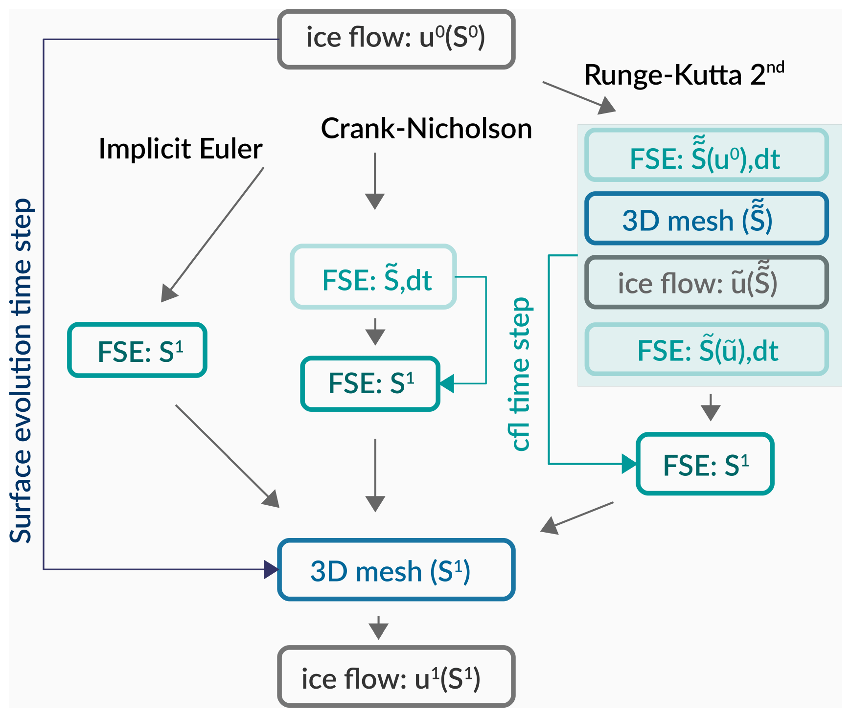
Figure 1 Model chain free-surface evolution schematically drawn for the three different time discretisation schemes: implicit Euler, Crank–Nicholson and Runge–Kutta. Ice flow represents the ice velocity computations, and FSE represents the free-surface evolution. S⁰ denotes the surface elevation at the previous time step, and u⁰ denotes the corresponding velocity field, whereas S¹ is the resulting surface elevation.

5 Simulation framework tests

Firstly, we provide a set of tests that we refer to as “benchmark tests”. These evaluate the simulation framework performance with demanding problems addressing the robustness of our numerical implementation. For these tests, known solutions exist that allow us to perform a quantitative error assessment of the simulation framework. Secondly, we demonstrate the simulation framework capabilities for a glacier case by simulating the free-surface evolution of an alpine valley glacier for different mass balance conditions, assuming no sliding at the glacier bed. In addition, we provide a third glacier case, where we introduce extremely strong gradients through randomly generated input fields of velocity and mass balance rate. All of the tests in this Section are performed with a Crank–Nicholson time discretisation and the time step is derived with the CFL condition using respective maximum values of velocity and mass balance rate and a Courant number of 0.1. In the benchmark tests the artificial ice layer thickness is set to 0.5 m and in the glacier tests it is set to 1 m.

5.1 Benchmark tests

The simulation framework performance is evaluated in terms of its capability to reproduce exact solutions, conserve mass, be numerically stable and converge as a function of spatial resolution. The tests are not performed for geometries in line with glaciological scales but are appropriate to test the performance of the simulation framework.

Regions of steep gradients are most demanding for the simulation framework to produce accurate and numerically stable solutions. Thus, we choose a pyramid-shaped geometry to test its performance. Our initial 3D geometry of the free-surface problem is formed by a flat plane (10×10 m²) and an irregularly shaped pyramid on top of 1 m height, as shown in Fig. 2.

Two different velocity fields and mass balance rate representations are used to test the simulation framework capabilities for a wide range of settings. In the pyramid translation test  the prescribed velocity field introduces a translation (indicated by a blue arrow in Fig. 2) of the pyramid including a vertical displacement due to the effect of a prescribed vertical velocity and mass balance rate field. In the swirling flow test, the pyramid undergoes a forward and reversed swirling flow rotation (indicated by a green arrow in Fig. 2), following the test described in LeVeque (1996).

In this manner, we test the simulation framework by introducing 3D displacement, including overall negative mass changes over time, as well as complex, spatially and temporally variable velocity fields that induce strong distortion of surface geometry.

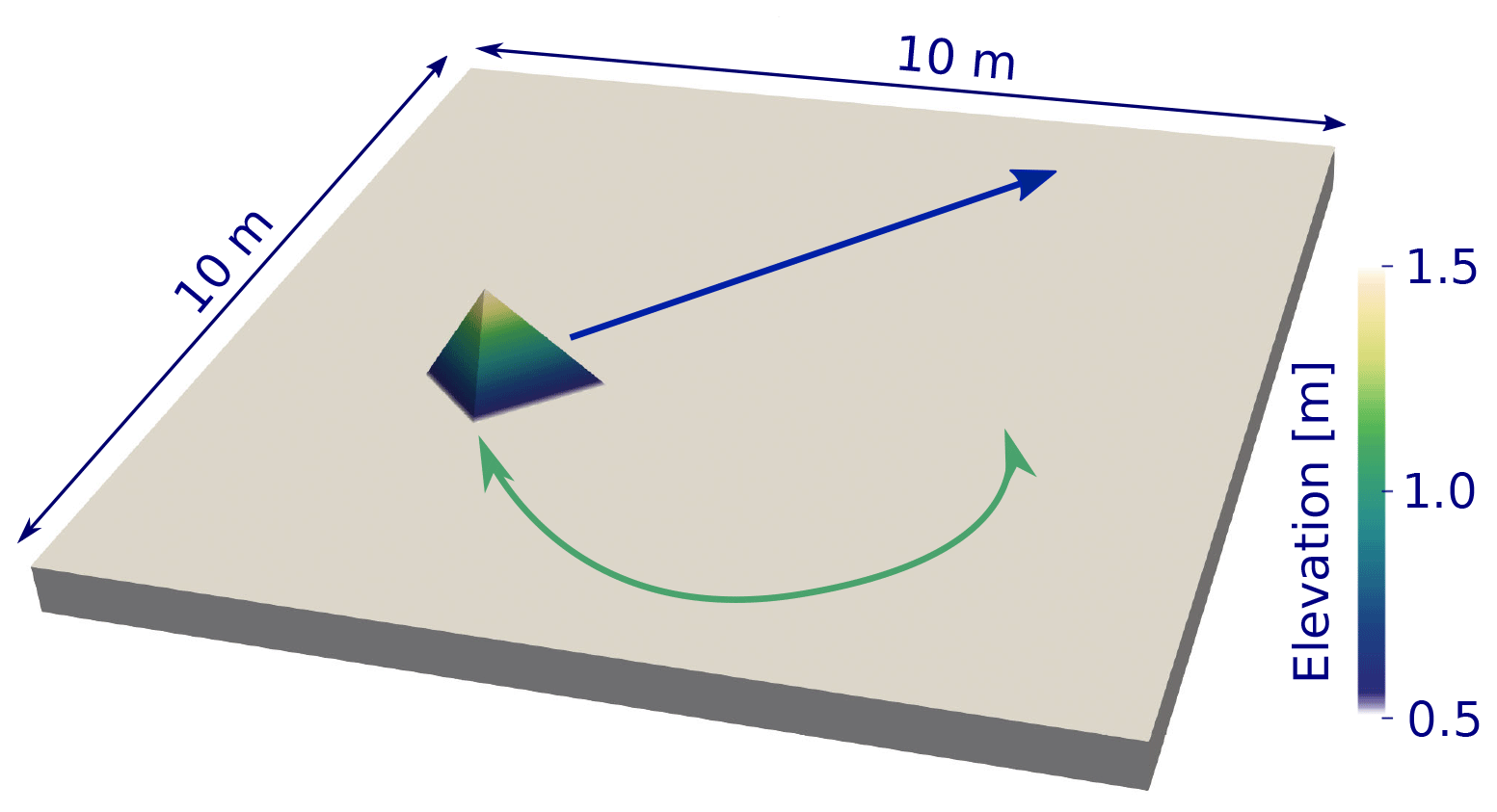
Figure 2 Initial 3D geometry for benchmark tests with surface elevation in colour and arrows indicating the direction of movement for the pyramid translation test in blue and for the swirling flow test in green.

5.1.1 Pyramid translation test

A translational movement is prescribed by a velocity field of u_x=0.85 m s⁻¹ in the x direction, u_y=0.55 m s⁻¹ in the y direction and u_z=0.15 m s⁻¹ in the z direction, whereas the mass balance rate is given by $\dot{a}=-\mathrm{0.30}$ m s⁻¹. This creates a horizontal movement of the test pyramid with an effective vertical downward motion, thus the pyramid's volume will decrease over time. The computations are performed on structured meshes for four different mesh resolutions of $N=\mathrm{125},\mathrm{250},\mathrm{500},\mathrm{1000}$, corresponding to $\text{d}x=\text{d}y=\mathrm{0.08},\mathrm{0.04},\mathrm{0.02},\mathrm{0.01}$ m. For the free-surface computations, a Dirichlet boundary is set so that S=S⁰ on the entire domain boundary, and the time step is derived using the CFL condition and a Courant number of c_max=0.1. A new mesh geometry is created every 0.5 s and simulations evolve until 6.5 s, when the pyramid has almost vanished from the computational domain.

The initial geometry displayed in Fig. 2 has a volume of $V^{\mathrm{0}}=\mathrm{0.37}\dot{\mathrm{6}}$ m³. An exact solution of the volume change for the pyramid over time can be derived using the following set of equations. Starting with the initial pyramid base area A⁰=1.13 m², its temporal change for time t is described as

$$\begin{array}{}\text{(13)}& A_{\text{base}}\left(t\right)=A^{\mathrm{0}}{\left({\displaystyle \frac{h+z\left(t\right)}{h}}\right)}^{\mathrm{2}},\end{array}$$

with h=1 m the initial pyramid height and $z\left(t\right)=(u_z+\dot{a})t$ the effective vertical displacement over time. In our advection case, the horizontal velocities do not have any influence on the pyramid volume. Having derived the changing base area (Eq. 13), we can simply calculate the changing pyramid volume V such that

$$\begin{array}{}\text{(14)}& V\left(t\right)={\displaystyle \frac{\mathrm{1}}{\mathrm{3}}}{A}_{\text{base}}\left(t\right)\left(h+z\left(t\right)\right).\end{array}$$

This exact solution for the pyramid translation test will be used in Sect. 6.1.1 to evaluate the simulation framework performance for different mesh sizes and to demonstrate convergence.

5.1.2 Swirling flow test

For this test, a time-dependent velocity field is prescribed. It induces a swirling flow following the velocity field of Example 9.5 in LeVeque (1996). In the original test, three features of different shapes are advected. Here we apply an identical velocity field but using the pyramid geometry shown in Fig. 2. Due to the prescribed surface velocity, the shape of the pyramid is altered drastically during the test, however the shape will be recovered due to the reverse flow field at the end of the simulation. Comparing initial and final geometry forms a measure of numerical performance, where ideally no differences are detected. This test setup was initially designed for an advection problem. It is also a suitable test in our case, as we describe the free-surface evolution as an advection problem. This test is performed on a mesh with resolution of N=1000, corresponding to $\text{d}x=\text{d}y=\mathrm{0.01}$ m. The time step used to solve the free-surface evolution problem is set to 0.000707 s, which corresponds to a Courant number of c_max=0.1 and a fixed value for the velocity of 10 m s⁻¹. A Dirichlet boundary is set so that S=S⁰ on the entire domain boundary. As a vertical velocity component is missing and a zero mass balance rate is prescribed, total mass has to remain constant in this test.

5.2 Real-world glacier tests

To show the capabilities of the simulation framework for a real-world setting, the temporal evolution of a glacier geometry based on measurements of South Glacier in southwestern Yukon, Canada (60^∘49^′34^′′N, 139^∘07^′34^′′W) is simulated. This valley glacier has an area of 5.3 km² and spans an altitudinal range from 1970 to 2960 m (Flowers et al., 2016).

In order to derive an initial glacier geometry, we use datasets provided in the supplementary information of Farinotti et al. (2017), which are based on Wilson et al. (2013) for the surface elevation and the simulation results of Maussion et al. (2019) for the bed geometry. These datasets have a spatial resolution of 20 m. The computational domain spans a horizontal area of 4.96×6.0 km, covering the glacier area and its surroundings.

For numerous real-world applications, some kind of preprocessing such as smoothing will be applied to DEM data derived from lidar or remote sensing measurements. This serves to reduce noise and related potential unrealistic steep surface features and/or to represent only the level of detail that is required for the problem at hand. For this purpose, we smooth the surface elevation data with a Gaussian filter and a standard deviation (σ) of 2 pixels equivalent to 40 m. A surface topography is created with this smoothed field interpolated to 2 m spatial resolution using bilinear interpolation. An ice thickness field is computed as the difference between the coarse surface (S) and bed (B) elevations and the same smoothing and interpolation procedure is applied before subtracting from the final surface elevation field (S) to provide a bed topography (B). All DEM data processing has been performed with GRASS GIS (GRASS Development Team, 2018).

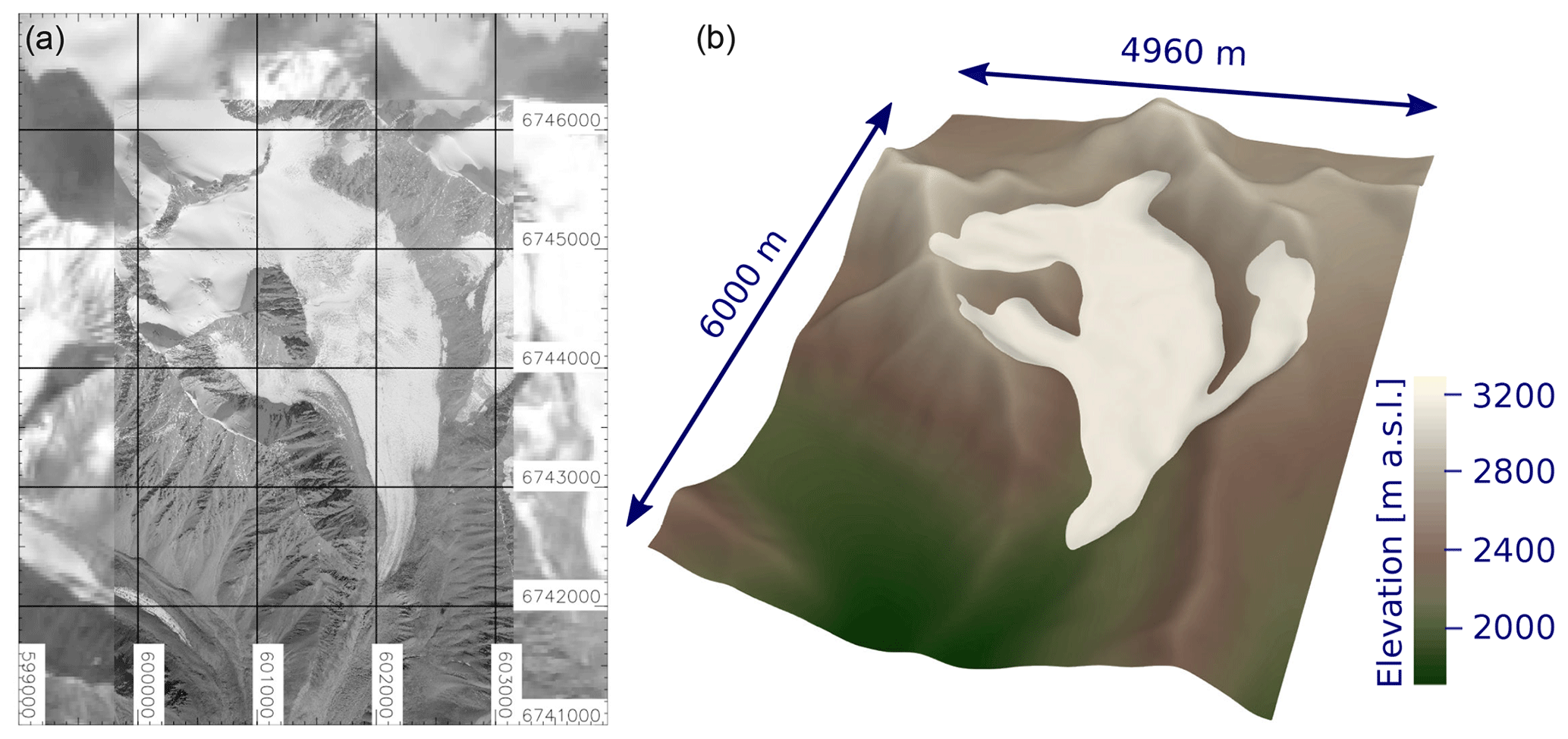
Figure 3 (a) A satellite image (2009) of South Glacier in southwestern Yukon, Canada, a high-resolution image from Schoof et al. (2014), and background filled with Sentinel-2 (ESA) imagery (2018) courtesy of the U.S. Geological Survey. The coordinates are given in UTM zone 7 north. (b) Initial surface elevation of the computational domain. Both panels show exactly the same horizontal extent.

A satellite image of South Glacier and the surface elevation of the smoothed 3D glacier geometry is shown in Fig. 3. In all figures related to the real-world glacier test cases, the top view panels show the same horizontal extent as shown in Fig. 3.

The mass balance rate representations we apply are chosen to best test the simulation framework performance under realistic conditions. However, the computed test results are by no means glacier evolution predictions under current or projected climatic conditions and only serve the purpose to demonstrate simulation framework capabilities. Two different tests are performed using (a) a zero surface mass balance rate and (b) a synthetic elevation-dependent surface mass balance rate. For the velocity computations, the normal velocity component is set to zero at the boundaries so that the domain boundaries act as walls for ice flow. In case of the free-surface computations, natural (Neumann) boundary conditions are applied. The simulations are performed on unstructured 3D and 2D meshes of approximately 40 m (zero mass balance test and elevation-dependent mass balance test) and 20 m spatial resolution (random input fields test). The test setups are provided in the simulation framework repository; see the Code availability section.

5.2.1 Zero mass balance test

The free-surface of the glacier evolves purely due to ice flow. For this purpose, the mass balance rate $\dot{a}$ is set to zero, so no mass is added or removed from the system. The surface evolution time step is set to 2 years, hence new ice velocities are computed every 2 years.

5.2.2 Elevation-dependent mass balance test

The aim of this test is to show the effect of a spatially distributed, time-evolving mass balance rate. For this purpose, we derive a simple mass balance rate from the mass balance dataset provided in the supplementary information of Farinotti et al. (2017) based on Wheler et al. (2014). This mass balance rate is expressed by two piecewise linear functions representing the accumulation and ablation rate purely as a function of elevation separated at an elevation of 2570 $\mathrm{m}\mathrm{a}.\mathrm{s}.\mathrm{l}.$ The mass balance rate is applied over the whole domain, causing strong accumulation in the surrounding initially non-glaciated slopes. This is not quite realistic, as snow redistribution processes (e.g. avalanches and wind drift) are not simulated in our approach, but appropriate to test the simulation framework capabilities. The resulting mass balance rate field is updated according to changes in surface elevation within each time step, whereas a new velocity field is computed every year.

5.3 Random input fields test

In this test, the same initial mesh geometry is chosen as in Sect. 5.2.1, but randomly generated input fields for ice velocity and mass balance rate are used that show unnaturally strong, spatially and temporarily varying gradients. In this manner, the simulation framework is subjected to an extremely demanding problem in order to demonstrate its robustness in terms of numerical stability, as the randomly generated input fields also introduce extremely strong gradients in Eq. (7). To generate the input fields, the maximum velocity of each component for the initial glacier geometry is computed, which are (a) 5.1 m a⁻¹ in the x direction, (b) −6.2 m a⁻¹ in the y direction and −2.2 m a⁻¹ in z direction. From these maximum values, a random noise is subtracted that varies within 100 % of the maximum velocity. The mass balance rate is chosen to be significantly negative and set to −8 m a⁻¹ and a random noise is subtracted that varies within 200 % of this value. A negative mass balance rate causes a decrease of surface elevation and thereby potential contact with the bed constraint. Hence, a negative mass balance regime provides a more stringent test for the simulation framework. The mass balance rate is updated within every time step, whereas velocities are updated every 0.25 years. The frequent update is necessary in terms of stability, as e.g. there is a strong change in surface elevation due to high values of mass balance rate.

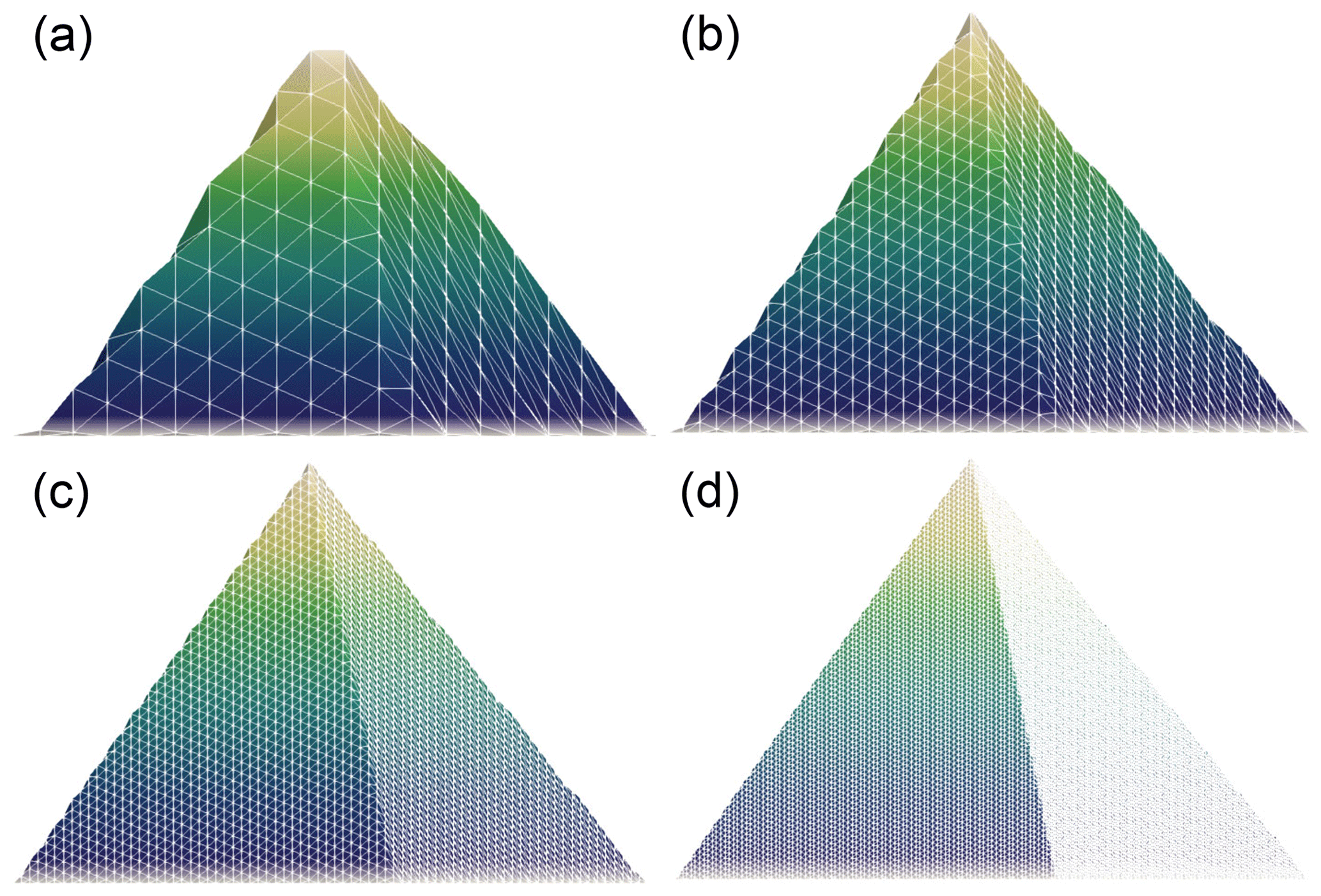
Figure 4 Initial pyramid geometry from left to right for mesh resolutions $N=\mathrm{125},\mathrm{250},\mathrm{500},\mathrm{1000}$ to visualise the quality of feature representation on these meshes.

6 Results

6.1 Benchmark tests

6.1.1 Pyramid translation test

Figure 4 displays the initial geometry represented on all four different mesh resolutions $N=\mathrm{125},\mathrm{250},\mathrm{500},\mathrm{1000}$ (corresponding to $\text{d}x=\text{d}y=\mathrm{0.08},\mathrm{0.04},\mathrm{0.02},\mathrm{0.01}$ m) used in this benchmark. Even though they all try to represent the exact initial pyramid volume of $V^{\mathrm{0}}=\mathrm{0.37}\dot{\mathrm{6}}$ m³, minimal relative initial errors of $\mathrm{1.9}\times {\mathrm{10}}^{-\mathrm{4}}$, $-\mathrm{1.6}\times {\mathrm{10}}^{-\mathrm{5}}$, $\mathrm{5.0}\times {\mathrm{10}}^{-\mathrm{6}}$, $\mathrm{1.37}\times {\mathrm{10}}^{-\mathrm{6}}$ m³ remain.

We evaluate the simulation framework capability to simulate the pyramid translation test for all four different mesh resolutions by comparing numerical results with an existing exact volume change solution (Eq. 14). In Fig. 5a, the volume evolution according to the exact solution (black line) is displayed alongside the four numerical results (coloured lines). Overall, a very good agreement with the exact solution is observed. To produce such an agreement is numerically quite a challenging task, as the variational inequality problem (Eqs. 1 and 2) has to be solved correctly over and over again to recreate the exact solution volume decrease. To highlight the subtle differences that remain, Fig. 5b, displays the absolute difference between the exact and the respective numerical solutions. As mesh resolution increases, the differences decrease and thus the simulation framework converges towards the exact solution.

Testing for shape preservation of the pyramid as it gets advected in the prescribed velocity field is carried out in detail in the benchmark swirling flow test below. Nevertheless, we compare the pyramid's shape at t=4.5 s in Fig. 6, which also displays the pyramid at times $t=\mathrm{0},\mathrm{1.5},\mathrm{3.0},\mathrm{4.5}$ and 6.0 s for the mesh resolution N=1000. The sides of the pyramid are very well preserved, which is a quality indication for the advection implementation. However, the apex point is not equally well preserved and a smoothing of the pyramid top can be clearly seen in Fig. 6b. This smoothing is caused by the continuous function space in which we represent surface elevation and probably some unavoidable numerical diffusion.

Figure 5 (a) Comparison of the exact pyramid volume decrease (black line, Eq. 14) with simulation results (coloured lines) for mesh resolutions $N=\mathrm{125},\mathrm{250},\mathrm{500},\mathrm{1000}$. The term “rsls” indicates the usage of reduced-space methods to solve the variational inequality. Panel (b) shows the absolute difference between the exact solution and simulation results to demonstrate convergence as the mesh resolution increases.

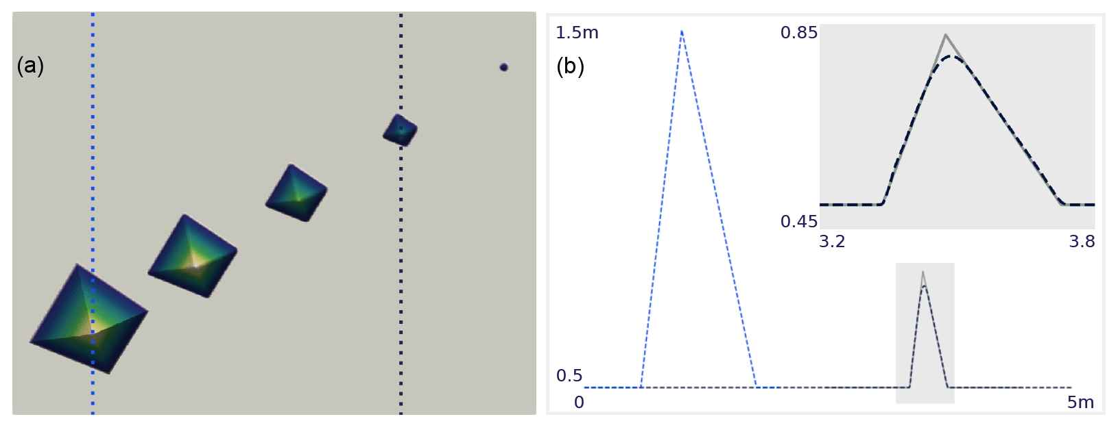
Figure 6 Pyramid translation test. Panel (a) shows the top view of the simulation results for N=1000 at times $t=\mathrm{0},\mathrm{1.5},\mathrm{3.0},\mathrm{4.5},\mathrm{6.0}$ s. Dashed vertical lines indicate the location of the respective profiles in (b) with the dashed light blue line displaying the profile at time 0 s. In (b), simulation results are shown by the dashed dark blue line and compared to the analytical solution (grey line) at time t=4.5 s. The inset on the right shows a zoom of the grey rectangle on the main panel.

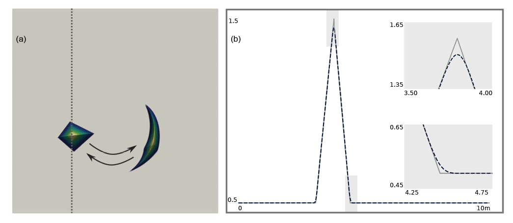
Figure 7 Swirling flow test. Panel (a) shows the top view of simulation results for the 10 m × 10 m domain at time steps 0 and 0.75 s. The dashed vertical line indicates the location of the respective profiles of the simulation results (dashed blue line) and the analytical solution (grey line) at the final time step of 1.5 s shown in (b). The two small inserts show zooms of the grey rectangles on the main panel.

Computations of this benchmark test with reduced-space or semi-smooth methods for mesh resolutions $N=\mathrm{125},\mathrm{250}$ have produced equally good results (not shown here); however, we find the semi-smooth based solver to converge slower and be less stable. Thus we recommend reduced-space methods for our application.

Overall, the benchmark pyramid translation test demonstrates clear convergence and strict volume (i.e. mass) conservation for our simulation framework. Both are paramount simulation framework properties that demonstrate an adequate numerical implementation and thus the applicability of the simulation framework for studying free-surface evolution problems.

6.1.2 Swirling flow test

The results of the swirling flow test are shown in Fig. 7. The simulation framework is capable of reproducing the deformed shape of the pyramid in every point in time and to recover the edges of the pyramid at the end of the simulation. In Fig. 7a, a top view of the results at the start and after half of the simulation duration are shown. The arrows indicate the direction of movement throughout the simulation. In Fig. 7b, the reference shape of the pyramid and numerical solution are compared. In comparison to the reference shape, the pyramid's apex and edges become smoothed, as shown in the inserts, due to the same intrinsic FEM properties as described in the pyramid translation test above. Mass is conserved up to 99.5 %; however, this performance metric of course strongly depends on the mesh resolution.

6.2 Real-world glacier tests

6.2.1 Zero mass balance test

In Fig. 8, the evolution of the glacier surface for a period of 100 years is shown. A decrease in surface elevation in the upper glacier area and its increase in the lower reaches can be observed, which illustrates the expected mass transport. Due to the prescribed mass balance rate of 0 m a⁻¹, the expected total mass change is zero. Throughout the entire simulation of 100 years, the maximum mass change per time step is 0.00032 % of the total ice mass. The total ice mass at the end of the simulation is 99.988 % of the initial ice mass.

Figure 8 Zero mass balance test. View of the difference between initial surface elevation and simulation results at time steps (a) 50 and (b) 100 years and corresponding profiles with shaded surface topography in brown in (c) and (d).

6.2.2 Elevation-dependent mass balance test

In this test, an elevation-dependent mass balance rate is included. The simulation results for a period of 100 years are shown in Fig. 9. There are regions of mass gain and mass loss within the computational domain. Below an elevation of 2570 m, the mass balance rate is negative, hence the lower glacier experiences significant melt and decreases in length and height. At elevations greater than 2570 m, accumulation occurs, causing an increase of surface elevation, which also takes place beyond the initial glacier margin.

With increasing ice thickness, these newly formed ice masses start to move downslope and develop advancing glacier fronts. If these fronts advance into ice-free terrain, at some point the strict solver convergence criteria might not be met anymore when using the Crank–Nicholson time discretisation (see Sect. 7 for details on this problem). In the course of this simulation, this happens only for one single time step at 86 years. However, if the total variation diminishing Runge–Kutta scheme (with an additional SOLD stabilisation term) is used after a time step of 80 years, solver convergence is also guaranteed for this situation.

Figure 9 Elevation-dependent mass balance test. View of the difference between the initial surface elevation and simulation results at time steps (a) 50 and (b) 100 years and corresponding profiles with shaded surface topography in brown in (c) and (d).

6.3 Random input fields test

In this test, the negative mass balance rate removes the glacier completely after a total of 11.25 years, which is simulated with 225 time steps. In Fig. 10, the initial surface elevation and the evolution of the free-surface for two distinct time steps (2.5 and 6.75 years), as well as the corresponding profiles are shown. Due to the strong spatial variations in the prescribed velocity and mass balance fields, the glacier surface becomes heavily undulated. The simulation framework is capable of reproducing this behaviour without introducing any numerical instabilities and thus demonstrates its capability to handle highly complex and variable input fields.

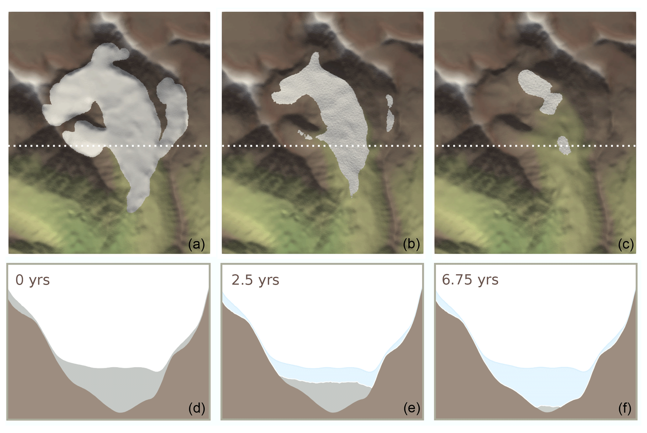
Figure 10 Random input fields test. The view of the surface elevation that exceeds the bed constraint in white and bed constraint in colour at (a) the start of the simulation, at (b) 2.5 and (c) 6.75 years. Corresponding profiles of surface elevation (silver), bed constraint (brown) and initial surface elevation (light blue) in (d)–(f). The elevation on the y axis is shown on a 4 : 1 scale and is thus quite exaggerated.

7 Stability issues of finite-element methods for scalar, convection-dominated equations

When solving the transport problem given in Eqs. (2) and (1), we have to rely on numerical methods to describe complex glaciological problems (as presented in Sect. 5.2) that have arbitrary initial values and arbitrary source functions (Bueler et al., 2007). We require these numerical approximations to be mass conserving and restricted to an admissible interval as prescribed by the local constraints (e.g. bedrock elevation). Equation (2) can be seen as an advection–diffusion equation in the hyperbolic limit, where advection is predominant, and hence it falls into the category of advection-dominated advection–diffusion problems. It is a known problem that for this kind of partial differential equation, standard continuous Galerkin FEMs can lead to the development of unphysical spurious oscillations (e.g. John et al., 2018b). These occur at sharp layers, which is a term referring to locations where strong gradients in the solution are present. The width of sharp layers is typically much smaller than the mesh size and hence cannot be resolved by these methods (John et al., 2018b).

For this reason, from the outset we included the SUPG stabilisation approach (see Sect. 3). Previous studies have shown that this method efficiently inhibits the development of spurious oscillations by introducing numerical diffusion in streamline direction (e.g. Bochev et al., 2004). The SUPG stabilisation technique proved to be effective for many of our glacier tests as well, given the solution is sufficiently smooth.

However, in performing tests for a diverse set of mass balance conditions, occasionally for very steep advancing glacier fronts, unphysical spurious oscillations developed; i.e. the solution is non-smooth for the respective mesh size. Motivated by this observation, we developed an idealised hill test to study these stability issues in detail and analyse the performance of different stabilisation schemes for this application. The idealised hill test is explicitly designed to test the robustness of the simulation framework under the most demanding conditions. To study the problem in detail we distinguish between two cases, steep glacier fronts advance into (i) an already ice-covered domain or (ii) initially ice-free terrain, and hence the bed constraint is potentially affected. In this test, a prescribed elevation-dependent mass balance rate leads to ice accumulation on a Gaussian-shaped hill (see Fig. 11a) that is initially ice-free (configuration ii) or on the same geometry but with an initial ice layer of 10 m thickness covering the entire domain (configuration i). The mesh of the initial geometry is shown in Fig. 11a. For both cases, the mass balance rate is prescribed to increase linearly from for case (i) 0–6 m a⁻¹ (at 9–100 $\mathrm{m}\mathrm{a}.\mathrm{s}.\mathrm{l}.$) and for case (ii) from 0 to 5 m a⁻¹ (at 0–100 $\mathrm{m}\mathrm{a}.\mathrm{s}.\mathrm{l}.$). This leads to accumulation of large amounts of ice in a yearly interval causing the build-up of ice, which is transported downslope in a wave. The resulting ice flow causes the ice front to steepen when it reaches the foot of the hill, hence posing a severe test for the simulation framework. The test runs for 30 years with a yearly velocity update.

The resulting surface elevation after 24 years using the SUPG stabilisation technique and Crank–Nicholson time discretisation is shown in Fig. 11b and a cross-profile of surface and bed elevation is shown in Fig. 11c for configuration (ii). The corresponding results for configuration (i) are shown in Fig. 12 but for 23 years of simulation. We chose to show the resulting surface elevation for the simulation time step where oscillations are most prominent, in order to best discuss their characteristics. The spurious oscillations in the solution are clearly visible; however, they remain stable for both cases, i.e. they do not increase significantly over simulated time. When ice flows into a previously ice-free region, spurious oscillations develop but the negative part of the oscillations most likely becomes efficiently suppressed by the constrained solver. However, if large enough spurious oscillations develop, this eventually can lead to non-convergence of the constrained solver due to the interference with the bed constraint. When the domain is entirely ice-covered, both positive and negative oscillations can arise, but as the bed constraint is not affected, solver convergence is still achieved even if oscillations develop.

Figure 11 In (a) the ice-free geometry mesh formed by a Gaussian-shaped hill in flat terrain and in (b) the simulated surface elevation after 24 years (standard continuous Galerkin stabilised with SUPG) is shown with a cross-profile of surface (blue) and bed (grey) elevation in (c).

7.1 Solution strategies

We have implemented a diverse set of different stabilisation techniques in order to find a model setup that is capable of simulating the advance of steep glacier fronts in a numerically stable manner; in particular, we aim for simulations that reproduce steep fronts but without spurious oscillations and meeting stringent convergence criteria.

Firstly, in addition to the SUPG method, we tested the following spatial stabilisation approaches: (1) continuous interior penalty (CIP, Burman and Hansbo, 2004), (2) spurious oscillations at layer diminishing (SOLD, John and Knobloch, 2008), (3) fourth-order bubble-enriched functions (BR, e.g. Brezzi et al., 1992) and (4) discontinuous Galerkin with upwinding (DG). No separate implementation for the Galerkin least-squares stabilisation method (GLS) can be given, as GLS becomes equivalent to the SUPG method (e.g. Donea and Huerta, 2003) for hyperbolic equations as in our case. All of these stabilisation approaches either add a new term to the variational form of Eq. (2) and/or use a different type of function space. Hence, they can readily be implemented in the model code thanks to the versatility of the FEniCS software. Details of the implementation of individual methods can be found in Sect. 2 and the open-source model code accompanying this paper. There is another class of spatial stabilisation techniques, flux-corrected transport schemes, which showed promising performance in previous studies. However, more analyses for the application in cases of anisotropic meshes and non-linear problems are required (e.g. Barrenechea et al., 2018). We did not include a representative method for this class, as these operate directly on the algebraic level, and thus implementation is not as straightforward as for those schemes that modify the variational form of Eq. (2).

Secondly, we introduce adaptive mesh refinement (AMR) in order to increase local mesh size in the vicinity of sharp layers, but without drastically increasing computational costs, which would be the case for mesh refinement of the entire domain. The SUPG method is supposed to work more efficiently with increasing mesh size and hence increasing capability to resolve sharp layers. The adaptive mesh refinement scheme is based on local surface slope and ice thickness. If the surface slope and ice thickness at any point exceed a threshold, an attractor field is introduced in the gmsh file, whereby refinement of the specified region is facilitated. The mesh refinement is performed once per surface evolution time step (likewise for the 3D and 2D mesh).

Thirdly, in addition to the semi-implicit Crank–Nicholson time discretisation, we test the backward Euler (BE) and the second-order Runge–Kutta (RK2) method. For the RK2 method, we combine the SUPG and a SOLD method in terms of spatial stabilisation, similar to Brinkerhoff and Johnson (2013). The RK2 time discretisation increases stability due to the total variation diminishing property, as well as by increasing the coupling of free-surface evolution and velocity computations.

Finally, we use a structured mesh (ST) and the SUPG stabilisation approach in order to test the influence of mesh anisotropy.

7.2 Simulation results

Simulation results for configuration (i) are shown in Figs. 12 and 13. Regarding the different spatial stabilisation techniques for configuration (i), all of them produce stabilised solutions, meeting the required solver convergence criteria. However the results show spurious oscillations of varying magnitude, except for the CIP method. As solver convergence is guaranteed and the oscillations remain stabilised, this is a manageable problem.

However, if ice flows into an ice-free region (configuration (ii); see Figs. 11 and 14), results of the SUPG and BE approaches display oscillations and do not guarantee solver convergence throughout the simulation period of 30 years. Compared to the SUPG results, the backward Euler time discretisation leads to a slightly smoother glacier front, and the magnitude of the oscillations is smaller. The SOLD and BR methods do guarantee solver convergence throughout the entire simulation period; however, the results show spurious oscillations of similar magnitude. Employing the CIP method to stabilise Eq. (2) provides oscillation-free results and stringent solver convergence; however, this comes at the cost of significant artificial smoothing. The amount of smoothing depends on the choice of the stabilisation parameter γ (see Eq. 10). Performing a set of tests with different choices of γ, we determined γ=0.75 to be a reasonable choice for this specific test, as greater values lead to drastic smoothing and smaller values lead to enhanced oscillations. The SUPG method, in combination with adaptive mesh refinement, leads to a decrease of spurious oscillations; they occur at a later stage and solver convergence is guaranteed throughout the simulation period of 30 years. However, as soon as the advancing fronts become close to vertical, the distinctly finer mesh size is also not capable of resolving the extremely sloping surface adequately in a continuous function space.

If the second-order Runge–Kutta time discretisation is used, oscillations become smaller and solver convergence is guaranteed throughout the simulation period of 30 years. However, computational costs are drastically increased, as velocity updates are required for each time step, and those are by far the most computationally expensive tasks. If simulations are performed on structured meshes, spurious oscillations still develop to some degree, but the SUPG method proves to produce numerically stable results regarding solver convergence. The superior performance in cases of structured meshes seems to stem from the fact that the stabilisation parameter τ (see Sect. 3) is mesh size dependent. The major drawback of using regular meshes is that we lose the ability to employ localised mesh refinement and to represent complex topographies in a detailed manner.

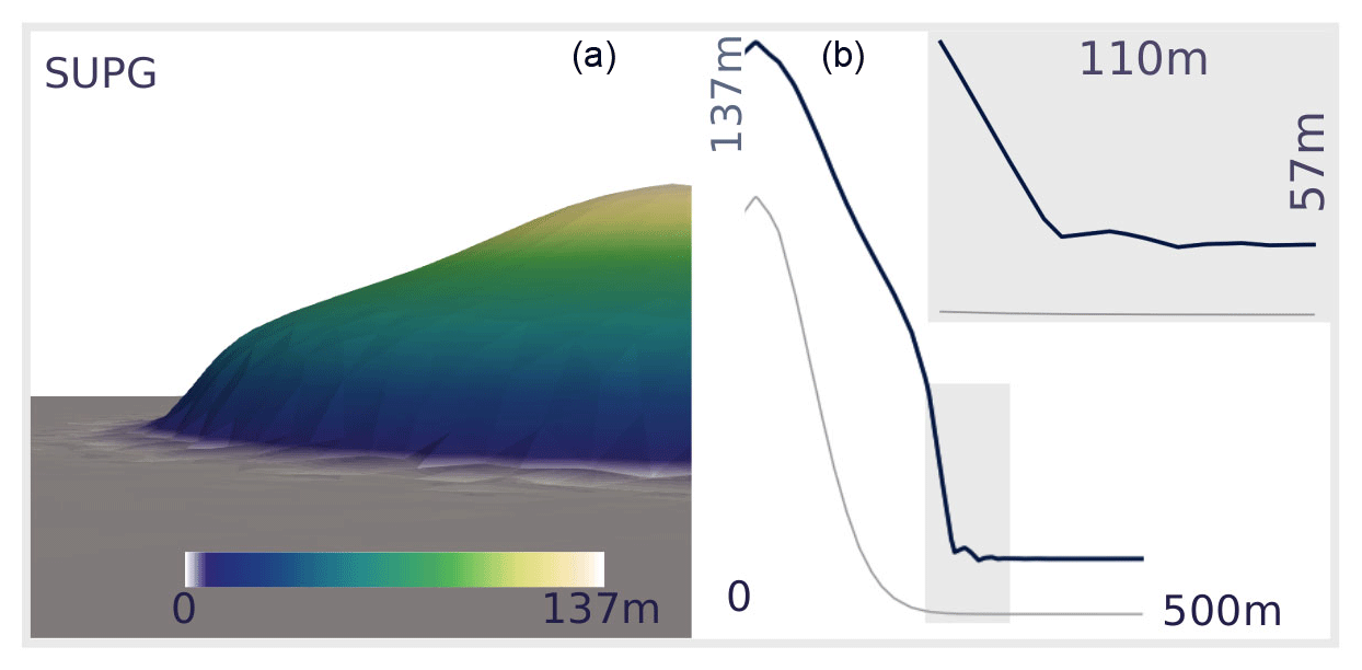
Figure 12 Panel (a) shows the result of the hill test for stabilised simulations after 23 years using the SUPG approach and Crank–Nicholson time discretisation. Panel (b) shows a cross-profile along the y axis of surface (blue) and bed (grey) elevation. The inset shows a zoom of the opaque grey regions.

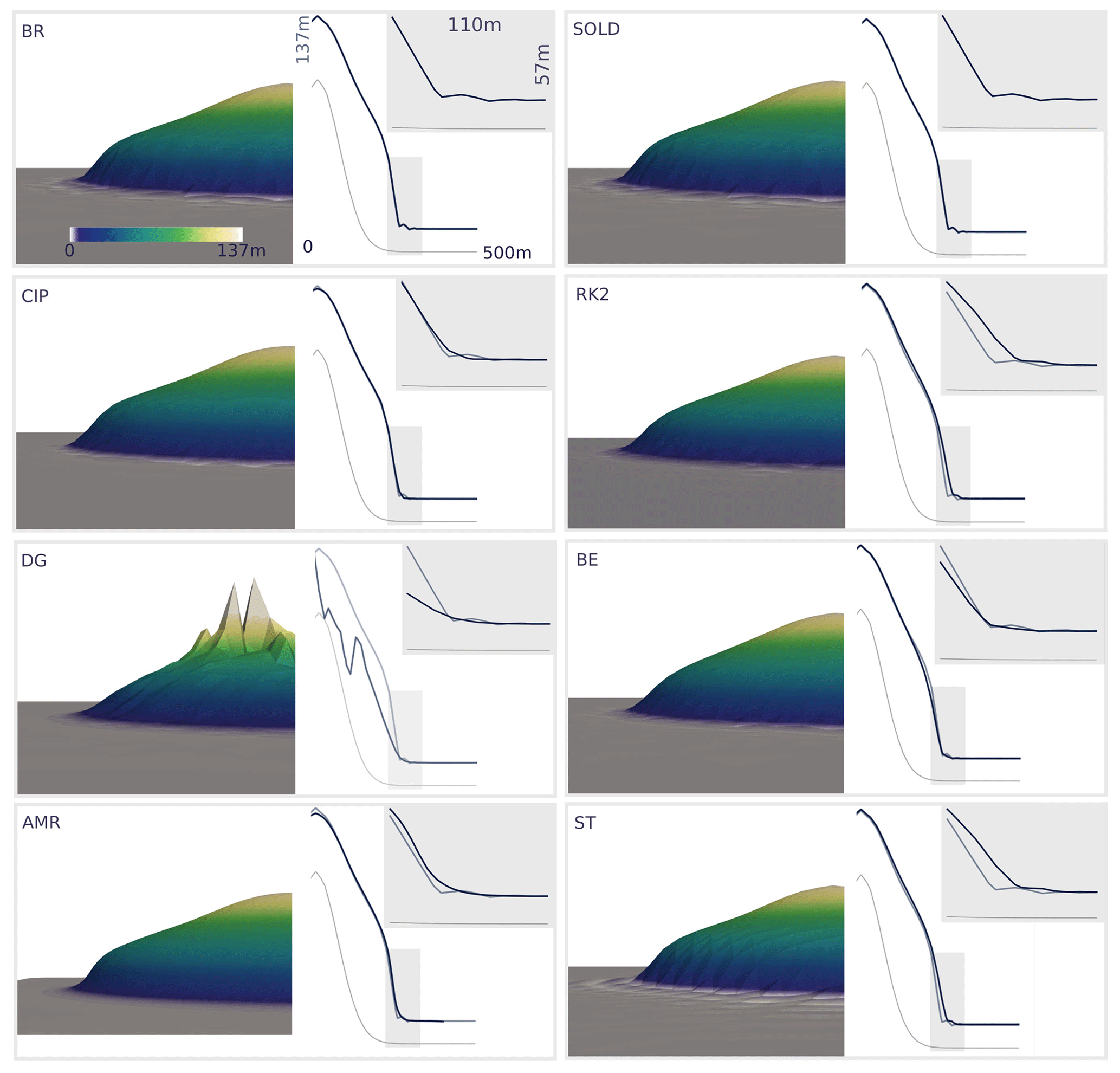
Figure 13 The left panels show results of the hill test for stabilised simulations after 23 years using BR (bubble-enriched), CIP (continuous interior penalty), DG (discontinuous Galerkin), AMR (adaptive mesh refinement), SOLD (oscillations at sharp layer diminishing), RK2 (Runge–Kutta time discretisation), BE (backward Euler time discretisation) and ST (structured mesh). The right panels show a cross-profile along the y axis of surface (blue) and bed (grey) elevation; insets show a zoom of the opaque grey regions; the bold grey line indicates the reference solution using the SUPG and Crank–Nicholson setup (see also Fig. 12).

Figure 14 The left panels show results of the hill test for stabilised simulations after 24 years using BR (bubble-enriched), CIP (continuous interior penalty), DG (discontinuous Galerkin), AMR (adaptive mesh refinement), SOLD (oscillations at sharp layer diminishing), RK2 (Runge–Kutta time discretisation), BE (backward Euler time discretisation) and ST (structured mesh). The right panels show a cross-profile along the y axis of surface (blue) and bed (grey) elevation; insets show a zoom of the opaque grey regions; the bold grey line indicates the reference solution using the SUPG and Crank–Nicholson setup (see also Fig. 11).

7.3 Potential remedies

The presented study suggests that, at the moment, solutions that produce oscillation-free FEM simulations with stringent solver convergence criteria, for the case of steep advancing glacier fronts, based on a time-dependent, non-linear partial differential equation (PDE) solved on an anisotropic mesh, but without introducing significant artificial smoothing or unaffordable mesh sizes, seem to be still somewhat out of reach. A comprehensive study with the elucidating title: “Finite Elements for Scalar Convection-Dominated Equations and Incompressible Flow Problems – a Never Ending Story?” by John et al. (2018b) highlights the remaining problems and open questions in this field.

If the solution is sufficiently smooth, the SUPG method is a valid choice for stabilising the simulations even if the bed constraint is affected. However, if steep advancing fronts develop, further stabilisation is favourable. All tested stabilisation approaches provide stabilised solutions that meet the stringent solver criteria for configuration (i), whereas not all of the presented stabilisation approaches achieve strict solver convergence for configuration (ii) where ice flows into ice-free regions. Stabilised solutions come either at the cost of significant smoothing of sharp layers, drastically increased computational costs or results that are not entirely free of oscillations. For highly detailed studies of glacier geometry change for complex cases, techniques that introduce significant artificial smoothing (e.g. the CIP method or backward Euler time discretisation) are unfavourable because this causes smoothing of steep glacier fronts, for example. However, if smoothing is acceptable for the problem at hand, these approaches can enhance stabilisation and therefore the likelihood of convergence. If smoothing is not desirable, (a) a Runge–Kutta time discretisation (as suggested in Brinkerhoff and Johnson, 2013) and (or in combination with) (b) high spatial resolution through adaptive mesh refinement or (c) the use of structured meshes proved to be most promising in providing high-quality results.

In the case of advancing fronts into ice-free regions, another important remedy is the separation of the domain into subdomains. If the full form of Eq. (7) is solved only where ice is flowing, oscillations cannot develop outside of this domain. If the hill test is performed without the separation into subdomains, spurious oscillations greatly increase in magnitude and spatial extent and cause solver divergence already at an earlier stage. Hence, reasonable definition of subdomains actually serves as another remedy for the development of spurious oscillations and also greatly helps to increase solver convergence.

8 Discussion

From a mathematical perspective, solving this free-boundary problem allows us to provide a physical treatment of a retreating or advancing ice margin. This is not the case in most lower-order ice flow models, which often utilise numerical schemes that include ad hoc treatments for the free ice margin (see Jarosch et al., 2013; Bueler, 2016a, for an overview). Our approach eliminates the need to perform any ad hoc post-processing step dealing with negative ice thickness resulting from regions where the negative mass balance rate per time step is greater than the actual thickness of remaining ice. It has been demonstrated that such post-processing steps often result in mass conservation violations (e.g. Jarosch et al., 2013). As mass conservation is not inherent for FEM methods, we chose to thoroughly check mass conservation for different cases where the actual mass change is known. In the benchmark pyramid translation test, a non-zero mass balance rate is applied, but we can compute the expected mass of the pyramid at any point in time using its reference shape, whereas no mass change is expected for the benchmark swirling flow test and the glacier zero mass balance test. When simulating the evolution of a glacier including a realistic representation of glacier mass balance rate, mass is constantly added or removed from the system. This is a non-trivial problem, implying that overall mass can change within the course of the free-surface evolution computations. Furthermore, expected mass changes cannot be computed directly without any ad hoc procedures, due to the constraint on the surface elevation. To ensure mass conservation for FEM methods, mesh resolution is crucial but it is hard to estimate the required mesh size a priori. Convergence tests can indicate the required mesh size to ensure mass conservation and correct representation of glacier geometry changes due to ice flow and mass balance rate. In this respect, the choice of an appropriate coupling between velocity computations and free-surface evolution (surface evolution time step) regarding the specific conditions of the problem at hand is also vital. Furthermore, one has to keep in mind that the velocity field itself is an approximation as it is solved via FEM on a mesh of finite spatial resolution. Hence, any errors in this quantity could propagate into the free-surface evolution. For example, in a recent study by John et al. (2018a), it has been shown that for a mantle convection model, a coupled system of the stationary incompressible Stokes equations and the convection–diffusion equation, the error of the solution in one problem has an impact on the solution of the other problem.

The simulation framework presented here performs simulations on meshes that also include the surrounding landscape of a glacier. This allows us to represent processes that require knowledge about the surrounding topography, and to simulate glacier advance into previously ice-free terrain. Furthermore, as the computational domain can be divided into different subdomains it is possible to solve individual forms of Eq. (7) for each subdomain all at once. Hence, individual processes can be included for each subdomain, and this can reduce computational costs, for example, if computationally expensive tasks are only solved on relevant parts of the domain. The definition of these subdomains is straightforward and can be updated whenever required, as long as the delineation is based on ice thickness, surface slope, velocity or mass balance rate fields. Other criteria could be implemented if needed. In the presented simulations, the domain is divided according to glacierised and ice-free regions, so that for ice-free regions, the free-surface evolution can be computed solely as a function of the mass balance rate, and potential effects of the artificial ice layer can be excluded. Furthermore, as shown in Sect. 7.3, this is also beneficial in terms of numerical stability.

We have tested the simulation framework capabilities for a diverse set of problems ranging from specific benchmark tests to complex applications for a real-world glacier geometry. The results of the benchmark tests show that the simulation framework is able to reproduce analytical results for challenging geometries (pyramid translation test) and complex flow cases (swirling flow test) and it conserves mass well even in the case of overall mass change (pyramid translation test). However, a thorough stability analysis showed that if very steep, advancing glacier fronts develop, spurious oscillations might arise.

The SUPG approach, as well as the other stabilisation schemes presented in Sect. 7.1, could successfully stabilise the solution but had variable success in suppressing spurious oscillations at sharp layers. In the case of glacier advance into ice-free terrain, these oscillations affect the bed constraint and hence can eventually lead to convergence problems of the constrained solver. We have identified that dividing the entire domain into subdomains and solving the full form of Eq. (7) only in the relevant domains serve as a potential remedy for this problem. If the full form of Eq. (7) is solved in a subdomain defined by the glacierised part including a velocity-dependent buffer zone but not reaching beyond this zone, spurious oscillations can successfully be inhibited by restricting the advection term to these parts of the domain.

In addition to this, the weak coupling between velocity computations and free-surface evolution (as a consequence of linearisation for the Crank–Nicholson and backward Euler schemes; see Sect. 3) is not favourable if steep, advancing glacier fronts develop. In this case, a total variation-diminishing time discretisation, e.g. a Runge–Kutta scheme, performs much better in terms of numerical stability and accurate representation of surface elevation, as has been proposed in Brinkerhoff and Johnson (2013). In the elevation-dependent mass balance test of the glacier tests, the Crank–Nicholson scheme fails in terms of solver convergence when steep glacier fronts advance into ice-free terrain for one time step. Using the Runge–Kutta method and additional SOLD stabilisation provides stable results and also guarantees solver convergence for this situation. This example illustrates that appropriate methods have to be chosen according to the problem at hand; e.g. for complex situations like steep advancing fronts, a tighter coupling between velocity computations and free-surface evolution is favourable. However, using the Runge–Kutta time discretisation comes at the cost of drastically increased computational effort as the number of required 3D velocity computations increases. In the case of smooth solutions, the Crank–Nicholson and backward Euler schemes, i.e. a much weaker coupling of velocity computations and free-surface evolution, proved to be an acceptable compromise between low computational costs and accuracy. Furthermore, the use of structured meshes or adaptive mesh refinement proved to also decrease the magnitude of spurious oscillations and accordingly the likelihood of non-convergence (see Sect. 7.2). This stems from the fact that (i) the SUPG stabilisation parameter is mesh size dependent and structured meshes are favourable and that (ii) the capability to resolve sharp layers increases with increasing spatial resolution, which is the case for adaptive mesh refinement. In cases of non-convergence or if numerical instabilities develop, we suggest checking the time stepping and time discretisation scheme, mesh quality, and mesh size and to revisit the definition of subdomains. In case of coarse meshes, the subdomains can reach far into the artificial ice layer, which is not favourable and facilitates the development of oscillations. This means that for complex geometries, a minimal spatial resolution has to be provided depending on the complexity, e.g. steepness, of the actual topography, which is also crucial in terms of mass conservation.

Simulations usually spend most of the overall computation time (>95 %) at the Stokes problem. Due to the complex mesh modifications and direct operations on the degrees of freedom, the free-surface computations are not parallelised, which is not problematic regarding their share of the overall computational costs.

9 Conclusions

The free-surface evolution of flowing ice formulated as a variational inequality (proposed earlier by, e.g. Jouvet and Bueler, 2012) has been implemented in a new, open-source numerical simulation framework.

This simulation framework automates (1) mesh generation, (2) computation of 3D ice velocity based on a full Stokes approach, (3) simulation of free-surface evolution due to ice flow and mass balance rate, including the glacier surroundings and fully accounting for the constraint of S≥B, and (4) generation of updated 3D geometry meshes.

It offers the option to choose different time discretisations and spatial stabilisation approaches, as well as adaptive mesh refinement. This is of special interest for detailed studies of glacier geometry change or given complex topographical conditions. These features make it a highly versatile tool for different glaciological applications. The simulation framework can also be applied for highly complex cases of multiple glaciers (including their initial formation) within one domain and for a wide range of glacier mass balance conditions. The option for defining individual subdomains makes it straightforward to add processes that are relevant for individual subdomains only.

We have proposed a set of benchmarks (see Sects. 5.1 and 7) to evaluate numerical implementations of free-surface flows as variational inequalities. By performing these tests, numerical stability, mass conservation, shape preservation, and the ability to reproduce realistic glacier states can be assessed. Our simulation framework performs well in those challenging tests and demonstrates mass conservation even in the case of overall strong mass changes (i.e. mass balance) for sufficiently fine meshes. It is important to test these aspects, as simulation results can look realistic but this does not alone ensure correctness of the results. Furthermore, the idealised hill test simulations highlight potential limitations of the presented approach and provide information about which conditions require caution in order to ensure high-quality results. To demonstrate the suitability of our approach for real-world glaciological applications, we have presented several results with glaciological input data and simulation periods of 100 years.

The physically consistent, free-surface simulation capability of our framework presented here is not only suitable for glaciological applications, but for many free-surface flows found in geoscience. Our proposed benchmark tests are highly suitable to evaluate numerical implementations of free-surface flows on a general level. Our review of spatial stabilisation methods and time discretisation approaches will be useful in choosing a suitable combination for a given simulation task, as it is apparent that there is no single suitable approach for all glaciological applications. Therefore we hope that our provided benchmarks find wider use in assessing the numerical performance of existing and upcoming models.

Appendix A: Preprocessing, mesh generation and remeshing

The model setup facilitates the generation and use of unstructured or structured triangular (2D) or tetrahedral (3D) meshes. These are created with gmsh (Geuzaine and Remacle, 2009), an open-source finite-element mesh generator. The standard setup is to employ unstructured meshes, which offers the advantage of potential mesh refinement within regions of interest and the increased ability to represent complex geometry. In case of adaptive mesh refinement we employ gmsh's capabilities to introduce attractor fields to create regions of different mesh size.

The implementation of a versatile meshing algorithm facilitates generation of high-quality 3D meshes and efficient remeshing of new geometries, which is required for the free-surface evolution. In the preprocessing step, a 3D mesh is generated from a digital elevation model (DEM) that covers the glacier or multiple glaciers of interest and their surrounding terrain, including information on the glacier bed geometry. For this purpose, first a rectangular domain is defined covering the area of interest so that potential glacier advances, as well as processes that require information on the surrounding terrain (e.g. gravitational mass additions from surrounding slopes), can be represented correctly. Its corner coordinates are used to create a STL (stereolithograph) ¹ file for a 3D rectangular box covering the domain of interest using gmsh. This box STL file represents the surface mesh of the desired 3D volume mesh, but initially is just a rectangular box surface, covering the area of interest. In the next step, the DEM is used to directly set the vertical coordinates of the surface and bed elevation at the vertices of this box surface STL file. This updated file is then used to mesh a 3D volume mesh using gmsh. The resulting mesh is fully unstructured. As for the velocity computations, a 3D mesh is required even where the ice thickness ($H=S-B$) is zero; in those regions we also assign a minimal thickness h_af, which we refer to as the “artificial ice layer” for ease of understanding. Due to this artificial ice layer the inequality constraint becomes $S\ge \stackrel{\mathrm{̃}}{B},\stackrel{\mathrm{̃}}{B}=B+h_{\text{af}}$.

There is a second option to generate the 3D mesh. Here, instead of STL files, mesh generation is performed using gmsh's msh file format. In this case, the number of vertical layers can be prescribed, and hence the resulting meshes become structured in the vertical. For this approach, for the corner coordinates of the area of interest a box msh file is meshed instead of a box STL file. This box msh file represents a volume mesh, as a rectangular box covering the area of interest. In the next step, the DEM is similarly used to directly set the vertical coordinates of the surface and bed elevation at the vertices of this box msh file. In this case, the vertical coordinate of the nodes within the volume is also set using the surface and bed elevation combined with the vertical number of layers to evenly distribute the nodes in the vertical. This procedure results in a 3D volume mesh that is structured in the vertical.

If a new mesh geometry is required, this initial box surface STL or box msh file can simply be used to generate a new mesh by setting the vertical coordinates using the new surface elevation information, following the procedure described in the previous paragraph. If the STL file is used, it is re-meshed in order to generate a new mesh. In case of the box msh file, this is not required as the vertical coordinates of all nodes are set using the new surface elevation. As horizontal node coordinates remain fixed, and vertical coordinates are set based fully on the new surface elevation, this procedure represents a remeshing process and no mesh distortion is introduced.

In the standard setup, the horizontal locations of nodes are not changed throughout the simulations. If adaptive mesh refinement is used, these locations might change, and as a result topographical features such as ridges could potentially become smoothed if the nodes of highest or lowest locations are not represented in the modified mesh, even where there is no change due to mass balance rate or ice flow. Hence, it is recommended that regions where important topographic features are located are included in the refinement region even if these lie outside of the glacierised domain.

As the free-surface evolution is a problem that is one dimension lower than the ice velocity computation, the computations are performed on a 2D mesh that covers the horizontal extent of the 3D domain. The following procedure offers a flexible setup that works for any given mesh size in an automatised manner to initially derive the surface and bed elevation, ice velocities and mass balance rate on the 2D mesh. This workflow is illustrated in Fig. A1, including the generation of a new mesh geometry with the new surface elevation (step 5).

First, a boundary mesh of the initial 3D geometry (Fig. A1 (1)) is created, and from this submeshes of the surface and bed are generated with marked surface and bed boundaries (Fig. A1 (3)). On these submeshes, which are 2D surfaces but are still oriented in 3D space, a function for the actual surface elevation, i.e. the vertical coordinate of the submesh, is introduced and the 3D ice velocities (see Fig. A1 (2) are interpolated onto the submesh of the surface. The z coordinates of all the submeshes are then set to zero. On these (now flat) meshes, the elevation of the surface and bed, which was the actual vertical coordinate of the submeshes, are still well defined. This step allows us to evaluate the surface elevations with only the horizontal coordinates as input. The functions representing the elevation of surface and bed, as well as the 3D velocity field, are evaluated at the vertices of the 2D mesh (see Fig. A1 (4)). In Eq. (2), the horizontal and vertical velocity component are required as separate inputs, hence these individual components are defined as individual vector and scalar functions (see Fig. A1 (4), labelled with xy and z). In this manner, surface and bed elevation, as well as velocity fields, can be derived on the 2D mesh from any given 3D mesh, independent of mesh size.

Figure A1 How to derive surface and bed elevation and horizontal and vertical velocity components on the 2D mesh: (1) a 3D mesh of the glacier including its surroundings; (2) a 3D velocity field computed with icetools; (3) a boundary mesh of the 3D geometry and submeshes of surface and bed boundary; (4) surface elevation, bed constraint, horizontal, and vertical velocity as functions defined on 2D computational mesh; and (5) an updated STL file used to create new 3D mesh.