the Creative Commons Attribution 4.0 License.
the Creative Commons Attribution 4.0 License.
 | 10 Dec 2020
Development of a three-dimensional variational assimilation system for lidar profile data based on a size-resolved aerosol model in WRF–Chem model v3.9.1 and its application in PM2.5 forecasts across China
Yanfei Liang
Zengliang Zang
Peng Yan
Yiwen Hu
Yan Zhou
Wei You
The authors developed a three-dimensional variational (3-DVAR) aerosol extinction coefficient (AEC) and aerosol mass concentration (AMC) data assimilation (DA) system for aerosol variables in the Weather Research and Forecasting–Chemistry (WRF–Chem) model with the WRF–Chem using the Model for Simulating Aerosol Interactions and Chemistry (MOSAIC) scheme. They establish an AEC observation operator and its corresponding adjoint based on the Interagency Monitoring of Protected Visual Environments (IMPROVE) equation and investigate the use of lidar AEC and surface AMC DA to forecast mass concentration (MC) profiles of PM2.5 (particulate matter with an aerodynamic diameter of less than 2.5 µm) across China. Two sets of data were assimilated: AEC profiles captured by five conventional Mie scattering lidars (positioned in Beijing, Shijiazhuang, Taiyuan, Xuzhou, and Wuhu) and PM2.5 and PM10 MC data obtained from over 1500 ground environmental monitoring stations across China. Three DA experiments (i.e., a PM2.5 (PM10) DA experiment, a lidar AEC DA experiment, and a simultaneous PM2.5 (PM10) and lidar AEC DA experiment) with a 12 h assimilation period and a 24 h forecast period were conducted. The PM2.5 (PM10) DA reduced the root mean square error (RMSE) of the surface PM2.5 MC in the initial field of the model by 38.6 µg m−3 (64.8 %). When lidar AEC data were assimilated, this reduction was 10.5 µg m−3 (17.6 %), and a 38.4 µg m−3 (64.4 %) reduction occurred when the two data sets were assimilated simultaneously, although only five lidars were available within the simulation region (approximately 2.33 million km2 in size). The RMSEs of the forecasted surface PM2.5 MC 24 h after the DA period in the three DA experiments were reduced by 6.1 µg m−3 (11.8 %), 1.5 µg m−3 (2.9 %), and 6.5 µg m−3 (12.6 %), respectively, indicating that the assimilation and hence the optimization of the initial field have a positive effect on the PM2.5 MC forecast performance over a period of 24 h after the DA period.
- Article
(6863 KB) - Full-text XML
- BibTeX
- EndNote


Aerosol data assimilation (DA) generates a three-dimensional (3D) gridded analysis field capable of describing the spatial distribution of aerosols by integrating numerical forecasts produced by an air quality model (AQM) and measured aerosol data. With integrated information from various sources, this analysis field can more accurately describe the 3D distribution pattern of aerosols (Carmichael et al., 2008; Benedetti et al., 2009; Sandu and Chai, 2011; Bannister, 2017). The analysis field generated by DA can be used to effectively study atmospheric aerosol transmission patterns through an analysis of the products of a certain time series and, on this basis, further examine the effects of aerosols on human health, the environment, the weather, and the climate (Baraskar et al., 2016; Haywood and Boucher, 2020). The analysis field can also be used to determine the initial chemical conditions for an AQM. Therefore, improving the accuracy of the initial chemical conditions and enhancing the forecasting performance of the AQM for aerosols (Wu et al., 2015).
Compared to those of meteorological and marine DA, aerosol DA techniques are still undeveloped, and there is a lack of variety when it comes to assimilable measured data, which mainly include conventional surface aerosol mass concentration (AMC) data and satellite-derived aerosol optical depth (AOD) data. Of these two types of data, surface AMC data provide mass concentration (MC) information for near-surface aerosols directly. AOD is a measure of the total extinction effects of aerosols in the vertical atmospheric column, which indirectly provide atmospheric column aerosol concentration information. Assimilating either of these two types of data can significantly improve the accuracy of the aerosol analysis field (Tombette et al., 2009; Niu et al., 2008; Schwartz et al., 2012; Jiang et al., 2013; Li et al., 2013; Saide et al., 2013; Yumimoto et al., 2015, 2016; Tang et al., 2017; Peng et al., 2017; Xia et al., 2019; Wang et al., 2020). However, neither AOD nor surface AMC data are able to provide vertical aerosol profiles. Consequently, while these two types of data are abundant, have relatively high horizontal resolutions, and have excellent coverage, they play a limited role in optimizing the vertical structure of aerosols in the analysis field. To further improve the accuracy of the simulated vertical structure, it is necessary to assimilate data that contain vertical aerosol profile information. Zang et al. (2016) assimilated aircraft-measured vertical concentration profiles of aerosol components and found that while the profile data were limited in quantity and covered a relatively small area, they could still significantly improve the forecast accuracy of an AQM. Since direct observations of concentration profiles are labor-intensive and expensive, relatively few studies involving the acquisition and assimilation of this type of data have been reported.
Aerosol lidar can be used to capture aerosol-backscattered laser signals at various heights. By inverting these signals, the aerosol extinction coefficient (AEC) and aerosol backscattering coefficient (ABC), which indirectly provide vertical AMC profile information, can be determined (Fernald et al., 1984; Sugimoto et al., 2008; Raut et al., 2009). Assimilating these lidar aerosol data can help to improve the accuracy of the vertical structure of aerosols in the analysis field (Tesche et al., 2007; Ganguly et al., 2009; Young and Vaughan, 2009; Burton et al., 2010; Milroy et al., 2011; Sugimoto et al., 2014; Chen et al., 2015). In addition, with the increasing number of lidar stations and the development of lidar network detection technology, studying lidar DA in order to generate more accurate 3D aerosol analysis fields has great potential.
Compared to the assimilation of direct AMC measurements, the assimilation of lidar AEC data faces myriad difficulties, of which establishing an observation operator for the DA cost function is the most challenging. The AEC is the object of the DA (i.e., observation variable), whereas the AMCs of various types of aerosol variables in the AQM must be optimized. To directly determine the optimal model aerosol variables by solving the DA cost function, it is necessary to map the aerosol variables in the AQM to the observation space by conducting a forward process on the observation operator (Kahnert et al., 2008), corresponding to the calculation of the AEC from the AMC. In addition, in three-dimensional variational (3-DVAR) DA, it is also necessary to conduct the adjoint process on the observation operator when calculating the gradient of the cost function (Sandu and Chai, 2011). The computational program for this adjoint process on the observation operator relies on its forward process, leading to a large computational load, and the size of the program code increases nonlinearly with the complexity of the forward process. Moreover, when it comes to aerosol variables, there are many kinds of chemicals and particle-size bins so that the chemical model inherently involves a large computational load. Therefore, when using a variational method to assimilate lidar data, it is necessary to consider both the accuracy and complexity of the observation operator. Currently, there are three main methods that are used to design observation operators:
-
use of the Mie equation directly. Under the assumption that aerosol particles are uniform and spherical, the Mie equation describes the scattering and extinction properties of aerosol particles of any scale with any chemical and physical parameters (Wiscombe, 1980; Cheng et al., 2019). However, because accurately solving the Mie equation involves a nonlinear calculation process that contains iterations, it is extremely complicated to implement, upgrade, and maintain the program for the reverse process on the observation operator. In addition, because of the lack of reliable measurements of essential aerosol parameters (e.g., complex refractive index, particle number spectrum, and hygroscopicity), it is necessary to introduce assumptions about these parameters in DA schemes. This renders it difficult to realize the high-accuracy advantage of DA schemes in practice.
-
use of the Community Radiative Transfer Model (CRTM). This model is advantageous because it gives the Jacobian term needed for the adjoint process on the observation operator when conducting its forward process. Therefore, introducing the CRTM to a DA scheme does not require separate numerical computational programming for the adjoint process on the observation operator (Liu and Weng, 2006). DA schemes based on the CRTM have been applied in AOD DA research and yielded excellent results (Liu et al., 2011). However, the CRTM was developed for the Goddard Chemistry Aerosol Radiation and Transport (GOCART) aerosol scheme in the Weather Research and Forecasting–Chemistry (WRF–Chem) model. As a result, when applying the CRTM to other AQMs and aerosol schemes, it is necessary to design corresponding variable transformation interfaces (Cheng et al., 2019), which introduces additional errors.
-
use of the interagency monitoring of protected visual environments (IMPROVE) equation. The IMPROVE equation maps the relationship between the AMC and the AEC (Lowenthal et al., 2003; Ryan et al., 2005; Pitchford et al., 2007; Gordon et al., 2018). With relatively high computational accuracy, this method has been used to evaluate model performance and the extinction contributions of various aerosols (Kim et al., 2006; Roy et al., 2007; Tao et al., 2009, 2012, 2014; Cao et al., 2012a, b). In addition, as its highest-order term is quadratic, the IMPROVE equation has low nonlinearity. Therefore, using the IMPROVE equation to design an observation operator can significantly reduce the complexity of the DA program. To date, no observation operator design based on the IMPROVE equation and subsequent variational lidar DA have been reported.
Some progress has been made in lidar DA. For example, Sekiyama et al. (2010) used the Kalman filter DA method to assimilate the ABC and AEC profiles acquired by the Cloud-Aerosol Lidar and Infrared Pathfinder Satellite Observations mission and applied the assimilated data to a global chemical transport model. Wang et al. (2013, 2014a, b) studied the assimilation of range-corrected lidar signals using the optimal interpolation DA method and conducted an assimilation experiment based on data captured by 12 lidars positioned in the Mediterranean Basin from the ACTRIS (Aerosols, Clouds, and Trace Gases Research InfraStructure)/EARLINET (European Aerosol Research Lidar Network) and one lidar positioned on the French island Corsica from the framework of the pre-ChArMEx (Chemistry-Aerosol Mediterranean Experiment)/TRAQA (TRAnsport àlongue distance et Qualité de l'Air). They found that DA improved the PM2.5 forecast performance for approximately 36 h. However, in the above-mentioned studies, sequential DA methods were used, and there was no particular need to take into consideration the complexity of the observation operator. Cheng et al. (2019) assimilated lidar AEC profiles using a 3-DVAR DA method with an observation operator based on the CRTM that was designed for a relatively simple GOCART dust aerosol scheme.
This study presents an observation operator and corresponding adjoint module developed for lidar AEC DA based on the IMPROVE equation, which was introduced into the DA system by Li et al. (2013) and Zang et al. (2016) for the Model for Simulating Aerosol Interactions and Chemistry (MOSAIC) aerosol scheme oriented to the WRF–Chem model. By applying the DA system, DA and forecast experiments were conducted to investigate the application of lidar AEC DA in PM2.5 forecasts across China based on data captured by five lidars (located in Beijing, Shijiazhuang, Taiyuan, Xuzhou, and Wuhu, respectively) as well as on PM2.5 and PM10 data collected at approximately 1500 ground environmental monitoring stations across China.
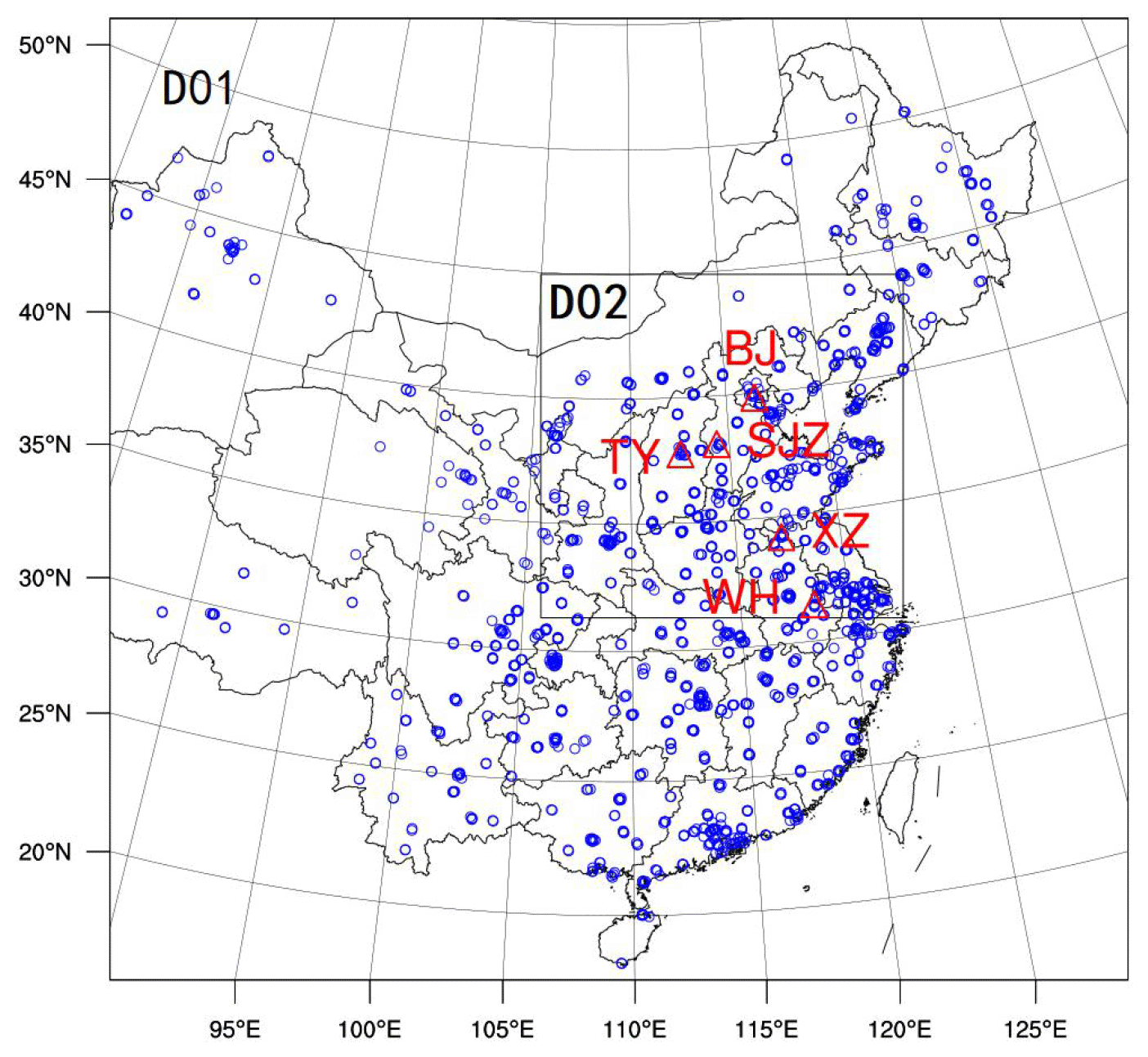
Figure 1The double-nested experimental domain. Red triangles and labeling indicate the locations and names of five lidars, and blue circles indicate the locations of 1500 ground environmental monitoring stations.
2.1 AQM
The WRF–Chem model version 3.9.1 was selected as the AQM. The model has 40 vertical layers between the surface and 50 hPa, with the resolution gradually decreasing from the bottom up. The model domains are double-nested, and the second domain (D02) is centered at 114.57∘ E and 37.98∘ N and has 175×166 grid points with a grid interval of 9 km. D02 covers the central and eastern regions of China (most of North China, northern Central China, northern East China, and eastern Northwest China) (Fig. 1). The MOSAIC_4bin aerosol scheme was adopted for the simulations. This scheme, which will be described in Sect. 2.4, can be used to predict the profiles of eight aerosol types. For each aerosol type, there are four particle-size bins (4bins). The following summarizes the other physical and chemical schemes used in this study: the carbon-bond mechanism version Z (CBMZ) chemical reaction mechanism, the fast-J photolysis calculation scheme, the rapid radiative transfer model for general circulation model (RRTMG) shortwave radiation scheme, the RRTMG longwave radiation scheme, the WRF single-moment 5-class microphysical scheme, the unified Noah land-surface parameterization scheme, the Grell 3D ensemble cumulus parameterization scheme, the Yonsei University planetary boundary layer scheme, and the revised MM5 Monin–Obukhov near-surface layer scheme.
2.2 Data
The AEC profiles used in this study were derived from data captured by five conventional Mie scattering lidars (positioned in Beijing, Shijiazhuang, Taiyuan, Xuzhou, and Wuhu; Fig. 1) at a wavelength of 532 nm between 00:00 and 12:00 Coordinated Universal Time (UTC) on 13 November 2018 (Chen et al., 2019; Zhang et al., 2020). The temporal resolution of the data measured by the lidars in Shijiazhuang, Taiyuan, Xuzhou, and Wuhu was 1 min; that is, data were captured, and a vertical AEC profile was derived every minute. The vertical resolution of these data was 7.5 m; that is, one AEC was determined in one profile 7.5 m away from the next one. The blind zone of these lidars was 100 m; that is, these systems could not effectively capture AEC data between the surface and the height of 100 m. The temporal and vertical resolutions of the AEC profiles captured by the lidar in Beijing were 1 h and 15 m, respectively, and the blind zone of this lidar was 210 m. The relative standard deviation of the aerosol parameter profiles captured by the lidar over Beijing was 20.4 % in the height range of 1–2 km. This lidar was calibrated via comparative observation of several lidars (Chen et al., 2019). The precision of the AEC profiles released by the other four lidars was below the quality margins (25 % of the typical AEC observed in the planetary boundary layer or ±0.01 km−1), as defined by Matthias et al. (2004). However, the relative standard deviation of the aerosol parameter profiles in the height range of 2–5 km released by lidar over Beijing was 35.9 %. To improve the effectiveness of the DA, it was necessary to first perform quality control on and preprocess the original AEC profiles. This ensured that the lidar data matched the numerical model in terms of temporal and spatial resolution. Quality control involved four steps:
-
Entire AEC profiles passing through low clouds and AEC measurements in mid- and high-cloud regions were eliminated. Clouds were defined as regions in which the AEC was higher than m−1 (assuming the AEC in the near-surface layer (below 150 m) was lower than m−1).
-
AEC profile data were subjected to maximum and minimum control. AEC measurements higher than m−1 were each reassigned with a value of m−1. AEC measurements lower than m−1 were eliminated.
-
For spatial continuity, data were required to be continuous within a vertical space Lcon, which was set to be 90 m in this study. Specifically, two metrics were used to examine the spatial continuity of the data. First, the profile with vertical resolution Lres was examined. After the first two steps of quality control, the remaining number of data points (Nremain) within the Lcon could not be less than one-third the total number of data points within the Lcon (). Otherwise, no valid data would be available for the center of the Lcon. Second, the deviation of the valid data from the mean value of the data within the Lcon could not exceed 3 times the standard deviation (SD).
-
Data within the blind zone of a lidar were eliminated. In addition, because lidar signals are relatively weak and AMCs are extremely low above 5000 m, data for the region above 5000 m were also eliminated in this study. After the quality control process, 84.32 % of the original AEC data from the lidar over Beijing were accepted as valid data, and 88.75 %, 54.10 %, 26.74 %, and 10.95 % of the data from the Taiyuan, Wuhu, Shijiazhuang, and Xuzhou lidars, respectively, were valid.
Preprocessing of quality control-treated AEC profiles involved two steps:
-
Temporal and spatial smoothing. Profiles were subjected to moving averaging over 30 m in the vertical direction. Temporally, the AEC profiles were averaged over the previous hour.
-
Data thinning. If there were multiple data points between two adjacent model layers in the vertical direction, only one was selected for assimilation. In this study, the nearest data point below each model layer was selected for assimilation. After processing, the number of assimilated AEC measurements per profile did not exceed 25, as there were no more than 25 model layers between the top of the lidar blind zone and the height of 5000 m.
PM2.5 and PM10 data (hereinafter referred to as PM data) used in this study, including 1 h MC data collected at more than 1500 ground environmental monitoring stations, originated from the China National Environmental Monitoring Center. Most of the monitoring stations were distributed in cities in economically developed regions, including the Yangtze River Delta, the Beijing–Tianjin–Hebei region, and the Pearl River Delta. Of these monitoring stations, more than 790 were located within the D02 region (Fig. 1). The assimilated PM data were collected between 00:00 and 12:00 UTC on 13 November 2018. After assimilation, forecasts for PM2.5 from 12:00 UTC on 13 November 2018 to 12:00 UTC on 14 November 2018 were produced. In addition, the effects of DA on the forecast performance of the model were evaluated based on surface PM2.5 measurements. To improve the DA performance and the representativeness of the evaluation metrics, the original PM data were subjected to quality-control and preprocessing treatments. Quality control involved two main steps:
-
Anomalous elimination. Measurements that remained unchanged over a continuous period of 24 h were considered anomalous and removed.
-
Maximum and minimum control. PM2.5 MC measurements higher than 600 µg m−3, PM10 MC measurements higher than 1200 µg m−3, and PM MC measurements less than 0 were considered anomalies and were removed.
During the DA and verification processes, there could be multiple PM MC measurements for one grid cell. To allow the measurements to represent the average PM MC within a certain area, the PM data used for DA and verification were subjected to grid-cell averaging. The PM data used for assimilation were averaged within 5×5 grid cells. Specifically, the PM data within the same 5×5 grid cell area were first examined to determine their spatial consistency. Data greater than twice the SD were removed. Next, the arithmetic mean of the data within the area was calculated and assimilated. The PM2.5 MC measurements used for verification and model forecasts were averaged within 1×1 grid cells. Specifically, model forecasts were first interpolated to the location of each ground environmental monitoring station. Next, the arithmetic mean of the measured and forecasted values within the same grid cell was calculated and used as a sample for quantifying the evaluation metrics. The processed PM MC data for the D01 and D02 regions were assimilated, while only the PM2.5 MC data for the D02 region were used to evaluate the effects of the DA. After the grid-cell averaging treatment, approximately 190 data points in the D02 region were assimilated each time.
2.3 Basic theoretical DA model
To mathematically achieve 3-DVAR DA, it is necessary to establish an objective function to transform the DA problem to a problem of finding the extreme values of the function. By calculating the extreme values of the function using the variational method, an “optimal” analysis field is obtained. The following shows the mathematical form of such a function:
This function describes the sum of the distance between the analysis field (x) and the background field (xb) and the distance between the analysis field (x) and the observation field (y), with the background error covariance B and the observation error covariance R as weights, respectively. In Eq. (1), x is the control variable in the DA system, which is a one-dimensional (1D) vector composed of aerosol variables at all the 3D grid cells in the DA analysis field; xb is the background value (or best guess) of the control variable (as the forecast level of AQM increases, model forecasts are generally used as background fields); B is the background error covariance; y is the observation variable, which is a 1D vector composed of all the measurements; H is the observation operator, which maps the control variable to the observation space to ensure that the observation data can provide observation information for the control variable even if they are not direct measurements of the control variable; and R is the observation error covariance. For simultaneous assimilation of two or more types of observation data, the second term on the right side of Eq. (1) can be expanded to multiple terms, each of which corresponds to one type of observation data. This will facilitate the simultaneous assimilation of observational data from various sources.
2.4 Control variables and B
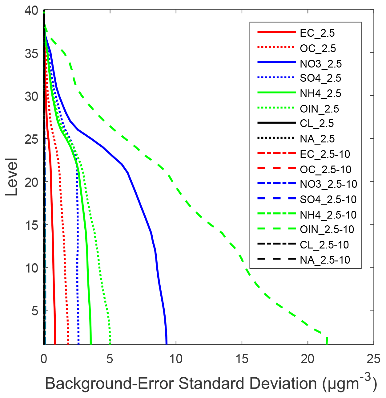
The MOSAIC_4bins aerosol scheme adopted in this study accommodated eight aerosol types, namely, black ∕ elemental carbon (EC ∕ BC), organic carbon (OC), sulfates (SO), nitrates (NO), ammonium salts (NH), chlorides (Cl−), sodium salts (Na+), and other unclassified inorganic compounds (OIN). There were four particle-size bins (4bins) for each aerosol type, namely, 0.039–0.1, 0.1–1.0, 1.0–2.5, and 2.5–10 µm. Thus, there were 32 model variables that represented the various aerosols. However, limitations in computer memory and computational capacity necessitated a reduction in the total number of control variables. In addition, the AECs of fine (PM2.5) and coarse (PM2.5−10) particles differed significantly. Thus, two control variables for each aerosol type were designed – one corresponding to fine particles (formed by combining the first three particle-size bins) and one corresponding to coarse particles (the fourth particle-size bin). Thus, there were 16 control variables in the DA scheme, namely, EC2.5, EC2.5−10, OC2.5, OC2.5−10, SO, SO42.5−10, NO, NO32.5−10, NH, NH42.5−10, CL2.5, CL2.5−10, NA2.5, NA2.5−10, OIN2.5, and OIN2.5−10.
There were two problems associated with calculations involving B:
-
In this scheme, B contained 3.5×10¹⁴ (square of 16 (number of control variables) (number of grid cells)) elements. Thus, it was necessary to mathematically treat and simplify B to facilitate numerical calculations. Following the method used by Li et al. (2013) and Zang et al. (2016), B was decomposed into a background-error standard deviation (BESD) matrix, a background-error horizontal correlation coefficient (BEHCC) matrix, and a background-error vertical correlation coefficient (BEVCC) matrix for calculations.
-
As the true value of B was unknown, it was necessary to develop a reasonable statistical method to estimate it. The National Meteorology Center (NMC) method (Parrish and Derber, 1992) was employed in this study to statistically estimate B. Specifically, the differences between the 48 and 24 h forecasts of the control variables were assumed to be a proxy of the background error. Next, B was estimated based on the covariance of the difference field, which was obtained by producing continuous 24 and 48 h forecasts for a month using the WRF–Chem model.
2.5 Observation operator and its adjoint
Obtaining the observation operator involved two calculations:
-
The control variables at each grid cell were mapped to the observation space; that is, the control variables were mapped to the AEC values (or PM2.5 and PM10 MCs).
-
The mapped values at the eight vertices of the model grid cell associated with the observation data were interpolated using the inverse distance-weighted method to the observation location. Here, we only describe the first step of the derivation of the observation operators, which are different for different observation data.
The AEC observation operator was based on the IMPROVE equation. The following shows the specific form of the IMPROVE equation:
The left side of Eq. (2) is the AEC value Ext (unit: 10−6 m−1). The variables in the brackets on the right side of Eq. (2) are combinations of the 16 control variables (unit: µg m−3). The coefficient variables fs(RH), fl(RH), and fss(RH) reflect the effects of hygroscopicity of fine, coarse, and sea-salt aerosols, respectively, under various relative humidity (RH) conditions. The values of the parameters given by Gordon et al. (2018) were used in this study. The variables (in square brackets) at each grid cell were obtained by combining the 16 control variables using the following method:
The principle for determining α involved preferentially allocating NH to SO. The remaining NH was allocated to NO.
The observation operators for PM2.5 and PM10 were the sums of control variables in the corresponding particle-size bin, that is,
The corresponding adjoint process on the operators for PM and AEC were developed and passed the adjoint sensitivity test. For the adjoint test method, please refer to Zou et al. (1997).
2.6 DA and forecast experimental design and verification analysis method
To analyze the effects of DA on aerosol analysis and forecasts, one control experiment and three DA experiments were designed for a pollution event that occurred from 13 to 14 November 2018 (Table 1). In the control experiment, no chemical observation data were assimilated. Forecasts were produced for a 36 h period, starting at 00:00 UTC on 13 November 2018. In the DA experiments, aerosol data were assimilated every hour for the DA period of 00:00–12:00 UTC on 13 November 2018. Next, with the analysis field obtained from the DA as the initial chemical field, forecasts were performed for a 24 h period starting at 12:00 UTC on 13 November 2018. For the first DA cycle in each of the three DA experiments, the initial field of the control experiment was used as the background field, the observation data for 00:00 UTC on 13 November 2018 were assimilated, and a DA analysis field was generated. With this DA analysis field as the initial field at 00:00 UTC on 13 November 2018 in the DA experiment, 1 h forecasts were produced. The forecasts produced for 01:00 UTC on 13 November 2018 were used as the background field for the second DA cycle. The process was repeated for 13 assimilation cycles. Thus, a DA analysis field for 12:00 UTC on 13 November 2018 was generated. The effects of DA on forecast performance during the forecast comparison period from 12:00 UTC on 13 November 2018 to 12:00 UTC on 14 November 2018 were analyzed by comparing the forecast performance of the DA and control experiments. In the first DA experiment, PM data alone were assimilated (DA_PM). In the second DA experiment, the lidar data alone were assimilated (DA_Ext). In the third DA experiment, PM and lidar data were assimilated simultaneously (DA_PM_Ext). Furthermore, 6 h reanalysis data provided by the US National Centers for Environmental Prediction (NCEP) were used as the meteorological field of the model.
Two metrics, the regional mean and root-mean-square error (RMSE), were used to evaluate simulation and forecast accuracy of the PM2.5 MC in the experiments. The closer the mean of the simulated values to the mean of the measurements and the smaller the RMSE, the higher the performance. Let Mi, Oi, N, , and be the simulated value sample, the measured value sample, the number of samples, the mean of simulated values, and the mean of the measurements, respectively. The following summarizes the equations for calculating the metrics:
3.1 BESD and BEVCC
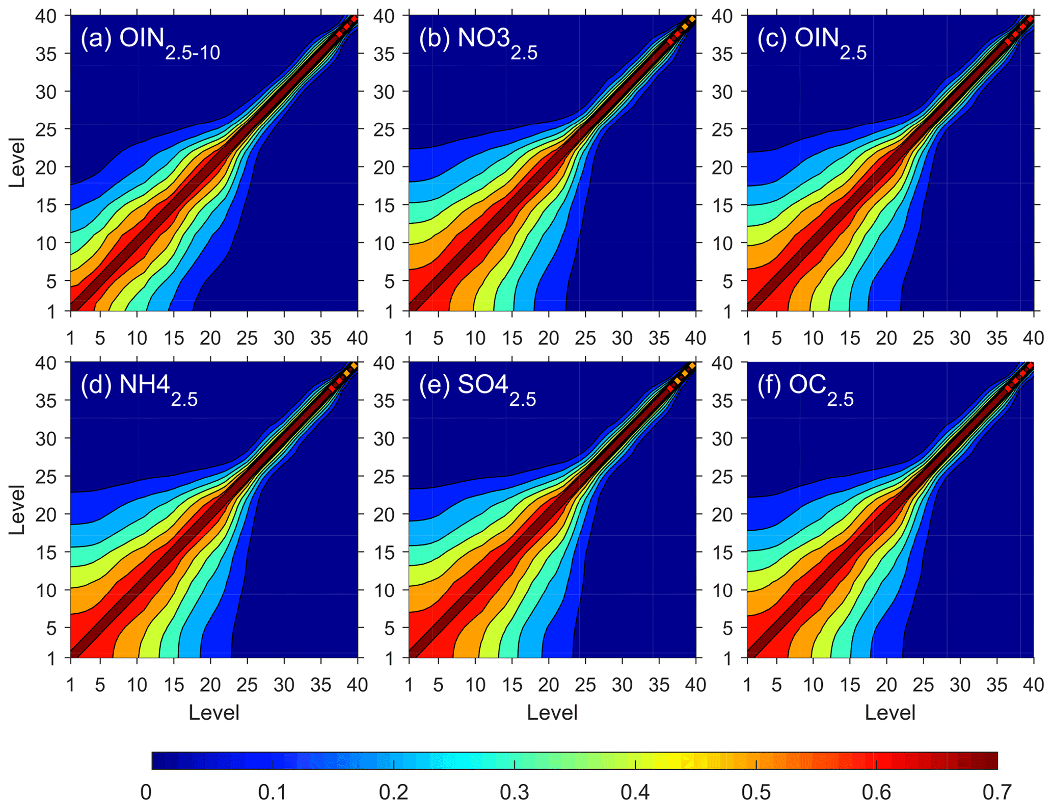
Under the same conditions, the larger the BESD, the larger the DA increment field (the difference between the “optimal” analysis field and the background field). Therefore, the structural pattern of the BESD significantly affected the distribution pattern of the DA increment field. The vertical BESD profiles of the 16 control variables are shown in Fig. 2. The BESD differed significantly among the control variables. The seven control variables with the largest BESDs below the height of 1000 m (corresponding to the 22nd layer of the model) in descending order of BESD were OIN2.5−10, NO, OIN2.5, NH, SO, OC2.5, and EC2.5. As height increased, the BESD of each control variable decreased. The rates of decrease were the highest above the boundary layers at heights of 1000–2000 m (corresponding to the 20th–25th layers of the model). The BEVCC matrix can spread the observation information contained in measurements around one model layer to nearby vertical layers. Therefore, even if the PM data are only available at the surface, there will still be increments of PM near the surface (in-air) after DA. Furthermore, even though the lidar AEC data are not available at the surface, assimilating lidar data can still correct the surface PM2.5 MC distribution. Figure 3 shows the BEVCC matrices of six control variables with relatively large BESDs (OIN2.5−10, NO, OIN2.5, NH, SO, and OC2.5). The BEVCCs of the six control variables share certain common characteristics. The correlation decreases as the interlayer spacing of the model increases. Each in-air layer is positively correlated with the surface layer, although the correlation decreases as height increases. For OIN2.5−10, the correlation coefficient between the surface and 10th layers is 0.34, compared with 0.49–0.51 for other variables. This indicates that OIN2.5−10 has a significantly weaker vertical correlation, and hence DA increments of these particles settle more rapidly than the other variables do. This is mainly because coarse particles settle faster vertically than fine particles and are concentrated near the surface in larger quantities.
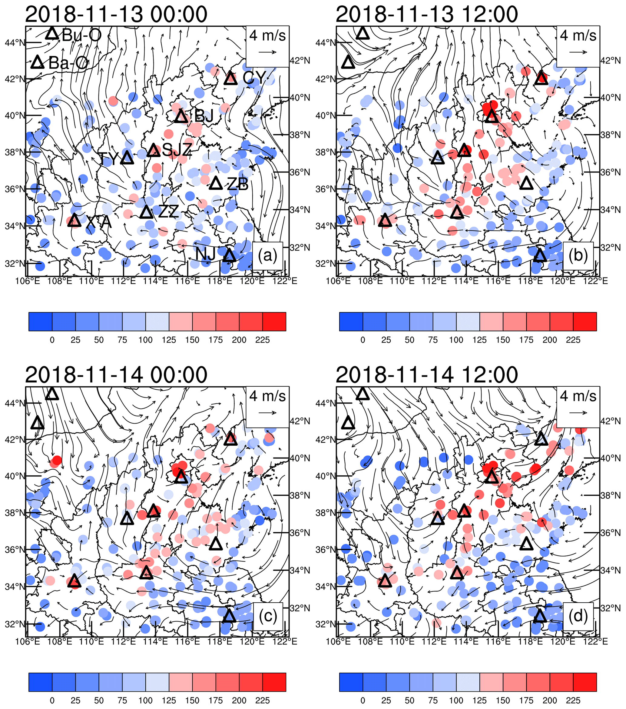
Figure 4Surface PM2.5 MC measurements in the D02 region and NCEP reanalysis wind field for the period from 00:00 UTC on 13 November 2018 to 12:00 UTC on 14 November 2018 (Bu-O: Buyant-Ovoo; Ba-O: Bayan-Ovoo; CY: Chaoyang; BJ: Beijing; SJZ: Shijiazhuang; TY: Taiyuan; ZB: Zibo; X'A: Xi'an; ZZ: Zhengzhou; NJ: Nanjing).

Figure 5AEC profiles measurements (black lines), the AEC profiles in the analysis fields of the control (blue lines), DA_PM (green lines), DA_Ext (purple lines), and DA_PM_Ext (red lines) experiments and the simulated RH profiles (orange lines) at four lidar stations at 00:00 UTC on 13 November 2018 (BJ: Beijing; SJZ: Shijiazhuang; TY: Taiyuan; WH: Wuhu).
3.2 Analysis of the pollution process
Figure 4 shows the evolutionary process of the surface PM2.5 MC and the NCEP reanalysis surface wind field in the D02 region for the period from 00:00 UTC on 13 November 2018 to 12:00 UTC on 14 November 2018 (the time interval between Fig. 4a–d is 12 h). At 00:00 UTC on 13 November 2018, the D02 region was predominantly controlled by a high-pressure circulation centered over Zibo. There was a clockwise wind field around the high-pressure center. Therefore, the northerlies (easterlies) east (south) of the high-pressure center brought clean air over the sea land-ward. As a result, the PM2.5 MCs over East China were relatively low. For example, the mean PM2.5 MC measured at the ground environmental monitoring stations in Nanjing was 41.8 µg m−3. There were relatively slow southerlies west and northwest of the high-pressure center, which led to favorable conditions for pollutant accumulation east of the Taihang Mountains and south of the Yan Mountains. As a result, North China was heavily polluted by PM2.5. For example, the mean PM2.5 MCs in Beijing and Shijiazhuang were 122.7 and 149.3 µg m−3, respectively. In addition, within the D02 region, there was a northeast–southwest-trending cold front near Buyant-Ovoo–Bayan-Ovoo in Mongolia. As time passed (Fig. 4b–d), the high-pressure center gradually moved northeastward and reached near the eastern boundary of the D02 region by 12:00 UTC on 14 November 2018 (Fig. 4d). The cold front gradually moved southeastward and reached the Chaoyang–Beijing–Taiyuan–Xi'an line by 12:00 UTC on 14 November 2018 (Fig. 4d). As the high-pressure center and the cold front moved, the level of pollution in North China continued to rise, and pollution gradually expanded northeastward to Chaoyang, southward to Zhengzhou, and westward to Taiyuan. The level of pollution gradually increased in the Wei and Yellow river valleys east of Xi'an due to the dual action of advection by the easterlies and the narrow terrain, while the PM2.5 MCs decreased considerably with the passing of the cold front due to the good dispersion conditions. There were no significant changes in the PM2.5 MCs in East China due to the continuous impact of sea winds.
3.3 Analysis of the direct effects of DA
Figure 5 shows the AEC profile measurements, the AEC profiles in the analysis fields of the control and DA experiments, and the simulated RH profiles at four lidar stations at 00:00 UTC on 13 November 2018, when the first DA cycle was performed. The results of the control experiment were used as the background field in the three DA experiments. Figure 5a–d show the results for Beijing, Shijiazhuang, Taiyuan, and Wuhu, respectively. As the in-air RH profile (brown lines) below 1 km was basically consistent with that of the surface RH, the vertical changes in the AEC values in this region were only slightly affected by the RH. Thus, the AEC profiles were used to study the vertical changes in the PM2.5 MC. For Beijing, the simulated AEC results from the control experiment (blue lines) agreed with the lidar AEC measurements well (Fig. 5a – black lines). However, for Shijiazhuang and Taiyuan, the simulation underestimated the empirical results (Fig. 5b and c, respectively), particularly near the height of 100 m (the lowest height of valid lidar data), while for Wuhu, it overestimated them (Fig. 5d).
The DA increments of AEC values from the DA_PM, that is, the AEC values obtained from the DA_PM experiment (green lines) minus those from the control experiment (blue lines), were negative for Beijing (Fig. 5a), Taiyuan (Fig. 5c), and Wuhu (Fig. 5d) at the surface. They were also negative from the near-surface to a height of about 1000 m, although their absolute values were smaller than those at the surface. This is because the BEVCCs between each in-air layer and the surface layer were positive and decreased with height (Fig. 3) so that the information contained in the surface PM MC measurements was spread to the air. However, the results of the adjustment of the AEC profiles were not always positive, because the aerosol bias of the control experiment at the surface was not always the same as it was in the atmosphere. Thus, they were overall positive for Beijing and Wuhu but negative for Taiyuan, reflecting the fact that the PM DA did not effectively account for the vertical aerosol distribution adjustment.
Compared to those from the DA_PM experiments, the AEC values from the DA_Ext experiments (purple lines) for Taiyuan (Fig. 5c) at heights of approximately 100 and 700 m were significantly larger than those from the DA_PM experiment and were consistent with the measurements (black line), and those for Wuhu (Fig. 5d) were very close to the measurements across the entire profile. This suggests that the AEC observation operator whose design was based on the IMPROVE equation effectively facilitated 3D variational assimilation of lidar AEC data. In addition, although lidar data were not available at the surface, the DA_Ext adjusted the surface PM MCs, corrected the overestimation of surface PM2.5 MCs in Beijing and Wuhu but increased the overestimation of surface PM2.5 MCs in Taiyuan. This is because the information contained in the in-air AEC was spread to the surface, while the aerosol bias of the control experiment in the air did not always match that at the surface.
The in-air AEC profiles obtained from the DA_PM_Ext experiment (red lines) for the four cities almost coincided with those from the DA_Ext experiments above 400 m. The near-surface AEC values obtained from the DA_PM_Ext experiment for Beijing (Fig. 5a), Taiyuan (Fig. 5c), and Wuhu (Fig. 5d) almost coincided with those from the DA_PM experiment, were between those from the DA_PM and DA_Ext experiments, and were smaller than those from both the DA_PM and DA_Ext experiments. This suggests that simultaneously assimilating the two types of data can fully integrate their observation information and reflect their respective advantages, thereby generating the most accurate analysis field.
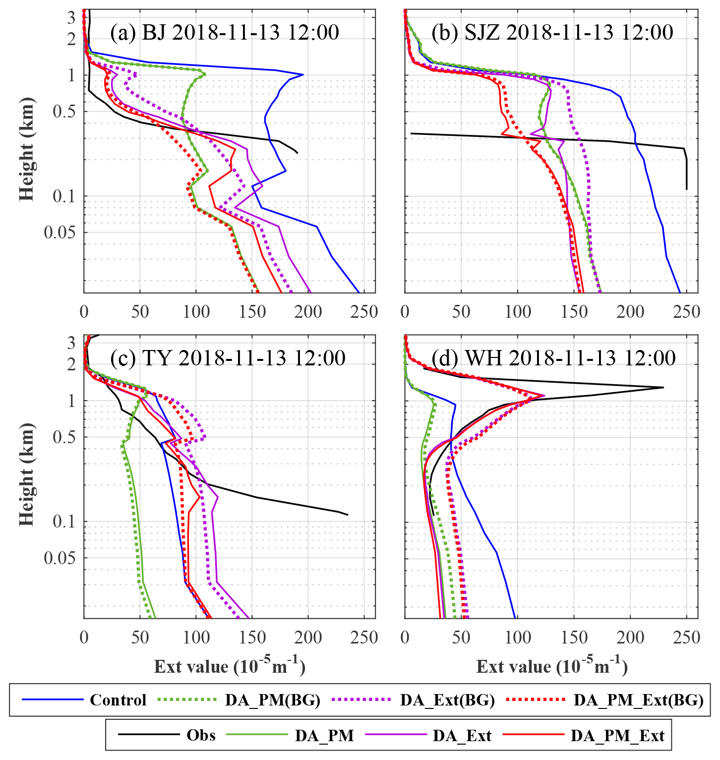
Figure 6AEC profiles measurements (solid black lines), the AEC profiles in the control experiment (solid blue lines), in the background field of the DA_PM (dotted green lines), DA_Ext (dotted purple lines), and DA_PM_Ext (dotted red lines) experiments, and in the analysis fields of the DA_PM (solid green lines), DA_Ext (solid purple lines), and DA_PM_Ext (solid red lines) experiments at four lidar stations at 12:00 UTC on 13 November 2018 (BJ: Beijing; SJZ: Shijiazhuang; TY: Taiyuan; WH: Wuhu).
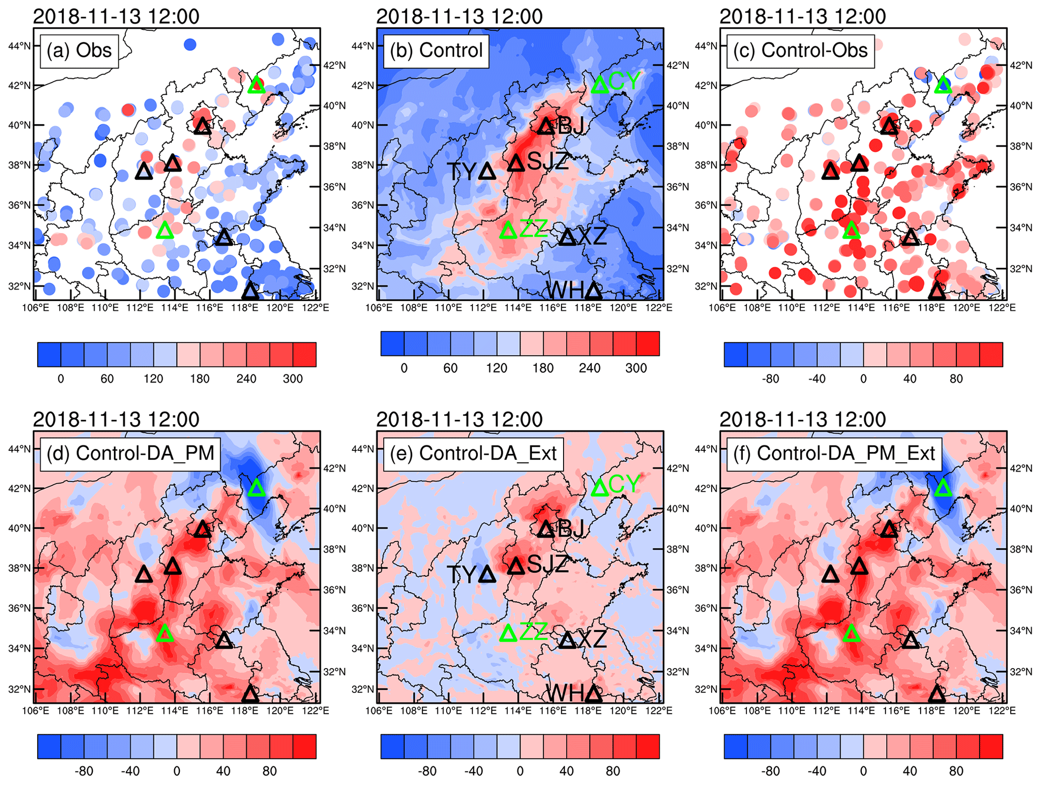
Figure 7Surface PM2.5 MC measurements (a), surface PM2.5 MCs in the initial field of control experiment (b) and its bias (c), the inverse DA increments of PM2.5 MC of DA experiments, that is, the PM2.5 MCs obtained from the control experiment minus that from the DA experiments (d–f) at 12:00 UTC on 13 November 2018 (black triangles signify the locations of the lidar stations, and green triangles mark the locations of the two cities without lidar) (CY: Chaoyang; BJ: Beijing; SJZ: Shijiazhuang; TY: Taiyuan; ZZ: Zhengzhou; XZ: Xuzhou; WH: Wuhu).
Figure 6 shows the AEC profiles measured, simulated by the control experiment, in the background fields and the analysis fields of the DA experiments at four lidar stations at 12:00 UTC on 13 November 2018. The time of 12:00 UTC on 13 November 2018 was the last time point of the DA period, the starting time point of the forecast period, and the time point at which 13 DA cycles had elapsed. The background field for each of the three DA experiments was generated during the continuous DA period, whereas the results of the control experiment were obtained by a 12 h forecast starting at 00:00 UTC on 13 November 2018. As a result, there was a significant difference between the background fields of the three DA experiments and those of the control experiment.
The DA increments of the AEC values from the DA_PM experiment were significant below 1000 m (green lines). These adjustments corrected the near-surface overestimation of the AEC values for the four cities in the control experiment; however, they increased the underestimation for Taiyuan at heights of 120–400 m (Fig. 6c) and overestimation for Wuhu above 400 m (Fig. 6d). Additionally, it is worth noting that there were small direct DA increments generated in the DA_PM experiment at this time point. This means that for the surface PM DA, a DA period of 11 h or less was sufficient to effectively adjust aerosol distribution in this experiment. This may be because aerosols were primarily concentrated near the surface and surface PM data covered a wide area and had a high spatial resolution. Thus, surface PM data measured at a few time points contained the main aerosol distribution information for the whole region.
Compared to the DA_PM experiment, the DA_Ext experiment (purple lines) reflected the advantages of adjusting the vertical aerosol distribution. The overestimations for Beijing above 300 m (Fig. 6a), Taiyuan above 600 m (Fig. 6c), and Wuhu below 400 m (Fig. 6d) in the control experiment were effectively corrected. The rapid decrease in the AEC from the surface to a height of 1000 m over Beijing (Fig. 6a) and the maximum-AEC layer at a height of 1300 m over Wuhu (Fig. 6d) were accurately reproduced by the DA_Ext experiment. However, the near-surface overestimation for Taiyuan (Fig. 6c) increased. Moreover, the direct DA increments generated in the DA_Ext experiment at this time point remained notable. This suggests that the background field errors at each lidar station at 12:00 UTC remained relatively large, even after the continuous DA period. To improve the effects of the DA, it was necessary to increase the length of the continuous DA period. This may have been due to the limited number of lidars and the fact that the lidars were relatively far apart from one another. Thus, the simulation error for the region upstream of a lidar was difficult to correct through DA and affected the lidar location due to the effects of advection at the next time point. In addition, because the 12:00 UTC (20:00 LST) was only 2–3 h after sunset, large changes of PM concentration profile may occur due to large changes in the planetary boundary layer height after sunset.
Figure 7 shows the surface PM2.5 MC measurements, the surface PM2.5 MCs of the initial field of the control experiment and their biases, and the inverse DA increments of PM2.5 MCs from the DA experiments, that is, the PM2.5 MCs obtained from the control experiment minus those from the DA experiments at 12:00 UTC on 13 November 2018. The measurements (Fig. 7a) showed that the PM2.5 MCs were relatively high in North China, with a heavily polluted zone in the Beijing–Shijiazhuang–Zhengzhou region, while the PM2.5 MCs were relatively low surrounding North China. The control experiment (Fig. 7b) successfully simulated regions with relatively high and low PM2.5 MCs. However, the PM2.5 MCs were overestimated for most stations in D02 (Fig. 7c), especially in the Beijing–Shijiazhuang–Zhengzhou region, and underestimated for stations near Chaoyang.
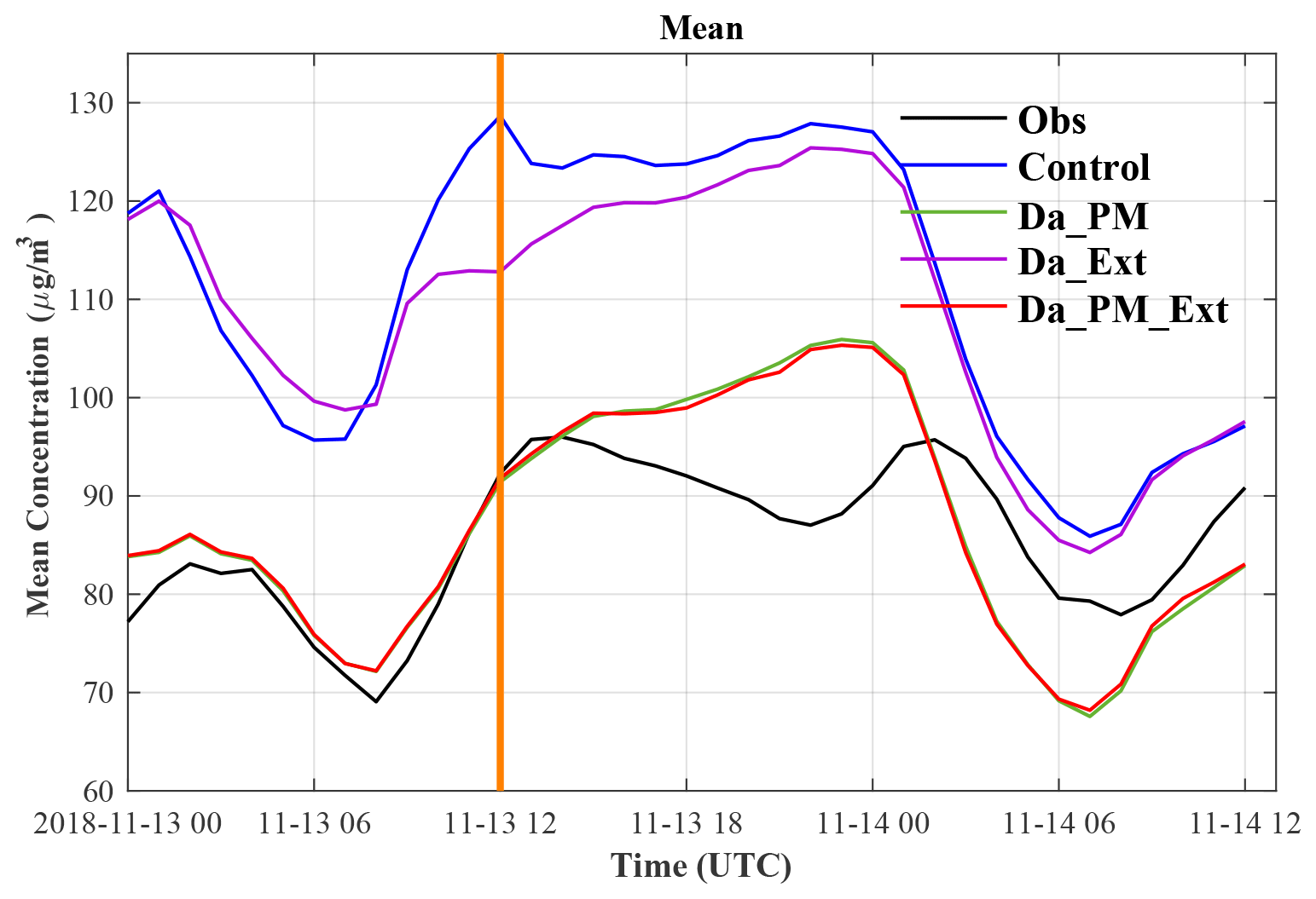
Figure 8Variation of the regional mean PM2.5 MC over time measured and simulated by the four experiments (the vertical orange line separates the DA and forecast periods; the black line signifies measurements; the blue line signifies that obtained from the control experiment; the green, purple, and red lines signify that obtained from the DA_PM, DA_Ext, and DA_PM_Ext experiments, respectively).
The inverse DA increments of the PM2.5 MCs of the DA_PM experiment (Fig. 7d) were relatively consistent with the bias of the control experiment (Fig. 7c), indicating that the overestimation for most regions and the underestimation for some regions in the initial field of the control experiment were corrected by the PM DA. The inverse DA increments of the PM2.5 MCs of DA_Ext (Fig. 7e) were significant in the regions surrounding and downstream of the five lidar stations. In addition, certain DA increments were also present in regions far away from the lidar stations. This indicates that long-term continuous lidar AEC DA can affect a relatively large area. Overall, the DA_Ext corrects the overestimation for most stations and underestimation for a few stations in the control experiment. However, the DA_Ext increments were smaller than the DA_PM increments in terms of horizontal spatial range and absolute values. This is mainly because there are relatively few lidars, and these lidars cover a limited spatial area. It is worth noting that DA_Ext yields a negative effect for northern Beijing and the region around Taiyuan, a result which will be discussed later in Sect. 4. The inverse DA increments of PM2.5 MCs of DA_PM_Ext (Fig. 7f) were relatively consistent with those of the DA_PM (Fig. 7c). This is mainly because the quantity and spatial coverage of the PM data were larger and more complete than those of the lidar data. As a result, the DA increments of the surface PM2.5 MCs originated primarily from the observation information contained in the PM data. Because the AEC profiles of the DA_PM_Ext almost coincided with those of the DA_Ext above 400 m (Fig. 5), the DA_PM_Ext reflected the 3D spatial distribution pattern of the aerosols most accurately.
3.4 Effects of DA on the forecast performance for surface PM2.5 MCs
In this section, the forecast performances of the DAs for surface PM2.5 are evaluated based on measurements that cover most of the D02 region.
Figure 8 shows the variation of the regional mean of the PM2.5 MC over time from the four experiments. The regional mean of the PM2.5 MC (black line) exhibited a notable diurnal pattern. Two notable minimum PM2.5 MC values (69.1 and 77.9 µg m−3) appeared at 08:00 UTC (16:00 local time) on 13 and 14 November 2018, respectively. High PM2.5 MCs appeared between 13:00 UTC on 13 November 2018 and 02:00 UTC on 14 November 2018 (from night to morning), with a maximum PM2.5 MC of 96.0 µg m−3. Meanwhile, there was a relative minimum PM2.5 MC (87.0 µg m−3) appearing at 22:00 UTC on 13 November 2018 (around dawn local time) during the high-PM2.5-MC period.
The control experiment (blue line) simulated the periodic variation pattern of the mean PM2.5 MC but significantly overestimated the value of this parameter during the entire forecast period. The mean PM2.5 MC of the control experiment at the initial time for the forecast period (12:00 UTC on 13 November 2018) was 128.6 µg m−3, which is 36.3 µg m−3 (39.3 %) larger than that of the measurements (92.3 µg m−3). The DA_PM (green line, which almost coincides with the red line) significantly reduced the overestimation of the control experiment, with a mean PM2.5 MC of 91.4 µg m−3 that is 0.9 µg m−3 (1.0 %) lower than the measurement. As a result of the decrease in the MC levels in the initial field, the PM2.5 MC forecasts of the DA_PM were significantly lower than those of the control experiment during the entire forecast period. This suggests that the overestimation of the initial field is the primary cause of the overestimated forecasts of the control experiment. The overestimation of the control experiment at the initial time point was reduced by the DA_Ext (purple line) from 36.3 µg m−3 (39.3 %) to 20.5 µg m−3 (22.2 %), which improved the forecast performance significantly (even though there were only five lidars within the region). There was no significant difference between the results of the DA_PM_Ext (red line) and DA_PM (green line) at the surface. This suggests that in these experiments, after DA of surface PM data, the DA of lidar data did not significantly affect the surface PM2.5 MC levels. There are two reasons for this. The PM data set was far larger than the lidar data set in terms of quantity and spatial coverage. In addition, after surface PM DA, lidar DA mainly directly adjusted the AMC values not at surface but in-air and hence affected the surface AMC forecasts only indirectly, via processes such as settling. However, in this simulation process, the surface AMC levels remained relatively high, while the vertical air movement was weak due to the relatively stable meteorological conditions, particularly in the heavily polluted zone. Therefore, the effects of the lidar DA on the surface PM2.5 MCs are far smaller after the surface PM DA.
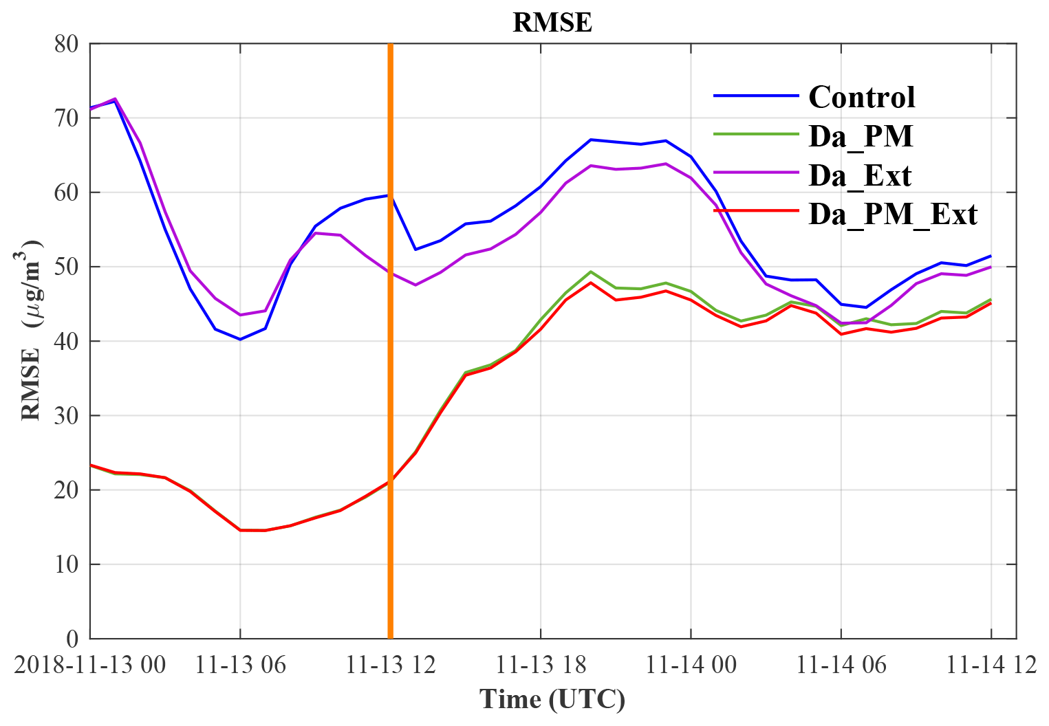
Figure 9Variation in the RMSE of surface PM2.5 MC forecasts over time (the vertical orange line separates the DA and forecast periods; the blue line signifies that obtained from the control experiment; the green, purple, and red lines signify that obtained from the DA_PM, DA_Ext, and DA_PM_Ext experiments, respectively).
Figure 9 shows the variation in the RMSE of surface PM2.5 MC forecasts over time. The RMSEs for simulations and forecasts were relatively large (small) when the mean PM2.5 MCs were relatively high (low) (Fig. 8). The RMSE in the control experiment was 59.6 µg m−3 at the initial time for the forecast period (12:00 UTC on 13 November 2018) and fluctuated between 44.5 and 67.1 µg m−3 instead of linearly increasing or decreasing throughout the forecast period. The RMSEs in the DA_PM (green line), DA_Ext (purple line), and DA_PM_Ext (red line) experiments at the initial time point were 21.0, 49.1, and 21.2 µg m−3, respectively, which were 38.6 µg m−3 (64.8 %), 10.5 µg m−3 (17.6 %), and 38.4 µg m−3 (64.4 %) lower than that of the control experiment. Owing to the optimized initial field, the RMSE of the forecasts of each of the DA experiments was lower than that of the control experiment during the forecast period. For the 24th forecast hour, the RMSEs of the forecasts of the Da_PM, Da_Ext, and DA_PM_Ext were 6.1 µg m−3 (11.8 %), 1.5 µg m−3 (2.9 %), and 6.5 µg m−3 (12.6 %) smaller than that of the control experiment, respectively. This suggests that the optimization of the initial field has a lasting (more than 24 h in all cases) positive effect on model forecasts. It is worth noting that while there are very few lidar stations, the results of the DA_Ext experiment were still better than those of the control experiment, and the results of the DA_PM_Ext experiment were also slightly better than those of the DA_PM experiment. This indicates that even in relatively low quantities, lidar data still improve the forecast performance of the model. As lidar data become increasingly rich and provide more vertical and horizontal aerosol distribution information in the future, lidar DA will further improve PM2.5 MC forecasts.
DA_Ext had a negative effect on the surface PM2.5 MC distributions for regions around Taiyuan and northern Beijing (Fig. 7e). For Taiyuan, the cause of the negative effect was similar to that responsible for the results shown in Fig. 5; that is, the information contained in the in-air AEC was spread to the surface by DA_Ext. However, the AEC showed an underestimation bias of the control experiment at a height of 100 m, while the PM MC measurements showed an overestimation bias at the surface. There are two reasons for the differences between the bias of the control experiment in-air and at surface, as reflected by the AEC and PM MC measurements. First, it is not abnormal for the simulation error of the model to differ in the vertical direction due to the complex evolution mechanism of aerosols, which we do not discuss here. Second, the PM2.5 MCs measured at 12:00 UTC on 13 November 2018 at three ground environmental monitoring stations within 6 km of the Taiyuan lidar station were 80.0, 137.0, and 146.0 µg m−3, respectively, indicating a large horizontal gradient of AMC and PM MC around the Taiyuan lidar station. Therefore, the observation information contained in the lidar profile did not represent the spatial distribution well and differed significantly from that contained in the PM data nearby. This suggests that the spatial representation of lidar data could significantly affect the impact of the lidar AEC DA. In addition, the vertical resolution of the lidar data (smaller than 15 m) is far smaller than the spacing between adjacent height layers of the model. As a result, the representative spatial scale of the original lidar data does not match the resolution of the model. To improve the accuracy of the horizontal spatial representativeness of the lidar data, at each time point, the lidar AEC profile was based on hourly averaged lidar data (from the previous hour). The vertical spatial representativeness of the data was improved by smoothing over 30 m in the vertical direction. However, the time-averaged lidar data represented observation information for a certain area downstream of the wind field. These errors need to be addressed in subsequent studies. Moreover, the selection of a time-averaging period and vertical smoothing length also requires further investigation.
For northern Beijing, the underestimation resulted primarily from the notable Beijing lidar overestimation, whereas the overestimation was relatively small in northern Beijing, the downstream region of the Beijing lidar. In addition, there was even underestimation in some of the PM measurement stations north of Beijing (Fig. 7c). Therefore, the downstream transference of lidar DA information from Beijing lidar location to northern Beijing caused the underestimation in the continuous DA results. The most direct and effective measure for addressing this problem is to increase the number of lidars and the coverage of the lidar network. This measure will ensure that the simulation bias for the simulation region will be more comprehensively captured. However, lidar detection requires large amounts of labor and financial resources. Therefore, it is difficult to arrange lidar stations as densely as ground environmental monitoring stations. A relatively feasible method is to set a relatively small number of lidars in regions with a relatively uniform simulation bias and set dense lidars in regions where the simulation bias changes significantly. This will make it possible to use a limited number of lidars to capture more useful information. Thus, studying the temporal and spatial distribution of model simulation bias can provide a useful reference for the future arrangement and planning of the lidar stations. This merits further investigation.
The AEC observation operator used in this study was designed based on the IMPROVE equation, with parameters such as the hygroscopicity coefficient set to values reported in previous studies. On the one hand, data sets from which the IMPROVE parameters were determined in previous studies were measured in specific regions and near the ground. The verification of the IMPROVE parameters had not been thoroughly conducted for the locations where lidar data were provided. Therefore, there may have been different biases between the Mie algorithm and the IMPROVE algorithm in different regions, inducing inconsistent assimilation performance. Additionally, the values of the coefficients in the IMPROVE equation were determined by statistical analysis of extensive data. This dictated that these coefficients represented average levels under certain pollution and humidity conditions. There may be certain biases in these coefficients when applied to a specific observation event. These biases will accumulate and amplify during the calculation of the forward and adjoint processes of the observation operator, resulting in a negative effect DA effect. Hence, another issue needing to be addressed is how to effectively evaluate the applicability of the IMPROVE equation and more accurately adjust its coefficients.
In this study, an observation operator and its adjoint for the AEC DA were designed based on the IMPROVE equation, and a 3-DVAR DA system was developed for lidar AEC data and surface AMC data for the MOSAIC_4bin chemical scheme in the WRF–Chem model. Three DA experiments (i.e., a PM2.5 (PM10) DA experiment, a lidar AEC DA experiment, and a simultaneous PM2.5 (PM10) and lidar AEC DA experiment) were conducted based on AEC profiles captured by five lidars (located in Beijing, Shijiazhuang, Taiyuan, Xuzhou, and Wuhu) as well as PM2.5 and PM10 measurements taken at over 1500 ground environmental monitoring stations across China in the period from 00:00 to 12:00 UTC on 13 November 2018. A comparison with the control experiment involving no DA found that the 3-DVAR DA system was effective at assimilating lidar AEC data. While there were only five lidars within the simulation region (approximately 2.33 million km2 in size), assimilating AEC data alone was still found to effectively improve the accuracy of the initial field, hence improving the forecast performance for PM2.5 for more than 24 h. The lidar AEC DA can reduce the RMSE of the surface PM2.5 MC in the initial field of the model by 10.5 µg m−3 (17.6 %). In addition, a 38.4 µg m−3 (64.4 %) reduction occurred when the PM2.5 (PM10) and lidar AEC data were assimilated simultaneously. The RMSEs of the forecasted surface PM2.5 MC 24 h after the DA period in the three DA experiments were reduced by 6.1 µg m−3 (11.8 %), 1.5 µg m−3 (2.9 %), and 6.5 µg m−3 (12.6 %), respectively. Lidar AEC DA was advantageous for improving the accuracy of the vertical PM2.5 MC profile. Surface PM2.5 (PM10) DA was advantageous for optimizing the near-surface PM2.5 MC distribution. Simultaneous lidar AEC and surface PM2.5 (PM10) DA effectively integrated their observation information to generate a more accurate 3D aerosol analysis field.
The WRF–Chem model source code can be downloaded at the WRF model download page (https://www2.mmm.ucar.edu/wrf/users/download/get_source.html, last access: 24 August 2020). This 3-DVAR data assimilation system was developed by the authors. The code of this system can be obtained on request from the corresponding author (ywlx_1987@163.com and zzlqxxy@163.com). Aerosol lidar data can be obtained on request from the first author (13270805867@163.com).
YL performed numerical experiments, analyzed the data, and wrote the initial manuscript. YL, ZZ, and WY developed the 3-DVAR data assimilation system, designed this study, and revised the manuscript. ZZ supervised the project of development. DL provided the lidar observation data in four sites. All the authors continuously discussed the 3-DVAR system development and the results of the manuscript.
The authors declare that they have no conflict of interest.
We thank the China National Environmental Monitoring Center (CNEMC) for providing PM2.5 and PM10 data through their website (http://www.cnemc.cn/, last access: 29 September 2020).
This research was primarily supported by the National Key Research and Development Program of China, (grant no. 2017YFC1501702) and the National Natural Science Foundation of China (grant nos. 41775123 and 41805092).
This paper was edited by Samuel Remy and reviewed by two anonymous referees.
Bannister, R. N.: A review of operational methods of variational and ensemble-variational data assimilation, Q. J. Roy. Meteor. Soc., 143, 607–633, https://doi.org/10.1002/qj.2982, 2017.
Baraskar, A., Bhushan, M., Venkataraman, C., and Cherian, R.: An offline constrained data assimilation technique for aerosols: Improving GCM simulations over South Asia using observations from two satellite sensors, Atmos. Environ., 132, 36–48, https://doi.org/10.1016/j.atmosenv.2016.02.026, 2016.
Benedetti, A., Morcrette, J. J., Boucher, Dethof, O., Engelen, R. J., Fisher, M., Flentje, H., Huneeus, N., Jones, L., Kaiser, J. W., Kinne,S., Mangold, A., Razinger, M., Simmons, A. J., and Suttie, M.: Aerosol analysis and forecast in the European Centre for Medium-Range Weather Forecasts Integrated Forecast System: 2. Data assimilation, J. Geophys. Res., 114, D13205, https://doi.org/10.1029/2008JD011115, 2009.
Burton, S. P., Ferrare, R. A., Hostetler, C. A., Hair, J. W., Kittaka, C., Vaughan, M. A., Obland, M. D., Rogers, R. R., Cook, A. L., Harper, D. B., and Remer, L. A.: Using airborne high spectral resolution lidar data to evaluate combined active plus passive retrievals of aerosol extinction profiles, J. Geophys. Res.-Atmos., 115, D00H15, https://doi.org/10.1029/2009JD012130, 2010.
Cao, J. J., Wang, Q. Y., Chow, J. C., Watson, J. G., Tie, X. X., Shen, Z. X., Wang, P., and An, Z. S.: Impacts of aerosol compositions on visibility impairment in Xi'an, China, Atmos. Environ., 59, 559–566, https://doi.org/10.1016/j.atmosenv.2012.05.036, 2012a.
Cao, J. J., Shen, Z. X., Chow, J. C., Watson, J. G., Lee, S. C., Tie, X. X., Ho, K. F., Wang, G. H., and Han, Y. M.: Winter and Summer PM2.5 Chemical Compositions in Fourteen Chinese Cities, J. Air. Waste. Manage., 62, 1214–1226, https://doi.org/10.1080/10962247.2012.701193, 2012b.
Carmichael, G. R., Sandu, A., Chai, T., Daescu, D. N., Constantinescu, E. M., and Tang, Y.: Predicting air quality: Improvements through advanced methods to integrate models and measurements, J. Comput. Phys., 227, 3540–3571, https://doi.org/10.1016/j.jcp.2007.02.024, 2008.
Cheng, X. H., Liu, Y. L., Xu, X. D., You, W., Zang, Z. Z., Gao, L. N., Chen, Y. B., Su, D. B., and Yan, P.: Lidar data assimilation method based on CRTM and WRF-Chem models and its application in PM2.5 forecasts in Beijing, Sci. Total. Environ., 682, 541–552, https://doi.org/10.1016/j.scitotenv.2019.05.186, 2019.
Chen, Y., Li, F. F., Shao, N., Wang, X. P., Wang, Y. M., Hu, X. Y., and Wang, X.: Aerosol Lidar Intercomparison in the Framework of the MEMO Project. 1. Lidar Self Calibration and 1st Comparison Observation Calibration Based on Statistical Analysis Method, in: 2019 International Conference on Meteorology Observations (ICMO), Chengdu, China, 28–31 December 2019, 1–5, https://doi.org/10.1109/ICMO49322.2019.9026086, 2019.
Chen, Z. J., Zhang, J. S., Zhang, T. S., Liu, W. Q., and Liu, J. G.: Haze observations by simultaneous lidar and WPS in Beijing before and during APEC, 2014, Sci. China. Chem., 58, 1385–1392, https://doi.org/10.1007/s11426-015-5467-x, 2015.
Ganguly, D., Ginoux, P., Ramaswamy, V., Dubovik, O., Welton, J., Reid, E. A., and Holben, B. N.: Inferring the composition and concentration of aerosols by combining AERONET and MPLNET data: Comparison with other measurements and utilization to evaluate GCM output, J. Geophys. Res.-Atmos. 114, D16203, https://doi.org/10.1029/2009JD011895, 2009.
Fernald, F. G.: Analysis of atmospheric lidar observations: some comments, Appl. Optics., 23, 652–653, https://doi.org/10.1364/AO.23.000652, 1984.
Gordon T. D., Prenni A. J., Renfro J. R., McClure, E., Hicks, B., Onasch, T. B., Freedman, A., McMeeking, G. R., and Chen, P.: Open-path, closed-path and reconstructed aerosol extinction at a rural site, J. Air. Waste. Manage., 68, 824–835, https://doi.org/10.1080/10962247.2018.1452801, 2018.
Haywood, J. and Boucher, O.: Estimates of the direct and indirect radiative forcing due to tropospheric aerosols: A review, Rev. Geophys., 38, 513–543, https://doi.org/10.1029/1999RG00:0078, 2000.
Jiang, Z. Q., Liu, Z. Q., Wang, T. J., Schwartz, C. S., Lin, H. C., and Jiang, F.: Probing into the impact of 3-DVAR assimilation of surface PM10 observations over China using process analysis, J. Geophys. Res.-Atmos., 118, 6738–6749, https://doi.org/10.1002/jgrd.50495, 2013.
Kahnert, M.: Variational data analysis of aerosol species in a regional CTM: background error covariance constraint and aerosol optical observation operators, Tellus B, 60, 753–770, https://doi.org/10.1111/j.1600-0889.2008.00377.x, 2008.
Kim, Y. J., Kim, K. W., Kim, S. D., Lee, B. K., and Han, J. S.: Fine particulate matter characteristics and its impact on visibility impairment at two urban sites in Korea: Seoul and Incheon, Atmos. Environ., 40, 593–605, https://doi.org/10.1016/j.atmosenv.2005.11.076, 2006.
Li, Z., Zang, Z., Li, Q. B., Chao, Y., Chen, D., Ye, Z., Liu, Y., and Liou, K. N.: A three-dimensional variational data assimilation system for multiple aerosol species with WRF/Chem and an application to PM2.5 prediction, Atmos. Chem. Phys., 13, 4265–4278, https://doi.org/10.5194/acp-13-4265-2013, 2013.
Liu, Q. H. and Weng, F. Z.: Advanced doubling-adding method for radiative transfer in planetary atmosphere, J. Atmos. Sci., 63, 3459–3465, https://doi.org/10.1175/JAS3808.1, 2006.
Liu, Z., Q. Liu, Q. H., Lin, H. C., Schwartz, C. S., Lee, Y. H., and Wang, T. J.: Three-dimensional variational assimilationof MODIS aerosol optical depth: Implementation and application to a dust storm over East Asia, J. Geophys. Res.-Atmos., 116, D23206, https://doi.org/10.1029/2011JD016159, 2011.
Lowenthal, D. H. and Kumar, N.: PM2.5 Mass and Light Extinction Reconstruction in IMPROVE, J. Air. Waste. Manage., 53, 1109–1120, https://doi.org/10.1080/10473289.2003.10466264, 2003.
Matthias, V., Freudenthaler, V., Amodeo, A., Balin, I., Balis, D., Bösenberg, J., Chaikovsky, A., Chourdakis, G., Comeron, A., Delaval, A., Tomasi, F. D., Eixmann, R., Hågård, A., Komguem, L., Kreipl, S., Matthey, R., Rizi, V., Rodrigues, J. A., Wandinger, U., and Wang, X.: Aerosol lidar intercomparison in the framework of the EARLINET project. 1. Instruments, Appl. Optics., 43, 961–976, https://doi.org/10.1364/AO.43.000961, 2004.
Milroy, C., Martucci, G., Lolli, S., Loaec, S., Sauvage, L., Xueref-Remy, I., Lavrič, J. V., Ciais, P., and O'Dowd, C. D.: On the ability of pseudo-operational ground-based light detection and ranging (LIDAR) sensors to determine boundary-layer structure: intercomparison and comparison with in-situ radiosounding, Atmos. Meas. Tech. Discuss., 4, 563–597, https://doi.org/10.5194/amtd-4-563-2011, 2011.
Niu, T., Gong, S. L., Zhu, G. F., Liu, H. L., Hu, X. Q., Zhou, C. H., and Wang, Y. Q.: Data assimilation of dust aerosol observations for the CUACE/dust forecasting system, Atmos. Chem. Phys., 8, 3473–3482, https://doi.org/10.5194/acp-8-3473-2008, 2008.
Parrish, D. F. and Derber, J. C.: The national meteorological center's spectral statistical-interpolation analysis system, Mon. Wea. Rev., 120, 1747–1763, https://doi.org/10.1175/1520-0493(1992)120<1747:TNMCSS>2.0.co;2, 1992.
Peng, Z., Liu, Z., Chen, D., and Ban, J.: Improving PM2.5 forecast over China by the joint adjustment of initial conditions and source emissions with an ensemble Kalman filter, Atmos. Chem. Phys., 17, 4837–4855, https://doi.org/10.5194/acp-17-4837-2017, 2017.
Pitchford, M., Maim, W., Schichtel, B., Kumar, N., Lowenthal, D., and Hand, J.: Revised algorithm for estimating light extinction from IMPROVE particle speciation data, J. Air. Waste. Manage., 57, 1326–1336, https://doi.org/10.3155/1047-3289.57.11.1326, 2007.
Raut, J.-C. and Chazette, P.: Assessment of vertically-resolved PM10 from mobile lidar observations, Atmos. Chem. Phys., 9, 8617–8638, https://doi.org/10.5194/acp-9-8617-2009, 2009.
Roy, B., Mathur, R., Gilliland, A. B., and Howard, S. C.: A comparison of CMAQ-based aerosol properties with IMPROVE, MODIS, and AERONET data, J. Geophys. Res., 112, D14301, https://doi.org/10.1029/2006JD008085, 2007.
Ryan, P. A., Lowenthal, D., and Kumar, N.: Improved Light Extinction Reconstruction in Interagency Monitoring of Protected Visual Environments, J. Air. Waste. Manage., 55, 1751–1759, https://doi.org/10.1080/10473289.2005.10464768, 2005.
Saide, P. E., Carmichael, G. R., Liu, Z., Schwartz, C. S., Lin, H. C., da Silva, A. M., and Hyer, E.: Aerosol optical depth assimilation for a size-resolved sectional model: impacts of observationally constrained, multi-wavelength and fine mode retrievals on regional scale analyses and forecasts, Atmos. Chem. Phys., 13, 10425–10444, https://doi.org/10.5194/acp-13-10425-2013, 2013.
Sandu, A. and Chai, T.: Chemical Data Assimilation – An Overview, Atmos., 2, 426–463, https://doi.org/10.3390/atmos2030426, 2011.
Sekiyama, T. T., Tanaka, T. Y., Shimizu, A., and Miyoshi, T.: Data assimilation of CALIPSO aerosol observations, Atmos. Chem. Phys., 10, 39–49, https://doi.org/10.5194/acp-10-39-2010, 2010.
Schwartz, C. S., Liu, Z. Q., Lin, H. C., and McKeen, S. A.: Simultaneous three-dimensional variational assimilation of surface fine particulate matter and MODIS aerosol optical depth, J. Geophys. Res.-Atmos., 117, D13202, https://doi.org/10.1029/2011JD017383, 2012.
Sugimoto, N., Matsui, I., Shimizu, A., Nishizawa, T., and Yoon, S. C.: Lidar network observations of tropospheric aerosols, Proc. SPIE, 7153, https://doi.org/10.1117/12.806540, 2008.
Sugimoto, N. and Huang Z. W.: Lidar methods for observing mineral dust, J. Meteor. Res., 28, 173–184, https://doi.org/10.1007/s13351-014-3068-9, 2014.
Tang, Y., Pagowski, M., Chai, T., Pan, L., Lee, P., Baker, B., Kumar, R., Delle Monache, L., Tong, D., and Kim, H.-C.: A case study of aerosol data assimilation with the Community Multi-scale Air Quality Model over the contiguous United States using 3D-Var and optimal interpolation methods, Geosci. Model Dev., 10, 4743–4758, https://doi.org/10.5194/gmd-10-4743-2017, 2017.
Tao, J., Ho, K. F., Chen, L., Zhu, L., Han, J., and Xu, Z.: Effect of chemical composition of PM2.5 on visibility in Guangzhou, China, 2007 spring, Particuology, 7, 68–75, https://doi.org/10.1016/j.partic.2008.11.002, 2009.
Tao, J., Cao J. J., Zhang, R. J., Zhu, L. H., Zang, T., Shi, S., Chan, C. Y.: Reconstructed light extinction coefficients using chemical compositions of PM2.5 in winter in urban Guangzhou, China, Adv. Atmos. Sci., 29, 359–368, https://doi.org/10.1007/s00376-011-1045-0, 2012.
Tao, J., Zhang, L. M., Ho, K. F., Zhang, R. J., Lin, Z. J., Zhang, Z. S., Lin, M., Cao, J. J., Liu, S. X., and Wang, G. H.: Impact of PM2.5 chemcial compositions on aerosol light scattering in Guangzhou-the largest megacity in South China, Atmos. Res., 135–136, 48–58, https://doi.org/10.1016/j.atmosres.2013.08.015, 2014.
Tesche, M., Ansmann, A., Müller, D., Althausen, D., and Engelman, R.: Particle backscatter, extinction, and lidar ratio profiling with Raman lidar in south and north China, Appl. Optics., 46, 6302–6308, https://doi.org/10.1364/AO.46.006302, 2007.
Tombette, M., Mallet, V., and Sportisse, B.: PM10 data assimilation over Europe with the optimal interpolation method, Atmos. Chem. Phys., 9, 57–70, https://doi.org/10.5194/acp-9-57-2009, 2009.
Wang, D., You, W., Zang, Z., Pan, X., He, H., and Liang, Y.: A three-dimensional variational data assimilation system for a size-resolved aerosol model: Implementation and application for particulate matter and gaseous pollutant forecasts across China, Sci. China. Earth. Sci., 63, 1366–1380, https://doi.org/10.1007/s11430-019-9601-4, 2020.
Wang, Y., Sartelet, K. N., Bocquet, M., and Chazette, P.: Assimilation of ground versus lidar observations for PM10 forecasting, Atmos. Chem. Phys., 13, 269–283, https://doi.org/10.5194/acp-13-269-2013, 2013.
Wang, Y., Sartelet, K. N., Bocquet, M., and Chazette, P.: Modelling and assimilation of lidar signals over Greater Paris during the MEGAPOLI summer campaign, Atmos. Chem. Phys., 14, 3511–3532, https://doi.org/10.5194/acp-14-3511-2014, 2014a.
Wang, Y., Sartelet, K. N., Bocquet, M., Chazette, P., Sicard, M., D'Amico, G., Léon, J. F., Alados-Arboledas, L., Amodeo, A., Augustin, P., Bach, J., Belegante, L., Binietoglou, I., Bush, X., Comerón, A., Delbarre, H., García-Vízcaino, D., Guerrero-Rascado, J. L., Hervo, M., Iarlori, M., Kokkalis, P., Lange, D., Molero, F., Montoux, N., Muñoz, A., Muñoz, C., Nicolae, D., Papayannis, A., Pappalardo, G., Preissler, J., Rizi, V., Rocadenbosch, F., Sellegri, K., Wagner, F., and Dulac, F.: Assimilation of lidar signals: application to aerosol forecasting in the western Mediterranean basin, Atmos. Chem. Phys., 14, 12031–12053, https://doi.org/10.5194/acp-14-12031-2014, 2014b.
Wiscombe, W. J.: Improved MIE scattering algorithms, Appl. Opt., 19, 1505–1509, https://doi.org/10.1364/AO.19.001505, 1980.
Wu, J. B., Xu, J. M., Pagowski, M., Geng, F. H., Gu, S. Q., Zhou, G. Q., Xie, Y., and Yu, Z. Q.: Modeling study of a severe aerosol pollution event in December 2013 over Shanghai China:An application of chemical data assimilation, Particuology, 20, 41–51, https://doi.org/10.1016/j.partic.2014.10.008, 2015.
Xia, X. L., Min, J. Z., Shen, F. F., Wang, Y. B., and Yang, C.: Aerosol data assimilation using data from Fengyun-3A and MODIS: application to a dust storm over East Asia in 2011, Adv. Atmos. Sci., 36, 1–14, https://doi.org/10.1007/s00376-018-8075-9, 2019.
Young, S. A. and Vaughan, M. A.: The retrieval of profiles of particulate extinction from Cloud-Aerosol Lidar Infrared Pathfinder Satellite Observations (CALIPSO) data: Algorithm description, J. Atmos. Ocean. Tech., 26, 1105–1119, https://doi.org/10.1175/2008JTECHA1221.1, 2009.
Yumimoto, K., Murakami, H., Tanaka, T. Y., Sekiyama, T. T., Ogi, A., and Maki, T.: Forecasting of Asian dust storm that occurred on May 10–13, 2011, using an ensemble-based data assimilation system, Particuology, 28, 121–130, https://doi.org/10.1016/j.partic.2015.09.001, 2015.
Yumimoto, K., Nagao, T. M., Kikuchi, M., Sekiyama, T. T., Murakami, H., Tanaka, T. Y., Ogi, A., Irie, H., Khatri, P., Okumura, H., Arai, K., Morino, I., Uchino, O., and Maki, T.: Aerosol data assimilation using data from Himawari-8, a next-generation geostationary meteorological satellite, Geophys. Res. Lett., 43, 5886–5894, https://doi.org/10.1002/2016GL069298, 2016.
Zhang, S., Zhou, Z. M., Ye, C. L., Shi, J. B., Wang, P., and Liu, D.: Analysis of a Pollution Transmission Process in Hefei City Based on Mobile Lidar, in: EPJ Web Conf., 237, 02006, https://doi.org/10.1051/epjconf/202023702006, 2020.
Zang, Z. Z., Li, Z. J., Pan, X. B., Hao, Z. L., and You, W.: Aerosol data assimilation and forecasting experiments using aircraft and surface observations during CalNex, Tellus B, 68, 1–14, https://doi.org/10.3402/tellusb.v68.29812, 2016.
Zou, X., Vandenberghe, F., Pondeca, M., and Kuo, Y. H.: Introduction to Adjoint Techniques and the MM5 Adjoint Modeling System, NCAR Technical Note NCAR/TN-435-STR 122, https://doi.org/10.5065/D6F18WNM, 1997.