the Creative Commons Attribution 4.0 License.
the Creative Commons Attribution 4.0 License.
 | 01 Dec 2020
Energy, water and carbon exchanges in managed forest ecosystems: description, sensitivity analysis and evaluation of the INRAE GO+ model, version 3.0
Virginie Moreaux
Simon Martel
Alexandre Bosc
Delphine Picart
David Achat
Christophe Moisy
Raphael Aussenac
Christophe Chipeaux
Jean-Marc Bonnefond
Soisick Figuères
Pierre Trichet
Rémi Vezy
Vincent Badeau
Bernard Longdoz
André Granier
Olivier Roupsard
Manuel Nicolas
Kim Pilegaard
Giorgio Matteucci
Claudy Jolivet
Andrew T. Black
Olivier Picard
Denis Loustau
The mechanistic model GO+ describes the functioning and growth of managed forests based upon biophysical and biogeochemical processes. The biophysical and biogeochemical processes included are modelled using standard formulations of radiative transfer, convective heat exchange, evapotranspiration, photosynthesis, respiration, plant phenology, growth and mortality, biomass nutrient content, and soil carbon dynamics. The forest ecosystem is modelled as three layers, namely the tree overstorey, understorey and soil. The vegetation layers include stems, branches and foliage and are partitioned dynamically between sunlit and shaded fractions. The soil carbon submodel is an adaption of the Roth-C model to simulate the impact of forest operations. The model runs at an hourly time step. It represents a forest stand covering typically 1 ha and can be straightforwardly upscaled across gridded data at regional, country or continental levels. GO+ accounts for both the immediate and long-term impacts of forest operations on energy, water and carbon exchanges within the soil–vegetation–atmosphere continuum. It includes exhaustive and versatile descriptions of management operations (soil preparation, regeneration, vegetation control, selective thinning, clear-cutting, coppicing, etc.), thus permitting the effects of a wide variety of forest management strategies to be estimated: from close to nature to intensive. This paper examines the sensitivity of the model to its main parameters and estimates how errors in parameter values are propagated into the predicted values of its main output variables.The sensitivity analysis demonstrates an interaction between the sensitivity of variables, with the climate and soil hydraulic properties being dominant under dry conditions but the leaf biochemical properties being most influential with wet soil. The sensitivity profile of the model changes from short to long timescales due to the cumulative effects of the fluxes of carbon, energy and water on the stand growth and canopy structure. Apart from a few specific cases, the model simulations are close to the values of the observations of atmospheric exchanges, tree growth, and soil carbon and water stock changes monitored over Douglas fir, European beech and pine forests of different ages. We also illustrate the capacity of the GO+ model to simulate the provision of key ecosystem services, such as the long-term storage of carbon in biomass and soil under various management and climate scenarios.
- Article
(2593 KB) - Full-text XML
-
Supplement
(1112 KB) - BibTeX
- EndNote


Carbon sequestration by forest ecosystems offsets a significant part of the global carbon emissions from burning fossil fuel (Pan et al., 2011). Forests are assumed to have the potential to be a low-cost effective measure for keeping the global temperature increase below +2 ∘C (Griscom et al., 2017). Hence, the conversion of other land-use types into forests and the management of existing forests have been included in the portfolio of environmental actions to allow compliance with the international agreements proposed at Kyoto, Paris and subsequent conferences (Grassi et al., 2017). The enhanced management of existing forests and new plantations may play a substantial role in attenuating the increase in atmospheric CO2 concentration; especially for forests in temperate Europe and Russia (Bright et al., 2017). Managed forests also constitute the major source of material for wood-derived products. The growth of the world's human population is creating an increasing demand for such wood and fibre products; this demand is also leading to pressure to intensify the management of forests. Indeed, 22 % of global ice-free land is covered by forests subject to diverse management strategies for wood production and other services; this compares with 9 % occupied by unmanaged forests (IPCC 2019 report). In Europe, 86 % of the forested area is managed, although with a large range of intensity. These numbers show that the dynamics of more than two-thirds of the world's forest are dominated by human activities.
In this context, the impacts of the management of European forests on climate are a matter of debate. The biophysical impacts on climate through, e.g., heat and radiation exchanges, and the biogeochemical role of forests, e.g. carbon sequestration, may be antagonistic and could cancel each other out (Bright et al., 2012, 2017; Luyssaert et al., 2018). In addition, the climate impacts of forest management at local, regional and global scales are diverse. Management affects the entire forest life cycle through many aspects such as the soil preparation, drainage, fertilization, tree stand species composition, age-class distribution, tree regeneration, thinning and harvest, control of diseases, pests and fires, and land-use changes. Many forest operations involved in modern forestry drastically change key canopy properties such as its albedo, roughness, leaf area index, standing biomass and number of stems per hectare (Garcia et al., 2014; Kuusinen et al., 2014; Otto et al., 2014). Important soil properties (heat and water storage capacities, cation exchange capacity, nutrient stocks) are also affected by forest operations that are common in managed forests (logging, soil preparation, drainage, fertilization, liming) with significant but controversial impacts on carbon dynamics (Stromgren et al., 2013; Achat et al., 2015; Jurevics et al., 2016; Erb et al., 2017; Zhang et al., 2018). The forest understorey is also targeted by management practices aimed at decreasing the competition between the trees and understorey vegetation or reducing the stands' vulnerability to fire (Borys et al., 2016).
Furthermore, the environmental effects of forest management and land-use changes have long been shown to interact with local climate conditions and forest characteristics such as albedo and roughness. Both climate models and observations have shown that the expansion of forests has some contrasting effects in boreal regions: there, the decrease in the snow-cover duration and associated enhancement in the amount of net radiation absorbed could have a warming effect, as compared with the tropics, where enhanced evapotranspiration from forested areas reduces the sensible heat flux and enhances cloud formation at a regional scale (Betts, 2000; Lee et al., 2011; Bala et al., 2007; IPCC Report, 2019). The aridity also plays a key role, giving forests a net effect of slightly warming arid zones, due to the overwhelming impact of enhanced net radiation; in contrast a net cooling effect would result from afforestation or reforestation of humid zones due to enhanced latent heat flux (Huang et al., 2018). Climatic impacts of forest also depend on the tree species, in particular their specific albedo and evapotranspiration (Naudts et al., 2016; Ahlswede and Thomas, 2017). Through changes in albedo and in convective heat exchanges with the lower troposphere, forest management may impact the surface and planetary boundary layer temperature by the same magnitude as that from land-use changes (Bright et al., 2012; Luyssaert et al., 2014; Ahlswede and Thomas, 2017). However, quantifying these biophysical impacts on climate is a complex procedure and therefore not accounted for in impact studies (Yousefpour et al., 2018) – as a result they have so far been ignored in climate treaties.
The forest products harvested from managed forests are also accounted for under a controversial “substitution” effect; that is, the replacement of emissions-intensive materials by wood products, a process that reduces emissions in other sectors (IPCC report, 2019). This putative substitution effect is difficult to quantify due to the large diversity of wood products, transportation and transformation processes, and product life cycles. Indeed, the substitution coefficient, the ratio of fossil carbon avoided to the bio-sourced carbon used, has been found to vary from −2.0 to 15 (Sathre and O'Connor, 2010). Nevertheless, considering the impact of wood products on the emissions of fossil carbon is essential when assessing and comparing the climate impacts of forest management strategies (Schlamadinger and Marland, 1996). It should be accounted for in forest models. Including such an effect in impact studies implies that forest growth models must be connected to wood product life cycles and, among other things, to details of how the carbon is apportioned to the different products harvested and of their temporal dynamics (Pichancourt et al., 2018).
Mechanistic, process-based models of forest biophysics and biogeochemistry display a range of ability at representing forest management effects; their ability depends on their temporal and spatial resolution, and on the level to which they have been simplified. The most detailed dynamic stand-scale models, designed for describing a forest patch of typically 1 ha area, include operations such as thinning and harvest (Deckmyn et al., 2008; Gutsch et al., 2011; Guillemot et al., 2014) and their frequency and intensity. They also allow the modeller to select the trees to be cut and harvested (Lindner et al., 1997). However, most models restrict the selection of the tree parts harvested to the stem and ignore the impacts on soil carbon of the removal of other elements such as branches, foliage or stumps. Until recently, global vegetation models have prioritized their efforts on the effects of land-use changes and tend to oversimplify the impacts of the management, which are reduced to age-class and functional type distributions (Bellassen et al., 2010a, b; Harper et al., 2018; but see the implementation of management schemes across Europe by the model ORCHIDEE-CAN by Luyssaert et al., 2018). A few models, e.g. Rasche et al. (2013), do account for the size distribution of the harvested stems, which allows one to realistically route the raw harvest products among energy, pulp, fibre, industrial uses, plywood and chipboard, and other building material (Schlamadinger and Marland, 1996; Masera et al., 2003; Felzer and Jiang, 2018).
To our knowledge no process-based model, local, regional or global, accounts for the effects of soil preparation techniques and understorey management on the energy balance, canopy properties, and ecosystem water and carbon balances. A few models can be coupled with other models of product life cycles, paving the way for assessing the impacts of the entire forest product life cycle. Models based on forest inventory data, so-called data models, and empirical growth and yield models may represent accurately the management effects on tree growth and wood production (Karjalainen et al., 2003; Kurz et al., 2009; Pilli et al., 2017). However, they do not account for the impact of climate and biogeochemical processes nor do they allow new management strategies to be implemented. These models are not designed for simulating ecosystem functions – essentially they model growth and production under steady environmental conditions.
To progress our understanding of the role and functions of managed forests and their behaviour in a rapidly changing world, we present a mechanistic, process-based model called GO+. The model simulates the functioning and growth of temperate managed forests. GO+ accounts for both the immediate and long-term effects of forest operations on energy, water and carbon exchanges within the soil–vegetation–atmosphere continuum. It predicts the temporal dynamics of the aboveground and belowground biomass of standing and harvested trees, ground surface vegetation, and soil. The model is designed to be applied at a large scale, i.e. over typically 10 000 grid points and 150 years. It has therefore been developed considering the trade-off between the need for a realistic prediction of tree growth, forest production and ecosystem functions at the country and regional levels and the representation of the main biogeochemical and biophysical processes required for ensuring its robustness under climate and management scenario combinations. GO+ includes a comprehensive and versatile description of management operations (soil preparation, regeneration, vegetation control, selective thinning, clear-cutting, coppicing, etc.) allowing a variety of forest management strategies to be accounted for, from close to nature to intensive. In what follows, we first describe, the suite of processes implemented in GO+ from the radiation balance of the plant canopy to growth, phenology and mortality of a forest stand. The parameterization and verification of the model is then presented. We examine the sensitivity of the model to its main parameters and to the driving climate variables. From the results of this analysis, we estimate how errors in parameter values are propagated into the main output variables. Finally, we show how the model performs through comparisons with different sets of observations such as temporal series of forest–atmosphere exchanges of energy, water and CO2 monitored over Douglas fir, European beech and maritime pine forests (Pseudotsuga Menziesii, Fagus sylvatica and Pinus pinaster, respectively) of different ages and long time series of tree growth, soil water and soil carbon data recorded at permanent forest plots.
This section describes version 3.0 of the model GO+. The model has been developed in parallel to a series of experimental and theoretical developments which were formalized in preliminary versions (Loustau et al., 2005; Ciais et al., 2010). The model is primarily aimed at simulating managed forest stands and has been applied to various species (eucalyptus, Douglas fir, European beech, maritime pine) and management schemes (standard, coppice, self-thinning). In the interests of brevity, most of the equations and submodels already published in the literature are reported in the Supplement; here we present only the main adaptations and innovations of the model.
2.1 Overview
The model runs on an hourly time step for a forest plot typically covering 1 ha and is forced by meteorological variables (Table 1). It describes the energy balance, biogeochemical functioning and the development, growth and mortality of trees. The complete list of model prognostic variables together with their symbols and units is provided in the Appendix. The model parameters are presented in the Supplement, Table S1. The vegetation is represented by a two-layer canopy corresponding to the trees and ground vegetation (Fig. 1). The core model includes the main biophysical and geochemical processes of the energy, water and carbon balances and simulates dynamically the plant growth in height, leaf area, biomass and stem diameter, as well as vegetation dynamics (phenology, regeneration, senescence and mortality induced by ecological events or management). The tree layer is conceived as a collection of trees composed of foliage, branches, stem wood, bark, stump, taproot, coarse roots, small roots and fine roots. The ground vegetation is a simple homogeneous layer comprising three parts: foliage, roots and a perennial part that corresponds to rhizomes, seeds or the woody parts of understorey species.
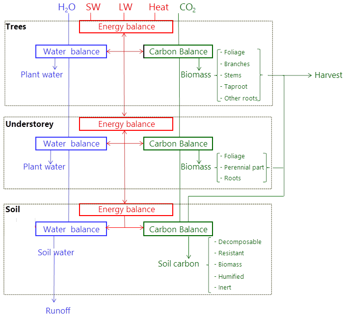
Figure 1Overview of the GO+ model. The main atmospheric fluxes exchanged with the forest are summarized as follows: H2O – precipitation; SW and LW – shortwave and longwave radiation; Heat – sensible and latent heat flux; CO2 – carbon dioxide exchange. The carbon exported as harvested material can be composed of stems, branches, foliage, stumps and coarse roots. The carbon flow from tree and understorey into the soil includes litter from foliage, branches and roots as well as harvest residue and dead parts of the understorey.
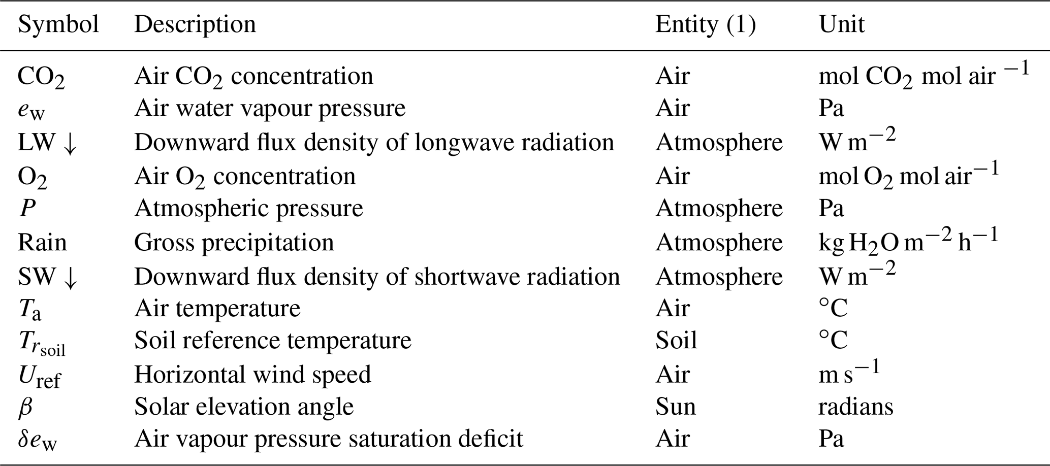
Table 1List of the forcing meteorological variables driving the GO+ v3.0 model.
The model calculations start from solving the aerodynamic and radiation transfers, energy balance, and water cycle and end with the resolution of carbon processes, plant growth and mortality. It includes several feedback processes (not shown in Fig. 1 for clarity) namely the effects of soil water and carbon content on vegetation layers, the canopy feedback of the atmospheric exchanges of radiation, and wind speed. The competition for light resource between the tree and understorey layers is explicit, whereas the two entities are treated equally for access to the soil water resource. For allowing GO+ to be run over large spatial and temporal domains with sufficient resolution, the 3.0 version of GO+ used two main simplifying assumptions releasing model calculations from time-consuming iterative computations as follows. First, the feedbacks of canopy sources on the air temperature, humidity and CO2 concentration are neglected, implying that the profile of scalar concentration gradients within the canopy are not accounted for. Second, some simple analytical solutions of the radiation transfer and energy balance calculations are used instead of iterative calculations, which implies a limited number of approximations detailed in the description section.
2.2 Radiation transfer
Each vegetation layer is treated as an isothermal turbid medium where intercepting elements, the foliage and aboveground woody parts are distributed uniformly or clumped. The calculation is operated for each layer from the top to the bottom layer. The transfer of direct and diffuse shortwave radiation, SW, and longwave radiation, LW, through each layer is calculated using the Beer–Lambert law of light attenuation with a second-order scattering. In the shortwave domain, the GO+ model follows the approach described by de Pury and Farquhar (1997), with a few adaptations described below.
2.2.1 Foliage
For both the trees and understorey, GO+ allows a dynamic partitioning between sun and shade components (Eq. S1 in the Supplement). The canopy reflection coefficients for diffuse and direct beam irradiance are calculated from (i) the leaf optical characteristics (reflectance, transmittance and absorbance); (ii) the diffuse and direct canopy extinction coefficients, kd,c and kb,c; and (iii), for the latter, solar elevation (Eqs. S2–S4). The extinction coefficients and , where the primes indicate scattered radiation, are then used to determine the fractions of light absorbed and scattered by the sunlit and shaded parts of the foliage, thus accounting for the second-order scattering of shortwave radiation. The shortwave radiation absorbed by the sunlit and shaded fractions of the trees and understorey layers is given by the sum of direct, diffuse and scattered-beam components (Eqs. S5–S7). The absorption of the longwave radiation intercepted is also simulated using the isothermal turbid medium analogy and Beer–Lambert law as detailed in Eqs. (S8)–(S9).
2.2.2 Woody parts of the tree canopy
The same formalism used for the foliage is used for modelling the passage of both shortwave and longwave radiation through non-leafy parts of the canopy, i.e. the tree branches and stems. The tree canopy leaf area index, LAIT, is substituted by the wood area index, WAIT, the latter being calculated from the aboveground biomass, mean canopy height, stem density per hectare, mean stem diameter and a trunk shape factor (Eq. S10).
2.3 Energy balance
The exchanges of longwave radiation between soil, canopy and the atmosphere are calculated according to the analytical solution proposed by Jones (1992) with minor adaptations as follows. First, for each layer c, the net isothermal radiation, Rni,c is calculated from the SW and LW radiative balance, assuming that leaf and air temperature are equal.
where KLWc, the emission coefficient for thermal radiation, is calculated following the model by Berbigier and Bonnefond (1995) completed with a term for thermal radiation from the leafless parts of the canopy (stem and branches) as
where kLW1,c and kLW2,c are extinction coefficients of foliage and is the extinction coefficient of woody parts for diffuse radiation.
The longwave radiation and heat transfer are calculated using a resistance analogue scheme with a combined resistance to heat transfer, rHR,c, that is calculated from the resistances to convective and radiative transfer, rH,c and rR,c, respectively:
Last, the temperature of each vegetation layer and air, , is derived by combining radiative and convective transfers:
Longwave emission and net radiation absorbed are then given by Eqs. (7)–(8):
The changes in the storage of heat in the aboveground biomass and air and water vapour within the canopy are neglected. The soil heat flux, G, is
where h is the thermal conductivity of soil between the reference depth (the lower limit of the soil) and the top layer of soil in contact with the atmosphere, is the soil surface temperature, and is the temperature at the lower soil limit taken as the mean annual temperature of the site.
2.4 Momentum and heat transfer
The fluxes of sensible and latent heat from each vegetation layer and the soil into the atmosphere at the reference level z are formalized as a transfer through two resistances in series:
-
the aerodynamic resistance to momentum transfer under neutral conditions, (related stability parameters equal zero), rH,c (Eq. 3) is related to the tree – or understorey – height, hc, stem density, SDc, and leaf area index, LAIc, calculated according to the formulation proposed by Nakai et al. (2008):
where the wind speed at a reference height, Uref, is derived from values provided by meteorological data using a logarithmic attenuation profile. The roughness length, z0c, and displacement height, dc, are modelled as follows:
The resistance to heat transfer is taken as resistance to momentum under neutral conditions. We neglected corrections for stable and unstable conditions and extended the use of Eqs. (11)–(12) to non-neutral conditions.
-
the canopy stomatal conductance submodel is based on a hypothetical maximum conductance, gs,max, which is modified by empirical stomatal response functions which vary between zero and unity. These functions are combined in a multiplicative polynomial equation (Jarvis, 1976) to model the responses to the air CO2 concentration, air vapour pressure saturation deficit, δew, the incident shortwave radiation, SW, and the leaf water potential, ψleaf. Since the leaf water potential depends on the tree hydraulic conductivity (Eq. 21), this model accounts for the effects of plant height on stomatal conductance (Delzon et al., 2004). The stomatal response modelled is therefore independent of the photosynthesis rate and allows for putative nighttime positive values. The individual stomatal response functions used are generic, but their parameterization is species-specific. The stomatal model includes a time constant which accounts for the response time of stomata to changing climatic or leaf water potential conditions. The steady-state stomatal conductance, and its dynamic counterpart, gs,c are
with
The sensible heat flux from the vegetation layers and soil is
Since mass transport into the atmosphere is essentially turbulent, resistance and conductance for heat, momentum and mass transport will not be distinguished further in this section. The wet and dry fractions of each canopy and soil layers are calculated dynamically using Gash's canopy water balance model resolved at an hourly time step (Eqs. S11–S14, Gash, 1979). This model, which needs few parameters, estimates the interception of incident rainfall by the canopy and the depth of water retained on the canopy. The tree trunks are treated as the foliage (Table S1). Under wet canopy conditions the stomatal resistance is assumed to be zero and the flux of water vapour exchanged with the atmosphere is transferred only across the aerodynamic resistance:
where SW,c is the water stored on the surface of the canopy and is the fraction of canopy that is wet. In the case of condensation, i.e. when , the corresponding amount is added to the rainfall and transmitted to the lower layer. The canopy temperature is not differentiated between the wet and dry fractions.
The canopy stomatal resistance is added to estimate the vapour flux emitted from the dry canopy, i.e. the plant transpiration:
The soil is treated using a specific surface resistance calculations as follows:
The resulting latent heat flux, λE, is the sum of dry and wet evaporation over the vegetation layers and soil.
2.5 Water transfer
The soil is partitioned into three horizontal layers, which are defined by their respective water content and may therefore have a variable depth and thickness:
-
the top layer A is unsaturated, i.e. its water content, θA, varies between the wilting point, θWP, and maximal water-holding capacity, i.e. the field capacity, θFC;
-
the water content of the layer B, θB, is between the field capacity and saturation, , and zAB is the lower level of layer A (upper level of layer B);
-
the layer C is saturated at θSAT and zBC is the lower level of layer B (upper level of layer C).
Water is transferred from the soil surface into the three layers according to a 1-D cascading formalism through either (i) as frontal diffusion or (ii) fast gravitational transfer according to a simple bucket model. Because the water content of B and C cannot vary – only their thicknesses can vary – the layer A, if present, is first filled up until field capacity; further water input is then transferred to the layer C that is filled until it reaches the soil surface when zBC=0. In the absence of sufficient plant water uptake, deep runoff to groundwater occurs; this depends on the local topography and hydrological environment and is modelled as
where Dmax is the maximal drainage rate which will occur when the water table is at the soil surface, zmin is the depth at which drainage of the water table ceases and kw is a shape parameter describing the attenuation of drainage rate with the water table depth. In this equation, the depth is counted as a positive number.
The soil evaporation is emitted from the upper layer, that is A, B or C. Plant transpiration is taken from the soil layers above the maximal root depth according to their respective water availability, first from the saturated layer C, then, and if necessary, from the intermediate layer B and finally from the upper layer A. Hence, when soil is saturated, i.e. zBC=0 and layers A and B do not exist, the transpiration uptake lowers the level of C and creates a layer B until zBC passes beneath the root level, i.e. zBC<zroots. The transpiration is then taken from the layer B until its water content, θB, drops down to the field capacity, θB=θFC. Layer A is then created and transpiration is taken from A.
The water withdrawn by plants is transferred from the soil to the roots and from the roots up to the canopy along a series of two hydraulic resistances, the soil-to-root resistance: rsoil, and the mean root-to-foliage resistance, rxyl.
A plant bulk capacitance, CT, is added in derivation of the two-resistance pathway (Eq. S15 from Loustau et al., 1998). Having defined a global soil-to-foliage resistance, rc, as , the canopy foliage water potential is
2.6 Carbon cycle
The carbon cycle includes a suite of processes starting with the CO2 uptake from the atmosphere by photosynthesis in the foliage and continuing with the subsequent transport and metabolic processes until carbon is exported out of the ecosystem, being returned into the atmosphere by the respiration of the vegetation or soil, leached as dissolved carbon in groundwater or exported during harvest (Fig. 1). Methane fluxes, the emission of volatile organic compounds and herbivory are neglected in version 3.0 of the model.
2.6.1 Photosynthesis
The photosynthetic carbon uptake by each vegetation layer is formalized in GO+ following Farquhar et al. (1980) and de Pury and Farquhar (1997) as the minimum of the RubP (Ribulose-biPhosphate) regeneration by electron transport and its carboxylation rate by RubisCO. The effects of leaf nitrogen and phosphorus content on photosynthesis are not implemented in the version 3.0 of the GO+ model and so are not presented here. The carbon assimilation is calculated separately for shaded and sunlit fraction of the foliage, denoted by subscript s, following the same set of equations (Eqs. 22, S17–S20).
The temperature dependency of the maximal rates of carboxylation by RubisCO and electron transport, Vcmax,c and Jmax,c, are computed according to Medlyn et al. (2002) (Eqs. S22–S28). The chloroplastic concentration in CO2, cx, is estimated from the atmospheric concentration , accounting for a series of three resistances from atmosphere to chloroplast: the aerodynamic resistance (Eq. 3), stomatal resistance (Eq. 13) and leaf internal resistance, the latter being taken from Ellsworth et al. (2015) (Eq. S21). The combination of the CO2 transport equation , where the total conductance to CO2 is , with biochemical reaction rates (Eqs. S18–S20) leads to a quadratic equation which has the solution
with
and
where the electron transport rate Jc,s, is calculated according to Eq. (S19). The net photosynthesis is then integrated at canopy layer level using the shaded and sunlit area fractions of foliage LAIsun and LAIshade (Eq. S1) and foliage temperature for estimating Km, Vcmax,c, Jmax,c and Γ* (Eqs S22–S28). At the ecosystem level, the net assimilation of CO2 and the gross primary production by the canopy foliage are therefore, respectively,
Figure 2 illustrates the shape of the stomatal conductance and photosynthesis responses to the leaf water potential at a range of leaf-to-air vapour pressure deficits. The coloured areas provide the range expected for the effect of a CO2 concentration change from 410 to 820 ppmv.
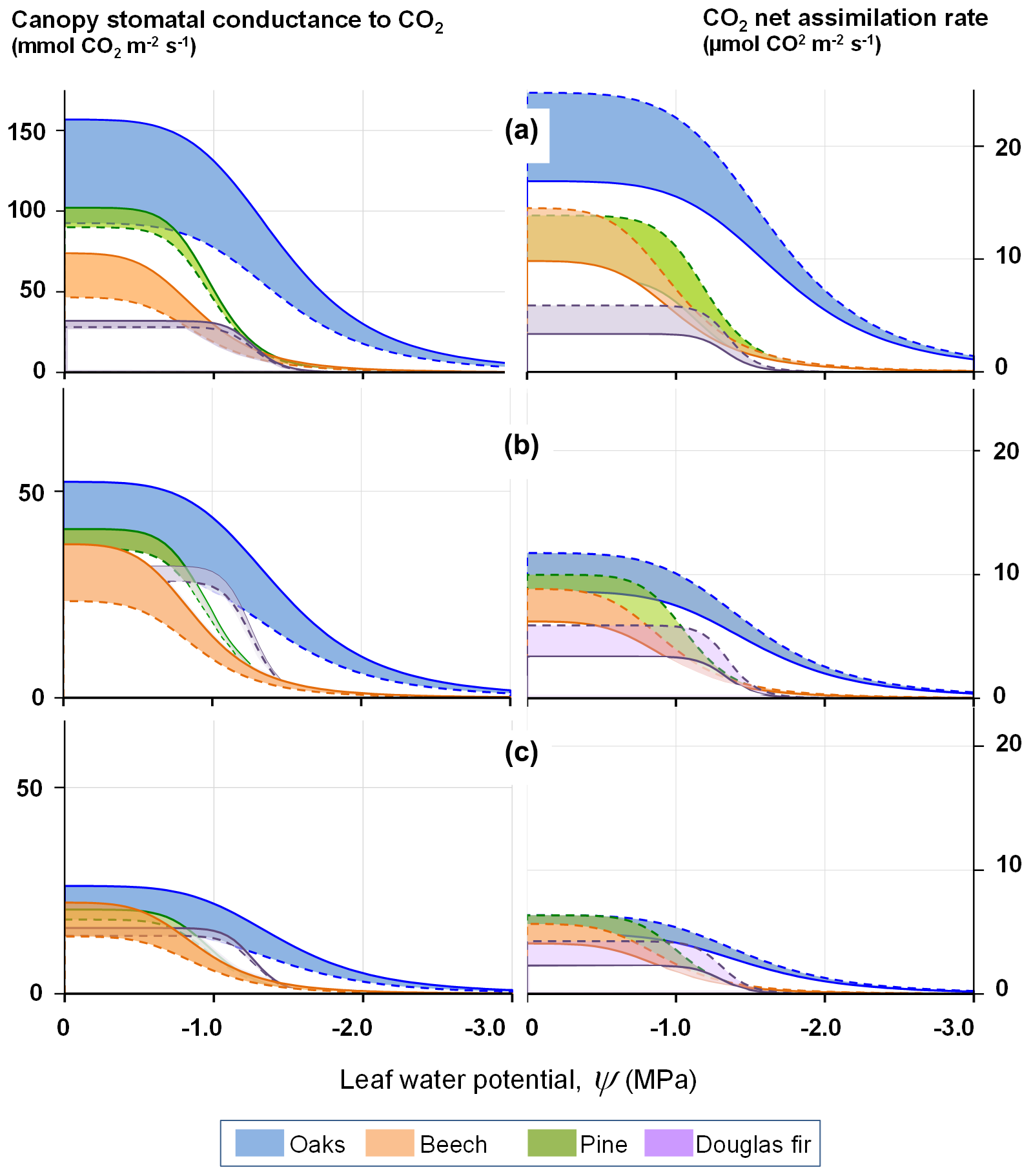
Figure 2Modelled response of the stomatal conductance (left) and light-saturated photosynthesis (right) to decreasing leaf water potential at three levels of air water vapour saturation deficit, δew: (a) 500 Pa, (b) 1500 Pa, (c) 3000 Pa, according to Eqs. (13) and (22). The response curves delineate the range of response of four tree species for atmospheric concentrations of CO2 varying between 410 (full line) and 820 ppm (dashed line).
2.6.2 Respiration
The respiration from living plants, Ra, is assessed as a mass flux of CO2 released into the atmosphere. It is partitioned between a growth component and maintenance component. The growth respiration Rg is estimated as a fixed fraction of the carbon allocated to growth that depends on the chemical composition of the organ, leaves, branches, stems and roots (Penning de Vries et al., 1974). The maintenance respiration, Rm, is a basal metabolic rate of respiration that depends on the living biomass and temperature. It is calculated separately for aboveground parts and belowground parts as follows.
-
The foliage respiration of each layer, Rmc,f is
where kTc is a temperature factor also used for the parameters representing the temperature dependency of photosynthesis (Eq. S22).
-
The maintenance respiration of other tree parts (stem, branches, taproot, coarse, small and fine roots, denoted by x) is calculated on the basis of the mass of nitrogen in living biomass, (Dufrêne et al., 2005).
where RN,T15 is the rate of maintenance respiration per unit mass of nitrogen (Ryan, 1991). The calculation of is resolved at the tree level as detailed in the Supplement Eqs. (S29)–(S33). The temperature-dependent respiration integrated over the entire tree layer, RmT, is then
where the subscript i stands for tree, SD is the number of trees per unit area and Q10,x is multiplier of maintenance respiration of organ x for a 10 ∘C temperature increase.
-
The maintenance respiration of the understorey components (foliage, roots and perennial part) depends only on their biomass and uses the same temperature response as the trees.
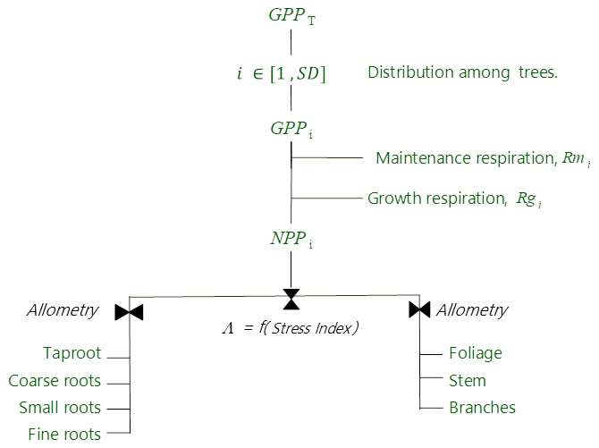
Figure 3Allocation scheme of carbon for the tree canopy in the GO+ v3.0. GPPT is the gross primary production of the whole tree layer (Eq. 23), i denotes each individual tree, SD is the number of trees per ha, Rmi and Rgi are the maintenance and growth respiration of tree i (Eqs. 25–26), NPPi is the net primary production of tree i, and Λ is a root–shoot allocation coefficient controlled by the water stress index (Eqs. 27–29).
2.6.3 Carbon allocation and growth
The GO+ allocation scheme allows a flexible allocation of carbon among trees and between aboveground and belowground tree parts. The allocation scheme of the understorey is fixed. The allocation scheme is summarized in Fig. 3. The carbon allocation between belowground and aboveground parts is regulated by a water stress index. Subsequently, the carbon is distributed among plant parts based upon empirical allometric equations.
-
For the tree stand, the growth is resolved at a daily time step for the foliage and at an annual step for the stems, branches, taproot, coarse roots, and small and fine roots. The tree growth is modelled following a three-step process.
- 1.
The carbon uptake by photosynthesis GPPT is shared among trees according to their respective contribution, λi, to the canopy foliage dry mass WL,T.
where and , SD being the number of stems per unit area. For each individual the amount of carbon allocated to growth, NPPi, is the gross primary production after the respiration of foliage, woody parts and roots have been subtracted: .
- 2.
NPPi is partitioned between aboveground and belowground parts using a root–shoot allocation coefficient Λ. This coefficient depends on the annual water stress index, Istress, that is related to the ratio of the annual tree transpiration, Edry,T, to the potential transpiration, Epot,T. The potential transpiration, Epot,T, is calculated with a stomatal model having only SW and CO2 limitations and corresponds to the transpiration of a canopy unlimited by hydrological or meteorological drought.
with
The allocation scheme allows, therefore, a shift in the annual amount of carbon allocated to growth of belowground parts, dWr,T, when the stress index increases (Landsberg and Waring, 1997). The annual net amount of carbon available for the structural growth of roots is calculated as
The corresponding amount of carbon allocated to aboveground structural parts is
The tree biomass aboveground and belowground Wa,i and Wb,i are then updated:
- 3.
GO+ allocates the amount of carbon available for aboveground growth among foliage, branches and stem and for belowground parts among taproot (stump + main pivotal root), coarse roots (diameter >20 mm), small roots (diameter between 2 and 20 mm) and fine roots (diameter <2 mm) using species-specific sets of allometric equations. Each set of values is specific to the tree species considered. Such equations link the stem diameter at breast height, D130, to the biomass of aerial parts. The D130 is substituted from the set of allometric equations so that each compartment biomass can be related to the total aboveground biomass. The foliage growth is distributed over the next growing period meaning that the current cohort of leaves relies upon the previous year's NPPT. This implies that the current year LAI depends on the previous year NPPT and stress index. The growth of the other parts of each tree is not dynamic but is calculated at a yearly resolution; it is instantaneously updated at the end of the year. The equations used for maritime pine, European beech and Douglas fir are shown as examples in Eqs. (S34)–(S62). The height of each tree is also derived from allometric equations.
- 1.
-
The understorey allocation scheme is resolved dynamically at a daily time step using two ordinary differential equations. We assume the horizontal distribution of the understorey vegetation is uniform and no individual plants are defined. The vegetation includes three compartments, the foliage, f, roots, r, and perennial parts, p. The understorey growth comprises two processes, growth and mortality, that are applied to each compartment (foliage, roots and perennial parts) with specific parameter values. The growth of understorey biomass parts is resolved at a daily time step as the minimum of a demand and a supply function, dWd,j and dWs,j, respectively.
- i.
The demand function of each compartment (foliage, roots and perennial parts), dWd,j, is the derivative of the sigmoid function, sj, times the asymptotic value of biomass, Wmax,j:
where dWd,j is the daily potential biomass increment of compartment j and , where GD is the maximal growth duration, ks a flattening coefficient (kurtosis) and the day of year by which half of the growth has been achieved, BBj being the day when growth starts.
- ii.
The supply function of compartment j, Ws,j, is the pool of carbon available for growth. It is fed by the fraction of the carbon allocated to the compartment, dWs,j calculated as
where λj is an allocation coefficient to compartment j and Rgj the respiration cost associated with the compartment j. The NPPU allocation among the three compartments is fixed by three parameters, λj, subscript j standing for f, p or r. The growth starts at the “bud burst day”, BBj, according to a simple model of accumulated “degree days” and is paused when the soil moisture deficit or air temperature drop below a fixed threshold value of SMDGU or TGU, respectively.
- i.
2.7 Vegetation phenology
2.7.1 Leaf unfolding, senescence and growth
A specific phenological model of leaf development can be specified for any tree species comprising the overstorey layer. This is illustrated for three phenological model types in the Supplement (Table S3). They include (i) a simple thermal time model (maritime pine), (ii) a parallel model combining simultaneously chilling and forcing temperatures (Douglas fir), and (iii) an alternating model assuming a negative exponential relationship between the sum of forcing units required for completing the quiescent phase and the sum of chilling units received (European beech). A single model is implemented to describe the phenology of the understorey vegetation. It includes a simple thermal time model for leaf unfolding with parameters that are identical for the three compartments: foliage, perennial part and roots (Table S5). The temperature used for accumulating degree days is the air temperature for aboveground parts and the soil temperature at 0.1 m depth for the roots.
2.7.2 Senescence
The senescence of the different tree and understorey parts is modelled according to the organ-specific turnover time and to the mortality induced by low temperature, soil moisture deficit or date, respectively (Tables S4–S5). The timing of senescence is fixed for the cohort of coniferous needles. For broadleaf species it is a linear function of the sum of the mean daily shortwave radiation( , in W m−2) accumulated from the date of bud burst until DOY=258 for European beech (Table S4), as fitted on data provided by the French ICP forest network (http://icp-forests.net/, last access: 10 June 2015) from 14 beech stands where meteorological data were recorded (Lebourgeois, 2008). This accumulated radiation model explains 60 % of the variance of the leaf senescence date across the dataset explored; it compares well with other modelling attempts requiring more parameters and variables (Delpierre et al., 2009). The understorey senescence is triggered by low temperature, soil moisture deficit or date: beyond a fixed threshold, the understorey mortality is set at a fixed rate (Tables S1, S5). The separation of dead parts from the mother plant occurs as a single event either annually at the end of the year for tree branches and roots or daily for the tree and understorey foliage. After separation, dead parts are immediately incorporated into the soil.
2.7.3 Mortality
Apart from the management operations (spacing, thinning, clear-cutting), the process of mortality of forest trees is diverse, complex, and poorly understood and documented: it is therefore not mechanistically modelled in version 3.0 of GO+. Instead, at the end of each year, the carbon balance of each tree – the difference between its annual carbon assimilation, GPPi, and its annual respiration, Rmi+Rgi – is calculated. A “natural” tree death occurs when the carbon balance of a tree is negative; i.e. the net amount of carbon allocated for growth is negative. This is mainly provoked by combinations of strong soil water deficit, air water vapour deficit and high temperatures.
The understorey cannot “die” naturally but is maintained as a perennial carbon pool that can be regarded as a survival form (seeds, rhizomes, bulbs, etc.). This allows regrowth of ground vegetation after clear-cutting. Following natural mortality, thinning or clear-cutting, the parts of harvested trees and understorey that are not exported are added to the soil pool. In particular, the part of the ground vegetation composing the understorey that is destroyed by forest operations such as soil preparation and possible discing prior to tree spacing or thinning interventions is added to the soil.
2.7.4 Tree regeneration
As with mortality, tree reproduction and regeneration is not mechanistically depicted in GO+. Instead, following the clear-cut of a tree stand, the stocking density of the next cohort of trees and the size distribution of young seedlings – or saplings – are specified. The stocking density may vary from a few hundred per hectare in coniferous tree plantations up to tens of thousands per hectare in broadleaf standards with natural regeneration.
2.8 Soil carbon
The Roth-C v 6.3 model is implemented in GO+ with only a few modifications (Coleman and Jenkinson, 1996). Only one soil layer is considered for soil carbon and the entire organic carbon stock of the soil is assumed to be included between the soil surface and the soil depth down a vertical profile modelled as exponentially decreasing with depth (Arrouays and Pelissier, 1994). The inputs of organic matter to the soil are incorporated at the time of death – or harvest – when plants die or at the time of separation from the mother plant for the senescing parts of foliage, branches, stems and roots. Mineralization and decomposition processes are discretized at an hourly time step and forced by the soil temperature at the average depth where the respiration occurs, TS,Rh, and soil moisture in layer A. The temperature at the average soil depth where the heterotrophic respiration occurs, TS,Rh, is estimated using an empirical force–restore model depending on air and soil reference temperature as follows:
The main adaptation introduced concerns the impact of forest operations on mineralization and decomposition rates as described in the next section.
2.9 Management: forest operations and harvesting, nutrient balances, wood products
The management module of GO+ is separated from the core biophysical and biogeochemical modules. Management intervenes during the model execution as a suite of operations affecting processes involved in the soil carbon dynamics or affecting the understorey layer and tree stand. The forest management schemes are described as itineraries starting from regeneration and running until the next clear-cut, thus covering the entire life cycle of the tree stand. Throughout the life of a stand, tree density is thus controlled by regeneration, climatic mortality, and thinning and cutting. Two main management strategies are implemented in the GO+ 3.0 version: coppicing and regular stand. So far the former has been used only for eucalyptus, whereas regular stand management is the main strategy used for pine, beech and oak species.The GO+ model may thus simulate the main management schemes used in monospecific even-aged forests, from short-rotation eucalyptus coppices to stands of coniferous or broadleaved species, unmanaged old-growth forests (self-thinning), and agroforestry systems (coffee plantations). The model results can therefore be used for analysing the interactive effects of management and climate change on forest energy, water and carbon balances as well as commercial production. Further developments that will account for tree species mixture and irregular forests are ongoing but not yet implemented in version 3.0.
2.9.1 Soil preparation
Although Roth-C was initially calibrated for arable soils subject to periodic ploughing, it may underestimate the abrupt effect of ploughing on forest soils (Balesdent et al., 1998; Gottschalk et al., 2010). In managed forests, soil preparation may include techniques such as tillage, moulding and discing, which may occur at only decade-long time intervals and therefore induce some drastic changes in the structure and microclimate of the upper soil horizons and organic layers. This may explain the effects of the preparation of forest soils on mineralization (Wang et al., 2018) and decomposition of the soil organic matter (Chen et al., 2004). In the GO+ model, we introduced a ploughing effect specifically for forest soils. With this scheme the effects on the soil carbon of the preparation techniques such as ploughing, moulding and discing can be prescribed in the management module at any specific time during the rotation, e.g. after clear-cut, before every specified spacing, thinning and clear-cutting operation or before regeneration. Immediately after any operation affecting the soil, the mineralization and decomposition rates of the soil carbon fraction affected are enhanced; this enhancement then decreases exponentially with time. Figure 4 shows the dataset taken from Jolivet (2000) which is used for calibrating the enhancement factor and its half-life. Table S1 provides the default values of the parameters. This approach is simple but easier to implement at multiple sites and spatial scales than the more mechanistic Gottschalk et al. (2010), which differentiates the ploughing effect according to the carbon pools described in Roth-C and to their linkage with the mineral fraction.
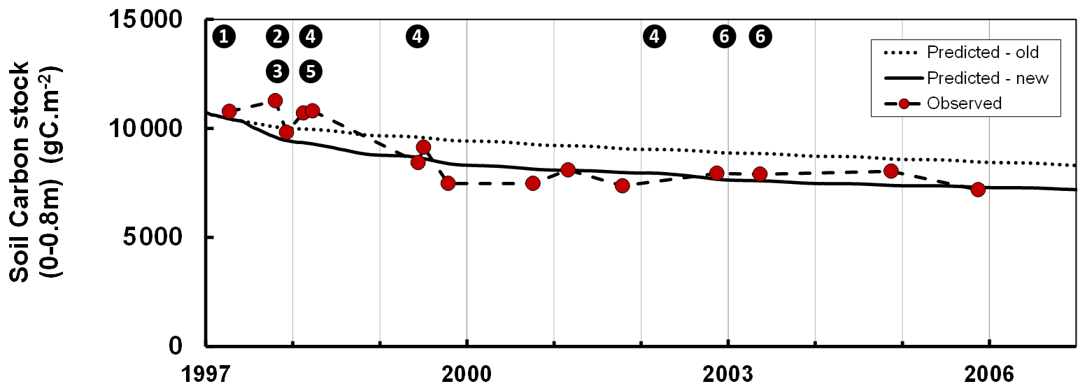
Figure 4Changes in the soil organic carbon stock during the regeneration phase following a clear-cut of a maritime pine stand as simulated by the GO+ model with and without adaptation for soil preparation (full and dotted lines, respectively) and measured in the field (grey dots). Data taken from Jolivet (2000). The numbers inset in black dots refer to the forest operation. 1: clear-cutting and logging; 2: heavy discing; 3: stump removal; 4: cover crop; 5: tillage; 6: vegetation crushing.
We also evaluated the model on soil carbon data collected by Arrouays and Pelissier (1994). Those data provide a time series of soil carbon stocks following deforestation and continuous maize cropping in Les Landes forest in southwest France. The difference between the original version of Roth-C and the GO+ version is substantial, i.e. 5 % to 12 % of the total modelled soil carbon; this difference is maintained over time. The simulation output from the improved GO+ version is closer to the observations for both the short-term changes observed during soil preparation (stump removal, slash burial, vegetation crushing) (Fig. 4) and long-term soil carbon chronosequence following deforestation (data not shown; Arrouays and Pelissier, 1994).
2.9.2 Tree stand management
The tree stand management has a dramatic impact on forest ecosystems and their functioning. The model GO+ describes mechanistically the effects of the main management alternatives applied to even-aged monospecific forest stands that dominate European forests. To this end a large framework of forest operations is implemented in the model and can be assembled to construct different technical itineraries. The operations prescribed in a given itinerary are triggered according to forest management rules as follows.
-
The stand regeneration can result from natural processes, sowing or planting, the number of seedlings and their age and size distribution being flexible.
-
The tree harvests are defined by the number and size of trees felled at each thinning and the final clear-cut. Successive spacings, coppicing, thinning and final clear-cutting occur at given stand ages or can be triggered by a competition index (Le Moguedec and Dhôte, 2012; Bellassen et al., 2010, 2011; Guillemot et al., 2014) or by target values of stand variables commonly used in forestry such as the mean tree diameter and height, stand basal area, or mean diameter and height of the 100 biggest trees per hectare at a given age. The selection of trees to be felled is flexible and can be random, from the top, i.e. the bigger trees, or from below. A wide range of thinning strategies of varying complexity can thus be simulated by the model from the relative density index used for broadleaved species to the application of the natural self-thinning rule (Reineke, 1933).
-
Specifying which tree parts are to be harvested may be any combination of stem wood, branches, foliage, stumps and roots. The harvest residues are input into the soil. GO+ predicts the size distribution of the stems harvested, thus allowing raw wood products to be routed into life cycle models, such as the C.A.T. model (Pichancourt et al., 2018), at large spatial scales.
-
Coppicing is modelled as a clear-cut followed by the resprouting of a variable number of stems, which grow from the stumps left behind. The growth of the new stems is fed by a carbon pool that corresponds to the basal part of the stem having a diameter of 1.2×D130 and a variable height (default value is 0.1 m) that is assumed to be residue. At this stage, the allocation of net primary productivity (NPP) to the aboveground part is increased until the root∕shoot ratio is restored to its equilibrium value (kλ1, Eq. 29). This allows the stand LAI to increase rapidly after cutting, as is observed for coppices.
Figure 5 illustrates the impacts on the biomass and soil carbon stocks of typical management cycles implemented in GO+ and applied commonly in European forestry. The coniferous and broadleaf standards are managed according to “Long”, “Short” and “Standard” rotations. The eucalyptus coppice includes one (Long) or two (Short and Standard) cuttings between each plantation, the Short option having a smaller diameter threshold for cutting than the Standard option. The levelling off of the beech biomass with stand age in the long and to a lesser extent in the standard options is mainly provoked by a decline in NPP due to increased biomass respiration but also by a decrease in gross primary productivity (GPP). The predicted levelling-off of production is less marked or absent for other species and management options because the thinning regime prevents the tree stand biomass to saturate. Apart from the beech stand that was simulated on a bare soil, the soil carbon dynamics are mainly marked by the periodic massive input of resistant plant material leftover following harvest operations. The soil carbon dynamics contrast sharply with the forest management options for the eucalyptus coppice and much less for the other species.
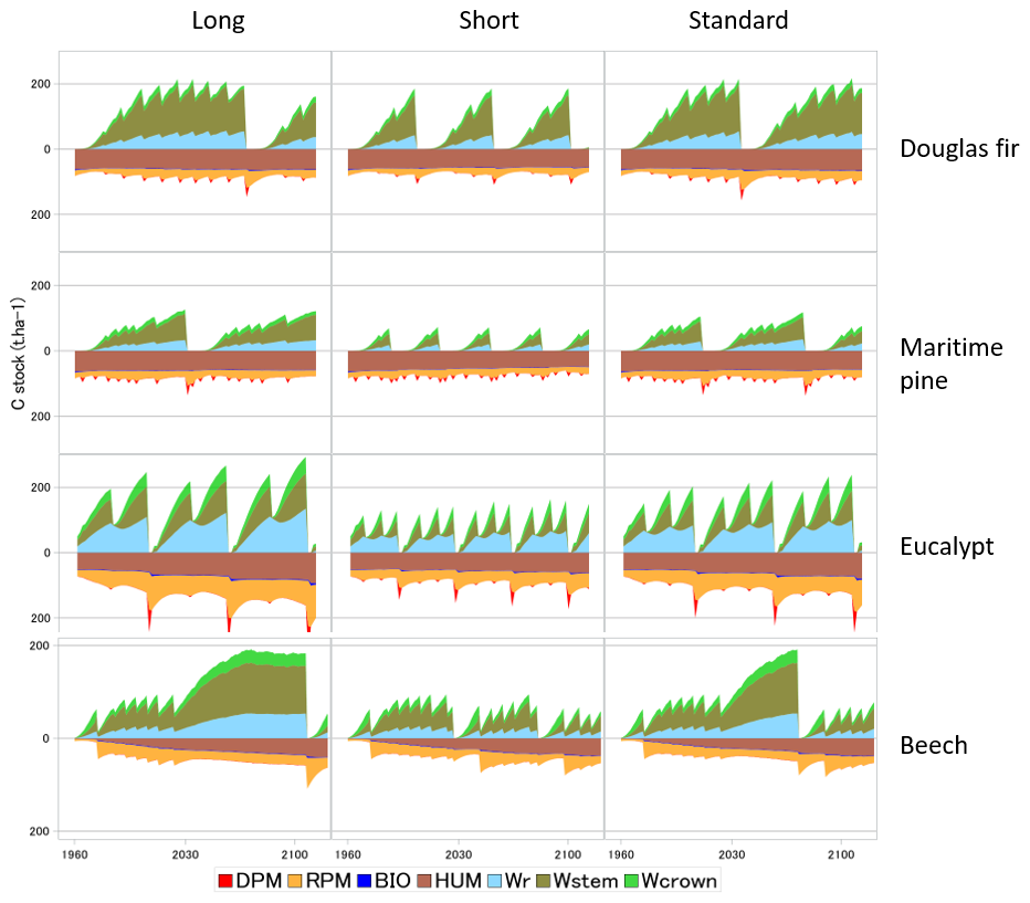
Figure 5Biomass and soil carbon stocks simulated for four species and three management alternatives. The simulations were forced by the RCP 2.6 climate scenario. The grid point location is close to the centre of the French geographical distribution of each species. The pine and Douglas fir are grown in plantations managed with thinning rules and a final clear-cut based upon the mean stem diameter. Harvested parts are the stem only (Long) or crown and stem (Short and Standard). The eucalyptus is managed as a coppice with two cuttings of sprouts before new planting. The stump age is used to trigger coppicing and final cut. The beech stand is managed according to the relative density index (Le Moguedec and Dhôte, 2012). In the examples shown, the beech stand simulated was regenerated on a bare soil with low organic matter content and no understorey. In the legend, DPM, RPM, HUM and BIO are soil carbon pools of the decomposable, resistant, humified and biological parts, respectively. Wr, Wstem and Wcrown stand for the root, stem and branch + foliage carbon pools, respectively. The soil fractions “BIO” and “DPM” have low values that are barely visible.
An application of the model at the country level is illustrated by Fig. 6 where two afforestation scenarios, the Short and Standard alternatives, were run from 2006 to 2100 in dynamic mode under RCP 4.5, starting from cultivated soils with low organic content. The short rotation is cut at 25 years and includes deep ploughing and fertilization; the Standard rotation is cut at 50 years and includes partial tillage. The simulation covers the whole French metropolitan area at an 8×8 km2 resolution (9600 pixels) and is shown only as an illustration, all simulated pixels being afforested simultaneously.
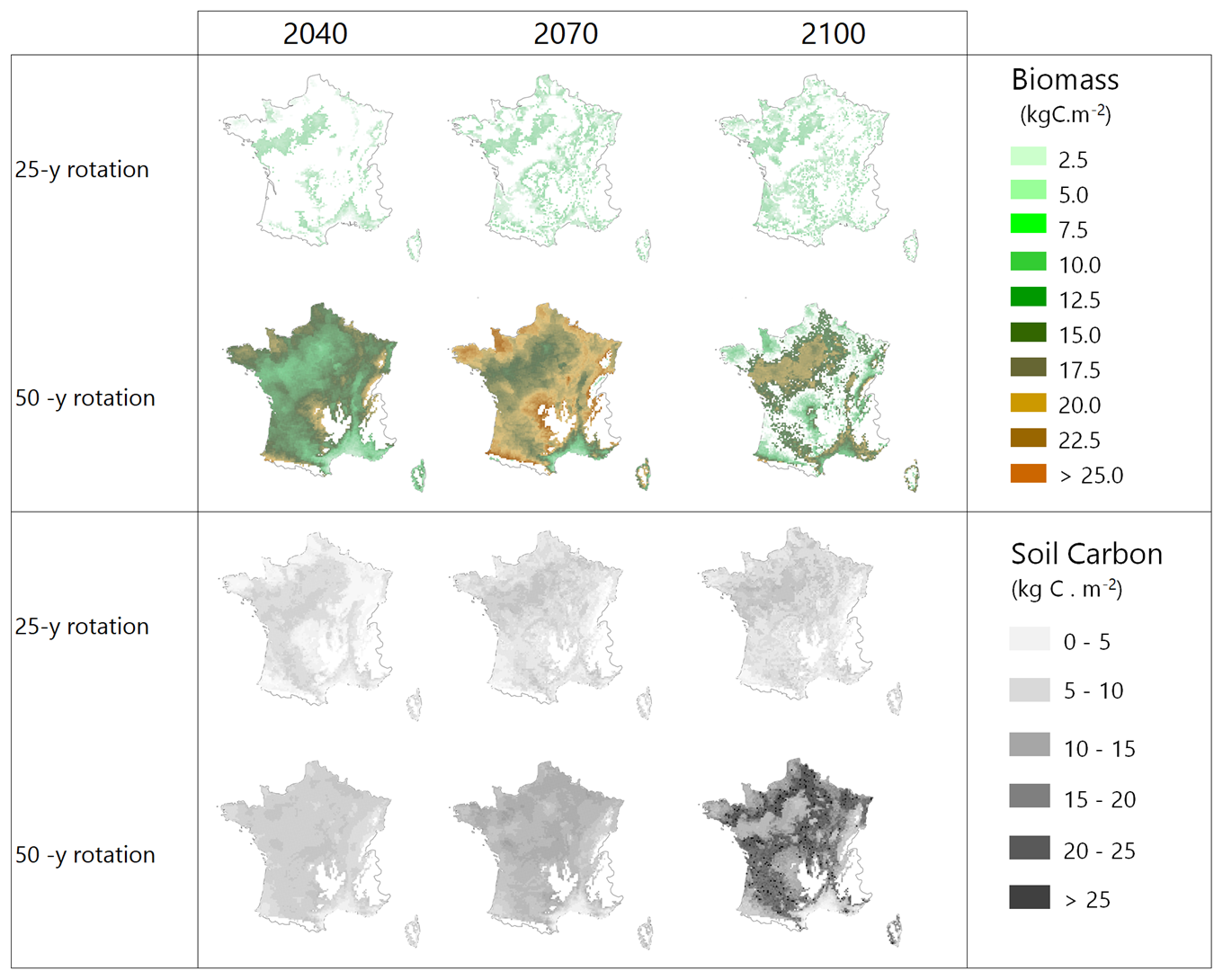
Figure 6Biomass and soil carbon stocks of maritime pine stands simulated over the entire French metropolitan area for two management alternatives under climate scenario RCP 4.5. GO+ was run dynamically from 2006 to 2100 and initialized on bare soils with new stands in 2006, mimicking the afforestation of cultivated soils.
2.9.3 Vegetation control
The vegetation management operations are described in terms of area affected and fraction of the understorey vegetation biomass destroyed. For releasing the trees from vegetation competition for light, water and nutrients or during soil preparation, a variable fraction of ground vegetation is affected and the corresponding fractions of the aboveground and belowground understorey biomass are assumed to be destroyed and added to the soil carbon pool (Subedi et al., 2014). Prior to spacing, thinning or clear-cutting, a variable fraction of understorey biomass is also prescribed to be destroyed. For instance, in the pine forests of southwest Europe, rolling heavy disc trails is a common practice at plantation and before each thinning or clear-cutting. These discing operations are applied between rows of trees on three-quarters of the soil surface area and typically affect 15 % of the soil carbon. The model simulates this practice in the following way:
-
mortality of 75 % of the aboveground biomass (foliage and perennial parts) and 50 % of the belowground biomass (roots) of understorey vegetation;
-
as described previously in Sect. 2.9.1, a 3-fold increase in the mineralization, decomposition and conversion-into-CO2 parameters of the Roth-C model for 15 % of the soil carbon with a half-life of 92 d.
2.9.4 Nutrient export
Achat et al. (2018) provide a detailed description of the nutrient module that was recently added to the core GO+ model in order to quantify the export of nutrients from the ecosystem through harvesting and soil preparation. This module evaluates the nutrient (N, P, K, Ca and Mg) stocks in standing tree biomass and soil. The nutrient outputs from these stocks through biomass harvesting can then be calculated. In short, this module calculates the main nutrient content of the soil, tree and understorey parts from the literature values and combines them with predicted values of biomass and soil components. This calculation is based on allometric equations which account for the age and size of each tree part allowing the nutrient content of trees to vary with age and size. Realistic estimates of the nutrient exports related to forest practices can thus be produced under a range of climate–management combinations, as is illustrated by Achat et al. (2018). In their simulation, the harvested tree parts were allocated to size categories, allowing them to predict the nutrient balance of management schemes according to the harvest intensity.
3.1 Testing conservation principles
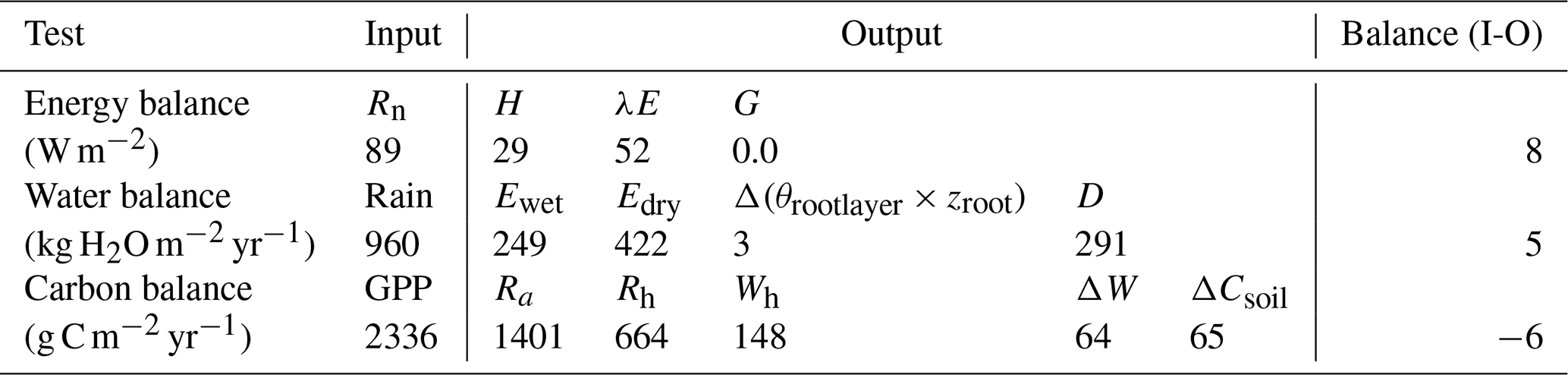
The verification tests consisted of checking the conservation of energy and mass of carbon and water for a long time series of model simulation. The period covered a typical forest stand rotation from the seedling stage to the final clear-cut; thinning and the impact of extreme natural events were included. We selected the Le Bray site to provide the benchmark data for the sensitivity analysis and evaluation of the model. The tree stand demography at this site was monitored from 1987 to 2008, with measurements of sensible heat, CO2 and H2O fluxes and meteorological variables starting in 1996. The period starts in 1984 and ends in 2010. It includes a series of dry years (1989–1991, 2002–2003, 2005–2007) and the December 1999 “Klaus” storm that felled or broke 22 % of the trees. The model was run from 1984 to 2001 forced with meteorological data measured at the French synoptic network station being interpolated across the 8×8 km2 SAFRAN grid. The number and size of the trees thinned and felled for this period in 1991, 1996, 2001 and 2005 were also used to prescribe the thinned and wind-thrown trees. The verification test results are summarized in Table 2.
-
The average hourly gap in the energy balance was 8 W m−2, that is 9 %. This gap results from the extension of neutral regime to stable and unstable conditions which results primarily in a slight underestimation of the convective heat fluxes LE and H. Nakai's model for estimating roughness length and displacement height leads to underestimate H for a low value of leaf area index that is below 1.5 m−2 m−2.
-
For the water balance, we checked independently that the annual amount of precipitation from 1984 to 2010, rain, was correctly allocated among interception by the canopy and soil layers, Ewet, vegetation transpiration, Edry, groundwater discharge or runoff, D, and the variation in the soil water stock over this period, Δ(θrootlayer×zroot). The discrepancy found was 5 mm yr−1 over a total amount of 960 mm yr−1, that is 0.5 %.
-
The closure of the carbon balance was also satisfactory, the balance between the gross primary production and the sum of carbon stock changes in biomass and soil, and harvested carbon plus the ecosystem respiration being less than 0.3 %. The mean annual net ecosystem exchange (NEE) over the period was 266 g C m−2 and is partitioned among three parts: the amount of carbon exported by harvesting, Wh, and the net annual increments in biomass, ΔW, and soil organic carbon, ΔCsoil.
Table 2Verification tests operated on the model. The test is a simple conservation test applied to the annual values of energy, water and carbon fluxes over the 1984 to 2010 period.
3.2 Parameterization
The complete list of the parameters of the model is provided in Table S1 together with appropriate references. Most of the main parameters of the model have direct observational counterparts and their values were extracted from the literature or open data sources.
3.2.1 Soil
The soil parameters of the GO+ model – as listed in Table S1 – are essentially functional and not descriptive. The rooting depth, zroots, is the depth equivalent of the soil volume affected by the root water uptake. It should not be interpreted as the maximal depth at which roots can be observed – that can be substantially deeper. The parameters θFC, θSAT and θWP have been estimated by pedotransfer functions from the kinetics of soil humidity retention curves collected over Europe and France (Wösten et al., 1999; Dobarco et al., 2019). The parameters are dynamic and depend upon the organic matter content of the soil calculated at a daily resolution. The soil water potential ψsoil (MPa) and hydraulic resistance rsoil (Eq. 19) are calculated from the soil texture and water content following Van Genuchten (1980) with soil texture-dependent parameters estimated using the approach developed in Ghanbarian-Alavijeh et al. (2010).
Initialization of the soil carbon stock is prescribed by the user and may correspond either to observed values or to steady-state values simulated by model spin-up. The organic layers aboveground, eventually including coarse woody debris, are conceptually included in the decomposable and resistant plant material fractions of the soil organic carbon, DPM and RPM, respectively. They are not separated from the mineral soil (layers ) for the calculations of energy and water exchange. Each type of plant material (foliage, branches, stem, roots, perennial part of the understorey, etc.) is characterized by a specific prescribed composition of decomposable and resistant plant material for each species considered.
3.2.2 Vegetation layers
The model parameters generally refer to the entire vegetation layer, i.e. to the tree foliage, tree stems, understorey or soil layers. This is certainly the case for carbon metabolism parameters related to the vegetation respiration or photosynthesis. The main model assumption concerns the horizontal homogeneity of vegetation layers and implies within-population variations in canopy parameters are ignored. Ideally, the optical and radiative parameters of the canopy layers will have been estimated from data observed either at leaf or canopy levels, in situ or remotely (Hassika et al., 1997; Breda 2003). The stomatal conductance model is parameterized from measurements upscaled to the canopy level (Granier and Loustau, 1994; Granier et al., 2000b; Rayment et al., 2000, 2002). The response functions have been thus parameterized based upon the data available from Granier and Loustau (1994), Granier and Breda (1996), Delzon and Loustau (2005), and Granier et al. (2000b) for pine, oaks and beech, respectively, or Van Wijk et al. (2000) for Douglas fir, and Medlyn et al. (2001) for the CO2 response.
The bulk root-to-leaf tree hydraulic resistance is modelled empirically from literature data documenting combined measurements of transpiration or sap flow and soil and leaf water potential (e.g. Loustau et al., 1998, 1996; Delzon et al., 2005; Granier et al., 2000b). The parameters used for describing the rainfall interception and its retention by the canopy layers were extracted from field data analysis (see discussion on parameters estimates in Muzylo et al., 2009). In version 3.0 of the model, the value of the fraction of carbon allocated to growth is identical for all biomass parts and fixed at 0.28 (Penning de Vries, 1974).
The phenology model of understorey vegetation is based on the understorey at Le Bray and other sites (Loustau and Cochard, 1991; Moreaux, 2012).
The allometric parameters used for allocating the net carbon produced to the different tree parts are derived from sets of allometric equations published in the literature and commonly available for the main commercial tree species. Most of them are robust enough to be applied to a range of soil, climate and management conditions (e.g. Gholz, 1979; Wutzler et al., 2008; Shaiek et al., 2011). The leaf area index is calculated from the total foliage biomass using the specific leaf area as follows:
where ξ is the leaf-area-to-LAI ratio.
We focused the sensitivity analysis presented below on the Le Bray site that was monitored from 1987 to 2010. It is a well-documented site and the data meet our objective, which was to verify the consistency of the model rather than to investigate geographical or climate variations in ecosystem functioning. A one-at-a-time (OAT) sensitivity test was carried out considering first the model parameters and second the climate variables. This analysis aimed to (i) check the consistency of the model behaviour in response to step changes in its main parameters and meteorological forcing variables; (ii) investigate possible interactions between the model sensitivity and climate; and (iii) compare the short-term to the long-term sensitivities of the model.
We used the time series of meteorological data interpolated across the SAFRAN grid from 1970 (planting) to 2010 (final cut) as well as the parameters related to soil characteristics and the forest tree stand (stocking density, soil preparation, understorey removal, thinning and harvest). The data used are available at the ISI-MIP project web site and the Fluxnet database (https://doi.org/10.18140/FLX/1440163). We analysed the sensitivity at three temporal resolutions: hourly, annual and full rotation (40 years). The parameters' mean values, the meteorological and soil datasets, and initial stand conditions were all taken from the European data cluster database (http://gaia.agraria.unitus.it/home, last access: 2 July 2017). The sensitivity index of a given model variable Y to a parameter – or variable – k was calculated as its response to a step variation in k as
where kref is the reference value for the parameter. All the other parameters are fixed at a nominal value (mean or final value). This index is the variation in Y in response to a 10 % step change in k. To some extent, the Ik values are more meaningful than mean – or sigma – normalized indices, especially for variables that may take values close to zero such as NEE. The relative values were also computed to facilitate the comparison between parameters across Figs. 7–9. The relative values
were also computed to facilitate the comparison between parameters.
4.1 Sensitivity assessment: model parameters
The sensitivity analysis of model parameters was restricted to a subset of the 28 parameters with the aim of giving a general assessment of the model behaviour in response to its parameter variations. The parameters considered are distributed among six groups related to different processes or vegetation layers: structure and allometry, phenology, radiation transfer, soil parameters, tree physiological parameters, and understorey physiological parameters. They cover, therefore, the main processes accounted for by the model: leaf unfolding, growth and senescence, radiation and energy balances, hydrology, photosynthesis, respiration, soil carbon balance, tree growth, and production. The parameters are assumed to be independent; i.e. their effect on output variables is approximately additive. The effects of factor interactions on the output variance are neglected with OAT methods, which are therefore only applicable to strictly additive models (Campolongo and Saltelli, 1997). The Y output variables describe the energy balance, water and carbon cycles, carbon balance, and tree canopy growth and structure, resulting in a total of 21 variables. The sensitivities of variables related to canopy growth and structure are shown only for the entire rotation. The hour and year sensitivities were calculated separately for a wet year and a dry year, 1994 and 2005, which received precipitation of 1271 and 681 mm, respectively. For each year, the same set of parameter values and the same initial soil and stand conditions were used. Since the hour and year sensitivities provided essentially the same sensitivity profile, only the year sensitivity is shown. Figures 7–9 show the relative sensitivity index for selected parameters, whereas the complete table of results are given in Figs. S1–S3 in the Supplement.
Independent of the annual climate, the most influential groups of parameters were first the soil characteristics (the rooting depth and water contents at field capacity and at wilting point) and, second, the tree canopy physiological parameters and the specific leaf area of both tree and understorey foliage. The model parameters related to the radiation transfer, , phenology, BBT and GDU had a lesser influence. The relative sensitivity of output variables increased according to their position in the process chain, the sensitivity of end variables (e.g. NEE) being the largest and reaching 14 % and 45 % for the 1994 (wet) and 2005 (dry) year, respectively. The higher sensitivity of NEE is because its sensitivity accumulates the impacts of parameter changes on the canopy photosynthesis, GPP, and autotrophic respiration, Ra. Conversely, the energy balance and water balance components, Rn, H, λE and runoff, D, exhibited a low relative sensitivity, their relative change being close to 0.04 and exceeding 0.10 only for the soil water content at field capacity, θFC, which has enhanced the soil water storage and mitigated the water stress impact. Comparatively, the model outputs were more dramatically affected by the changes in the wilting point θWP because of its larger impact on the soil pressure head, water potential and hydraulic resistance and in turn on leaf water potential (Eq. 21), canopy stomatal conductance (Eq. 13), photosynthesis (Fig. 2), stress index and allocation (Eq. 29; see also Table S5 the impact on understorey). The sensitivity of the carbon balance components was distributed more evenly among the parameter groups. Comparing the sensitivity of the variable groups between 1994 and 2005 also revealed differences that can be related to the contrasting amount of precipitation and related impacts on soil moisture deficit and plant water stress. The absolute sensitivity was higher for the wet year 1994 because the absolute annual values of most variables were higher for this year. Apart from the respiration components Ra,RECO and Rh, the relative sensitivity of output variables almost doubled in 2005. We observed a shift in the sensitivity of the carbon balance components NEE, GPP and NPP to the photosynthetic quantum efficiency, αT, and carboxylation efficiency, Vcmax, that was prominent in 1994 (wet year) and minor in 2005 (dry year). The opposite was observed in 2005 for the soil water content at wilting point, whose sensitivity increased from 14.4 %, 3.4 % and 6.2 % in 1994 to 45.5 %, 8.6 % and 13.7 %.

Figure 7Relative sensitivity index values of the main variables related to the energy, water and carbon fluxes to model parameters for the years 1994 (wet, in blue) and 2005 (dry, in red) at the Le Bray site. The abbreviations of the variables (vertical axes) are explained in Table A1 and the parameter abbreviations (inset) are detailed in Table S1. The horizontal bars in each box gives the relative sensitivity of 10 variables listed along the y axis to the parameters named in the box. A positive value means that the output variable increased in response to an increase in the parameter value.
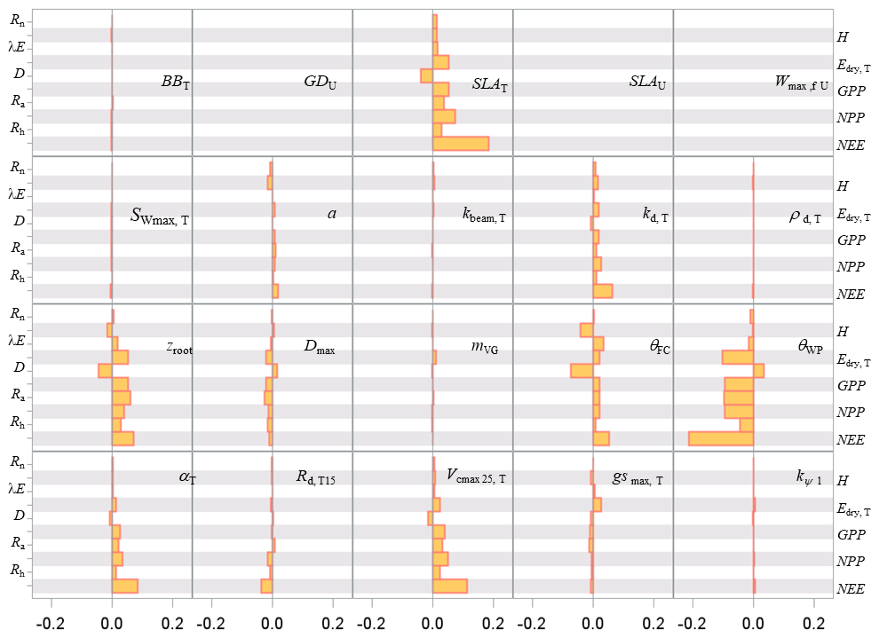
Figure 8Sensitivity index values of the main variables related to the energy, water and carbon fluxes to model parameters over a full rotation (1970–2010) at the Le Bray site. The abbreviations of the variables (vertical axes) are explained in Table A1 and parameter abbreviations (inset) are detailed in Table S1.
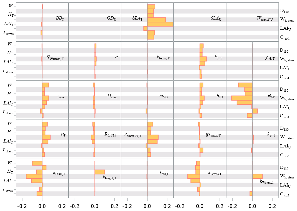
Figure 9Sensitivity index values of the main variables related to the carbon stocks in biomass and soil to model parameters over a full rotation (1970–2010) at the Le Bray site. The abbreviations of the variables (vertical axes) are explained in Table A1 and parameter abbreviations (inset) are detailed in Table S1.
The pattern of the long-term sensitivity evaluated from 1970 to 2010 is shown in Fig. 8 for the “flux” variables and Fig. 9 for the tree growth and “stock” variables. The main features previously shown on annual values were confirmed except that the impacts of the foliage area-to-mass ratio, SLA, and diffuse light attenuation coefficient kd were enhanced, whereas the understorey related parameters had less influence. The sensitivity of the biomass and soil carbon stocks (W and Csoil), mean stem diameter and height reached in 2010 (D130 and Hc), and cumulated harvestable production (Wh,stem) was consistent with the patterns observed previously on fluxes. The commercial production was the most sensitive to the model parameters SLA and θWP and to the allometric parameters , kIstress1 and kstem,1.
4.2 Sensitivity assessment: meteorological variables
The model behaviour in response to variations in meteorological variables was analysed following a similar approach. We considered the following variables: air temperature, atmospheric pressure, precipitation, mean horizontal wind speed, downward shortwave and longwave atmospheric radiation, ambient CO2 concentration and water vapour pressure saturation deficit, and the fraction of diffuse radiation. The air temperature and air vapour saturation deficit were changed by ±1 ∘C and ±200 Pa, respectively, and other variables were changed by ±10 %. The results are presented in Fig. 10 for the annual sensitivity and in the Supplement (Fig. S4) for the long-term sensitivity. The main conclusions are summarized below.
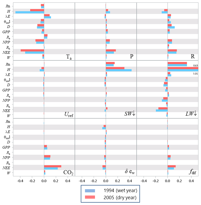
Figure 10Relative sensitivity of the main variables related to fluxes of energy, water and carbon to meteorological variables for a wet (1994) and dry year (2005) at the Le Bray site. The definition of the variables is provided in Tables 1 and A1.
The overall model behaviour was consistent with the current knowledge about canopy responses to climate for the ecosystem considered: a temperate Atlantic coniferous ecosystem growing on a well-drained sandy soil for the present case (Granier and Loustau, 1994; Medlyn et al., 2001, 2002, 2005; Davi et al., 2006; Moreaux et al., 2011, 2020). On an annual basis, the energy balance components Rn, H and λE were mainly affected by incident radiation, LW↓ and SW↓ and Tair, whereas the carbon balance variables GPP, Ra, NPP, Rh and NEE were more sensitive to CO2, fdif and precipitation rain. The negative response of the sensible heat flux H to the air temperature was essentially due to the asymmetric response of H with respect to the sign of Ts−Tair that was amplified when Ts−Tair was negative. Changes in the air temperature and water vapour saturation deficit had a negative effect on all variables except the latent heat flux and respiration for the air temperature. It is worth noting that the effects of CO2 and fdif were first to impact GPP and then to affect NPP () and lastly NEE (). The air temperature and incident longwave radiation also had significant impacts on the respiration terms Ra and Rh. The weak response of the carbon processes to a 10 % change in SW↓ has also been observed, e.g. by Delpierre et al. (2012); under temperate climate, it was not unexpected since the light is not limiting at this site. The main contrast between the 1994 and 2005 climates was observed in NEE and H, the sensitivity of the former being enhanced in 2005, while H was conversely more sensitive in 1994. The full rotation sensitivity profile of the “flux” variables (Fig. S4) was identical to the annual sensitivity profile, apart from the biomass and soil respiration, Ra and Rh, and consequently NEE. In particular, the sensitivity of Ra to the air temperature and longwave incident radiation was positive on an annual basis, as expected from Eqs. (24)–(26) but became negative over the long rotation. This reversal is induced by the long-term impacts of atmospheric and soil droughts caused by the step increase in temperature ; this is clearly shown by the enhancement of the stress index in response to the temperature (Fig. S5). The temperature step increase depleted the biomass growth, W, and in turn photosynthesis GPP and respiration Ra. The same response is shown to the longwave radiation LW↓ that increased the water stress index Istress in the long term.
4.3 Uncertainty assessment
For assessing the uncertainty of the main variables simulated by GO+, we used a simple Monte Carlo approach where 2500 sets of parameter values were randomly drawn from their distribution range. For each set, the model was run for the year 1994 at Le Bray. Based upon the previous sensitivity analysis, we retained the 14 most sensitive parameters for assessing how errors in parameter values are projected on GO+ output variables. The parameters selected were assumed to be independent. We are aware this assumption may not hold for biological and physiological parameters, but we lack quantitative relationships that would allow us to link them and define a more sound sampling design. The probability distribution assigned to each parameter was by default a normal distribution function whose standard deviation was derived from the literature or unpublished field observations or, when these were lacking, was fixed empirically (Table 3). The resulting distributions are shown in Figs. 11–12 for the ecosystem variable values.
Table 3List of the parameters used for uncertainty propagation in the GO+ model, their reference value and standard deviation.

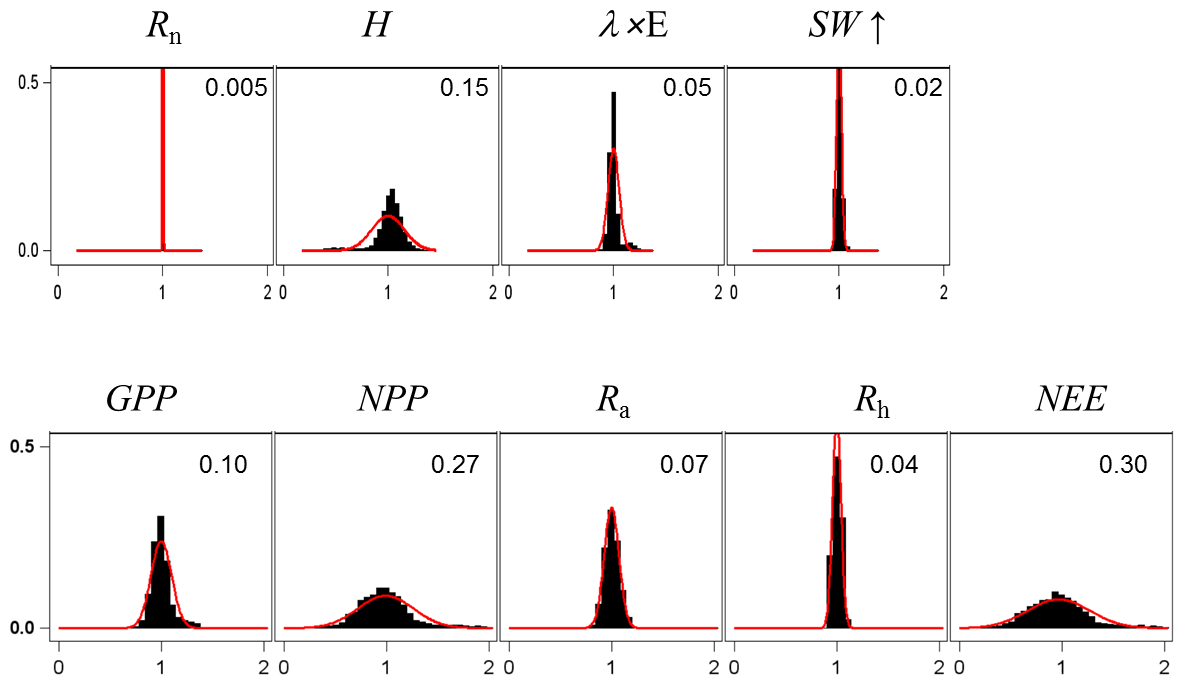
Figure 11Normalized uncertainty in the annual mean values of flux variables predicted by the GO+ model. Each graph shows the distribution of variable values generated from 14 parameter distributions (Table 3). Red curve is the normal distribution fitted and number inset is the standard deviation. The variables abbreviation are explained in Table A1.
The output variables were standardized to their mean value in order to compare the uncertainties among variables and vegetation layers. Only the ecosystem variables are shown; the uncertainty in variables referring to canopy and soil layers are reported in the Supplement (Figs. S6–S8).The uncertainty range of the energy balance components and ecosystem shortwave albedo was relatively small. It was highest for sensible heat flux, H, and lowest for the net radiation, Rn. This was attributed to the relative accuracy of the attenuation coefficients in direct and diffuse light that were both measured at this site (Berbigier and Bonnefond, 1995) and the fact that the uncertainty of the longwave emissivity was not considered. In addition, compensation effects between canopy layers and soil might have reduced the range of simulated net radiation. Compensation between layers may also explain the relative precision of the model in the ecosystem albedo because any error in the radiation transfer through the upper canopy will mechanistically induce an opposite change in the understorey balance. Indeed, the error generated in the energy balance components of the vegetation canopy was higher for the understorey and the soil; these were poorly constrained as compared to the tree and ecosystem energy balance. The uncertainty in carbon flux variables was higher than that for the energy balance, especially the NEE that accumulated the errors generated in both the GPP and the autotrophic, Ra, and heterotrophic, Rh, respiration components. Our experiment might have exaggerated the error in NEE and NPP since the values of photosynthetic and respiration parameters were drawn independently ignoring the functional link between photosynthesis and respiration. Nevertheless, this relatively large error in NEE will limit the use of its observational counterpart for evaluating the model.
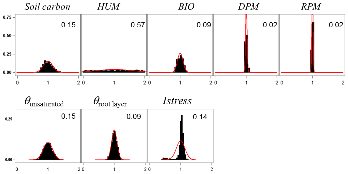
Figure 12Normalized uncertainty in the main soil variables simulated by the GO+ model. Each graph shows the distribution of variable values generated from 14 parameter distributions (Table 3). The red curve is the normal distribution fitted and the numbers inset is the standard deviation. The variable abbreviations are explained in Table A1.
The uncertainty in the annual variation in soil carbon stocks showed contrasting patterns depending on the components considered. The high accuracies in RPM and DPM were to some extent artefacts since the litter biomass was prescribed so that the only error source was caused by the mineralization and humification processes. Conversely, the HUM component showed very large uncertainty which was attributed mainly to the fact that uncertainty was related to the stock change that was very small over a year. Overall, the annual change in soil carbon stock was constrained with a standard deviation of 15 %. The same magnitude was found for the annual change in the soil water content of the unsaturated layer, whereas the annual change in the total amount of water in the rooted zone was estimated with a precision of 9 %. The annual changes in biomass and its components were not well constrained, its standard deviation exceeding 0.3 in the tree layer and 0.5 in the understorey (Fig. S8). This was not unexpected because the net biomass change is the end result of the whole chain of processes described in the model (phenology, radiation transfer, energy balance and evaporation, photosynthesis, respiration and allocation, and growth), and this chain accumulates their related errors. In addition, the assumption that the parameters are independent might have inflated the uncertainty in biomass changes.
Because GO+ encompasses full rotation duration, we were able to test the model against long time series of fluxes and stocks at both daily and annual resolution (Thum et al., 2017). To this end, two types of data were used and the model performance was assessed through two comparisons. First, is a comparison of hourly values of flux data between observed and predicted values. The second uses annual values of stand growth data. The statistics used are the root mean square error between observations and simulated values, RMSE, the variance fraction explained by the model, R2, and the systematic and random model errors which assess the bias and precision of the model, respectively (Wallach and Goffinet, 1989).
5.1 Data
The time series of daily values of energy, water and carbon dioxide fluxes, i.e. net radiation, Rn, latent heat flux, λE, and net CO2 fluxes, NEE, used in experiments (1) and (3) were obtained from tower stations and taken from the European fluxes database cluster and the Fluxnet Database (URL: http://fluxnet.fluxdata.org, last access: 14 August 2017) for Douglas fir sites. The variables used are determined from site measurements of SW↑, SW↓ and LW↑, LW↓, vertical fluctuations of wind speed, U, and fluctuations of CO2 and water vapour concentrations. The values are further processed for quality checking, filtering and gap filling. Unless mentioned, they are all level-3-type for Rn and level-4-type for λE and NEE. The level-3 data are standard files provided by stations. The level-4 data are filtered, gap-filled using the marginal distribution sampling method (Papale et al., 2006; Moffat et al., 2007) and aggregated at different time resolutions, from half-hourly to yearly. Other variables commonly used for model testing such as ecosystem GPP, RE or NPP are derived indirectly from primary measurements. They were, therefore, not used in the model evaluation because that would have introduced redundancy with the test on NEE. Table 4 presents the datasets used and their origin. Seven stations were selected because they cover a large part of the geographical range of three important European commercial tree species and also embrace a wide range of tree stand age.
The data used in experiment (2) are a set of 11 long-term records of stand growth that were mostly taken from the Profound project database (Reyer et al., 2019). The site characteristics and data sources are detailed in Table S6. In this evaluation, the model performance was assessed using the annual series of stem diameter at 1.3 m height (D130) and basal area (BA) of the tree stands. Three common commercial species are represented: maritime pine, European beech and Douglas fir at different locations across Europe and British Columbia. Various tree ages and thinning regimes are used. We compared the annual change of the stem mean diameter, ΔD130 (cm yr−1), and basal area, ΔBA (m2 ha−1 yr−1), that is the cross-sectional area of tree stems at 1.3 m height over 1 ha. The later can be taken as a proxy for the carbon storage in biomass for which no direct measurement method exists. Moreover, compared to flux values determined from turbulent variables, the stem diameter and basal area are measured with a low uncertainty (1 %–5 % error) and cover a wide range of climatic, soil and management conditions.
Table 4Characteristics of the sites selected for long-term series of daily fluxes of net radiation, latent heat and CO2.
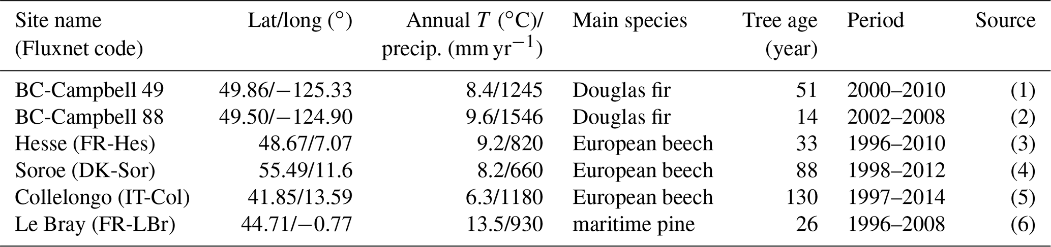
(1)–(2) Fluxnet, Humphreys et al. (2006). (3) European database, Granier et al. (2000a). (4) European database, Pilegaard et al. (2011). (5) European database, Scartazza et al. (2013). (6) European database, Berbigier et al. (2001).
Table 5Statistics of the model evaluation with daily flux values of net radiation, Rn, latent heat flux, λE, and net ecosystem exchange, NEE, at six sites: R2 and RMSE. The daily average of the observed (O) and predicted values (P) are given.
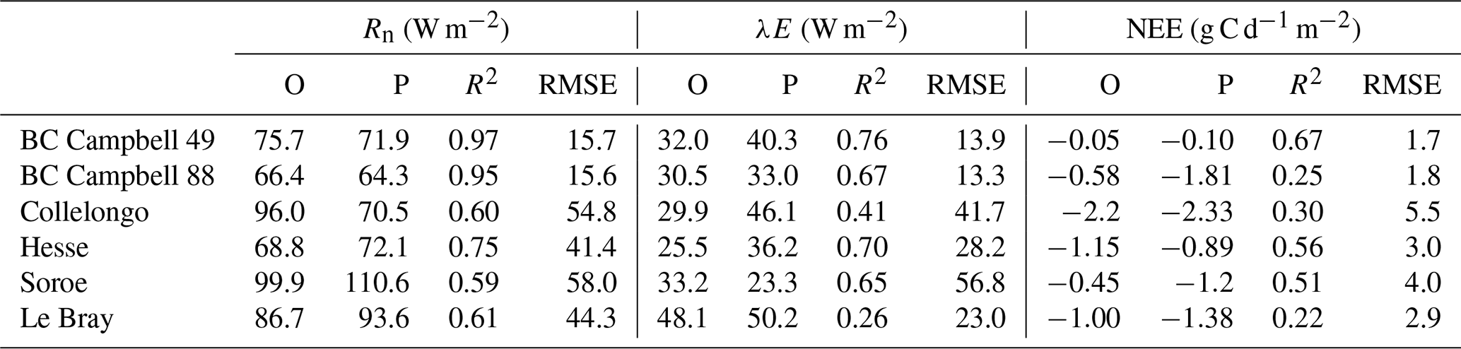
Table 6Statistics of the model evaluation with daily flux values at six sites: systematic and random errors.

s: systematic error; u: random error.
5.2 Results
To assess the overall performance of the model, we need to relate the RMSE and its systematic and random components (Table 5) to the model uncertainty in Rn, λE and NEE. The model errors were larger than the respective uncertainty of the three variables calculated in the previous section. Indeed, our uncertainty analysis used parameter values that had been obtained from local measurements – no site calibration was carried out in this comparison, i.e. a single set of parameters was applied to every species, ignoring the acclimation and plasticity of most vegetation traits (Bloomfield et al., 2018). It shows that the model itself introduces a substantial epistemic error in addition to the uncertainty linked to the parameter values. The model error was smallest for Rn and largest for H (not shown), λE and NEE. The error in H may be due to the model making the approximation that the aerodynamic resistance to heat transfer can ignore stability corrections. The NEE predictions might be affected by the simplifications made to the timing of secondary and primary growth of trees and related respiration. In addition, the model represents the source–sink activity and not the transport of water or CO2 to the reference level. Such a transfer is included in the flux values measured at ecosystem stations and adds a substantial random noise to flux values. Testing the model predictions against observed values at increasing time integrals from an hour to 365 d, we observed that the variance fraction of Rn, NEE and E explained by the model increased with the time span until the (90 d) season length and then dropped at longer time spans (Table S7).
The sources of error are multiple and it should be noted that the data themselves are subject to measurement and calculation errors currently assumed to lie within 10 %–15 % of the daily values used. The meteorological data used may also be a source of errors, i.e. at Le Bray where they were interpolated from the main French national meteorological network. Second, the fact that long time series of variables were used for this evaluation exercise makes the model results affected not only by possible errors and approximations in processes directly involved in the energy balance and carbon cycle, but also by possible faults affecting the processes describing the vegetation dynamics, i.e. phenology, carbon allocation, tree growth, mortality, forest operations or soil carbon. For this evaluation, the model was actually run from the start to the end of the decadal time series without recalibration. This is in particular the case of the Le Bray site where simulations were initiated in 1984 and run until 2000.
The evaluation of the model by comparing its output with long-term inventory records reveals that the predictions are relatively close to the observed values, both in terms of accuracy and precision (Fig. 13). Since only few data were available from inventories, in this figure we pooled together the results of the 11 sites analysed. The data observed are prone to smaller errors (typically 5 %) than the previous flux data but the information about the station characteristics and meteorological data used for modelling are more uncertain. This uncertainty is because reliable series of meteorological data, i.e. measured on-site, are not available and the information on soil characteristics can be poor. In addition and apart from the Le Bray site, we only had vague information about the criteria used to select which trees are thinned. We used the annual increment rather than the annual raw values of D130 and BA because the latter are actually cumulative variables including large temporal autocorrelation. The predicted ΔBA were close to the observed ones in general, with most values being positive but close to zero. Interestingly, the model accuracy was mainly constant along all values ranging from −7 to +5 m−2 ha−1 yr−1. The predicted ΔD130 was satisfactorily simulated by GO+. Given these uncertainties and the fact that no site-specific calibration of parameters was used, the evaluation test shows that the model departs only slightly from measurements on average, with relatively small biases. Its performance was similar across sites despite the range of species, age, management and location covered by the dataset.
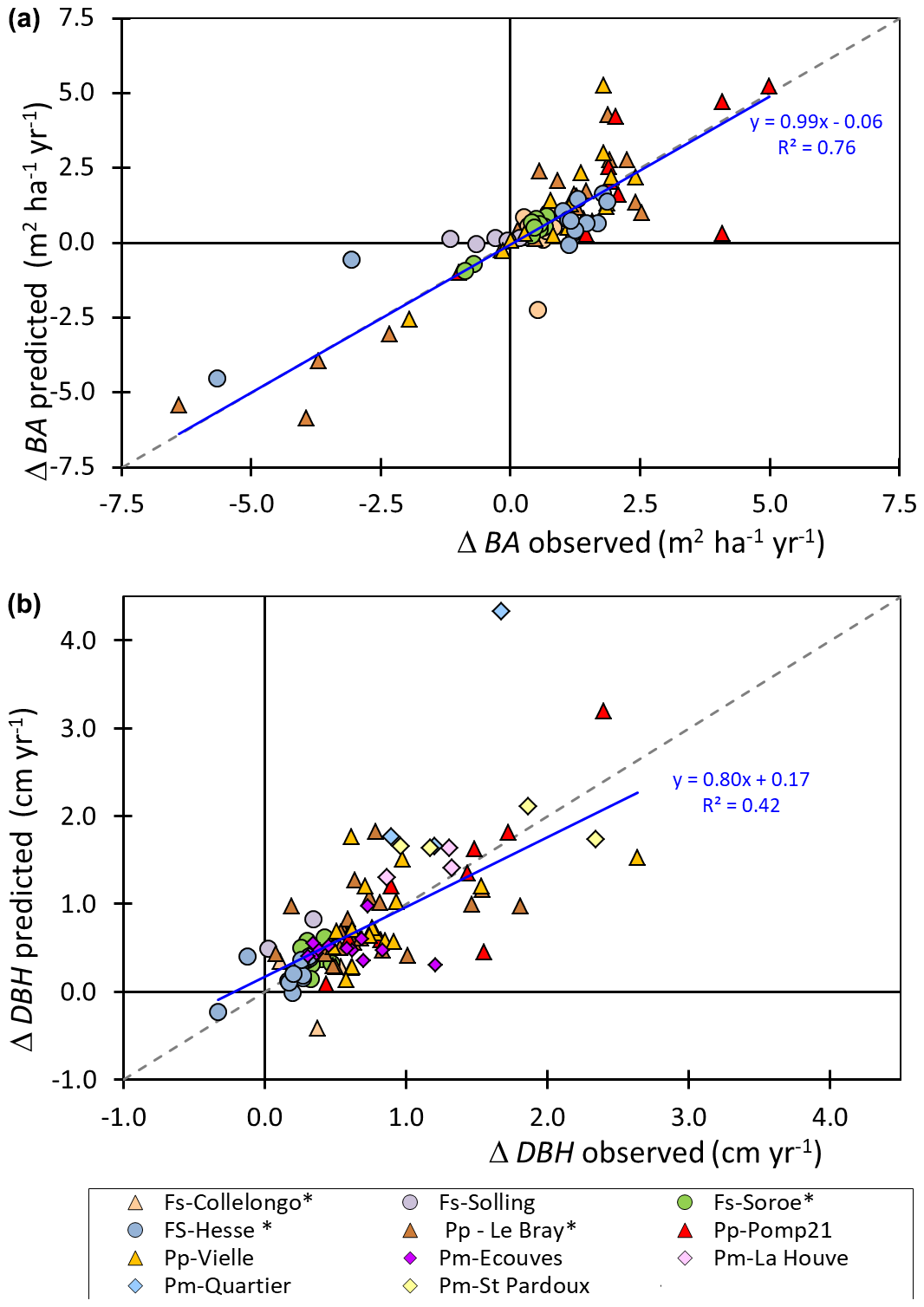
Figure 13Predicted versus observed values of annual increment in basal area, ΔBA (a), and stem mean diameter, ΔD130 (b), for sites described in Table S6 in the Supplement. The sites used for both flux and inventory data are annotated with a star (*). The 1:1 line (dashed line) and linear regression (blue) are shown.
An interesting product of the Go+ model is its evaluation based upon simultaneous values observed and predicted of several variables over decades-long time series. To our knowledge few models have been tested using long-term sets of multiple variables. Figure 14 shows an example for the Collelongo broadleaf forest, Vancouver Island Douglas Fir stand and the Le Bray coniferous forest. In Collelongo and Le Bray, 20- and 25-year-long inventories of tree diameters were available, respectively. A series of soil water stock – or groundwater level – and flux measurements was also available at the three sites. The comparison shows that the long-term trajectory of energy, water and carbon fluxes as well as soil water, tree growth and LAI were captured without significant bias by the model for a period marked by severe droughts (2002 and 2005), a heatwave (2003), several thinnings (1992, 1997, 2005 at Le Bray) and storm damage (at Le Bray 20 % of trees suffered windthrow in December 1999). Some inconsistencies are also evident, such as the overestimation of respiration and primary production at Collelongo, that may be related to LAI overestimation. The behaviour of the soil moisture predicted at the Douglas fir site is also challenged by the observations when soil becomes close to saturation. Because we did not calibrate the parameters for every site, these discrepancies are mainly caused by errors in the values of influential parameters such as the soil depth and hydraulic parameters, the leaf mass-to-area ratio or the root ∕ shoot ratio. The comparison of multiple variables between observed and predicted values also reveals that the performance of the model was clearly affected by the quality of observed flux data. At Le Bray, the flux values were more scattered after 2003 due to a change in instrumentation (closed-path analyser until 2003; open-path from 2004 onward) and related quality assessment criteria: the R2 of the predicted versus observed values of NEE was 0.36 for the period 1997–2003 but dropped to 0.22 when calculated for the entire period 1997–2008. Testing the model against data of different quality levels also produced substantial differences, up to 0.15, in the calculated value of R2.
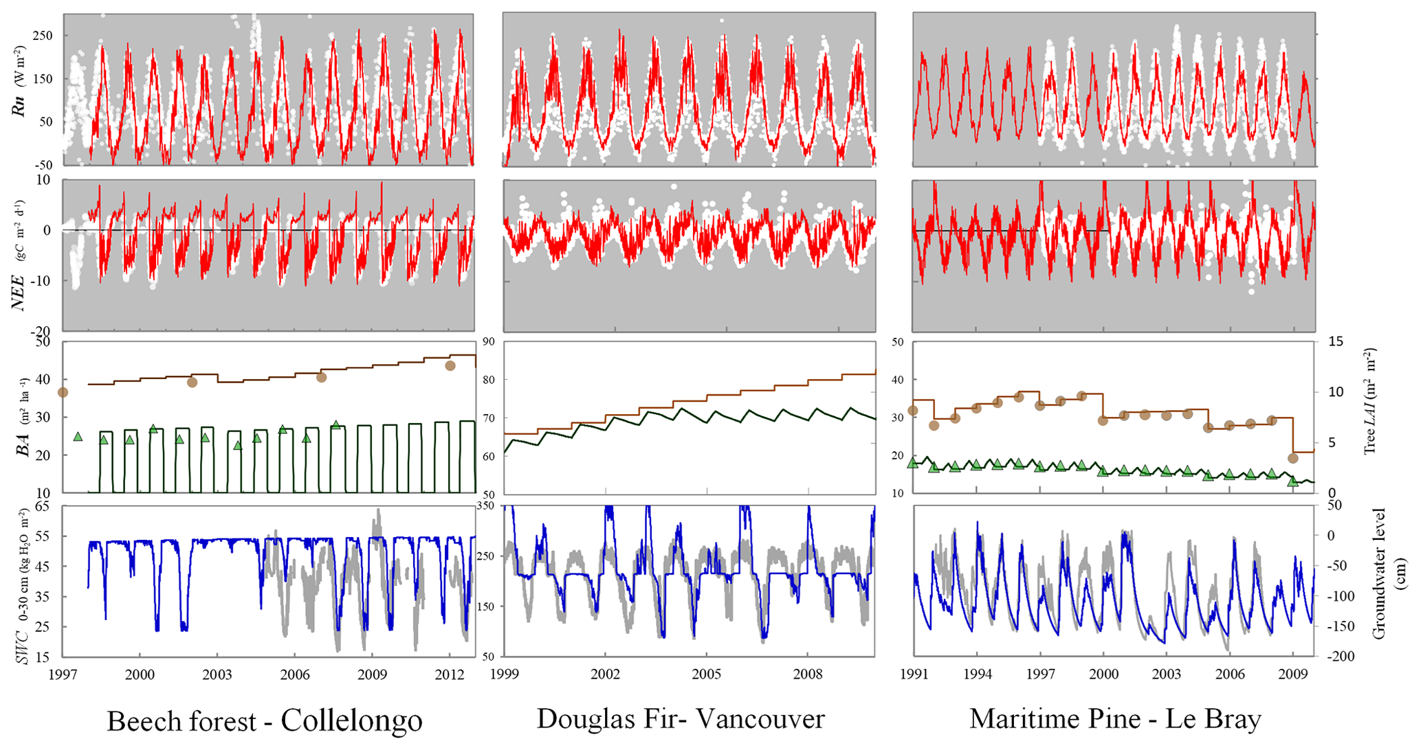
Figure 14Time series of net radiation and CO2 fluxes observed (symbols and grey lines) and predicted (coloured lines), top two rows, together with stand basal area, leaf area index and soil water stock or groundwater level, bottom two rows. Left: Collelongo European beech forest. Centre: Douglas fir stand in British Columbia. Right: Le Bray pine forest. Sources of the data used are detailed in Table 4. The model was initiated in 1997 for the Collelongo experiment, 1998 in the Douglas fir and 1987 for the Le Bray experiment. The soil water content in the top 30 or 60 cm observed at the Collelongo or Douglas fir sites (left axis of bottom row) is compared with soil water content (SWC) in the rooted zone simulated by GO+. At the Le Bray site, the groundwater level is compared for the 1994–2008 period (right axis).
Essentially, the GO+ model brings together robust representations of canopy and carbon cycle processes that can be evaluated straightforwardly against observed data. From a biogeochemical point of view it offers three main innovations: (i) GO+ explicitly links the stomatal functioning of the tree canopy to the leaf water potential and plant hydraulics; (ii) it allows us to connect fast biophysical and biogeochemical processes to slower plant growth and soil carbon transformation processes; and (iii) it provides for a range of options in specifying management operations and harvest exportation for monospecific forest stands. In this section, we first discuss these three points and further model specificities. We then return to a discussion of model performance. First, the tree hydraulics model accounts for the effect of the mean tree height and therefore reflects the effects of age on the leaf water potential and stomatal conductance (Delzon et al., 2005). The hydraulic scheme is kept as simple as possible allowing the description of leaf water potential to be calculated dynamically as a function of transpiration and soil water. The water potential function of canopy stomatal conductance (Eq. 13) is close to Mencuccini et al. (2015) model, the stomatal closure being smoother in our case. The GO+ stomatal conductance model includes three essential features of the soil-to-leaf water transport, i.e. (i) the soil water potential and conductance dependencies on water content (Eqs. S16 and 21), (ii) the relationship between the tree hydraulic conductance and tree height (Eq. 20), and (iii) its capacitance in relation to the total biomass. We think it is a satisfying compromise between more sophisticated models, which would be difficult to parameterize and calibrate at large spatial scales, and the need for describing the temporal fluctuations of leaf water potential and related effects on stomatal conductance. Second, the GO+ net primary production allocation scheme among trees and within tree parts satisfies the need to simulate realistically the tree stand size distribution and the harvested wood product categories. This is required for coupling GO+ to models of wood product life cycles and thus route raw harvest products into a range of product categories, namely pulp, biofuel, industrial products, furniture and construction (Pichancourt et al., 2018). The allocation scheme is sensitive to the environmental stresses and management and satisfies the mass conservation principle. Although simple, this allocation scheme has proven its ability to realistically simulate the dynamics of size distribution in monospecific stands where the selection of trees thinned is crucial (not shown). It summarizes the end result of the carbon transfer processes within a tree. A mechanistic simulation of carbohydrate transport within trees at large spatial scales is still beyond computational capacity and constitutes a research challenge (Mencuccini et al., 2015).The inclusion of a species-specific set of allometric equations is therefore a trade-off allowing us to constrain the growth allocation within trees. It is relatively parsimonious in terms of parameters, yet confers to GO+ a capacity to account for a variety of forest tree species. Moreover, tree allometric equations and parameter values are available for the main tree species of the tropical, temperate and boreal zones (Chave et al., 2014; Forrester et al., 2017). In addition, the prediction of tree size allows the assessment of model performance with data covering a range of temporal scales from hourly to the complete forest rotation time (Thum et al., 2017) as illustrated by its evaluation at the Collelongo and Le Bray sites. The dynamic allocation scheme implemented in the understorey vegetation results in a temporal dynamics that are consistent with our current understanding of understorey vegetation growth in managed stands but could not be evaluated yet at a large spatial scale because of data paucity. Unfortunately, long time series of the annual tree growth for the entire population of trees are still rare and difficult to obtain.
Third, most current practices of forest management in monospecific stands are implemented in the GO+ v3.0 code and can be combined in a wealth of forest management options, including the drainage (not shown) and mechanical preparation of soil, control of vegetation, thinning, coppicing and clear-cutting of the tree stand. The model is being further developed to allow it to simulate tree stands that are not even-aged and mix two to three tree species. Other process-based models also account for a variety of forestry practices (ORCHIDEE-FM; Bellassen et al., 2011; Reyer et al., 2014), but rarely with documented impacts on soil carbon or how the carbon is apportioned to the different harvested products. Regarding the soil carbon, the Roth-C model and its subsequent development, ECOSSE, has been proven to be useful and relatively accurate for estimating the dynamics of carbon in the top 1.0 m of the soil following afforestation (Romanya et al., 2000; Dondini et al., 2015) or in temperate forests under different climate change scenarios (Smith et al., 2006). The adaptation of the ROTH-C model to include the effects of soil mechanical disturbances, as implemented in the GO+ model, substantially improves the predictions of soil carbon changes observed following clear-cutting in the pine forests of southwest France. Nevertheless, the model still has to be evaluated at a large scale. It is worth noting the GO+ code inherently accounts for the light resource competition between trees and understorey. By construction, the access of the vegetation foliage to light is prioritized from the top to the bottom of the canopy allowing the ground vegetation to respond to thinning and to recover first after clear-cutting. The tree layer subsequently dominates when trees have regrown. This version of the GO+ model also suffers from a number of limitations. It does not yet include a biogeochemistry module and does not allow us to simulate mixed-stand forests or stands that are not even-aged; this is because so far very few evaluation datasets are available. The uptake of water from the soil is not prioritized, with understorey vegetation and trees having access to the same soil volume and their transpiration being withdrawn from the soil simultaneously. Both this limitation, and the canopy and soil layers homogeneity assumption, could be overcome in subsequent versions of this model through adding a dynamic partitioning of the canopy and rooted soil. When necessary, the number of layers could also be increased to some extent provided observed data exist to calibrate and validate the canopy structure and simplifying assumptions required. However, de Pury and Farquhar's radiation and photosynthesis canopy model has proven effective as compared with complex multi-layer models and may well suffice for simulating more complex canopies.
With the above limitations in mind, the overall sensitivity profile of the model is consistent with the current understanding of the role of the different processes involved and their functional hierarchy. The sensitivity analysis demonstrates an interaction between the sensitivity of variables with the climate – the water-holding capacity of soil being limiting under dry conditions, i.e. the year 2005 at Le Bray, and the photosynthetic quantum and carboxylation efficiencies becoming the most influential parameters on wet soil. We have also shown how the timescale modifies the sensitivity profile of the model due to the cumulative effects of the fluxes of carbon, energy and water on the stand growth and canopy structure. The GO+ model simulates the seemingly contradictory sensitivity of the autotrophic and heterotrophic respiration to temperature between the short-term (positive direct thermal) effect and the long-term (neutral or negative) effect, which is linked to reduced productivity (Janssens et al., 2001; Atkin and Tjoelker, 2003; Knorr et al., 2005). Although simple, the mechanistic link established between instantaneous canopy processes (radiation and energy balance, transpiration, assimilation and respiration) and longer-term processes, such as primary and secondary stem growth, wood production, and soil carbon and water dynamics, allows us to capture dynamically the main trajectory and energy, water, and carbon fluxes and stocks over decades. The main limitation of our model in that respect is the time resolution of the tree growth processes, which does not account for the seasonality of growth in tree biomass, height and diameter and may therefore introduce errors, e.g. when predicting the autotrophic respiration at an hourly time step. This gap may induce some errors for very fast-growing species but not for slower-growing tree species, as shown in Fig. S3 for the allometric parameters. The sensitivity analysis of GO+ demonstrates that the dynamic representation of stand growth processes is a key feature for capturing the ecosystem behaviour in the long term. We are aware that the conclusions drawn depend on the sensitivity experiment chosen, in terms of climate, soil, tree species and canopy structure, but we think they will be applicable beyond the specific case examined here, at least for canopies with persistent foliage. Whereas the model performances for energy, water vapour and CO2 flux predictions may compare with other current models (Davi et al., 2005; Collalti et al., 2016; Chen et al., 2016), an essential feature of GO+ is its ability to also capture the long-term trends in tree and stand growth and at the same time produce a realistic prediction of the dynamics of understorey vegetation (not shown) and soil carbon. A shift in influence of meteorological variables at day–month scales to biological factors at yearly resolution and beyond was observed by Delpierre et al. (2012) and Stoy et al. (2005, 2009) for many ecosystems through spectral analysis of NEE, GPP and ecosystem respiration sensitivity. This observation suggests the importance of the processes controlling the vegetation dynamics such as phenology, management, growth, and mortality, that are currently described in the GO+ v3.0 model. The accuracy of the model assessed against flux data may appear relatively poor, but it should be noted that a single set of parameter values was used and no site-specific calibration was made. In addition, the most influential site characteristics, the rooting depth and soil hydraulic properties, are unfortunately prone to substantial errors because of the difficulty in determining them and being subject to large spatial variations at the scale of the footprint of flux measurements. Careful examination of the kinetics of predicted and observed flux values reveals that the modelled phenology was not a substantial source of error despite the fact that this process is poorly documented and difficult to parameterize for species such as European beech or maritime pine. Increasing the complexity of the canopy representation, e.g. by taking into account the heterogeneity of sources and sinks within the vegetation layers, might improve the energy balance and flux modelling (see, e.g., Naudts et al., 2015), but at the expense of the model's ability to simulate sites where no such information is available. Considering the diversity of data sources used for evaluation, the model does not show major discrepancies from observations and performed relatively well, with low biases, at simulating the observed values of atmospheric exchanges, tree growth, and soil carbon and water stock changes. The satisfactory results obtained from the comparison with long-term historical series of tree and stand growth and soil carbon and water are particularly promising because they confirm the model's ability to capture low-frequency variations in forest ecosystem functioning for managed forests and demonstrate its ability to simulate management scenarios under different climate scenarios at a regional scale. We could not identify why the GO+ performance for simulating canopy fluxes was so site dependent. It may be in part attributed to the uneven data quality within and between sites; this may be due to changing instrumentation, data gaps and data processing. Indeed, using data obtained on site (level 3) instead of reconstructed (level 4) quality data produced better performances (not shown). The unique species-specific sets of parameter values used per vegetation layer for all sites may also generate deviations from observed values since most influential plant traits, e.g. SLA, or kN, exhibit substantial spatial and temporal variations that are not accounted for in our model evaluations (Fajardo and Siefert, 2016; Hamada et al., 2016; Bloomfield et al., 2018). Most advanced forest models are more finely tuned for specific processes, e.g. PnET-BGC for forest hydrology (Gbondo-Tugbawa et al., 2001; Pourmokhtarian et al., 2012), ANAFORE for cambial growth and carbohydrate storage (Deckmyn et al., 2008), CANOAK, or ORCHIDEE-CAN for light and turbulence attenuation within the canopy (Harley and Baldocchi 1995; Naudts et al., 2015), but are more restricted in terms of temporal scales, process continuity and exhaustiveness. Very few models that can be run over large gridded datasets can implement canopy processes at an hourly timescale: ORCHIDEE-CAN v1.0 (Naudts et al., 2015; Luyssaert et al., 2018), JULES (Best et al., 2011; Clark et al., 2011) or, optionally, LPJ-Guess v3.0 (Smith et al., 2014). The majority run at a daily timescale; that resolution may impair the sensitivity of non-linear processes to climate and CO2 such as photosynthesis, respiration or stomatal function.
The GO+ model allows us to take a new step forward in developing our understanding of the interactive effects of climate and management on forest ecosystems. The model integrates biophysical, biogeochemical, growth and management processes across a range of temporal scales from hour to century and beyond. It thus integrates short timescales, at which ecophysiological reactions take place, into the temporal framework at which the ecosystem functions, thereby covering the entire forest rotational cycle. The low biases in the model predictions of the exchanges of energy, water and carbon explains the model's ability to capture the long-term trajectory of tree and understorey growth and production, which is essential for modelling managed forests. The substantial set of forest management options included in GO+ allows a wealth of combinations of forest operations to be implemented and tested. We believe that apart from the nutrient cycles, GO+ includes all the key processes that are needed for understanding the interactions of forest with climate through radiation and the energy, water and carbon cycles and their impacts on soil and plants, plant growth, phenology and mortality, and wood product exports.
Table A1List of the prognostic variables of the GO+ v3.0 model. Table is split among the main processes. The entity subscripts T, U and S stand for tree canopy, understorey canopy and soil, respectively. The subscript “t” is for individual trees.
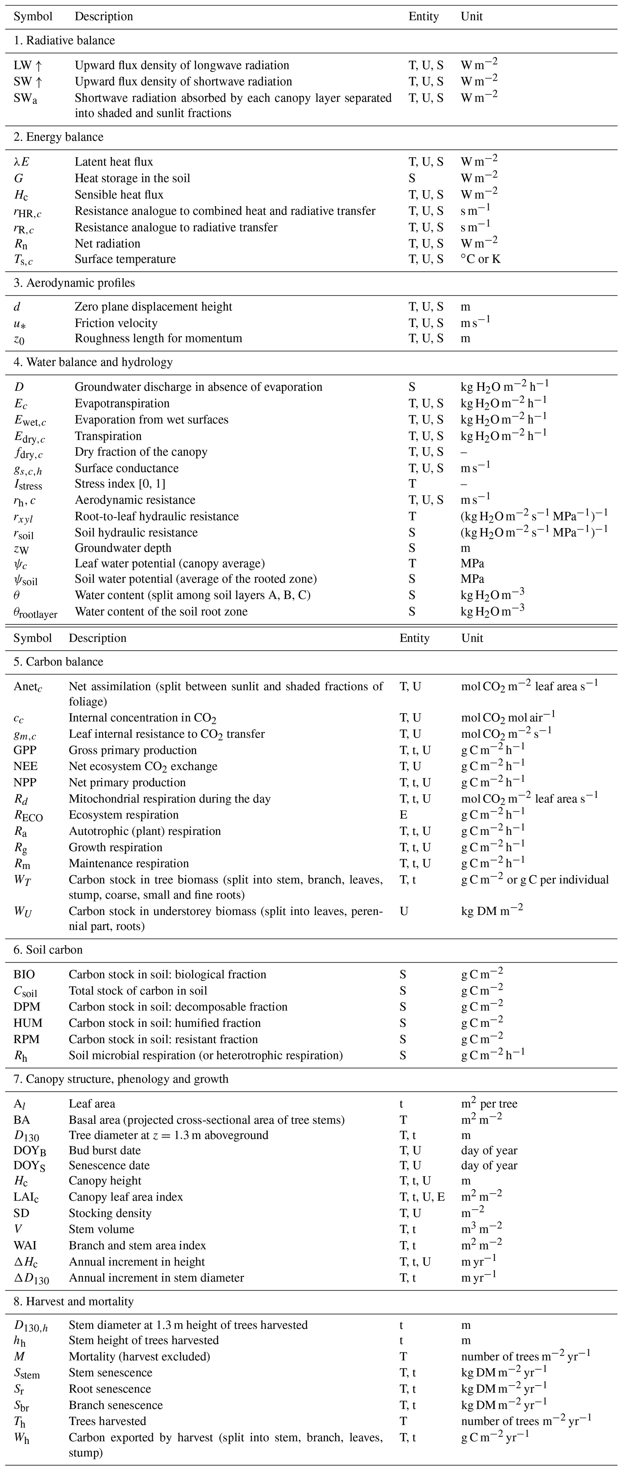
The GO+V3.0 Python code (https://doi.org/10.15454/5K9HCS, Loustau et al., 2020) together with a short user manual and example files (parameters for sites and species, output files, meteorological datasets) can be downloaded from https://github.com/DenisLOUSTAU/GOplus_model_INRAE (last access: 20 April 2020).
The code is also available from the repository https://data.inrae.fr/dataverse/eos (last access: 18 April 2020) although with fewer example files. The data used for evaluating GO+ were from the Fluxnet database located at the European Fluxes Database Cluster (http://gaia.agraria.unitus.it/home, last access: 14 August 2017). The DOI of the datasets of flux sites used are as follows:
-
Le Bray: https://doi.org/10.18140/FLX/1440163 (Berbigier and Loustau, 1996–2008)
-
Collelongo: https://doi.org/10.18140/FLX/1440167 (Matteucci, 1996–2014)
-
Soroe: https://doi.org/10.18140/FLX/1440155 (Ibrom and Pilegaard, 1996–2014).
The forest inventory data used for Douglas fir and partly for maritime pine were provided by the “GIS” data cooperative (Seynave et al., 2018; https://www6.inra.fr/giscoop, last access: 7 June 2017), and by the PROFOUND project database (Reyer et al., 2019; https://doi.org/10.5880/PIK.2019.008, Reyer et al., 2019) for beech forests (Soroe, Collelongo, Solling).
The supplement related to this article is available online at: https://doi.org/10.5194/gmd-13-5973-2020-supplement.
VM developed different modules of the model, the understorey, soil and part of the management, and she synthesized and reviewed the final version of the paper. DA, AB, CC, SM, DP, RV and RA co-developed the model, its adaptation to different species, different modules, and parts of the sensitivity and uncertainly analysis. CM implemented the code over gridded datasets using parallel computing. VB, ATB, JMB, AG, CJ, BL, GM, MN and KP provided the datasets used about the soil carbon, tree and understorey phenology, forest inventories, and canopy fluxes of energy and CO2 and contributed to data analysis and model evaluation. OP and OR led the projects supporting the development of the version 3.0 GO+. They supervised the paper structure, content and layout. DL developed preliminary versions of the model, made the numerical experiments described in the verification and model evaluation sections and wrote the first version of the article.
The authors declare that they have no conflict of interest.
The datasets used for evaluating the GO+ model with stand growth data and tree species phenology were provided by Céline Meredieu (INRAE UEFP0570) for the maritime pine permanent plot, the “GIS Coopérative de données” https://www6.inra.fr/giscoop/ (last access: 7 June 2017) (Douglas fir and maritime pine datasets), French ICP-Forest network (French part of ICP-Forests Level II network Renecofor), and Christopher Reyer (PIK – Potsdam) and the ISI-MIP project for the beech datasets. The datasets of flux measurements were downloaded from the European Data Cluster and Fluxnet (La Thuile 2015 dataset). The authors thank John H. C. Gash for reviewing the English and style of the paper.
This research has been supported by the French National Research Agency (ANR, grant nos. 10-CPL-0011 and 13-AGRO-0005), the Agency for ecological transition (ADEME, grant no.13-60-C0092) and the European Union's Horizon H2020 programme (grant no. 730944).
This paper was edited by Christoph Müller and reviewed by two anonymous referees.
Achat, D. L., Fortin, M., Landmann, G., Ringeval, B., and Augusto, L.: Forest soil carbon is threatened by intensive biomass harvesting, Sci. Rep.-UK, 5, 15991, https://doi.org/10.1038/srep15991, 2015.
Achat, D. L., Martel, S., Picart, D., Moisy, C., Augusto, L., Bakker, M. R., and Loustau, D.: Modelling the nutrient cost of biomass harvesting under different silvicultural and climate scenarios in production forests, Forest Ecol. Manag., 429, 642–653, https://doi.org/10.1016/j.foreco.2018.06.047, 2018.
Ahlswede, B. J. and Thomas, R. Q.: Community earth system model simulations reveal the relative importance of afforestation and forest management to surface temperature in Eastern North America, Forests, 8, 499, https://doi.org/10.3390/f8120499, 2017.
Arrouays, D. and Pelissier, P.: Changes in carbon storage in temperate humic loamy soils after forest clearing and continuous corn cropping in France, Plant Soil, 160, 215–223, 1994.
Atkin, O. K. and Tjoelker, M. G.: Thermal acclimation and the dynamic response of plant respiration to temperature, Trends Plant Sci., 8, 343–351, https://doi.org/10.1016/s1360-1385(03)00136-5, 2003.
Bala, G., Caldeira, K., Wickett, M., Phillips, T. J., Lobell, D. B., Delire, C., and Mirin, A.: Combined climate and carbon-cycle effects of large-scale deforestation, P. Natl. Acad. Sci. USA., 104, 6550–6555, https://doi.org/10.1073/pnas.0608998104, 2007.
Balesdent, J., Besnard, E., Arrouays, D., and Chenu, C.: The dynamics of carbon in particle-size fractions of soil in a forest-cultivation sequence, Plant Soil, 201, 49–57, 1998.
Bellassen, V., Le Maire, G., Dhôte, J. F., Ciais, P., and Viovy, N.: Modelling forest management within a global vegetation model – Part 1: Model structure and general behaviour, Ecol. Modell., 221, 2458–2474, https://doi.org/10.1016/j.ecolmodel.2010.07.008, 2010.
Bellassen, V., le Maire, G., Guin, O., Dhôte, J. F., Ciais, P., and Viovy, N.: Modelling forest management within a global vegetation model – Part 2: Model validation from a tree to a continental scale, Ecol. Modell., 222, 57–75, 2011.
Berbigier, P. and Bonnefond, J. M.: Measurement and Modeling of Radiation Transmission within a Stand of Maritime Pine (Pinus-Pinaster Ait), Ann. For. Sci., 52, 23–42, 1995.
Berbigier, P. and Loustau, D.: FLUXNET2015 FR-LBr Le Bray, Dataset, https://doi.org/10.18140/FLX/1440163, 1996–2008.
Berbigier, P., Bonnefond, J. M., and Mellmann, P.: CO2 and water vapour fluxes for 2 years above Euroflux forest site, Agric. For. Meteorol., 108, 183–197, 2001.
Best, M. J., Pryor, M., Clark, D. B., Rooney, G. G., Essery, R. L. H., Ménard, C. B., Edwards, J. M., Hendry, M. A., Porson, A., Gedney, N., Mercado, L. M., Sitch, S., Blyth, E., Boucher, O., Cox, P. M., Grimmond, C. S. B., and Harding, R. J.: The Joint UK Land Environment Simulator (JULES), model description – Part 1: Energy and water fluxes, Geosci. Model Dev., 4, 677–699, https://doi.org/10.5194/gmd-4-677-2011, 2011.
Betts, R. A.: Offset of the potential carbon sink from boreal forestation by decreases in surface albedo, Nature, 408, 187–190, https://doi.org/10.1038/35041545, 2000.
Bloomfield, K. J., Cernusak, L. A., Eamus, D., Ellsworth, D. S., Prentice, I. C., Wright, I. J., Boer, M. M., Bradford, M. G., Cale, P., Cleverly, J., Egerton, J. J. G., Evans, B. J., Hayes, L. S., Hutchinson, M. F., Liddell, M. J., Macfarlane, C., Meyer, W. S., Prober, S. M., Togashi, H. F., Wardlaw, T., Zhu, L. L., and Atkin, O. K.: A continental-scale assessment of variability in leaf traits: Within species, across sites and between seasons, Funct. Ecol., 32, 1492–1506, 2018.
Borys, A., Suckow, F., Reyer, C., Gutsch, M., and Lasch-Born, P.: The impact of climate change under different thinning regimes on carbon sequestration in a German forest district, Mitig. Adapt. Strat. Gl., 21, 861–881, https://doi.org/10.1007/s11027-014-9628-6, 2016.
Breda, N. J. J.: Ground-based measurements of leaf area index: a review of methods, instruments and current controversies, J. Exp. Bot., 54, 2403–2417, 2003.
Bright, R. M., Cherubini, F., and Strømman, A. H.: Climate impacts of bioenergy: Inclusion of carbon cycle and albedo dynamics in life cycle impact assessment, Environ. Impact Assess. Rev., 37, 2–11, https://doi.org/10.1016/j.eiar.2012.01.002, 2012.
Bright, R. M., Davin, E., O'Halloran, T., Pongratz, J., Zhao, K. G., and Cescatti, A.: Local temperature response to land cover and management change driven by non-radiative processes, Nat. Clim. Change, 7, 296, https://doi.org/10.1038/nclimate3250, 2017.
Campolongo, F. and Saltelli, A.: Sensitivity analysis of an environmental model an application of different analysis methods, Reliab. Eng. Syst. Safe., 57, 49–69, 1997.
Chave, J., Rejou-Mechain, M., Burquez, A., Chidumayo, E., Colgan, M. S., Delitti, W. B., Duque, A., Eid, T., Fearnside, P. M., Goodman, R. C., Henry, M., Martinez-Yrizar, A., Mugasha, W. A., Muller-Landau, H. C., Mencuccini, M., Nelson, B. W., Ngomanda, A., Nogueira, E. M., Ortiz-Malavassi, E., Pelissier, R., Ploton, P., Ryan, C. M., Saldarriaga, J. G., and Vieilledent, G.: Improved allometric models to estimate the aboveground biomass of tropical trees, Global Change Biol., 20, 3177–3190, https://doi.org/10.1111/gcb.12629, 2014.
Chen, C. R., Xu, Z. H., and Mathers, N. J.: Soil carbon pools in adjacent natural and plantation forests of subtropical Australia, Soil Sci. Soc. Am. J., 8, 282–291, https://doi.org/10.2136/sssaj2004.2820, 2004.
Chen, Y., Ryder, J., Bastrikov, V., McGrath, M. J., Naudts, K., Otto, J., Ottlé, C., Peylin, P., Polcher, J., Valade, A., Black, A., Elbers, J. A., Moors, E., Foken, T., van Gorsel, E., Haverd, V., Heinesch, B., Tiedemann, F., Knohl, A., Launiainen, S., Loustau, D., Ogée, J., Vessala, T., and Luyssaert, S.: Evaluating the performance of land surface model ORCHIDEE-CAN v1.0 on water and energy flux estimation with a single- and multi-layer energy budget scheme, Geosci. Model Dev., 9, 2951–2972, https://doi.org/10.5194/gmd-9-2951-2016, 2016.
Ciais, P., Loustau, D., Bosc, A., Ogée, J., Dufrêne, E., François, C., Viovy, N., and Delage, F.: How will the production of French forests respond to climate change? An integrated analysis from site to country scale, in: Forests, carbon cycle and climate change, edited by: Loustau, D., Quae, Paris, 2010.
Clark, D. B., Mercado, L. M., Sitch, S., Jones, C. D., Gedney, N., Best, M. J., Pryor, M., Rooney, G. G., Essery, R. L. H., Blyth, E., Boucher, O., Harding, R. J., Huntingford, C., and Cox, P. M.: The Joint UK Land Environment Simulator (JULES), model description – Part 2: Carbon fluxes and vegetation dynamics, Geosci. Model Dev., 4, 701–722, https://doi.org/10.5194/gmd-4-701-2011, 2011.
Coleman K. and Jenkinson, D. D.: RothC – 26.3 – A model for the turnover of carbon in soil, in: Evaluation of soil organic matter models using existing, long-term dataset, edited by: Powlson, D. S., Smith, P., and Smith, J. U., NATO ASI Series I, Springer Verlag, Heidelberg, Germany, 237–246, 1996.
Collalti, A., Marconi, S., Ibrom, A., Trotta, C., Anav, A., D'Andrea, E., Matteucci, G., Montagnani, L., Gielen, B., Mammarella, I., Grünwald, T., Knohl, A., Berninger, F., Zhao, Y., Valentini, R., and Santini, M.: Validation of 3D-CMCC Forest Ecosystem Model (v.5.1) against eddy covariance data for 10 European forest sites, Geosci. Model Dev., 9, 479–504, https://doi.org/10.5194/gmd-9-479-2016, 2016.
Davi, H., Dufrene, E., Granier, A., Le Dantec, V., Barbaroux, C., Francois, C., and Breda, N.: Modelling carbon and water cycles in a beech forest Part II: Validation of the main processes from organ to stand scale, Ecol. Modell., 185, 387–405, 2005.
Davi, H., Dufrêne, E., Francois, C., Le Maire, G., Loustau, D., Bosc, A., Rambal, S., Granier, A., and Moors, E.: Sensitivity of water and carbon fluxes to climate changes from 1960 to 2100 in European forest ecosystems, Agr. Forest. Meteorol., 141, 35–56, https://doi.org/10.1016/j.agrformet.2006.09.003, 2006.
Deckmyn, G., Verbeeck, H., de Beeck, M. O., Vansteenkiste, D., Steppe, K., and Ceulemans, R.: ANAFORE: A stand-scale process-based forest model that includes wood tissue development and labile carbon storage in trees, Ecol. Modell., 215, 345–368, https://doi.org/10.1016/j.ecolmodel.2008.04.007, 2008.
Delpierre, N., Dufrêne, E., Soudani, K., Ulrich, E., Cecchini, S., Boé, J., and François, C.: Modelling interannual and spatial variability of leaf senescence for three deciduous tree species in France, Agr. Forest. Meteorol., 149, 938–948, https://doi.org/10.1016/j.agrformet.2008.11.014, 2009.
Delpierre, N., Soudani, K., Francois, C., Le Maire, G., Bernhofer, C., Kutsch, W., Misson, L., Rambal, S., Vesala, T., and Dufrene, E.: Quantifying the influence of climate and biological drivers on the interannual variability of carbon exchanges in European forests through process-based modelling, Agr. Forest Meteorol., 154, 99–112, https://doi.org/10.1016/j.agrformet.2011.10.010, 2012.
Delzon, S. and Loustau, D.: Age-related decline in stand water use: sap flow and transpiration in a pine forest chronosequence, Agr. Forest Meteorol., 129, 105–119, https://doi.org/10.1016/j.agrformet.2005.01.002, 2005.
Delzon, S., Sartore, M., Burlett, R., Dewar, R., and Loustau, D.: Hydraulic responses to height growth in maritime pine trees, Plant Cell Environ., 27, 1077–1087, 2004.
de Pury, D. G. G. and Farquhar, G. D.: Simple scaling of photosynthesis from leaves to canopies without the errors of big-leaf models, Plant Cell Environ., 20, 537–557, 1997.
Dobarco, M. R., Cousin, I., Le Bas, C., and Martin, M. P.: Pedotransfer functions for predicting available water capacity in French soils, their applicability domain and associated uncertainty, Geoderma, 336, 81–95, 2019.
Dondini, M., Jones, E. O., Richards, M., Pogson, M., Rowe, R. L., Keith, A. M., Perks, M. P., McNamara, N. P., Smith, J. U., and Smith, P.: Evaluation of the ECOSSE model for simulating soil carbon under short rotation forestry energy crops in Britain, GCB Bioenergy, 7, 527–540, https://doi.org/10.1111/gcbb.12154, 2015.
Dufrene, E., Davi, H., Francois, C., le Maire, G., Le Dantec, V., and Granier, A.: Modelling carbon and water cycles in a beech forest Part I: Model description and uncertainty analysis on modelled NEE, Ecol. Modell., 185, 407–436, 2005.
Ellsworth, D. S., Crous, K. Y., Lambers, H., and Cooke, J.: Phosphorus recycling in photorespiration maintains high photosynthetic capacity in woody species, Plant Cell Environ., 38, 1142–1156, 2015.
Erb, K.-H., Kastner, T., Plutzar, C., Bais, A. L. S., Carvalhais, N., Fetzel, T., Gingrich, S., Haberl, H., Lauk, C., Niedertscheider, M., Pongratz, J., Thurner, M., and Luyssaert, S.: Unexpectedly large impact of forest management and grazing on global vegetation biomass, Nature, 553, 73–76, 2017.
Fajardo, A. and Siefert, A.: Phenological variation of leaf functional traits within species, Oecologia, 180, 951–959, 2016.
Farquhar, G. D., von Caemmerer, S., and Berry, J.: A biochemical model of photosynthetic CO2 assimilation in leaves of C3 species, Planta, 149, 78–90, 1980.
Felzer, B. S. and Jiang, M.: Effect of Land Use and Land Cover Change in Context of Growth Enhancements in the United States Since 1700: Net Source or Sink?, J. Geophys. Res.-Biogeo., 123, 3439–3457, 2018.
Forrester, D. I., Tachauer, I. H. H., Annighoefer, P., Barbeito, I., Pretzsch, H., Ruiz-Peinado, R., Stark, H., Vacchiano, G., Zlatanov, T., Chakraborty, T., Saha, S., and Sileshi, G. W.: Generalized biomass and leaf area allometric equations for European tree species incorporating stand structure, tree age and climate, Forest Ecol. Manag., 396, 160–175, https://doi.org/10.1016/j.foreco.2017.04.011, 2017.
Garcia, M., Ozdogan, M., and Townsend, P. A.: Impacts of forest harvest on cold season land surface conditions and land-atmosphere interactions in northern Great Lakes states, J. Adv. Model. Earth Sy., 6, 923–937, https://doi.org/10.1002/2014ms000317, 2014.
Gash, J. H. C.: Analytical model of rainfall interception by forests, Q. J. Roy. Meteor. Soc., 105, 43–55, https://doi.org/10.1002/qj.49710544304, 1979.
Gbondo-Tugbawa, S. S., Driscoll, C. T., Aber, J. D., and Likens, G. E.: Evaluation of an integrated biogeochemical model (PnET-BGC) at a northern hardwood forest ecosystem, Water Resour. Res., 37, 1057–1070, https://doi.org/10.1029/2000WR900375, 2001.
Ghanbarian-Alavijeh, B., Liaghat, A., Huang, G.-H., and Van Genuchten, M. T.: Estimation of the van Genuchten Soil Water Retention Properties from Soil Textural Data, Pedosphere, 20, 456–465, 2010.
Gholz, H. L.: Limits on aboveground net primary production, leaf area, and biomass in vegetational zones of the Pacific Northwest, Dissertation, Oregon State University, Corvallis, Oregon, USA, 1979.
Gottschalk, P., Bellarby, J., Chenu, C., Foereid, B., Smith, P., Wattenbach, M., Zingore, S., and Smith, J.: Simulation of soil organic carbon response at forest cultivation sequences using C-13 measurements, Org. Geochem., 41, 41–54, https://doi.org/10.1016/j.orggeochem.2009.04.017, 2010.
Granier, A. and Bréda, N.: Modelling canopy conductance and stand transpiration of an oak forest from sap flow measurements, Ann. For. Sci., 53, 537–546, 1996.
Granier, A. and Loustau, D.: Measuring and modelling the transpiration of a maritime pine canopy from sap-flow data, Agr. Forest. Meteorol., 71, 61–81, 1994.
Granier, A., Ceschia, E., Damesin, C., Dufrene, E., Epron, D., Gross, P., Lebaube, S., Le Dantec, V., Le Goff, N., Lemoine, D., Lucot, E., Ottorini, J. M., Pontailler, J. Y., and Saugier, B.: The carbon balance of a young Beech forest, Funct. Ecol., 14, 312–325, 2000a.
Granier, A., Loustau, D., and Bréda, N.: A generic model of forest canopy conductance dependent of climate, soil water availability and leaf area index, Ann. For. Sci., 57, 755–765, 2000b.
Grassi, G., House, J., Dentener, F., Federici, S., den Elzen, M., and Penman, J.: The key role of forests in meeting climate targets requires science for credible mitigation, Nat. Clim. Change, 7, 220–226, 2017.
Griscom, B. W., Adams, J., Ellis, P. W., Houghton, R. A., Lomax, G., Miteva, D. A., Schlesinger, W. H., Shoch, D., Siikamaki, J. V., Smith, P., Woodbury, P., Zganjar, C., Blackman, A., Campari, J., Conant, R. T., Delgado, C., Elias, P., Gopalakrishna, T., Hamsik, M. R., Herrero, M., Kiesecker, J., Landis, E., Laestadius, L., Leavitt, S. M., Minnemeyer, S., Polasky, S., Potapov, P., Putz, F. E., Sanderman, J., Silvius, M., Wollenberg, E., and Fargione, J.: Natural climate solutions, P. Natl. Acad. Sci. USA., 114, 11645–11650, https://doi.org/10.1073/pnas.1710465114, 2017.
Guillemot, J., Delpierre, N., Vallet, P., François, C., Martin-StPaul, N. K., Soudani, K., Nicolas, M., Badeau, V., and Dufrêne, E.: Assessing the effects of management on forest growth across France: insights from a new functional–structural model, Ann. Bot., 114, 779–793, https://doi.org/10.1093/aob/mcu059, 2014.
Gutsch, M., Lasch, P., Suckow, F., and Reyer, C.: Management of mixed oak-pine forests under climate scenario uncertainty, Forest Syst., 20, 453–463, https://doi.org/10.5424/fs/20112003-11073, 2011.
Hamada, S., Kumagai, T., Kochi, K., Kobayashi, N., Hiyama, T., and Miyazawa, Y.: Spatial and temporal variations in photosynthetic capacity of a temperate deciduous-evergreen forest, Trees-Structure and Function, 30, 1083–1093, 2016.
Harley, P. C. and Baldocchi, D. D.: Scaling carbon-dioxide and water-vapour exchange from leaf to canopy in a deciduous forest .1. Leaf model parameterization, Plant. Cell Environ., 18, 1146–1156, https://doi.org/10.1111/j.1365-3040.1995.tb00625.x, 1995.
Harper, A. B., Wiltshire, A. J., Cox, P. M., Friedlingstein, P., Jones, C. D., Mercado, L. M., Sitch, S., Williams, K., and Duran-Rojas, C.: Vegetation distribution and terrestrial carbon cycle in a carbon cycle configuration of JULES4.6 with new plant functional types, Geosci. Model Dev., 11, 2857–2873, https://doi.org/10.5194/gmd-11-2857-2018, 2018.
Hassika, P., Berbigier, P., and Bonnefond, J. M.: Measurement and modelling of the photosynthetically active radiation transmitted in a canopy of maritime pine, Ann. For. Sci., 54, 715–730, 1997.
Huang, L., Zhai, J., Liu, J. Y., and Sun, C. Y.: The moderating or amplifying biophysical effects of afforestation on CO2-induced cooling depend on the local background climate regimes in China, Agr. Forest. Meteorol., 260, 193–203, https://doi.org/10.1016/j.agrformet.2018.05.020, 2018.
Humphreys, E. R., Black, T. A., Morgenstern, K., Cai, T., Drewitt, G. B., Nesic, Z., and Trofymow, J. A.: Carbon dioxide fluxes in coastal Douglas-fir stands at different stages of development after clearcut harvesting, Agr. Forest Meteorol., 140, 6–22, 2006.
Ibrom, A. and Pilegaard, K.: FLUXNET2015 DK-Sor Soroe, Dataset, https://doi.org/10.18140/FLX/1440155, 1996–2014.
IPCC: Climate Change and Land. An IPCC special report on climate change, desertification, land degradation, sustainable land management, food security, and greenhouse gas fluxes in terrestrial ecosystems, available at: https://www.ipcc.ch/srccl-report-download-page/, last access: 19 September 2019.
Janssens, I. A., Lankreijer, H., Matteucci, G., Kowalski, A. S., Buchmann, N., Epron, D., Pilegaard, K., Kutsch, W., Longdoz, B., Grunwald, T., Montagnani, L., Dore, S., Rebmann, C., Moors, E. J., Grelle, A., Rannik, U., Morgenstern, K., Oltchev, S., Clement, R., Gudmundsson, J., Minerbi, S., Berbigier, P., Ibrom, A., Moncrieff, J., Aubinet, M., Bernhofer, C., Jensen, N. O., Vesala, T., Granier, A., Schulze, E. D., Lindroth, A., Dolman, A. J., Jarvis, P. G., Ceulemans, R., and Valentini, R.: Productivity overshadows temperature in determining soil and ecosystem respiration across European forests, Global Change Biol., 7, 269–278, https://doi.org/10.1046/j.1365-2486.2001.00412.x, 2001.
Jarvis, P. G.: The interpretation of the variation in leaf water potential and stomatal conductance found in canopies in the field, Phil. Trans. R. Soc. B, 273, 593–610, 1976.
Jolivet, C.: Le carbone organique des sols des Landes de Gascogne variabilité spatiale et effets des pratiques sylvicoles et agricoles, PhD Thesis, Université de Bourgogne, Dijon, 306 pp., 2000.
Jones, H. G.: Plants and microclimate: a quantitative approach to environmental plant physiology, Cambridge University Press, Cambridge, 1992.
Jurevics, A., Peichl, M., Olsson, B. A., Stromgren, M., and Egnell, G.: Slash and stump harvest have no general impact on soil and tree biomass C pools after 32–39 years, Forest Ecol. Manag., 371, 33–41, https://doi.org/10.1016/j.foreco.2016.01.008, 2016.
Karjalainen, T., Pussinen, A., Liski, J., Nabuurs, G. J., Eggers, T., Lapvetelainen, T., and Kaipainen, T.: Scenario analysis of the impacts of forest management and climate change on the European forest sector carbon budget, Forest Policy Econ, 5, 141–155, 2003.
Knorr, W., Prentice, I. C., House, J. I., and Holland, E. A.: Long-term sensitivity of soil carbon turnover to warming, Nature, 433, 298–301, https://doi.org/10.1038/nature03226, 2005.
Kurz, W. A., Dymond, C. C., White, T. M., Stinson, G., Shaw, C. H., Rampley, G. J., Smyth, C., Simpson, B. N., Neilson, E. T., Tyofymow, J. A., Metsaranta, J., and Apps, M. J.: CBM-CFS3: A model of carbon-dynamics in forestry and land-use change implementing IPCC standards, Ecol. Modell., 220, 480–504, 2009.
Kuusinen, N., Lukes, P., Stenberg, P., Levula, J., Nikinmaa, E., and Berninger, F.: Measured and modelled albedos in Finnish boreal forest stands of different species, structure and understory, Ecol. Modell., 284, 10–18, https://doi.org/10.1016/j.ecolmodel.2014.04.007, 2014.
Landsberg, J. J. and Waring, R. H.: A generalised model of forest productivity using simplified concepts of radiation-use efficiency, carbon balance and partitioning, Forest Ecol. Manag., 95, 209–228, 1997.
Lebourgeois, F., Pierrat, J.-C., Perez, V., Piedallu, C., Cecchini, S., Ulrich, E.: Phenological timing in French temperate forests – a study on stands in the renecofor network, Revue Forestiere Française, 60, 323–343, 2008.
Lee, X., Goulden, M. L., Hollinger, D. Y., Barr, A., Black, T. A., Bohrer, G., Bracho, R., Drake, B., Goldstein, A., Gu, L. H., Katul, G., Kolb, T., Law, B. E., Margolis, H., Meyers, T., Monson, R., Munger, W., Oren, R., Kyaw, T. P. U., Richardson, A. D., Schmid, H. P., Staebler, R., Wofsy, S., and Zhao, L.: Observed increase in local cooling effect of deforestation at higher latitudes, Nature, 479, 384–387, https://doi.org/10.1038/nature10588, 2011.
Le Moguedec, G. and Dhôte, J. F.: Fagacees: a tree-centered growth and yield model for sessile oak (Quercus petraea L.) and common beech (Fagus sylvatica L.), Ann. For. Sci., 69, 257–269, 2012.
Lindner, M., Bugmann, H., Lasch, P., Flechsig, M., and Cramer, W.: Regional impacts of Clim. Change on forests in the state of Brandenburg, Germany, Agr. Forest. Meteorol., 84, 123–135, 10.1016/s0168-1923(96)02381-7, 1997.
Loustau, D. and Cochard, H.: Use of a portable transpiration chamber for estimating evapotranspiration in the Molinia caerulea understorey of a maritime pine stand, Ann. For. Sci., 48, 29–45, 1991.
Loustau, D., Berbigier, P., Roumagnac, P., Ferreira, M. I., Pereira, J. S., Arruda-Pacheco, C., David, J. S., and Tavares, R.: Transpiration of a 64-year-old maritime pine stand in Portugal. I: Seasonal course of water flux through maritime pine, Oecologia, 107, 33–42, 1996.
Loustau, D., Domec, J. C., and Bosc, A.: Interpreting the variations in xylem sap flux density within the trunk of maritime pine (Pinus pinaster Ait.): application of a model for calculating water flows at tree and stand levels, Ann. For. Sci., 55, 29–46, 1998.
Loustau, D., Bosc, A., Colin, A., Ogee, J., Davi, H., Francois, C., Dufrene, E., Deque, M., Cloppet, E., Arrouays, D., Le Bas, C., Saby, N., Pignard, G., Hamza, N., Granier, A., Breda, N., Ciais, P., Viovy, N., and Delage, F.: Modeling climate change effects on the potential production of French plains forests at the sub-regional level, Tree Physiol., 25, 813–823, 2005.
Loustau, D., Moisy, C., Bosc, A., Figuères, S., Martel, S., Moreaux, V., and Picart-Deshors, D.: GO+ v3.0 model code, Portail Data INRAE, V2, https://doi.org/10.15454/5K9HCS, 2020.
Luyssaert, S., Jammet, M., Stoy, P. C., Estel, S., Pongratz, J., Ceschia, E., Churkina, G., Don, A., Erb, K., Ferlicoq, M., Gielen, B., Grunwald, T., Houghton, R. A., Klumpp, K., Knohl, A., Kolb, T., Kuemmerle, T., Laurila, T., Lohila, A., Loustau, D., McGrath, M. J., Meyfroidt, P., Moors, E. J., Naudts, K., Novick, K., Otto, J., Pilegaard, K., Pio, C. A., Rambal, S., Rebmann, C., Ryder, J., Suyker, A. E., Varlagin, A., Wattenbach, M., and Dolman, A. J.: Land management and land-cover change have impacts of similar magnitude on surface temperature, Nat. Clim. Change, 4, 389–393, https://doi.org/10.1038/nclimate2196, 2014.
Luyssaert, S., Marie, G., Valade, A., Chen, Y.-Y., Njakou Djomo, S., Ryder, J., Otto, J., Naudts, K., Lansø, A. S., Ghattas, J., and McGrath, M. J.: Trade-offs in using European forests to meet climate objectives, Nature, 562, 259–262, https://doi.org/10.1038/s41586-018-0577-1, 2018.
Masera, O. R., Garza-Caligaris, J. F., Kanninen, M., Karjalainen, T., Liski, J., Nabuurs, G. J., Pussinen, A., de Jong, B. H. J., and Mohren, G. M. J.: Modeling carbon sequestration in afforestation, agroforestry and forest management projects: the CO2FIX V.2 approach, Ecol. Modell., 164, 177–199, 2003.
Matteucci, G.: FLUXNET2015 IT-Col Collelongo, Dataset, https://doi.org/10.18140/FLX/1440167, 1996–2014.
Medlyn, B. E., Barton, C. V. M., Broadmeadow, M. S. J., Ceulemans, R., De Angelis, P., Forstreuter, M., Freeman, M., Jackson, S. B., Kellomaki, S., Laitat, E., Rey, A., Roberntz, P., Sigurdsson, B. D., Strassemeyer, J., Wang, K., Curtis, P. S., and Jarvis, P. G.: Stomatal conductance of forest species after long-term exposure to elevated CO2 concentration: a synthesis, New Phytol., 149, 247–264, 2001.
Medlyn, B. E., Dreyer, E., Ellsworth, D., Forstreuter, M., Harley, P. C., Kirschbaum, M. U. F., Le Roux, X., Montpied, P., Strassemeyer, J., Walcroft, A., Wang, K., and Loustau, D.: Temperature response of parameters of a biochemically based model of photosynthesis. II. A review of experimental data, Plant Cell Environ., 25, 1167–1179, 2002.
Medlyn, B. E., Berbigier, P., Clement, R., Grelle, A., Loustau, D., Linder, S., Wingate, L., Jarvis, P. G., Sigurdsson, B. D., and McMurtrie, R. E.: Carbon balance of coniferous forests growing in contrasting climates: Model-based analysis, Agric. Forest Meteorol., 131, 97–124, 2005.
Mencuccini, M., Minunno, F., Salmon, Y., Martínez-Vilalta, J., and Hölttä, T.: Coordination of physiological traits involved in drought-induced mortality of woody plants, New Phytol., 208, 396–409, https://doi.org/10.1111/nph.13461, 2015.
Moffat, A. M., Papale, D., Reichstein, M., Hollinger, D. Y., Richardson, A. D., Barr, A. G., Beckstein, C., Braswell, B. H., Churkina, G., Desai, A. R., Falge, E., Gove, J. H., Heimann, M., Hui, D. F., Jarvis, A. J., Kattge, J., Noormets, A., and Stauch, V. J.: Comprehensive comparison of gap-filling techniques for eddy covariance net carbon fluxes, Agric. Forest Meteorol., 147, 209–232, 2007.
Moreaux, V.: Observation et modélisation des échanges d'énergie et de masse de jeunes peuplements forestiers du Sud-Ouest de la France, PhD thesis, Ecole Doctorale 304 “Sciences et Environnements”, Thématique “Physique de l'Environnement”, Université de Bordeaux-1, Bordeaux, 262 pp., 2012.
Moreaux, V., Lamaud, E., Bosc, A., Bonnefond, J.-M., Medlyn, B. E., and Loustau, D.: Paired comparison of water, energy and carbon exchanges over two young maritime pine stands (Pinus pinaster Ait.): effects of thinning and weeding in the early stage of tree growth, Tree Physiol., 31, 903–921, 2011.
Moreaux, V., Longdoz, B., Berveiller, D., Delpierre, N., Dufrêne, E., Bonnefond, J.-M., Chipeaux, C., Joffre, R., Limousin, J.-M., Ourcival, J.-M., Klumpp, K., Darsonville, O., Brut, A., Tallec, T., Ceschia, E., Panthou, G., and Loustau, D.: Environmental control of land-atmosphere CO2 fluxes from temperate ecosystems: a statistical approach based on homogenized time series from five land-use types, Tellus B, 72, 1–25, 2020.
Muzylo, A., Llorens, P., Valente, F., Keizer, J. J., Domingo, F., and Gash, J. H. C.: A review of rainfall interception modelling, J. Hydrol., 370, 191–206, https://doi.org/10.1016/j.jhydrol.2009.02.058, 2009.
Nakai, T., Sumida, A., Daikoku, K. I., Matsumoto, K., van der Molen, M. K., Kodama, Y., Kononov, A. V., Maximov, T. C., Dolman, A. J., Yabuki, H., Hara, T., and Ohta, T.: Parameterisation of aerodynamic roughness over boreal, cool- and warm-temperate forests, Agr. For. Meteorol., 148, 1916–1925, https://doi.org/10.1016/j.agrformet.2008.03.009, 2008.
Naudts, K., Ryder, J., McGrath, M. J., Otto, J., Chen, Y., Valade, A., Bellasen, V., Berhongaray, G., Bönisch, G., Campioli, M., Ghattas, J., De Groote, T., Haverd, V., Kattge, J., MacBean, N., Maignan, F., Merilä, P., Penuelas, J., Peylin, P., Pinty, B., Pretzsch, H., Schulze, E. D., Solyga, D., Vuichard, N., Yan, Y., and Luyssaert, S.: A vertically discretised canopy description for ORCHIDEE (SVN r2290) and the modifications to the energy, water and carbon fluxes, Geosci. Model Dev., 8, 2035–2065, https://doi.org/10.5194/gmd-8-2035-2015, 2015.
Naudts, K., Chen, Y. Y., McGrath, M. J., Ryder, J., Valade, A., Otto, J., and Luyssaert, S.: Europe's forest management did not mitigate climate warming, Science, 351, 597–600, https://doi.org/10.1126/science.aad7270, 2016.
Otto, J., Berveiller, D., Bréon, F.-M., Delpierre, N., Geppert, G., Granier, A., Jans, W., Knohl, A., Kuusk, A., Longdoz, B., Moors, E., Mund, M., Pinty, B., Schelhaas, M.-J., and Luyssaert, S.: Forest summer albedo is sensitive to species and thinning: how should we account for this in Earth system models?, Biogeosciences, 11, 2411–2427, https://doi.org/10.5194/bg-11-2411-2014, 2014.
Pan, Y. D., Birdsey, R. A., Fang, J. Y., Houghton, R., Kauppi, P. E., Kurz, W. A., Phillips, O. L., Shvidenko, A., Lewis, S. L., Canadell, J. G., Ciais, P., Jackson, R. B., Pacala, S. W., McGuire, A. D., Piao, S. L., Rautiainen, A., Sitch, S., and Hayes, D.: A large and persistent carbon sink in the world's forests, Science, 333, 988–993, https://doi.org/10.1126/science.1201609, 2011.
Papale, D., Reichstein, M., Aubinet, M., Canfora, E., Bernhofer, C., Kutsch, W., Longdoz, B., Rambal, S., Valentini, R., Vesala, T., and Yakir, D.: Towards a standardized processing of Net Ecosystem Exchange measured with eddy covariance technique: algorithms and uncertainty estimation, Biogeosciences, 3, 571–583, https://doi.org/10.5194/bg-3-571-2006, 2006.
Penning De Vries, F. W., Brunsting, A. H., and Van Laar, H. H.: Products, requirements and efficiency of biosynthesis – Quantitative approach, J. Theor. Biol., 45, 339–377, 1974.
Pichancourt, J. B., Manso, R., Ningre, F., and Fortin, M.: A carbon accounting tool for complex and uncertain greenhouse gas emission life cycles, Environ. Modell. Softw., 107, 158–174, 2018.
Pilegaard, K., Ibrom, A. Courtney, M. S., Hummelshøj, P., Jensen, N. O.: Increasing net CO2 uptake by a Danish beech forest during the period from 1996 to 2009, Agr. Forest Meteorol., 151, 934–946, https://doi.org/10.1016/j.agrformet.2011.02.013, 2011.
Pilli, R., Grassi, G., Kurz, W. A., Fiorese, G., and Cescatti, A.: The European forest sector: past and future carbon budget and fluxes under different management scenarios, Biogeosciences, 14, 2387–2405, https://doi.org/10.5194/bg-14-2387-2017, 2017.
Pourmokhtarian, A., Driscoll, C. T., Campbell, J. L., and Hayhoe, K.: Modeling potential hydrochemical responses to climate change and increasing CO2 at the Hubbard Brook Experimental Forest using a dynamic biogeochemical model (PnET-BGC), Water Resour. Res., 48, W07514, https://doi.org/10.1029/2011WR011228, 2012.
Rasche, L., Fahse, L., and Bugmann, H.: Key factors affecting the future provision of tree-based forest ecosystem goods and services, Clim. Change, 118, 579–593, https://doi.org/10.1007/s10584-012-0664-5, 2013.
Rayment, M. B., Loustau, D., and Jarvis, P. G.: Measuring and modeling conductances of black spruce at three organizational scales: shoot, branch and canopy, Tree Physiol., 20, 713–723, 2000.
Rayment, M. B., Loustau, D., and Jarvis, P. J.: Photosynthesis and respiration of black spruce at three organizational scales: shoot, branch and canopy, Tree Physiol., 22, 219–229, 2002.
Reineke, L. H.: Perfecting a stand-density index for even-aged forests, J. Agric. Res., 46, 627–638, 1933.
Reyer, C., Lasch-Born, P., Suckow, F., Gutsch, M., Murawski, A., and Pilz, T.: Projections of regional changes in forest net primary productivity for different tree species in Europe driven by climate change and carbon dioxide, Ann. For. Sci., 71, 211–225, 2014.
Reyer, C., Silveyra Gonzalez, R., Dolos, K., Hartig, F., Hauf, Y., Noack, M., Lasch-Born, P., Rötzer, T., Pretzsch, H., Meesenburg, H., Fleck, S., Wagner, M., Bolte, A., Sanders, T., Kolari, P., Mäkelä, A., Vesala, T., Mammarella, I., Pumpanen, J., Matteucci, G., Collalti, A., D'Andrea, E., Foltýnová, L., Krejza, J., Ibrom, A., Pilegaard, K., Loustau, D., Bonnefond, J.-M., Berbigier, P., Picart, D., Lafont, S., Dietze, M., Cameron, D., Vieno, M., Tian, H., Palacios-Orueta, A., Cicuendez, V., Recuero, L., Wiese, K., Büchner, M., Lange, S., Volkholz, J., Kim, H., Weedon, G., Sheffield, J., Vega del Valle, I., Suckow, F., Horemans, J., Martel, S., Bohn, F., Steinkamp, J., Chikalanov, A., and Frieler, K.: The PROFOUND database for evaluating vegetation models and simulating climate impacts on forests, V. 0.1.12, GFZ Data Services, https://doi.org/10.5880/PIK.2019.008, 2019.
Romanya, J., Cortina, J., Falloon, P., Coleman, K., and Smith, P.: Modelling changes in soil organic matter after planting fast-growing Pinus radiata on Mediterranean agricultural soils, Eur. J. Soil Sci., 51, 627–641, 2000.
Ryan, M. G.: Effects of climate change on plant respiration, Ecol. Appl., 1, 157–167, 1991.
Sathre, R. and O'Connor, J.: Meta-analysis of greenhouse gas displacement factors of wood product substitution, Environ. Sci. Policy, 13, 104–114, https://doi.org/10.1016/j.envsci.2009.12.005, 2010.
Scartazza, A., Moscatello, S., Matteucci, G., Battistelli, A., and Brugnoli, E.: Seasonal and inter-annual dynamics of growth, non-structural carbohydrates and C stable isotopes in a Mediterranean beech forest, Tree Physiol., 33, 730–742, 2013.
Schlamadinger, B. and Marland, G.: The role of forest and bioenergy strategies in the global carbon cycle, Biomass Bioenerg., 10, 275–300, https://doi.org/10.1016/0961-9534(95)00113-1, 1996.
Shaiek, O., Loustau, D., Trichet, P., Meredieu, C., Bachtobji, B., Garchi, S., and El Aouni, M. H.: Generalized biomass equations for the main aboveground biomass components of maritime pine across contrasting environments, Ann. For. Sci., 68, 443–452, 2011.
Smith, P., Smith, J., Wattenbach, M., Meyer, J., Lindner, M., Zaehle, S., Hiederer, R., Jones, R. J. A., Montanarella, L., Rounsevell, M., Reginster, I., and Kankaanpaa, S.: Projected changes in mineral soil carbon of European forests, 1990–2100, Can. J. Soil Sci., 86, 159–169, 2006.
Smith, B., Wårlind, D., Arneth, A., Hickler, T., Leadley, P., Siltberg, J., and Zaehle, S.: Implications of incorporating N cycling and N limitations on primary production in an individual-based dynamic vegetation model, Biogeosciences, 11, 2027–2054, https://doi.org/10.5194/bg-11-2027-2014, 2014.
Stoy, P. C., Katul, G. G., Siqueira, M. B. S., Juang, J. Y., McCarthy, H. R., Kim, H. S., Oishi, A. C., and Oren, R.: Variability in net ecosystem exchange from hourly to inter-annual time scales at adjacent pine and hardwood forests: a wavelet analysis, Tree Physiol., 25, 887–902, https://doi.org/10.1093/treephys/25.7.887, 2005.
Stoy, P. C., Richardson, A. D., Baldocchi, D. D., Katul, G. G., Stanovick, J., Mahecha, M. D., Reichstein, M., Detto, M., Law, B. E., Wohlfahrt, G., Arriga, N., Campos, J., McCaughey, J. H., Montagnani, L., Paw U, K. T., Sevanto, S., and Williams, M.: Biosphere–atmosphere exchange of CO2 in relation to climate: a cross-biome analysis across multiple time scales, Biogeosciences, 6, 2297–2312, https://doi.org/10.5194/bg-6-2297-2009, 2009.
Stromgren, M., Egnell, G., and Olsson, B. A.: Carbon stocks in four forest stands in Sweden 25 years after harvesting of slash and stumps, Forest Ecol. Manag., 290, 59–66, https://doi.org/10.1016/j.foreco.2012.06.052, 2013.
Subedi, P., Jokela, E. J., Vogel, J. G., and Martin, T. A.: Inter-rotational effects of fertilization and weed control on juvenile loblolly pine productivity and nutrient dynamics, Soil Sci. Soc. Am. J., 78, S152–S167, https://doi.org/10.2136/sssaj2013.08.0345nafsc, 2014.
Thum, T., MacBean, N., Peylin, P., Bacour, C., Santaren, D., Longdoz, B., Loustau, D., and Ciais, P.: The potential benefit of using forest biomass data in addition to carbon and water flux measurements to constrain ecosystem model parameters: Case studies at two temperate forest sites, Agr. Forest Meteorol., 234–235, 48–65, https://doi.org/10.1016/j.agrformet.2016.12.004, 2017.
van Genuchten, M. T.: A closed-form equation for predicting the hydraulic conductivity of unsaturated soils, Soil Sci. Soc. Am. J., 44, 892–898, 1980.
Van Wijk, M. T., Dekker, S. C., Bouten, W., Bosveld, F. C., Kohsiek, W., Kramer, K., and Mohren, G. M. J.: Modeling daily gas exchange of a Douglas-fir forest: comparison of three stomatal conductance models with and without a soil water stress function, Tree Physiol., 20, 115–122, 2000.
Wallach, D. and Goffinet, B.: Mean squared error of prediction as a criterion for evaluating and comparing system models, Ecol. Modell., 44, 299–306, https://doi.org/10.1016/0304-3800(89)90035-5, 1989.
Wang, Y. X., Zhu, X. D., Bai, S. B., Zhu, T. T., Qiu, W. T., You, Y. J., Wu, M. J., Berninger, F., Sun, Z. B., Zhang, H., and Zhang, X. H.: Effects of forest regeneration practices on the flux of soil CO2 after clear-cutting in subtropical China, J. Environ. Manage., 212, 332–339, https://doi.org/10.1016/j.jenvman.2018.02.038, 2018.
Wösten, J. H. M., Lilly, A., Nemes, A., and Le Bas, C.: Development and use of a database of hydraulic properties of European soils, Geoderma, 90, 169–185, 1999.
Wutzler, T., Wirth, C., and Schumacher, J.: Generic biomass functions for Common beech (Fagus sylvatica) in Central Europe: predictions and components of uncertainty, Can. J. For. Res., 38, 1661–1675, https://doi.org/10.1139/x07-194, 2008.
Yousefpour, R., Augustynczik, A. L. D., Reyer, C. P. O., Lasch-Born, P., Suckow, F., and Hanewinkel, M.: Realizing mitigation efficiency of European commercial forests by climate smart forestry, Sci. Rep.-UK, 8, 345, https://doi.org/10.1038/s41598-017-18778-w, 2018.
Zhang, X. Z., Guan, D. X., Li, W. B., Sun, D., Jin, C. J., Yuan, F. H., Wang, A. Z., and Wu, J. B.: The effects of forest thinning on soil carbon stocks and dynamics: A meta-analysis, Forest Ecol. Manag., 429, 36–43, https://doi.org/10.1016/j.foreco.2018.06.027, 2018.
- Abstract
- Introduction
- Model description
- Verification and parameterization
- Sensitivity and uncertainty assessments
- Comparison with observed data
- Discussion
- Conclusions
- Appendix A
- Code and data availability
- Author contributions
- Competing interests
- Acknowledgements
- Financial support
- Review statement
- References
- Supplement