Improving Yasso15 soil carbon model estimates with ensemble adjustment Kalman filter state data assimilation

Model-calculated forecasts of soil organic carbon (SOC) are important for approximating global terrestrial carbon pools and assessing their change. However, the lack of detailed observations limits the reliability and applicability of these SOC projections. Here, we studied whether state data assimilation (SDA) can be used to continuously update the modeled state with available total carbon measurements in order to improve future SOC estimations. We chose six fallow test sites with measurement time series spanning 30 to 80 years for this initial test. In all cases, SDA improved future projections but to varying degrees. Furthermore, already including the first few measurements impacted the state enough to reduce the error in decades-long projections by at least 1 t C ha⁻¹. Our results show the benefits of implementing SDA methods for forecasting SOC as well as highlight implementation aspects that need consideration and further research.

1 Introduction

Terrestrial soil organic carbon (SOC) pools serve a crucial role in the global carbon cycle by acting as a large long-term carbon storage for terrestrial systems and are, similarly to the other carbon cycle components, directly impacted by the changing climate and environment (Ciais et al., 2013). Local meteorological conditions drive soil temperature and moisture, which together with soil characteristics affect the microbial processes that decompose SOC (Orchard and Cook, 1983; Karhu et al, 2014; Vogel et al., 2015). SOC input is largely composed of vegetation litter and extracts with contributions from soil bacteria and mycorrhiza (Cornwell et al., 2008). Thus, when the vegetation cover is altered due to changing environmental conditions or anthropogenic activities, it will also alter the long-term SOC stocks. Furthermore, the SOC response to the new surface conditions is slow, and it takes years to decades, or even longer, before the peatland draining or transformation of forest to agricultural field reaches a new stable state e (Mao et al., 2019). All these factors have made it difficult to empirically assess how both local and global SOC stocks will be affected by the changing climate and environment (Sulman et al., 2018).

To address these challenges, several SOC models of varying complexity have been created over the years (e.g., CENTURY – Parton, 1996, Millennial – Abramoff et al., 2017, and ORCHIDEE-SOM – Cammino-Serrano et al., 2018) with an increasing focus on how to better mathematically formulate the central physical soil processes (Liang et al., 2017). These models allow projecting SOC in different environments and are important tools in approximating regional and global SOC distributions as well as how they are changing over time (Manzoni and Porporato, 2009). As such, they also serve an important role in estimating how climate change impacts the SOC stocks, which cause one of the largest uncertainties in future carbon cycle projections due to the size of pools and their direct link to ecosystem response (Hararuk et al., 2014). On a practical level, SOC models have been used to calculate soil carbon components for national carbon budgets or to determine carbon allocation in soils under different agricultural management conditions, when calculating carbon credit market values (Smith et al., 2020).

Despite this increasing number and variety of modeling choices, the future projections produced by them all face similar difficulties which have resulted in high uncertainties (Bradford et al., 2016). Fundamental among these challenges is the lack of observation data required to parameterize and initialize the models (Sulman et al., 2018). Relevant measurement campaigns are resource-heavy and time-costly (Jandl et al., 2014). Consequently, single measurements are used to represent SOC concentrations for wider regions despite SOC varying highly spatially, which will inherently introduce error into SOC projections. Furthermore, the vast majority of the available measurements represent bulk total soil carbon contents, whereas the decomposition dynamics are greatly dependent on a more nuanced representation of the organic carbon state, such as which fraction of SOC is contained by stable long-lived carbon compounds as opposed to active short-lived carbon compounds (Lehmann and Kleber, 2015). The lack of detailed measurements forces models to use less reliable methods to approximate the initial SOC state, which in turn is a major limitation in trying to estimate how the projected SOC state reacts to environmental changes (Wutzler and Reichstein, 2007; Palosuo et al., 2012).

Using observations to constrain state projections is a central question for all predictive tasks, and different approaches have been developed to address this need. State data assimilation (SDA) refers to Bayesian methods where state information from two or more sources is combined to create a more accurate estimation of the true state (Evensen, 2009). It has already been applied in several geophysical subjects (e.g., Elbern et al., 2000; Weaver et al., 2003; Viskari et al., 2012; Yang et al., 2019) and is a fundamental component that allows weather forecasts (Le Dimet and Talagrand, 1986). In recent years there have been efforts to also use SDA methods to better incorporate flux tower and satellite measurements (Viskari et al., 2015) to update ecological model projections. As one of the core advantages, SDA allows updating unobserved state variables with information from observed state variables based on the currently understood and presented process dynamics (Dietze, 2017). In SOC-related systems, SDA applications have so far been limited and either focused on estimating model parameters (Trudinger et al., 2008) or constraining the drivers affecting the soil carbon fluxes (Yan et al., 2019). In Gao et al. (2011), SOC was estimated as a component of the total carbon allocated in a forest ecosystem, but even there the main focus was on the model parameter estimation.

Applying SDA methods in SOC research may address several current challenges in the field. As SDA makes it possible to continuously incorporate measurement information to update and correct the model state, it consequently both reduces the impact of initial state uncertainty and allows using multiple measurements to better constrain future SOC projections. Due to SDA being able to update unobserved state variables based on observed ones, it allows use of the total carbon measurements to correct the more detailed active and stable SOC pools. These state variables are needed in models or when estimating regional carbon stocks based on local measurements. However, while the basic equations for SDA remain the same, there are practical challenges in implementing SDA that depend on the system examined, such as varying frequencies for different observations or the types of observations uncertainties (Dietze, 2017). Consequently, implementing SDA for ecosystems requires addressing different issues and questions than implementing SDA in atmospheric systems (Dietze et al., 2018).

In this study, our aim was to determine whether SDA is able to effectively use coarse observation data to continuously update the model SOC state and improve associated model projections. More specifically, we wanted to determine both how the total carbon measurements affect the individual model pools and how many measurement points need to be included to start impacting the future predictions in a noticeable manner. The decades-long SOC dataset measured at bare fallow agricultural fields around Europe (Barré et al., 2010) was used along with Yasso (Tuomi et al., 2011; https://github.com/YASSOModel, last access: 11 March 2020), a SOC decomposition model that has been shown to perform well for long-term SOC projections (Ortiz et al., 2013; Ziche et al., 2019), to test whether updating the model projection with observations has an impact on future state predictions. The bare fallow sites do not include the uncertainty of litter input estimates and, thus, allowed us to focus more on the impact SDA has on the model projections. We applied the ensemble adjustment Kalman filter (EAKF; Andersson, 2001) as the SDA method in the study. In EAKF, the ensemble is created by running the model with varying initial states, which are then all updated with the information from measurements as explained in more details in the following sections. Not only is EAKF a widely established SDA method, but it is a part of the Data Assimilation Research Testbed (DART; Anderson et al., 2009) workflow.

2 Materials and methods

2.1 Yasso model

Yasso (Tuomi et al., 2011) is a soil organic carbon (SOC) model which simulates SOC decomposition by shifting C between different soil pools that represent different organic carbon forms before either releasing it back to the atmosphere as heterotrophic respiration or transforming it into inactive and slow-cycling humus. Within the model, carbon is divided into five different SOC pools: ethanol (E), water (W) and acid (A) soluble pools and a non-soluble pool that is further divided in to lignin-like pool (N) and a humus (H) pool having different decomposition rates. Decomposition is affected by air temperature and precipitation, which are used in the model as indicators for soil temperature and moisture. Additionally, Yasso accounts for the size dependency for woody mass as it takes longer in those situations for the microbes to break the litter down. Model SOC can only increase by the plant litter input.

The change in state at time t, ${\mathit{x}}_t^{\prime }$, is represented as a matrix equation:

$$\begin{array}{}\text{(1)}& {\mathit{x}}_t^{\prime }={\mathit{x}}_t+b,\end{array}$$

where x_t is a vector in which each component is the amount of carbon in each pool and the litter input b is divided into the same chemical pool components as the Yasso SOC pools, which were added directly to the Yasso state vector. The division of b depends on the litter species. The matrix M represents the model dynamics affecting the system and is written out as

$$\mathbf{M}=\left[\begin{array}{ccccc}{\mathit{\alpha }}_{\mathrm{A}}& p_{\mathrm{WA}}& p_{\mathrm{EA}}& p_{\mathrm{NA}}& \mathrm{0}\\ p_{\mathrm{AW}}& {\mathit{\alpha }}_{\mathrm{W}}& p_{\mathrm{EW}}& p_{\mathrm{NW}}& \mathrm{0}\\ p_{\mathrm{AE}}& p_{\mathrm{WE}}& {\mathit{\alpha }}_{\mathrm{E}}& p_{\mathrm{NE}}& \mathrm{0}\\ p_{\mathrm{AN}}& p_{\mathrm{WN}}& p_{\mathrm{EN}}& {\mathit{\alpha }}_{\mathrm{N}}& \mathrm{0}\\ p_{\mathrm{H}}& p_{\mathrm{H}}& p_{\mathrm{H}}& p_{\mathrm{H}}& {\mathit{\alpha }}_{\mathrm{H}}\end{array}\right],$$

where α_i is the decomposition rate for pool i, and p_ij is the fraction that is decomposed from pool i to pool j. The decomposition rate depends on environmental temperature and moisture, here indicated by the surface air temperature (T) and precipitation (P), as well as woody litter diameter according to the equation

$$\begin{array}{}\text{(2)}& {\mathit{\alpha }}_i={\displaystyle \frac{{\mathit{\alpha }}_{\mathrm{base},i}}{\mathrm{4}}}h\left(d\right)(\mathrm{1}-e^{{\mathit{\gamma }}_{i}P})\sum _{k=\mathrm{1}}^{\mathrm{4}}{e}^{{\mathit{\beta }}_{i\mathrm{1}}{T}_k+{\mathit{\beta }}_{i\mathrm{2}}{T}_k^{\mathrm{2}}},\end{array}$$

where α_base,i is the baseline decomposition rate for pool i, h(d) is the function that determines the impact of the litter size on the decomposition, γ is the precipitation impact parameter, and β_1,i and β₂ are the temperature impact terms for pool i. The annual temperature impact here is averaged over four points of the annual temperature cycle in order to capture the change in temperature. The total annual precipitation is used here as a proxy for the soil moisture. The parameters associated with each process were estimated with an adaptive Metropolis MCMC (Haario et al., 2001) method based on joint information from a number of different litter decomposition databases such as CIDET (Trofymov, 1998), LIDET (Gholz et al., 2000) and Eurodeco (Berg et al., 1991a, b). The parameter values for Eqs. (1)–(3) and their associated uncertainties are shown in Table S1 in the Supplement.

Table 1 The bare fallow sites used in this study. The Askov site was fertilized by 70 kg N ha⁻¹ until 1973 and by 100 kg after that. Before bare fallow, Askov has been cultivated since 1800, Grignon since 1875, and Versailles since the 17th century. Ultuna has been an experimental field for agriculture for centuries. There are two different plots at Askov site (B3 and B4) with different initial state values.

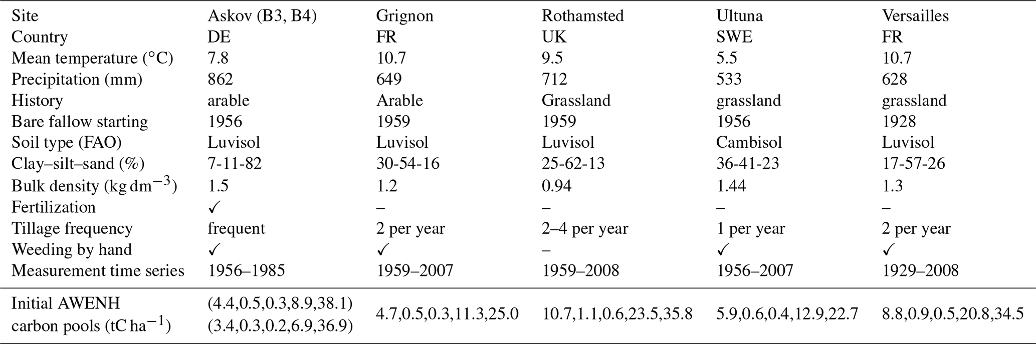
2.2 The measurement time series and the initial carbon pool

Bare fallow experiments included in the study were kept vegetation-free and free of organic amendments for more than 25 years. The study sites are in Europe, and selected characteristics of these are presented in Table 1. The cultivation time that led up to the bare fallow experiment varied from 75 years to centuries. All the SOC measurements are of the bulk soil C without details on AWEN fractions. The sites and the experimental setup are introduced in detail in Barré et al. (2010), Barré et al. (2018) and Menichetti et al. (2019). The detailed setup in Versailles is described also by van Oort et al. (2018) and in Askov by Christensen (1990) and Christensen and Johnston (1997).

Figure 1 Conceptual figure on how the initial states for the model runs are approximated.

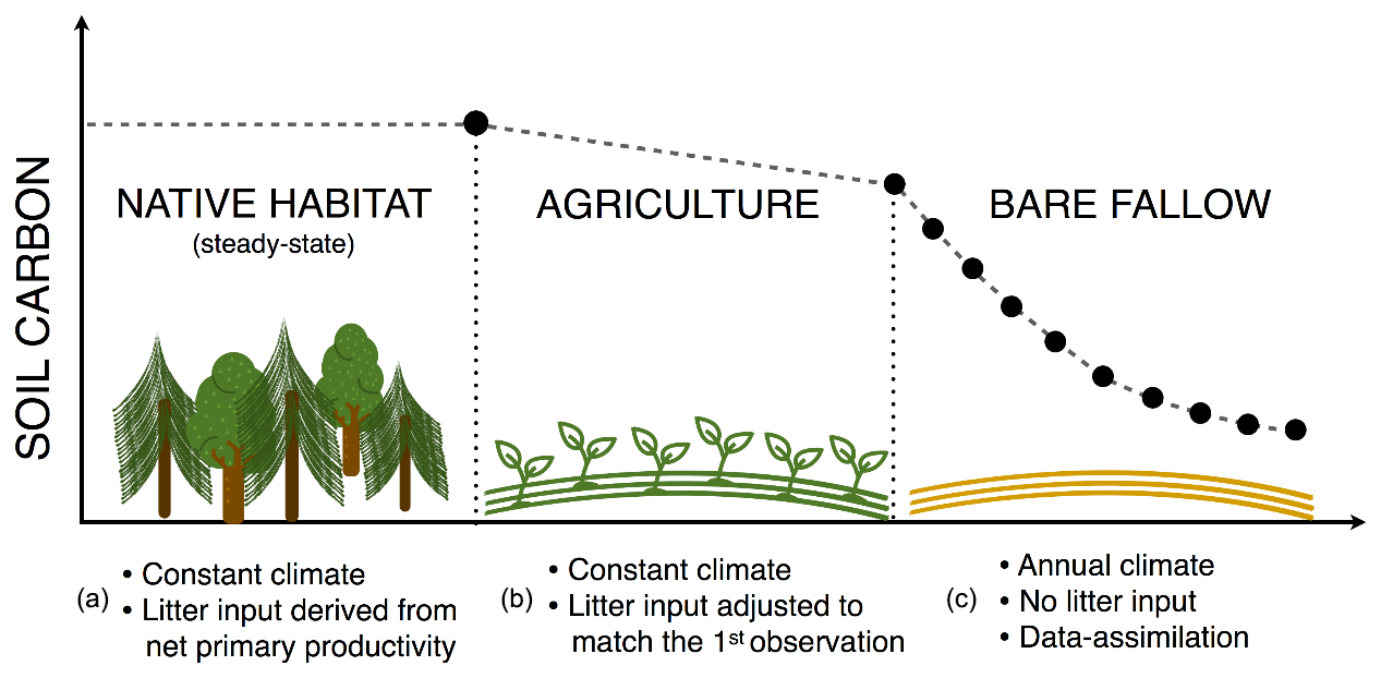
Yasso model requires information on the initial AWENH fractions which we estimated specifically for each site based on the net primary production (NPP) in the presumable native habitat and the estimated litter input during time of cultivation (Fig. 1; Table 1; Kulmala and Liski, 2018). In short, we first made a general NPP estimate in the native habitat using mean temperature and precipitation as in Del Grosso et al. (2008) and divided it into non-woody, small-sized woody and large woody litter fractions based on the native ecosystem. The different litter types had individual carbon fractions based on solubility. Next, we used Yasso to determine the steady-state pool of soil carbon and its fractions using the NPP, different litter fractions, their chemical fractions, and mean temperature and precipitation as driver data (Fig. 1a).

Before bare fallow, each field had been cultivated for 75–300 years. For that period, we simulated SOC starting from the steady-state SOC and its chemical fractions achieved using the pre-agriculture litter approximating (Fig. 1b). The same mean annual temperature and precipitation were used as drivers for both the pre-agriculture and agriculture SOC decomposition. The annual litter input for the cultivation period was estimated in a site-specific manner to meet the first SOC measurement after the cultivation period. The carbon fractions in that litter input were assumed to be as presented in Karhu et al. (2012), and the litter is assumed to be non-woody with a diameter of 0 cm. The resulting SOC is the starting point for the bare fallow period (Fig. 1c). The AWENH distributions calculated in this manner for each site are shown in Table 1 and are used to calculate the z^f from Eq. (4) for the first assimilation cycle as detailed below.

2.3 State data assimilation method

As there is no way to know the true state of a variable, all our information on it, be it modeled or observed, will be inherently uncertain (van Oijen, 2017). State data assimilation (SDA) is a Bayesian statistical method which combines information from multiple sources to create a statistically optimal state estimate. At each assimilation step, SDA updates a priori knowledge of the system state, almost always a model prediction, with state observations. This results in a posterior state estimate of both the expected value and the associated uncertainty. The posterior state estimate is considered the most reliable view on the true state given the available information in model predictions and state observations, thus being less uncertain than all the information sources used to estimate it. Each information source influences the posterior estimate in proportion to their uncertainties: higher observational uncertainty results in a posterior state estimate closer to the model prediction and vice versa (Dietze, 2017).

In our research we used the EAKF (Andersson, 2001), which is based on the Kalman filter theory (Kalman, 1960). The ensemble consists of numerous model projections started from different initial conditions which are moved forward in time independently until the next observation, and the prior state uncertainty is determined from the ensemble spread. At the time of each observation, an update (later called as analysis) is calculated with the following equation:

$$\begin{array}{}\text{(3)}& {\mathit{z}}_i^{\mathrm{a}}={\mathbf{A}}^T\left({\mathit{z}}_i^{\mathrm{f}}-{\stackrel{\mathrm{´}}{\mathit{z}}}^{\mathrm{f}}\right)+{\stackrel{\mathrm{´}}{\mathit{z}}}^{\mathrm{a}},\end{array}$$

where z is a joint state-observation vector, index f denotes forecast, index a denotes analysis and index i denotes each individual ensemble member. Matrix A shifts the whole ensemble so that the updated ensemble has a mean equal to

$$\begin{array}{}\text{(4)}& \overline{{\mathit{z}}^{\mathrm{a}}}={\mathbf{P}}^{\mathrm{a}}\left[({\mathbf{P}}^{\mathrm{f}}{)}^{-\mathrm{1}}\overline{{\mathit{z}}^{\mathrm{f}}}+{\mathbf{H}}^T{\mathbf{R}}^{-\mathrm{1}}\mathit{y}\right]\end{array}$$

and covariance equal to

$$\begin{array}{}\text{(5)}& {\mathbf{P}}^{\mathrm{a}}={\left[({\mathbf{P}}^{\mathrm{f}}{)}^{-\mathrm{1}}+{\mathbf{H}}^T{\mathbf{R}}^{-\mathrm{1}}\mathbf{H}\right]}^{-\mathrm{1}},\end{array}$$

where y is the observation vector, H denotes the observation operator, P is the model state error covariance matrix and R is the observation error covariance. In ensemble Kalman filter applications, each component $P_{ij}^{\mathrm{f}}$ of the forecast error covariance matrix P^f is calculated over the ensemble members

$$\begin{array}{}\text{(6)}& P_{ij}^{\mathrm{f}}={\displaystyle \frac{\sum _{k=\mathrm{1}}^L({\mathit{z}}_{i,k}^{\mathrm{f}}-\overline{{\mathit{z}}_i^{\mathrm{f}}})({\mathit{z}}_{j,k}^{\mathrm{f}}-\overline{{\mathit{z}}_j^{\mathrm{f}}})}{L-\mathrm{1}}},\end{array}$$

where L is the size of the ensemble. It should be noted that the non-diagonal terms of the analysis error covariance matrix P^a represent the error covariances and allow the observation of a specific state also to affect other members of the state variable vector.

There are practical challenges that need to be accounted for when utilizing SDA methods, filter divergence (Schlee et al., 1967) being the most relevant one regarding this study. In practice, the ensemble uncertainty does not represent all the uncertainty sources affecting the model predictions. For example, process error arises due to underrepresented model processes or insufficiently included model interactions. As there are no reliable ways to establish it for process-based simulators like Yasso (van Oijen, 2017), it cannot be accounted for in the assimilation process. Consequently, the modeled uncertainty does not necessarily increase enough to balance out the reduction in posterior uncertainty during the analysis phase. As a result, the updating process gives too much weight to the prior state in comparison to the observed state as the projected uncertainty decreases while the observation uncertainty remains similar. Ultimately a stage is reached where the measurements stop affecting the estimate due to the difference in uncertainties. When this happens, the forecast begins to diverge from reality. There are several methods for dealing with filter divergence (Evensen, 2004; Anderson, 2006), but as this a preliminary study, we used a simple inflation method established in Hamill et al. (2001). In this approach, the forecast/prior covariance is multiplied with a constant factor greater than 1 before every analysis/update step to ensure that the measurement continues to affect the estimate. The practical implementation is explained in more detail in the following section.

2.4 Simulation details

The ensemble initial states were created with R language using the rnorm function with a condition checking that the outputs are non-negative. The initial ensemble values for each pool were determined by drawing from a normal distribution where the initial value for that site was used as a mean. A 10 % mean was used as the initial ensemble variance as there was no reliable initial state uncertainty approximation. This was found to be larger than just perturbing the litter inputs and, as such, was not likely to underestimate the initial uncertainty. For this initial study covariances between the different SOC pools were not considered. The sampling was used to create an ensemble with 50 different states. This way we can represent the uncertainty in the total amount of soil organic carbon and how it is distributed among the five pools. The initial distributions for total carbon are shown in Fig. 2.

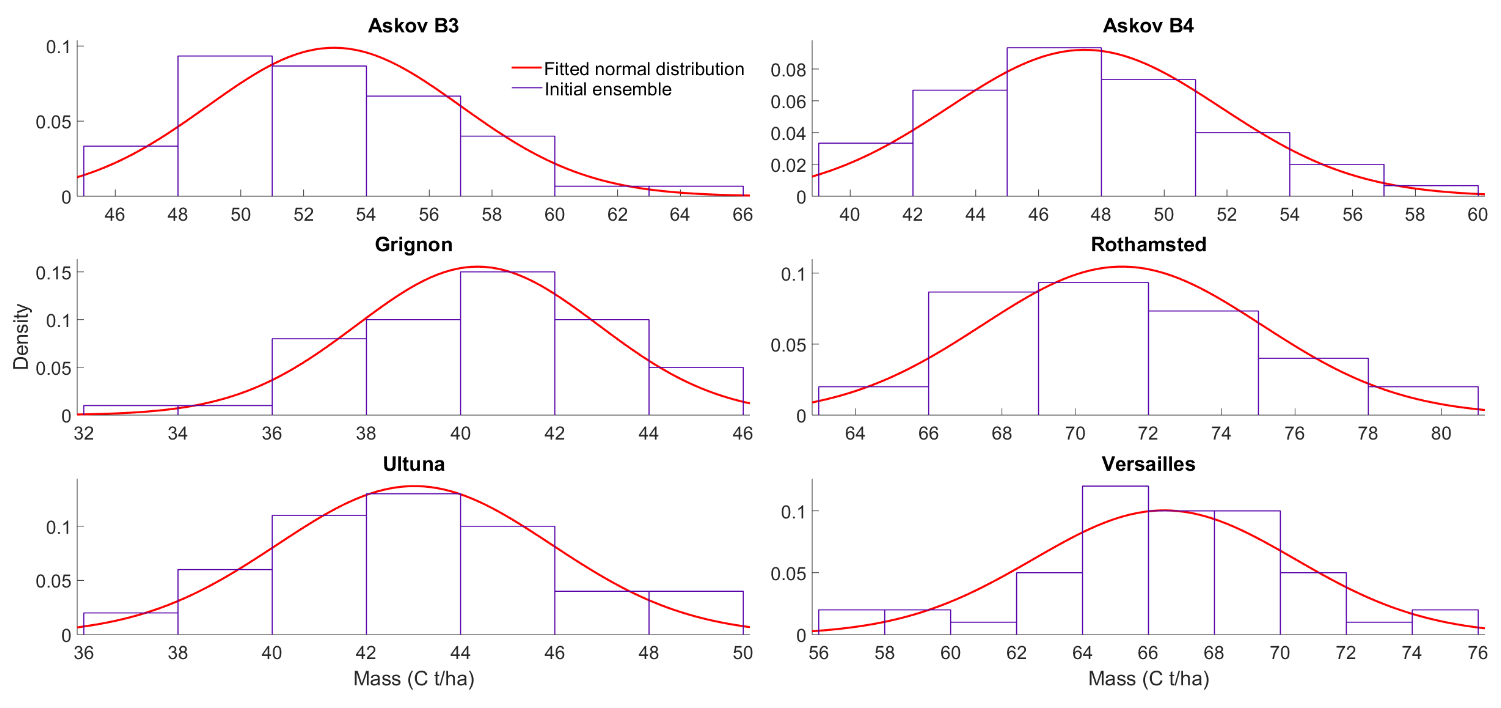
Figure 2 The initial ensemble states of total soil carbon (t ha⁻¹) at the study sites in the beginning of the fallow campaign.

Using the first measurement to scale the initial SOC results in the first measurement to be used twice if the whole measurement time series is used in the SDA implementation. However, not scaling the initial state with the first measurement would cause large differences between the initial state and the first measurement, with the resulting SDA estimations expected to be clearly superior to the non-SDA predictions in such a situation. In other words, it would not be a fair comparison, as generally in runs like these the initial state would be constrained to some degree by available measurements. Another option could be to exclude the first observations from data assimilation. However, including the information from the first measurement in a decomposition time series in the SDA implementation is assumed to be important as the SOC state changes most drastically over the first few years, which in turn would impact the initial state uncertainty propagation. In an ideal situation, there would be an independent SOC measurement that can be used to constrain the SOC initial state, but such additional data were not available here. Thus, we used the whole time series in the assimilation here as using the first measurement twice was expected to have only a very negligible effect on the overall results. We also did a comparison run where the SDA was only applied from the second measurement forward in order to be certain. These runs were set up identically except for the relative error of the first measurement was used as variance to randomly draw the ensemble members.

We used the Data Assimilation Research Testbed (DART; Anderson et al., 2009) to run our assimilation with the EAKF. The initial ensemble for each site was given to DART as a starting point, and climate data measured at the sites were used as model drivers. The climate driver data are provided alongside this article. The state vector consists of the five SOC pool stocks as presented in Yasso and the total SOC, which is a sum of the five pools. The total SOC projection is compared to the measurements, and the error covariances calculated by DART transfer the information to the other state vector components.

The SDA was first tested by updating the model state variables at each measurement time according to Eq. (4), and the produced state estimation was then used by Yasso to determine the next predicted state. This basic test was repeated with three different inflation factors (1, 1.25 and 1.5) in order to examine how much filter divergence affects the projections and which inflation factor range produces satisfactory predictions. The inflation factors were implemented by scaling the posterior error covariance matrix produced by Eq. (6) according to the inflation factor chosen before using it in Eq. (5) and, consequently, in Eq. (4). Only the inflation factor results for 1.0 and 1.25 are shown here for the sake of clarity. In the second set of tests, only a limited number of initial measurements (first, first two, first three or first four) are used to update the state before it is then allowed to run the whole time series freely without being updated with measurement information to determine how soon the measurement information begins to noticeably impact the model projections. Only the first four measurements were used in this phase as the central question was how assimilating SOC measurements impact long-term forecasts. The inflation factor of 1.25 was used in these latter tests.

All the forecasts produced with these tests were compared to both measurements and baseline Yasso SOC projection that was run from the initial state without any SDA. In order to better assess how the SDA improved the state forecasts, we calculated the RMSE for the last four measurements at each site for all the five experiments: the baseline Yasso model forecast, SDA with first observation only, SDA with the first two, and the first three and first four observations using the forecasts that used the limited number of measurements as well as the baseline Yasso model forecast.

3 Results

Using SOC data to update the state of the model improved the model-calculated estimates compared to non-SDA model projections run from the approximated initial state (Fig. 2). While the inflated SDA predictions (inflation factor 1.25) had larger uncertainties than the uninflated ones (inflation factor 1.0), the predictions themselves remained close to each other with the exception of the two Askov sites. There, systematic shifts occur in the observed states decades after the start of the time series, and indicative of the effect of the filter divergence, the uninflated SDA predictions did not react to these shifts while the inflated SDA predictions were adjusted to the new states. Applying the inflation value of 1.5, the analysis essentially matched the measurements (Fig. S1 in the Supplement).

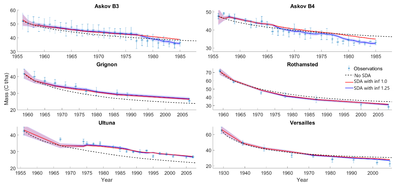
Figure 3 Observed and modeled SOC with and without data assimilation (SDA) of all previous measurements using two different inflation factors (inf). The colored area around the two different SDA estimates indicates the 95 % confidence interval. SDA with a higher inflation factor improved predictions at all sites, while the SDA with a lower inflation factor was susceptible to filter divergence.

Due to the multiple changes in the Askov B4 time series, the more detailed model state response is represented for it to see how the state estimate adapts to the changes there. Among the SOC pools, the humus pool changed most in response to the observations and always to their direction at Askov B4 (Fig. 3). The SDA estimate affected the AWEN pools only a little during the first half of the time series, but after approximately 10 years, these pools were also changed during the state update. Interestingly, these pools were changed to the opposite direction compared to the humus pool and observations. SDA affected the humus pool in a same way at other sites, and a similar difference in the behavior between the AWEN and the humus pools was observed at Askov B3 after the systematic shift (Figs. S2–S6).

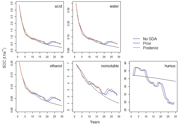
Figure 4 The mean of prior and posterior distribution SOC pools at Askov B4 before and after each assimilated observation. Different SOC pools showed different responses to SDA where humus pool was adjusted the most in response to the observations and always to their direction. AWEN pool dynamics responded SDA later over the course of assimilation.

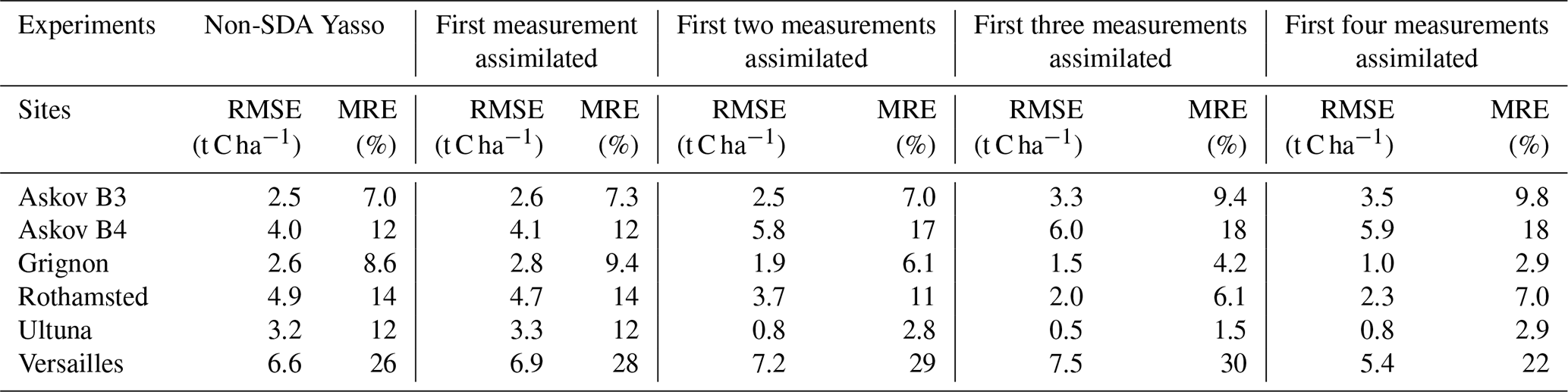
At most sites incorporating information already from the first two observations had a noticeable impact on the time series prediction. However, at the Versailles site, the SDA forecast was close to the non-SDA forecasts at the end of the time series (Fig. 4). At the Askov sites, the updated predictions ended up overestimating the latest measurements more than the model alone did due to the systematic shift in measurement values (at Askov B4 after 1966 and at Askov B3 after 1977). Finally, RMSE values (Table 2) show that aside from Askov, the assimilation reduced the RMSE at each site by the fourth measurement at the latest.

Table 2 The root mean square error (RMSE) as well as the mean relative error (MRE) respective to the observation for the three last measurement at each site. The unit for the RMSE values is tonnes of carbon per hectare.

The comparison runs where the assimilation was only done from the second measurement forward were nearly identical for the estimated total SOC values when continuously assimilating and when only using the first few observations to constrain the predictions (figures not shown). The more detailed examination of the state at Askov B4 (Fig. 5) did show a difference, as the later corrections affecting the AWEN pools are more muted than if the assimilation begun from the first measurement of the time series.

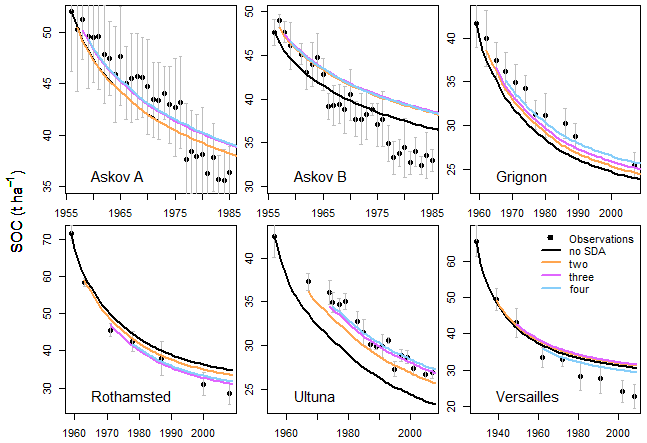
Figure 5 Observed and forecasted SOC without data assimilation (black) and with 2–4 initial observations assimilated (colored lines). Incorporating information already from the first two observations had a noticeable impact on the time series prediction.

4 Discussion

This study establishes that state data assimilation (SDA) improves soil organic carbon (SOC) forecasts by continuously incorporating total carbon measurements. As such, this adds another type of measurements that SDA can use to improve future projections in addition to previously shown positive impacts of assimilating soil environmental conditions (Yan et al., 2019). At all sites assimilating already the first few measurements had a clear impact on the forecasts (Fig. 4; Table 2). It should be noted that at Askov, the non-SDA forecast is closer to the measurements towards the end of the time series than the SDA forecast that assimilated the first few observations. This is due to the systematic shift in measured SOC that happens at Askov B3 around 1965 and at Askov B4 around 1975. Before that, the SDA forecasts are closer to the SOC measurements than the non-SDA forecasts. This supports previous research on the impact of initial state uncertainty on SOC projections (Todd-Brown et al., 2014; He et al., 2016).

While the inflation term does increase the uncertainty of the forecasts and thus reduces the filter divergence, the uninflated and inflated forecasts remain similar. Askov sites are the exception here as there the inflated SDA forecast reacts to the previously noted systematic shift in measurement time series. This is expected as the inflation reduces the impact of filter divergence and thus allows for the later observations to affect the analysis more than they would without the uncertainty inflation. These results here indicate that it succeeds in the framework discussed in Anderson (2001) on how inflated systems should behave. However, once litter input will be introduced into the system, it will add a potentially systematic source of error as the uncertainties in the litter input affect the SOC projections. At that point, a more nuanced inflation approach or other more elaborate implementations, such as estimating the process variance from observations (Dietze, 2017), could be required.

When examining how SDA affects the model state, it is important to note that the total SOC measurements affect the model state based on the error covariances between the different pools and their total SOC. The initial uncertainties were introduced as independent of each other with the SDA calculating the error covariances between the different pools over the analysis process. The resulting error covariance between the humus pool and total SOC is strongly positive with a decrease in humus also decreasing total SOC and vice versa (Fig. 4). This is reasonable as the long-lived SOC is generally dominated by the stable humus pool (Lehmann and Kleber, 2015), and adjusting to it is crucial in capturing the decomposition without litter input. Furthermore, due to the slow decomposition rate of the H pool and the relatively high frequency of the observations, in Fig. 4 the prior H value is essentially the posterior H of the previous assimilation cycle.

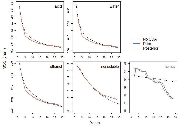
Figure 6 The mean prior and posterior distribution SOC pools at Askov B4 before and after each assimilated observation if the assimilation begins from the second observation. While the AWEN pools still show an opposite shift to the H pool later in the assimilation cycle, it is smaller than in Fig. 3.

Error covariances between the AWEN pools and total SOC are more complicated than between SOC and H pool. Thus, it takes more analysis cycles for the method to establish them. Consequently, the analysis appears to affect the humus SOC from the start of the time series while with AWEN pools the analysis impact appears to become stronger later into the time series. Due to this, the two Askov time series are the only sites where we also capture the meaningful AWEN pool impacts due to the late shift in the observed state. Even there, though, covariance is strongly affected if the uncertainty spread over the first few years of the decomposition is included (Figs. 4 and 6). It is noteworthy that once the SDA properly determines the error covariance structures, the analysis adjusts the AWEN pools to the opposite direction compared to the H pool. Initially, this might appear to be counterintuitive, as SDA increases the AWEN values in response for the forecast overestimating the SOC values, but this is due to model dynamics being reflected via the error covariances. Further complicating the matter is that the active AWEN pools are affected differently by the environmental conditions compared to the inactive H pools (Tuomi et al., 2008). This will cause the resulting AWENH error covariances to vary between locations even if the total carbon and H error covariance appears to be consistent.

In addition to providing a valuable illustration of how the error covariances change over time and impact the later state corrections, the Askov sites also highlight both a strength and limitation of the SDA methods. As seen in the measurement time series (Fig. 3), both Askov B3 and B4 have a systematic shift in measurements at different times due to reasons currently not known. The model projections alone cannot capture these developments as it is unclear whether the sudden drop in observed SOC is even due to an ecological process not represented in the model or some issues relating to the measurements. In either case, the inflated SDA adapts to the new state within a few measurement cycles and produces a forecast that follows the new state well. This is clearly a strength of the SDA method that would be beneficial when forecasting SOC at locations where there are disturbances and alterations in the surface conditions. However, here the new state estimate appears questionable as there is a sudden increase in active SOC (i.e., AWEN pools) despite it being over a decade since there was any litterfall. This goes against the current understanding of the system as there is no transference from the H pool back to the AWEN pools and no litter to provide those faster decomposing carbon compounds. In this case, the late increases of the AWEN pool concentrations at the Askov sites are an artifact of the error covariances established earlier rather than a realistic representation of what is happening in the soil. Thus, while SDA is a beneficial tool when examining changing systems, the nature of SOC model dynamics makes it important to also expertly assess how the new estimated state reacts to those changes.

Another site that shows SDA having challenges is Versailles, where SDA only slightly improves the forecasts towards the end of the time series. This is probably due to either the model not representing a SOC decomposition dynamic relevant to that particular site, or the input drivers are somehow lacking. This site highlights that while SDA is a valuable tool for improving forecasts, it is still limited by how well the applied model captures the local SOC dynamics. For instance, if the soil respiration parameters for the H pool is poorly represented for that location, then the resulting H pool, as well as the total SOC, projections would still be more uncertain even when applying SDA methods (Gao et al., 2011). However, SDA is still useful in these situations as it can indicate sites where the forecast error is not driven by the state uncertainty. Therefore, it is easier to analyze the differences between the sites like Ultuna and Versailles. For example, it is known that soil quality affects the SOC decomposition (Chapin et al., 2011; Vogel et al., 2015), so here it would support further research on the soil properties at Versailles to determine whether those dynamics have an impact there that should be acknowledged with SOC forecasts at other similar sites.

The continuous SDA forecasts from Askov sites and Versailles (Fig. 3) also indicate the complexity of the filter divergence issue in SOC systems and how it should be accounted for. As explained in Sect. 2.2, one of the key reasons for filter divergence is due to the prior state uncertainty being underestimated due to ignoring of model process error, which results in the prior state being given progressively more and more weight in the assimilation phase. At more frequently measured sites, such as Askov B3 and B4, there are more assimilation steps, which would intuitively speed up the filter divergence issue. However, as can be seen in Eq. (6), the reduction in posterior uncertainty depends on the observation uncertainty, with less uncertain observations also reducing the posterior uncertainty more. Thus, at the Askov site, the measurement uncertainties are large enough that it partially balances out the measurement frequency, and the resulting forecast uncertainty is large enough to allow for rapid adaptation to changes in the system.

At Versailles, though, while the measurements are much less frequent, they also have small associated uncertainties, especially the first few ones. Furthermore, for long decomposition systems like this, the uncertainty propagation within the ensemble is so slow that it only marginally increases the state uncertainty until the next observation point, resulting in filter divergence becoming an even more pronounced issue here. As a result, even with uncertainty inflation, the first few assimilation steps reduce the state uncertainties to the degree that the difference between projections and measurements affects the state estimate much less than at the other sites. The new observations still affected the inflated SDA, as can be seen at the last Versailles measurement in Fig. 3, but it will take multiple observations with increasing difference between forecasted and measured state for SDA to properly adjust to the new state. This highlights the importance of carefully considering the relationships between the observation uncertainty, frequency and inflation in order to improve the assimilation results. This is also a general issue within the application of SDA in geosciences and, as such, there have already been attempts to mathematically address it (e.g., Li et al., 2009).

5 Conclusion

The results here show that there are benefits in implementing SDA methods in SOC research as assimilating the first few observations was generally sufficient in improving long-term SOC projections when compared to later measurements. Furthermore, the SDA methods here successfully used coarse bulk C measurements to update the more detailed model state with the developing error covariance matrices connecting the different state variables. The work also highlights the need for additional study such as, for example, how to best address the filter divergence issue or what is driving the differences in how SDA performs at different sites. The focus here was on a very simple system where there was no litter input and on a specific SDA method with its own benefits and hindrances. Increasing the complexity of the system, such as by introducing different types of litter, using measurements from other locations to estimate local SOC or incorporating flux tower respiration measurements to constrain projected SOC changes, will raise new practical challenges that have to be addressed in future work. Still, by allowing actively incorporating multiple information sources, SDA is a crucial tool for all process-based model projections, for example approximating the amount of SOC in a forest or assessing how agricultural carbon allocation changes in response to field management.