Extending square conservation to arbitrarily structured C-grids with shallow water equations

The square conservation law is implemented in atmospheric dynamic cores on latitude–longitude grids, but it is rarely implemented on quasi-uniform grids, given the difficulty involved in constructing anti-symmetrical spatial discrete operators on these grids. Increasingly more models are being developed on quasi-uniform grids, such as arbitrarily structured C-grids. Thuburn–Ringler–Skamarock–Klemp (TRiSK) is a shallow water dynamic core on an arbitrarily structured C-grid. The spatial discrete operator of TRiSK is able to naturally maintain the conservation properties of total mass and total absolute vorticity and conserving total energy with time truncation error; the first two integral invariants are exactly conserved during integration, but the total energy dissipates when using the dissipative temporal integration schemes, i.e., Runge–Kutta (RK). The method of strictly conserving the total energy simultaneously, which means conserving energy in the round-off error over the entire temporal integration period, uses both an anti-symmetrical spatial discrete operator and a square conservative temporal integration scheme. In this study, we demonstrate that square conservation is equivalent to energy conservation in both a continuous shallow water system and a discrete shallow water system of TRiSK. After that, we attempt to extend the square conservation law to the TRiSK framework. To overcome the challenge of constructing an anti-symmetrical spatial discrete operator, we unify the unit of evolution variables of shallow water equations using the Institute of Atmospheric Physics (IAP) transformation, and the temporal derivatives of new evolution variables can be expressed by a combination of temporal derivatives of original evolution variables, which means the square conservative spatial discrete operator can be obtain by using original spatial discrete operators in TRiSK. Using the square conservative Runge–Kutta scheme, the total energy is completely conserved, and there is no influence on the properties of conserving total mass and total absolute vorticity. In the standard shallow water numerical test, the square conservative scheme not only helps maintain total conservation of the three integral invariants but also creates less simulation error norms.

1 Introduction

In a statistical sense, the integral constraints make the physics of the discrete model more analogous to the physics of the continuous atmosphere, and also make the errors less systematic (Arakawa and Lam, 1977). Shallow water equation sets, without any outer sources and frictions, have five basic physical conservation properties, including total mass, total energy, total absolute vorticity (total potential vorticity), total potential enstrophy and total angular momentum. These conservation properties are important in an atmosphere model, especially with regard to long-term simulation; however, in a discrete system, some conservation properties cannot be maintained (Wang, 2008). If the square of a quantity is conserved with time when summed up over all the grid points in a domain, the quantity itself will be bounded, at every individual grid point, throughout the entire period of integration; this might be helpful for preventing nonlinear computational instability (Arakawa, 1966), and energy is one kind of quadratic quantity. Toy and Nair (2017) developed an energy and potential enstrophy conserving scheme for shallow water equations on generalized curvilinear coordinates; they mentioned conserving analogues of total energy, and total potential enstrophy in numerical models is known to prevent a spurious cascade of energy toward small scales. For a short-term simulation, the influences of slight energy dissipation are not obvious, but this dissipation accumulates in every time step, and finally, in a long-term simulation, leads to a quiet different result; i.e., an ellipse orbit tends to a single point after 10⁸ steps (Wang et al., 1996).

A numerical scheme, with an energy conservation or energy dissipative property, is prerequisite to prevent nonlinear computational instability; however, an energy dissipative scheme will limit short waves, which are meaningful for the atmosphere (Shen et al., 2015; Zeng and Ji, 1981). On a latitude–longitude grid, energy can be entirely conserved by constructing a square conservative finite-difference scheme (Ji and Wang, 1991) or a multi-conservation finite-difference scheme (Wang and Ji, 2003), the former being better developed. Wang and Ji (1994a) discussed the square conservative scheme (SCS), the complete square conservative scheme (CSCS), the instantaneous square conservative scheme (ISCS) and the explicit complete square conservative scheme with adjustable time intervals (ECSCSA). The ISCS maintains square conservation only in the spatial discrete scheme and not in the temporal integration scheme, which implies that the spatial discrete operator of the model is a square conservative (i.e., an anti-symmetrical operator). However, the temporal integration scheme does not possess the square conservation property; therefore, the model is energy dissipative during integration. The CSCS maintains square conservation in both the spatial and temporal schemes. The model, which adopts CSCS, is able to maintain complete energy conservation during integration. The first step of applying the square conservation theory is to construct an anti-symmetrical spatial discrete operator, and the second step is to integrate the model with a square conservative temporal integration scheme, e.g., a modified predictor–corrector, modified leap-frog (Wang and Ji, 2006), harmonious dissipative operators (Wang and Ji, 1994b), etc.

To improve integration precision on the temporal direction of the square conservative scheme, a new class of new Runge–Kutta (NRK) schemes were developed by Wang et al. (1996). The NRK scheme maintains the complete square conservation property by adjusting the length of temporal integration steps and maintaining the same integral precision order as the original Runge–Kutta (RK) scheme.

The SCS was implemented in the grid-point atmospheric model of IAP LASG (GAMIL, Wang et al., 2004; Wang and Ji, 2006). GAMIL is widely used in climate simulation (Li et al., 2007, 2013; Wu and Li, 2008). The square conservation theory is rarely used on quasi-uniform grids or nonuniform grids because it is hard to construct a spatial discrete operator with an anti-symmetrical property on those grids.

In the past 2 decades, to avoid the polar singularity of the latitude–longitude grid, increasingly more atmosphere models have been built on the quasi-uniform grid, e.g., spectral transform methods (Swarztrauber, 1996), the finite-volume method (Lin, 2004; Putman and Lin, 2007; Chen and Xiao, 2008) and an extension of the finite-difference method to the generalized curvilinear coordinates (Toy and Nair, 2017).

Thuburn et al. (2009) and Ringler et al. (2010) provided a spatial discrete scheme based on arbitrarily structured C-grids, known as Thuburn–Ringler–Skamarock–Klemp (TRiSK). TRiSK is able to conserve total mass and total absolute vorticity, and total energy is conserved within time truncation error. These important properties allow for models using quasi-uniform Voronoi grids, the accuracies of which are similar to latitude–longitude grids (Weller et al., 2012). Based on Thuburn et al. (2009) and Ringler et al. (2010), a global/regional model, the Model for Prediction Across Scales (MPAS), was developed by the National Center for Atmospheric Research (NCAR) and Los Alamos National Laboratory (LANL; Skamarock et al., 2012, 2018).

Although the spatial discrete operator designed by Ringler et al. (2010) results in energy conservation, the total energy is still dissipative while using dissipative temporal integration schemes, i.e., Runge–Kutta; in other words, the conservation property of spatial discrete operator is not able to be maintain during temporal integration, which is referred to as conserving total energy in time truncation error. In this paper we attempt to construct a square conservative scheme for TRiSK, which is able to conserve total energy in the round-off error, but not just in time truncation error; this means that the variation of total energy should be in the round-off error during the entire temporal integration period. We call this complete energy conservation.

Total energy will be completely conserved only if the spatial discrete operator is anti-symmetrical and the temporal integration scheme is square conservative (Wang and Ji, 2006). The main obstacle of extending square conservation to the quasi-uniform grids is constructing the anti-symmetrical spatial discrete operator. Because many quasi-uniform grids are unstructured and the shapes of cells are not uniform, it is difficult to find the next or previous cell. In this study, we use the instantaneous energy conservation property of TRiSK to overcome the challenge of constructing an anti-symmetrical spatial operator on a quasi-uniform grid. After using NRK as a temporal integration scheme, the square conservative constraints are satisfied for both spatial and temporal directions, and the total energy, total mass and total absolute vorticity are completely conserved during the integration.

This paper is presented as follows: in Sect. 2, we review the TRiSK framework described by Ringler et al. (2010). Section 3 describes the method of extending square conservation to TRiSK in three parts. The first part presents a review of square conservation and a demonstration of the equivalent relationship between square conservation and energy conservation in a continuous shallow water system. In the second part of Sect. 3, we obtain the anti-symmetrical spatial discrete operator by using the derivative rule and the energy conservation property of TRiSK, a method that is key to extending square conservation to TRiSK. In the last part of Sect. 3, we review a new type of Runge–Kutta with fourth-order precision, which was developed by Wang et al. (1996), as the square conservative temporal integration scheme. In Sect. 4, by using the square conservation scheme, we demonstrate that the total mass and total absolute vorticity remain perfectly conservative. Section 5 exhibits the results of three different numerical tests, including the second, fifth and sixth test cases mentioned by Williamson et al. (1992).

2 Introduction of TRiSK

The shallow water equation set may be written in a vector-invariant form as follows:

$$\begin{array}{}\text{(1)}& {\displaystyle }& {\displaystyle \frac{\partial \mathit{u}}{\partial t}}-{\mathit{\xi }}_{\mathrm{a}}\mathit{k}\times \mathit{u}+\mathrm{\nabla }E=\mathrm{0},\text{(2)}& {\displaystyle }& {\displaystyle \frac{\partial \mathit{\varphi }}{\partial t}}+\mathrm{\nabla }\cdot \left(\mathit{\varphi }\mathit{u}\right)=\mathrm{0},\end{array}$$

where ${\mathit{\xi }}_{\mathrm{a}}=\mathit{\xi }+f$ denotes the absolute vorticity; $\mathit{\xi }=\mathrm{\nabla }\times \mathit{u}$ represents the relative vorticity; f=2Ωsin θ is the Coriolis parameter; $E=K+g(h+h_{\mathrm{s}})=K+\mathit{\varphi }+{\mathit{\varphi }}_{\mathrm{s}}$, ϕ=gh is the geopotential depth of the fluid; ϕ_s=gh_s is the geopotential height of the underlying surface; ${\mathit{\varphi }}_{\mathrm{t}}=\mathit{\varphi }+{\mathit{\varphi }}_{\mathrm{s}}$ is the free surface (top) of the fluid; $K=\frac{|\mathit{u}{|}^{\mathrm{2}}}{\mathrm{2}}$ is the kinetic energy; u is the velocity vector; h and h_s are the fluid thickness and surface height, respectively; θ represents the latitude; and g and Ω are acceleration of gravity and angular velocity of the earth.

In Ringler et al. (2010), the total energy is defined as

$$\begin{array}{}\text{(3)}& {\mathit{ϵ}}_{\mathrm{R}\mathrm{10}}=hK+gh\left({\displaystyle \frac{\mathrm{1}}{\mathrm{2}}}h+h_{\mathrm{s}}\right).\end{array}$$

To simplify the derivation in the following context, we define the total energy as

$$\begin{array}{}\text{(4)}& \begin{array}{rl}\underset{\mathrm{\Omega }}{∯}\mathit{ϵ}\mathrm{d}s& =\underset{\mathrm{\Omega }}{∯}g{\mathit{ϵ}}_{\mathrm{R}\mathrm{10}}\mathrm{d}s=\underset{\mathrm{\Omega }}{∯}\mathit{\varphi }K+{\displaystyle \frac{\mathrm{1}}{\mathrm{2}}}{\mathit{\varphi }}^{\mathrm{2}}+\mathit{\varphi }{\mathit{\varphi }}_{\mathrm{s}}\mathrm{d}s\\ & =\Vert \mathit{\varphi }K\Vert +∥{\displaystyle \frac{\mathrm{1}}{\mathrm{2}}}{\mathit{\varphi }}^{\mathrm{2}}∥+∥\mathit{\varphi }{\mathit{\varphi }}_{\mathrm{s}}∥,\end{array}\end{array}$$

where $\Vert \cdot \Vert =\sqrt{(\cdot ,\cdot )}$ denotes the 2-norm. The inner product ($\cdot ,\cdot$) is defined as

$$\begin{array}{}\text{(5)}& (X,Y)=\underset{\mathrm{\Omega }}{∯}X\cdot Y\mathrm{d}s,\end{array}$$

where Ω is the entire spherical surface.

Per the description provided in Ringler et al. (2010), velocity points are on the edges of each cell, the mass and kinetic energy points are in the center of each cell and vorticity points are on the vertices of each cell. The shallow water equation set may be expressed as a discrete form:

$$\begin{array}{}\text{(6)}& {\displaystyle }& {\displaystyle \frac{\partial u_e}{\partial t}}-Q_e^{\perp }+[\mathrm{\nabla }E{]}_e=\mathrm{0},\text{(7)}& {\displaystyle }& {\displaystyle \frac{\partial {\mathit{\varphi }}_i}{\partial t}}+[\mathrm{\nabla }\cdot (\mathit{\varphi }u){]}_i=\mathrm{0},\end{array}$$

where u_e, ϕ_i are the normal velocity and geopotential height. The subscript “e” signifies that the variable is defined on edge e; the subscript i signifies that the variable is defined at the center of ith cell. $Q_e^{\perp }$ is the absolute vorticity flux on the tangent direction ⊥ of the edge e, which is computed according to Eq. (49) in Ringler et al. (2010). Another two functions in Eqs. (6) and (7) are given by the introduction of Fig. 3 in Ringler et al. (2010):

$$\begin{array}{}\text{(8)}& {\displaystyle }& {\displaystyle }[\mathrm{\nabla }E{]}_e={\displaystyle \frac{\mathrm{1}}{d_e}}\sum _{i\in \mathrm{CE}\left(e\right)}-n_{e,i}{E}_i,\text{(9)}& {\displaystyle }& {\displaystyle }[\mathrm{\nabla }\cdot (\mathit{\varphi }u){]}_i={\displaystyle \frac{\mathrm{1}}{A_i}}\sum _{e\in \mathrm{EC}\left(i\right)}{n}_{e,i}{l}_e{\mathit{\varphi }}_e{u}_e,\end{array}$$

where n_e,i is an indicator function, defined as $n_{e,i}=\mathrm{1}$ when n_e is an outward normal vector of cell i, and $n_{e,i}=-\mathrm{1}$ when n_e is an inward normal vector of cell i; l_e is the length of edge e; i∈CE(e) denotes the two cells that share edge e; and e∈EC(i) is the set of edges that define the boundary of cell i. The potential vorticity on edge q_e may be computed by the midpoint method (Ringler et al., 2010, Eq. 50) or the linear interpolation method (Weller, 2012, Eq. 5). The details are presented in Fig. 1.

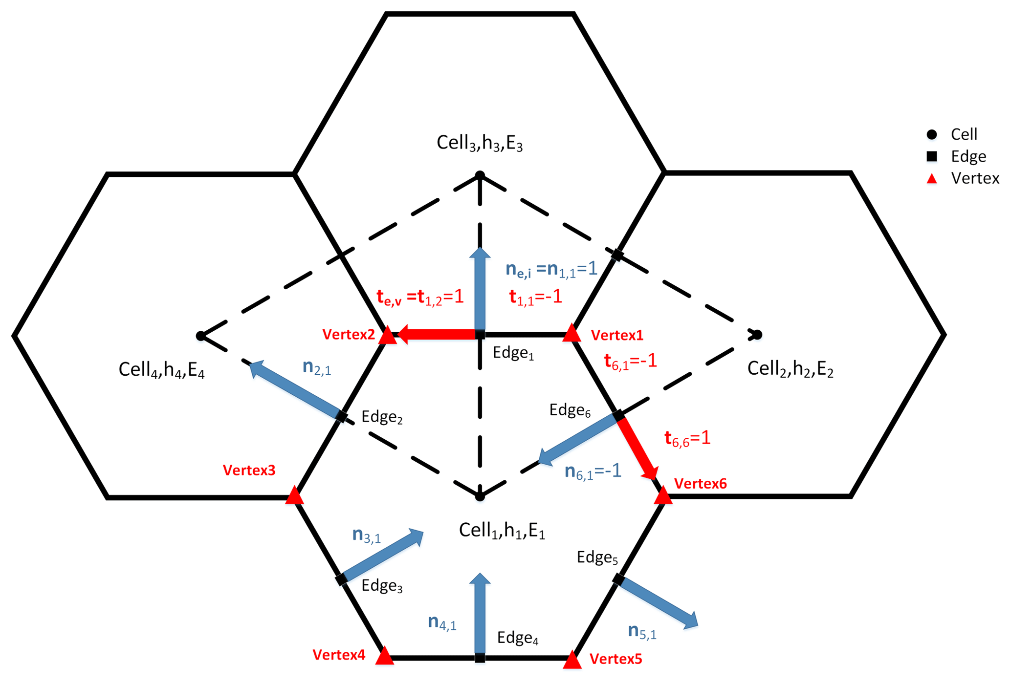
Figure 1 Definition of elements in a discrete system. Blue arrows represent the indicator function n_e,i and red arrows are the indicator function t_e,v. The uniform grid is here for clearly introducing SCVT meshes, the situation on non-uniform grid is similar.

3 Extending the square conservation to TRiSK

As mentioned in Sect. 1, to obtain the complete square conservation property, the spatial discrete operator must be anti-symmetrical, and the temporal integration scheme is square conservative. Therefore, in this section, the method of extending the square conservation to TRiSK is introduced in three parts. Section 3.1 reviews the concept of square conservation, demonstrating the equivalent relationship between the square conservation and energy conservation. Section 3.2 constructs the anti-symmetrical spatial discrete operator. Section 3.3 introduces the square conservative temporal integration scheme by reviewing a class of NRK, developed by Wang et al. (1996).

3.1 Relationship between square conservation and energy conservation

First, we review the concept of anti-symmetrical operators and square conservation according to the study of Wang et al. (1996), considering the nonlinear evolution equation in operator form:

$$\begin{array}{}\text{(10)}& {\displaystyle \frac{\partial \mathit{F}}{\partial t}}+\mathcal{L}\left(\mathit{F}\right)=\mathrm{0}.\end{array}$$

Definition. Suppose H is a complete inner product space on R and ℒ is an H→H operator; if ℒ satisfies the following inner product equation

$$\begin{array}{}\text{(11)}& \left(\mathcal{L}\right(\mathit{F}),\mathit{F})=\mathrm{0},\end{array}$$

then ℒ is termed an anti-symmetrical operator.

The result of multiplying F on both sides of Eq. (10) and integrating globally is the square conservation property:

$$\begin{array}{}\text{(12)}& {\displaystyle \frac{\mathrm{d}}{\mathrm{d}t}}\Vert \mathit{F}{\Vert }^{\mathrm{2}}=\mathrm{0}.\end{array}$$

Next, we begin determining the relationship between energy conservation and square conservation. In the TRiSK framework, the evolution variables are u and ϕ.

The unified unit of evolution variables is the prerequisite of constructing the square conservation system. The evolution variables are unified by IAP transformation (Zeng and Zhang, 1987; Wang et al., 2004), and the original evolution variable u is replaced by the new evolution variable $\mathit{U}=\sqrt{\mathit{\varphi }}\mathit{u}$, after completing IAP transformation.

$$\begin{array}{}\text{(13)}& \mathit{F}=\left(\begin{array}{l}\mathit{U}\\ \mathit{\varphi }\end{array}\right)=\left(\begin{array}{l}\sqrt{\mathit{\varphi }}\mathit{u}\\ \mathit{\varphi }\end{array}\right).\end{array}$$

The physical significance of $\sqrt{\mathit{\varphi }}$ is the phase speed of the external gravity wave, and the shallow water equation set may be rewritten as a vector format:

$$\begin{array}{}\text{(14)}& {\displaystyle \frac{\partial \mathit{F}}{\partial t}}+\mathcal{L}\left(\mathit{F}\right)={\displaystyle \frac{\partial }{\partial t}}\left(\begin{array}{l}\mathit{U}\\ \mathit{\varphi }\end{array}\right)+\mathcal{L}\left(\begin{array}{l}\mathit{U}\\ \mathit{\varphi }\end{array}\right)=\mathrm{0}.\end{array}$$

As defined in Sect. 2, ${\mathit{\varphi }}_{\mathrm{t}}=\mathit{\varphi }+{\mathit{\varphi }}_{\mathrm{s}}$, and

$$\begin{array}{}\text{(15)}& {\displaystyle \frac{\partial {\mathit{\varphi }}_{\mathrm{t}}}{\partial t}}={\displaystyle \frac{\partial \mathit{\varphi }}{\partial t}}+{\displaystyle \frac{\partial {\mathit{\varphi }}_{\mathrm{s}}}{\partial t}}.\end{array}$$

The surface height is determined to be independent of time,

$$\begin{array}{}\text{(16)}& {\displaystyle \frac{\partial {\mathit{\varphi }}_{\mathrm{s}}}{\partial t}}=\mathrm{0}.\end{array}$$

Therefore,

$$\begin{array}{}\text{(17)}& {\displaystyle \frac{\partial {\mathit{\varphi }}_{\mathrm{t}}}{\partial t}}={\displaystyle \frac{\partial \mathit{\varphi }}{\partial t}}.\end{array}$$

Defining ${\mathit{F}}_{\mathrm{t}}=\left(\begin{array}{l}\mathit{U}\\ {\mathit{\varphi }}_{\mathrm{t}}\end{array}\right)$, according to Eqs. (13) and (17), we have

$$\begin{array}{}\text{(18)}& {\displaystyle \frac{\partial {\mathit{F}}_{\mathrm{t}}}{\partial t}}={\displaystyle \frac{\partial \mathit{F}}{\partial t}}.\end{array}$$

Multiplying Eq. (18) by F_t on both sides, and integrating globally, we have

$$\begin{array}{}\text{(19)}& \begin{array}{rl}{\displaystyle \frac{\mathrm{d}}{\mathrm{d}t}}∥{\displaystyle \frac{\mathrm{1}}{\mathrm{2}}}{\mathit{F}}_{\mathrm{t}}^{\mathrm{2}}∥& =\left(F_{\mathrm{t}},{\displaystyle \frac{\partial \mathit{F}}{\partial t}}\right)=\underset{\mathrm{\Omega }}{∯}\mathit{U}{\displaystyle \frac{\partial \mathit{U}}{\partial t}}+\left(\mathit{\varphi }+{\mathit{\varphi }}_{\mathrm{s}}\right){\displaystyle \frac{\partial \mathit{\varphi }}{\partial t}}\mathrm{d}s\\ & =\underset{\mathrm{\Omega }}{∯}{\displaystyle \frac{\partial }{\partial t}}\left({\displaystyle \frac{\mathrm{1}}{\mathrm{2}}}|\mathit{U}{|}^{\mathrm{2}}\right)+{\displaystyle \frac{\partial }{\partial t}}\left({\displaystyle \frac{\mathrm{1}}{\mathrm{2}}}{\mathit{\varphi }}^{\mathrm{2}}+\mathit{\varphi }{\mathit{\varphi }}_{\mathrm{s}}\right)\mathrm{d}s\\ & ={\displaystyle \frac{\mathrm{d}}{\mathrm{d}t}}\left(\Vert \mathit{\varphi }K\Vert +∥{\displaystyle \frac{\mathrm{1}}{\mathrm{2}}}{\mathit{\varphi }}^{\mathrm{2}}∥+∥\mathit{\varphi }{\mathit{\varphi }}_{\mathrm{s}}∥\right)={\displaystyle \frac{\mathrm{d}\mathit{ϵ}}{\mathrm{d}t}}=\mathrm{0}.\end{array}\end{array}$$

Accordingly, square conservation is equivalent to energy conservation in a continuous system.

3.2 Constructing the anti-symmetrical spatial discrete operator

In this subsection, we construct the anti-symmetrical spatial discrete operator using a specific combination of original operators in TRiSK. Firstly, we need to demonstrate the equivalent relationship between the square conservative spatial discrete operator and energy conservative spatial discrete operator in a continuous system; then we prove that this relationship is also applicable to discrete system.

Assuming a continuous-in-time system, the evolution equation of U is able to be expressed as

$$\begin{array}{}\text{(20)}& {\displaystyle \frac{\partial \mathit{U}}{\partial t}}=\sqrt{\mathit{\varphi }}{\displaystyle \frac{\partial \mathit{u}}{\partial t}}+{\displaystyle \frac{\mathit{u}}{\mathrm{2}\sqrt{\mathit{\varphi }}}}{\displaystyle \frac{\partial \mathit{\varphi }}{\partial t}}.\end{array}$$

This formula is key to connecting square conservation and energy conservation; in the following theorem, we obtain an anti-symmetrical operator by using Eq. (20).

Theorem. The functions $\mathcal{M}=\mathcal{M}(\mathit{\varphi },u)$ and $\mathcal{N}=\mathcal{N}(\mathit{\varphi },u)$ satisfy

$$\begin{array}{}\text{(21)}& \left\{\begin{array}{l}\frac{\partial \mathit{u}}{\partial t}+\mathcal{M}=\mathrm{0}\\ \frac{\partial \mathit{\varphi }}{\partial t}+\mathcal{N}=\mathrm{0}\end{array}\right.,\end{array}$$

and

$$\begin{array}{}\text{(22)}& (\mathcal{M},\mathit{\varphi }u)+(\mathcal{N},E)=\mathrm{0}.\end{array}$$

After IAP transformation Eq. (13), the evolution equation of U may be expressed as Eq. (20). Meanwhile, Eq. (21) may be rewritten as Eq. (14).

If the operator ℒ satisfies Eq. (14), then ℒ is an anti-symmetrical operator.

Proof.

$$\begin{array}{}\text{(23)}& {\displaystyle \frac{\partial \mathit{U}}{\partial t}}=\sqrt{\mathit{\varphi }}{\displaystyle \frac{\partial \mathit{u}}{\partial t}}+{\displaystyle \frac{\mathit{u}}{\mathrm{2}\sqrt{\mathit{\varphi }}}}{\displaystyle \frac{\partial \mathit{\varphi }}{\partial t}}=-\sqrt{\mathit{\varphi }}\mathcal{M}-{\displaystyle \frac{\mathit{u}}{\mathrm{2}\sqrt{\mathit{\varphi }}}}\mathcal{N},\end{array}$$

$$\begin{array}{}\text{(24)}& \begin{array}{rl}\left(\mathcal{L}\right(\mathit{F}),\mathit{F})& =-\left({\displaystyle \frac{\partial \mathit{U}}{\partial t}},\mathit{U}\right)-\left({\displaystyle \frac{\partial \mathit{\varphi }}{\partial t}},\mathit{\varphi }\right)\\ & =\underset{\mathrm{\Omega }}{∯}-\mathit{U}{\displaystyle \frac{\partial \mathit{U}}{\partial t}}-\mathit{\varphi }{\displaystyle \frac{\partial \mathit{\varphi }}{\partial t}}\mathrm{d}s\\ & =\underset{\mathrm{\Omega }}{∯}-\mathit{U}\left(-\sqrt{\mathit{\varphi }}\mathcal{M}-{\displaystyle \frac{\mathit{u}}{\mathrm{2}\sqrt{\mathit{\varphi }}}}\mathcal{N}\right)+\mathit{\varphi }\mathcal{N}\mathrm{d}s\\ & =\underset{\mathrm{\Omega }}{∯}\mathit{\varphi }\mathit{u}\cdot \mathcal{M}+{\displaystyle \frac{|\mathit{u}{|}^{\mathrm{2}}}{\mathrm{2}}}\mathcal{N}+\mathit{\varphi }\mathcal{N}\mathrm{d}s\\ & =(\mathcal{M},\mathit{\varphi }\mathit{u})+(\mathcal{N},E)=\mathrm{0}.\end{array}\end{array}$$

This theorem is proved in a continuous system, but the model is built as a discrete system; therefore, it is necessary to discuss the situation in a discrete space.

Following Ringler et al. (2010), we define the functions M=M(ϕ, u) and N=N(ϕ, u) in discrete space as follows:

$$\begin{array}{}\text{(25)}& {\displaystyle }& {\displaystyle }M=[\mathrm{\nabla }E{]}_e-Q_e^{\perp },\text{(26)}& {\displaystyle }& {\displaystyle }N=[\mathrm{\nabla }\cdot (\mathit{\varphi }u){]}_i.\end{array}$$

And the semi-discrete shallow water equation set becomes

$$\begin{array}{}\text{(27)}& {\displaystyle }& {\displaystyle \frac{\partial u}{\partial t}}+M=\mathrm{0},\text{(28)}& {\displaystyle }& {\displaystyle \frac{\partial \mathit{\varphi }}{\partial t}}+N=\mathrm{0}.\end{array}$$

Because the spatial discrete operator of TRiSK has an instantaneous energy conservation property, it is easy to prove $(M,\mathit{\varphi }u)+(N,E)=\mathrm{0}$ (details in Sect. 3.7.2 of Ringler et al., 2010).

There are cells, edges and vertices presented as three types of points on a spherical centroidal Voronoi tessellation (SCVT) grid, which is the mesh used by TRiSK. We define the inner product for different types of points as follows:

$$\begin{array}{}\text{(29)}& {\displaystyle }& {\displaystyle }(X,Y{)}_i=\sum _{i=\mathrm{1}}^{\mathrm{nCells}}{X}_i\cdot Y_i\cdot A_i,\text{(30)}& {\displaystyle }& {\displaystyle }(X,Y{)}_e=\sum _{e=\mathrm{1}}^{\mathrm{nEdges}}{X}_e\cdot Y_e\cdot A_e,\end{array}$$

where X_iY_i are the variables in the cell; X_eY_e denote any variables on the edge; A_iA_e are the areas for each cell and edge; $A_e=d_e\times l_e$, d_e is the distance between the two cells' centers on edge e; l_e is the length of edge e; “nCells” denotes the total cell number; and “nEdges” is the total edge number.

$$\begin{array}{}\text{(31)}& (M,\mathit{\varphi }u{)}_e+(N,E{)}_i=\mathrm{0}.\end{array}$$

Combining Eqs. (14) and (20), and rewriting it into a discrete system:

$$\begin{array}{}\text{(32)}& {\displaystyle \frac{\partial \mathit{F}}{\partial t}}+L\left(\mathit{F}\right)={\displaystyle \frac{\partial }{\partial t}}\left(\begin{array}{l}{U}_e\\ {\mathit{\varphi }}_i\end{array}\right)+L\left(\begin{array}{l}{U}_e\\ {\mathit{\varphi }}_i\end{array}\right)=\mathrm{0},\end{array}$$

where $U_e=\sqrt{{\mathit{\varphi }}_e}{u}_e$, $\sqrt{{\mathit{\varphi }}_e}$ is the phase speed of external gravity wave on edge e. Note that we need to interpolate ϕ_i from cell center i to edge e; here we set ${\mathit{\varphi }}_e=\frac{\mathrm{1}}{\mathrm{2}}\sum _{i\in \mathrm{CE}\left(e\right)}{\mathit{\varphi }}_i$.

$$\begin{array}{}\text{(33)}& {\displaystyle \frac{\partial U_e}{\partial t}}=\sqrt{{\mathit{\varphi }}_e}{\displaystyle \frac{\partial u_e}{\partial t}}+{\displaystyle \frac{u_e}{\mathrm{2}{\sqrt{\mathit{\varphi }}}_e}}{\displaystyle \frac{\partial {\mathit{\varphi }}_e}{\partial t}}=-\sqrt{{\mathit{\varphi }}_e}M-{\displaystyle \frac{u_e}{\mathrm{2}{\sqrt{\mathit{\varphi }}}_e}}N.\end{array}$$

As shown in Appendix A, we have the discrete anti-symmetrical operator L:

$$\begin{array}{}\text{(34)}& \left(L\right(\mathit{F}),\mathit{F}{)}_{\mathrm{d}}=-{\left(U,{\displaystyle \frac{\partial U}{\partial t}}\right)}_e-{\left(\mathit{\varphi },{\displaystyle \frac{\partial \mathit{\varphi }}{\partial t}}\right)}_i=\mathrm{0}.\end{array}$$

The subscript “d” represents that the inner product is computed in a discrete system.

Thus, the discrete evolution equation set becomes

$$\begin{array}{}\text{(35)}& {\displaystyle }& {\displaystyle \frac{\partial U_e}{\partial t}}+\sqrt{{\mathit{\varphi }}_e}M+{\displaystyle \frac{u_e}{\mathrm{2}\sqrt{{\mathit{\varphi }}_e}}}N=\mathrm{0},\text{(36)}& {\displaystyle }& {\displaystyle \frac{\partial {\mathit{\varphi }}_i}{\partial t}}+N=\mathrm{0}.\end{array}$$

The model will be instantaneous square conservative by incorporating Eqs. (35) and (36) as the evolution equation set.

3.3 Constructing the temporal integration scheme with the square conservation property

The model is integrated in a discrete-in-time system; for the sake of guaranteeing complete square conservation, a square conservative temporal integration scheme is necessary. As NRK has the advantage of maintaining complete square conservation with a high order of integral precision, the fourth-order NRK scheme in TRiSK is adopted to obtain high integral precision and a long time step. To completely introduce the square conservative temporal integration scheme, we review some details of Wang et al. (1996).

The fourth-order NRK may be expressed as

$$\begin{array}{}\text{(37)}& {\mathit{F}}^{n+\mathrm{1}}={\mathit{F}}^n+{\mathit{\tau }}_n\mathit{\phi }\left({\mathit{F}}^n,\mathit{\tau }\right),\end{array}$$

where τ_n is an adjustable time step and τ is the integral time step of the model.

$$\begin{array}{}\text{(38)}& {\displaystyle }& {\displaystyle }\mathit{\phi }\left({\mathit{F}}^n,\mathit{\tau }\right)=\mathit{\tau }{\displaystyle \frac{{\mathit{R}}_{\mathrm{1}}+\mathrm{2}{\mathit{R}}_{\mathrm{2}}+\mathrm{2}{\mathit{R}}_{\mathrm{3}}+{\mathit{R}}_{\mathrm{4}}}{\mathrm{6}}}.\text{(39)}& {\displaystyle }& {\displaystyle }\left\{\begin{array}{l}{\mathit{R}}_{\mathrm{1}}=-L{\mathit{F}}^n\\ {\mathit{R}}_{\mathrm{2}}=-L\left({\mathit{F}}^n+\frac{\mathrm{1}}{\mathrm{2}}\mathit{\tau }{\mathit{R}}_{\mathrm{1}}\right)\\ {\mathit{R}}_{\mathrm{3}}=-L\left({\mathit{F}}^n+\frac{\mathrm{1}}{\mathrm{2}}\mathit{\tau }{\mathit{R}}_{\mathrm{2}}\right)\\ {\mathit{R}}_{\mathrm{4}}=-L\left({\mathit{F}}^n+\mathit{\tau }{\mathit{R}}_{\mathrm{3}}\right).\end{array}\right.\end{array}$$

Taking square operators on both sides of Eq. (37), delineating ${\mathit{\phi }}^n=\mathit{\phi }({\mathit{F}}^n,\mathit{\tau })$,

$$\begin{array}{}\text{(40)}& {∥{\mathit{F}}^{n+\mathrm{1}}∥}^{\mathrm{2}}={∥{\mathit{F}}^n∥}^{\mathrm{2}}+\mathrm{2}{\mathit{\tau }}_n\left({\mathit{\phi }}^n,{\mathit{F}}^n\right)+{\mathit{\tau }}_n^{\mathrm{2}}{∥{\mathit{\phi }}^n∥}^{\mathrm{2}}.\end{array}$$

We note that although the spatial discrete operator L is anti-symmetrical, the total energy at the n+1 time point remains different from that at the n time point. Energy is able to be completely conserved by satisfying the following equation:

$$\begin{array}{}\text{(41)}& {∥{\mathit{F}}^{n+\mathrm{1}}∥}^{\mathrm{2}}={∥{\mathit{F}}^n∥}^{\mathrm{2}}.\end{array}$$

Therefore,

$$\begin{array}{}\text{(42)}& {\displaystyle }& {\displaystyle }\mathrm{2}{\mathit{\tau }}_n\left({\mathit{\phi }}^n,{\mathit{F}}^n\right)+{\mathit{\tau }}_n^{\mathrm{2}}{∥{\mathit{\phi }}^n∥}^{\mathrm{2}}=\mathrm{0},\text{(43)}& {\displaystyle }& {\displaystyle }{\mathit{\tau }}_n=-{\displaystyle \frac{\mathrm{2}\left({\mathit{\phi }}^n,{\mathit{F}}^n\right)}{{∥{\mathit{\phi }}^n∥}^{\mathrm{2}}}}.\end{array}$$

Considering the situation when τ→0, and according to Eqs. (17) and (18) in Wang et al. (1996),

$$\begin{array}{}\text{(44)}& {\mathit{\tau }}_n={\displaystyle \frac{\mathit{\tau }}{\mathrm{3}{∥{\mathit{\phi }}^n∥}^{\mathrm{2}}}}\left[\left({\mathit{R}}_{\mathrm{1}},{\mathit{R}}_{\mathrm{2}}\right)+\left({\mathit{R}}_{\mathrm{2}},{\mathit{R}}_{\mathrm{3}}\right)+\left({\mathit{R}}_{\mathrm{3}},{\mathit{R}}_{\mathrm{4}}\right)\right].\end{array}$$

Once adopting the NRK scheme as the temporal integration scheme, the model will be completely square conservative, which implies that the total energy will be completely conserved from the beginning to the end of the integration. The NRK scheme is expected to perform better than RK in a numerical test. Moreover, NRK decays to RK by setting τ_n=τ.

While the integral time step is modified from τ to τ_n, the precision order of NRK is the same as RK; when constructing NRK based on the nth order RK, NRK has nth order precision as well, a conclusion proven by Theorem 1 in Wang et al. (1996).

4 Mass and absolute vorticity conservation

In the CSCS introduced above, although the integral time step is modified from τ to τ_n, total mass and total absolute vorticity are nevertheless conserved. In the following demonstrations, we note that the mass conservation property and absolute vorticity conservation property are independent of temporal integration.

4.1 Mass conservation

Considering the total mass, multiplying Eq. (7) by A_i and summing all cells,

$$\begin{array}{}\text{(45)}& \begin{array}{rl}\sum _{i=\mathrm{1}}^{\mathrm{nCells}}{A}_i{\displaystyle \frac{\partial {\mathit{\varphi }}_i}{\partial t}}& =-\sum _{i=\mathrm{1}}^{\mathrm{nCells}}{A}_i[\mathrm{\nabla }\cdot (\mathit{\varphi }u){]}_i\\ & =-\sum _{i=\mathrm{1}}^{\mathrm{nCells}}\sum _{e\in \mathrm{EC}\left(i\right)}{n}_{e,i}{l}_e{\mathit{\varphi }}_e{u}_e\\ & =-\sum _{e=\mathrm{1}}^{\mathrm{nEdges}}\sum _{i\in \mathrm{CE}\left(e\right)}{n}_{e,i}{l}_e{\mathit{\varphi }}_e{u}_e\\ & =-\sum _{e=\mathrm{1}}^{\mathrm{nEdges}}{l}_e{\mathit{\varphi }}_e{u}_e-l_e{\mathit{\varphi }}_e{u}_e=\mathrm{0}.\end{array}\end{array}$$

Note that the mass conservation property is independent of temporal integration.

4.2 Absolute vorticity conservation

According to Eq. (23) in Ringler et al. (2010), the relative vorticity is calculated according to the following diagnostic equation:

$$\begin{array}{}\text{(46)}& \mathit{\xi }={\displaystyle \frac{\mathrm{1}}{A_v}}\sum _{e\in \mathrm{EV}\left(v\right)}{t}_{e,v}{u}_e{d}_e.\end{array}$$

Multiplying by A_v and summing all of the vertices yields

$$\begin{array}{}\text{(47)}& \begin{array}{rl}\sum _{v=\mathrm{1}}^{\mathrm{nVertices}}{A}_v\mathit{\xi }& =\sum _{v=\mathrm{1}}^{\mathrm{nVertices}}\sum _{e\in \mathrm{EV}\left(v\right)}{t}_{e,v}{u}_e{d}_e\\ & =\sum _{e=\mathrm{1}}^{\mathrm{nEdges}}\sum _{v\in \mathrm{VE}\left(e\right)}{t}_{e,v}{u}_e{d}_e\\ & =\sum _{e=\mathrm{1}}^{\mathrm{nEdges}}{u}_e{d}_e-u_e{d}_e=\mathrm{0},\end{array}\end{array}$$

where e∈EV(v) represents the set of edges that share the vertex v; v∈VE(e) are the two vertices on edge e. The indicator function t_e,v always points to the left side of n_e,i. If $\mathit{k}\times n_{e,i}$ is directed toward vertex v, then $t_{e,v}=\mathrm{1}$; otherwise, $t_{e,v}=-\mathrm{1}$. k is the unit vector, which points in the local vertical direction. See Fig. 1 for details. The total relative vorticity is shown to always be zero and independent of time.

Another method to compute the relative vorticity is to use the following prognostic equation, as described in Eq. (33) of Ringler et al. (2010):

$$\begin{array}{}\text{(48)}& {\displaystyle \frac{\partial \mathit{\xi }}{\partial t}}+{\displaystyle \frac{\mathrm{1}}{A_v}}\sum _{e\in \mathrm{EV}\left(v\right)}-t_{e,v}{Q}_e^{\perp }{d}_e=\mathrm{0}.\end{array}$$

Multiplying the above equation by A_v and summing all the vertices yields

$$\begin{array}{}\text{(49)}& \begin{array}{rl}\sum _{v=\mathrm{1}}^{\mathrm{nVertices}}{A}_v{\displaystyle \frac{\partial \mathit{\xi }}{\partial t}}& =\sum _{v=\mathrm{1}}^{\mathrm{nVertices}}\sum _{e\in \mathrm{EV}\left(v\right)}{t}_{e,v}{Q}_e^{\perp }{d}_e\\ & =\sum _{e=\mathrm{1}}^{\mathrm{nEdges}}\sum _{v\in \mathrm{VE}\left(e\right)}{t}_{e,v}{Q}_e^{\perp }{d}_e\\ & =\sum _{e=\mathrm{1}}^{\mathrm{nEdges}}{Q}_e^{\perp }{d}_e-Q_e^{\perp }{d}_e=\mathrm{0}.\end{array}\end{array}$$

Therefore, the relative vorticity is conserved during temporal integration.

Taking the partial derivative of the absolute vorticity with time yields

$$\begin{array}{}\text{(50)}& {\displaystyle \frac{\partial {\mathit{\xi }}_{\mathrm{a}}}{\partial t}}={\displaystyle \frac{\partial \mathit{\xi }}{\partial t}}+{\displaystyle \frac{\partial f}{\partial t}}.\end{array}$$

The Coriolis parameter is independent of time, $\frac{\partial f}{\partial t}=\mathrm{0}$; thus

$$\begin{array}{}\text{(51)}& \sum _{v=\mathrm{1}}^{\mathrm{nVertices}}{A}_v{\displaystyle \frac{\partial {\mathit{\xi }}_{\mathrm{a}}}{\partial t}}=\mathrm{0}.\end{array}$$

5 Numerical tests

To test the square conservation schemes using TRiSK, a new TRiSK-based shallow water dynamic core is developed, which is named TRiSK-based Multiple-Conservation dynamical cORE (TMCORE). The spatial discrete operators are the same as those introduced by Ringler et al. (2010), the evolution variable u_e is replaced by U_e, as we described above, and the temporal integration scheme is selected from RK or NRK, both of which are of fourth-order precision.

We expected that the square conservation scheme will work on arbitrarily structured C-grids with a different initial field and mesh of a different resolution. In this section, we test the new scheme by using standard shallow water test cases 2, 5 and 6 (SWTC2, SWTC5, SWTC6) with two different meshes, as presented by Williamson et al. (1992). The first mesh has 2562 Voronoi cells (x1.2562), with an approximate resolution of 480 km, and the second mesh contains 40 962 Voronoi cells (x1.40962), with an approximate resolution of 120 km. The corresponding integral time steps to x1.2562 and x1.40962 are 900 and 360 s. Here, the midpoint scheme is selected as the method for interpolating the potential vorticity from vertices to edges for all tests.

In all of the test cases, we expect the complete energy conservation scheme (NRK) is able to conserve total mass, total absolute vorticity and total energy in the round-off error; meanwhile, it would be even better if NRK could provide us with a lower simulation error. Note, total energy is not merely conserved in time truncation error anymore; we need the change ratio of total energy to be limited to at least 10⁻¹⁴ magnitude.

5.1 Error measure methods

The global invariants error measure is as follows:

$$\begin{array}{}\text{(52)}& I\left(X^n\right)={\displaystyle \frac{S\left(X_i^n\right)-S\left(X_i^{\mathrm{0}}\right)}{S\left(X_i^{\mathrm{0}}\right)}},\end{array}$$

where $X_i^n$ is the variable at the nth time point on the ith cell and $X_i^{\mathrm{0}}$ is the variable at the initial time. The I function is the change ratio of the invariants.

The total mass error measure is as follows:

$$\begin{array}{}\text{(53)}& {\displaystyle }& {\displaystyle }{X}_i^n=h_i^n,\text{(54)}& {\displaystyle }& {\displaystyle }\mathrm{Mass}\mathrm{change}\mathrm{ratio}=I\left(h^n\right).\end{array}$$

The total energy error measure is as follows:

$$\begin{array}{}\text{(55)}& {\displaystyle }& {\displaystyle }{X}_i^n={\mathit{ϵ}}_i^n,\text{(56)}& {\displaystyle }& {\displaystyle }\mathrm{Energy}\mathrm{change}\mathrm{ratio}=I\left({\mathit{ϵ}}^n\right).\end{array}$$

Measuring the fluid thickness error by L₂ and L_∞ error norms is expressed as

$$\begin{array}{}\text{(57)}& {\displaystyle }& {\displaystyle }{L}_{\mathrm{2}}={\displaystyle \frac{{\left\{S\left[{\left(f_{\mathrm{m}}\left(i\right)-f_{\mathrm{R}}\left(i\right)\right)}^{\mathrm{2}}\right]\right\}}^{\frac{\mathrm{1}}{\mathrm{2}}}}{{\left[S\left(f_{\mathrm{R}}(i{)}^{\mathrm{2}}\right)\right]}^{\frac{\mathrm{1}}{\mathrm{2}}}}},\text{(58)}& {\displaystyle }& {\displaystyle }{L}_{\mathrm{\infty }}={\displaystyle \frac{\max \left|f_{\mathrm{m}}\left(i\right)-f_{\mathrm{R}}\left(i\right)\right|}{\max \left|f_{\mathrm{R}}\left(i\right)\right|}},\end{array}$$

where i denotes the index of each cell; f_m(i) and f_R(i), respectively, are the model solution and reference solution at the ith cell on the mesh; and the S function is the area-weighted accumulation of an arbitrary variable X.

$$\begin{array}{}\text{(59)}& S\left(X\right)={\displaystyle \frac{\sum _{i=\mathrm{1}}^{N}X\left(i\right)A\left(i\right)}{\sum _{i=\mathrm{1}}^{N}A\left(i\right)}},\end{array}$$

where A(i) is the area of the ith cell.

The reference solution should be an analytical solution or, when an analytical solution is not available, a high-resolution solution from the model with sufficient accuracy.

In the following context, NRK4 represents the NRK with fourth-order precision and RK4 represents the original Runge–Kutta scheme with fourth-order precision.

The differences of the error norms between NRK4 and RK4 schemes by using the different ratios of L₂ (L2DR) and L_∞ (LInfDR) are expressed as follows:

$$\begin{array}{}\text{(60)}& {\displaystyle }& {\displaystyle }\mathrm{L}\mathrm{2}\mathrm{DR}={\displaystyle \frac{L_{{\mathrm{2}}_{\mathrm{CRK}\mathrm{4}}}-L_{{\mathrm{2}}_{\mathrm{RK}\mathrm{4}}}}{L_{{\mathrm{2}}_{\mathrm{RK}\mathrm{4}}}}},\text{(61)}& {\displaystyle }& {\displaystyle }\mathrm{LInfDR}={\displaystyle \frac{L_{{\mathrm{\infty }}_{\mathrm{CRK}\mathrm{4}}}-L_{{\mathrm{\infty }}_{\mathrm{RK}\mathrm{4}}}}{L_{{\mathrm{\infty }}_{\mathrm{RK}\mathrm{4}}}}},\end{array}$$

where $L_{{\mathrm{2}}_{\mathrm{NRK}\mathrm{4}}}$ and $L_{{\mathrm{2}}_{\mathrm{RK}\mathrm{4}}}$ are the L₂ error norms of NRK4 and RK4, respectively, which is similar for $L_{{\mathrm{\infty }}_{\mathrm{NRK}\mathrm{4}}}$ and $L_{{\mathrm{\infty }}_{\mathrm{RK}\mathrm{4}}}$. NRK4 performs better than RK4 when the different ratios are negative; otherwise, NRK4 performs worse than RK4.

5.2 Global steady-state nonlinear zonal geostrophic flow (SWTC2)

For the global steady-state nonlinear zonal geostrophic flow test case, the initial velocity field has the following form

$$\begin{array}{}\text{(62)}& {\displaystyle }& {\displaystyle }u=u_{\mathrm{0}}\cos \mathit{\theta },\text{(63)}& {\displaystyle }& {\displaystyle }v=\mathrm{0}.\end{array}$$

The geopotential height field is

$$\begin{array}{}\text{(64)}& \mathrm{gh}={\mathrm{gh}}_{\mathrm{0}}-\left(a\mathrm{\Omega }{u}_{\mathrm{0}}+{\displaystyle \frac{u_{\mathrm{0}}^{\mathrm{2}}}{\mathrm{2}}}\right){\sin }^{\mathrm{2}}\mathit{\theta }.\end{array}$$

Here, we set $\mathrm{\Omega }=\mathrm{7.292}\times {\mathrm{10}}^{-\mathrm{5}}$ s⁻¹, g=9.80616 m s⁻², $a=\mathrm{6.37122}\times {\mathrm{10}}^{\mathrm{6}}$ m, gh${}_{\mathrm{0}}=\mathrm{2.94}\times {\mathrm{10}}^{\mathrm{4}}$ m² s⁻² and $u_{\mathrm{0}}=\mathrm{2}\mathit{\pi }a/$(12 d), where h is fluid thickness and θ denotes latitude. In this test case, the exact solution is the initial state, and any difference between the numerical solution and the initial state is the simulation error.

In SWTC2, the true solution of $\frac{\partial u}{\partial t}$, $\frac{\partial v}{\partial t}$, $\frac{\partial \mathit{\varphi }}{\partial t}$ is always zero; therefore, this test case can only represent the precision of spatial discrete operators but not the precision of temporal integration. This simulation is integrated for 10 years, but the shape of geostrophic flow breaks after 7 years. Therefore, we choose the simulation results from the first to the seventh year to compare the error norms of NRK4 and RK4.

Figure 2 measures the L₂ and L_∞ error norms of geopotential height. In the first 4 years, the NRK4 and RK4 exhibit similar results, but in the last 3 years, the shape of geopotential flow tends to break. The error norms increase sharply after 6 years, and the differences between NRK4 and RK4 become more evident. Both the L₂ and L_∞ error norms of NRK4 are evidently smaller than RK4, and the collapse of geopotential flow is delayed approximately 1 month when using NRK4.

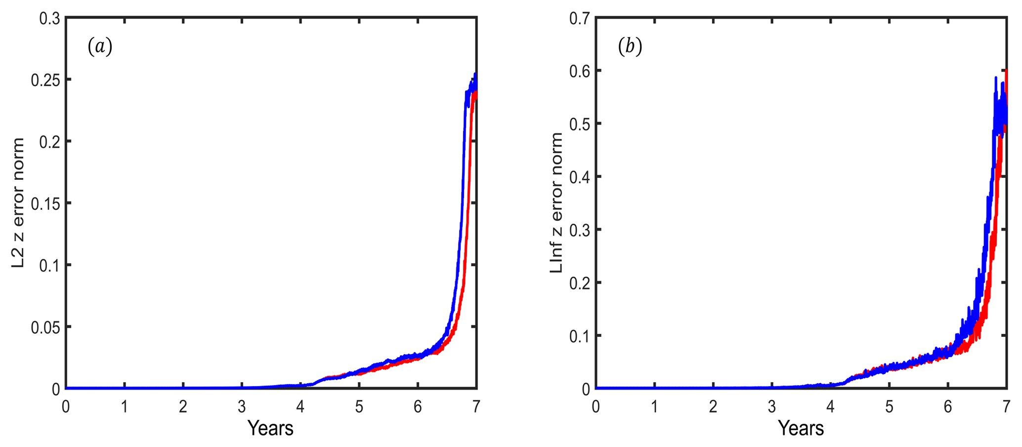
Figure 2 Geopotential height error norms of SWTC2. (a) L₂ error norm; (b) L_∞ error norm. The results of RK4 and NRK4 are represented by blue and red lines, respectively. The model mesh is x1.2562.

Figure 3 presents the variation of invariants as a function of time. The change ratio of total mass is limited to 10⁻¹⁵ magnitude, and total absolute vorticity oscillates around 10⁻²⁰ magnitude, which means these two invariants are strictly conserved. The total energy of RK4 decreased approximately 0.5 % in the final year, but NRK4 maintains strict energy conservation (at 10⁻¹⁵ magnitude). Although the geopotential flow has been broken, NRK4 prevents an increasing rate of total potential enstrophy.

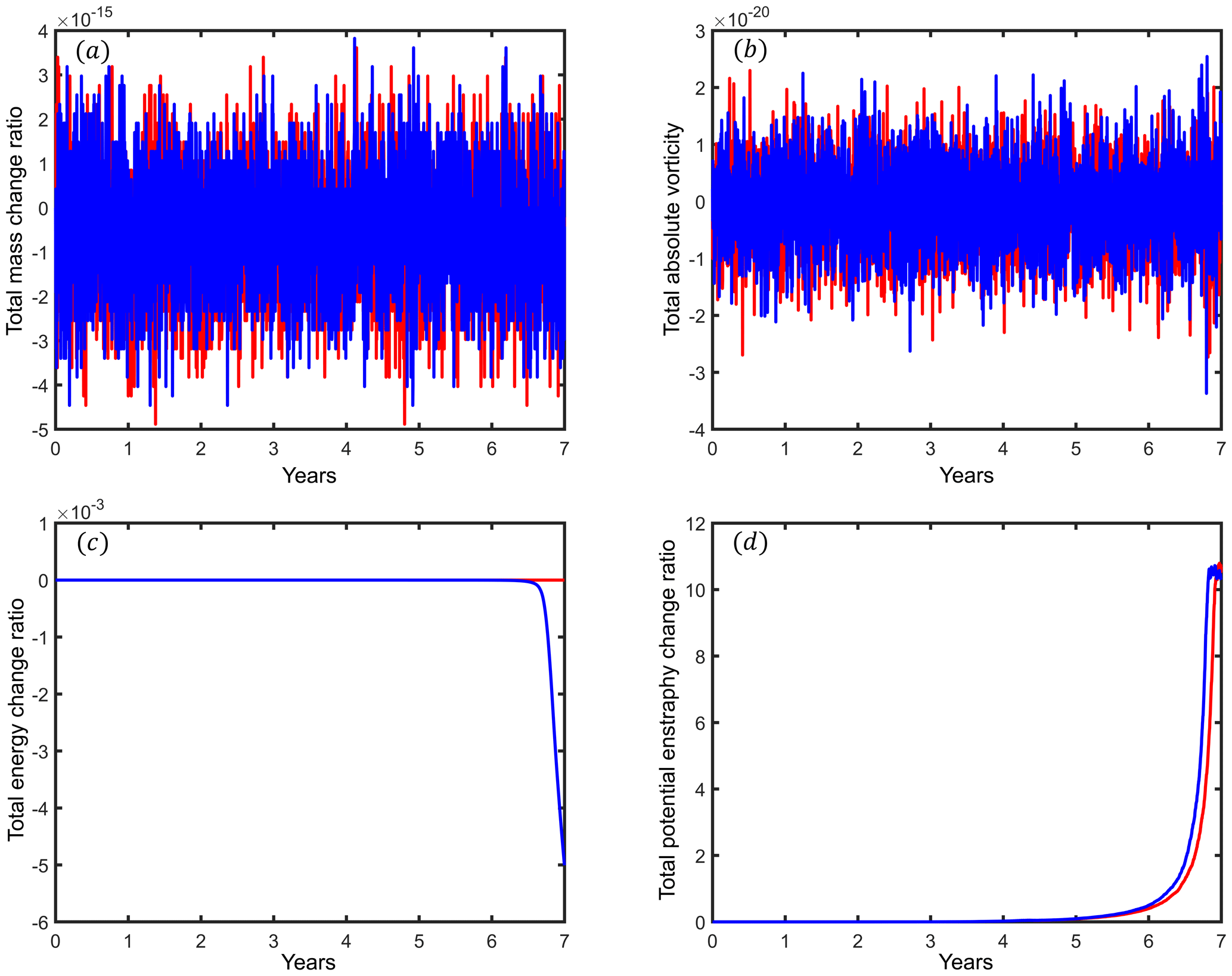
Figure 3 The variation of integral invariants as a function of time of SWTC2. (a) Total mass change ratio; (b) total absolute vorticity; (c) total energy change ratio; (d) total potential enstrophy change ratio. The results of RK4 are represented by blue lines; the results of NRK4 are represented by red lines. The model mesh is x1.2562.

5.3 Zonal flow over an isolated mountain (SWTC5)

SWTC5 is the fifth test case described by Williamson et al. (1992); the wind and height fields are similar to SWTC2, but h₀=5960 m, u₀=20 m s⁻¹ and mountain height is determined according to the following equation:

$$\begin{array}{}\text{(65)}& h_{\mathrm{s}}=h_{\mathrm{s}\mathrm{0}}\left(\mathrm{1}-{\displaystyle \frac{r}{R}}\right),\end{array}$$

where h_s0=2000 m; $R=\frac{\mathit{\pi }}{\mathrm{9}}$; $r=\sqrt{\min [R^{\mathrm{2}},(\mathit{\lambda }-{\mathit{\lambda }}_{\mathrm{c}}{)}^{\mathrm{2}}+(\mathit{\theta }-{\mathit{\theta }}_{\mathrm{c}}{)}^{\mathrm{2}}]}$; and λ_c and θ_c are the center longitude and latitude of the mountain, respectively. Here, we set ${\mathit{\lambda }}_{\mathrm{c}}=\frac{\mathrm{3}\mathit{\pi }}{\mathrm{2}}$ and ${\mathit{\theta }}_{\mathrm{c}}=\frac{\mathit{\pi }}{\mathrm{6}}$. As the analytical solution is not available, the reference solution is provided by a T511 idealized global spectral atmospheric model from GFDL, where 8×10¹² m⁴ s⁻¹ is selected as the coefficient for the ∇⁴ dissipation, and the test case is integrated for 50 d.

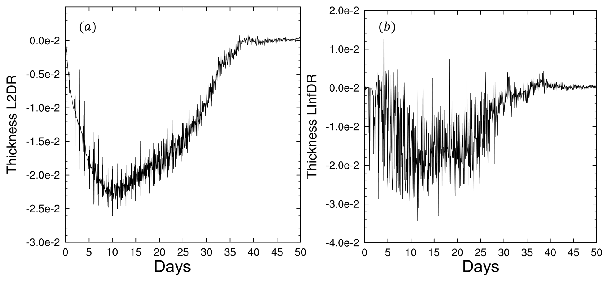
Figure 4 The different ratios of fluid thickness error norms of SWTC5. (a) L₂ error norm difference ratio; (b) L_∞ error norm difference ratio. The model mesh is x1.40962.

Figure 4 presents the different ratios of error norms. In the first 35 d, the L₂ and L_∞ error norms of NRK4 are considerably smaller than those of RK4. Compared with RK4, the L₂ error norm of NRK4 decreases by approximately 2.5 % at the minimum point of L2DR, and the L_∞ error norm also decreases by approximately 3 % at the minimum point of LInfDR. The error norms increase very quickly after 35 d; therefore, the differences between error norm ratios for NRK4 and RK4 tend to be similar, along with time.

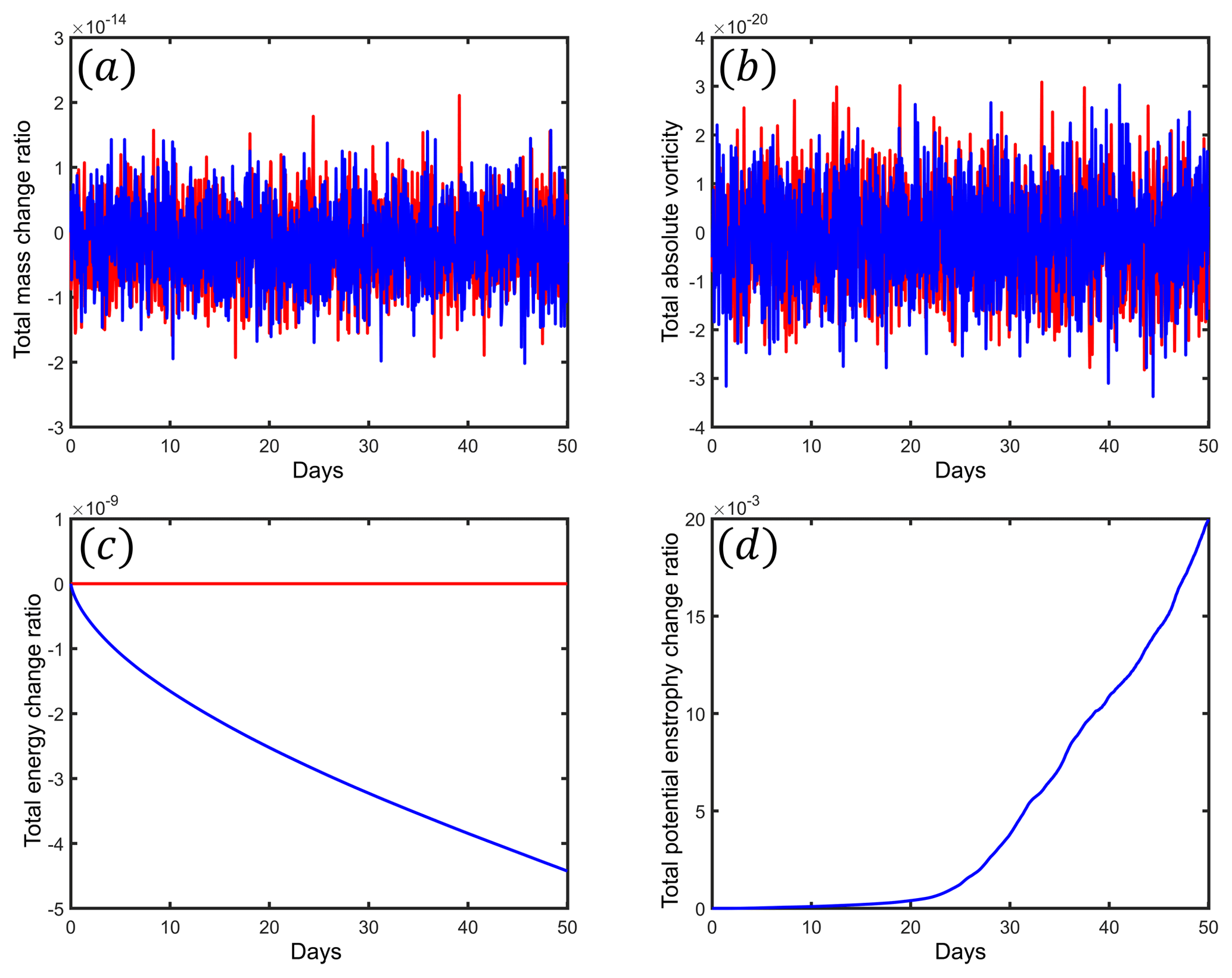
Figure 5 Integral invariants of SWTC5. (a) Total mass change ratio; (b) total absolute vorticity; (c) total energy change ratio; (d) total potential enstrophy change ratio. The results of RK4 and NRK4 are represented by blue and red lines, respectively. The model mesh is x1.40962.

Figure 5 presents the variation of the invariants as a function of time. The total mass and total absolute vorticity are completely conserved for both NRK4 and RK4. NRK4 is able to maintain strict energy conservation (at 10⁻¹⁵ magnitude) from the beginning to the end, but the total energy of RK4 is dissipative. The CSCS exhibits no influence on the total potential enstrophy.

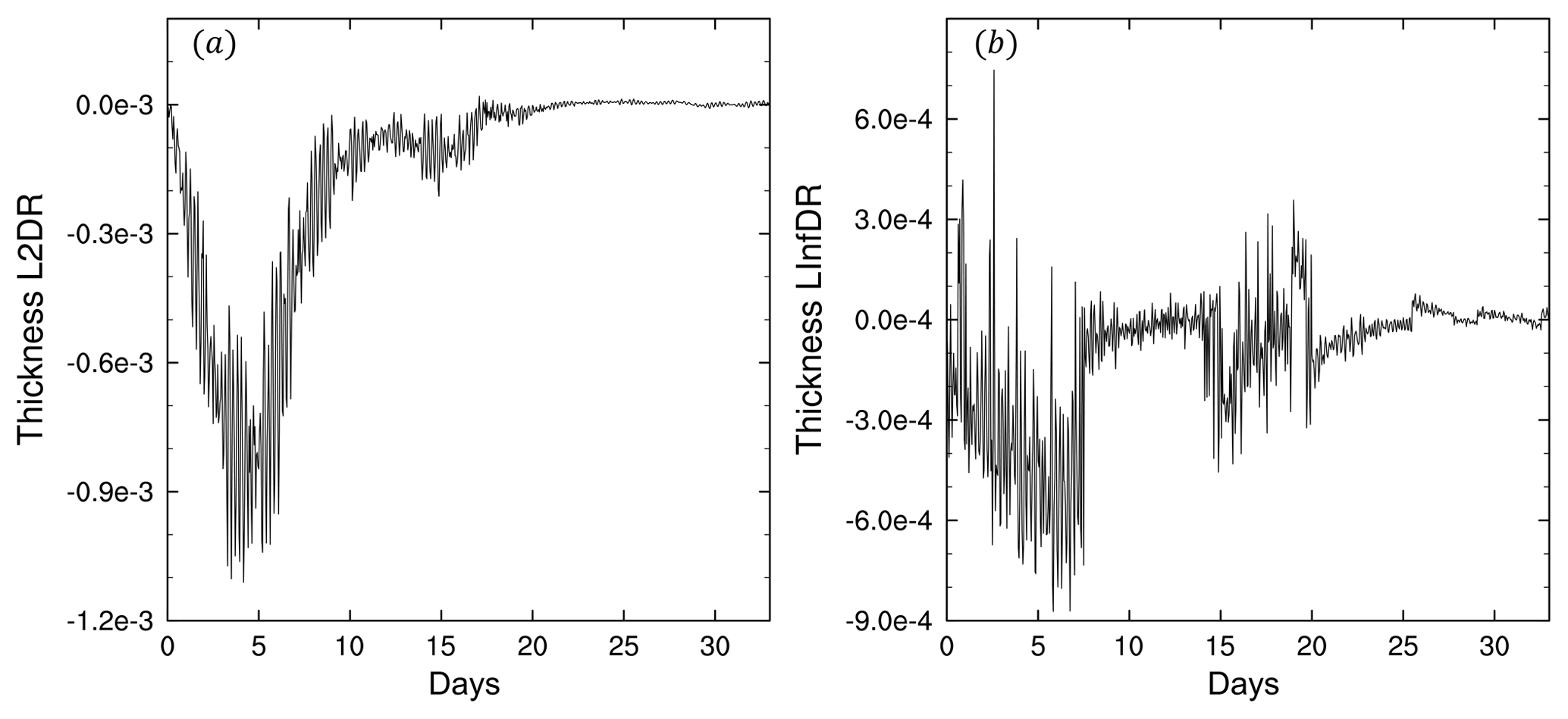
Figure 6 The different ratios of fluid thickness error norms of SWTC6. (a) L₂ error norm difference ratio; (b) L_∞ error norm difference ratio. The model mesh is x1.40962.

5.4 Rossby–Haurwitz wave (SWTC6)

The classical four-zonal wavenumber Rossby–Haurwitz wave was selected as the third test case. The initial condition follows Williamson et al. (1992). The initial state is the analytical solution of the nonlinear barotropic vorticity equation on the sphere but not the analytical solution of the shallow water equations. The reference field is provided by a T511 idealized global spectral atmospheric model from GFDL. To limit the noise of the spectral model, we use 5×10¹² m⁴ s⁻¹ as the coefficient for the ∇⁴ dissipation. As presented by Williamson et al. (1992), the phase speed of the Rossby–Haurwitz wave is calculated as follows:

$$\begin{array}{}\text{(66)}& c={\displaystyle \frac{R(R+\mathrm{3})\mathit{\omega }-\mathrm{2}\mathrm{\Omega }}{(R+\mathrm{1})(R+\mathrm{2})}},\end{array}$$

where R=4 is the zonal wavenumber of the Rossby–Haurwitz wave; $\mathit{\omega }=\mathrm{7.848}\times {\mathrm{10}}^{-\mathrm{6}}$ s⁻¹; and $\mathrm{\Omega }=\mathrm{7.292}\times {\mathrm{10}}^{-\mathrm{5}}$ s⁻¹ is the rotation rate of the earth; therefore, the four-zonal wavenumber period of the Rossby–Haurwitz wave is approximately 29.52 d. We integrate the test case over one period (33 d).

In both simulations of NRK4 and RK4, the Rossby–Haurwitz wave begins to distort on the 25th day and then collapse a few days later.

Figure 6 presents the error norm difference ratios. NRK4 has a smaller L₂ error norm than RK4 in the first 20 d. With growth of the L₂ error norm, the difference between NRK4 and RK4 trends toward zero. On the fourth day, the L₂ error norm of NRK4 is more than 0.11 % lower than that of RK4. NRK4 also has a smaller L_∞ error norm a majority of the time. On the sixth day, the L_∞ error norm of NRK4 is more than 0.08 % lower than that of RK4.

Figure 7 presents the variation of invariants as a function of time. The total mass and total absolute vorticity are strictly conserved for both NRK4 and RK4. As expected, NRK4 maintains strict energy conservation (at 10⁻¹⁵ magnitude), and RK4 cannot conserve the total energy during integration. With the Rossby–Haurwitz wave collapse, the total energy of RK4 rapidly dissipates after 25 d. There is no influence of NRK4 to potential enstrophy in this case.

The red lines and blue lines in Figs. 3c, 5c, and 7c are exactly the results of two kinds of energy conservation schemes; the blue lines present the property of conserving energy in time truncation error, and the red lines show conserving energy in the round-off error. The differences are clear to see. As mentioned above, conserving total energy in time truncation error leads to slight energy dissipation, and the dissipation accumulates during integration. Total energy may become zero after a long-term simulation, which is unreasonable for a pure dynamic core without any energy sinks or sources. On the other hand, the complete energy conservation scheme maintains strictly energy conservation in the entire integration period, even though it is not able to prevent the collapse of SWTC2, but the collapse time is delayed. Meanwhile, the simulation errors in SWTC5 and SWTC6 are reduced even in a short-term simulation.

6 Summary

In this paper, we extend the CSCS to arbitrarily structured C-grids with shallow water equations, and we estimate the performance of the CSCS by using standard shallow water test cases.

There are two prerequisites for constructing CSCS: the anti-symmetrical spatial discrete operator and the square conservative temporal integration scheme. It is difficult to directly construct an anti-symmetrical spatial discrete operator on quasi-uniform grids; therefore, we take advantage of the instantaneous energy conservation property of the spatial discrete operators, as described by Ringler et al. (2010), to obtain the anti-symmetrical operator. After the IAP transformation, the units of evolution variables are unified, and the evolution variable u_e is replaced with $U_e=\sqrt{{\mathit{\varphi }}_e}{u}_e$. According to the derivative rule (Eq. 33), the temporal trend of U_e is expressed as a combination of the temporal trends of u_e and ϕ_i, and we demonstrate that the spatial discrete operator of U_e is an anti-symmetrical operator. Then, we integrate the model with the square conservative temporal integration scheme NRK4, and the complete square conservation property is achieved.

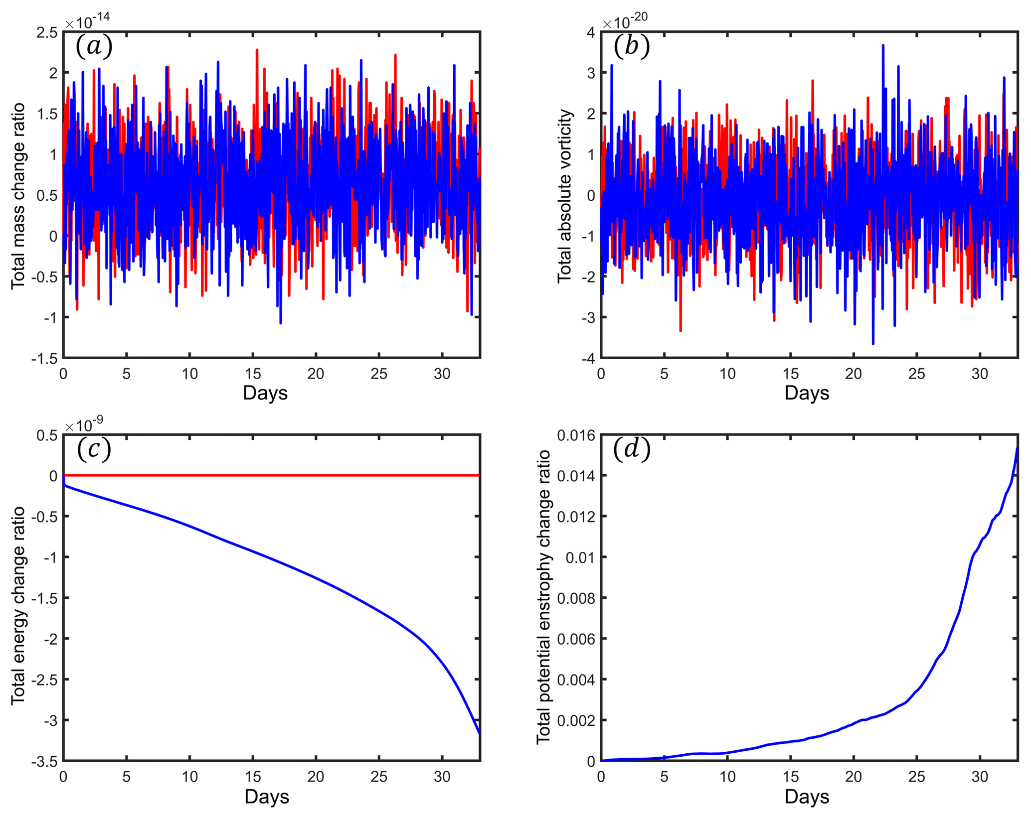
Figure 7 Integral invariants of SWTC6. (a) Total mass change ratio; (b) total absolute vorticity; (c) total energy change ratio; (d) total potential enstrophy change ratio. The results of RK4 and NRK4 are represented by blue and red lines, respectively. The model mesh is x1.40962.

An important finding is the equivalency between the energy conservative operator and anti-symmetrical operator for both the continuous system and discrete system. In most previous studies, anti-symmetrical operators were constructed on uniform grids, especially longitude–latitude grids, and the equation's advection term was in the advection flux form. We extend the square conservation theory to a more general situation. The anti-symmetrical spatial discrete operator is constructed on quasi-uniform grids, and the equation is in the vector-invariant form.

The CSCS is able to maintain three integral invariants, including total mass, total absolute vorticity and total energy, in all the test cases, and the error norms decrease to varying degrees. The square conservation scheme improves the stability in SWTC2, and the error norms of NRK4 are evidently lower than RK4 after 4 years of simulation. For RK4, the total energy dissipates very quickly after the geostrophic flow collapse, but NRK4 maintains complete energy conservation for the entire period, and the increasing rate of the total potential enstrophy is also limited by the square conservation scheme. In both SWTC5 and SWTC6, NRK4 not only maintains strict conservation for three integral invariants; it also leads to less error norms than RK4.

Appendix A

In this appendix, we attempt to demonstrate that the spatial discrete operator L is energy conservative. Our objective is to prove that the following equation is able to be satisfied by L:

$$\begin{array}{}\text{(A1)}& {\left(U,{\displaystyle \frac{\partial U}{\partial t}}\right)}_e+{\left(\mathit{\varphi },{\displaystyle \frac{\partial \mathit{\varphi }}{\partial t}}\right)}_i=\mathrm{0}.\end{array}$$

Consider the inner product on edge

$$\begin{array}{}\text{(A2)}& {\left(U,{\displaystyle \frac{\partial U}{\partial t}}\right)}_e=\sum _{e=\mathrm{1}}^{\mathrm{nEdges}}{U}_e{\displaystyle \frac{\partial U_e}{\partial t}}{A}_e.\end{array}$$

Substituting Eq. (33) into the above formula,

$$\begin{array}{}\text{(A3)}& {\left(U,{\displaystyle \frac{\partial U}{\partial t}}\right)}_e=\sum _{e=\mathrm{1}}^{\mathrm{nEdges}}{U}_e\left(C_e{\displaystyle \frac{\partial u_e}{\partial t}}+{\displaystyle \frac{u_e}{\mathrm{2}{C}_e}}{\displaystyle \frac{\partial {\mathit{\varphi }}_e}{\partial t}}\right)A_e,\end{array}$$

where $C_e=\sqrt{{\mathit{\varphi }}_e}$ is the phase speed of external gravity wave on edge e.

According to Eq. (52) in Ringler et al. (2010),

$$\begin{array}{}\text{(A4)}& {\left(U,{\displaystyle \frac{\partial U}{\partial t}}\right)}_e=\sum _{e=\mathrm{1}}^{\mathrm{nEdges}}\left({\mathit{\varphi }}_e{u}_e{\displaystyle \frac{\partial u_e}{\partial t}}+{\displaystyle \frac{u_e^{\mathrm{2}}}{\mathrm{4}}}\sum _{i\in \mathrm{CE}\left(e\right)}{\displaystyle \frac{\partial {\mathit{\varphi }}_i}{\partial t}}\right)A_e.\end{array}$$

According to Eqs. (63) and (A8) in Ringler et al. (2010),

$$\begin{array}{}\text{(A5)}& {\left(U,{\displaystyle \frac{\partial U}{\partial t}}\right)}_e=\sum _{e=\mathrm{1}}^{\mathrm{nEdges}}{\mathit{\varphi }}_e{u}_e{\displaystyle \frac{\partial u_e}{\partial t}}{A}_e+\sum _{i=\mathrm{1}}^{\mathrm{nCells}}{K}_i{\displaystyle \frac{\partial {\mathit{\varphi }}_i}{\partial t}}{A}_i.\end{array}$$

Substituting Eq. (6) into the above formula,

$$\begin{array}{}\text{(A6)}& \begin{array}{rl}{\left(U,{\displaystyle \frac{\partial U}{\partial t}}\right)}_e& =\sum _{e=\mathrm{1}}^{\mathrm{nEdges}}{\mathit{\varphi }}_e{u}_e{A}_e\left(Q_e^{\perp }+{\displaystyle \frac{\mathrm{1}}{d_e}}\sum _{i\in \mathrm{CE}\left(e\right)}{n}_{e,i}{E}_i\right)\\ & +\sum _{i=\mathrm{1}}^{\mathrm{nCells}}{K}_i{\displaystyle \frac{\partial {\mathit{\varphi }}_i}{\partial t}}{A}_i.\end{array}\end{array}$$

According to Sect. 3.7.2 in Ringler et al. (2010),

$$\begin{array}{}\text{(A7)}& \sum _{e=\mathrm{1}}^{\mathrm{nEdges}}{\mathit{\varphi }}_e{u}_e{A}_e{Q}_e^{\perp }=\mathrm{0}.\end{array}$$

Since A_e=l_ed_e,

$$\begin{array}{}\text{(A8)}& \begin{array}{rl}{\left(U,{\displaystyle \frac{\partial U}{\partial t}}\right)}_e& =\sum _{e=\mathrm{1}}^{\mathrm{nEdges}}{\mathit{\varphi }}_e{u}_e{l}_e\sum _{i\in \mathrm{CE}\left(e\right)}{n}_{e,i}{E}_i\\ & +\sum _{i=\mathrm{1}}^{\mathrm{nCells}}{K}_i{\displaystyle \frac{\partial {\mathit{\varphi }}_i}{\partial t}}{A}_i\end{array}\end{array}$$

where $E_i=K_i+{\mathit{\varphi }}_i$.

According to Eq. (A4) in Ringler et al. (2010),

$$\begin{array}{}\text{(A9)}& \begin{array}{rl}{\left(U,{\displaystyle \frac{\partial U}{\partial t}}\right)}_e& =\sum _{i=\mathrm{1}}^{\mathrm{nCells}}{E}_i\sum _{e\in \mathrm{EC}\left(i\right)}{n}_{e,i}{\mathit{\varphi }}_e{u}_e{l}_e\\ & +\sum _{i=\mathrm{1}}^{\mathrm{nCells}}{K}_i{\displaystyle \frac{\partial {\mathit{\varphi }}_i}{\partial t}}{A}_i.\end{array}\end{array}$$

According to Eq. (7),

$$\begin{array}{}\text{(A10)}& -A_i{\displaystyle \frac{\partial {\mathit{\varphi }}_i}{\partial t}}=\sum _{e\in \mathrm{EC}\left(i\right)}{n}_{e,i}{l}_e{\mathit{\varphi }}_e{u}_e.\end{array}$$

Therefore,

$$\begin{array}{}\text{(A11)}& {\left(U,{\displaystyle \frac{\partial U}{\partial t}}\right)}_e=-\sum _{i=\mathrm{1}}^{\mathrm{nCells}}{E}_i{\displaystyle \frac{\partial {\mathit{\varphi }}_i}{\partial t}}{A}_i+\sum _{i=\mathrm{1}}^{\mathrm{nCells}}{K}_i{\displaystyle \frac{\partial {\mathit{\varphi }}_i}{\partial t}}{A}_i.\end{array}$$

Consider the inner product on cell

$$\begin{array}{}\text{(A12)}& {\left(\mathit{\varphi },{\displaystyle \frac{\partial \mathit{\varphi }}{\partial t}}\right)}_i=\sum _{i=\mathrm{1}}^{\mathrm{nCells}}{\mathit{\varphi }}_i{\displaystyle \frac{\partial {\mathit{\varphi }}_i}{\partial t}}{A}_i.\end{array}$$

Thus,

$$\begin{array}{}\text{(A13)}& \begin{array}{rl}{\left(U,{\displaystyle \frac{\partial U}{\partial t}}\right)}_e& +{\left(\mathit{\varphi },{\displaystyle \frac{\partial \mathit{\varphi }}{\partial t}}\right)}_i=-\sum _{i=\mathrm{1}}^{\mathrm{nCells}}{E}_i{\displaystyle \frac{\partial {\mathit{\varphi }}_i}{\partial t}}{A}_i\\ & +\sum _{i=\mathrm{1}}^{\mathrm{nCells}}{K}_i{\displaystyle \frac{\partial {\mathit{\varphi }}_i}{\partial t}}{A}_i+\sum _{i=\mathrm{1}}^{\mathrm{nCells}}{\mathit{\varphi }}_i{\displaystyle \frac{\partial {\mathit{\varphi }}_i}{\partial t}}{A}_i=\mathrm{0}.\end{array}\end{array}$$