the Creative Commons Attribution 4.0 License.
the Creative Commons Attribution 4.0 License.
 | 25 Nov 2020
Exploring the parameter space of the COSMO-CLM v5.0 regional climate model for the Central Asia CORDEX domain
Silje Lund Sørland
Ingo Kirchner
Martijn Schaap
Christoph C. Raible
Ulrich Cubasch
The parameter uncertainty of a climate model represents the spectrum of the results obtained by perturbing its empirical and unconfined parameters used to represent subgrid-scale processes. In order to assess a model's reliability and to better understand its limitations and sensitivity to different physical processes, the spread of model parameters needs to be carefully investigated. This is particularly true for regional climate models (RCMs), whose performance is domain dependent.
In this study, the parameter space of the Consortium for Small-scale Modeling CLimate Mode (COSMO-CLM) RCM is investigated for the Central Asia Coordinated Regional Climate Downscaling Experiment (CORDEX) domain, using a perturbed physics ensemble (PPE) obtained by performing 1-year simulations with different parameter values. The main goal is to characterize the parameter uncertainty of the model and to determine the most sensitive parameters for the region. Moreover, the presented experiments are used to study the effect of several parameters on the simulation of selected variables for subregions characterized by different climate conditions, assessing by which degree it is possible to improve model performance by properly selecting parameter inputs in each case. Finally, the paper explores the model parameter sensitivity over different domains, tackling the question of transferability of an RCM model setup to different regions of study.
Results show that only a subset of model parameters present relevant changes in model performance for different parameter values. Importantly, for almost all parameter inputs, the model shows an opposite behaviour among different clusters and regions. This indicates that conducting a calibration of the model against observations to determine optimal parameter values for the Central Asia domain is particularly challenging: in this case, the use of objective calibration methods is highly necessary. Finally, the sensitivity of the model to parameter perturbation for Central Asia is different than the one observed for Europe, suggesting that an RCM should be retuned, and its parameter uncertainty properly investigated, when setting up model experiments for different domains of study.
- Article
(3728 KB) - Full-text XML
-
Supplement
(99 KB) - BibTeX
- EndNote


Climate models are representations of the climate system based on well-understood physics combined with simplified descriptions of subgrid-scale processes called parameterizations (Hourdin et al., 2017). These parameterizations usually depend on one or several empirical and unconfined parameters (Hourdin et al., 2017; Bellprat et al., 2012a; Tebaldi and Knutti, 2007) whose different values produce a wide spectrum of outcomes referred to as parameter uncertainty. Parameter uncertainty is important because it allows us to better understand model limitations and sensitivity to different physical processes. The common approach to sample model parameter uncertainty is to use ensembles of model simulations, called perturbed physics ensembles (PPEs; Murphy et al., 2007; Bellprat, 2013; Tebaldi and Knutti, 2007; Paeth, 2015).
When producing climate projections for impact studies, as much uncertainty as possible should be accounted for in order to properly drive policy-makers in their decision-making process, providing a measure of model reliability (Knutti et al., 2002, 2003; Murphy et al., 2004; Stainforth et al., 2005; Tebaldi and Knutti, 2007; Paeth et al., 2013; Bellprat, 2013; Paeth, 2015). Not properly investigating model uncertainties weakens confidence in climate projections and limits the usefulness of model outputs for adaptation strategies (Lempert et al., 2004; Foley, 2010). PPEs are of paramount importance for determining the range of model uncertainty in a probabilistic sense and assessing model reliability.
However, adequately sampling a climate model parameter space requires the performance of an extremely large number of simulations. This somehow conflicts with the need for high-resolution information for impact studies and adaptation measures at a local scale. In fact, complex high-resolution models have enormous computational demands, making it difficult to produce PPEs for future climate projections. Therefore, when willing to produce reliable (in a probabilistic sense) climate projections using high-resolution climate models such as regional climate models (RCMs), available computer resources constitute a real challenge (Paeth, 2015). A common and solid alternative practice is to use PPEs to constrain model uncertainty by selecting parameter values in a way to minimize the differences between present-day observations and model results. The determined most reliable model configuration is then assumed to be the same also in the future (Hourdin et al., 2017; Bellprat et al., 2012b). This procedure is referred to as model tuning or calibration. It is important to acknowledge that calibration techniques represent only a plausible attempt to increase model reliability for climate projections, since constraining model results based on present-day skills is not a guarantee of future skill.
In recent years, the main efforts of the climate modelling community have been channelled towards developing transparent, reproducible and objective calibration methods, using well-founded mathematical and statistical frameworks (Bellprat et al., 2012b, 2016; Hourdin et al., 2017). Among others, methods based on oracle-based optimization, ensemble Kalman filters, Markov chain Monte Carlo integrations, Latin hypercubes and Bayesian stochastic inversion algorithms have been proposed and used for climate models calibration (Price et al., 2009; Beltran et al., 2006; Jackson et al., 2004; Jones et al., 2005; Annan et al., 2005; Medvigy et al., 2010; Järvinen et al., 2010; Gregoire et al., 2011; Tett et al., 2013; Schirber et al., 2013; Ollinaho et al., 2013; Williamson et al., 2013; Annan and Hargreaves, 2007). However, most of these methods cannot be directly applied to computationally costly high-resolution climate models to exhaustively explore their parameter space, since typically hundreds of simulations have to be performed (Bellprat et al., 2012b; Hourdin et al., 2017). This led to the further development of statistical surrogate models, also referred to as model emulators or meta models (O'Hagan, 2006; Bellprat et al., 2012b; Hourdin et al., 2017). These methods have the advantage of being a computationally cheap representation of the sensitivity of the climate model to the parameter space.
One of the first objective calibration methods using such a surrogate or meta model to tune an RCM is the one of Bellprat et al. (2012a, b). Their method is mainly composed of two parts: a first one in which the model parameter uncertainty is investigated in order to determine a subsample of model most sensitive parameters, and a second one where a second-order polynomial meta model, firstly proposed by Neelin et al. (2010), is applied to extrapolate the model behaviour for all the possible values of the selected parameters and their mutual interactions. Bellprat et al. (2012b) firstly used their method for the calibration of the Consortium for Small-scale Modeling CLimate Mode (COSMO-CLM) RCM (Rockel et al., 2008) for the Coordinated Regional Climate Downscaling Experiment (CORDEX; Giorgi et al., 2009) European domain. The same method has successively been employed in the study of Bellprat et al. (2016) for investigating the transferability of the COSMO-CLM model configuration to other regions such as the North America CORDEX domain and for the tuning of the same model for high-resolution numerical weather predictions over western Europe (Voudouri et al., 2017, 2018).
In this work, the results of a PPE conducted for the year 2000 with COSMO-CLM v5.0 for the Central Asia CORDEX domain are presented, with the main objective of investigating the model parameter uncertainty for the area and setting the basis for the application of the objective calibration method of Bellprat et al. (2012b). Central Asia is particularly important from both a climate impact and modelling perspective (Russo et al., 2019). Nonetheless, only few studies have been conducted for this area using RCMs (Ozturk et al., 2012, 2017; Russo et al., 2019) and more efforts are indeed required for better characterizing models uncertainties and limitations. Here, the results of the proposed PPE are used in order to (1) determine the most sensitive COSMO-CLM parameters for the area, on which to apply the calibration method of Bellprat et al. (2012b) and (2) to investigate the relevance of different physical processes for different regions, assessing at the same time how much model deficiencies can be ameliorated by properly setting parameter values in each case. Additionally, the results are used to (3) address the highly debated question of transferability of RCM configuration to a different domain of interest (Takle et al., 2007; Jacob et al., 2007, 2012; Rockel and Geyer, 2008; Bellprat et al., 2016).
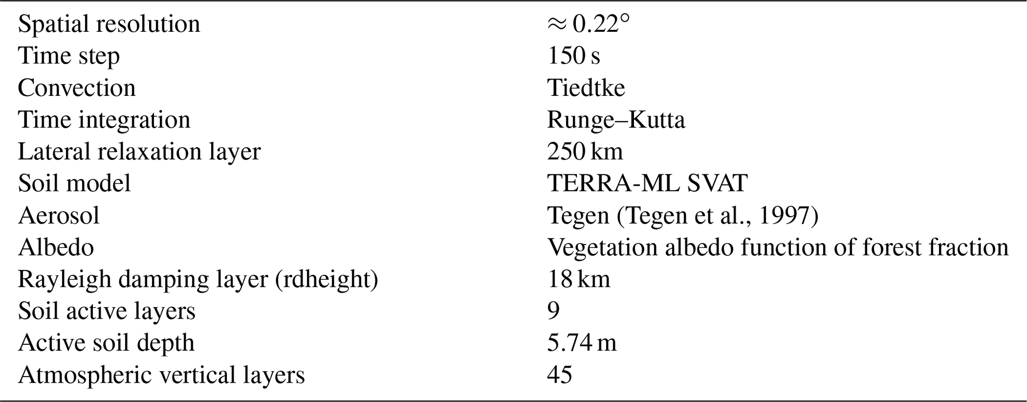
(Tegen et al., 1997)Table 1General description of model setup of the reference simulation.
The study is structured as follows. In Sect. 2, the model and sensitivity simulations as well as the considered metrics are introduced. Then, the model parameter sensitivity for the entire domain is discussed in Sect. 3.1, while subregional model deficiencies are characterized in Sect. 3.2. A discussion on the role of different uncertainty sources on the considered metrics is presented in Sect. 3.3. By comparing the Central Asia setting with results obtained for the European CORDEX domain, the transferability of the model configuration between different domains is addressed in Sect. 3.4. Finally, the results are summarized and conclusive remarks are presented in Sect. 4.
2.1 Model and experiments
For the simulations over Central Asia presented in this study, the COSMO-CLM version 5.0_clm9 regional climate model is used. COSMO-CLM is the climate version (Rockel et al., 2008) of the non-hydrostatic model COSMO, developed for numerical weather predictions (Baldauf et al., 2011; Doms and Baldauf, 2013; Doms et al., 2013). It is based on the primitive thermohydrodynamical equations describing compressible flow in a moist atmosphere and takes into account a variety of physical processes through different parameterization schemes.
The applications of COSMO-CLM range from palaeoclimate (Russo and Cubasch, 2016; Fallah et al., 2016; Prömmel et al., 2013) to future projections (Dosio et al., 2015; Dosio and Panitz, 2016; Bucchignani et al., 2016, 2014; Fischer et al., 2013; Dobler and Ahrens, 2011; Wang et al., 2013; Keuler et al., 2016; Sørland et al., 2018) and span a large variety of spatial resolutions, from mesoscales to convection-permitting scales (Fosser et al., 2015; Knote et al., 2010; Brisson et al., 2015; Tölle et al., 2014; Ban et al., 2015).
The model is used in this study at a spatial resolution of 0.22∘, following the framework of the new CORDEX Coordinated Output for Regional Evaluations (CORDEX-CORE) initiative (Gutowski Jr. et al., 2016; see https://www.cordex.org/experiment-guidelines/cordex-core/, last access: 1 May 2020).
The simulations used for characterizing the model parameters uncertainty are 1 year long and are run from an equilibrium state obtained from a 10-year simulation over the period of 1991–2000. This simulation represents the reference simulation for this study. Its configuration is derived from Russo et al. (2019) and uses a representation of vegetation albedo taking into account forest fraction and soil heat conductivity accounting for soil ice–moisture ratio. Table 1 provides a summary of the reference simulation setup. A more detailed description of the model domain (showed in Fig. 1) and reference configuration is presented in Russo et al. (2019). Bellprat et al. (2012a) demonstrated that, for some predefined metrics, COSMO-CLM results converge already after 1 year. Therefore, for the purpose of determining the most sensitive model parameters, although perturbed physics experiments should ideally cover 3–5 years, 1-year simulations could be enough, especially when computational resources are limited. Here, the year 2000 has been selected, since it can be considered normal in terms of monthly values of the investigated variables.
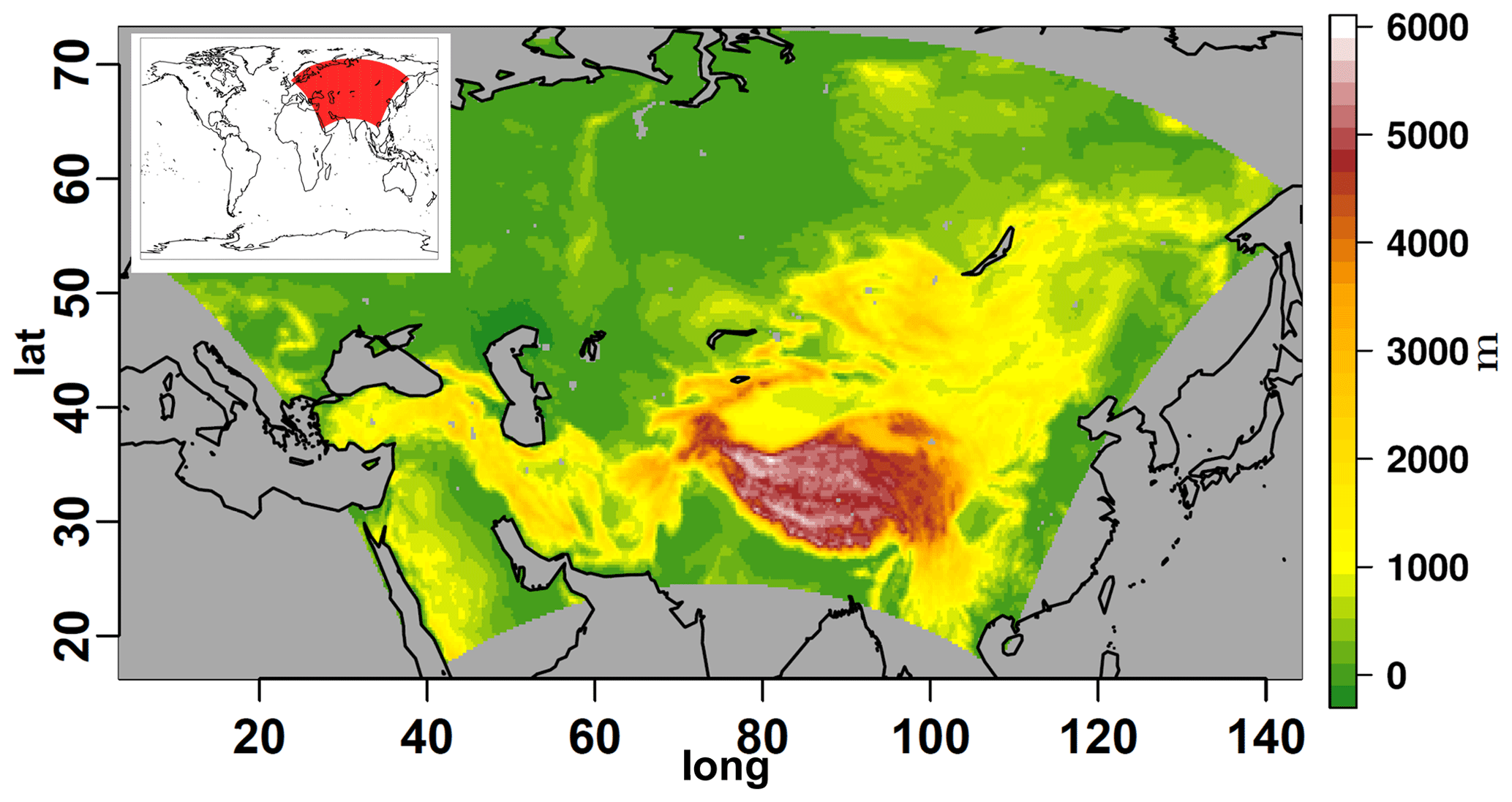
Figure 1Location and orography map of the Central Asia domain, at a spatial resolution of 0.22∘. Orographic data are derived from the Global Land One kilometre Base Elevation (GLOBE; Hastings et al., 1999) data set.
Table 2List of model parameters and corresponding ranges of investigated input values. The parameter values of the default model configuration are reported in bold. The finally selected COSMO-CLM most-sensitive parameters for the region are underlined.
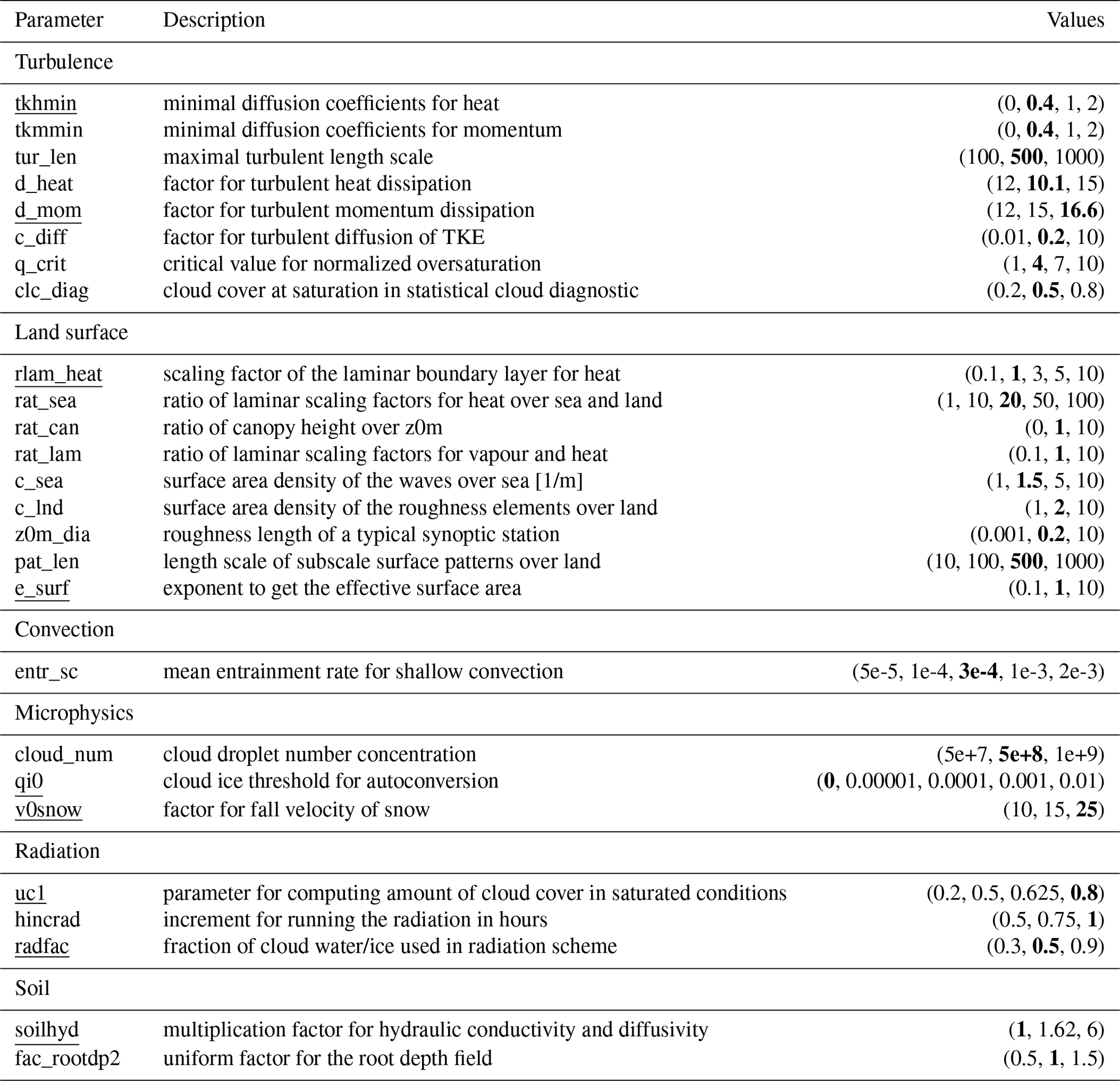
The tested parameter inputs are selected from a plausible range derived from Bellprat et al. (2012a), with a minimum, a maximum and different intermediate values, depending on the parameter. A list with all the tested values is presented in Table 2, for a total number of 92 simulations.
For the analysis, an estimate of the internal variability of the model is needed. Thus, an ensemble of five simulations covering the period of 1991–2005 but with different initial conditions (starting date shifted by ±1 and ±3 months), performed by Russo et al. (2019), is additionally considered.
To investigate the model transferability to a different domain, the same 1-year perturbed simulations are performed for four parameters for the European CORDEX domain, yielding an additional 15 simulations. An ensemble of five 15-year simulations with different initial conditions is also performed for Europe in order to estimate the model internal variability for the region.
All the presented simulations are driven by National Centers for Environmental Prediction (NCEP) version 2 (NCEP2) reanalysis data (Kanamitsu et al., 2002). NCEP2 data have a temporal resolution of 6 h and a spectral resolution of T62 (∼ 1.9∘). Within CORDEX, ERA-Interim reanalysis data are usually used to drive RCMs evaluation and calibration experiments. NCEP2 data are employed in this study, with the specific purpose of reproducing the spatial resolution jump present when using the global circulation models (GCMs) normally employed in CORDEX simulations (∼ 200 km, Russo et al., 2019).
2.2 Observations
The presented analyses focus on three variables: near-surface temperature (T2M), daily precipitation (PRE) and total cloud cover (CLCT). While T2M and PRE are highly relevant for climate impact studies, the third one is used to evaluate models' ability in simulating radiative processes (Bellprat et al., 2012a, b, 2016).
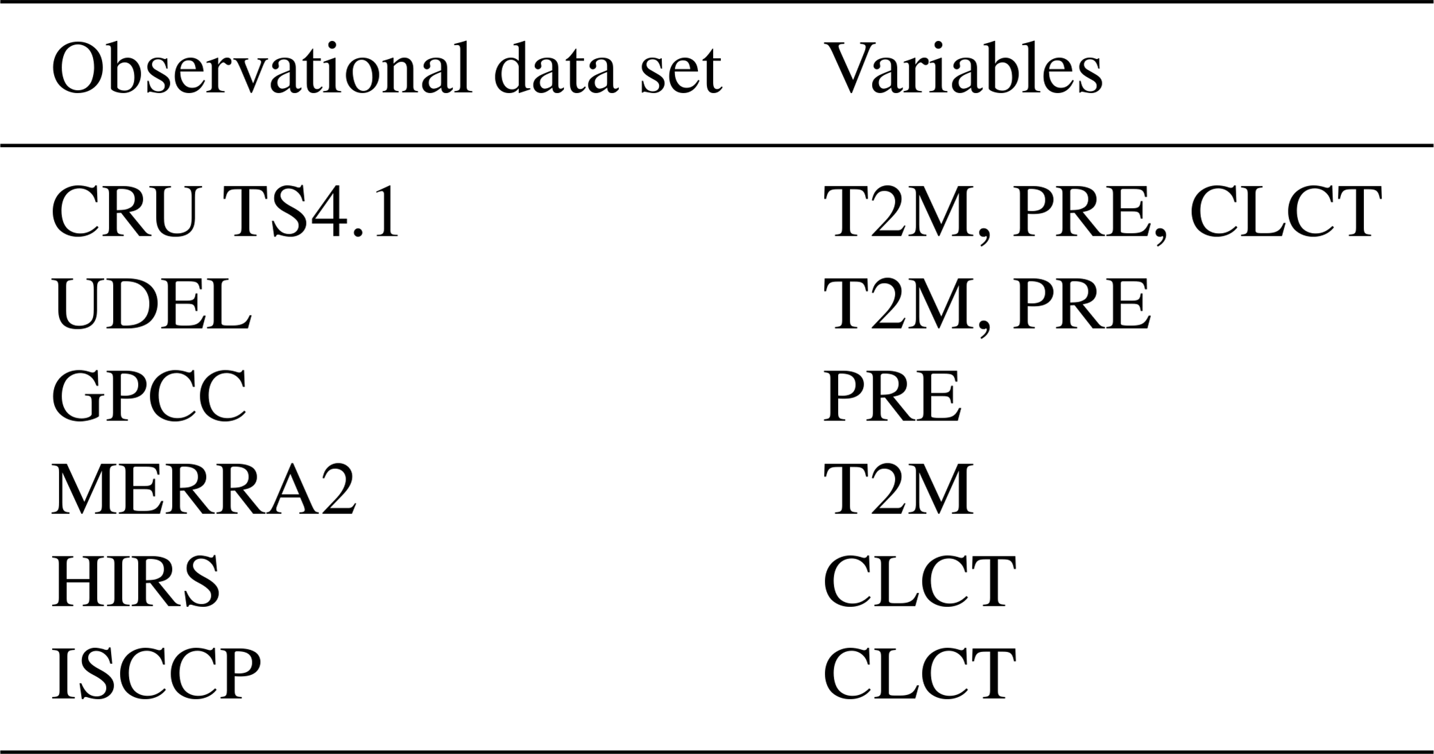
Table 3List of observational and reanalysis data sets employed for the evaluation of model results.
The range of three different observational data sets is considered for each of the variables to represent observational uncertainties (Collins et al., 2013; Gómez-Navarro et al., 2012; Bellprat et al., 2012a, b; Flaounas et al., 2012; Lange et al., 2015; Zhou et al., 2016; Solman et al., 2013; Russo et al., 2019):
-
For temperature, information is retrieved from the Climate Research Unit time series (CRU TS4.1) observational data set (Harris and Jones, 2017), from the University of Delaware (UDEL) gridded data set (Willmott, 2000), provided by the NOAA/OAR/ESRL PSD, Boulder, Colorado, USA, from their web site at https://www.esrl.noaa.gov/psd/ (last access: 1 February 2020) and from the Modern-Era Retrospective analysis for Research and Applications version 2 (MERRA2) (Gelaro et al., 2017).
-
Information on precipitation is retrieved from the CRU and the UDEL data sets, as well as from the Global Precipitation Climatology Centre (GPCC) data set (Becker et al., 2011).
-
For total cloud cover, again the CRU data set is used. Additionally, the cloud data sets extracted from the National Oceanic and Atmospheric Administration (NOAA) High Resolution Infrared Radiation Sounder (HIRS) (Wylie et al., 2005) and the International Satellite Cloud Climatology Project (ISCCP) gridded data set (Zhang et al., 2004) are used, similarly to Bellprat et al. (2012a, b).
All data sets present a spatial resolution of 0.5∘, except the HIRS and the ISCCP, having both a spatial resolution of 1∘. In the latter case, the data are interpolated on the CRU grid by means of a conservative remapping method prior to the analyses. The considered observational data sets and the corresponding variables for which they are used are reported in Table 3.
2.3 Analysis methods and evaluation metrics
The analyses are conducted on the regional means of monthly values of the considered variables for different regions characterized by differing climate conditions. By averaging, the model residuals with respect to observations become quasi-Gaussian, allowing the use of normal estimators of model disagreement (Von Storch and Zwiers, 2001; Bellprat et al., 2012a). Before spatially averaging, model results are first upscaled to the same 0.5∘ grid of the CRU observational data set by means of a bilinear remapping method in the case of temperature and through conservative remapping for the other two variables.
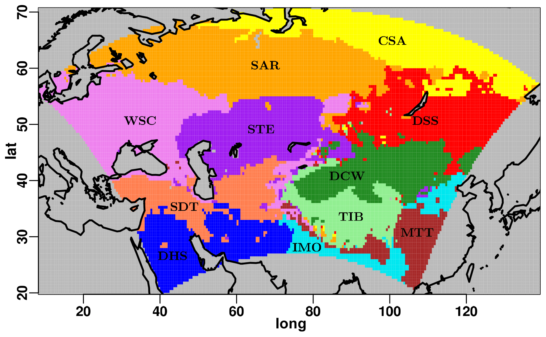
Figure 2Map of the 11 subregions obtained through k-means clustering of q-normalized monthly climatologies of the three considered variables over the period of 1996–2005.
A k-means clustering technique (Steinhaus, 1956; Ball and Hall Dj, 1965; MacQueen, 1967; Lloyd, 1982; Jain, 2010) applied onto quantile-normalized (q-normalized) monthly climatologies of the investigated variables is used to decompose the domain into a set of subregions with different climate conditions. K-means clustering allows the separation of similar data into groups, using the concept of Euclidean distance from the centroids of a predetermined group of clusters. Following several tests and the results of other studies (Mannig et al., 2013; Russo et al., 2019), a total number of 11 clusters have been selected for the Central Asia domain. As input for the clustering procedure, q-normalized values of monthly climatologies of T2M and CLCT derived from the CRU data set and PRE values derived from the GPCC are used. The results of the k-means clustering are shown in Fig. 2.
The metrics used for investigating the COSMO-CLM parameters' uncertainty is the performance index (PI) presented in Bellprat et al. (2012a) and derived from the Climate Performance Index (CPI) of Murphy et al. (2004). PI represents a normalized multivariate root-mean-square error (RMSE), weighted over different sources of uncertainties and averaged over the model variables, the considered regions and the months of a selected year:
where V=3 represents the number of variables considered, R=11 is the number of the domain subregions, and T=12 is the number of months of the given year. The terms m and o represent the model and the observational monthly means calculated for each variable, month and region. σo is the monthly SD of the interannual variations calculated from the observations over the period of 1996–2005; σiv is the monthly SD of the internal variability of the regional model for the same period; σϵ is the monthly SD of the observational error derived from different reference data sets, for the selected year.
PI represents an objective measure of model reliability, where higher (lower) values indicate bad (good) performance. In order to make inferences about the sensitivity of model parameters, Bellprat et al. (2012a, b) used the PI to define a positive performance score (PS) that can be interpreted as an approximation of the likelihood that the residuals come from a distribution with zero mean and variance given by σo, σiv and σϵ:
Basically, PI allows us to quantify model parameter uncertainty, while PS is used as an estimate of the model sensitivity to each single tested parameter.
In this study, first PI and PS are calculated for the three considered variables together. Then, given the assumption that changes in PS are expected to be smooth (Bellprat et al., 2012a; Neelin et al., 2010), a quadratic regression is fitted to the obtained values of PS for each parameter, representing an estimate of model sensitivity for that specific parameter. Successively, the same analyses are repeated for each variable separately, taking into account the fact that the obtained PS values might be due to a compensation effect of the results for single variables. This will contribute to discriminate the model most sensitive parameters for the region.
In a successive step, model parameter uncertainties for different areas of the domain are investigated. For this purpose, PI is calculated separately for each variable and subregion. Then, the variable and region dependent PI is expressed with respect to the one of the reference simulation using a skill score (SS) defined as
Positive (negative) SS values indicate an improvement (worsening) of the considered experiment over the reference simulation, in terms of the proposed metrics PI.
The range of different errors and their effects on the considered metrics will be additionally investigated to support the presented analyses.
Finally, for the comparison of the model results obtained for Central Asia with the ones for Europe, the same PS metrics, calculated for a subset of selected parameters over the entire domain, will be considered.
3.1 Sensitivity of the model to parameter perturbation for the entire domain
First, the PS for each parameter, when considering T2M, PRE and CLCT together, is investigated (Fig. 3). It is clearly seen that model performance is sensitive to only a restricted set of parameters, which is in agreement with the findings of Bellprat et al. (2012a). The parameters that have the largest impact on PS are e_surf, representing the exponent to get the effective surface area used in the land-surface scheme, and qi0, which is the parameter for the cloud ice threshold for autoconversion used in the microphysics parametrization scheme. Other parameters, which have some considerable impact on PS, are d_mom, the factor for turbulent momentum dissipation, v0snow, controlling the fall velocity of snow, radfac, which represents the fraction of cloud water/ice used in the radiation scheme, tkhmin, the minimum value for the turbulence heat diffusion coefficient, and rlam_heat, the scaling factor of the laminar boundary layer for heat. Thus, for each parametrization scheme, excluding convection, there is at least one or two parameters that show the potential to sensibly improve model performance when an optimal value is set. For some of the parameters such as c_diff, the factor for turbulent diffusion in the turbulent kinetic energy (TKE) scheme, and z0m_ dia, representing the roughness length of a typical synoptic station used for the interpolation of values of the 10 m wind, strong changes in PS are evident in Fig. 3. However, in these cases, the model performs similarly for all tested inputs, suggesting that the evinced sensitivity is an artificial result of the quadratic interpolation. Changes in PS are also evident for soilhyd, a multiplying factor for soil hydraulic conductivity and diffusivity, fac_rootdp2, an uniform factor for the root depth field, tur_len, defining the maximal turbulent length scale, uc1, used for computing the amount of cloud cover in saturated conditions, q_crit, representing the critical value for normalized oversaturation, and rat_lam, which is the ratio of laminar scaling factors for vapour and heat. For all other parameters, variations of PS are considerably small or zero.
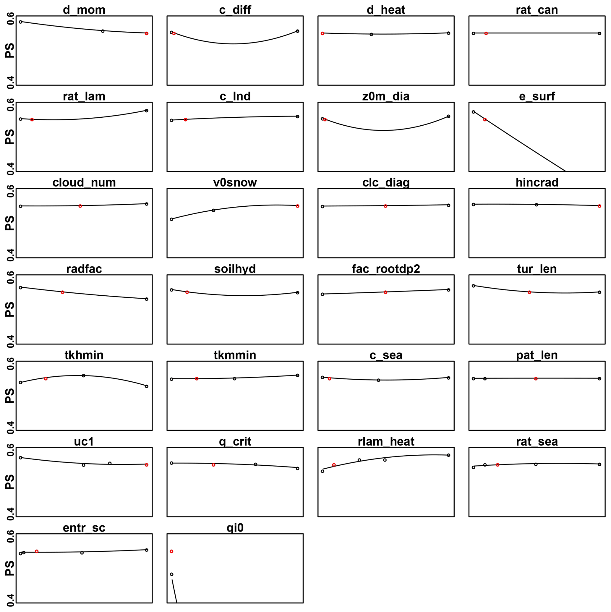
Figure 3PS calculated for near-surface temperature (T2M), daily precipitation (PRE) and total cloud cover (CLCT) together, for all the different tested parameter values, over the entire Central Asia domain. The red marks represent the PS values obtained for the default configuration.
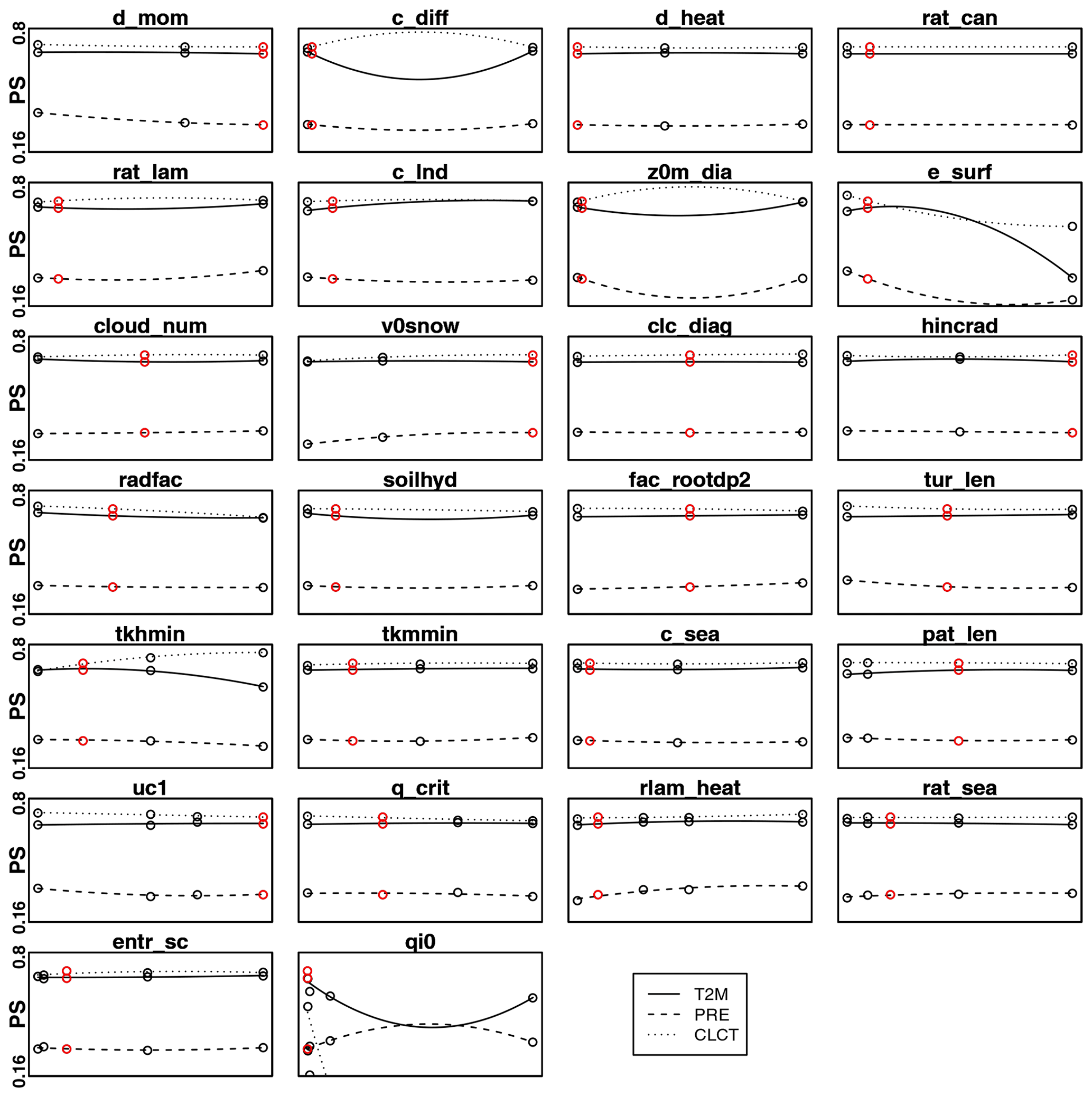
Figure 4PS calculated separately for near-surface temperature (T2M, solid line), daily precipitation (PRE, dashed line) and total cloud cover (CLCT, dotted line), for all the different tested parameter values, over the entire domain.
When investigating how PS depends on each variable (Fig. 4), similar results are obtained for all the parameters. The largest variations in PS are evident, for each of the variables, for e_surf and qi0. Remarkable changes in PS for T2M are also identified for tkhmin. In this case, also c_diff shows significant changes but, as already stated above, the PS seems to be at its maximum for the parameter values' lower and higher limits, suggesting that any parameter input in this range will not produce an improvement in temperatures. For PRE, more pronounced variations of PS are also found for d_mom, v0snow and rlam_heat. Finally, for CLCT, considerable changes in PS are also evident for tkhmin, showing an opposite behaviour with respect to the one of temperatures. Other parameters are characterized by particularly small variations in the PS calculated for single variables, but these changes are coherent among all the different variables and translate into slightly larger changes in the PS calculated over the three variables together. This is the case of radfac, soilhyd, tur_len, rat_lam, uc1 (Fig. 3). In all other cases, variations of the PS calculated for different variables compensate each other, leading to really small or zero changes in the total PS. In general, it is important to notice that the values of PS are lower for PRE than for the other two variables. Further considerations for these differences and for their possible drivers will be discussed in the next sections.
Based on these results, the nine most sensitive model parameters for the region, highlighted in blue in Table 2, are identified. A maximum of two parameters is selected for each of the model physical schemes (turbulence, surface, soil, radiation and grid-scale cloud precipitation), excluding convection, for which the only tested parameter (entr_sc), representing the mean entrainment rate for shallow convection, leads to really similar results for all the considered inputs. Despite acknowledging the importance for the region of additional parameters such as tur_len and rat_lam, a constraint to the number of selected parameters is necessary, considering the high costs in terms of computational resources needed for a calibration procedure.
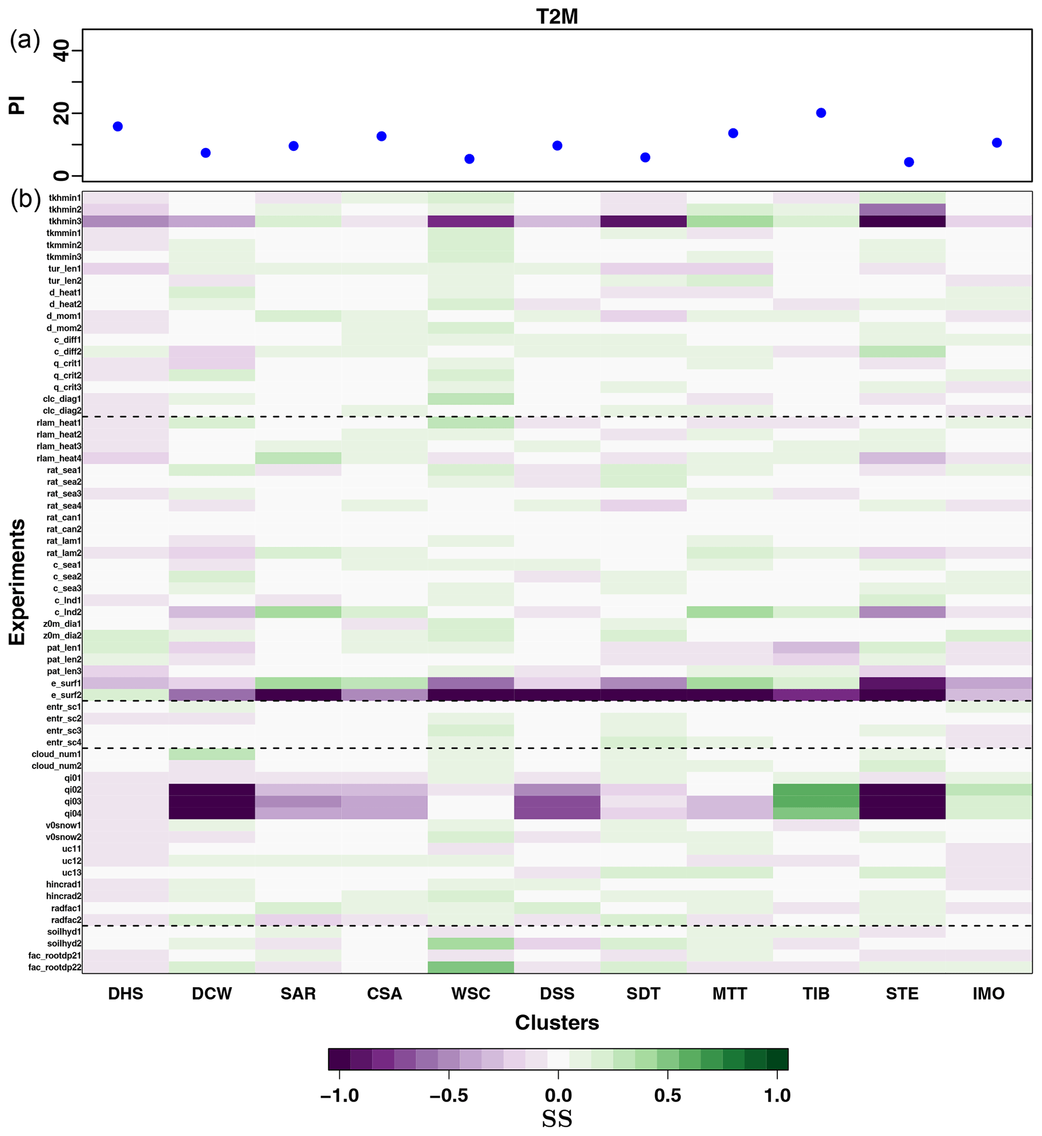
Figure 5(a) PI calculated for near-surface temperature (T2M) for the reference experiment with default parameter values, over each of the 11 Central Asia subregions. (b) Changes in the SS of each performed experiment, calculated with respect to the default simulation, for near-surface temperature (T2M): green (violet) values indicate a better (worse) agreement with observations with respect to the default simulation. The experiments for each parameter are enumerated in an increasing order, according to its tested values, from the lowest to the highest. The different simulations are additionally grouped depending on the main physical scheme the tested parameter is characteristic of, in the same way as they are in Table 2.
Thus, to properly set an optimal model configuration for the Central Asia domain, the selected nine parameters are recommended to conduct the objective calibration procedure of Bellprat et al. (2012b).
3.2 Model behaviour for different subregions
Once the most sensitive model parameters for the area are identified, a more detailed analysis of simulation results for each variable and subregion is performed. The aim is to investigate the model parameter uncertainties for regions characterized by different climate conditions, determining the most relevant processes in the model formulation in each case and assessing to which degree it is possible to improve model performance for the considered variables by properly setting parameter values.
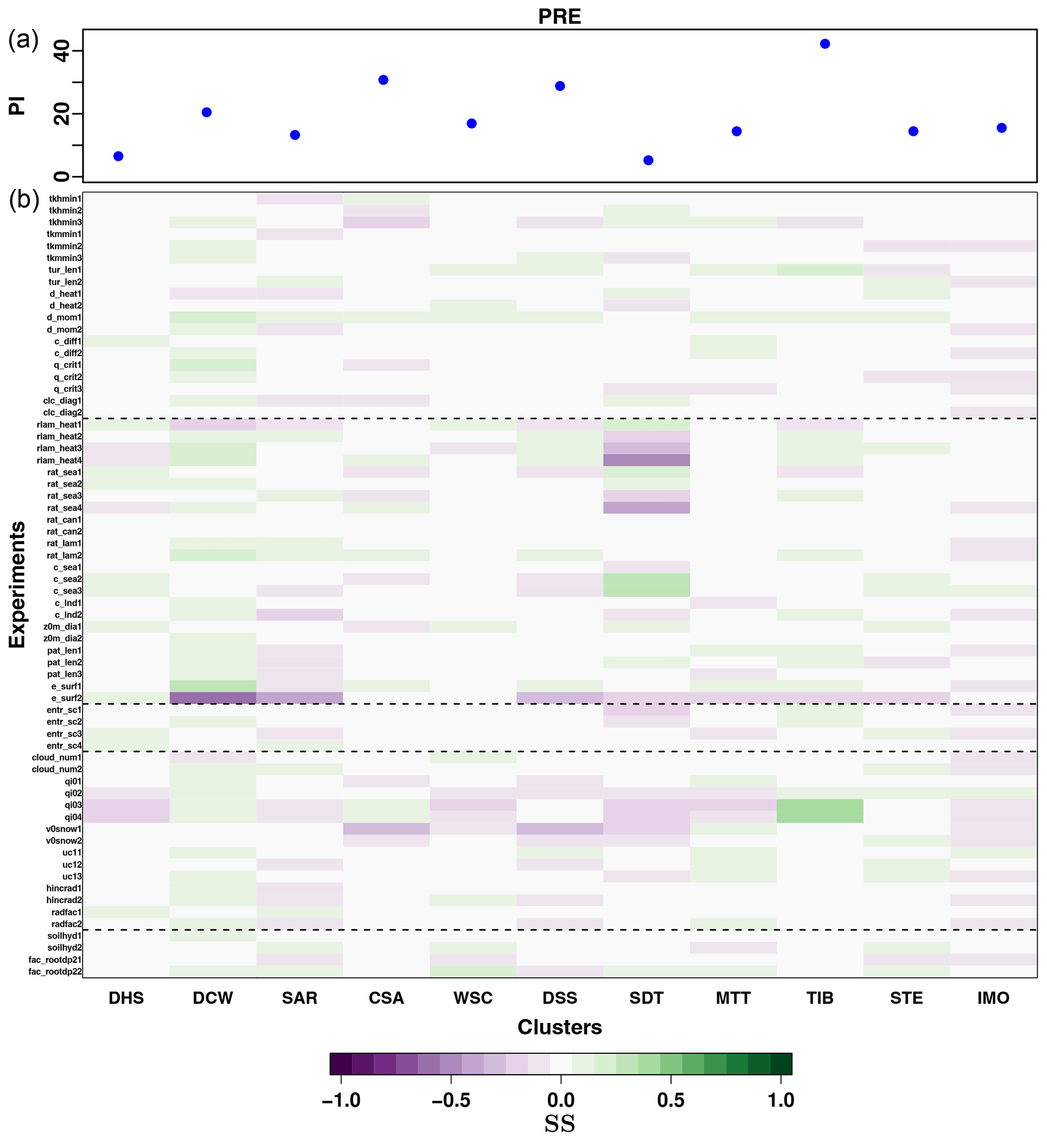
Figure 6(a) PI calculated for precipitation (PRE) for the reference experiment with default parameter values, over each of the 11 Central Asia subregions. (b) Changes in the SS of each performed experiment, calculated with respect to the default simulation, for PRE: green (violet) values indicate a better (worse) agreement with observations with respect to the default simulation. The experiments for each parameter are enumerated in an increasing order, according to its tested values, from the lowest to the highest. The different simulations are additionally grouped depending on the main physical scheme the tested parameter is characteristic of, in the same way as they are in Table 2.
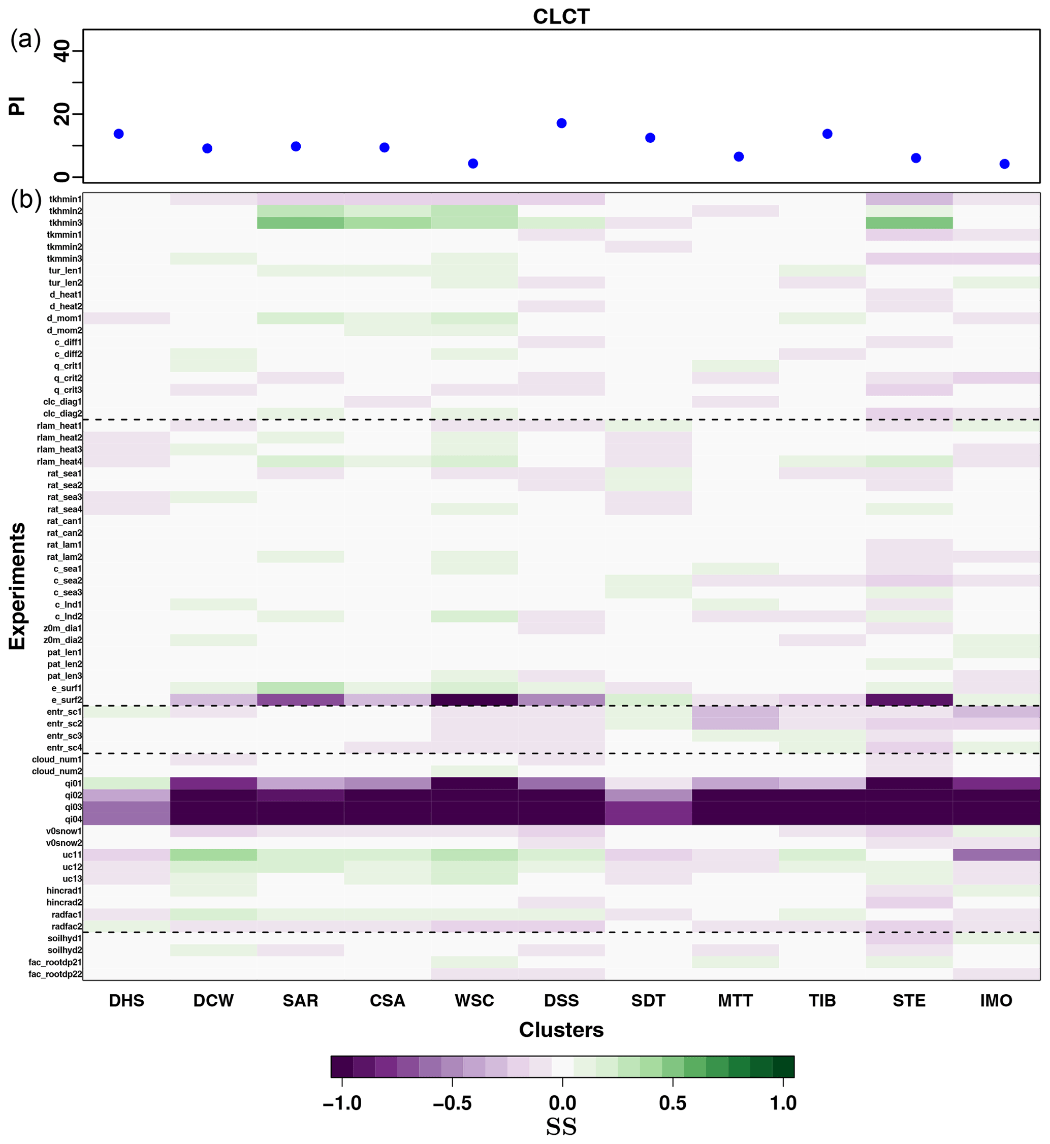
Figure 7(a) PI calculated for total cloud cover (CLCT) for the reference experiment with default parameter values, over each of the 11 Central Asia subregions. (b) Changes in the SS of each performed experiment, calculated with respect to the default simulation, for CLCT: green (violet) values indicate a better (worse) agreement with observations with respect to the default simulation. The experiments for each parameter are enumerated in an increasing order, according to its tested values, from the lowest to the highest. The different simulations are additionally grouped depending on the main physical scheme the tested parameter is characteristic of, in the same way as they are in Table 2.
Figures 5a, 6a and 7a show the PI calculated for the reference simulation (simulation with default values, highlighted in red in Table 2) for each of the subregions for T2M, PRE and CLCT, respectively, and the changes in the SS, for each cluster and performed experiment (Figs. 5b, 6b and 7b). The figures illustrate the magnitude of model deficiencies for the reference simulation, allowing us to evaluate at the same time parameter sensitivity for each subregion and variable. The high PI values are evident for PRE, confirming that the model performance is particularly poor with respect to this variable.
Figure 5a shows that the largest mismatches between the reference simulation and observations, in terms of T2M, are found over the Tibetan Plateau (TIB; Fig. 2). This particularly strong cold bias in temperature over the Tibetan Plateau, found for all seasons, is a common feature of several RCMs, as discussed in Russo et al. (2019). Some studies highlighted the importance of a better representation of surface features and processes for the Tibetan Plateau, characterized by particularly complex topography (Meng et al., 2018; Zhuo et al., 2016). Here, the results indicate that, for COSMO-CLM, parameters characteristic of surface parameterizations play only a secondary role for the simulation of T2M over the region, with pronounced changes in model performance evident only for few parameters such as e_surf and pat_len, with the latter expressing the length scale of subscale surface patterns over land. The largest improvements in the COSMO-CLM simulation of T2M over the Tibetan region are obtained for the parameter qi0, characteristic of the cloud grid-scale condensation (microphysics) physical scheme. Additionally, large variations in SS are also obtained for the same region for the parameter tkhmin. Another region where microphysics parameterizations and the characterization of cloud grid-scale condensation lead to an improvement in the simulated T2M is the northern Indian monsoon (IMO; Fig. 2) area. Particularly high values of PI for T2M are also evident in Fig. 5a, for the Arabian Peninsula and the southern Iran region (DHS; Fig. 2): no clear improvements in model results relative to this variable can be obtained for this region by perturbing parameter values (Fig. 5b). This suggests that possible model deficiencies in this case are likely related to the model formulation itself. This seems to also be the case for the northern part of the domain, corresponding to Western Siberia (SAR, CSA and DSS; Fig. 2). Russo et al. (2019) showed that COSMO-CLM presents particularly poor performance in the simulation of temperatures over Western Siberia, specifically for winter, with warm biases deriving from the comparison against observations exceeding 15 ∘C over some points. The presented analyses show that changes in PI for T2M are quite consistent among the considered Western Siberian subdomains. In this case, improvements in model performance for the simulation of T2M in terms of PI are limited to a few parameters. When the Western Siberian subregions are considered together, the main improvements are obtained for rlam_heat, radfac, hincrad, c_lnd and e_surf, indicating the importance of surface and soil features and processes related to heat fluxes for the simulation of temperature over the area. Nevertheless, these changes do not seem to be large enough to significantly reduce the T2M model bias over Western Siberia, pointing at a possible structural problem in the model formulation. For all other regions, there seems to be some potential to improve model performance in simulating T2M, by properly choosing parameter values. The largest positive values of SS are obtained for the northern Black Sea (WSC) region and the transition zone between the northern Indian monsoon and the Tibetan region (MTT). For T2M, no parameter value seems to lead to an univocal positive model response over all the different clusters together. For most of the regions, properly calibrating the parameters qi0, tkhmin and e_surf is particularly important in order to avoid significantly poor model performance in the simulation of T2M.
For PRE (Fig. 6), the amplitude of changes in the calculated SS is smaller than for T2M and CLCT. The region for which an important improvement in model performance is possible, for almost all considered parameters, is the region covering the desert areas of Mongolia and northwestern China (DCW; Fig. 2). Large improvements in the simulation of PRE are also possible for the region covering the northern part of Iran and Turkey (SDT; Fig. 2) where moisture is mainly advected by westerlies from the Mediterranean Sea (Fernández et al., 2003; Fallah et al., 2015). In this case, the model seems particularly sensitive to changes in the parameter c_sea, describing the surface area density of the waves over sea, used for the calculation of roughness length. The roughness of the sea surface steers the exchange of momentum, moisture and heat between ocean and atmosphere (Carlsson et al., 2010; Vickers and Mahrt, 2010). Thévenot et al. (2016) demonstrated that an increase in sea surface roughness may generate higher momentum fluxes, impacting low-level atmospheric dynamics, particularly affecting wind speeds, and that a proper representation of the sea surface roughness may lead to a better localization of heavy precipitation. For the northern part of Iran and Turkey, the other parameter for which the model is most sensitive to the simulation of PRE is rat_sea, the ratio of laminar scaling factors for heat over sea and land, confirming again the importance of the representation of ocean–atmosphere interactions for the simulation of precipitation over the region. Finally, significant improvements in simulated PRE are obtained for the TIB (Fig. 2), for the parameter qi0, affecting cloud microphysics, as previously described. For all other regions, changes in model performance for the simulation of PRE are not particularly remarkable, making any assumption on parameter selection almost equivalent. Only the parameter d_mom seems to be able to produce small, but positive, improvements with respect to the reference simulation, for all the clusters.
For CLCT, changes in the SS are significant only for a specific subset of parameters (Fig. 7). In particular, for qi0, mainly negative values are obtained for all the regions. Considering the opposite positive effect of this parameter inputs on T2M for some regions, properly selecting a value for the parameter qi0 becomes of fundamental importance for COSMO-CLM simulations over the Central Asia CORDEX domain, with even tiny changes in the parameter input that could have dramatic effects on model performance for different variables. The same holds true for the parameter e_surf. Important SS variations for CLCT are evident, in Fig. 7b, for the northwestern areas of the domain (SAR, CSA, WSC and STE; Fig. 2), for the parameter tkhmin, characterizing heat turbulent diffusion. These regions are characterized by particularly stable stratified atmospheric conditions. For these, the model has already proved to be highly sensitive to tkhmin (Cerenzia et al., 2014; Buzzi et al., 2011), producing excessive mixing during periods with highly stable stratification and a consequent overestimation of temperatures. Basically, higher values of tkhmin produce exaggerated mixing, leading to more cloud formation, more similarly to observations, that otherwise the model is not able to reproduce. However, these improvements are only inherent to the simulated CLCT, and the same processes lead to higher T2M with a consequent worsening of the model results over the same region. This represents a case where the model generates better results for the wrong reason. In this case, parameter inputs must be carefully selected, and the application of an objective calibration method becomes indispensable. Another parameter that presents the potential to sensibly improve model performance for CLCT, for several domain subregions, is uc1. This parameter shows an opposite behaviour between southern (DHS, SDT, MTT and IMO; Fig. 2) and northern regions.
In general, the results from Figs. 5–7 indicate that the computed SS does not exhibit a similar and coherent behaviour over all subdomains for the different parameters tested. This suggests that even if properly setting COSMO-CLM parameter values for Central Asia could lead to a general improvement of model performance for the entire domain, this improvement would not be absolute: it will likely be the result of relatively poorer performance over specific areas compensated by larger improvements over other regions.
3.3 Considerations on different uncertainty sources
For better understanding the role of different uncertainty sources on the calculation of PI, here a more detailed analysis of the considered errors is presented. Figure 8 shows the values of the different uncertainty terms considered in the calculation of PI, derived for each month and domain subregion. For T2M and PRE, the highest uncertainties are obtained from the observational interannual variability (σo), for almost all months and clusters. In the first case, the highest uncertainties characterize winter months, especially over Western Siberia (SAR, CSA and DSS; Fig. 2) and the steppe region east of the Caspian Sea (STE; Fig. 2). In the second, highest uncertainties are evident for summer months over the monsoon areas (MTT and IMO; Fig. 2). Conversely, for CLCT, the largest contribution to the sum of the uncertainties is given by the mean differences in the considered observational data sets (σϵ) for all months and regions.
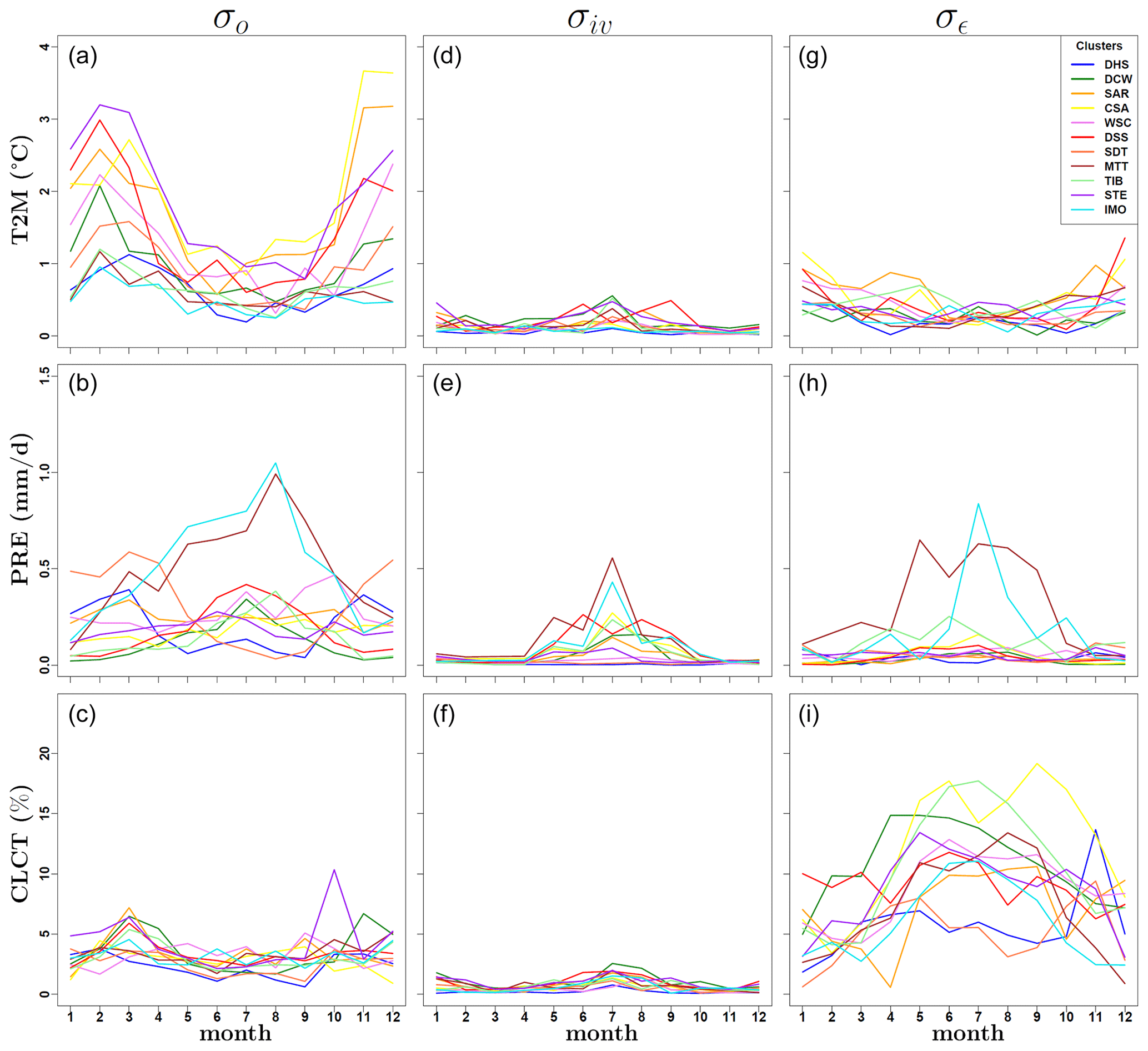
Figure 8Values of different uncertainty terms for each cluster and month used in the PI calculations. From top to bottom, the different variables are considered, in the following order: near-surface temperature (T2M), daily precipitation (PRE) and total cloud cover (CLCT). Panels (a–c) represent the uncertainties of the observation interannual variability (σo) calculated over the period of 1996–2005. In panels (d–f), the values of the model internal variability (σiv), calculated over the same period, are shown. In panels (g–i), the errors calculated over the different observational data sets, for the selected year (2000), are illustrated (σϵ).
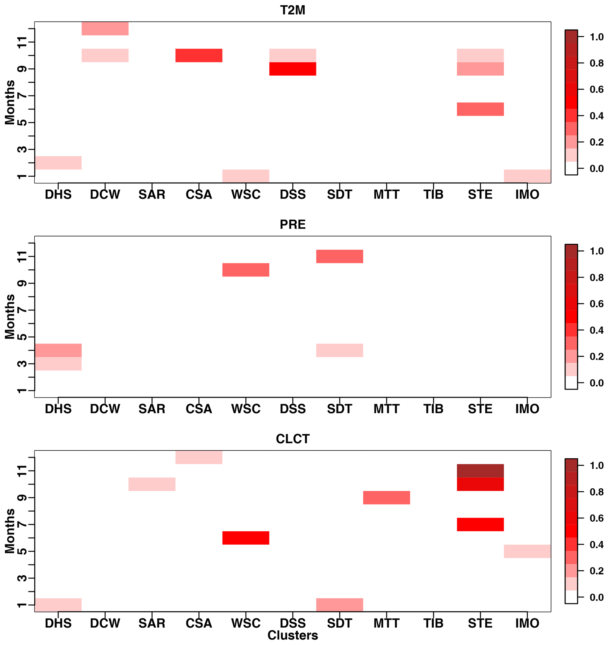
Figure 9Effects of the sum of the different uncertainty sources in the calculation of PI for each cluster and considered month, with respect to the reference model bias against observations. The error terms are firstly divided by the bias of the reference simulation for each subregion and month. Then, the values obtained for all variables are standardized between a minimum and a maximum.
Figure 9 shows the effect of the sum of the different uncertainty terms on the calculation of PI for each month and cluster, relatively to the corresponding model bias against observations. The presented values are obtained by standardizing the value of the uncertainty ∕ bias ratios, for all variables, with respect to their absolute minimum and maximum values. From this figure, it is possible to see that for the calculation of PI, uncertainties have a greater weight for T2M and CLCT than for PRE. This suggests that the lower PS values obtained for PRE are mainly due to large model biases, which in this case are completely out of the range of the corresponding uncertainties. Additionally, the same figure shows that even though the effects of the uncertainties on PI are sometimes remarkable, this is true only for given clusters and at specific months. Mostly, even if large uncertainties are present (Fig. 8), these are relatively small when compared to the corresponding model biases (one example is the case of T2M for Western Siberia during winter months in Fig. 9). In these cases, small changes in PI obtained by perturbing parameter values are indicative of small reductions of the model bias against observations and of a possible problem in the model structural formulation.
3.4 Transferability of the model configuration
In order to test whether COSMO-CLM responds similarly to parameters perturbation for different domains, the same PS analyses are conducted on a subset of model parameters for the European CORDEX domain. The same 1-year simulations for the year 2000 are conducted for the parameters e_surf, rlam_heat, rat_sea and entr_sc, using the same default configuration of the Central Asia simulations. The first two parameters are selected since they present a high sensitivity for the Central Asia domain, while the others produce almost the same results over a large part of the region for different input values. As before, a k-means clustering technique is used for dividing the European domain into subregions characterized by different climatic conditions. For having an approximately equal ratio between the total number of points and clusters as for Central Asia, six clusters are selected. Results of the clustering for Europe are shown in Fig. 10.
The PS calculated for the given parameter values for Europe and Central Asia, considering T2M, PRE and CLCT together, is presented in Fig. 11, respectively, in the left and right columns. The results show that the model has the same sensitivity over Europe and Central Asia for e_ surf, with worse performance for higher parameter values. Conversely, a different behaviour is obtained in the two cases for the other parameters. In particular, the model shows for Europe a decreasing response to an increase in parameter values for rlam_heat, differently to the Central Asia case. At the same time, for Europe, rat_sea and entr_sc present appreciable changes, in particular the first one, conversely to the Central Asia example. One important aspect to be mentioned is the fact that the values of PS calculated for Europe are higher than the ones for Central Asia. An additional analysis of the uncertainty for Europe indicates that this difference is dictated by larger model biases against observations for Central Asia, since the ranges of the uncertainties are comparable in the two cases (see the Supplement). Even though the presented analyses are conducted on a subsample of parameters, the results allow us to affirm that the model responds differently to different parameter values over Europe and Central Asia, two regions characterized by various climate conditions. This is in contrast with the recent findings of Bellprat et al. (2016), asserting that uncertainties in the model physics are common among different regions. Even though additional research on other regions is required, the presented results suggest that model calibration remains a necessary condition prior to the application of COSMO-CLM to different domains of study.
In this paper, the parameter space of the COSMO-CLM RCM is investigated for the Central Asia CORDEX domain, using a PPE obtained by performing 1-year simulations with different parameter values. The results of these simulations are compared against observations, using the performance metrics introduced in Bellprat et al. (2012a). The main goal of the paper is to characterize model parameter uncertainty, determining the most sensitive parameters for the region, on which to apply the objective calibration method of Bellprat et al. (2012b). Moreover, the presented experiments are used to investigate the effect of several parameters on the simulation of the considered variables for subregions with different climate conditions, assessing to which degree it is possible to improve model performance by properly selecting parameter values in each case. Finally, the paper explores the possibility of transferring an RCM model setup used for one region to a different domain of study.
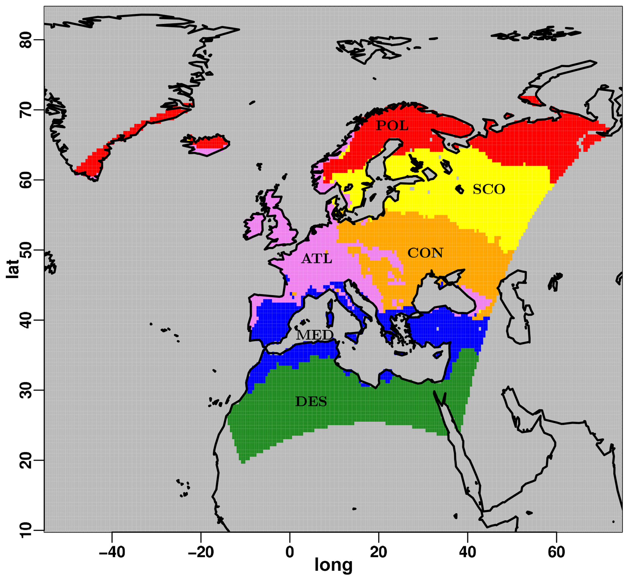
Figure 10Map of the six subregions obtained for Europe through k-means clustering of the q-normalized monthly climatologies of the considered variables, calculated over the period of 1996–2005.
The model is particularly sensitive to a subset of all the tested parameters. The parameters with the largest effect on model performance are qi0, the cloud ice threshold for autoconversion, and e_surf, the exponent to get the effective surface area. Another particularly important parameter for the area and all considered variables is rlam_heat, the scaling factor of the laminar boundary layer for heat. In addition to these three, six other most sensitive parameters are individuated: d_mom, the factor for turbulent momentum dissipation, v0snow, controlling the fall velocity of snow, radfac, which represents the fraction of cloud water/ice used in the radiation scheme, tkhmin, the minimum value for the turbulence heat diffusion coefficient, soilhyd, a multiplying factor for soil hydraulic conductivity and diffusivity, and uc1, the parameter for computing the amount of cloud cover in saturated conditions.
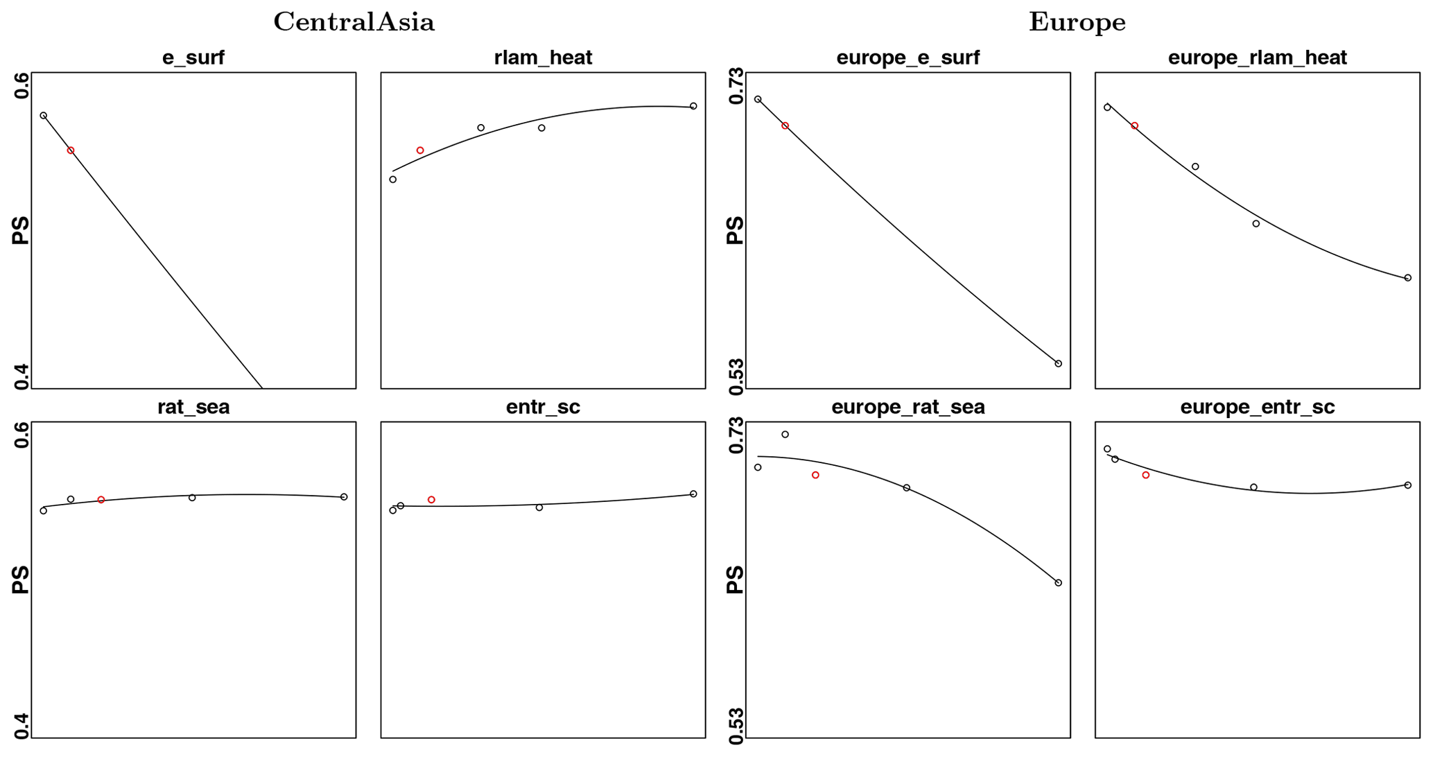
Figure 11PS values calculated for Central Asia (left) and Europe (right), for different values of the parameters e_surf, rlam_heat, rat_sea and entr_sc. The values of the parameters are the same in the two cases. Red dots correspond to the PS values obtained for the default simulation.
In general, the presented results show that an overall improvement of model performance relatively to the selected variables seems possible, by properly selecting parameter values. Nevertheless, this improvement would not be coherent among all the Central Asia domain subregions but the result of some compensating effect. The model response to parameter value perturbation is characterized by contrasting results in the different cases. The most important example in this sense is the one of qi0, producing large contrasting changes in model performance over different regions and variables. It is of crucial importance to determine a proper input for qi0 for the region, since even a small perturbation of its value could have a tremendous effect on model results, with an improvement in the performance over one region and variable, and an opposite response for others. The same is particularly true also for the parameter e_surf.
Parameters related to soil–atmosphere and land surface–atmosphere interaction representations, such as rlam_heat and soilhyd, are notably relevant for the simulation of near-surface temperature over a large part of the domain subregions, in particular over Western Siberia and the area north of the Black Sea. Nevertheless, the same parameters do not have the same influence on the simulation of precipitation and total cloud cover for the majority of the subdomains. Parameters used in the turbulence parameterization scheme, such as tkhmin, have an important impact on many regions, in particular for near-surface temperature and cloud cover, for areas characterized by complex topography and the ones with stable vertical stratification. In the latter case, tkhmin produces opposite results for the considered variables, confirming an already known model structural problem related to the production of excessive mixing over these regions. Among the parameters employed in the radiation process representations, uc1 shows a strong sensitivity, in particular for total cloud cover, over all the domain subregions. Over some subregions (e.g. Turkey and the northern part of Iran), parameters related to ocean-surface processes, such as rat_sea and c_sea, have a relevant effect on the simulation of precipitation. For some regions, such as Western Siberia, even though changes in model results are possible by perturbing parameter values, they do not seem to be large enough in order to sensibly improve model biases. In this case, the reason for the biases is most likely related to some structural error in the model formulation. However, it is worth mentioning that additional factors that were not acknowledged in this study, such as changes in the default model setup (e.g. model spatial resolution and number of vertical levels) could also affect model performance over different parts of the domain.
For the calculation of the considered metrics, a larger role is played by the uncertainties in near-surface temperature and cloud cover than the ones in precipitation. For cloud cover, the contribution of the observational uncertainties is larger than the one arising from the observational interannual and model internal variability, more important for the other two variables. The bias between model and observational data sets is particularly large for precipitation, well out of the range of considered uncertainty sources, leading to lower values of the PS with respect to the other two cases.
Finally, the model parameters' sensitivity for the Central Asia CORDEX domain does not coincide, for a selected subsample of parameters, with the one evinced for the corresponding European domain, characterized by different climatic conditions. Even though additional research on other regions is required, the presented results suggest that model calibration remains a necessary condition prior to the application of COSMO-CLM to different domains of study, contrary to evidence from recent studies using the same model. Our results suggest that a regional climate model should be retuned when setting up model experiments to a non-native domain.
Simulation configuration files can be downloaded from https://doi.org/10.5281/zenodo.3523177 (Russo, 2019a).
All the data on which the presented analyses are conducted, together with the restart files of the reference simulations used to drive the sensitivity experiments for the two domains, are available at the following link: https://doi.org/10.5281/zenodo.3523243 (Russo, 2019b).
A complete documentation of the COSMO model is permanently available at the following link: https://www.dwd.de/EN/ourservices/cosmo_documentation/cosmo_documentation.html (last access: 1 October 2020).
The COSMO-CLM model is completely free of charge for all research applications. The version of the COSMO-CLM model used in this study can be downloaded from the following website: https://redc.clm-community.eu/projects/cclm-sp/wiki/Downloads (Rockel et al., 2008).
Access is license-restricted (http://www.cosmo-model.org/content/consortium/licencing.htm, last access: 1 December 2019) and for the download the user needs to become a member of the CLM community, or the respective institute needs to hold an institutional license.
The supplement related to this article is available online at: https://doi.org/10.5194/gmd-13-5779-2020-supplement.
The simulations of this research were performed by ER. All the authors contributed to the discussion of the results, with ER and SS playing the major role. The paper structure as well as most of the presented experiments were designed by ER, with the support of SS and CR. All authors gave a substantial contribution to the revision of the text and to the formatting of the paper.
The authors declare that they have no conflict of interest.
This study was funded by the Federal Ministry of Education and Research of Germany (BMBF) as part of the CAME II project (Central Asia: Climatic Tipping Points & Their Consequences), project no. 03G0863G.
The computational resources necessary for conducting the experiments presented in this research were made available by the German Climate Computing Center (DKRZ).
The authors are also particularly grateful to the COSMO and the CLM community for all their efforts in developing the COSMO-CLM model and making its code available.
Finally, a special acknowledgement goes to Uli Schättler, Daniel Rieger and their collaborators from the German Weather Service (DWD) for making the COSMO model documentation permanently available.
This research has been supported by the Bundesministerium für Bildung und Forschung (grant no. 03G0863G).
This paper was edited by Astrid Kerkweg and reviewed by Andreas Dobler and one anonymous referee.
Annan, J. and Hargreaves, J.: Efficient estimation and ensemble generation in climate modelling, Philos. T. R. Soc. A, 365, 2077–2088, 2007. a
Annan, J. D., Lunt, D. J., Hargreaves, J. C., and Valdes, P. J.: Parameter estimation in an atmospheric GCM using the Ensemble Kalman Filter, Nonlin. Processes Geophys., 12, 363–371, https://doi.org/10.5194/npg-12-363-2005, 2005. a
Baldauf, M., Seifert, A., Förstner, J., Majewski, D., Raschendorfer, M., and Reinhardt, T.: Operational convective-scale numerical weather prediction with the COSMO model: Description and sensitivities, Mon. Weather Rev., 139, 3887–3905, 2011. a
Ball, G. and Hall Dj, I.: A novel method of data analysis and pattern classification. Isodata, A novel method of data analysis and pattern classification, Tech. Report 5RI, Project 5533, 1965. a
Ban, N., Schmidli, J., and Schär, C.: Heavy precipitation in a changing climate: Does short-term summer precipitation increase faster?, Geophys. Res. Lett., 42, 1165–1172, 2015. a
Becker, A., Finger, P., Meyer-Christoffer, A., Rudolf, B., and Ziese, M.: GPCC full data reanalysis version 7.0 at 0.5: Monthly land-surface precipitation from rain-gauges built on GTS-based and historic data, 2011. a
Bellprat, O.: Parameter uncertainty and calibration of regional climate models, PhD thesis, ETH Zurich, 2013. a, b
Bellprat, O., Kotlarski, S., Lüthi, D., and Schär, C.: Exploring perturbed physics ensembles in a regional climate model, J. Climate, 25, 4582–4599, 2012a. a, b, c, d, e, f, g, h, i, j, k, l, m
Bellprat, O., Kotlarski, S., Lüthi, D., and Schär, C.: Objective calibration of regional climate models, J. Geophys. Res.-Atmos., 117, D23115, https://doi.org/10.1029/2012JD018262, 2012b. a, b, c, d, e, f, g, h, i, j, k, l, m, n
Bellprat, O., Kotlarski, S., Lüthi, D., De Elía, R., Frigon, A., Laprise, R., and Schär, C.: Objective calibration of regional climate models: application over Europe and North America, J. Climate, 29, 819–838, 2016. a, b, c, d, e
Beltran, C., Edwards, N., Haurie, A., Vial, J., and Zachary, D.: Oracle-based optimization applied to climate model calibration, Environ. Model. Assess., 11, 31–43, 2006. a
Brisson, E., Demuzere, M., and van Lipzig, N.: Modelling strategies for performing convection-permitting climate simulations, Meteorol. Z, 25, 149–163, 2015. a
Bucchignani, E., Montesarchio, M., Cattaneo, L., Manzi, M., and Mercogliano, P.: Regional climate modeling over China with COSMO-CLM: Performance assessment and climate projections, J. Geophys. Res.-Atmos., 119, 12–151, 2014. a
Bucchignani, E., Montesarchio, M., Zollo, A., and Mercogliano, P.: High-resolution climate simulations with COSMO-CLM over Italy: performance evaluation and climate projections for the 21st century, Int. J. Climatol., 36, 735–756, 2016. a
Buzzi, M., Rotach, M., Holtslag, M., and Holtslag, A.: Evaluation of the COSMO-SC turbulence scheme in a shear-driven stable boundary layer, Meteorol. Z., 20, 335–350, 2011. a
Carlsson, B., Papadimitrakis, Y., and Rutgersson, A.: Evaluation of a roughness length model and sea surface properties with data from the Baltic Sea, J. Phys. Oceanogr., 40, 2007–2024, 2010. a
Cerenzia, I., Tampieri, F., and Tesini, M.: Diagnosis of turbulence schema in stable atmospheric conditions and sensitivity tests, Cosmo Newsletter, 14, 1–11, 2014. a
Collins, M., AchutaRao, K., Ashok, K., Bhandari, S., Mitra, A., Prakash, S., Srivastava, R., and Turner, A.: Observational challenges in evaluating climate models, Nat. Clim. Change, 3, 940–941, 2013. a
Dobler, A. and Ahrens, B.: Four climate change scenarios for the Indian summer monsoon by the regional climate model COSMO-CLM, J. Geophys. Res.-Atmos., 116, D24104, https://doi.org/10.1029/2011JD016329, 2011. a
Doms, G. and Baldauf, M.: A Description of the Nonhydrostatic Regional COSMO-Model – Part I: Dynamics and Numerics, Tech. rep., COSMO – Consortium for Small-Scale Modelling, https://doi.org/10.5676/DWD_pub/nwv/cosmo-doc_5.00_I, 2013. a
Doms, G., Föster, J., Heise, E., Herzog, H., Mironov, D., Raschendorfer, M., Reinhardt, T., Ritter, B., Schrodin, R., Schulz, J., and Vogel, G.: A Description of the Nonhydrostatic Regional COSMO-Model – Part II: Physical Parameterizations, Tech. rep., COSMO – Consortium for Small-Scale Modelling, https://doi.org/10.5676/DWD_pub/nwv/cosmo-doc_5.00_II, 2013. a
Dosio, A. and Panitz, H.-J.: Climate change projections for CORDEX-Africa with COSMO-CLM regional climate model and differences with the driving global climate models, Clim. Dynam., 46, 1599–1625, 2016. a
Dosio, A., Panitz, H.-J., Schubert-Frisius., M., and Lüthi, D.: Dynamical downscaling of CMIP5 global circulation models over CORDEX-Africa with COSMO-CLM: evaluation over the present climate and analysis of the added value, Clim. Dynam., 44, 2637–2661, 2015. a
Fallah, B., Sodoudi, S., Russo, E., Kirchner, I., and Cubasch, U.: Towards modeling the regional rainfall changes over Iran due to the climate forcing of the past 6000 years, Quatern. Int., 429, 119–128, 2015. a
Fallah, B., Sodoudi, S., and Cubasch, U.: Westerly jet stream and past millennium climate change in Arid Central Asia simulated by COSMO-CLM model, Theor. Appl. Climatol., 124, 1079–1088, 2016. a
Fernández, J., Sáenz, J., and Zorita, E.: Analysis of wintertime atmospheric moisture transport and its variability over southern Europe in the NCEP Reanalyses, Clim. Res., 23, 195–215, 2003. a
Fischer, T., Menz, C., Su, B., and Scholten, T.: Simulated and projected climate extremes in the Zhujiang River Basin, South China, using the regional climate model COSMO-CLM, Int. J. Climatol., 33, 2988–3001, 2013. a
Flaounas, E., Drobinski, P., Borga, M., Calvet, J., Delrieu, G., Morin, E., Tartari, G., and Toffolon, R.: Assessment of gridded observations used for climate model validation in the Mediterranean region: the HyMeX and MED-CORDEX framework, Environ. Res. Lett., 7, 024017, https://doi.org/10.1088/1748-9326/7/2/024017, 2012. a
Foley, A.: Uncertainty in regional climate modelling: A review, Prog. Phys. Geog., 34, 647–670, 2010. a
Fosser, G., Khodayar, S., and Berg, P.: Benefit of convection permitting climate model simulations in the representation of convective precipitation, Clim. Dynam., 44, 45–60, 2015. a
Gelaro, R., McCarty, W., Suárez, M. J., Todling, R., Molod, A., Takacs, L., Randles, C. A., Darmenov, A., Bosilovich, M. G., Wargan, R. R. K., Coy, L., Cullather, R., Draper, C., Akella, S., Buchard, V., Conaty, A., da Silva, A. M., Gu, W., Kim, G.-K., Koster, R., Lucchesi, R., Merkova, D., Nielsen, J. E., Partyka, G., Pawson, S., Putman, W., Rienecker, M., Schubert, S. D., Sienkiewicz, M., and Zhao, B.: The modern-era retrospective analysis for research and applications, version 2 (MERRA-2), J. Climate, 30, 5419–5454, 2017. a
Giorgi, F., Jones, C., and Asrar, G.: Addressing climate information needs at the regional level: the CORDEX framework, World Meteorological Organization (WMO) Bulletin, 58, 175–183, 2009. a
Gómez-Navarro, J., Montávez, J., Jerez, S., Jiménez-Guerrero, P., and Zorita, E.: What is the role of the observational dataset in the evaluation and scoring of climate models?, Geophys. Res. Lett., 39, L24701, https://doi.org/10.1029/2012GL054206, 2012. a
Gregoire, L., Valdes, P., Payne, A., and Kahana, R.: Optimal tuning of a GCM using modern and glacial constraints, Clim. Dynam., 37, 705–719, 2011. a
Gutowski Jr., W. J., Giorgi, F., Timbal, B., Frigon, A., Jacob, D., Kang, H.-S., Raghavan, K., Lee, B., Lennard, C., Nikulin, G., O'Rourke, E., Rixen, M., Solman, S., Stephenson, T., and Tangang, F.: WCRP COordinated Regional Downscaling EXperiment (CORDEX): a diagnostic MIP for CMIP6, Geosci. Model Dev., 9, 4087–4095, https://doi.org/10.5194/gmd-9-4087-2016, 2016. a
Harris, I. and Jones, P.: CRU TS4.01: Climatic Research Unit (CRU) Time-Series (TS) version 4.01 of high-resolution gridded data of month-by-month variation in climate (Jan. 1901–Dec. 2016), available at: http://catalogue.ceda.ac.uk/uuid/58a8802721c94c66ae45c3baa4d814d0 (last access: 1 February 2020), 2017. a
Hastings, D., Dunbar, P., Elphingstone, G., Bootz, M., Murakami, H., Maruyama, H., Masaharu, H., Holland, P., Payne, J., Bryant, N., Logan, T. L., Muller, J.-P., Schreier, G., and MacDonald, J. S.: The global land one-kilometer base elevation (GLOBE) digital elevation model, Version 1.0. National Oceanic and Atmospheric Administration, National Geophysical Data Center, 325 Broadway, Boulder, Colorado 80303, USA, 1999. a
Hourdin, F., Mauritsen, T., Gettelman, A., Golaz, J. C., Balaji, V., Duan, Q., Folini, D., Ji, D., Klocke, D., Qian, Y., Rauser, F., Rio, C.,; Tomassini, L., Watanabe, M., and Williamson, D.: The art and science of climate model tuning, B. Am. Meteorol. Soc., 98, 589–602, 2017. a, b, c, d, e, f
Jackson, C., Sen, M., and Stoffa, P.: An efficient stochastic Bayesian approach to optimal parameter and uncertainty estimation for climate model predictions, J. Climate, 17, 2828–2841, 2004. a
Jacob, D., Bärring, L., Christensen, O., Christensen, J., De Castro, M., Deque, M., Giorgi, F., Hagemann, S., Hirschi, M., Jones, R., Kjellström, E., Lenderink, G., Rockel, B., Sánchez, E., Schär, C., Seneviratne, S. I., Somot, S., van Ulden, A., and van den Hurk, B.: An inter-comparison of regional climate models for Europe: model performance in present-day climate, Climatic Change, 81, 31–52, 2007. a
Jacob, D., Elizalde, A., Haensler, A., Hagemann, S., Kumar, P., Podzun, R., Rechid, D., Remedio, A., Saeed, F., Sieck, K., Teichmann, C., and Wilhelm, C.: Assessing the transferability of the regional climate model REMO to different coordinated regional climate downscaling experiment (CORDEX) regions, Atmosphere, 3, 181–199, 2012. a
Jain, A. K.: Data clustering: 50 years beyond K-means, Pattern Recogn. Lett., 31, 651–666, 2010. a
Järvinen, H., Räisänen, P., Laine, M., Tamminen, J., Ilin, A., Oja, E., Solonen, A., and Haario, H.: Estimation of ECHAM5 climate model closure parameters with adaptive MCMC, Atmos. Chem. Phys., 10, 9993–10002, https://doi.org/10.5194/acp-10-9993-2010, 2010. a
Jones, C., Gregory, J., Thorpe, R., Cox, P., Murphy, J., Sexton, D., and Valdes, P.: Systematic optimisation and climate simulation of FAMOUS, a fast version of HadCM3, Clim. Dynam., 25, 189–204, 2005. a
Kanamitsu, M., Ebisuzaki, W., Woollen, J., Yang, S., Hnilo, J., Fiorino, M., and Potter, G.: Ncep–doe amip-ii reanalysis (r-2), B. Am. Meteorol. Soc., 83, 1631–1643, 2002. a
Keuler, K., Radtke, K., Kotlarski, S., and Lüthi, D.: Regional climate change over Europe in COSMO-CLM: Influence of emission scenario and driving global model, Meteorol. Z., 25, 121–136, 2016. a
Knote, C., Heinemann, G., and Rockel, B.: Changes in weather extremes: Assessment of return values using high resolution climate simulations at convection-resolving scale, Meteorol. Z., 19, 11–23, 2010. a
Knutti, R., Stocker, T., Joos, F., and Plattner, G.: Constraints on radiative forcing and future climate change from observations and climate model ensembles, Nature, 416, 719–723, https://doi.org/10.1038/416719a, 2002. a
Knutti, R., Stocker, T., Joos, F., and Plattner, G.: Probabilistic climate change projections using neural networks, Clim. Dynam., 21, 257–272, 2003. a
Lange, S., Rockel, B., Volkholz, J., and Bookhagen, B.: Regional climate model sensitivities to parametrizations of convection and non-precipitating subgrid-scale clouds over South America, Clim. Dynam., 44, 2839–2857, 2015. a
Lempert, R., Nakicenovic, N., Sarewitz, D., and Schlesinger, M.: Characterizing climate-change uncertainties for decision-makers. An editorial essay, Climatic Change, 65, 1–9, 2004. a
Lloyd, S.: Least squares quantization in PCM, IEEE T. Inform. Theory, 28, 129–137, 1982. a
MacQueen, J.: Some methods for classification and analysis of multivariate observations, in: Proceedings of the fifth Berkeley symposium on mathematical statistics and probability, Oakland, CA, USA, vol. 1, 281–297, 1967. a
Mannig, B., Müller, M., Starke, E., Merkenschlager, C., Mao, W., Zhi, X., Podzun, R., Jacob, D., and Paeth, H.: Dynamical downscaling of climate change in Central Asia, Global Planet. Change, 110, 26–39, 2013. a
Medvigy, D., Walko, R., Otte, M., and Avissar, R.: The Ocean–Land–Atmosphere Model: Optimization and evaluation of simulated radiative fluxes and precipitation, Mon. Weather Rev., 138, 1923–1939, 2010. a
Meng, X., Lyu, S., Zhang, T., Zhao, L., Li, Z., Han, B., Li, S., Ma, D., Chen, H., Ao, Y., Luo, S., Shen, Y, Guo, J., and Wen, L.: Simulated cold bias being improved by using MODIS time-varying albedo in the Tibetan Plateau in WRF model, Environ. Res. Lett., 13, 044028, https://doi.org/10.1088/1748-9326/aab44a, 2018. a
Murphy, J., Booth, B., Collins, M., Harris, G., Sexton, D., and Webb, M.: A methodology for probabilistic predictions of regional climate change from perturbed physics ensembles, Philos. T. R. Soc. A, 365, 1993–2028, 2007. a
Murphy, J. M., Sexton, D. M., Barnett, D. N., Jones, G. S., Webb, M. J., Collins, M., and Stainforth, D. A.: Quantification of modelling uncertainties in a large ensemble of climate change simulations, Nature, 430, 768–772, https://doi.org/10.1038/nature02771, 2004. a, b
Neelin, J., Bracco, A., Luo, H., McWilliams, J., and Meyerson, J.: Considerations for parameter optimization and sensitivity in climate models, P. Natl. Acad. Sci. USA, 107, 21349–21354, 2010. a, b
O'Hagan, A.: Bayesian analysis of computer code outputs: A tutorial, Reliab. Eng. Syst. Safe., 91, 1290–1300, 2006. a
Ollinaho, P., Laine, M., Solonen, A., Haario, H., and Järvinen, H.: NWP model forecast skill optimization via closure parameter variations, Q. J. Roy. Meteor. Soc., 139, 1520–1532, 2013. a
Ozturk, T., Altinsoy, H., Türkeş, M., and Kurnaz, M.: Simulation of temperature and precipitation climatology for the Central Asia CORDEX domain using RegCM 4.0, Clim. Res., 52, 63–76, 2012. a
Ozturk, T., Turp, M., Türkeş, M., and Kurnaz, M.: Projected changes in temperature and precipitation climatology of Central Asia CORDEX Region 8 by using RegCM4. 3.5, Atmos. Res., 183, 296–307, 2017. a
Paeth, H.: Insights from large ensembles with perturbed physics, Erdkunde, 69, 201–216, 2015. a, b, c
Paeth, H., Steger, C., and Merkenschlager, C.: Climate Change – it's All About Probability, Erdkunde, 67, 203–222, 2013. a
Price, A., Myerscough, R., Voutchkov, I., Marsh, R., and Cox, S.: Multi-objective optimization of GENIE Earth system models, Philos. T. R. Soc. A, 367, 2623–2633, 2009. a
Prömmel, K., Cubasch, U., and Kaspar, F.: A regional climate model study of the impact of tectonic and orbital forcing on African precipitation and vegetation, Palaeogeogr. Palaeocl., 369, 154–162, 2013. a
Rockel, B. and Geyer, B.: The performance of the regional climate model CLM in different climate regions, based on the example of precipitation, Meteorol. Z., 17, 487–498, 2008. a
Rockel, B., Will, A., and Hense, A.: Regional climate modelling with COSMO-CLM (CCLM), Meteorol. Z., 17, 347–348, 2008. a, b, c
Russo, E.: COSMO-CLM Namelists for the simulations exploring the model parameter space over the CORDEX Central Asia domain, Zenodo, https://doi.org/10.5281/zenodo.3523177, 2019a. a
Russo, E.: CCLM outputs Parameters Sensitivity Investigation Central Asia and Europe [Data set], Zenodo, https://doi.org/10.5281/zenodo.3523243, 2019b. a
Russo, E. and Cubasch, U.: Mid-to-late Holocene temperature evolution and atmospheric dynamics over Europe in regional model simulations, Clim. Past, 12, 1645–1662, https://doi.org/10.5194/cp-12-1645-2016, 2016. a
Russo, E., Kirchner, I., Pfahl, S., Schaap, M., and Cubasch, U.: Sensitivity studies with the regional climate model COSMO-CLM 5.0 over the CORDEX Central Asia Domain, Geosci. Model Dev., 12, 5229–5249, https://doi.org/10.5194/gmd-12-5229-2019, 2019. a, b, c, d, e, f, g, h, i, j
Schirber, S., Klocke, D., Pincus, R., Quaas, J., and Anderson, J.: Parameter estimation using data assimilation in an atmospheric general circulation model: From a perfect toward the real world, J. Adv. Model. Earth Sy., 5, 58–70, 2013. a
Solman, S., Sanchez, E., Samuelsson, P., da Rocha, R., Li, L., Marengo, J., Pessacg, N., Remedio, A., Chou, S., Berbery, H., Le Treut, H., de Castro, M., and Jacob, D.: Evaluation of an ensemble of regional climate model simulations over South America driven by the ERA-Interim reanalysis: model performance and uncertainties, Clim. Dynam., 41, 1139–1157, 2013. a
Sørland, S., Schär, C., Lüthi, D., and Kjellström, E.: Bias patterns and climate change signals in GCM-RCM model chains, Environ. Res. Lett., 13, 074017, https://doi.org/10.1088/1748-9326/aacc77, 2018. a
Stainforth, D. A., Aina, T., Christensen, C., Collins, M., Faull, N., Frame, D. J., Kettleborough, J. A., Knight, S., Martin, A., Murphy, J. M., Piani, C., Sexton, D., Smith, L. A., Spicer, R. A., Thorpe, A. J., and Allen M. R.: Uncertainty in predictions of the climate response to rising levels of greenhouse gases, Nature, 433, 403–406, https://doi.org/10.1038/nature03301, 2005. a
Steinhaus, H.: Sur la division des corp materiels en parties, B. Acad. Pol. Sci., 1, 801–804, 1956. a
Takle, E. S., Roads, J., Rockel, B., Gutowski, W. J., Arritt, R. W., Meinke, I., Jones, C. G., and Zadra, A.: Transferability intercomparison: an opportunity for new insight on the global water cycle and energy budget, B. Am. Meteorol. Soc., 88, 375–384, 2007. a
Tebaldi, C. and Knutti, R.: The use of the multi-model ensemble in probabilistic climate projections, Philos. T. R. Soc. A, 365, 2053–2075, 2007. a, b, c
Tegen, I., Hollrig, P., Chin, M., Fung, I., Jacob, D., and Penner, J.: Contribution of different aerosol species to the global aerosol extinction optical thickness: Estimates from model results, J. Geophys. Res.-Atmos., 102, 23895–23915, 1997. a
Tett, S., Mineter, M., Cartis, C., Rowlands, D., and Liu, P.: Can Top-of-Atmosphere Radiation Measurements Constrain Climate Predictions? Part I: Tuning, J. Climate, 26, 9348–9366, https://doi.org/10.1175/JCLI-D-12-00595.1, 2013. a
Thévenot, O., Bouin, M., Ducrocq, V., Brossier, C., Nuissier, O., Pianezze, J., and Duffourg, F.: Influence of the sea state on Mediterranean heavy precipitation: a case-study from HyMeX SOP1, Q. J. Roy. Meteor. Soc., 142, 377–389, 2016. a
Tölle, M., Gutjahr, O., Busch, G., and Thiele, J.: Increasing bioenergy production on arable land: Does the regional and local climate respond? Germany as a case study, J. Geophys. Res.-Atmos., 119, 2711–2724, 2014. a
Vickers, D. and Mahrt, L.: Sea-surface roughness lengths in the midlatitude coastal zone, Q. J. Roy. Meteor. Soc., 136, 1089–1093, 2010. a
Von Storch, H. and Zwiers, F.: Statistical analysis in climate research, Cambridge University Press, 2001. a
Voudouri, A., Khain, P., Carmona, I., Bellprat, O., Grazzini, F., Avgoustoglou, E., Bettems, J., and Kaufmann, P.: Objective calibration of numerical weather prediction models, Atmos. Res., 190, 128–140, 2017. a
Voudouri, A., Khain, P., Carmona, I., Avgoustoglou, E., Kaufmann, P., Grazzini, F., and Bettems, J.: Optimization of high resolution COSMO model performance over Switzerland and Northern Italy, Atmos. Res., 213, 70–85, 2018. a
Wang, D., Menz, C., Simon, T., Simmer, C., and Ohlwein, C.: Regional dynamical downscaling with CCLM over East Asia, Meteorol. Atmos. Phys., 121, 39–53, 2013. a
Williamson, D., Goldstein, M., Allison, L., Blaker, A., Challenor, P., Jackson, L., and Yamazaki, K.: History matching for exploring and reducing climate model parameter space using observations and a large perturbed physics ensemble, Clim. Dynam., 41, 1703–1729, 2013. a
Willmott, C. J.: Terrestrial air temperature and precipitation: Monthly and annual time series (1950–1996), available at: http://climate.geog.udel.edu/~climate/html_pages/README.ghcn_ts.html (last access: 1 February 2020), 2000. a
Wylie, D., Jackson, D., Menzel, W., and Bates, J.: Trends in global cloud cover in two decades of HIRS observations, J. Climate, 18, 3021–3031, 2005. a
Zhou, W., Tang, J., Wang, X., Wang, S., Niu, X., and Wang, Y.: Evaluation of regional climate simulations over the CORDEX-EA-II domain using the COSMO-CLM model, Asia-Pac. J. Atmos. Sci., 52, 107–127, 2016. a
Zhuo, H., Liu, Y., and Jin, J.: Improvement of land surface temperature simulation over the Tibetan Plateau and the associated impact on circulation in East Asia, Atmos. Sci. Lett., 17, 162–168, 2016. a