Prioritising the sources of pollution in European cities: do air quality modelling applications provide consistent responses?

To take decisions on how to improve air quality, it is useful to perform a source allocation study that identifies the main sources of pollution for the area of interest. Often source allocation is performed with a chemical transport model (CTM) but unfortunately, even if accurate, this technique is time consuming and complex. Comparing the results of different CTMs to assess the uncertainty of source allocation results is even more difficult. In this work, we compare the source allocation (for PM_2.5 yearly averages) in 150 major cities in Europe, based on the results of two CTMs (CHIMERE and EMEP), approximated with the SHERPA (Screening for High Emission Reduction Potential on Air) approach. Although contradictory results occur in some cities, the source allocation results obtained with the two SHERPA simplified models lead to similar results in most cases, even though the two CTMs use different input data and configurations.

1 Introduction

Air quality models are useful tools to perform a variety of tasks like assessment (simulating concentrations fields at a given moment), forecasting (predicting future concentrations), and source allocation and planning (evaluating priorities of interventions, and the impact of potential emission reduction policies on concentrations). For assessment (Alvaro Gomez-Losada et al., 2018) and forecasting, it is possible to compare the model results with observations. For example, FAIRMODE¹ (the Forum for Air Quality Modelling in Europe) proposes methods as the Model Quality Indicator and Model Quality Objective (Pernigotti el al., 2013b; Viaene et al., 2016) to assess the quality of the model results for a given application. However, there is no benchmark against which to compare model results for source allocation and planning, as no measurements are available to test the impact of theoretical emission reduction scenarios on concentrations. So, even if it is very useful to evaluate ex ante the impact of possible policy options, it is hard to judge the quality of these results. On the other hand, the uncertainty associated with source allocation results can be assessed by comparing them with results from other air quality models (Thunis et al., 2007; Pernigotti et al., 2013). Both the absolute and relative impacts of emission reductions can then be compared.

As an initial phase to design an air quality plan, one is interested in identifying the main sources over a given domain that are responsible for the pollution at a given location (Isakov et al., 2017). This step is defined in the literature as source allocation (Thunis et al., 2019), i.e. a technique applied to understand the key contributors to air pollution at a given location. Source allocation then serves as the cornerstone to choose the target sector or geographical area when designing measures for an air quality plan.

The ideal way to perform source allocation would be to use a chemical transport model (CTM) directly, but this technique is unfortunately too time consuming to differentiate the impacts of many sources at the same time for various cities in Europe. An alternative is to simplify the CTM with a so-called source–receptor relationship (SRR) approach, which mimics the CTM relationships between emission and concentration changes. The most precise SRR would consist of an independent grid-cell-to-grid-cell approach. While this approach would allow a high level of flexibility in defining the zones over which emissions are spatially reduced, it involves simulating independently the effect of emissions changes in each single grid cell that has pollutant emissions in the model domain. It would require changing precursor emissions in individual grid cells one at a time and looking at the resulting change in concentrations in each receptor cell. While theoretically very simple, the resulting number of unknown parameters describing the transfers between source and receptor cells that need to be identified is very large. For example, for a domain with 50 × 50 grid cells (N_grid = 2500) and 5 precursors (N_prec = 5), the identification of a maximum of 12 500 parameters would be required (if emissions occur in, and concentration changes need to be calculated for, all grid cells in the domain) to calculate the change of concentration at a given receptor cell. Therefore 12 500 equations, each connecting concentration changes and emission changes, are necessary to identify these 12 500 unknown parameters. Because each of these equations requires an independent CTM run, this independent grid-cell-to-grid-cell option is very costly, and simplifying assumptions that reduce the number of CTM runs are required (Clappier et al., 2015).

In GAINS (“Greenhouse gas – Air pollution Interactions and Synergies”; Amann et al., 2011) the grid-cell-to-grid-cell relation is simplified by aggregating source cells into countries. The number of unknown parameters that need to be identified for one receptor cell equals the number of countries (N_country) multiplied by the number of precursors. This system can only be solved if at least “N_prec × N_country” equations are available, requiring a similar number of independent CTM scenarios. In GAINS, about 50 countries and 5 precursors lead to the need for 250 independent CTM scenarios to identify 250 unknowns. However, because they are derived from emission reductions at country level, these SRRs are not applicable at the urban scale.

In the RIAT+ tool (“Regional Integrated Assessment Tool”; Carnevale et al., 2014), emissions are aggregated into “quadrants” that are defined relatively to each grid cell within the domain. The “quadrant” emissions and their related grid cell concentrations are then used to feed a neural network that delivers the SRR (Carnevale et al., 2009). Although the approach requires a limited number of full CTM simulations (around 20), the set-up of the SRR remains complex due to the need to implement sophisticated neural networks.

In SHERPA (Thunis et al., 2016; Pisoni et al., 2017), a different approach is taken that reproduces the grid-cell-to-grid-cell approach but does not require anywhere near as many CTM runs. SHERPA assumes that the unknown parameters vary on a cell-by-cell basis but are no longer independent of each other. Instead, these coefficients are assumed to be related through a “bell shape function”. With the SHERPA approach, the number of unknown parameters is then equal to 2 for each precursor and receptor cell. Consequently, for the five precursors of PM_2.5 (VOC, SO₂, NO_x, PPM and NH₃), 10 independent CTM simulations are needed for a given receptor cell. Provided that they deliver independent information, the same CTM scenarios can be used to identify both parameters for all cells within the domain (see details in Pisoni et al., 2017). Based on these 10 CTM simulations the SHERPA approach allows the impact of emission reductions to be quickly assessed for many combinations of sectors, geographical areas and precursors. It is currently the only approach that allows systematic analysis to be performed for about 150 EU cities in terms of sectors and precursors.

First, the SHERPA SRR approximation of the two CTMs, CHIMERE and EMEP, is built. With these two SRR models the contribution of 100 sector–area–precursor combinations to the concentration in the city centre is determined and we assess the similarities and differences between these two sets of results. Obviously some of the differences are caused by the fact that the two CTM models rely on different formulations and parametrisations but also by the fact that they use different input data (emissions, meteorology, etc.). The objective of this work is to assess the overall uncertainty (or better, variability) attached to source allocation rather than to assess the sensitivity of the results to a given parameter (e.g. emissions).

The focus of this study is on PM_2.5 yearly averages, because this is the pollutant with the highest impact on human health and is therefore a key focus for policy-makers in Europe. Because a large number of sources contribute to PM_2.5 concentrations at one location, this is also the most challenging pollutant to manage in air quality plans.

The paper is structured as follows. We briefly present the two CTMs and their set-up in Sect. 2. We then describe the SHERPA methodology and its assumptions in Sect. 3. Section 4 details the methodology followed for the source allocation, while the inter-comparison of the results is presented in Sect. 5. Conclusions are proposed in Sect. 6.

2 CHIMERE and EMEP chemical transport models: set-up and simulations

In this work, we use two sets of model simulations, performed with two of the leading chemical transport models in Europe: CHIMERE and EMEP. More details on the models can be found in Mailler et al. (2017) and Couvidat et al. (2018) (for CHIMERE) and Simpson et al., 2012 (for EMEP). Because a brute-force source allocation for 150 cities with these models would be too time consuming, we use two sets of SHERPA SRRs, each based on a training set of about 20 CHIMERE and EMEP CTM simulations. These SRRs are then used to perform the source allocation. Details on the SHERPA training for CHIMERE can be found in Clappier et al. (2015), and for EMEP in Pisoni et al. (2019).

The CHIMERE and EMEP modelling set-ups differ in the following aspects:

• Grid setting. CHIMERE uses a grid of 0.125^∘ longitude by 0.0625^∘ latitude, corresponding to rectangular cells of more or less 9 km by 7 km (in the centre of the domain), whereas EMEP uses a regular grid of 0.1^∘ by 0.1^∘, corresponding to rectangular cells of more or less 7 km by 11 km.

• Emissions. The CHIMERE emission reference year is 2010 with a gridding based on the EC4MACS project proxies (Terrenoire et al., 2015), while EMEP uses a JRC set of emissions (Trombetti et al., 2017) based on 2014 as the reference year.

• Boundary conditions. The CHIMERE domain extends from 10.5^∘ E to 37.5^∘ W and between 34 and 62^∘ N, while the EMEP domain extends from 30^∘ E to 90^∘ W and between 30 and 82^∘ N.

• Meteorology. The two models use a different reference meteorological year: 2009 for CHIMERE and 2014 for EMEP. Both meteorological fields are modelled through the Integrated Forecasting System (IFS) of ECMWF.

• Model parameterisation. Apart from the vertical and/or horizontal resolutions, transport, deposition and chemical processes are reproduced with different levels of complexity in the two models.

Some of the validation results for the two model configurations (CHIMERE and EMEP) are briefly presented in the Supplement, showing similar performances in terms of comparison against observations. For CHIMERE the relation between predictions and observations at background stations is best characterised by a line through the origin with slope of 1.05, indicating a slight under-prediction. The standard error is 5.7 µg m⁻³ and uniform over the range of concentrations. The R² is 0.9. Concentrations at traffic and industrial stations are underestimated by roughly 10 %. For EMEP the relation between predictions and observations is best characterised by a power law with exponent 0.66. The data show a relative standard error constant over the range of concentrations and equal to 30 %. Concentrations at traffic stations are under-predicted by 9 % and over-predicted at industrial sites by 7 %. It is important to note that the use of different input and model set-ups (as listed before) represents the usual practice when air quality models are used, at the local scale, to assess the impact of air quality plans. This is why it is important here to analyse how this choice influences the results and the subsequent design of an air quality plan, an issue that is often not tackled in the literature. Finally, differences can arise from the SRR approximations themselves, even if validation against CTM simulations show similar results for the two model set-ups considered (see Supplement).

Starting from these configurations, two sets of SRRs are built for yearly average PM_2.5 concentrations, based respectively on CHIMERE and EMEP data.

Before looking at the source allocation results, in the next section a brief description of the SHERPA methodology is proposed.

3 SHERPA methodology

Starting from the simulations performed with CHIMERE and EMEP, two sets of SHERPA SRR are built. Here we briefly summarise how the SHERPA methodology works; we refer to Pisoni et al. (2019) for more details.

In the SHERPA approach, the PM concentration change in receptor cell “j” is computed as follows:

$$\begin{array}{}\text{(1)}& \mathrm{\Delta }{\mathrm{PM}}_j=\sum _p^{N_{\mathrm{prec}}}\sum _i^{N_{\mathrm{grid}}}{a}_{ij}^p\mathrm{\Delta }{E}_i^p,\end{array}$$

where N_grid is the number of grid cells within the domain, N_prec is the number of precursors, $\mathrm{\Delta }{E}_i^p$ denotes the emission changes, and $a_{ij}^p$ are the unknown parameters to be identified, representing the transfer coefficients between each source cell i and receptor cell j. In SHERPA the $a_{ij}^p$ coefficients are cell-dependent and assume a bell shape function. This bell shape function accounts for variation in terms of distance but is directionally isotropic and can be defined as follows:

$$\begin{array}{}\text{(2)}& a_{ij}^p={\mathit{\alpha }}_j^p{\left(\mathrm{1}+d_{ij}\right)}^{-{\mathit{\omega }}_j^p},\end{array}$$

where d_ij is the distance between a receptor cell “j” and a source cell “i”. Thus, in SHERPA the matrix of transfer coefficients is known when the two parameters α and ω are identified for a given receptor cell j and a given precursor p (see Eq. 2). The final formulation implemented in SHERPA is as follows:

$$\begin{array}{}\text{(3)}& \mathrm{\Delta }{\mathrm{PM}}_j=\sum _p^{N_{\mathrm{prec}}}\sum _i^{N_{\mathrm{grid}}}{\mathit{\alpha }}_j^p{\left(\mathrm{1}+d_{ij}\right)}^{-{\mathit{\omega }}_j^p}\mathrm{\Delta }{E}_i^p.\end{array}$$

With the SHERPA approach, the key step is so to find the optimal α,ω coefficients. As the number of unknown parameters is equal to 2 (α,ω) for each precursor and receptor cell “j”, for the five precursors of PM_2.5 (VOC – volatile organic compounds, SO₂ – sulfur dioxide, NO_x – nitrogen oxides, PPM – primary particulate matter and NH₃ – ammonia), 10 independent CTM simulations are needed for a given receptor cell. We refer to Pisoni et al. (2018) and Thunis et al. (2016) for additional details about the SHERPA formulation and evaluation process. Given its cell-to-cell characteristics (Eq. 3), the SHERPA formulation can be used to assess the impact of emission reductions over any given set of grid cells. Different geographical entities can therefore be freely defined in terms of boundaries.

As mentioned earlier, the SHERPA approach is used in this work to analyse the differences in source allocation results between two CTMs: CHIMERE and EMEP, referred to in this paper as S-CHIMERE and S-EMEP, respectively. The “S-“ first letter in these acronyms reminds that we compare the EMEP and CHIMERE SRRs rather than the models themselves.

4 Source allocation methodology

The aim of this work is to compare the main contributors to urban pollution in terms of sectors, geographical areas and precursors, obtained with S-CHIMERE and S-EMEP. We focus on the PM_2.5 yearly average concentrations as a target indicator, because PM_2.5 is responsible for most of the health-related burden in the EU urban areas (EEA 2019). The approach is applied to 150 European cities, those analysed in the “PM_2.5 Urban Atlas” (Thunis et al., 2018).

As mentioned above, the cell-to-cell characteristics of the SHERPA approach allow the impact of emission reductions to be assessed over any given set of grid cells (cities, regions or countries can be freely defined in terms of boundaries), and emission reductions can be freely defined in terms of precursors or sectors. The following single (or combination of) sectors, source areas and precursors are considered as sources.

In terms of sectors, the source categories follow the CORINAIR SNAP nomenclature for emissions:

• Combustion in energy and transformation industries (SNAP 1),

• Non-industrial combustion plants (SNAP 2),

• Combustion in manufacturing industry (SNAP 3),

• Production processes (SNAP 4),

• Extraction and distribution of fossil fuels and geothermal energy (SNAP 5),

• Solvent use and other product use (SNAP 6),

• Road transport (SNAP 7),

• Other mobile sources and machinery (SNAP 8),

• Waste treatment and disposal (SNAP 9) and

• Agriculture (SNAP 10),

which have been aggregated in this work into five sectors:

• industry (SNAP 1, 3 and 4),

• residential (SNAP 2),

• traffic (SNAP 7),

• agriculture (SNAP 10) and

• others (SNAP 5, 6, 8 and 9).

In terms of geographical sources, four areas are considered for the analysis:

• the core city,

• the commuting zone,

• the rest of the country and

• international (what is outside the country considered).

The commuting zone is defined as the area surrounding the city where at least 15 % of the population commutes daily to the core city. The combination of the core city and the commuting zone is referred to as the functional urban area, or FUA (see https://www.oecd.org/cfe/regional-policy/functionalurbanareasbycountry.htm, last access: 16 November 2020, for details).

Finally, the precursors considered are NO_x, VOC, NH₃, PPM and SO₂.

This leads to 100 (4 areas × 5 precursors × 5 sectors) runs for each SRR and city. For small cities (66 out of 150) the core city covers too few grid cells, which would lead to discretisation errors. In such cases, the analysis is restricted to the FUA. For these cities, 75 runs (3 areas × 5 precursors × 5 sectors) per city and model were therefore performed. With 150 analysed cities for two CTM models, we note that the SHERPA approach allows for a comparison that would have implied 26 700 (($\mathrm{66}\times \mathrm{75}+\mathrm{84}\times \mathrm{100}$) ×2 models) independent air quality simulations with a full CTM. The same amount of runs with the SHERPA simplified model only takes few seconds per scenario. The results for S-CHIMERE were published in the “Urban PM_2.5 Atlas” (Pisoni et al., 2018). In this paper, the same runs are done with S-EMEP, and a comparison between the two is provided.

Each run performed with the SHERPA SRRs provides a concentration change (ΔC) that results from an emission reduction (ΔE) with an intensity α applied to a given precursor, for a given sector and within a given area. The “relative potential” of a given precursor–sector–area source is expressed as ΔC∕αC (Thunis and Clappier, 2014). This indicator represents the share of a particular emission source to the concentration. From a policy point of view, high “relative potential” sources are the ones to be addressed first to achieve the largest improvements. In this work, the SRRs ΔC are obtained for emission reductions of α=50 %, a level that represents a threshold below which the quasi-linearity of the model responses is preserved (Thunis et al., 2015). In other words, with this approach the model response in terms of concentration change remains proportional to the emission change. It is important to stress that this threshold is only valid for PM_2.5 and for yearly average concentrations, as considered here. Because of this 50 % threshold, it is also worthwhile to note that the source allocation results discussed here provide information on the impact of potential emission reductions up to that level, not beyond.

To compare the “relative potentials” from S-CHIMERE and S-EMEP, we calculate the correlation. A high correlation means that both models agree well on the emission sources (sectoral and/or geographic) that contribute most to the concentration for a given city. The main advantage of a correlation indicator is that it ignores systematic differences. In other words, if one model systematically predicts higher concentration changes for all sources than the other, this is not detected by the correlation metric. This is a desirable characteristic because from a policy perspective, it is the “relative ranking” among the sources contributions that counts rather than their absolute values.

5 Comparison of the results

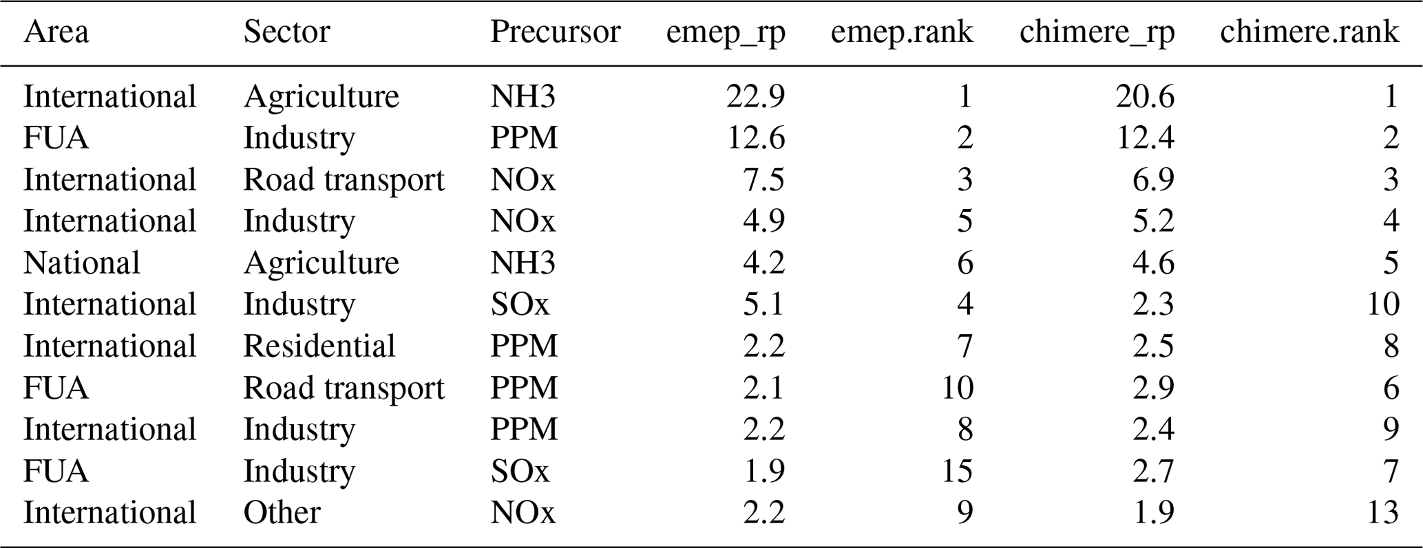
In this study, we compare the relative potentials for 150 cities, based on the two SHERPA implementations, S-CHIMERE and S-EMEP. Source allocation is calculated at the city location characterised by the worst target indicator value, i.e. the most polluted cell in the city considered. We first discuss the results for a few cities, before moving to an EU wide perspective. Tables 1 to 4 show, for each emission area, sector and precursor, the “relative potential” expressed in percentage of the total concentration for the two models (“chimere_rp” and “emep_rp”) and the resulting ranking in terms of importance (“emep.rank” and “chimere.rank”) for four cities: Liège, Genova, Turin and Madrid. These cities are selected as representative samples to illustrate the characteristic behaviours obtained in our comparison. In addition to this, Figs. 1 to 4 show the S-CHIMERE/S-EMEP correlations obtained for various relative potentials defined in terms of geographical area, sector or their combinations. For Liège (Belgium), the overall (all individual sectors, precursors and areas included, i.e. about 15 000 relative potentials) Pearson correlation² between the relative potentials of both SRRs is the highest among the 150 cities (r = 0.99; see Fig. 1). Both models identify ammonia emissions from agriculture, outside Belgium, as the main contributor to local PM_2.5 concentrations. Primary PM from local industry comes second and NO_x from international traffic third. Although the lower ranked combinations are not identical, they are quite similar. From a policy perspective, the fact that both SRRs provide similar information is a sign of robustness. It increases our confidence in the priority of interventions (which sectors and areas to act on first to achieve the maximum air quality improvement). The values for the main sector–precursor–area relative potentials are reported in Table 1.

Table 1 Top 10 area–sector–precursor relative potentials to PM_2.5 concentrations in Liège (B).

A breakdown analysis for Liège is proposed in Fig. 1, where correlations are calculated for relative potentials that are aggregated in terms of sectors (5 relative potentials), area (4 relative potentials) or area/sector (5 × 5 relative potentials). In the case of Liège, all correlations are very good.

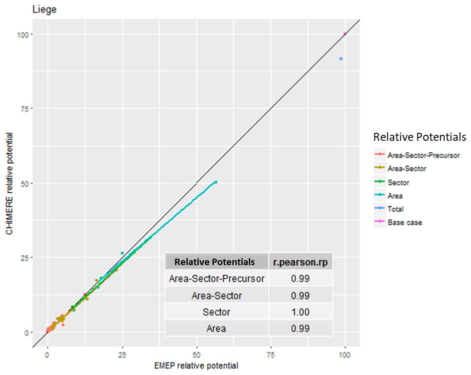
Figure 1 Correlation between S-EMEP and S-CHIMERE relative potentials for different sector–area–precursor source aggregations in Liège (B).

Unfortunately, the agreement is not always so good. For the city of Genova (Table 2 and Fig. 2), both models agree that national and international ammonia emissions from agriculture are the largest contributors to local PM_2.5 (see Table 2). But the third position in the priority ranking is occupied by NO_x from national traffic for S-EMEP while it is PPM from the national residential sector for S-CHIMERE. However, the overall correlation still reaches 89 % and the two main sources are similar. The agreement between the two models is therefore still satisfactory. It is interesting to note that for area-aggregated relative potentials, the correlation drops to 42 %, highlighting possible differences in the way emission inventories are spatially distributed in the two models.

Table 2 Top 10 area–sector–precursor relative potentials to PM_2.5 concentrations in Genova (IT).

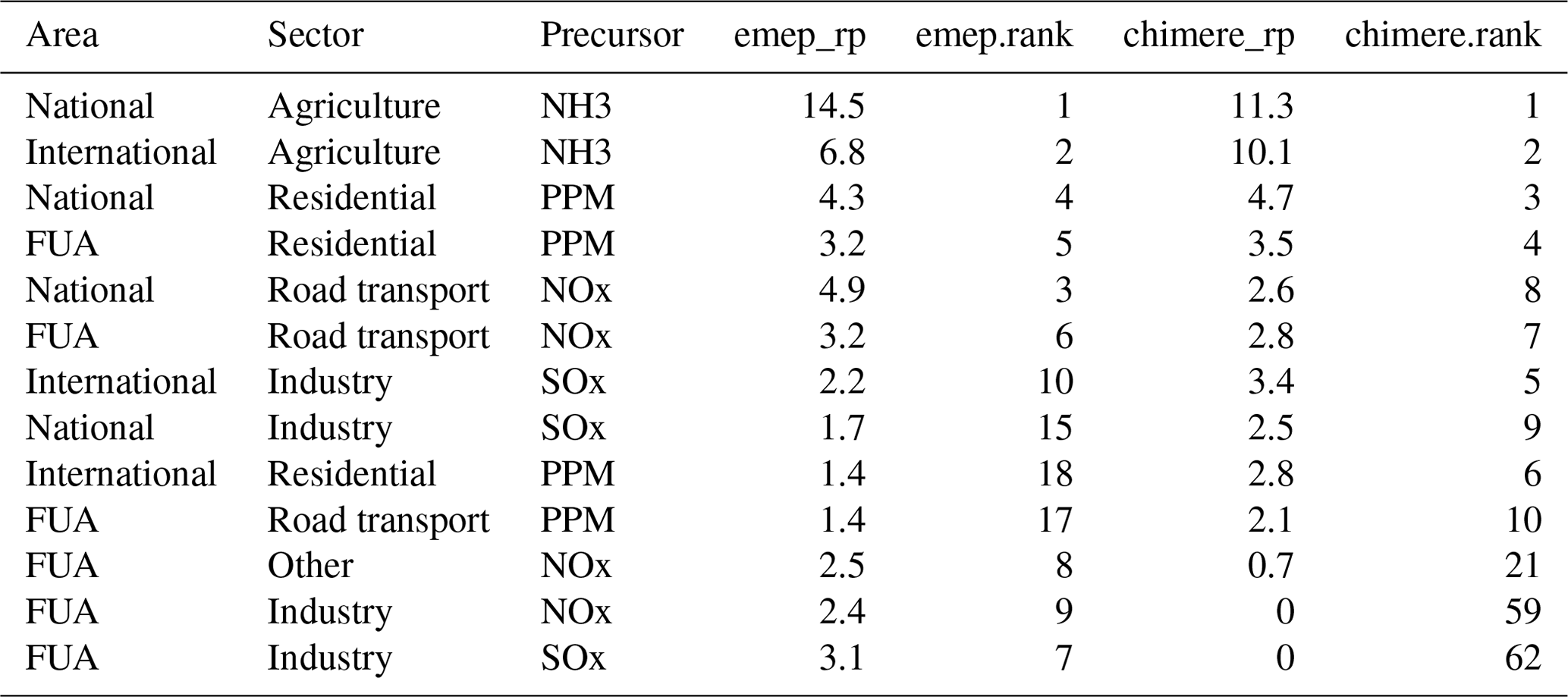
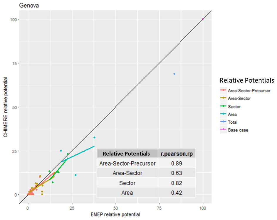
Figure 2 Correlation between S-EMEP and S-CHIMERE relative potentials for different sector–area–precursor source aggregations in Genova (I).

In the case of Torino (Table 3 and Fig. 3), the two models give contradicting recommendations. While S-CHIMERE points to city residential heating as the main contributor to PM_2.5, S-EMEP points to national agriculture ammonia emissions. The model disagreement extends to the top five relative potentials. As indicated, the problem is probably related to the sectoral (R² = 0.78) rather than to the geographical dimension (R² = 0.97). Nevertheless, the overall correlation (0.81) is not too bad and can be explained by the fact that the contribution values are not too different from each other (although the ranking is quite different).

Table 3 Top 10 area–sector–precursor relative potentials to PM_2.5 concentrations in Torino (I).

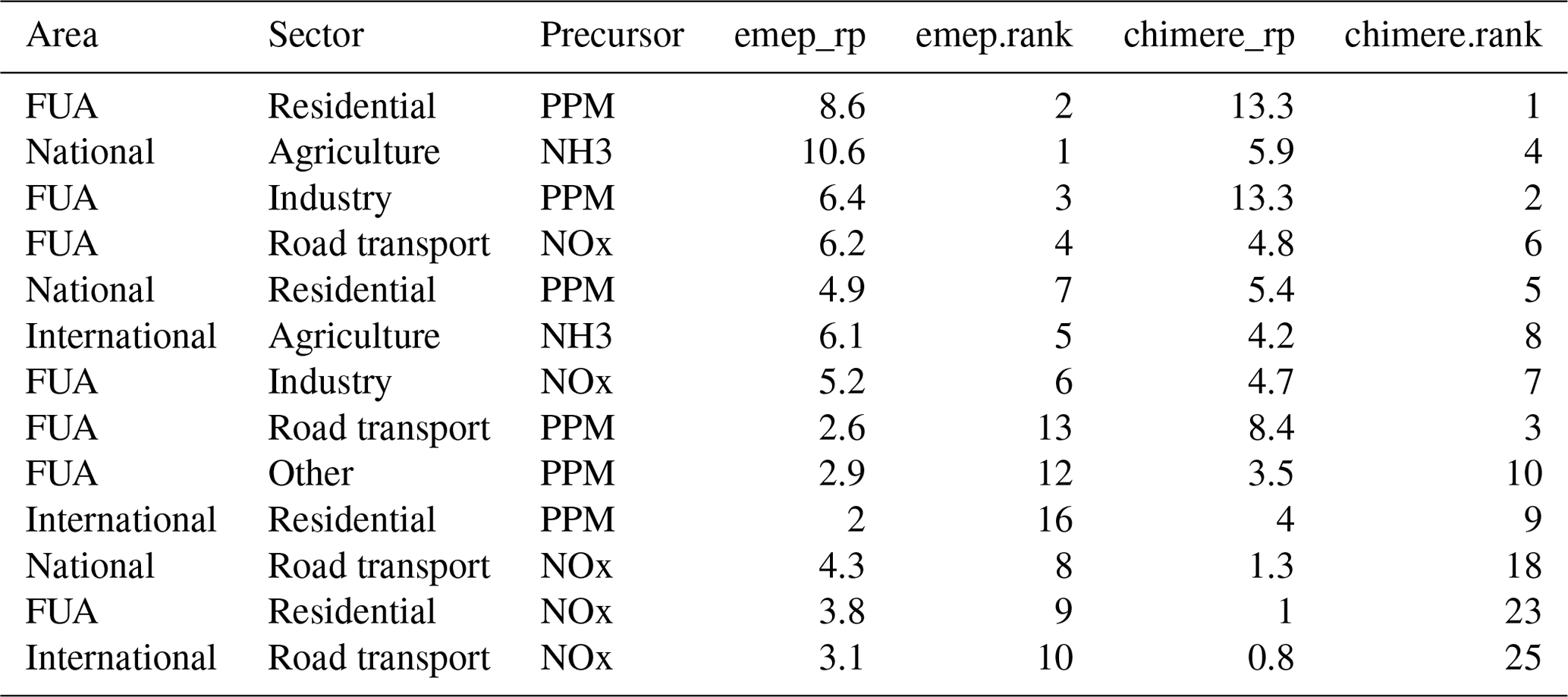
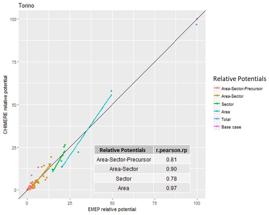
Figure 3 Correlation between S-EMEP and S-CHIMERE relative potentials for different sector–area–precursor source aggregations in Torino (I).

In our last example (Madrid – Table 4 and Fig. 4), differences are extremely important in terms of relative potentials and ranking, leading to an overall correlation of 41 %. All other correlations, with the exception of the spatial ones, are extremely poor. Uncertainties for this city are important, and the choice among policy options is not robust.

Table 4 Top 10 area–sector–precursor relative potentials to PM_2.5 concentrations in Madrid (E).

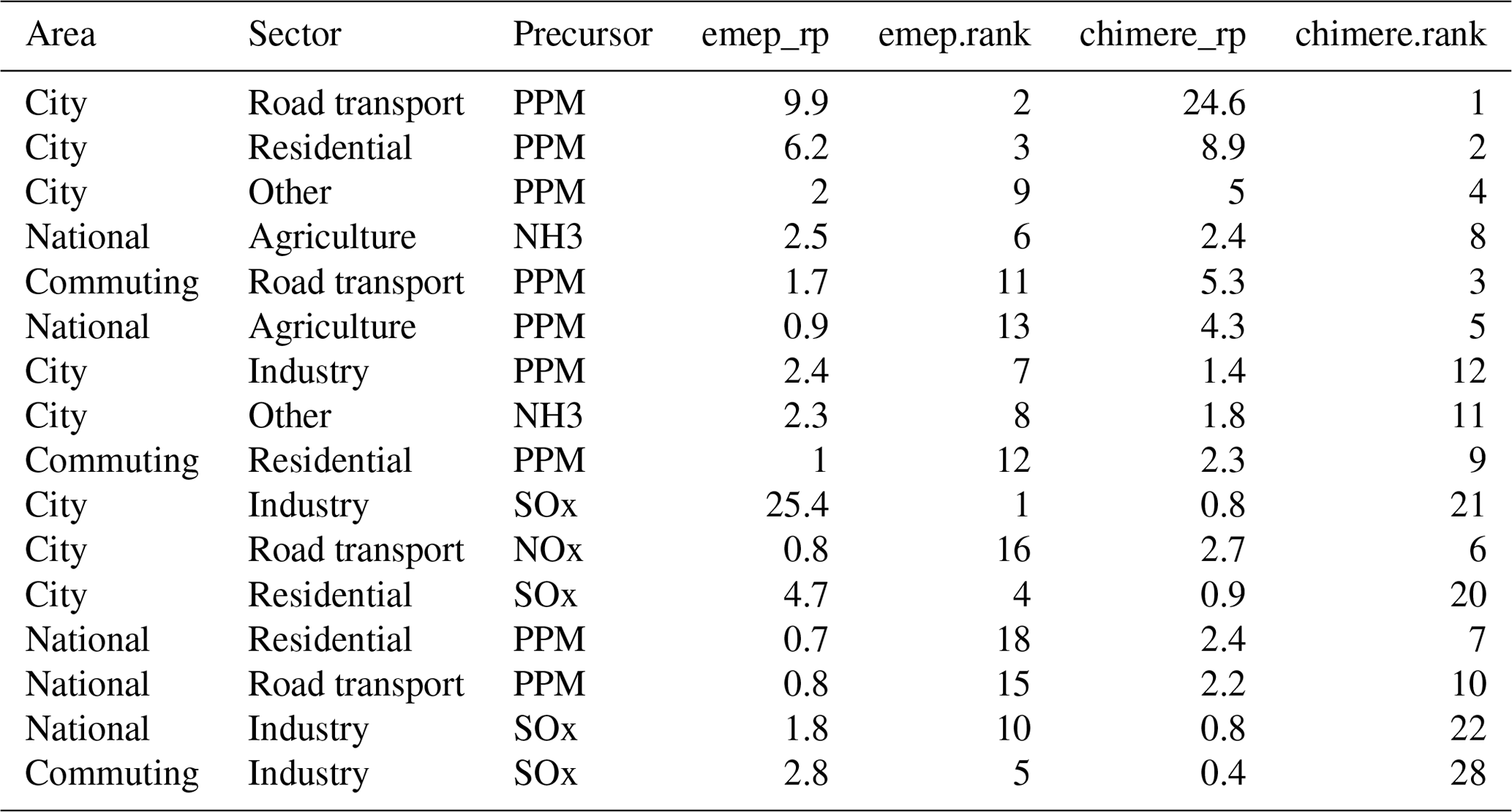
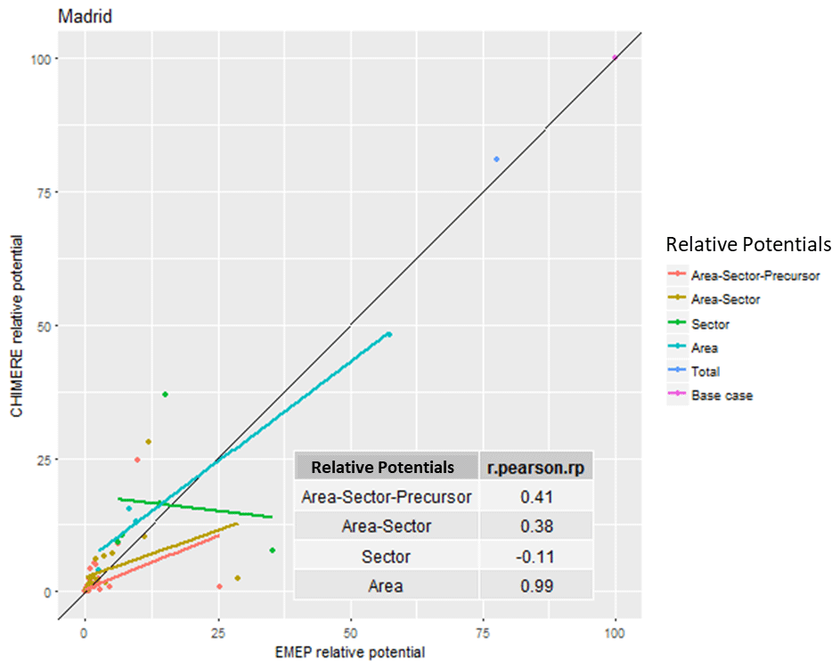
Figure 4 Correlation between S-EMEP and S-CHIMERE relative potentials for different sector–area–precursor source aggregations for Madrid (E).

As seen from the city examples presented above, we can have both strong (Liège) and weak (Madrid) agreement between the two modelling set-ups.

The analysis presented above was done for all 150 cities, and we can here present the results in an aggregated way. We will consider that an overall correlation is very good above 95 %, good between 90 and 95 %, fair between 85 and 90 %, poor between 70 % and 85 %, and very poor below 70 %. This is an arbitrary choice, but it is useful to start grouping and classifying the results. The histogram of the overall correlations for all 150 cities (Fig. 5) shows that the model agreement is good or very good for about half of the cities and satisfactory for another 21 %, leaving 32 % of doubtful or problematic cities.

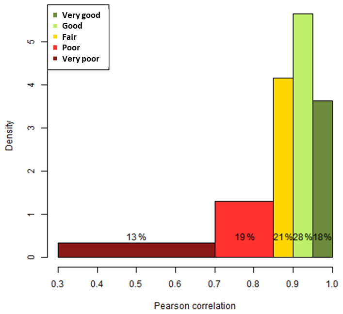
Figure 5 Distribution of the Pearson correlation coefficients between relative potentials, for 150 cities.

The mapping of the overall correlations (Fig. 6) shows that cities with the highest variability are mostly located in Spain, northern Italy and the Baltic countries. For these areas, meteorological factors, emissions and/or the impact of these inputs on concentrations in the air quality models is larger than in other areas. In the Supplement we show that even for the base case, results are quite different for countries like Spain. This might also have an impact on the correlation results shown in this figure.

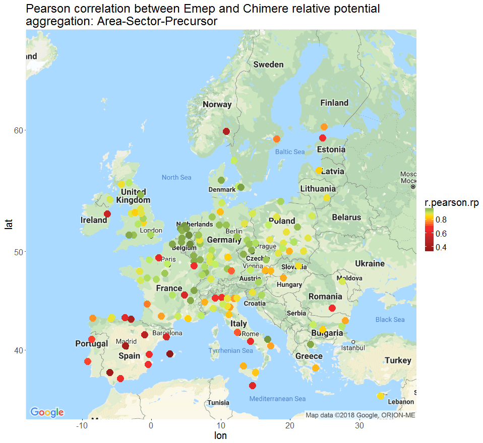
Figure 6 Pearson overall correlation between EMEP and CHIMERE relative potentials.

To the knowledge of the authors, this is one of the first attempts to systematically compare the sources and causes of pollution in European cities using a harmonised approach. The reasons for the differences between cities highlighted above are, however, not easy to identify. This is because the SRRs used in this study are based on different meteorological years (2009 vs. 2014), emissions (2010 vs. 2014) and air quality models (CHIMERE vs. EMEP). Although this analysis provides an overall estimate of the variability between policy responses and does not allow the specific cause for the observed differences to be identified, it indicates where modelling improvements need to be made. Modelling inconsistencies are indeed categorised in terms of geographical area, sectors and precursors, useful information to trigger discussion among modelling groups and direct the investigations towards the most problematic issues.

It is also worth noting that using different input and model set-ups represents the usual practice whenever air quality models are used at the local scale to assess the impact of air quality plans. Indeed, each local and regional authority generally uses its own set of data and applies its own model. Therefore, only a single meteorology, a single emission inventory for a single reference year and a specific model are used to identify the sources of pollution to target. The impact of these choices on source allocation and on the subsequent design of an air quality plan is an issue that is not often tackled.

It is probably unreasonable to think that a local authority can evaluate in a comprehensive way the variability of a particular modelling pathway (too demanding in terms of sensitivity analysis). We, however, believe that this work can be used to develop further guidance to select the proper modelling set-up (choice of meteorological year, emission, model to use) to reduce the uncertainty attached to the results and increase their robustness.

The ultimate goal of this work would be to help decision makers to properly define key sources, so that only “no-regret” policies are selected. As mentioned above, the present approach flags up potential issues and a possible lack of robustness (by quantifying the overall variability), but it cannot provide explanations for the observed differences. The only process to identify the causes of differences is to perform regular inter-comparison exercises where the responses of models to emission changes are systematically tested via sensitivity analysis. While exercises of this type occurred in the past years (Colette et al., 2017; Cuvelier et al., 2007; Pernigotti et al., 2013), it is crucial that these are performed on a regular basis as models and input data continuously evolve.

6 Conclusions

Before applying emission reduction measures to improve air quality, it is important to evaluate the importance of the key sources contributing to pollution in a given area. The main methodology to perform this task is referred to as “source allocation”.

Source allocation can be implemented in various ways. In this paper we use the SHERPA model, a source–receptor relationship mimicking the behaviour of a fully fledged CTM. With SHERPA one can perform hundreds of simulations in a few minutes to test the impact of various geographical, sectoral or precursor-based emission sources on the concentration at a location of interest. The result is a complete source allocation study for a given domain explaining the key sources of pollution at a given location.

In this work, we developed two SHERPA versions, based on two modelling set-ups using different meteorological reference years, emission inventories and air quality models. Even if these settings are quite different and difficult to compare, they represent what happens in the real world when designing air quality plans. Indeed, local authorities in Europe are free to use different reference meteorological years, emissions and models. The comparison of these results therefore provides an estimate of the variability attached to source allocation results for a given area.

The results can also be used to provide further guidance to define the modelling set-up and understand how this choice impacts the selection of priorities when designing air quality plans.

The two SHERPA SRR versions (based on CHIMERE and EMEP) have then been used to perform source allocation on 150 main cities in Europe, and results have been presented in terms of priorities of interventions (i.e. which are the sectors, geographical areas or pollutants that are more relevant for air quality in a given city?).

The results are consistent for some cities, i.e. the modelling set-up produces the same ranking in terms of contributions, whereas for other cities (about 30 %) the two SRRs deliver different results. Even if it is not possible in this work to identify the causes for these differences, as additional sensitivity simulations would be needed for this, this work indicates where modelling improvements need to be made. Modelling inconsistencies are indeed categorised in terms of geographical area, sectors and precursors, useful information to trigger discussion among modelling groups and direct the investigations towards the most problematic issues. Although differences in terms of results were expected (different assumptions deliver different results), it is comforting to see that similar policy decisions would be taken in about 75 % of cities considered in this study.

Thanks to the limited number of required simulations to build SHERPA, future work could envisage the implementation of “constrained settings” to build SRR (i.e. keeping the same air quality model but changing emissions, or keeping the same emissions but changing the model) to be able to discriminate the role of these factors. Also, further model inter-comparison works should be fostered.