Boreal summer intraseasonal oscillation in a superparameterized general circulation model: effects of air–sea coupling and ocean mean state

The effect of air–sea coupling on simulated boreal summer intraseasonal oscillation (BSISO) is examined using atmosphere–ocean-mixed-layer coupled (SPCAM3-KPP, referred to as SPK throughout) and uncoupled configurations of the superparameterized (SP) Community Atmospheric Model, version 3 (SPCAM3, referred to as SPA throughout). The coupled configuration is constrained to either observed ocean mean state or the mean state from the SP coupled configuration with a dynamic ocean (SPCCSM3), to understand the effect of mean-state biases on the BSISO. All configurations overestimate summer mean subtropical rainfall and its intraseasonal variance. All configurations simulate realistic BSISO northward propagation over the Indian Ocean and western Pacific, in common with other SP configurations.

Prescribing the 31 d smoothed sea surface temperature (SST) from the SPK simulation in SPA worsens the overestimated BSISO variance. In both coupled models, the phase relationship between intraseasonal rainfall and SST is well captured. This suggests that air–sea coupling improves the amplitude of simulated BSISO and contributes to the propagation of convection. Constraining SPK to the SPCCSM3 mean state also reduces the overestimated BSISO variability but weakens BSISO propagation. Using the SPCCSM3 mean state also introduces a 1-month delay to the BSISO seasonal cycle compared to SPK with the observed ocean mean state, which matches well with observation. Based on a Taylor diagram, both air–sea coupling and SPCCSM3 mean-state SST biases generally lead to higher simulated BSISO fidelity, largely due to their abilities to suppress the overestimated subtropical BSISO variance.

1 Introduction

The intraseasonal oscillation (ISO) is the most vigorous sub-seasonal signal in the tropics (Zhang, 2005). It interacts with other tropical climate and weather systems, such as the El Niño–Southern Oscillation (ENSO) and tropical cyclones (Kessler et al., 1995; Zhang and Gottschalck, 2002; McPhaden, 2004; Wu et al., 2007), and even the mid-latitude systems (Ding and Wang, 2007; Moon et al., 2013). Compared to the boreal winter ISO (i.e. the Madden and Julian Oscillation, or MJO; Madden and Julian, 1971, 1972), the boreal summer ISO (BSISO) shifts away from the Equator to the Asian summer monsoon (ASM) region (Wang et al., 2006; Lau and Waliser, 2012). Thus, the BSISO is connected strongly to the onset, active, and break phases of the ASM (Yasunari, 1979; Annamalai and Slingo, 2001; Lau and Waliser, 2012). The frequency of extreme events over the ASM region is also highly related to BSISO activity (Ren et al., 2013; Li et al., 2015; Hsu et al., 2016, 2017, 2020; Liu and Hsu, 2019).

Realistic representation of the BSISO in climate models remains a challenge, although some improvements have been achieved in recent decades. The state-of-the-art general circulation models (GCMs) still have difficulty in simulating properly the BSISO spatial pattern (Sperber and Annamalai, 2008; Sperber et al., 2013; Hu et al., 2017) and its northwest–southeast tilted rain band structure (Lin et al., 2006; Sabeerali et al., 2013). In contrast, its northward propagation, which is the most significant feature of the BSISO, is captured by most models. Fidelity for northward propagation improved in the models that contributed to the Coupled Model Intercomparison Project (CMIP) phase 5, relative to the CMIP phase 3 (Sabeerali et al., 2013; Sperber et al., 2013). Most models with reasonable northward propagation of the BSISO also simulate a good eastward propagation along the equatorial Indian Ocean.

The representation of convection is largely responsible for the ability of GCMs to simulate BSISO characteristics (Maloney and Hartmann, 2001; Randall et al., 2007; Jiang et al., 2016). Using the Hadley Centre atmospheric GCM (AGCM), Klingaman and Woolnough (2014) found that increasing the convective entrainment and detrainment rates considerably improved deficient MJO-like variability in the Indian and Pacific oceans. In recent years, studies have shown that “superparameterized” (SP) GCMs have high fidelity in simulating ISO variability (Benedict and Randall, 2009; Jiang et al., 2015; Neena et al., 2017). In SP GCMs, the traditional cumulus parameterization is replaced by a two-dimensional (2-D) cloud-resolving model in each grid column to calculate the cloud and radiation physics tendencies (Khairoutdinov and Randall, 2003; Khairoutdinov et al., 2005). By comparing different versions of the National Center for Atmospheric Research (NCAR) Community Atmospheric Model (CAM), DeMott et al. (2014) showed that the SP CAM (SPA) gave better BSISO characteristics than the CAM with the standard convective parameterization.

Besides the convective parameterization scheme, the effect of air–sea interaction on simulated ISO variability has also received growing attention. By comparing the results of coupled GCMs (CGCMs) with the results of the AGCMs prescribed with observed SSTs, many studies found that the inclusion of air–sea coupling could produce a more realistic intraseasonal variability via improving the representation of the diurnal cycle at the air–sea interface (Waliser et al., 1999; Bernie et al., 2005; Danabasoglu et al., 2006; Misra et al., 2008; Stan, 2018). Besides the air–sea coupling process, the differences between simulated results may also come from ocean mean-state differences between AGCM and CGCM, as incorporating air–sea interaction in CGCMs inevitably introduces atmospheric and ocean mean-state biases. Due to the strong control on low-level moisture and convergence anomalies, such ocean mean-state biases may degrade simulated intraseasonal variability (Hendon, 2000; Inness et al., 2003; Sperber et al., 2005; Bollasina and Ming, 2013). Using the National Centers for Environmental Prediction (NCEP) coupled Climate Forecast System (CFS) model, Seo et al. (2007) showed that BSISO development and propagation were largely improved when the CGCM cold SST bias was removed via flux correction. They suggested that the role of air–sea interaction would be more accurate under an ocean mean state with smaller SST biases. To reduce the mean-state differences between CGCMs and AGCMs, time-varying SSTs from CGCMs should be used to drive AGCMs (Fu and Wang, 2004; Seo et al., 2007; Levine and Turner, 2012; DeMott et al., 2015). However, this quantifies the role of air–sea coupling only under the biased CGCM mean state.

Through flux correction, CGCMs can be constrained to a given climatological ocean state. Such constraint is more effective in CGCMs with simple ocean models, which lack ocean dynamics, as ocean dynamics may interfere with the prescribed flux correction. Simple ocean models also lack coupled modes of variability, such as the ENSO, feedbacks from which can influence the perceived effect of coupling on sub-seasonal variability (Klingaman and DeMott, 2020). The CGCMs with simplified model oceans are a useful tool to investigate the roles of air–sea coupling and mean-state biases in the simulation of BSISO. In this study, we examine the roles of air–sea interaction and mean-state biases in simulated BSISO using a configuration of SPA coupled to a mixed-layer ocean model, constrained to observed ocean mean state and simulated ocean mean state from the SP Community Climate System Model (CCSM), version 3 (SPCCSM3; Stan et al., 2010). The model experiments, validation data, and analysis methods are described in Sect. 2. In Sect. 3, we analyse the influence of air–sea coupling and mean-state biases on the spatial pattern and propagation of simulated BSISO. Results are discussed and summarized in Sects. 4 and 5, respectively.

2 Model, experiments and methods

2.1 Models

SPA (Khairoutdinov et al., 2005) is employed in this study, due to its high fidelity for simulated ISO (Jiang et al., 2015; Neena et al., 2017). It has a horizontal resolution of T42 and a vertical resolution of 30 levels. The embedded 2-D cloud- resolving model has 32 columns with a fine resolution (4 km; Khairoutdinov and Randall, 2003). SPCCSM3 is the coupled configuration, in which SPA is coupled to the 3-D ocean model of the Parallel Ocean Program (POP; Danabasoglu et al., 2006), with active ocean dynamics. SPCCSM3 utilizes the low-resolution version (∼3^∘) of the POP, which has 40 vertical layers with the thickness of top layers being 10 m and exchanges SST and surface fluxes with SPA at 1 d coupling frequency. To understand the roles of air–sea interaction and SST mean-state biases in BSISO simulation, we couple SPA with the Multi-Column K Profile Parameterization (MC-KPP) mixed-layer ocean model, referred to as SPK from now on. In the MC-KPP, there is only vertical mixing (Large et al., 1994), while ocean dynamics, such as horizonal or vertical advection or wind-driven upwelling, are absent. Besides, the air–sea coupled modes of variability (such as the ENSO) and potential feedbacks from these modes to intraseasonal variability are also absent. The MC-KPP consists of many independent 1-D columns, with one column under each AGCM grid for coupling. Therefore, the horizontal resolution of MC-KPP is the same as that of SPA. The MC-KPP has a fine vertical resolution, with 100 points in a 1000 m water column, 70 of which are in the top 300 m, and ∼1 m resolution in the top 20 m. More details on SPK can be found in Klingaman and DeMott (2020).

Since MC-KPP lacks ocean dynamics, SPK must be constrained to a reference ocean climatology, which can be taken from an observation-based dataset, an ocean model simulation, or a CGCM simulation. To represent mean-ocean dynamics and correct for biases in surface fluxes, prescribed vertical profiles of heat and salt corrections are applied at each grid point at each time step. For each SPK simulation analysed here, a 10-year “relaxation” simulation is first performed, with a 15 d relaxation timescale toward the reference seasonal cycles of ocean temperature and salinity. The mean seasonal cycles of the temperature and salinity relaxation tendencies are then computed, smoothed with a 31 d running mean, and imposed as corrections in a “free-running” coupled integration with no relaxation, which displays only small SST biases against the reference climatology (Fig. 1). These free-running simulations are analysed here. More details on the correction method can be found in Hirons et al. (2015) and Klingaman and DeMott (2020).

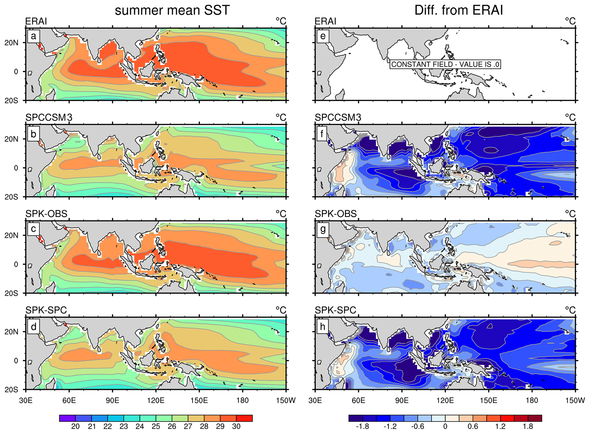
Figure 1 May–October mean SST for (a) ERAI, (b) SPCCSM3, (c) SPK-OBS, and (d) SPK-SPC. Panels (f–h) are calculated differences between (b–d) and (a).

2.2 Experiments and validation data

Two pairs of 50-year-long atmosphere-only (SPA) and coupled (SPK) models were analysed (Table 1). These simulations were also analysed for studying the MJO in Klingaman and DeMott (2020). Next, we explain the set-up of each experiment in detail.

Table 1 List of simulations analysed in this study, including the experiment name, model, ocean climatology condition used by the model to constrain (coupled model) or as forcing (atmospheric-only model), and design purpose.

To study the effect of mean-state biases on simulated BSISO, SPK is constrained to two ocean mean states: (1) the 1980–2009 climatology from the Met Office ocean analysis (Smith and Murphy, 2007) and (2) the climatology from the 20-year SPCCSM3 (“SPC” for short) simulation, which was analysed in Stan et al. (2010) and DeMott et al. (2014). The former is considered as the observed ocean state (Fig. 1c), against which SPC shows large cold SST biases throughout the Indo-Pacific in the boreal summer (Fig. 1f). These two coupled simulations are referred to as “SPK-OBS” and “SPK-SPC”, respectively. Differences between the results of SPK-OBS and those of SPK-SPC can reveal the effect of SPC mean-state SST biases on the simulated BSISO. To investigate the effect of air–sea interaction on simulated BSISO under the observed ocean mean state, the time-varying SSTs from SPK-OBS are prescribed in an SPA simulation (“SPA-KOBS”). The 31 d smoothed SST is used to remove the high-frequency variability of SST and avoid erroneous positive feedbacks between SSTs, surface fluxes, and precipitation (see DeMott et al. (2015) and references therein). Similarly, we prescribe the 31 d smoothed SST from SPK-SPC to SPA to understand the air–sea coupling effect under the SPC mean state (“SPA-KSPC”) through the comparison with SPK-SPC. Table 1 summarizes all four experiments.

The validation data used in this study include (1) daily outgoing longwave radiation (OLR) from the National Oceanic and Atmospheric Administration (NOAA) at a resolution of $\mathrm{2.5}{}^{\circ }\times \mathrm{2.5}{}^{\circ }$ for 1986–2016 (Liebmann and Smith, 1996), (2) daily precipitation from the Global Precipitation Climatology Project (GPCP; Huffman et al., 2001) at a resolution of $\mathrm{1}{}^{\circ }\times \mathrm{1}{}^{\circ }$ for 1997–2016, and (3) daily variables from the European Centre for Medium-range Weather Forecasts (ECMWF) Interim (ERAI) reanalysis dataset at a resolution of $\mathrm{1.5}{}^{\circ }\times \mathrm{1.5}{}^{\circ }$ (Dee et al., 2011). The variables from the ERAI include 850 hPa wind, SST, surface variables related to latent heat and sensible heat (LH and SH) fluxes, and 3-D variables associated with moist static energy (MSE; Maloney, 2009). Note that ERAI SST was the boundary condition prescribed for the ERAI. We analyse the period of 1986–2016 of ERAI data for compatibility with Gao et al. (2019).

2.3 Methods

The BSISO convective intensity is represented by 20–100 d filtered variability of boreal summer (May–October) precipitation, OLR, or MSE, depending on the process-oriented diagnostic applied. To reveal the overall propagation features of BSISO convection, lead-lag regression analysis is performed on area-averaged, filtered precipitation or OLR. Here, we use precipitation. Since the Indian and Pacific basins exhibit different basic states (Lau and Waliser, 2012), we compute propagation over one region in each basin: the eastern Indian Ocean (0–10^∘ N, 80–90^∘ E) and western Pacific (0–10^∘ N, 130–140^∘ E).

DeMott et al. (2016) and Gao et al. (2019) provided a useful diagnostic method to quantitatively assess the contribution of intraseasonal SST variability to the MSE budget of ISO in the boreal winter and boreal summer, respectively. The temporal and spatial evolution of column-integrated MSE (〈m〉) is highly consistent with that of anomalous precipitation; and positive values of the time change of 〈m〉 ($\partial \langle m\rangle /\partial t$) leads 90^∘ ahead of the convection. Thus, the physical processes that modulate 〈m〉 and $\partial \langle m\rangle /\partial t$ can be considered as the mechanisms responsible for the maintenance and propagation of convections, respectively. We employ the same approach to understand oceanic feedbacks to the simulated BSISO and compare these feedbacks to those in reanalysis data. Intraseasonal SST can affect atmospheric convection through modifying LH and SH fluxes and hence MSE, via the near-surface gradients in specific humidity and temperature. Based on decomposition of surface bulk formulae (Weare et al., 1981), SST modulation of surface fluxes is represented as the difference between fluxes calculated using the full and 61 d smoothed SST. These SST-modulated fluxes are then projected onto 〈m〉 and $\partial \langle m\rangle /\partial t$ to reveal the oceanic feedbacks to the maintenance and propagation of BSISO convection, respectively. More details can be found in DeMott et al. (2016) and Gao et al. (2019).

Figure 2 May–October mean precipitation (shading) and 850 hPa wind (vector; with amplitude > 3.5 m s⁻¹) for (a) GPCP precipitation and ERAI 850 hPa wind, (b) SPK-OBS, and (c) SPK-SPC. Panels (e, f) are calculated differences between (b, c) and (a).

We employ the BSISO indices of Lee et al. (2013) to investigate the simulated convective features in each BSISO phase. First, daily anomalies are computed as the departure from the climatological annual cycle and a 120 d running mean. A multi-variate empirical orthogonal function (MV-EOF) is then performed on the combination of OLR and 850 hPa zonal wind (u₈₅₀) anomalies, each normalized by their respective area-mean standard deviation over the ASM region (10^∘ S–40^∘ N, 40–160^∘ E) during the boreal summer. The first two leading principal components (PC1 and PC2) define the BSISO indices, which separate the BSISO life cycle into eight phases. For model results, normalized OLR and u₈₅₀ anomalies are projected onto the observed EOF modes to obtain the model PCs. This approach helps to fairly assess how well the model experiments simulate the observed BSISO because the projected results (model PCs) can be directly compared to observations (Sperber et al., 2008, 2013; DeMott et al., 2019). Model-simulated BSISO phase composites are constructed based on these PCs. Consistent with Lee et al. (2013), only strong BSISO events ($\sqrt{\mathrm{PC}{\mathrm{1}}^{\mathrm{2}}+\mathrm{PC}{\mathrm{2}}^{\mathrm{2}}}>\mathrm{1.5}$) are selected for phase composites.

3 Results

3.1 Mean state and intraseasonal variability

Previous studies indicated that ISO variability is closely related to the climatological state of convection (Wheeler and Kiladis, 1999; Sperber et al., 2000; Waliser et al., 2003). Thus, we first examine the summer mean precipitation and 850 hPa wind (Fig. 2). In GPCP, substantial rainfall appears over the ASM region (Fig. 2a). In common with the SPA simulation (DeMott et al., 2011), SPK-OBS overestimates subtropical rainfall (10–20^∘ N), particularly in the western North Pacific (Fig. 2b and e), but underestimates rainfall over the southern Indian Ocean, Maritime Continent and India north of 20^∘ N. These precipitation biases are associated with low-level wind biases. Simulated mean westerlies extend into the western North Pacific, increasing convergence across the band of subtropical enhanced precipitation. In SPK-SPC (Fig. 2c), which is constrained to the cold climatological SPC SST (Fig. 1d), rainfall is reduced compared to that in SPK-OBS: wet biases are reduced while dry biases become more severe over the Indian Ocean and western North Pacific (Fig. 2e and f). The SPC mean-state SST bias tends to suppress the mean precipitation. Mean precipitation fields in SPA-KOBS and that in SPK-OBS (SPA-KSPC and SPK-SPC) are nearly the same (not shown).

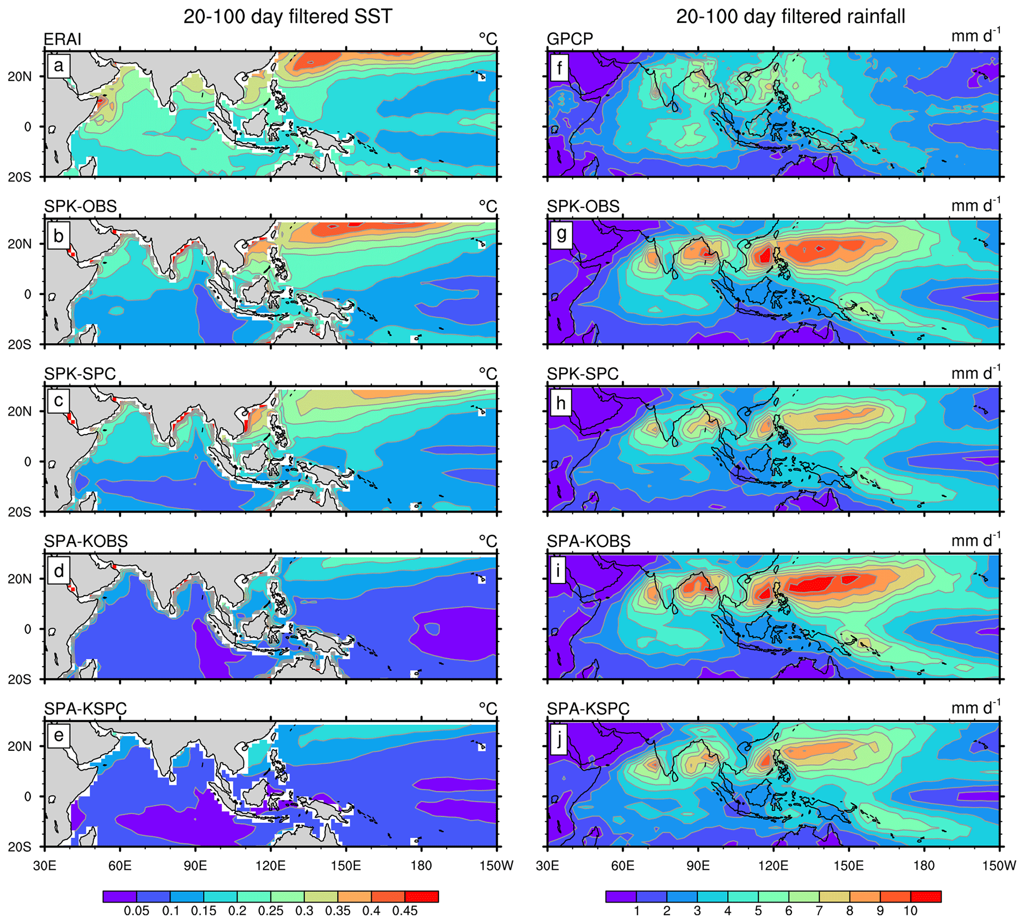
Figure 3 May–October standard deviations of 20–100 d filtered (a–e) SST and (f–j) precipitation for (a, f) ERAI SST and GPCP precipitation, (b, g) SPK-OBS, (c, h) SPK-SPC, (d, i) SPA-KOBS, and (e, j) SPA-KSPC.

Figure 3 illustrates the standard deviations of intraseasonal SST and precipitation variability. SST variability is underestimated over the Indian Ocean and equatorial Pacific in all simulations. In the off-equatorial Pacific, we see more intraseasonal SST variability in SPK-OBS but less SST variability in SPK-SPC (Fig. 3b and c), which may be related to the less SST variability in SPC as a consequence of a coarse horizontal resolution of POP. Prescribing the 31 d smoothed SST from SPK-OBS (SPK-SPC) to SPA-KOBS (SPA-KSPC) strongly reduces intraseasonal SST, as expected (Fig. 3d and e). The right-column panels in Fig. 3 show the intraseasonal rainfall from each dataset (Fig. 3f–j). Compared to GPCP (Fig. 3f), all simulations significantly overestimate subtropical intraseasonal precipitation variability (10–20^∘ N), where mean rainfall is also overestimated (Fig. 2). This reinforces that model BSISO biases are largely associated with incorrect representation of mean rainfall (Sperber and Annamalai, 2008; Sabeerali et al., 2013; Hu et al., 2017). The overestimate of intraseasonal rainfall in SPK-SPC (Fig. 3h) is smaller than that in SPK-OBS (Fig. 3g), consistent with the lower mean rainfall in SPK-SPC. SPA-KOBS (Fig. 3i) and SPA-KSPC (Fig. 3j) show increases in intraseasonal rainfall relative to SPK-OBS and SPK-SPC, respectively. This indicates that both cold SST biases and air–sea coupling exert negative feedbacks on BSISO convection and improve the simulated BSISO amplitude.

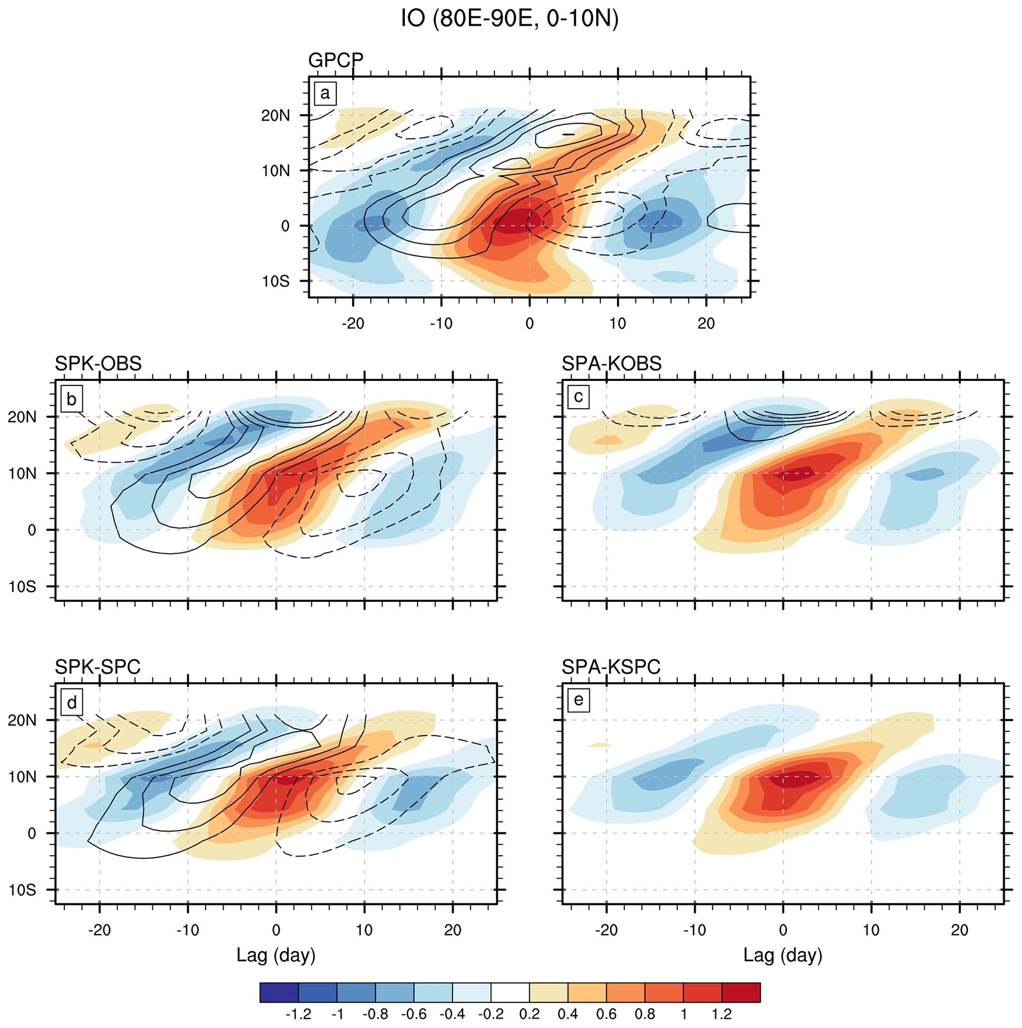
Figure 4 Lagged regression coefficients of 80–90^∘ E averaged intraseasonal precipitation (shading; mm d⁻¹ (mm d⁻¹)⁻¹) and SST (contour; ^∘C (mm d⁻¹)⁻¹) onto (0–10^∘ N, 80–90^∘ E) averaged intraseasonal precipitation for (a) GPCP precipitation and ERAI SST, (b) SPK-OBS, (c) SPA-KOBS, (d) SPK-SPC, and (e) SPA-KSPC. Contour interval is 0.001 ^∘C (mm d⁻¹)⁻¹, and zero contour is omitted.

3.2 Northward propagation of BSISO

Lag regression analysis is employed to understand the simulated BSISO propagation in each experiment. Over the Indian Ocean, area-averaged intraseasonal precipitation and SST (over 80–90^∘ E) are regressed onto area-averaged intraseasonal precipitation (over 0–10^∘ N, 80–90^∘ E) time series (Fig. 4). In observation, the convective anomaly originates south of the Equator and propagates southward to 10–15^∘ S and northward into the Bay of Bengal (Fig. 4a). All simulations capture the northward propagation, confirming the high fidelity of SPA in simulating BSISO northward propagation (DeMott et al., 2014; Neena et al., 2017). However, the simulations fail to capture the southward propagation branch. Other significant biases can be seen in the locations of maximum convections of BSISO. The simulated convective centre shifts northward (10^∘ N) relative to observation (5^∘ N). A weaker propagating signal is observed under the SPC mean state than under the observed mean state for both SPK and SPA, especially over the subtropical regions from Lag 0 to Lag 20 (Fig. 4b–e). This is consistent with weaker BSISO variability under the SPC mean state (Fig. 3g–j), suggesting that cold tropical mean SST biases are unfavourable for BSISO variability and northward propagation. In SPA, the amplitude of convective maxima increases relative to that in SPK, but with weaker propagation (Fig. 4b–e). Air–sea coupling plays a similar role in BSISO convection under both observed and cold mean states: it damps BSISO amplitude but supports northward propagation over the eastern Indian Ocean.

The BSISO northward propagation over the western Pacific is shown in Fig. 5. The observed convection also originates south of the Equator but propagates only north, into the western North Pacific (Fig. 5a). These characteristics are properly simulated by all experiments (Fig. 5b–e). As in the Indian Ocean, due to the large overestimate of subtropical BSISO variability, the strongest simulated convection moves north compared to observation. It is notable that considerable suppressed off-equatorial convection leads the strongest convection by ∼1 week, which degrades model performance. Over the western Pacific, mean-state biases also reduce the northward propagating signal in SPK-SPC (SPA-KSPC) relative to that in SPK-OBS (SPA-KOBS). Air–sea interaction seems to play only a small role in the BSISO northward propagation over the western Pacific, as there is no substantial difference between SPK and SPA under either ocean mean state (Fig. 5b–e).

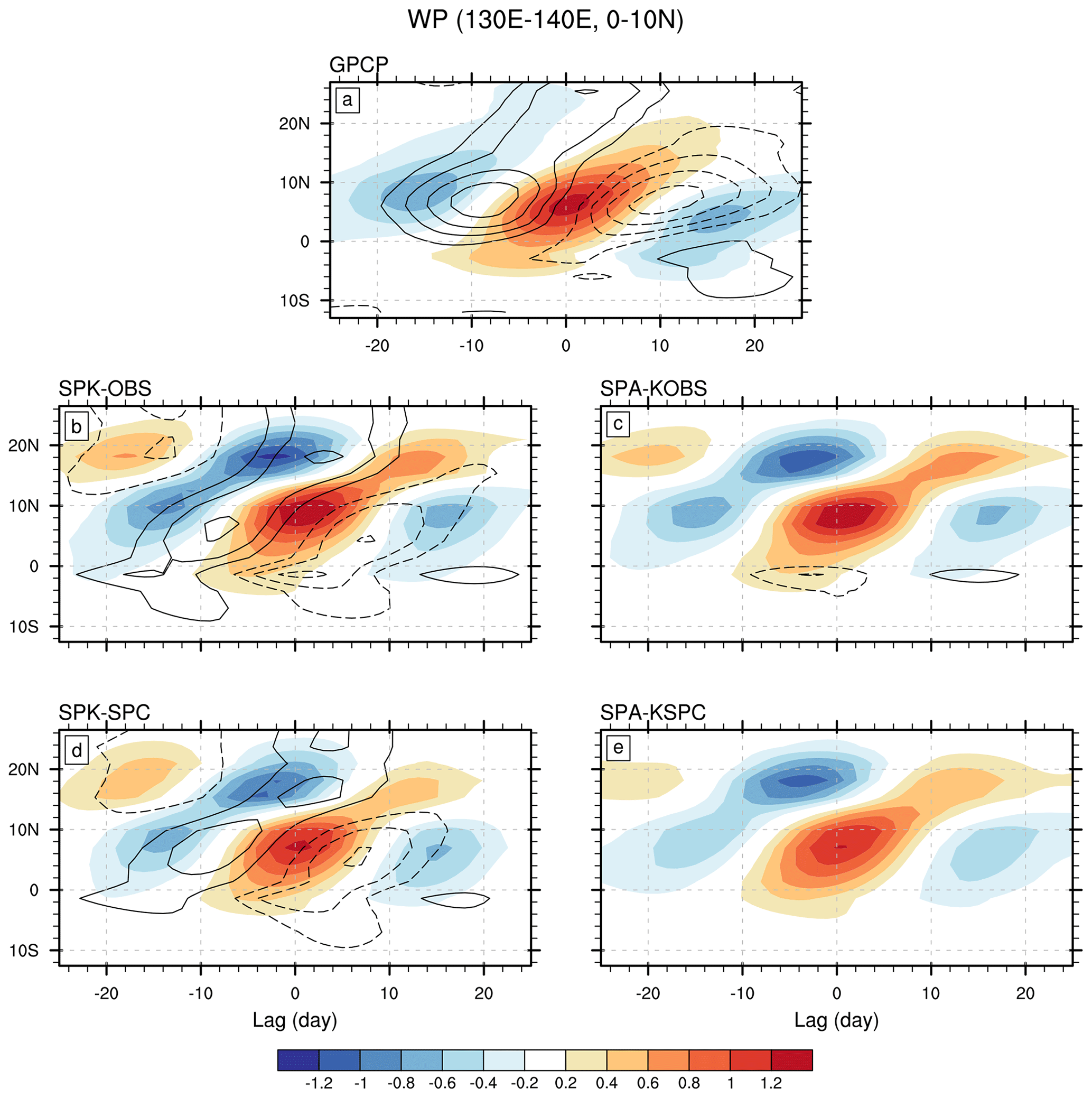
Figure 5 Same as Fig. 4, except for 130–140^∘ E averaged intraseasonal precipitation and SST regressed onto (0–10^∘ N, 130–140^∘ E) averaged intraseasonal precipitation.

3.3 Quantitative contribution of SST fluctuation to BSISO

The temporal and spatial evolutions of BSISO and SST variability over the Indian Ocean and western Pacific are shown in Figs. 6 and 7, respectively. Over the Indian Ocean, the warm SSTs in observation always lead enhanced convection, with maxima north-northeast of the convective centre (Fig. 6a, f, and k). The SST–rainfall phase relationship is properly represented in SPK but misrepresented in SPA. However, SPK shows a shorter delay between off-equatorial suppressed convection and warm SST relative to observation, which can be more clearly revealed in Fig. 4. This suggests the ocean responds more quickly to BSISO convection in SPK than in observation, which might be caused by the lack of ocean dynamics in MC-KPP. Alternatively, the high coupling frequency (15 min) and fine ocean vertical resolution (∼1 m) in SPK may make the mixed-layer depth too sensitive to atmospheric convection. The SST anomalies in SPA are small due to the 31 d smoothing applied (Fig. 6d, e, i, j, n, and o). The size of the convective regions in all model simulations is smaller than that in observations, which may imply a deficient BSISO propagation. Compared to SPK-OBS, the convective region reduces when either the SPC mean state is used (SPK-SPC) or air–sea coupling is removed (SPA-KOBS and SPA-KSPC). To some degree, it reflects the negative (positive) role of mean-state biases (air–sea interaction) in supporting the propagating BSISO signal, in agreement with Fig. 4.

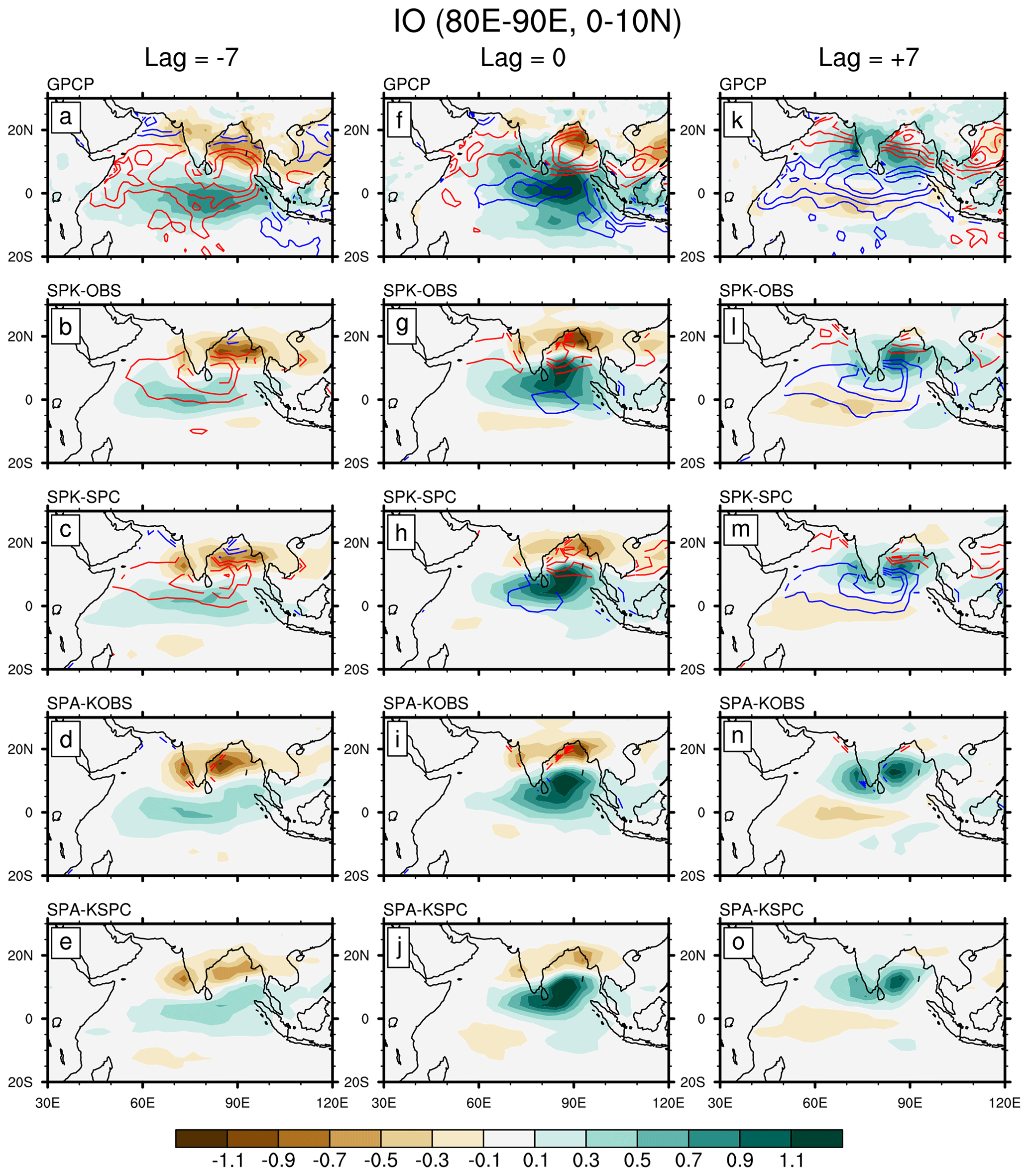
Figure 6 Regression coefficients of intraseasonal precipitation (shading; mm d⁻¹ (mm d⁻¹)⁻¹) and SST (contour; ^∘C (mm d⁻¹)⁻¹) onto (0–10^∘ N, 80–90^∘ E) averaged intraseasonal precipitation over the Indian Ocean at lags of (a–e) −7, (f–j) 0, and (k–o) +7 d, for (a, f, k) GPCP precipitation and ERAI SST, (b, g, l) SPK-OBS, (c, h, m) SPK-SPC, (d, i, n) SPA-KOBS, and (e, j, o) SPA-KSPC. The contour interval is 0.01 ^∘C (mm d⁻¹)⁻¹; positive (negative) values are represented by red (blue) lines.

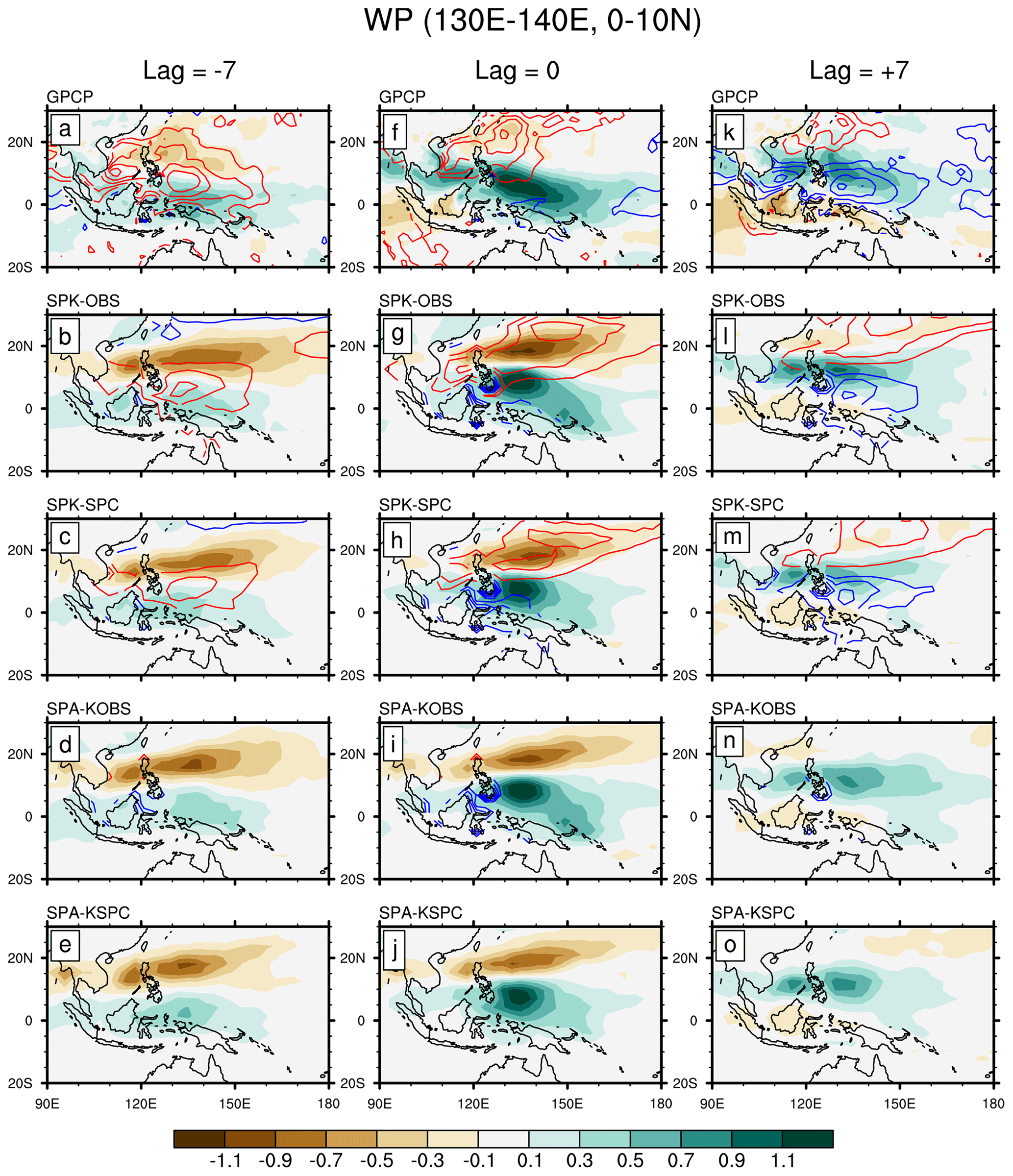
Figure 7 Same as Fig. 6, except for variables regressed onto (0–10^∘ N, 130–140^∘ E) averaged intraseasonal precipitation over the western Pacific.

Over the western Pacific, SPK reproduces the observed phase relationship between the convection and SST anomalies: a near-quadrature relationship over the equatorial regions (Fig. 7a–c), but a shift of warm SST anomalies toward the suppressed convective regions in the off-equatorial regions (Fig. 7f–h and k–m). This phase relationship can also be clearly revealed in the Hovmöller diagram (Fig. 5). However, SPK produces substantial suppressed convection north of the active convection over the western North Pacific, consistent with Fig. 5. Besides, a simulated warm SST appears north of the convective centre, while the ERAI SST maximum is always located northwest of the convective centre. This implies that the simulated SST may be favourable for the northward but unfavourable for the westward propagation of the simulated BSISO convection over the western Pacific. Imposing the SPC mean state weakens the simulated convection. In SPA, the intraseasonal SST is very small by design.

As revealed by Gao et al. (2019), intraseasonal SST can affect the BSISO by modulating surface LH and SH fluxes. The temporal and spatial distributions of SST-modulated fluxes are highly coherent with those of SST anomalies themselves. Therefore, the evolutions of SST anomalies shown in Figs. 6 and 7 can also roughly reveal the evolutions of SST-modulated surface fluxes. By regressing the SST-modulated flux anomalies onto the BSISO 〈m〉 and $\partial \langle m\rangle /\partial t$, Fig. 8 illustrates the “SST effect” on the maintenance and propagation of convection. In the ERAI, intraseasonal SST supports 〈m〉 in the central Indian Ocean and Bay of Bengal but destroys 〈m〉 in the western North Pacific (Fig. 8a). The inter-basin differences are linked to the differences in the SST–convection phase relationship (Gao et al., 2019). However, simulated SST anomalies in SPK largely damp the convection over the Bay of Bengal and western North Pacific (Fig. 8b and c), because of the quicker response of the SPK ocean to BSISO convection, combined with the erroneously strong suppressed convection just before the active phase. The negative SST effect on 〈m〉 agrees with the stronger subtropical BSISO variability in SPA than in SPK. For the BSISO propagation, the simulated SST anomalies play positive roles in $\partial \langle m\rangle /\partial t$ under both ocean mean states (Fig. 8g and h), but with a smaller contribution (8 %–12 %) than that in the ERAI (12 %–20 %). A weak SST effect on the BSISO can still be found in SPA (Fig. 8d, e, i, and j), as these simulations retain some intraseasonal SST variability (Fig. 3). In summary, SST variability enhances the simulated amplitude of BSISO variability by suppressing the excessive subtropical convection and contributes to the propagation of convection over the entire BSISO region.

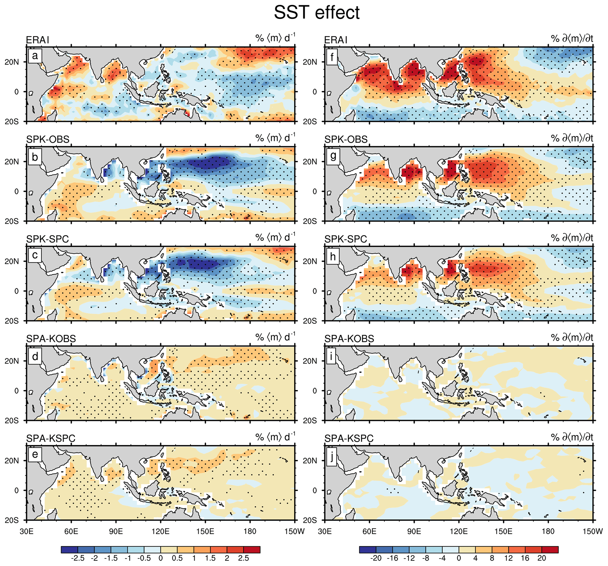
Figure 8 SST effect on (a–e) 〈m〉 and (f–j) $\partial \langle m\rangle /\partial t$ through the modification of surface turbulent fluxes for (a, f) ERAI, (b, g) SPK-OBS, (c, h) SPK-SPC, (d, i) SPA-KOBS, and (e, j) SPA-KSPC. Stippling indicates regression coefficient is significant at the 95 % confidence level.

3.4 BSISO indices

Propagating BSISO characteristics can also be examined using the BSISO indices. Figure 9 shows the annual cycle of variance of each of the first four PCs from observation and model simulations. Since EOF analysis is only applied to May–October data, the PC time series for November–April are obtained by projecting OLR and u₈₅₀ anomalies onto the same EOF patterns.

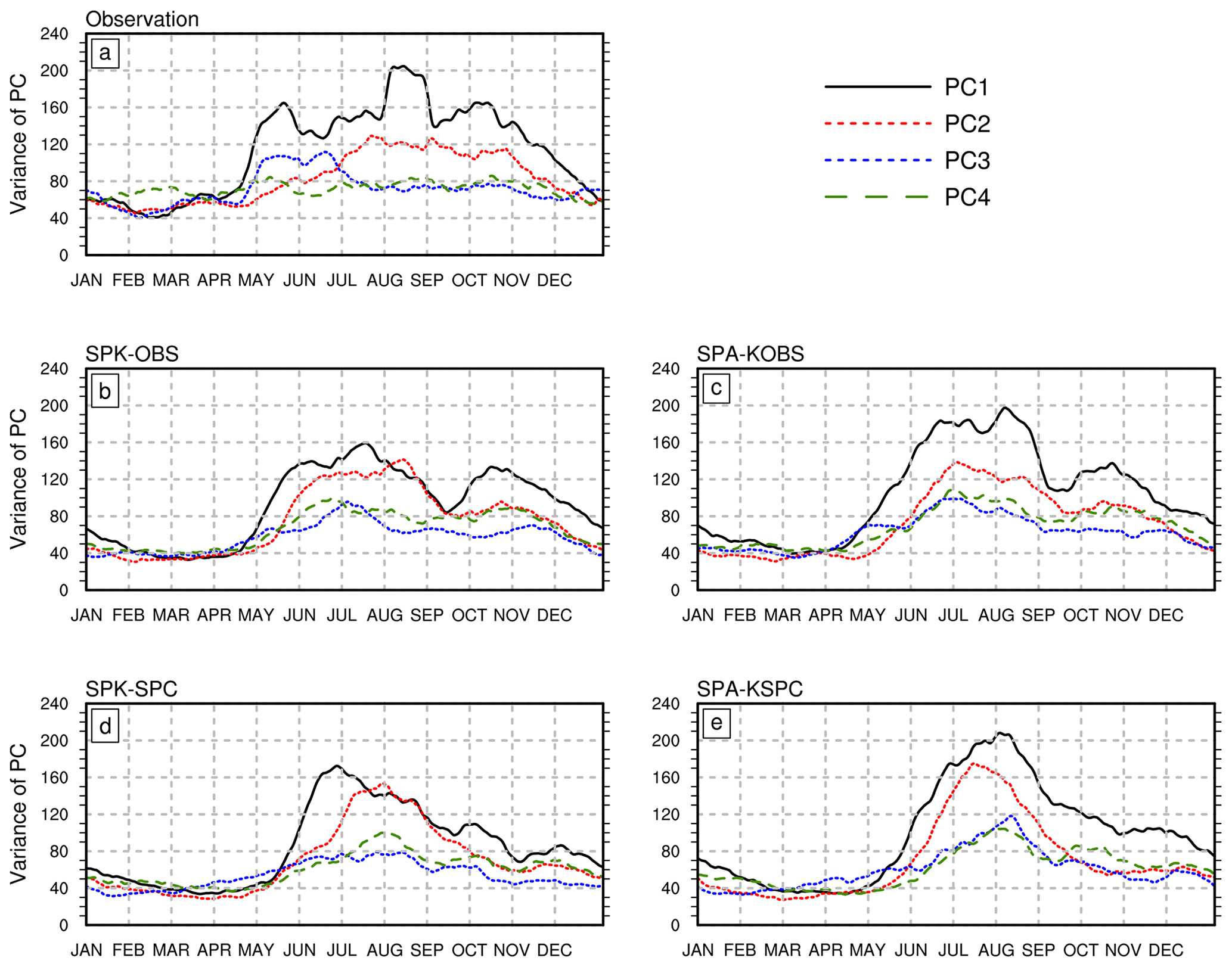
Figure 9 Seasonal cycle of variance of the four leading PCs for (a) NOAA OLR and ERAI u₈₅₀, (b) SPK-OBS, (c) SPA-KOBS, (d) SPK-SPC, and (e) SPA-KSPC. A 30 d running mean is applied to the seasonal cycle of each variable.

In observation, PC1 has the largest variance throughout the boreal summer (Fig. 9a). It increases sharply from late April, maximizes in August, and is followed by PC2 with about a half-month delay. In contrast to PC1 and PC2, PC3 exhibits most of its variance in early summer (May–June). PC4 also has a broad peak, but its amplitude is much smaller than those of the other PCs. SPK-OBS produces a similar seasonal cycle of PC1 as observation, except for deficient variance in August–September, which largely reduces the amplitude difference between the first two PCs (Fig. 9b). Simulated PC1 in SPK-OBS also increases abruptly from late April, with a half-month delay between PC1 and PC2, which matches the observation well. However, PC1 in SPK-SPC begins to increase in late May (Fig. 9d), about 1 month later than the observation and SPK-OBS. The variance of the first two PCs in SPK-SPC has a much narrower peak and tails off from early July, without a second peak in October. This suggests that cold SST bias leads to a late onset of BSISO activity, and also strongly degrades the annual cycle of BSISO activity. In both SPK simulations, the amplitude of PC3 is smaller than that of PC4, indicating that the order of those simulated PCs is reversed. All model simulations show a similarly poor ability to simulate PC3 and PC4. Therefore, hereafter we only focus on PC1 and PC2. Removing air–sea coupling in SPA significantly increases the strength of PC1 relative to that in SPK (Fig. 9b–e). This suggests that the role of air–sea coupling in suppressing BSISO variability is mainly expressed through damping variability in PC1.

Based on the PC1 and PC2 time series, the BSISO life cycle is separated into eight phases, which represents the canonical northward-propagating BSISO (Annamalai and Sperber, 2005; Wang et al., 2005). Figure 10 shows the phase composites of anomalous precipitation and 850 hPa wind from the observation and SPK-OBS. SPK-OBS displays a similar evolution of the structure of convection and circulation as the observation, but they have significant amplitude differences. The simulated precipitation variability is underestimated over the equatorial Indian Ocean, while a substantial overestimate appears over the off-equatorial regions. The simulated circulation matches well with the simulated convection: easterlies (westerlies) occur to the north (south) of the ascent; cyclonic (anticyclonic) circulations coincide with the active (suppressed) off-equatorial convection. However, the northwest–southeast tilted rainfall band in SPK-OBS is more zonal than that in GPCP (Fig. 10e and m), largely due to the poor representation of BSISO variability over the western Pacific. In observation, most strong BSISO events occur in phases 2, 5, 7, and 8. In contrast, in SPK-OBS, a stronger preference for simulated strong BSISO events appear in off-equatorial regions (phases 3, 4, 7, and 8) rather than in near-equatorial regions (phases 1, 2, 5, and 6). It implies that the BSISO variability is largely determined by the propagating BSISO signal (Sperber et al., 2013; Neena et al., 2017).

Figure 10 Composites of anomalous precipitation (shading; mm d⁻¹) and 850 hPa wind (vector; with amplitude > 1 m s⁻¹) in the BSISO life cycle from phase 1 to phase 8 for (a–h) GPCP precipitation and ERAI 850 hPa wind and (i–p) SPK-OBS. The number of days for the phase composite is shown at the right corner above each panel. Only strong BSISO events (amplitude ≥ 1.5) are selected.

We further compute the frequency of strong BSISO events in each phase from each dataset (Fig. 11). Overall, there are fewer strong BSISO events in the simulations (22.5 %–27.5 %) than in observation (∼33 %), although the amplitude of simulated precipitation associated with these events is much larger. The frequency of stronger BSISO events becomes further reduced under the SPC ocean mean state than that under the observed ocean mean state. Consistent with Fig. 10, phases 2, 5, 7, and 8 show the highest frequencies in observation, while in SPK-OBS and SPK-SPC, most strong simulated BSISO events occur in phases 3, 4, 7, and 8. Removing air–sea coupling in SPA further increases the frequency of strong BSISO events in the off-equatorial regions, associated with the greater intraseasonal convective variability in SPA relative to that in SPK.

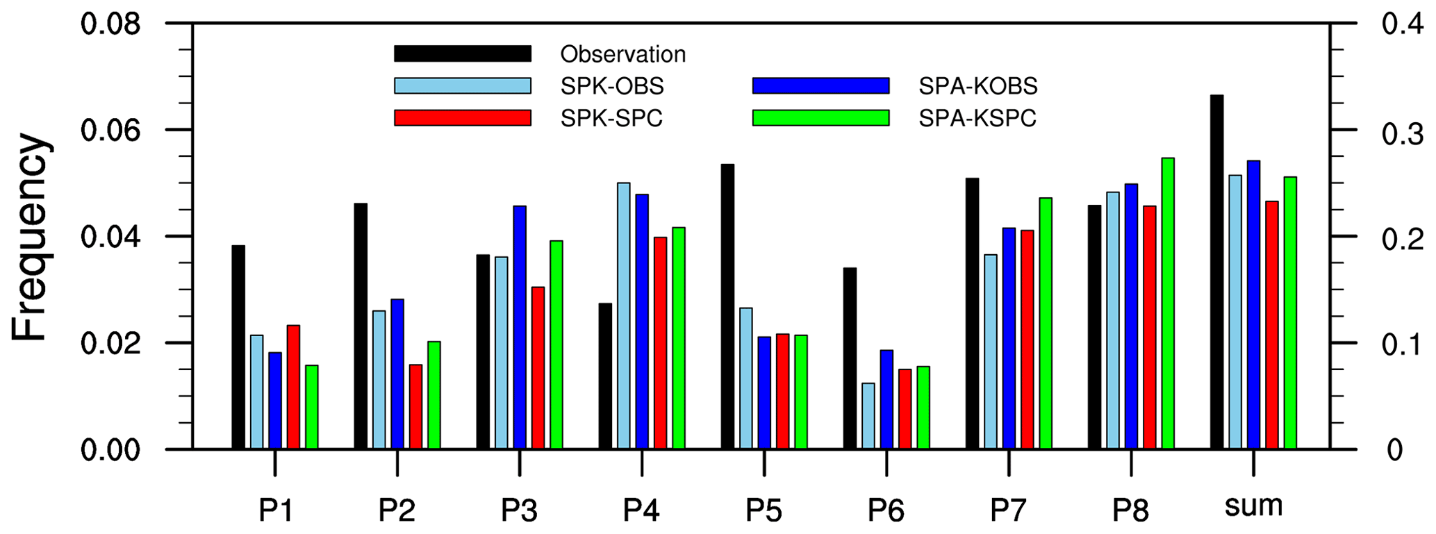
Figure 11 The frequency of strong BSISO activity (amplitude ≥ 1.5) in each phase (P1–P8; the left y axis) and their sum (the right y axis) for NOAA OLR and ERAI u₈₅₀ (black), SPK-OBS (light blue), SPA-KOBS (dark blue), SPK-SPC (red), and SPA-KSPC (green).

To quantitatively evaluate the performance of each simulation, we construct Taylor diagrams over the Indian Ocean (10^∘ S–20^∘ N, 50–100^∘ E) and western Pacific (0–30^∘ N, 110–160^∘ E), respectively (Fig. 12). These diagrams provide pattern correlation coefficients and root-mean-square errors of simulated intraseasonal precipitation against GPCP intraseasonal precipitation in each BSISO phase. Over the Indian Ocean, the fidelity of each simulation varies from phase to phase (Fig. 12a). Generally, higher pattern correlations appear in equatorial phases (phases 1, 2, 5, and 6) than in off-equatorial phases (phases 3, 4, 7, and 8). Under the observed ocean mean state, air–sea coupling improves the simulation fidelity in most phases, while the SPC ocean mean state and coupling under the SPC ocean mean state have little consistent effect on the simulated BSISO fidelity.

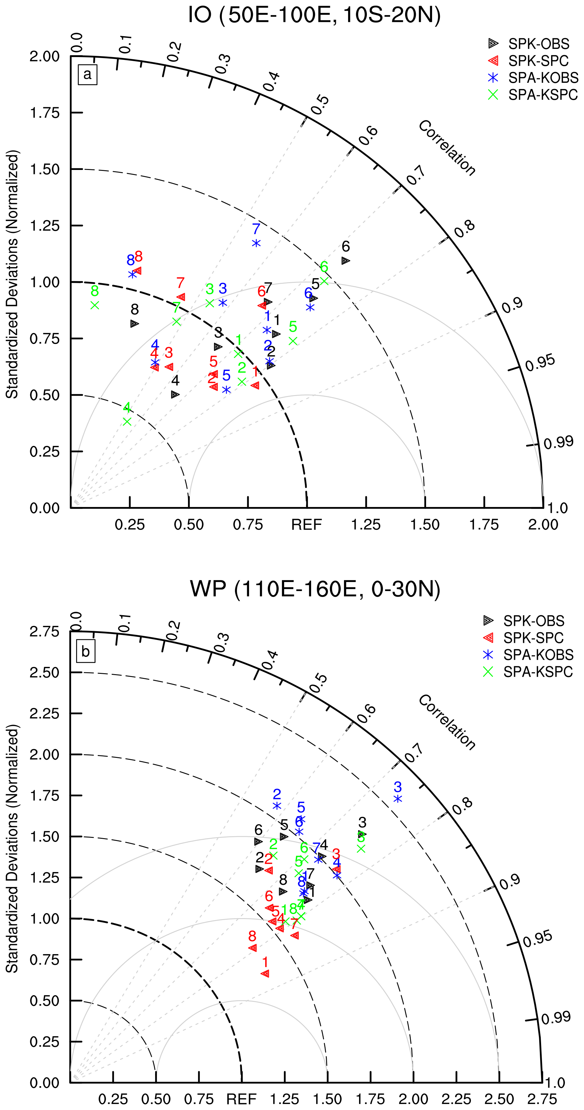
Figure 12 Taylor diagrams for anomalous precipitation in each BSISO phase averaged over (a) the Indian Ocean (IO; 10^∘ S–20^∘ N, 50–100^∘ E) and (b)  western Pacific (WP; 0–30^∘ N, 110–160^∘ E). The number above each symbol refers to the BSISO phase.

In almost all simulations, higher pattern correlations are found over the western Pacific (0.6–0.9) than over the Indian Ocean (0.5–0.8), but with much larger overestimates of amplitude (Fig. 12b). The overall simulation performance over the western Pacific is ranked as follows: SPK-SPC, SPA-KSPC, SPK-OBS, and SPA-KOBS. Simulations with the SPC ocean mean state perform better than those with the observed ocean mean state, in terms of both amplitude and distribution. Since the excessive subtropical rainfall variability is the biggest error in SPA, the underlying cold SSTs largely weaken the convection, which helps reduce the amplitude biases and improve the pattern correlation with observation. Air–sea coupling improves model performance under both ocean mean states, particularly in terms of suppressing the overestimated BSISO variability over the western North Pacific.

4 Discussion

Despite the correct SST–rainfall phase relationship in SPK simulations, a shorter delay between suppressed convection and warm SST occurs compared to the observation. This may be associated with the configuration of the MC-KPP ocean (lack of full ocean dynamics, high coupling frequency, and fine vertical resolution). As a consequence of the shorter delay, it is easy to surmise the negative effect of air–sea coupling on the amplitude of convection, while its effect on the propagation is not obvious. Overall, intraseasonal SST anomalies in SPK largely damp intraseasonal subtropical convection variability and make a smaller contribution (8 %–12 %) to $\partial \langle m\rangle /\partial t$ than those in the ERAI (12 %–20 %). Comparing Figs. 4 and 5, we can see propagation is slightly enhanced in SPK relative to SPA over the Indian Ocean; however, coupling makes nearly no difference to the propagating signal over the western Pacific. This may be related to the larger underestimate of the contribution of intraseasonal SST to $\partial \langle m\rangle /\partial t$ over the western Pacific than over the Bay of Bengal (Fig. 8). More importantly, it implies that atmospheric internal processes are essential to the propagation of convection, since SPA simulates BSISO propagation well even without coupling or sub-seasonal SST variability.

Stan et al. (2010) and Neena et al. (2017) reported that SPC showed better ISO simulation skill than SPA with prescribed observed SST. In our experiments, the BSISO variability is similar in SPK-OBS and SPA-KOBS and in SPK-SPC and SPA-KSPC, which suggests a limited role for air–sea coupling in the simulated BSISO. Comparing SPK-OBS and SPK-SPC strongly suggests that the ocean mean-state biases in SPC improve BSISO amplitude and spatial distribution. This implies that mean-state biases in SPC, not sub-seasonal air–sea coupled feedbacks, may be the primary reason for the improved BSISO in SPC relative to SPA. While the SPC mean state improves the amplitude and spatial pattern of simulated BSISO convection, it also weakens northward propagation. Besides the SST mean-state biases, it is also important to control the SST gradient biases. Several studies highlighted the importance of horizonal advection of mean moisture (or 〈m〉) by anomalous wind in the propagation of the ISO (Hsu and Li, 2012; Jiang, 2017; Jiang et al., 2018; DeMott et al., 2019; Gao et al., 2019). Our additional diagnosis revealed that the pattern of 〈m〉 biases closely follows that of SST biases (not shown). By examining Fig. 1g and h, we would argue that the stronger BSISO variability in SPK-OBS than in SPK-SPC may be related to the enhanced meridional gradients of SST and moisture. A weaker propagating BSISO signal in SPC seems to be associated with the reduced horizontal 〈m〉 advection of mean 〈m〉 induced by anomalous wind.

In CGCMs with dynamic oceans, it is also important to consider the effect of interannual SST variability (such as the ENSO), due to its strong control on sub-seasonal variability, particularly on the boreal winter MJO (Weaver et al., 2011; Kapur and Zhang, 2012; Klingaman and DeMott, 2020). We note that none of the simulations considered here represent the ENSO or other coupled modes of interannual variability, as the MC-KPP ocean model lacks the requisite ocean dynamics. Using the same simulations, Klingaman and DeMott (2020) found that the intensity and propagation of the boreal winter MJO was strongly suppressed in SPK under the SPC ocean mean state, while here the SPC ocean mean state enhances BSISO amplitude and only slightly weakens its propagation. Klingaman and DeMott (2020) found that the inclusion of the SPC ENSO variability on top of the SPC mean state substantially strengthened the MJO, suggesting that the strong MJO in SPC arose from an excessively intense response to the ENSO. The effect of ENSO is not considered here, which could be a subject for further study.

5 Summary

We investigate the roles of ocean mean-state biases and air–sea coupling in simulating the BSISO by coupling the SPA to the MC-KPP mixed-layer ocean. To diagnose the sensitivity to the ocean mean state, SPK is constrained to either observed ocean mean state or the ocean mean state from the coupled configuration of SPA with a dynamic ocean (SPC). The SPC mean state introduces substantial cold SST biases across the Indo-Pacific. To diagnose the sensitivity to air–sea coupling under different mean states, SPA is driven by the 31 d running mean SST from each SPK simulation.

Systematic errors in SPA result in overestimated subtropical summer mean rainfall and intraseasonal variability. These overestimated variables are greatly improved with coupling, or with the SPC ocean mean state. Lag regression composites show that the simulated convection exhibits realistic northward propagation over both the Indian Ocean and western Pacific. However, the strongest convective centre shifts north relative to the observation. Using the SPC ocean mean state degrades the propagating BSISO signal in both coupled and uncoupled simulations, relative to the simulations that use the observed ocean mean state. Air–sea coupling slightly enhances the strength of the propagating signal under both ocean mean states. The coupled simulations capture the SST–rainfall phase relationship reasonably well, but with warm SSTs shifting toward the suppressed convection over the Bay of Bengal relative to the observation. Intraseasonal SST variability plays a similar role in the BSISO MSE budget in the coupled simulations, regardless of the ocean mean state: it damps subtropical convection and favours BSISO northward propagation, but with a smaller contribution (8 %–12 %) than the reanalysis (12 %–20 %).

We also examine the simulation skill of propagating BSISO characteristics by using BSISO indices. Experiments with the observed ocean mean state produce a realistic annual cycle of BSISO variance, while the simulations with the SPC mean state result in a 1-month delay in the onset of BSISO activity. Air–sea coupling weakens convective variability mainly through suppressing the first EOF mode. Different from the observation, all model simulations favour strong BSISO activity in off-equatorial regions, which is associated with intense subtropical variability. Overall, the simulations using the SPC ocean mean state produce a more improved BSISO than those using the observed ocean mean state, in terms of both amplitude and pattern correlation of anomalous precipitation. Air–sea coupling improves the BSISO fidelity in most phases. The enhancement of simulated BSISO by the ocean mean state and air–sea coupling largely arises from suppressing erroneously strong subtropical convection.

In our study, air–sea coupling has a similar effect on the simulated BSISO under different ocean background states, suggesting that the role of coupling may largely depend on the phase relationship between the convection and SST anomalies. Compared to daily coupling frequency between the atmosphere and ocean components of CGCMs, improved fidelity for the BSISO simulation is shown in CGCMs with sub-daily coupling frequency (Woolnough et al., 2007; Klingaman et al., 2011; Hu et al., 2015). In our study, the model ocean tends to respond quickly to the atmospheric convection, which may be associated with the sensitive mixed layer depth due to the absent ocean dynamics in KPP. Therefore, to better understand the role of coupling in the simulated ISO, efforts should be aimed at simulating a realistic phase relationship between the ISO convection and SST anomalies.