Modeling land surface processes over a mountainous rainforest in Costa Rica using CLM4.5 and CLM5

This study compares the performance of the Community Land Models (CLM4.5 and CLM5) against tower and ground measurements from a tropical montane rainforest in Costa Rica. The study site receives over 4000 mm of mean annual precipitation and has high daily levels of relative humidity. The measurement tower is equipped with eddy-covariance and vertical profile systems able to measure various micrometeorological variables, particularly in wet and complex terrain. In this work, results from point-scale simulations for both CLM4.5 and its updated version (CLM5) are compared to observed canopy flux and micrometeorological data. Both models failed to capture the effects of frequent rainfall events and mountainous topography on the variables of interest (temperatures, leaf wetness, and fluxes). Overall, CLM5 alleviates some errors in CLM4.5, but CLM5 still cannot precisely simulate a number of canopy processes for this forest. Soil, air, and canopy temperatures, as well as leaf wetness, remain too sensitive to incoming solar radiation rates despite updates to the model. As a result, daytime vapor flux and carbon flux are overestimated, and modeled temperature differences between day and night are higher than those observed. Slope effects appear in the measured average diurnal variations of surface albedo and carbon flux, but CLM5 cannot simulate these features. This study suggests that both CLMs still require further improvements concerning energy partitioning processes, such as leaf wetness process, photosynthesis model, and aerodynamic resistance model for wet and mountainous regions.

1 Introduction

Tropical forests play a critical role in determining regional and global climate. Due to their significance for the global water (Zhang et al., 2010; Choudhury and DiGirolamo, 1998) and carbon cycles (Huntingford et al., 2013; Beer et al., 2010), accurate modeling of tropical regions is important for the prediction of future climate and climate change impacts. While tropical forests occupy only 16 % of the global land, forests in the tropics house 25 % of the carbon stocks found in the terrestrial biosphere and account for 33 % of global net primary production (NPP) (Bonan, 2008). They account for 33 % of terrestrial evapotranspiration (ET), which ranges from 1000 up to 2200 mm yr⁻¹, and 70 % of transpiration (TR) (Schlesinger and Jasechko, 2014; Kume et al., 2011; Fisher et al., 2009; Loescher et al., 2005; Sheil, 2018). Hydrological processes in the humid tropics are also distinctly characterized by warm, uniform temperatures, large interannual and spatial variability, intense rainfall, and greater energy exchange than a temperate forest accelerated by low albedos and high evaporative cooling (Wohl et al., 2012; Bonan, 2008). The loss of such forests by climate change or human impact can influence their local climate, but also more remote regions (Lawrence and Vandecar, 2014).

Hence, building accurate land surface models (LSMs) is important. LSMs, as a component of Earth system models (ESMs), simulate the exchange of heat, water vapor, and carbon dioxide between the terrestrial surface and the atmosphere, essentially based on the partitioning of net radiation (Wang et al., 2016). The models have been used for the prediction of future climate and also its impacts on the land surface such as tropical and extratropical forests (Cox et al., 2013; Huntingford et al., 2013).

However, the models do not yet successfully capture the underlying complexity of land–atmosphere interactions (Cai et al., 2014; Wang et al., 2014; Lawrence et al., 2011; Oleson et al., 2010). In particular, LSMs are known to make significant errors in the prediction of carbon and water fluxes for tropical regions. The reasons for these issues are not entirely clear, even though significant improvements have been made in this field of study (i.e., empirically and mechanistically). Lawrence et al. (2011) compared estimates obtained using two versions of the Community Land Model (CLM3.5, Oleson et al., 2008; CLM4.0, Oleson et al., 2010) against observed sensible and latent heat flux data from FLUXNET (Baldocchi et al., 2001). They found that CLM4.0 improved predictions compared to CLM3.5 for most sites across the network but continued to show low agreement for tropical sites. Bonan et al. (2011) updated CLM4.0 by modifying the structure of the radiative transfer model and physiological parameters for canopy processes, which resulted in notable improvements in CLM4.5 (Oleson et al., 2013), but overestimation of carbon and water vapor fluxes persisted in areas closest to the Equator. The deficit is especially true for tropical wet mountain rainforests, which have rarely been studied in the context of improving global LSMs due to the lack of long-term, uniformly distributed measurements and the small number of observation sites (Fisher et al., 2009; Wohl et al., 2012).

To improve land surface models addressing tropical ecosystem biosphere–atmosphere interactions, accurately partitioning net radiation (energy) and water is critical for these models, especially with respect to estimating latent heat flux. Many studies maintain that vapor fluxes at tropical sites are highly correlated (≈87 %) with net radiation (Andrews, 2016; Fisher et al., 2009; Hasler and Avissar, 2007; Loescher et al., 2005). Others found that leaf wetness is also an important control (Andrews, 2016; Giambelluca et al., 2009). Some studies indicate that the impact of leaf wetness status on the model (which can contribute 8 %–20 % of ET) can be detected depending on the canopy water storage capacity and rainfall pattern, although short-duration and high-intensity rainfall does not significantly affect canopy evaporation (Kume et al., 2011; Loescher et al., 2005). For tropical sites, therefore, the interaction of interception and its evaporation must be included in the modeling framework. Aerodynamic conductance has also been considered a strong driver for evapotranspiration in tropical forests because the large amount of precipitation and frequently wetted canopy conditions control leaf conductance (Shuttleworth, 1988; Loescher et al., 2005). Vapor pressure deficit (VPD) has been shown to only slightly influence (≈14 % predictor) tropical ET (Fisher et al., 2009; Kume et al., 2011). However, when assessing these studies, we can notice that the studies all highlight the importance and difficulties of quantifying canopy-related water fluxes. ET dynamics are dependent on how these micrometeorological variables are related to the latent heat flux within the energy balance. In tropical forests, the Bowen ratio is consistently less than 1 (Loescher et al., 2005), which implies that net radiation is highly correlated with latent heat flux. Moreover, the forest canopy acts like a well-watered crop without water limits (Loescher et al., 2005; Hasler and Avissar, 2007; Kume et al., 2011). Hence, how to accurately track water movement within the system (water balance) and predict the ET proportion of net radiation (energy balance) is still a critical question.

Water-related variables are not our only concern and cannot be independently considered in Earth system or land surface models. Other energy balance components and physiological elements (e.g., thermal flux, radiative transfers, photosynthesis, and respiration) are likewise important because they are dependent on the water. Normally, all LSMs handle such main variables (e.g., heat and vapor flux, carbon flux, and net radiation). However, the modeling community has recently embraced additional components in order to represent more realistic processes and to resolve research questions related to soil carbon and nitrogen cycling (Thornton et al., 2007), multilayer plant canopies (Ryder et al., 2016; Launiainen et al., 2015; Bonan et al., 2018), and even more sophisticated systems (e.g., urban settings, heat stress effects) (Lawrence et al., 2018; Buzan et al., 2015). These changes have led to the development of a plethora of sub-models, making it difficult to identify a specific sub-model or set of sub-models from which model error arises.

Land surface models have gradually increased in resolution with the improvement of observations through remote-sensing technology. These changes have highlighted the importance of spatial variability in the land surface system. However, the models still cannot fully reflect the complexity of the surface. The current parameterization being too simplistic is one cause of model error (Singh et al., 2015; Wood et al., 2011). For instance, hydrological processes are well studied at the catchment scale and reflect topographic gradients, but LSMs are known to simplify the effect of the topographic slope (Fan et al., 2019a). Critical zone science has a gap from the Earth system model, which normally focuses on vertical flow (Fan et al., 2019a; Clark et al., 2015). The failure to reflect spatial heterogeneity and hydrologic connectivity between large-scale process (land–atmosphere fluxes) and microscale process (biogeochemical interactions) can be problematic (Clark et al., 2015).

Hence, in order to properly parametrize global LSMs and to precisely represent complicated systems, such as the tropics and mountains, it is necessary to continue to diagnose land surface models using site-based data. Unique sites like tropical mountain forests are valuable test beds for model improvement because their environment is an “edge case” for the model; model calibration under more extreme climate conditions can provide valuable insight for the utility of these models under conditions of climate change. Using detailed variables, such as soil moisture and temperature, interception, and stomatal conductivity, site-based studies can identify and alleviate errors in model subcomponents. Such errors cannot be easily detected by the analysis of more integrative variables, such as albedo or net radiation.

Measurements including eddy-covariance tower systems have been widely used for the advance of global land surface models via calibration and validation (Bonan et al., 2012; Zaehle and Friend, 2010; Larsen et al., 2016; Chaney et al., 2016). Gridded global data from the FLUXNET network are also available for model development at large scales (Bonan et al., 2011; Jung, 2009). However, point-scale and stand-scale studies still form a core component of research at regional to global scales. In this study, CLM4.5 (Oleson et al., 2013) and its updated version (CLM5) (Lawrence et al., 2018) are employed, and micrometeorological datasets from a tropical rainforest in Costa Rica are compared with these simulation results. The objectives are fourfold:

1. to compare the default mode and point-scale predictions of both CLM 4.5 and CLM 5.0 against micrometeorological and flux measurements collected in a Costa Rican wet montane tropical forest;

2. to identify the improvements in performance between the two CLM versions and shortcomings remaining in the newer version (CLM5);

3. to discern errors caused by the unique environment at our study site (i.e., frequent rainfall and mountainous topography) and to identify formulations that are too simplistic and incorrect parameters (i.e., interception and leaf wetness models, photosynthesis models, etc.); and

4. to determine which canopy–atmosphere processes (i.e., sub-models) are most poorly represented in order to suggest priorities for future model improvements.

2 Methodology

2.1 Study site

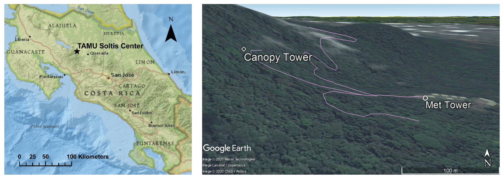
The field site is located at the Texas A&M University Soltis Center near San Isidro de Peñas Blancas in Costa Rica (${\mathrm{10}}^{\circ }{\mathrm{23}}^{\prime }{\mathrm{13}}^{\prime \prime }$ N, ${\mathrm{84}}^{\circ }{\mathrm{37}}^{\prime }{\mathrm{33}}^{\prime \prime }$ W; about 600 m above sea level) (Fig. 1). It shares a boundary with the Children’s Eternal Rainforest. This area has a mean annual temperature of 24 ^∘C, relative humidity of 85 %, and precipitation of 4200 mm (Teale et al., 2014). The study area is classified as a moist, tropical pre-montane forest. The canopy height ranges from 24 to 45 m and is located on a steep eastern slope (Aparecido et al., 2016; Jung, 2009). Rainfall is frequent, and a little over two-thirds of days have one or more rain events. The dry season starts from January and continues until April, and the mean rainfall is about 195 mm per month. The wet season is from May until the end of the year: the average rainfall in the wet season is approximately 470 mm per month (Teale et al., 2014; Aparecido et al., 2016).

Figure 1 The map of the study site and the locations of the two towers (Andrews, 2016).

2.2 Micrometeorological measurements

The site has two primary biometeorological measurement locations (Fig. 1). The main weather tower (hereafter called the “met tower”) is located in a flat, grass-covered clearing at the base of the mountain. The walk-up canopy access tower (hereafter called the “canopy tower”) is located within the forest, on the eastern slope. The met tower measures meteorological conditions without the influence of canopy processes and structure. Precipitation (mm; TE525, Campbell Scientific, Logan, UT), incoming solar radiation, net radiation (W m⁻²; CNR1, Campbell Scientific), air temperature (^∘C; HMP60, Campbell Scientific), and relative humidity data (%; HMP60, Campbell Scientific) have been collected since 2010. The canopy tower has collected the same variables as the met tower (with exception of precipitation). A suite of additional measurements, including greenhouse gas concentrations and fluxes, soil moisture, leaf wetness, and sap flow, have been collected at the met tower since 2014. An infrared, trace-gas profile system (AP200, Campbell Scientific, Logan, UT) and an eddy-covariance system (LI-7200, LI-COR, Lincoln, NE; CSAT3, Campbell Scientific, Logan, UT) are used to collect micrometeorological data at various heights, including concentrations and fluxes of vapor (i.e., H₂O) and carbon dioxide (i.e., CO₂), wind speed and its direction, and air temperature. Additional data are also collected to track canopy processes: leaf wetness sensors at four different heights (LWS, Decagon Devices, Utah), photosynthetically active radiation (PAR) profiles (LI-190, LI-COR) at five heights, leaf area index (LAI) profile using a lined PAR sensor (LI-191, LI-COR) and Beer–Lambert law (Appendix A), leaf temperature sensors for sunlit and shade leaves (SI-111, Apogee Instruments, Logan, UT), soil heat flux (HFT3, Campbell Scientific), soil temperature (5TE, Decagon Devices, WA), soil moisture (EC-4 and 10HS, Decagon Devices, WA), soil respiration (LI-8100A, LI-COR), and transpiration from the sap-flow system. Aparecido et al. (2016) and Andrews (2016) present more detailed information about the sap-flow system and the profile measurements, respectively. The datasets for this site, from 2014 to 2017, are available via the OAKTrust repository (Miller et al., 2018a, b, c, d).

While the canopy tower exceeds the average canopy height, some known interference is present from a nearby emergent tree (Fig. 2), leading to a large gap in the canopy between heights of roughly 30 and 40 m. This configuration leads to two main challenges. Above the gap, the upslope tree (emergent tree) provides a significant degree of shading, which leads to a 70 % reduction in PAR between measurements at the downslope canopy surface (32 m) and above the emergent tree (44 m). We also note that this configuration makes the eddy-covariance method less than ideal. However, the sonic anemometer and infrared gas analyzer (IRGA) are located at 33 m of height, extending away from the tower and clear of obstructions in both the upwind and downslope directions (Fig. 2). As shown in Figs. 1 and 2, predominant winds flow parallel to the valley (N–S) and not perpendicular to this eastern mountain slope. This configuration allows us to capture fluxes, albeit under a narrowed set of ambient conditions. Thus, these data are not necessarily sufficient for recording long-term, integrated measures of ecosystem-level variables, like gross primary production. However, they are suitable for testing and validating models, despite the heterogeneous structure created by the emergent tree.

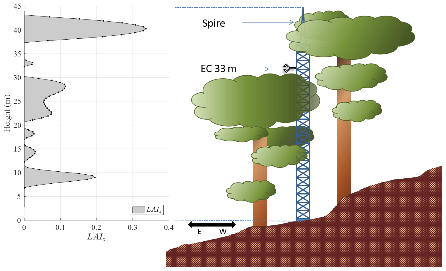
Figure 2 Sketch of the canopy tower located in a plot within a mature pre-montane moist tropical forest in Costa Rica (right) with LAI profiles highlighted (left) along with the location of the eddy-covariance system (EC, 33 m) and the spire (44 m), which holds the net radiometer. The leaf area index is given at 22 discrete points (100 points by spline interpolation) in the canopy (LAI_z), and its sum (LAI) is equal to 6 m² m⁻² for this stand. The LAI_z was estimated based on light profile data and the Beer–Lambert law (Vose et al., 1995). The method for measuring and deriving LAI_z is explained in Appendix A.

2.3 Model description

In this section, we briefly describe CLM's structure and its formulation of the energy balance equation. Given the site's extremely high humidity and annual precipitation, we hypothesize that the sub-models related to water fluxes are the main sources of prediction errors, and as such, the discussion focuses primarily on them. More detailed descriptions can be found in the technical manual (Lawrence et al., 2018; Oleson et al., 2013, 2010). Hereafter we use CLM in a general sense, applicable to both CLM4.5 and CLM5, but provide the specific version number when distinguishing their respective behavior or the effects of recent code modifications.

CLM calculates the radiative transfer through the canopy and the ground surface using the two-stream approximation method (Dickinson, 1983; Sellers et al., 1992; Bonan, 1996; Oleson et al., 2013), which is a starting point for land surface models to determine the exchange of energy. In the procedure, the canopy structure (e.g., LAI, leaf angle) and the current conditions (e.g., wetness, solar angle) are main controllers to determine the absorptivity of incoming solar radiation (albedo). Based on the absorbed incoming energy, fluxes of sensible heat, latent heat, and soil heat are estimated using the energy balance equation. For example, the canopy energy balance can be written as a function of vegetation temperature (T_v):

$$\begin{array}{}\text{(1)}& -S_{\mathrm{v}}+L_{\mathrm{v}}\left(T_{\mathrm{v}}\right)+H_{\mathrm{v}}\left(T_{\mathrm{v}}\right)+{\mathrm{LE}}_{\mathrm{v}}\left(T_{\mathrm{v}}\right)=\mathrm{0},\end{array}$$

where S_v is the absorbed solar radiation by the canopy, L_v is the longwave radiation emitted by the canopy, H_v is the sensible heat flux, and LE_v is the latent heat flux from the canopy, all of which are given in watts per square meter (W m⁻²) (Oleson et al., 2013). Monin–Obukhov similarity theory (MOST) is used to determine resistances along the soil–plant–atmosphere continuum (Fig. 3), which is then used to calculate H_v and LE_v (Zeng et al., 1998; Oleson et al., 2013). Using a big-leaf model, CLM represents both sunlit and shaded leaves (Dai et al., 2004).

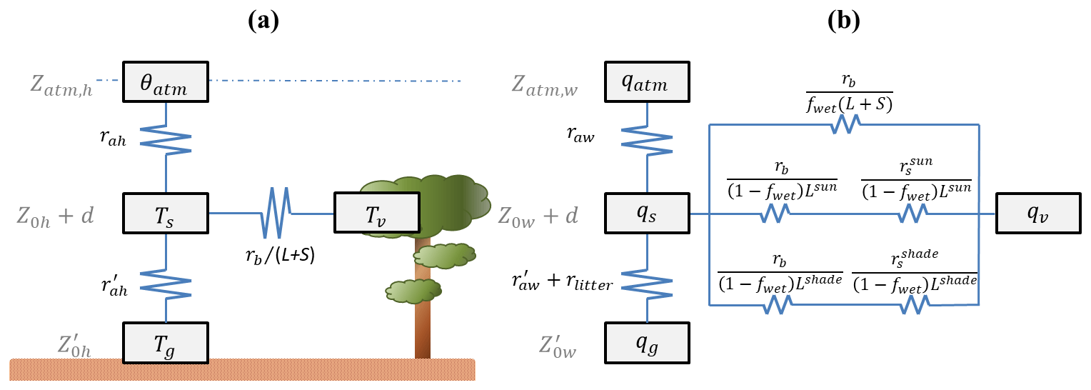
Figure 3 Resistance network schemes incorporated within CLM for (a) sensible heat flux and (b) latent heat flux. Main state variables are atmospheric potential temperature (θ_atm) and specific humidity (q_atm), canopy air temperature (T_s) and specific humidity (q_s), leaf temperature (T_v) and its corresponding specific humidity (q_v), and ground temperature (T_g) and its corresponding specific humidity (q_g). Relevant heights are the atmospheric reference height (z_atm), the canopy roughness height (Z₀), the groundwater roughness height ($Z_{\mathrm{0}}^{\prime }$), and the displacement height (d). Resistances are specified by their scalar (h for heat and w for water vapor), type (a for aerodynamic, b for boundary layer, s for stomatal, or litter for litter), and lighting (sun or shade). Leaf wetness also exerts a control on fluxes via a wetness fraction (f_wet), and (L+S) is the leaf and stem area index. Figure adapted after Oleson et al. (2013).

The water balance equation tracks water flows through the system and connects to the energy balance via its dual controls on ET. The first of these controls, the influence of soil moisture on stomatal conductance, is not considered in this study. Soil moisture does not appear to limit stomatal conductance in the model; the predicted average value of the transpiration wetness factor in CLM was typically around 95 % in this study period and never fell below 50 % for any 30 min time period. Also, prior work has determined that ET at the present study site is not limited by soil water deficits during normal to above-normal rainfall years, such as the period from 2014 to 2016 (Andrews, 2016). On the other hand, leaf wetness can have an influence on this site. While its effect is considered to be small in some ecosystems (Burns et al., 2018), previous studies have shown that leaf wetness exerts a significant influence on fluxes from rainforests in general (Loescher et al., 2005; Kume et al., 2011) and at this site specifically (Aparecido et al., 2017; Moore et al., 2018). CLM reflects these mechanisms as well in the resistance network (Fig. 3b), and the leaf wetness can prevent transpiration and contribute to canopy evaporation rates. Here, leaf wetness is determined by the interception rate of incoming precipitation (Deardorff, 1978; Dickinson et al., 1993; Lawrence and Chase, 2007). The amount of interception q_ic is given in CLM4.5 as

$$\begin{array}{}\text{(2)}& q_{\mathrm{ic}}=\mathrm{0.25}\cdot q_{\mathrm{rain}/\mathrm{snow}}\cdot [\mathrm{1}-e^{-\mathrm{0.5}(L+S)}],\end{array}$$

and in CLM5 as

$$\begin{array}{}\text{(3)}& q_{\mathrm{ic}}=\mathrm{1.00}\cdot q_{\mathrm{rain}/\mathrm{snow}}\cdot \tanh (L+S),\end{array}$$

where q_rain∕snow is the precipitation as liquid or snow, L+S is leaf and stem area index, and 0.25 is a model coefficient. After determining intercepted rainfall, canopy water storage (W_can) is calculated through repartitioning based on the condition of 0≦W_can≦W_max (mm), where maximum canopy water storage (W_max) is 0.1(L+S) (Dickinson et al., 1993; Oleson et al., 2013). Finally, f_wet is

$$\begin{array}{}\text{(4)}& f_{\mathrm{wet}}={\left[{\displaystyle \frac{W_{\mathrm{can}}}{W_{\max }}}\right]}^{\mathrm{2}/\mathrm{3}}.\end{array}$$

Additionally, in CLM5, f_wet cannot exceed a maximum value (f_wetmax) of 0.05. For instance, if f_wet was 0.7, f_wet would become 0.05. Finally, f_dry is calculated as

$$\begin{array}{}\text{(5)}& f_{\mathrm{dry}}={\displaystyle \frac{(\mathrm{1}-f_{\mathrm{wet}})\cdot L}{L+S}}.\end{array}$$

In Eq. (4), the 2∕3 exponent was assumed following the original literature (Deardorff, 1978) because the canopy water tends not to be evaporated when it is set to 1 and evaporates too fast when close to zero (Deardorff, 1978).

Additionally, CLM mainly uses the Farquhar model (Farquhar et al., 1980; Oleson et al., 2013) for photosynthetic rates. At our site, air temperature varies little throughout the year, and CO₂ concentration does not vary significantly. Consequently, light-limited photosynthesis can be considered a dominant process. The light-limited model w_j (µmol m⁻² s⁻¹) in CLM is developed based on the Farquhar model (Oleson et al., 2013) and can be written as

$$\begin{array}{}\text{(6)}& w_j=\mathrm{0.25}{J}_x{\mathbb{C}}_{\mathrm{i}},{\mathbb{C}}_{\mathrm{i}}={\displaystyle \frac{c_{\mathrm{i}}-c_{\mathrm{p}}}{c_{\mathrm{i}}+\mathrm{2}{c}_{\mathrm{p}}}},\end{array}$$

where c_i is the intracellular CO₂ concentration, c_p is the CO₂ compensation point assuming four electrons per CO₂ molecule, ℂ_i is a function of c_i and c_p, and J_x (µmol m⁻² s⁻¹) is the electron transport rate, which can be estimated through

$$\begin{array}{}\text{(7)}& \mathrm{\Theta }{J}_x^{\mathrm{2}}-(I_{\mathrm{PSII}}+J_{\max })J_x+I_{\mathrm{PSII}},J_{\max }=\mathrm{0},\end{array}$$

where Θ is a curvature parameter (Θ=0.7 by default), and J_max (µmol m⁻² s⁻¹) is the maximum rate of electron transport. I_PSII can be estimated as $I_{\mathrm{PSII}}=\mathrm{0.5}\mathrm{\Phi }\cdot I_{\mathrm{APAR}}$, where Φ is the quantum efficiency of photosystem II (Φ=0.85), 0.5 is for two photosystems for one electron, and I_APAR is absorbed PAR (µmol m⁻² s⁻¹).

To further explore these relationships, Eqs. (6) and (7) are simplified and recalculated to make them comparable to the apparent quantum yield (α). This is because the light-limited model has a hyperbolic shape and the shape changes influenced by other environmental conditions. However, the apparent quantum yield is a slope parameter (or the initial slope of the light-limited model) between absorbed PAR and the photosynthetic rate, which is a well-known and simple parameter with a long research history in the literature (Skillman, 2007; Evans, 2013). From Eq. (6), if ambient conditions include $c_{\mathrm{p}}\approx \mathrm{40}\mathrm{\mu }\text{mol}{\text{mol}}^{-\mathrm{1}}$, c_a≈400, and $c_{\mathrm{i}}/c_a\approx \mathrm{0.7}$, then $c_{\mathrm{i}}\approx \mathrm{0.7}\cdot \mathrm{400}\mathrm{\mu }\text{mol}{\text{mol}}^{-\mathrm{1}}$ (Launiainen et al., 2011; Katul et al., 2010) and ℂ_i becomes 0.667. If c_i becomes higher as atmospheric CO₂ concentrations increase, it will approach 1. Through Eqs. (6) and (7), the initial quantum yield of CO₂, also known as the apparent quantum yield (α), can be estimated via $\partial J_x/\partial I_{\mathrm{APAR}}\times \mathrm{0.667}\times \mathrm{0.25}$, which can be used with simple models such as $w_j=\mathit{\alpha }\cdot I_{\mathrm{APAR}}$. It is worth noting that the differential has brought independence from J_max at zero APAR, which is highly related to nitrogen and leaf temperature. The theoretical maximum for α should be ≈0.11; α in saturated conditions is approximately 0.075 (absence of photorespiration), and in normal atmosphere conditions α is about 0.05, which is estimated if Φ≈0.6 in Eq. (7) (Evans, 2013; Raj et al., 2016; Skillman, 2007). These light-limited models with different parameters are explored with observations in a later section.

2.4 Simulation setup and comparison method

CLM was tested in point-scale mode and the satellite phenology (SP) mode with default settings, with exceptions noted below. Extension modes, which consider additional processes such as dynamic global vegetation (DGVM), biogeochemical cycles (BGC), or carbon–nitrogen cycling (CN), were in general not considered since they do not affect our study interests here (e.g., tree growth and stand competition). Input parameters for the simulation were determined using the mksurfdata_map utility provided in the Community Earth System Model (CESM). The utility derives its values from satellite-based global datasets of phenology, soils, and topography provided by University Corporation for Atmospheric Research (UCAR) (Oleson et al., 2013).

Based on multiple initial tests, we decided to use default parameters from the global surface data for our model, as varying them had no significant influence on model performance. Location-specific default parameters from the global dataset include leaf area index (LAI, 5 m² m⁻²), stem area index (SAI, 0.8 m² m⁻²), canopy height (34 m), sandy clay loam soil (47 % sand, 26 % clay, 27 % silt), organic matter density (33 kg m⁻³), and color class (15). We need to note that default CLM cannot yet reflect leaf area density (LAD) as in Fig. 2. Changing any of these parameters from the global values to local values did not significantly affect the model’s results in our tests. This is perhaps because our LAI value is high enough to be the dominant parameter, and the role of the soil is small. Moreover, the slope parameter exists in the model, but it is not actually used in CLM's radiative transfer, canopy process, and turbulence sub-models. Additionally, most of the measured parameters at this site were not very different from the default values. Therefore, we decided to use the default setting except for some significant differences as outlined below. The tropical broadleaf evergreen tree (BET) plant functional type (PFT) was used as the basis for representing the site's specific land cover. The location in question had a default value of 30 % BET tropical, 30 % tropical broadleaf deciduous trees (BDT tropical), and 25 % grass and crops, which we altered to 100 % BET for purposes of this study. The atmospheric reference height was set to 44 m to reflect the location of the net radiation sensor on the canopy tower.

As an input, a meteorological forcing dataset for CLM was created based on the measurements collected on-site. These variables included half-hourly averages of wind speed (m s⁻¹), incoming solar radiation, relative humidity, air temperature, air pressure, precipitation, and CO₂ concentration. Comparison of the simulation was based on measurements taken at the canopy tower; thus, canopy tower data were primarily used as forcing data when data were available. Average precipitation and air temperature data collected at 10 m of height at the met tower were also used for gap-filling. In most cases, weather data obtained from the two towers were highly correlated, as the locations are less than 1 km apart and only differ in their immediate surroundings (i.e., forest vs. clearing) and slope degree (i.e., ∼45^∘ slope vs. flat terrain).

Although flux methods cannot measure gross primary production (GPP) directly, it is an extremely important variable in the context of global carbon cycle modeling. In light of this, we estimated GPP based on net ecosystem exchange (NEE), net ecosystem production (NEP), and ecosystem respiration (ER), where NEE ≈ NEP and GPP = NEP – ER. With eddy-covariance data collected at the height of 33 m, NEP was estimated as CO₂ flux + CO₂ storage flux. Ecosystem respiration (ER) was estimated to be around 1.2 (µmol m⁻² s⁻¹) based on the nighttime data found using the u^* threshold method (Papale, 2006; Reichstein et al., 2005). These EC-based data for the CO₂ and H₂O flux can still be questionable due to the instrument configuration. However, comparison of the EC data and sap-flow data (discussed below) showed acceptable similarity, and these data were accurate enough to give information on whether the model has a significant error.

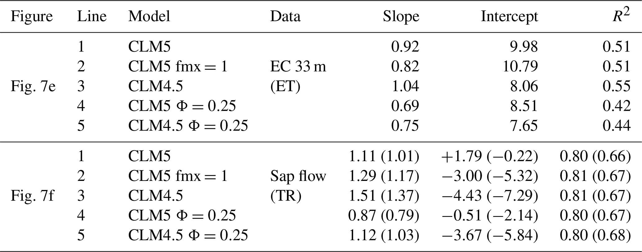
For transpiration (TR), measured data and simulated transpiration rates are compared at daily timescales. For the comparison, it is necessary to estimate or measure each major flux (partitioned flux) within ET. At this site, upscaled sap-flow data provide a transpiration rate (Aparecido et al., 2016), which in turns allows for water vapor flux partitioning. Although the sap-flow data at the site tend to lag temporally and nocturnal sap flow occurs (shown later), it provides data to be used for comparison at a daily scale against CLM estimates. As CLM cannot represent nighttime transpiration, the nighttime sap-flow data, collected when the cosine zenith in CLM is less than zero, were eliminated from the comparison. However, taking into account the fact that the nighttime sap-flow rate possibly occurs to recharge the sap water, an additional comparison was made without the elimination of nighttime value. This daily-scale comparison is made by a one-to-one figure with R-squared values. Also, regression analysis provides additional information on how much the model deviates from observations, as a slope of 1 and an intercept of 0 are expected from model–measurement comparisons. We note that the intercept is related to the daily average value, and it should be directly affected by the elimination of the nighttime transpiration; a portion of this difference is related to the lag.

Unlike radiative transfer models, CLM5 notably updated from CLM4.5 the physiological models for GPP and TR as well as their associated parameters. The Ball–Berry model (BB) (Ball et al., 1987) was supplanted by a combination of the Medlyn model for the stomatal conductivity (Medlyn et al., 2011), a plant hydraulic stress model (Bonan et al., 2014), and the Leaf Use of Nitrogen for Assimilation (LUNA) routine (Ali, 2016). For the stomatal conductivity, regardless of the type of model (BB or Medlyn model), the slope parameter, which links stomatal conductivity and carbon fixation (i.e., photosynthesis), has been reduced by the model update. While the BB model can still be used for CLM5, its slope parameter has been changed from 9 to 7.3 for C₃ plants. We have tested several options in CLM5 and determined that changing the stomatal conductivity model does not affect photosynthesis-related results (e.g., GPP) in our case.

To facilitate comparisons, CLM requires assigning the height of each output variable. In this case, each reference height was determined based on given parameters in CLM: the displacement height was d=23.45 m, ground roughness height was $z_{\mathrm{0}\mathrm{mg}}=z_{\mathrm{0}\mathrm{qg}}=z_{\mathrm{0}\mathrm{hg}}=\mathrm{0.01}$ m, and surface height was $z_{\mathrm{0}}=z_{\mathrm{0}\mathrm{mv}}=\mathrm{2.625}$ m, so the canopy height became $d+z_{\mathrm{0}}=\mathrm{26.075}$ m. For instance, canopy air temperature (T_a) in CLM was 2 m temperature in this comparison study, and it was $d+z_{\mathrm{0}}+\mathrm{2}=\mathrm{28.075}$ m. CLM uses the T_s term in Fig. 3, which refers to canopy air temperature, but the CLM module does not provide T_s values as one of the output variables. This 2 m temperature (T_a), called TSA in CLM outputs, would be the closest available value from the canopy. Moreover, our profile data indicate that air temperature does not vary much at different heights near the top of the canopy, and 28.075 m is still within the canopy. Our instrument heights did not exactly correspond to those heights from CLM, so the nearest one or two data points were used for the comparison rather than interpolating all data.

Additionally, CLM5 has a low default leaf wetness ratio; the maximum is 0.05 as in Eq. (4). For fair comparison, all leaf wetness values from CLM were normalized to a [0–1] scale based on the water amount on the canopy using Eq. (4). Additionally, the question of whether or not to apply the power of 2∕3 did not change our comparison results significantly.

Soil-related data were spatially upscaled and vertically interpolated to compare with the simulation. For the spatial upscale, soil temperatures and soil heat fluxes were measured at five different places near the canopy tower, and the vertical profile data were also collected close to the base of the tower. For the vertical profile, CLM considers a larger number of soil layers. Therefore, the results of CLM were linearly interpolated to compare with the measured data.

To initialize the simulations, CLM was first executed with a cold start (i.e., randomly produced initial values) and run for 100 years to get stable soil temperatures, cycling (through) the 6-year forcing data collected between the beginning of 2010 and the end of 2015. Once stable soil temperatures were obtained, CLM was rerun for 2 years (2014–2016) at a 30 min time step. For some cases, linear regressions were performed to compare CLM outputs to field data. The goodness of fit of the regression analysis was determined based on coefficient of determination (R squared) where appropriate. In this analysis, we focused on the following variables: net radiation, PAR, albedo, CO₂ flux, GPP, transpiration, latent heat flux, air temperature, leaf temperature, leaf wetness, and soil-related variables. We additionally tested how changes in levels of maximum leaf wetness (f_wetmax) and the quantum efficiency of the photosystem (Φ) affected the goodness of fit. Modifications of LAI, light-extinction-related coefficients, and canopy heights (34–44 m) were also tested. Unlike f_wetmax and Φ, however, they provided no significant difference or better results, so comparison and discussion of them are not made here.

3 Simulation results and comparison

3.1 Net radiation and albedo

A comparison of light-related variables indicated that the simulated land surfaces received less energy than field measurements, but the difference was not significant. Simulated net radiation values were 20 W m⁻² less than the average measured values, although diurnal patterns closely matched (R²=0.99). Net radiation in CLM was approximately 15 to 45 W m⁻² lower than field measurements during the daytime and 10 to 15 W m⁻² lower during the nighttime (Fig. 4a, b). Little difference (<5 W m⁻², R²=0.99) was detected between CLM4.5 and CLM5. The simulated shortwave reflectance (albedo) in CLM was around 15 % higher than the gauged albedo (+0.022 across all daytime data) (Fig. 4c), which likely caused the differences in daytime net radiation.

Light data were clearly affected by the sloped terrain. Although the models were developed for all the global surface, sub-grid-scale heterogeneity in land surface elevations has not yet been implemented in CLM4.5 and 5.0. Albedo from CLM tended to have a symmetric form, while the measured albedo had a skewed diurnal pattern (Fig. 4c). This skew caused a noticeable discrepancy with the modeled values in the early morning, which peaked during midafternoon (+0.0517 at 15:00; Fig. 4c). The highest PAR intensity (or highest incoming solar radiation) occurred at 10:00 (Fig. 4e) when the albedo difference between the observations and the simulation was smallest (+0.0214). In some parts, this may be caused by albedo models that are too simple, which cannot properly respond to the intensity of solar radiation and angle. However, the skewed albedo seen in the measured data in Fig. 4c and d clearly indicates that CLM cannot represent the slope effect of the land surface. Such skewed diurnal variations were also observed in the PAR profiles (Fig. 4e, f). The measured PAR values, generated by sensors somewhat shaded by the upper canopy, were diurnally skewed compared with shaded PAR from CLM. In contrast to the solar radiation above the canopy (i.e., the top of the tower, net radiation), the radiation profile started to become skewed right after infiltrating the top canopy layer. When revisiting the effect of canopy gaps created by the emergent tree, we observed that radiation values between the top of the canopy (≈400 W m⁻² at 44 m from net radiation) and the next nearest heights (≈110 W m⁻² at 32–38 m from PAR) were considerably different (about 70 %–80 % reduction from the top), as mentioned before. The height of the primary canopy, consisting of the dominant trees, is about 38 m (Aparecido et al., 2016). Therefore, the shade effect (optical thickness) may be substantial, even though the emergent trees added minimal thickness. This feature can be important because the hillslope surface is more sensitive to the sun angle, which affects the sunlit–shaded area ratio.

Simple manipulation was attempted by changing the solar angle to mimic the slope effect on albedo (Fig. 4c, d, e). The cosine zenith angle in the two-stream approximation was reestimated by pushing back 30^∘ to apply to the light extinction coefficient K in the two-stream approximation. This simple modification reduced some of the skewness of the albedo (Fig. 4d). However, shaded PAR showed opposite behavior compared to the observation, mainly because sunlit area was increased.

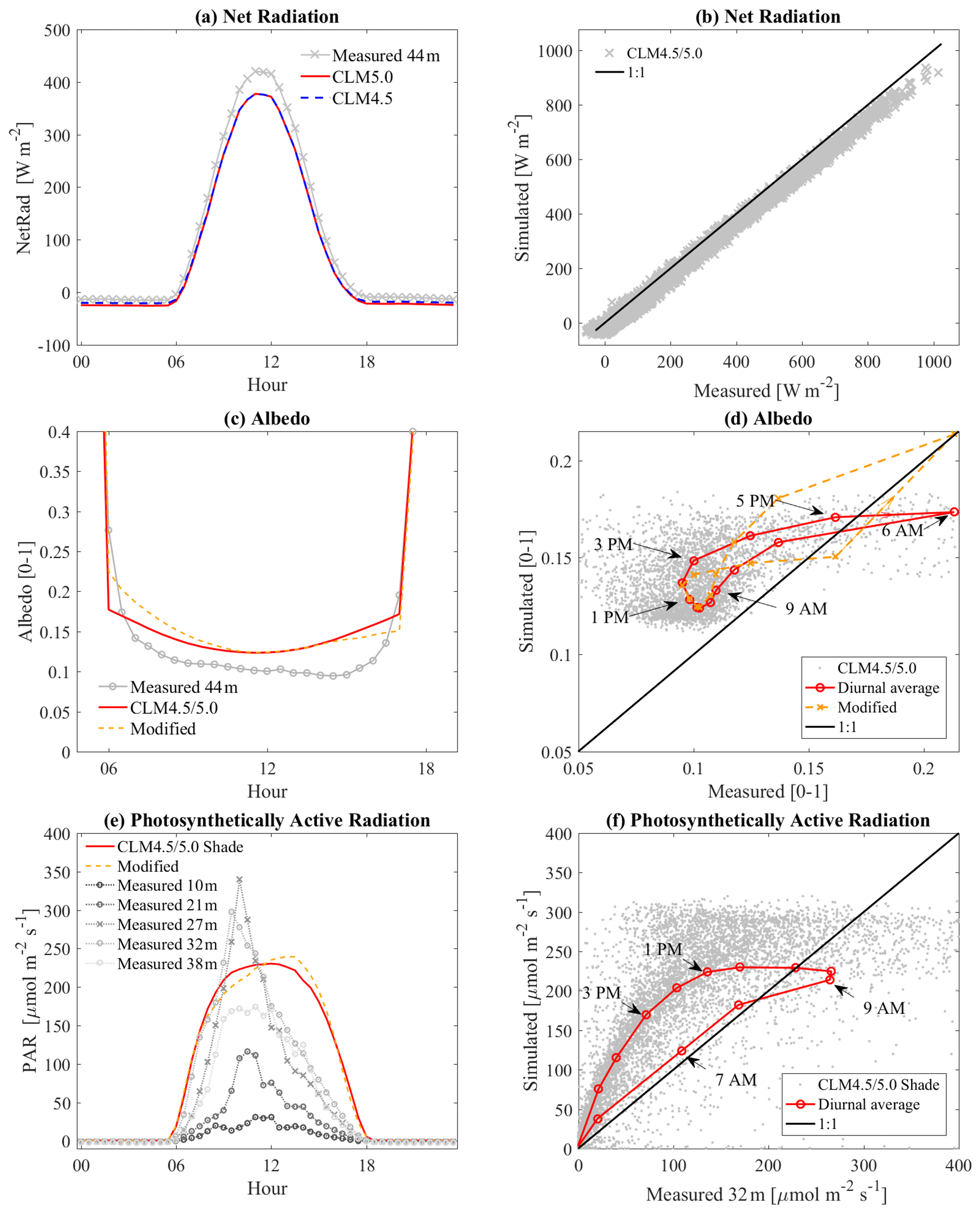
Figure 4 (a, b) Comparison of net radiation between CLM and measurements on the canopy tower at 44 m. (c, d) albedo at 44 m. (e, f) PAR comparison for shaded canopies. All left plots (a, c, e) are ensemble diurnal variation, and the right plots (b, d, f) are one-to-one comparison plots between CLM and measured data. Hysteresis depicted in (d) and (f) is based on hourly ensemble average values for daytime. “Modified” is an attempt to mimic the slope effect with a simple update of the two-stream approximation.

3.2 CO₂ flux (GPP)

All CLM versions (CLM4.5, CLM5, and CLM5BGC) overestimated GPP (6.7, 4.9, and 3.6 µmol m⁻² s⁻¹) (Fig. 5a, b). Results from the new version, CLM5, were generally more similar to the measured data than those in CLM4.5 (Fig. 5a). CLM5 yielded lower photosynthetic rates than CLM4.5, possibly due to the lower BB slope parameter and also due to suppressed maximum rates of V_c, max25 and J_max25 by the LUNA and BGC mode. Inactivating the plant hydraulic stress model in CLM5 increased the carbon assimilation rate, while disabling the LUNA model decreases it in this site study. The prediction for the middle range of the photosynthetic rate (5–15 µmol m⁻² s⁻¹) did not improve much compared with CLM4.5.

One of the possible causes of the discrepancy between the estimated GPP and its observed values may be the model determining the response to light limitations (Fig. 5b). Comparison between absorbed PAR (APAR) versus GPP shows that the initial slope of measured data is much lower than the simulated one (Fig. 5c). The APAR, including sunlit and shade leaf area, was estimated in CLM using measured incoming solar radiation above the canopy at 44 m. As previously explained (Fig. 5d), an extensive literature study by Skillman (2007) and Evans (2013) showed the theoretical maximum for α should be ≈ 0.11, that α under saturated conditions is approximately 0.075 (absence of photorespiration), and that in normal atmospheric conditions α is about 0.05, which is estimated when considering Φ≈0.6 in Eq. (7) (Evans, 2013; Raj et al., 2016; Skillman, 2007). From our observations, the fitted value for α was 0.021 (Φ≈0.25). This low value may have been caused by other factors such as physiological stress or a scale problem. The fitted value was estimated from eddy-covariance measurements rather than at the leaf scale. By default, α is around 0.07 in CLM4.5 and CLM5, with ℂ_i=0.667, which is higher than 0.05 as usually reported (Skillman, 2007; Ehleringer and Pearcy, 1983; Ehleringer and Björkman, 1977). Of course, this method itself has a possible error caused by the issues inherent in the eddy-covariance measurements, as well as the estimation of APAR in CLM, which contains only sunlit and shade leaf area, making it too simplistic. For this study, Φ was modified to produce an appropriate value for α, but the issue should be revisited in future studies.

Test simulations with CLM4.5 and CLM5 were conducted using Φ=0.25 and Θ=0.7. When Φ was updated, both CLM4.5 and CLM5 performed better than before (Figs. 6, 5a). This change resulted in more stable predictions, as judged by the middle range of GPP (5–15 µmol m⁻² s⁻¹). Maximum GPP was reduced as expected (Fig. 5d), and it was possible to further fix such an over-reduction by updating Θ (curve shape), as shown on Fig. 5d. The change in the slope can alter the maximum assimilation rate, and the alteration can be counterbalanced if Θ is modified. In the simulated diurnal variation plot, the trend was slightly shifted in the afternoon, also probably due to the effects of the topographical slope (Fig. 6b). Time-dependent classification (i.e., regression lines with the intercept forced through zero; Fig. 6b) and the fitted slopes indicated that geographical features have an influence on photosynthetic activity, which is mostly caused by the radiative transfer models, like albedo. However, the model failed to accurately represent such features, since the CO₂ flux in CLM was lower in the morning and higher in the afternoon.

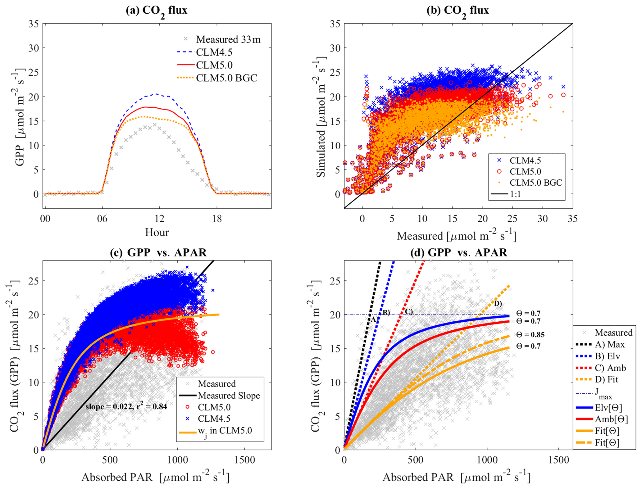
Figure 5 (a) Ensemble diurnal variation of the CO₂ flux: differences between eddy covariance (canopy tower 33 m) and CLM in daytime are 6.7, 4.9, and 3.6 µmol m⁻² s⁻¹ for CLM4.5, CLM5, and CLM5BGC, respectively. (b) Scatter plot using data shown in previous panel with one-to-one line noted (a). (c) APAR vs. GPP, and w_j is simulated with default parameters and ℂ_i=0.667. (d) The light-limited model tested with different parameters. “Max” is the theoretical maximum, “Elv” is saturated–elevated conditions, “Amb” is normal atmosphere conditions, and “Fit” is a fitted value from our observations. In the legend, [Θ] means the usage of the hyperbolic function in Eq. (7), like Elv[Θ]. Without [Θ], only the slope parameter is active as “Elv”. These parameters are described in full in Sects. 2.3 and 3.2.

Figure 6 Test simulation using Φ=0.25 and Θ=0.7 as in Fig. 5d. By the modification of Φ, maximum GPP has been reduced. It is possible to improve this model by updating Θ; r² is an R-squared value without an intercept. The units for both (a) and (b) are the same (µmol m⁻² s⁻¹).

3.3 H₂O flux

The effect of the change in f_wetmax was detected in the model's results for vapor fluxes (Fig. 7). Again, CLM5 has a low leaf wetness coefficient (i.e., the maximum rate is 0.05 as in Eq. 4, which reduced canopy evaporation and elevated the transpiration rate). In this simulation, f_wetmax was considered to be 1 for CLM5 (hereafter referred to as CLM5 fmx =1), and we used this when we wanted to make a fairer comparison with CLM4.5

Similarly to the CO₂ flux, total H₂O fluxes of CLM5 were overestimated (2.1 × 10⁻⁵ mm s⁻¹ higher in daytime than eddy-covariance values). Flux rates in the CLM5 fmx =1 simulations were reduced in comparison to those predicted by CLM4.5 (Fig. 7a, b). The notable decrease (CLM4.5 and CLM5 with Φ=0.25) was due to the change in the quantum yield (α) parameter needed for GPP predictions (Fig. 6). Transpiration rates (TR) also showed similar trends, and this indicates that TR is an important process at this site.

At the daily timescale, CLM4.5 produced the highest estimates for both ET and TR in comparison to the other versions (Fig. 7e, f). CLM5 yielded a notable reduction of ET and TR due to the newly implemented leaf wetness parameter f_wetmax. We can visually determine that applying a quantum efficiency of Φ=0.25 made fitted lines closer to the 1:1 line for both ET and TR (Fig. 7e, f). However, we cannot conclude that it was improved, since although the low Φ changed the slope and intercept values it did not change the R-squared values significantly. This change might also be influenced by other components such as leaf wetness. Here, correlations of TR were slightly increased by around 0.01 ($R_{\mathrm{CLM}\mathrm{4.5}}^{\mathrm{2}}$ = 0.67, $R_{\mathrm{CLM}\mathrm{5}}^{\mathrm{2}}=\mathrm{0.68}$) when considering Φ = 0.25. On the other hand, the correlations of ET were decreased by around 0.1 ($R_{\mathrm{CLM}\mathrm{4.5}}^{\mathrm{2}}=\mathrm{0.42}$, $R_{\mathrm{CLM}\mathrm{5}}^{\mathrm{2}}=\mathrm{0.44}$) (Table 1). When assuming a lower quantum efficiency, the change in TR makes the fitted slope for ET decrease (Fig. 7e), possibly since transpiration is a more influential component than evaporation at this site. Thus, TR drove ET rates when there were higher energy exchange conditions (i.e., warm, sunnier, and drier time). On the other hand, these results also highlighted the importance of other sub-models such as canopy evaporation.

Figure 7 (a) Ensemble diurnal variation of the total H₂O flux; “measured 33 m” is measured by eddy covariance (at 33 m), “sap flow” is transpiration measured through sap flow, all CLMs are about evapotranspiration (ET), fmx =1 represents fwetmax =1, and Φ=0.25 means 0.25 applied to Φ in Eq. (7). (c) Partitioned H₂O flux, where ET, TR, and VE are evapotranspiration, transpiration, and canopy evaporation from CLM; (b, d) the one-to-one plots of (a) and (c). (e, f) Daily ET and TR (except nighttime) against eddy-covariance and sap-flow data.

Table 1 Fitting parameters and regression coefficients for sap-flow and eddy-covariance measurements versus simulations by CLM at a daily scale for Fig. 7e and f. The nighttime data are excluded (set to zero) for both and values in parentheses are with nighttime data (intercept unit: 10⁻⁶ mm s⁻¹).

3.4 Leaf wetness

The leaf wetness fraction predicted by CLM was compared to observations made using capacitance sensors (Fig. 8). In the analysis, the ensemble diurnal variations of leaf wetness were plotted; 38 m, 11 m, and 3 m are the measurement heights, and the others are leaf wetness from CLM5 (f_wetmax=0.05), CLM5 fmx =1 (f_wetmax=1), and CLM4.5 (f_wetmax=1) (Fig. 8b). The predicted leaf wetness was not in agreement with the diurnal leaf wetness variation measured at this site (Fig. 8b). In particular, the nighttime fraction of leaf wetness was significantly higher when compared with gauged data. The biggest problem detected in this study was that intercepted canopy water was rarely evaporated in the model. The canopy water tended to accumulate, especially due to frequent nighttime rainfall that started in the late afternoon or high daytime humidity, which caused condensation. Daytime leaf wetness seems to be reasonably simulated (Fig. 8b). However, no trend could be identified in the comparison between simulated and measured data (not displayed here), which indicated that the formula cannot adequately represent the actual behavior of the wet fraction in both CLM5 and CLM4.5.

Intercepted precipitation was usually too high in CLM compared to observed leaf wetness (Fig. 8c, d). The values in Fig. 8c and d show the increasing rate of leaf wetness due to precipitation, with the large and thick markers indicating their averages. The collected data were conditioned upon the absence of a rainfall event at least 2 h prior and an initial leaf wetness lower than 0.2. Figure 8c shows 0.5 h rainfall events (one consecutive event at a 30 min scale) and Fig. 8d is for 2 h rainfall events (four consecutive events). This increment was directly related to canopy interception: the usual increment for 2 h (and 30 min) rain was 0.71 (0.33) at a 38 m height, 0.48 (0.28) at a 3 m height, around 0.88 (0.73) in CLM5, 0.97 (0.77) in CLM5 fmx =1, and 0.94 (0.46) in CLM4.5. The modified interception model (CLM5 fmx =1) from Eq. (3) resulted in a higher interception rate than CLM4.5 fmx =1 (Eq. 2). The interception rate also seemed higher with CLM5 fmx =1 than with original CLM5 as in Fig. 8c because CLM5 fmx =1 had a higher canopy evaporation rate. This effect resulted in the acceleration of canopy evaporation while allowing interception to play a larger role in the canopy water balance. In the one-to-one comparison, the increase in leaf wetness in CLM was usually higher than in measured data. Consequently, the wet canopy fraction at the beginning of the drying process was usually higher in CLM than in the measurements: 0.63 in the 38 m observation, 0.47 in the 3 m observation, 0.96 in CLM5, 0.9 in CLM5 fmx =1, and 0.78 in CLM4.5 (see y-axis data on the 0 x axis in Fig 7e).

Another analysis showed that leaf wetness behavior is highly sensitive to incoming solar radiation. The water state on a leaf in Fig. 8e and f was tracked over consecutive no-rain events for 3 h right after the last rain events in the daytime between 10:00 and 14:00. Figure 8e shows events with low solar radiation (0–300 W m⁻²) and Fig. 8f shows events when solar radiation was higher than 300 W m⁻². Although it was difficult to gather data for these serial drying events (each plot uses at least 12 groups of six consecutive half-hourly time periods with no rain), the result clearly indicated that leaf wetness is strongly influenced by an increase in incoming solar radiation when f_wetmax=1 (CLM5 fmx =1 and CLM4.5). In the case of f_wetmax=0.05 (CLM5), the drying rate is reasonable at low solar radiation, but it is higher than values observed during high incoming solar radiation. The measured data in the analysis showed relatively smaller values of leaf wetness at lower levels of the canopy. This indicated that rainfall does not frequently reach the lower canopy, and thus interception rates are low there. This finding would suggest that lower f_wetmax values are reasonable.

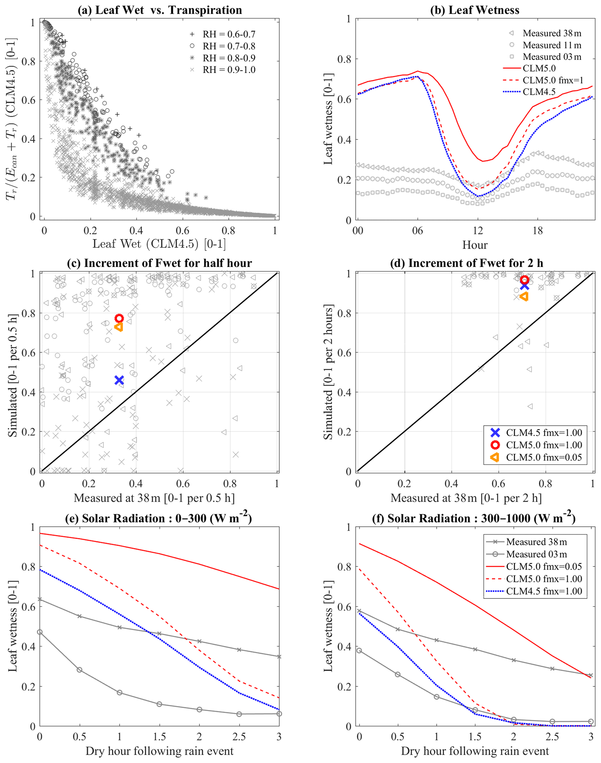
Figure 8 (a) TR ∕ ET versus leaf wetness and classified by relative humidity [0–1]. (b) The ensemble diurnal variation of leaf wetness. Panels (c) and (d) indicate interception rates, and panels (e) and (f) represent the behavior of a drying canopy. The marked lines are from measurements, and lines are estimated from CLM.

3.5 Temperatures and soil flux

The simulated canopy air temperature in both CLM4.5 and CLM5 was overestimated during daytime (+0.8 and +1 ^∘C, respectively) and underestimated during the nighttime (−1.9 and −1.1 ^∘C, respectively) (Fig. 8). In other words, the simulated temperature may be overly sensitive to incoming solar radiation, like leaf wetness, which was overestimated during the day and underestimated at night. The updated MOST scheme improved nighttime air temperatures in CLM5 (Burns et al., 2018), but they were still underestimated. As reported in the previous section, water remaining on the canopy during nighttime tended to be inefficiently evaporated (Fig. 8b), which was also possibly related to low canopy temperature in CLM. At lower canopy levels, the ground air temperature at the surface was overestimated during daytime, and it was even higher than air temperature at heights of 1–5 m (Fig. 9b).

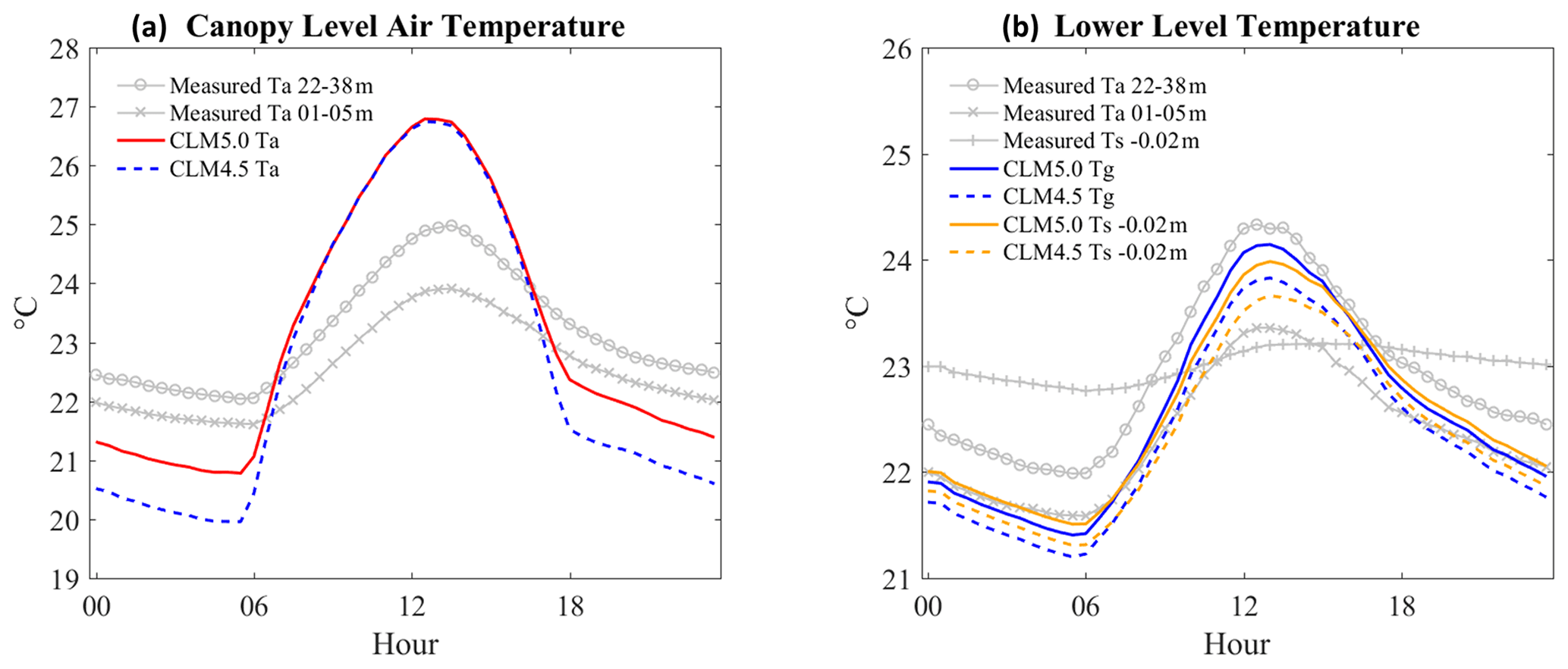
Figure 9 The ensemble diurnal variation of air temperatures. Canopy levels at 22–33 and 1–5 m are measured air temperatures, T_a represents air temperature at 28.075 m in CLM, and T_g is ground air temperature at 0.01 m in CLM. T_s −0.02 m is measured and simulated soil temperature. In (a), both CLM4.5 and CLM5 overestimate in daytime (+0.8 and +1 ^∘C) and underestimate during the nighttime (−1.9 and −1.1 ^∘C). In (b), differences between measured T_a 01–05 m and all CLM values (CLM5.0 T_g, CLM4.5 T_g, CLM5.0 T_s, and CLM4.5 T_s) are −0.39, −0.14, −0.32, and −0.06 in daytime and −0.02, 0.18, −0.11, and 0.08 ^∘C in nighttime. Differences with measured T_s −0.02 m are −0.04, 0.21, 0.03, and 0.30 in daytime and 0.90, 1.10, 0.81, and 1 ^∘C in nighttime.

The ground surface tended to have high energy exchange during daytime, similar to the canopy processes. Considering the soil temperatures (Fig. 9) and the soil heat fluxes (Fig. 10), we found they were overestimated during daytime and underestimated in the nighttime. Soil temperature and heat flux in CLM were highly variable. Soil evaporation rates in both CLM4.5 and CLM5 were also overestimated compared with estimated data from soil respiration chamber measurements (LI8100) (Fig. 10). For daytime soil evaporation, the average difference from the observation was $\mathrm{5}\times {\mathrm{10}}^{-\mathrm{7}}$ mm s⁻¹ with CLM4.5 and $\mathrm{15}\times {\mathrm{10}}^{-\mathrm{7}}$ mm s⁻¹ with CLM5. The measured field value was around $\mathrm{1}\times {\mathrm{10}}^{-\mathrm{7}}$ mm s⁻¹. The simulated soil moisture also had high variability, with low mean water contents (around 0.2 m³ m⁻³) compared with gauged values (0.3–0.4 m³ m⁻³).

The overestimation of vegetation temperature (T_v) in both CLM4.5 and CLM5 also appeared in the daytime simulation ($\approx +\mathrm{1.0}$ to 2.4 ^∘C) (Fig. 11a, b). Another model test was also made using global forcing datasets (Qian et al., 2006) to corroborate our simulations, and the result showed very similar behavior ($\approx +\mathrm{5}$ ^∘C, not depicted here). The high T_v and T_a from CLM simulations resulted in lower relative humidity than gauged-based canopy air humidity. We note that the sunlit–shade scheme in CLM does not consider two different vegetation temperatures, so it only takes a single variable T_v to represent the entire canopy. Canopy temperature (T_v) in CLM should be an average of sunlit and shaded leaf temperature, but the simulated results were far from our expectation (Fig. 11a). A comparison plot also showed significant error (Fig. 11b). The additional comparisons indicate that T_v on sunlit leaves normally followed the canopy air temperature (leaf thermoregulation), but CLM did not reproduce such behavior (Fig. 11c, d).

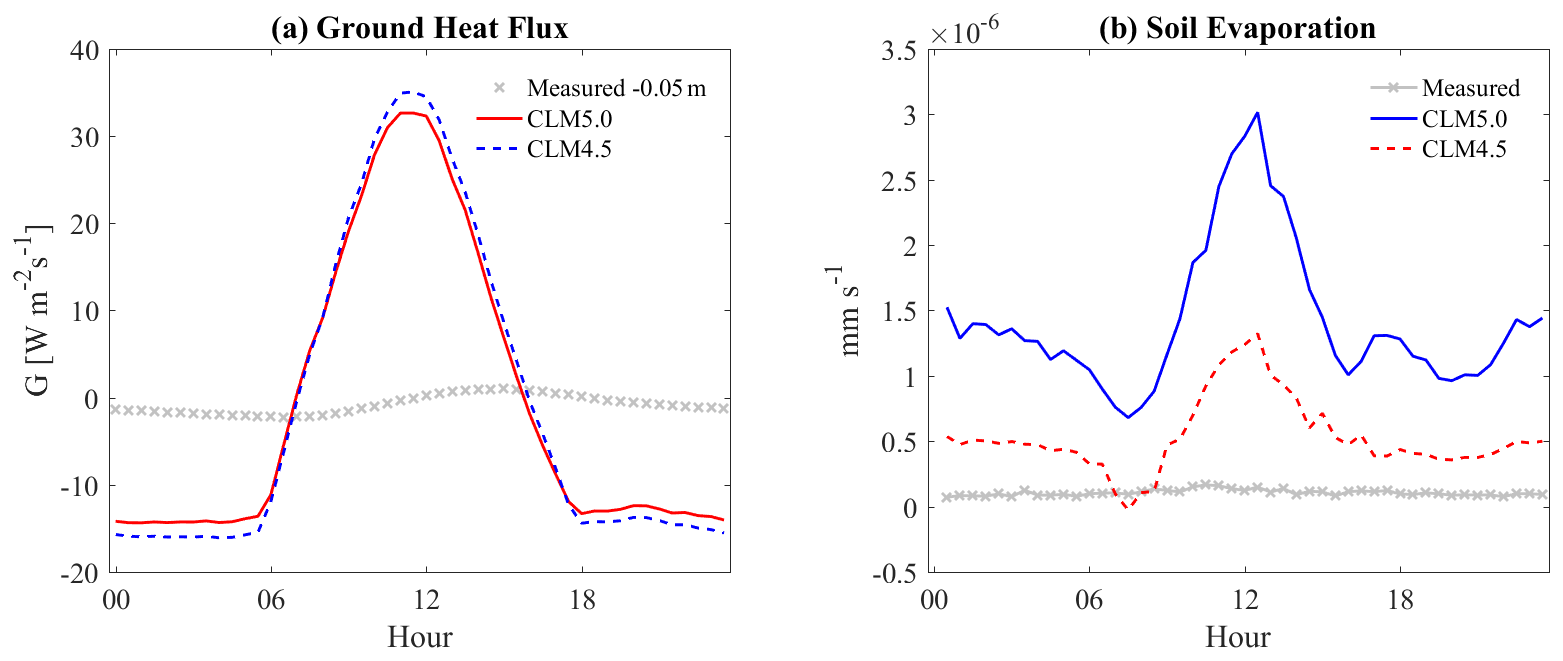
Figure 10 The ensemble diurnal variation of soil–ground heat fluxes (into soil +) (a) and soil evaporation.

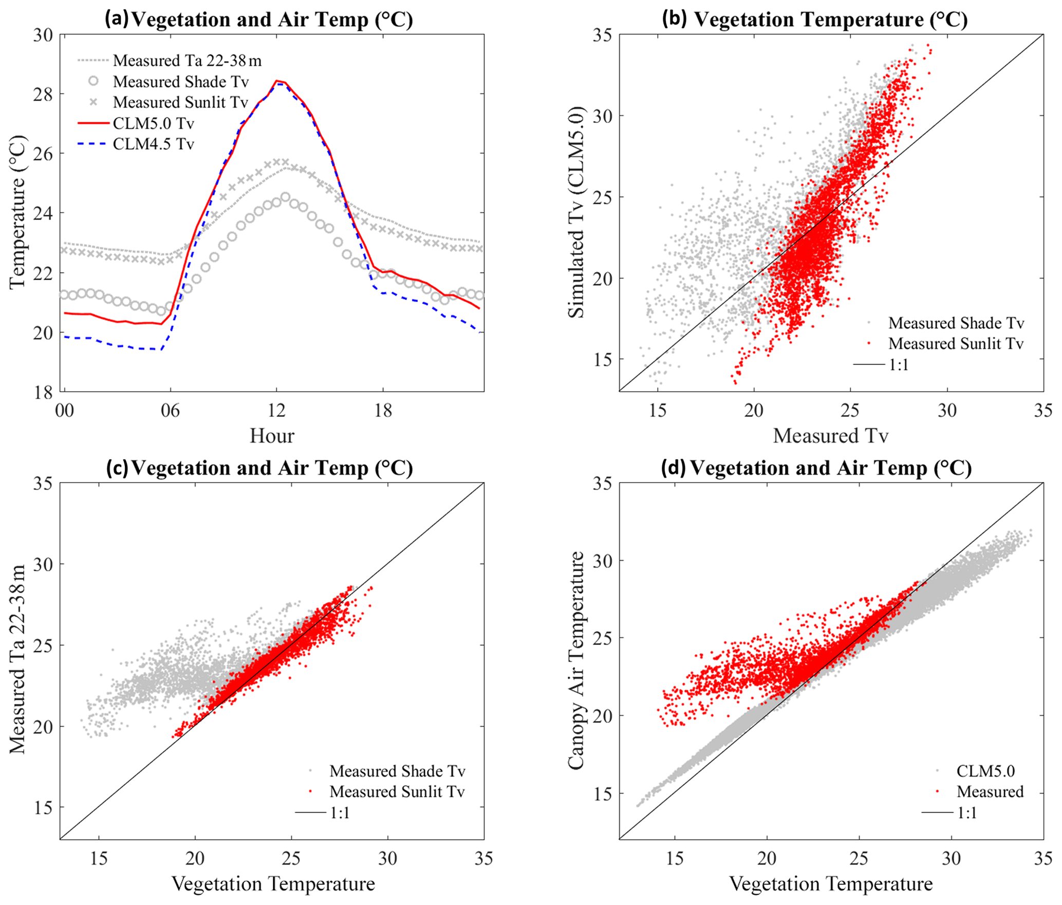
Figure 11 (a) The diurnal variation of leaf temperatures with measured canopy air temperatures. (b) The one-to-one plot of leaf temperatures: CLM vegetation temperatures (T_v) are compared with measured values for the both gauged shade (shade T_v) and sunlit (sunlit T_v) vegetation temperatures. (c) The one-to-one plots for measured canopy air temperatures versus measured leaf temperatures (sunlit and shade). (d) The one-to-one plots for canopy air temperatures versus leaf temperatures from CLM (CLM5 T_a vs. CLM5 T_v) and observations (canopy T_a 22–38 m vs. averaged T_v from sunlit and shade T_v): averaged T_v is estimated through $({\mathrm{LAI}}_{\mathrm{Shade}}\times T_{{\mathrm{v}}_{\mathrm{Shade}}}+{\mathrm{LAI}}_{\mathrm{Sunlit}}\times T_{{\mathrm{v}}_{\mathrm{Sunlit}}})/\mathrm{LAI}$. In panel (a), daytime differences for CLM 5.0 T_v minus measurements (measured T_a 22–38 m, measured shade T_v, and measured sunlit T_v) are 1.1, 2.4, and 1.0. In nighttime, the differences are −2, −0.3, and −1.8 ^∘C. CLM5 is normally 0.2 higher in daytime and 0.8 higher in nighttime.

4 Discussion and conclusions

In this study, two versions of the Community Land Model (CLM4.5 and CLM5), running primarily in the satellite phenology (SP) mode, were tested against measured data from a mountainous tropical rainforest in Costa Rica. Net radiation was underpredicted by an average of −20 W m⁻² (Fig. 4a, b) in both CLM4.5 and CLM5. The discrepancy was attributed to CLM's overprediction of surface albedo, which was on average 0.022 lower in the measurements (Fig. 4c, d).

The effects of topographic slope clearly appeared in the diurnal plots for albedo, PAR (Fig. 4), and theCO₂ flux (Fig. 6). With respect to albedo, the hillslope shading effect magnified these discrepancies, with afternoon values having larger differences as the sun moved behind the north–south-trending mountain (Fig. 4). The level of discrepancy varied according to the diurnal cycle of the intensity of incoming solar radiation and the solar angle (Fig. 4c, d). PAR profiles also showed that radiation levels within the canopy had a skewed, or hysteretic, cycle (Fig. 4e, f), which was not captured by CLM. These results indicated that canopy radiative transfer, including the surface albedo and sunlit–shade separation, may need to be better represented in advanced land surface models in order to simulate a more realistic response to solar radiation or topographical slope. A simple modification of albedo was attempted, but it resulted in an error on other variables such as PAR. The update may require more complicated manipulation to satisfactorily match variables in addition to albedo (e.g., PAR). This finding suggests that a multiple-layer scheme is necessary to properly represent light penetration. More importantly, aerodynamic resistance models, such as MOST, are also currently incapable of representing a sloped terrain. If the effects of both can be implemented in CLM, predictions can be highly improved for mountainous regions, especially if they can be considered at a fine grid scale.

The study found that slope affected various data and outputs to an important degree and suggested that additional observations are necessary to examine and capture such features. Several past studies to compare and improve CLM have taken a similar approach. However, they focused on specific sub-model performance (Burns et al., 2018; Swenson and Lawrence, 2014; Bonan et al., 2011), rather than studying the effects of spatial complexity. For albedo, the slope effects were minor in this study; skewness in the diurnal average curve was relatively small, and it is difficult to identify the difference between measured and modeled net radiation curves. On the other hand, the skewness for PAR is significant, and this was obviously related to the different response of GPP through time (Fig. 6). Such an influence might not be noticeable if the GPP comparison were not classified by time because the error appears similar to white noise. If this effect is captured, the prediction of physiological variables (e.g., GPP and TR) can be improved. We anticipate the same effect would be present in a wider range of forests. Also, recent land surface models are becoming more elaborated by reflecting vertical (e.g., multilayered canopies; Bonan et al., 2018; Ryder et al., 2016) and horizontal (e.g., vegetation demographics; (Fisher et al., 2018) heterogeneity. The performance of these advanced models would be affected by topographical characteristics. Hence, further investigation should focus on both improved model parameterization for hillslopes and additional data from mountainous forests.

The simulated photosynthesis rates tended to be higher than those observed; these results have also been reported in similar studies of montane rainforests (Fan et al., 2019b; Muñoz-Villers et al., 2012). Such errors could possibly be alleviated by updating parameters associated with light limitation effects. For carbon flux (GPP) and transpiration (TR), the overestimation in CLM4.5 has been reduced in CLM5 (Figs. 5b; 7b, d). However, CLM5 and CLM-BGC seem to reduce the maximum assimilation rate limit by lowering the BB slope and other photosynthesis-limiting parameters (i.e., V_c, max25 or J_max25). The curved shape error in GPP at the middle range of photosynthesis rates still exists compared with CLM4.5 (Fig. 5b). At this point, we suggest that the light-response photosynthesis model could be the cause. We briefly addressed the electron transport model (Eqs. 6 and 7), and tested it by changing the quantum efficiency and curvature parameters (Fig. 5c and d). The analysis of GPP and transpiration values showed that changing the fitted quantum efficiency parameter resulted in better agreement with the observations and the effect of topographical slope appeared more clearly (Figs. 6, 7f). The analysis contains possible errors caused by the simplified model for APAR and measurement error for GPP.

Partitioning the water flux is a critical task, and this needs more investigation for each sub-model. Errors in vapor flux were particularly difficult to diagnose since the discrepancy can be caused by the failure of any of the embedded sub-models, although transpiration is the largest driver of the overall pattern of total vapor flux (ET) (Fig. 7c). Evapotranspiration (ET) consists of three major components: soil evaporation, canopy evaporation, and transpiration. Therefore, an error in any one of the sub-models can make the entire water flux (ET) inaccurate. We can also recognize that the comparison of total vapor flux (Fig. 7b) has much more uncertainty than the CO₂ flux (Fig. 5b).

Among the sub-models, canopy evaporation was key to proper partitioning for this site, and the process relies on both the rainfall interception sub-model and the leaf wetness sub-model. Both ET and TR were affected by the canopy evaporation (Fig. 7a, c) because leaf wetness suppressed transpiration and enhanced canopy evaporation in CLM (Figs. 3b, 8a). However, the leaf wetness variable in CLM caused a high degree of uncertainty in a number of analyses, including ensemble diurnal variation (Fig. 8b) and interception rate (Fig. 8c, d), possibly due to throughfall processes that are too simple as reported in a previous study (Fan et al., 2019b). In Eq. (3), when the leaf–stem area index is high ($L+S>\mathrm{2}$) the interception rate approaches 100 % in CLM5. This value is questionable in our view because of the canopy at this site. The observed tree having high LAI (far higher than 2 (m² m⁻²)) does not cover 100 % of the sky (≈tanh (2)). On the other hand, the value of 0.25 in Eq. (2) for CLM4.5 seems too low. Leaf-wetness-related parameters are also optimized for large-scale forcing (e.g., 6-hourly data). The improperly modeled canopy water levels and the wetted fraction resulted in errors in canopy evaporation, which overreacted to the intensity of solar radiation or net radiation (Fig. 8e, f). We observed some improvement in CLM5 by low maximum wetness f_wetmax, but the simulated leaf wetness was still sensitive to the incoming solar energy. We have tested more complicated interception models (e.g., Aston, 1979), but they resulted in only a small difference in the leaf wetness. Such water-related processed can have vertical–spatial variation due to the structure and shape of the canopy and to the sloped topography. Our observations also showed variations in behavior based on height within the canopy, and such changes imply that more layers are necessary for accurate predictions of canopy water storage.

The new maximum leaf wetness applied in CLM5 may need to vary more by vegetation and leaf morphology, as highlighted in a previous study (Fan et al., 2019b). Changing f_wetmax had a significant impact on latent heat fluxes (Fig. 7a, c, e, f), contrary to the results noted by Burns et al. (2018). This effect could be attributed to much more frequent rainfall at our site. Also, a low f_wetmax is more reasonable for needleleaf species than it is for those with large, broad leaves. Leaf surfaces within the canopy cannot be easily fully wetted even in this tropical forest. However, simply applying f_wetmax=0.05 for all sites cannot be realistic. The role of the leaf wet faction is not negligible in CLM, and the photosynthesis is still sensitive to leaf wetness (f_wet≦0.4). At low relative humidity, the role becomes stronger (Fig. 8a). At our site, different leaf wetness behaviors have been observed between the upper and lower layer of the canopy (Andrews, 2016), which may also be an important characteristic for tracking leaf wetness, canopy evaporation, and ET.

From the similarity of two observations (EC vs. TR), we suspect the influence of a nearly emergent tree on the EC measurements, which is possibly diagnosed by the advanced model (e.g., profiled simulation). Such interference by the upslope tree can occur anywhere in a sloped area, and the CLM insufficiently represents spatial variability. Also, the TR was estimated using more than 40 trees with a 2200 m² plot. However, the footprint of the EC measurement does not necessarily match the area of the tree plot. In this case, incorporating a demographic model and a multilayer model could provide a more appropriate basis of comparison for the TR and EC data. These additions might resolve the spatial-scale issue and provide a method to handle some heterogeneity in the canopy (e.g., the emergent tree) beyond the traditional land surface model.

Temperature-related variables were also problematic in CLM (Figs. 9, 10, 11). This issue may be caused by errors in modeling energy partitioning, aerodynamic resistance, and physiological regulation. Daytime versus nighttime changes in canopy air temperature and leaf temperature in CLM were found to be excessively high. Consequently, soil temperature and all soil fluxes in CLM also had a higher degree of daily fluctuation than their measured counterparts (Fig. 10). During the daytime, when peak temperatures occurred, the modeled relative humidity was too low in the canopy airspace. These two variables could affect other physiological simulation results, such as transpiration. In the Burns et al. (2018) study, changing the MOST parameters partially corrected underestimates of nighttime air temperature in CLM5, suggesting that these issues relate to the modeling of turbulent transfer. Other researchers have attributed these issues to incorrect parameterization of the roughness length for heat and have made a number of advances toward reducing these temperature errors (Yang et al., 2002; Wang et al., 2014; Chen et al., 2010; Zheng et al., 2012; Zeng et al., 2012). However, we noted that our case is different since most studies discussed diurnal variations that were too low and thus underestimations. The source of this error was similar to, and perhaps intertwined with, the issues found with leaf wetness and other physiological regulations. The one-to-one comparisons between the canopy air temperature and the leaf surface temperature (Fig. 11c, d) indicated that T_v on sunlit leaves normally followed the canopy air temperature (i.e., leaf thermoregulation), as described in other literature (Michaletz et al., 2016). However, CLM does not consider such leaf thermoregulation processes. These temperature-related variables (e.g., photosynthesis, aerodynamic resistance, soil moisture, and soil and canopy fluxes) are highly related each other, so it was difficult to precisely diagnose the cause of such high variation.

Adjustments in light-related parameters (e.g., LAI, leaf angle, and optical depth) did not noticeably improve model results. The ratio of the absorbed energy on the soil surface to the total incoming solar radiation in CLM was 0.03, but our PAR profile data (Fig. 4e) indicated the ratio should be lower, around 0.01. The average incoming solar radiation in the daytime was around 300 W m⁻². Estimated absorbed energy on the ground and vegetation in CLM and the received energy at the 10 m PAR sensor (units were converted) were 9.4, 252.5, and 3.1 W m⁻². Even though the modeled ground surface tended to receive excess solar energy, changing this value did not seem to result in significant improvement in any simulated variables because it was a relatively low portion of the energy budget. Likewise, increasing LAI to 7.7, based on nearby site measurements (Teale et al., 2014), only slightly alleviated issues associated with soil temperatures and made no difference in canopy temperatures. We have also tested different leaf angles, which are directly related to the optical depth (K), but there was no significant difference; a change in leaf angle from χ_L=0.1 to χ_L=0.4 resulted in a 0.3 ^∘C decrease in ground surface temperature. These supplementary tests indicated that the reduction of absorbed solar radiation on the ground and some changes in parameters for soil albedo did not significantly alter canopy temperatures. The problem may more likely be caused by errors in the aerodynamic resistance above the canopy or canopy structures that are too simplistic, as has been reported in other studies (Wang et al., 2014; Chen et al., 2010; Zheng et al., 2012; Zeng et al., 2012).

A more complex big-leaf (two-layer) scheme may be necessary to improve the model. We find that both CLM5 and CLM4.5 used a two-big-leaf scheme to describe the differences between sunlit and shade areas in the canopy. However, while this module partitions incoming solar radiation, it does not calculate the resulting differences in leaf temperature. Partitioning leaf temperature into sunlit and shaded values may be a promising adjustment due to the fact that the two have somewhat different behaviors. This effect was evident in measured versus modeled vegetation temperatures (Fig. 11a); the fraction of sunlit LAI for these plots was about 26 % in CLM. The fraction of leaf wetness also represents the entire canopy area in CLM, which seems too simplistic. Maybe the sunlit area should intercept the precipitation first and dry out faster than the shaded area. On the other hand, this two-layer scheme still involves upscaling issues to capture in-canopy variability such as the vertical segmentation of light, physiological parameters, and the energy exchange (Bonan et al., 2011; Wang and Leuning, 1998; De Pury and Farquhar, 1999).

Beyond this two-layer structure, full profiled models, including momentum and mass conservation schemes with storage flux, would be much more promising. It was not difficult to identify the vertical variability of micrometeorological variables through observations (Andrews, 2016). For instance, the higher locations in the canopy tended to be more easily wetted and dried than the lower locations; the more exposed canopy area (higher location) was normally wetter than shaded canopy area (Fig. 8e, f). Schemes with many layers can better simulate the full range of temperature, leaf wetness, and net radiation, which can naturally give a more realistic function of f_wetmax, temperature, interception, and physiological behavior compared to a single- or two-layer scheme. The structure update of applying an LAD profile (LAI_z) as in Fig. 2 should be done first before reparameterizing other sub-models. Such a multilayer scheme would be a bridge between leaf-scale parameters and canopy-scale simulations. Additionally, adding storage flux can be influential in the tall, dense canopies of rainforests (Heidkamp et al., 2018), since the storage flux was not implemented in CLM. The heat storage can be related to air under the canopy, but the role of vegetation biomass is significant; adding heat storage of vegetation biomass reduced the diurnal temperature range (Swenson et al., 2019; Meier et al., 2019).

In conclusion, we have tested CLM's predictions of land–atmosphere processes in a mountainous tropical rainforest. This study determined the degree to which global-scale parameterizations work at this unique site. Very few case studies like this are currently available, and these results have provided some unique insights. We found that CLM5 has some advantages over CLM4.5 under wet and steep conditions. However, CLM5 does not yet sufficiently resolve a number of critical problems, such as the partitioning of energy. Model updates to the representation of in-canopy processes and features – namely photosynthesis, turbulence transport, and canopy structure – are still needed to capture temperature variations and physiological activity. More importantly, further investigation into including terrain slope effects in the models is required.

Additionally, we found that canopy temperatures and leaf temperatures were oversensitive to incoming solar radiation. These errors caused a number of cascading issues: low relative humidity near the canopy surface, subsequently affecting tree physiological processes, and excessive heating of the soil surface, leading to unrealistically high average and day-to-night differences in soil temperatures and soil heat fluxes. The formulation describing leaf wetness processes is too simplified, which caused model failure for the frequently rainy areas. The transpiration rate, which was the largest part of latent heat flux at the site, and carbon uptake through photosynthetic activity were also overestimated in CLM. In the photosynthesis model, quantum efficiency also needs to be reparameterized. Other attempts, such as the slope effect to a radiative transfer scheme and a more complex interception model, did not lead to significant improvement. Ultimately, however, it may be necessary to apply a complete big-leaf scheme (two-layer scheme) or multilayer scheme to better depict the multifaceted interactions between leaf wetness, temperature, and shading to properly represent canopy processes in tall, dense, or mountainous forests such as the location of this study.

Based on these new findings, further investigations are necessary. In particular, actual improvement at this study site by applying a multilayer scheme, new parameterizations, and global-scale tests will be the next goal. Also, to enhance the reliability of the land surface model, more observations of water movement and energy exchange are essential at both this site and other locations in the neotropics. Tracking the spatial heterogeneity of variables related to canopy structure (e.g., leaf temperatures, leaf distributions, canopy water) is particularly important.

Appendix A: Estimating leaf area density (LAD) profiles based on the Beer–Lambert law

Estimates of leaf area density were developed based on a series of photosynthetically active radiation (PAR) measurements in the canopy. This site has a canopy walk-up tower situated on a steep slope between two large trees. A net radiation sensor (CNR1) is located at the top (44 m); this provided incoming solar radiation (R_s; W m⁻²) data, which were in turn converted into PAR data (PAR $=R_{\mathrm{s}}\cdot \mathrm{0.5}\cdot \mathrm{4.5}$; units: µmol m⁻² s⁻¹). Five PAR sensors were permanently situated at heights of 05, 21, 27, 32, and 38 m; data from these have been collected at 5 min intervals since 2014. To complement these data, a line quantum sensor (LI-191R, LI-COR) was utilized to measure PAR at all levels over 1 to 3 h on three sunny days: 31 January 2016, 1 February 2016, and 4 February 2016 (Fig. A1). This sensor was manually transported to each tower platform, where a 1 min integrated value was measured. This allowed us to determine PAR at equal height intervals of 1, creating a profile measurement. These data were then synced by time to the PAR data from the permanent sensors, which were temporarily collected at shorter 1 s intervals. Weather conditions (e.g., incoming solar radiation) did not change abruptly during these field campaigns.

LAD was estimated based on the Beer–Lambert law (Lalic et al., 2013; Maass et al., 1995). This was appropriate, given that most LSMs follow this law to estimate radiative transfer. The Beer–Lambert law can be written as

$$\begin{array}{}\text{(A1)}& ln\left({\displaystyle \frac{Q_z}{Q_{\max }}}\right)=-{\displaystyle \frac{k}{\cos \mathit{\theta }}}\cdot \mathrm{LAI}\left(z\right),\end{array}$$

where Q_z is photosynthetically active radiation (PAR) at level z, Q_max is maximum PAR at the uppermost location, k is the canopy extinction coefficient, LAI(z) is cumulative leaf area index (LAI) at the z level, and θ is solar zenith angle. Using the equation, the leaf area index profile LAI(z) can be estimated through θ and measured Q, which vary in time and height. If the time-dependent variables are moved into the left-hand side, the relationship for LAI(z) can be established via averaging the time-dependent term E[X(t)]_t as

$$\begin{array}{}\text{(A2)}& E{\left[{\left({\displaystyle \frac{Q_{t,z}}{Q_{t,\max }}}\right)}^{\cos {\mathit{\theta }}_t}\right]}_t=e^{-k\cdot \text{LAI}\left(z\right)},=\overline{q_z}\end{array}$$

where $\overline{q_z}$ is normalized light extinction. In this experiment, PAR data Q_t, z were measured using permanent sensors on the tower for long-term observations or a line quantum sensor (LQS) synced in time with the tower sensors for high vertical resolution (1.8 m). One complication is that data measured by LQS must be normalized across the profile because each level cannot be simultaneously measured (Fig. A2). Therefore, continuously observed data on the top of the tower were employed as a reference and the PAR profiles were regenerated using Eq. (A2). In the same manner, the other static PAR sensors were used to estimate light extinction data for validation of the campaign data.

Based on this idea, Eq. (A2) for LQS is rewritten as

$$\begin{array}{}\text{(A3)}& \overline{q_z}=E{\left[{\left({\displaystyle \frac{Q_{t,z}^{\mathrm{LQS}}}{Q_{t,\max }^{\mathrm{Tower}}}}\right)}^{\cos {\mathit{\theta }}_t}\right]}_t,\end{array}$$

where $Q_{t,z}^{\mathrm{LQS}}$ represents data measured by the LQS and/or from the tower sensors $Q_{t,z}^{\mathrm{Tower}}$ for comparison. Also, LAI(z) is cumulative LAD, so LAD is written as an integrated form of

$$\begin{array}{}\text{(A4)}& \mathrm{LAI}\left(z\right)=-\underset{z_{\mathrm{top}}}{\overset{z}{\int }}\mathrm{LAD}\left(z\right)\mathrm{d}z=-{\mathrm{LAI}}_{\mathrm{tot}}\underset{z_{\mathrm{top}}}{\overset{z}{\int }}a\left(z\right)\mathrm{d}z,\end{array}$$

where a(z) is the leaf area density function (m² m⁻³), ${\int }_{z_{\mathrm{top}}}^{z}a\left(z\right)\mathrm{d}z=\mathrm{1}$, and z_top is the height of the top, so LAI(z_top) refers to total LAI (LAI_tot). Then, after combining Eqs. (A2) and (A4), the two are rewritten as

$$\begin{array}{}\text{(A5)}& \log \left(\overline{q_z}\right)=-k\cdot {\mathrm{LAI}}_{\mathrm{tot}}\underset{z_{\mathrm{top}}}{\overset{z}{\int }}a\left(z\right)\mathrm{d}z.\end{array}$$

To get the density a(z), it is differentiated as

$$\begin{array}{}\text{(A6)}& \log (\overline{q_z}{)}^{\prime }=k\cdot {\mathrm{LAI}}_{\mathrm{tot}}\cdot a(z).\end{array}$$

The numerical results are shown in Fig. A3 as $\log \left(\overline{q_z}\right)$ and $\log (\overline{q_z}{)}^{\prime }$ to facilitate presentation. To produce the final LAD profiles, all datasets were smoothed using a spline interpolation method, and negative values were eliminated. In general, k⋅LAI_tot is constant, making it a one-parameter model. If LAI_tot is known, k can be estimated through Eqs. (A5) and (A6).

This analysis indicated that very short-period data and simple field measurements can produce LAD profiles. The PAR profiles were measured using an LQS, and the LAD values were estimated from the Eqs. (A5) and (A6). The profiles from LQS had a high vertical resolution over a short temporal period. The simulation results were compared with data from several long-term sensors on the tower, and the results showed strong agreement (Fig. A4).

Figure A1 Data points collected using the line interval sensor at a 1 s sampling rate (31 January 2016 at 10:00–11:30, 1 February 2016 at 15:00–16:00, 4 February 2016 from 09:00 to 12:00). On the first day (the first up and down), more data points are collected at each platform level, while subsequent visits are shorter but more frequent.

Figure A2 Data collected at each level by the line quantum sensor (gray) and the top-of-canopy sensor (dark gray) for Eq. (A2) for a single campaign event (i.e., one cycle up and down the tower).

Figure A3 Values found at each step in calculating LAD and LAI(z) profiles. Here, ln[q_z] is equal to $-k\cdot \mathrm{LAI}\left(z\right)$, and Δln[q_z]∕Δz is identical to $-k\cdot {\mathrm{LAD}}_z$.

Figure A4 The PAR∕PAR_Top profile is measured based on Eq. (A2). Tower 2014–15 indicates measured data at the tower from 2014 to 2015. Tower Jan2016 indicates measured data at the same time with LQS data.