The making of the New European Wind Atlas – Part 1: Model sensitivity

This is the first of two papers that document the creation of the New European Wind Atlas (NEWA). It describes the sensitivity analysis and evaluation procedures that formed the basis for choosing the final setup of the mesoscale model simulations of the wind atlas. The suitable combination of model setup and parameterizations, bound by practical constraints, was found for simulating the climatology of the wind field at turbine-relevant heights with the Weather Research and Forecasting (WRF) model. Initial WRF model sensitivity experiments compared the wind climate generated by using two commonly used planetary boundary layer schemes and were carried out over several regions in Europe. They confirmed that the most significant differences in annual mean wind speed at 100 m a.g.l. (above ground level) mostly coincide with areas of high surface roughness length and not with the location of the domains or maximum wind speed. Then an ensemble of more than 50 simulations with different setups for a single year was carried out for one domain covering northern Europe for which tall mast observations were available. We varied many different parameters across the simulations, e.g. model version, forcing data, various physical parameterizations, and the size of the model domain. These simulations showed that although virtually every parameter change affects the results in some way, significant changes in the wind climate in the boundary layer are mostly due to using different physical parameterizations, especially the planetary boundary layer scheme, the representation of the land surface, and the prescribed surface roughness length. Also, the setup of the simulations, such as the integration length and the domain size, can considerably influence the results. We assessed the degree of similarity between winds simulated by the WRF ensemble members and the observations using a suite of metrics, including the Earth Mover's Distance (EMD), a statistic that measures the distance between two probability distributions. The EMD was used to diagnose the performance of each ensemble member using the full wind speed and direction distribution, which is essential for wind resource assessment. We identified the most realistic ensemble members to determine the most suitable configuration to be used in the final production run, which is fully described and evaluated in the second part of this study (Dörenkämper et al., 2020).

1 Introduction

Wind atlases are defined as databases of wind speed and direction statistics at several heights in the planetary boundary layer. Wind atlases have been created for many regions of the world to help inform wind energy installations, but many other human activities benefit from the knowledge of the wind behaviour at its climatology. For example, wind atlases can be used in structural design for buildings, transportation infrastructure and operation, recreation and tourism. In 1989, the European Wind Atlas (EWA, Troen and Petersen, 1989) was released, which provided the first public source of wind climate data that covered the whole of Europe in a homogeneous way. The EWA was based on data from around 200 meteorological stations and used the so-called wind atlas method, a collection of statistical models that are the core of the Wind Atlas Analysis and Application Program (WAsP) software package (Mortensen et al., 2011). This method allows for the transfer of the wind climate statistics from one location to another based on the surface characteristics. The EWA is now 30 years old and of limited usefulness. It has a very coarse spatial resolution, does not provide time series of the variables of interest, and was developed using a linearized method (Troen and Petersen, 1989), which limited its applicability in complex terrain.

In 2013, a team of 30 partners from eight European countries started work on the “New European Wind Atlas” (NEWA) project (Petersen, 2017). The project had three main components: a series of intensive measuring campaigns, a thorough examination and redesign of the model chain (downscaling from global to mesoscale and to microscale models), and the creation of the wind atlas database. The scope of the modelling in NEWA is ambitious and too long for a single article. Therefore it is divided into two parts. The first one (this article) deals with sensitivity simulations and the second part (Dörenkämper et al., 2020) describes the production of the new database¹ and its evaluation.

Nowadays, wind atlases rely on the output from mesoscale model simulations, either sampling recurrent atmospheric states (e.g. Frank and Landberg, 1997; Pinard et al., 2005; Badger et al., 2014; Chávez-Arroyo et al., 2015) or by long-term simulations with Numerical Weather Prediction models (e.g. Tammelin et al., 2013; Nawri et al., 2014; Hahmann et al., 2015; Draxl et al., 2015; Wijnant et al., 2019). NEWA follows the latter approach and provides a unified high-resolution and publicly available dataset of wind resource parameters covering all of Europe and Turkey. The wind atlas is based on 30 years of mesoscale model simulations with the Weather Research and Forecasting (WRF, Skamarock et al., 2008) model at 3 km × 3 km spatial and 30 min temporal resolution and seven vertical levels. The WRF model was chosen because of its open access, because it is used by many wind energy research institutes and private companies, and because it was familiar to all the NEWA partners. Wind statistics from further downscaling with a microscale model (see Dörenkämper et al., 2020, for more details) are provided for Europe and Turkey onshore and offshore up to 100 km from the coastline, as well as for the Baltic and the North seas with a horizontal grid spacing of 50 m at three wind-turbine relevant heights.

Mesoscale models are, in general, not specifically developed for wind energy applications; however, over the last decade they have been extensively used for that purpose (see Olsen et al., 2017, for a review). Developing an optimal WRF model configuration for wind resource assessment is not a straightforward task, considering the large number of degrees of freedom in the model configuration, and the different choices of input data. Among the configuration options offered in the WRF model are physical parameterizations, such as planetary boundary layer (PBL), surface layer (SL), land surface model (LSM), cloud micro-physics, and radiation. In addition, numerical and technical options (e.g. domain layout, nudging options, time step) and the initial and boundary conditions of the atmosphere, sea surface, and land surface are relevant aspects to be explored before determining the setup that better fits a specific application. Arguably, an optimal configuration that performs best at all times and spatial scales cannot be expected, and we search herein for a configuration that tends to perform better at most instances within the ensemble of sensitivity experiments performed.

A large number of ensembles of model simulations using the WRF model are documented in the literature. The WRF model is also used for more general climate research purposes as a regional climate model (RCM), for example, within the context of the Coordinated Regional Climate Downscaling Experiment (CORDEX) project (Katragkou et al., 2015). However, in such cases the attention is typically focused on climate-relevant parameters, such as temperature or precipitation. A number of studies have reported sensitivity to the dependence of model-simulated temperature and precipitation on cloud microphysics, convection and radiation schemes (Katragkou et al., 2015), PBL schemes (García-Díez et al., 2013), and all of the above (Strobach and Bel, 2019). Sensitivity studies with a large number of WRF model simulations for wind energy applications have also been reported in Lee et al. (2012), Siuta et al. (2017), and Fernández-González et al. (2017, 2018) for PBL scheme ensemble prediction. Very few studies afforded an exhaustive sensitivity analysis of the model performance on the near-surface long-term wind climatology, and many lack the verification at wind turbine heights. Two examples that looked at the sensitivity of the modelled wind climate are Hahmann et al. (2015), which investigated a limited number of model parameters over the sea in Northern Europe, and Floors et al. (2018b), which concentrated on the impact of the model's spatial resolution on the atmospheric flow in the coastal region. This study expands on these earlier attempts with a much larger set of sensitivity simulations and the comparison to a limited set of observations. It is impossible to test every combination of the WRF model setup and possible parameterizations, as the number of such experiments would be in the thousands, which is unfeasible in terms of computational resources. Therefore, a compromise between available computational power and scientific soundness had to be found. The approach in NEWA was to first define a “best practice” setup using the vast and diverse experience of the mesoscale modellers in the project and then to test the sensitivity of the results to changes in the model configuration that are presumably the most relevant for the simulation of the wind field. This includes some physical options, such as PBL schemes, but also included a wide range of other parameters, such as numerical options, for which sensitivity results are rarely reported in the literature. Those parameters that did not show an impact in the simulation of the wind field were fixed as in the best practice setup. It is impossible to claim that all existing sensitivities in the model were found and tested. However the large number of parameters that were tested and found not to be influential gives some credibility to our approach.

All simulations in this study covered a full year and used similar grid parameters and modelling setups, which will be briefly described in Sect. 2. The data used for the evaluation of the ensemble of simulations among the whole pool of cases that are best suited to provide a meaningful sensitivity range are presented in Sect. 3; the statistics used in the model assessment and comparison among ensemble members are introduced in Sect. 4. The process of finding the most adequate (in a sense that will be defined) combination of model setup and parameterizations occurred in several phases: (1) analysis of sensitivity dependence on the geographical domain (Sect. 5.1), (2) selection of the WRF model version (Sect. 5.3), (3) creation of a large multi-physics ensemble (Sect. 5.4 and 5.5), and (4) the analysis of the model sensitivity to the size of the model domain (Sect. 5.6). A summary of the findings of the sensitivity experiments can be found in Sect. 5.7. The paper ends with a discussion of the limitations of the approach used and the outlook (Sect. 6).

2 Description of the WRF model simulations

The database of simulated winds and wind energy relevant parameters for the model sensitivity tests was created by splitting the simulation period into a series of relatively short WRF model runs that, after concatenation, cover at least a year. The simulations overlap in time during the spin-up period, typically between 3 to 24 h, which is discarded, as described in Hahmann et al. (2010, 2015) and Jiménez et al. (2010, 2013). Two approaches are tested: frequent re-initialization, in our case daily 36 h runs, versus runs that are several days long that are nudged towards the forcing reanalysis. In the first approach, the re-initialization every day keeps the runs close to the driving reanalysis and the model solution is free to develop its own internal variability. In the second approach, the use of nudging prevents the model solution from drifting from the observed large-scale atmospheric patterns, and the multi-day simulation ensures that the mesoscale flow is fully in equilibrium with the mesoscale characteristics of the terrain (Vincent and Hahmann, 2015). Both methods have the added advantage that the simulations are independent of each other and therefore can be computed in parallel, reducing the total time needed to complete a multi-year climatology. Alternatively, a single continuous run can be performed. Although the continuous simulation may present certain advantages, like preserving the memory of land–atmosphere processes (e.g. Jiménez et al., 2011), it is not necessarily more accurate. Additionally, this type of simulation increases the wall clock time required to complete the runs by at least an order of magnitude and thus makes long-term high-resolution simulations not viable.

All mesoscale simulations in NEWA used three nested domains with a 3 km horizontal grid spacing for the innermost grid and a 1:3 ratio between inner and outer domain resolution, leading to three different resolutions: 27 km for the outer domain and 9 and 3 km for the inner nested domains. The model top was set to 50 hPa, following the best practices recommended by the WRF developers (Wang et al., 2019). The temporal coverage of the sensitivity simulations is 1 year (2015 or 2016), based on data availability. Other parameters common to all simulations are listed in Table A1. We explore the effect of changing various relevant parameters of the simulation setup from the base model configuration explained above to estimate the wind climatology over Europe.

3 Observed data

High-quality data from tall masts for the evaluation of the various sensitivity experiments is rare. In this study we used data from eight sites in northern Europe. The locations and names of the sites are shown in Fig. 1; the details of the sites are summarized in Table 1. All sites are equipped with towers, and IJmuiden has an additional Zephir 300 continuous-wave lidar recording wind speed and direction at 25 m intervals between 90 and 315 m (Kalverla et al., 2017).

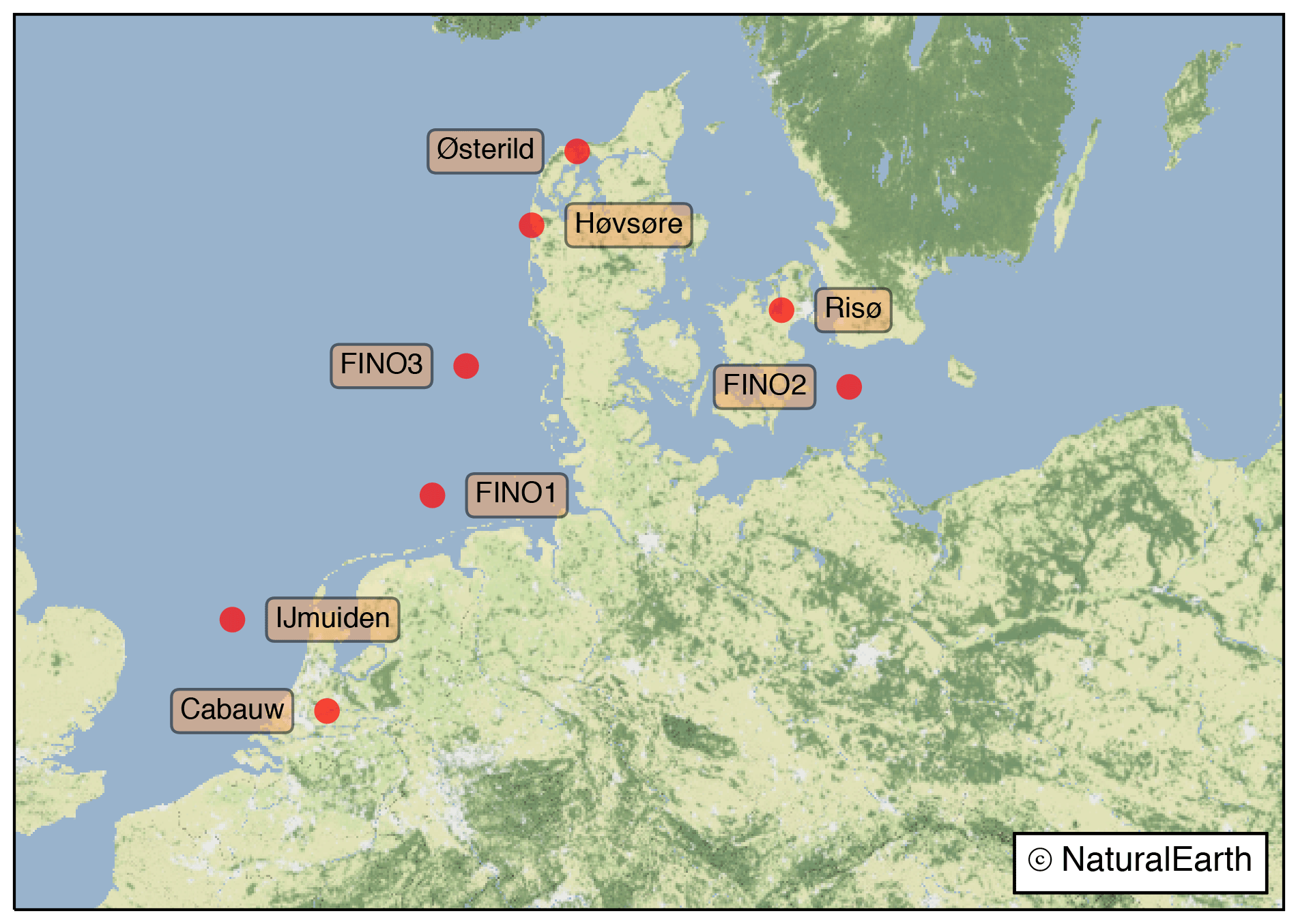
Figure 1 Location and name of the tall mast or lidar sites used in the model evaluation. Base map created with Natural Earth.

Table 1 Tall mast sites and wind measurement (WS: wind speed; WD: wind direction) heights available at each site. The values indicated in bold are used in the evaluation of wind profiles; the values underlined are those used in the evaluation of temporal variability. The centre of the sector where the mast can cause flow distortion and influence the wind speed is also listed. The last three columns show the data availability for 2015 for profiles, time series, and wind direction, respectively.

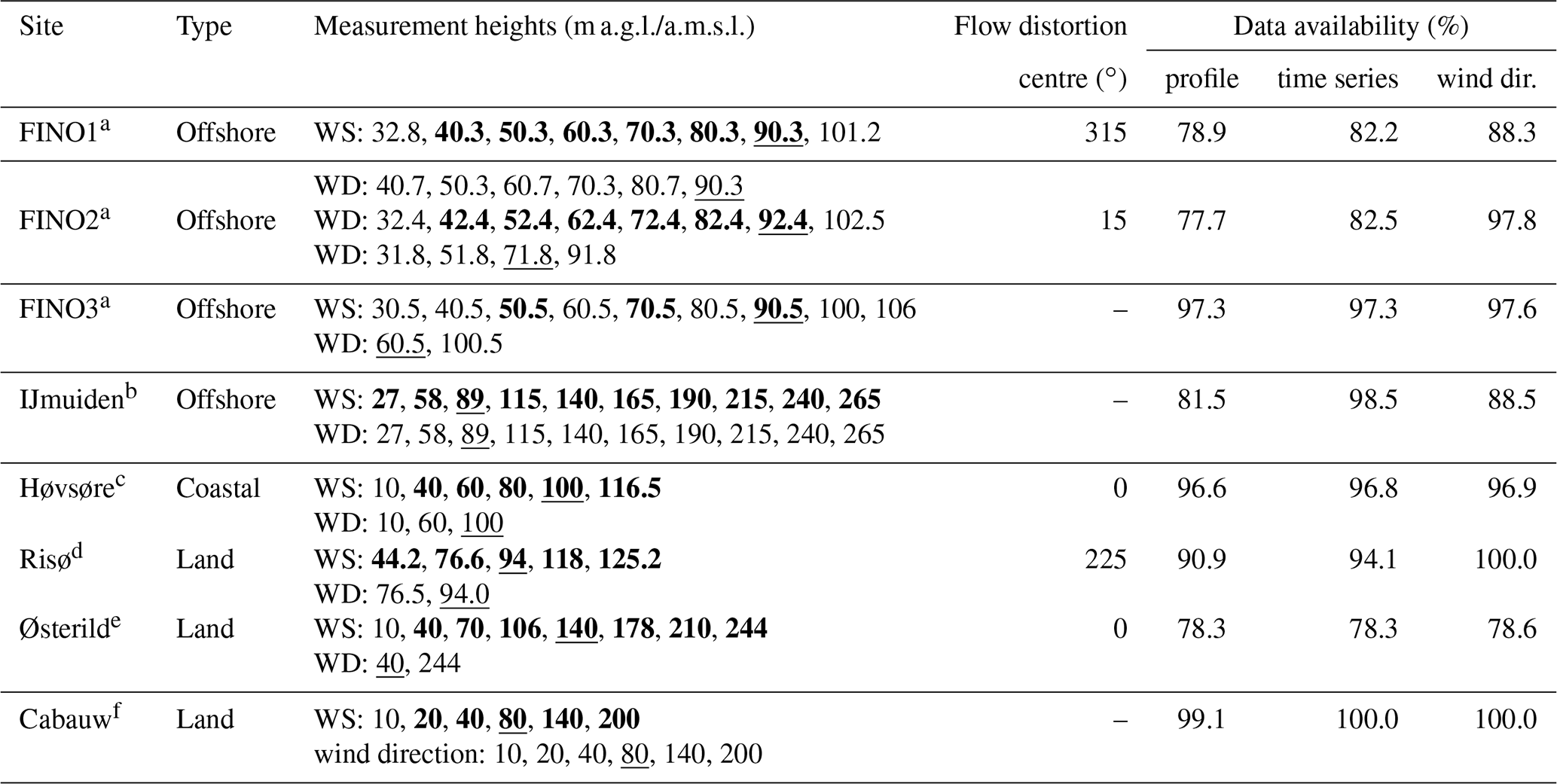
^a https://www.fino-offshore.de/en/ (last access: 18 October 2020). ^b Kalverla et al. (2017). ^c Peña et al. (2015). ^d http://rodeo.dtu.dk/rodeo/ProjectOverview.aspx?&Project=5&Rnd=674271 (last access: 18 October 2020). ^e Peña (2019). ^f http://www.cesar-database.nl (last access: 18 October 2020).

High-quality data are essential for model evaluation (Lucio-Eceiza et al., 2018a, b). The mast data have been quality controlled, and the mast flow distortion on the wind speed estimates was minimized by sub-setting the data. At FINO1, FINO2, Risø, and Høvsøre, where wind speed measurements are available from only one boom, winds originating from ±10^∘ of the boom direction are filtered. A misalignment correction to the wind direction was applied to the wind vanes at FINO1 (Westerhellweg et al., 2012). At FINO3, we use the data from the three heights where wind speed measurements from three booms are available. The wind speed value is taken from the boom where the wind direction is most perpendicular to the boom direction. At IJmuiden, the data were processed as discussed in Kalverla et al. (2017). At Cabauw, the data were processed and gap filled as described in Bosveld (2019).

In addition to mast flow distortion, the wind speed estimates at some of the measurement sites are impacted by nearby wind farms. At Høvsøre and Østerild, test turbines are located north of the mast, in the sector with the least frequent wind directions. At FINO1, the wind farm Alpha Ventus impacts the eastern sector, with the nearest turbine only 405 m away in the direction of 90^∘. The wind farm EnBW Baltic 2 started operation in September 2015 and lies directly to the southeast of the FINO2 mast. At FINO3, the DanTysk wind farm went into operation in December 2014 to the east of the mast. Due to the difficulty in understanding the impacts of the wind turbines on the measurements (e.g. times of operation at the onset can vary due to adjustments and testing), the data have not been filtered or corrected for the turbine wakes. However, the presence of the wind farm can impact the evaluation of the model results and should be kept in mind.

All measurement data are 10 min mean values. It was filtered to one period per hour, using the period that was closest to 00 min. The additional filtering for mast flow distortion process removes a small number of samples. For the time series evaluation, we used measurements from the level that was closest to 100 m a.m.s.l. (above mean sea level) and had a good data availability (underlined values, Table 1). The choice of the wind direction height for the model evaluation and data filtering uses the same procedure.

4 Model evaluation metrics

The main goal of the NEWA sensitivity study was the evaluation of the wind climate, which is usually understood as the probability distribution of wind speed and direction at a specific point. Thus, we used several metrics to evaluate the accuracy of the model simulations when compared to tall mast observations tailored to this purpose.

We calculate the temporal mean of each modelled distribution, ${\stackrel{\mathrm{‾}}{u}}_{\mathrm{m}}$, and the observed distribution, ${\stackrel{\mathrm{‾}}{u}}_{\mathrm{o}}$, for identical time periods. The bias herein is defined as difference between the two means, ${\stackrel{\mathrm{‾}}{u}}_{\mathrm{m}}$–${\stackrel{\mathrm{‾}}{u}}_{\mathrm{o}}$. If the bias is positive, the model overestimates the observed wind speed.

The bias is a popular error statistic for comparing the wind speed distributions between observations and model-simulated fields. However, the shape of the wind speed distribution is more important in wind energy applications because the wind power density is proportional to the cube of the wind speed. Thus, small changes in the wind speed distribution are amplified when converted to power. Accordingly, we introduce the Earth Mover's Distance to evaluate the differences in the shape of two frequency distribution. The Earth Mover's Distance (EMD), also known as the first Wasserstein distance, is popular in image processing (Rubner et al., 2000). The EMD can be interpreted as the amount of physical work needed to move a pile of soil in the shape of one distribution to that of another distribution. More discussion about the EMD properties can be found in Lupu et al. (2017). For one-dimensional distributions the EMD is equivalent to the area between two cumulative distribution functions, and this interpretation, with slight modifications, can also be applied to circular variables (Rabin et al., 2008). The EMD was calculated using the Pyemd package (Pele and Werman, 2008).

Figure 2 illustrates the differences between the EMD and the absolute value of the bias. Figure 2a shows the relationship between the EMD and the absolute value of bias for two WRF model simulations for all points in the domain. Figure 2b shows modelled wind speed distributions for two separate grid points. This highlights the case where two differently shaped distributions can have the same mean. The EMD helps clarify such occurrences. For one-dimensional distributions the EMD can be calculated as the area between the cumulative distribution curves, as illustrated in Fig. 2c.

Figure 2 (a) Relationship between EMD values and absolute value of bias between the wind speed in two WRF model setups for all grid points in the domain. The red dot represents an example where the EMD and the absolute value of bias are different. (b) Wind speed distributions of the two ensemble members corresponding to the red dot. (c) Cumulative probability distribution together with the EMD value calculated as the area between them. Distributions are the same as in (b).

The circular EMD (CEMD; Rabin et al., 2008) extends the EMD concept to one-dimensional circular histograms, such as the frequency distribution of wind directions. Two examples of the value of the CEMD are given in Fig. 3 for FINO3 and FINO1. At FINO3, the observed and simulated wind direction distributions are very similar and the value of CEMD is 2.18^∘, mainly due to differences in frequency within the same sector. A higher value of CEMD (=5.28^∘) is obtained when a rotation in the wind direction is found between the observed and simulated wind directions. The CEMD is used throughout the paper, and is to our knowledge the first time that it is used for evaluating wind directions in meteorology or climate science.

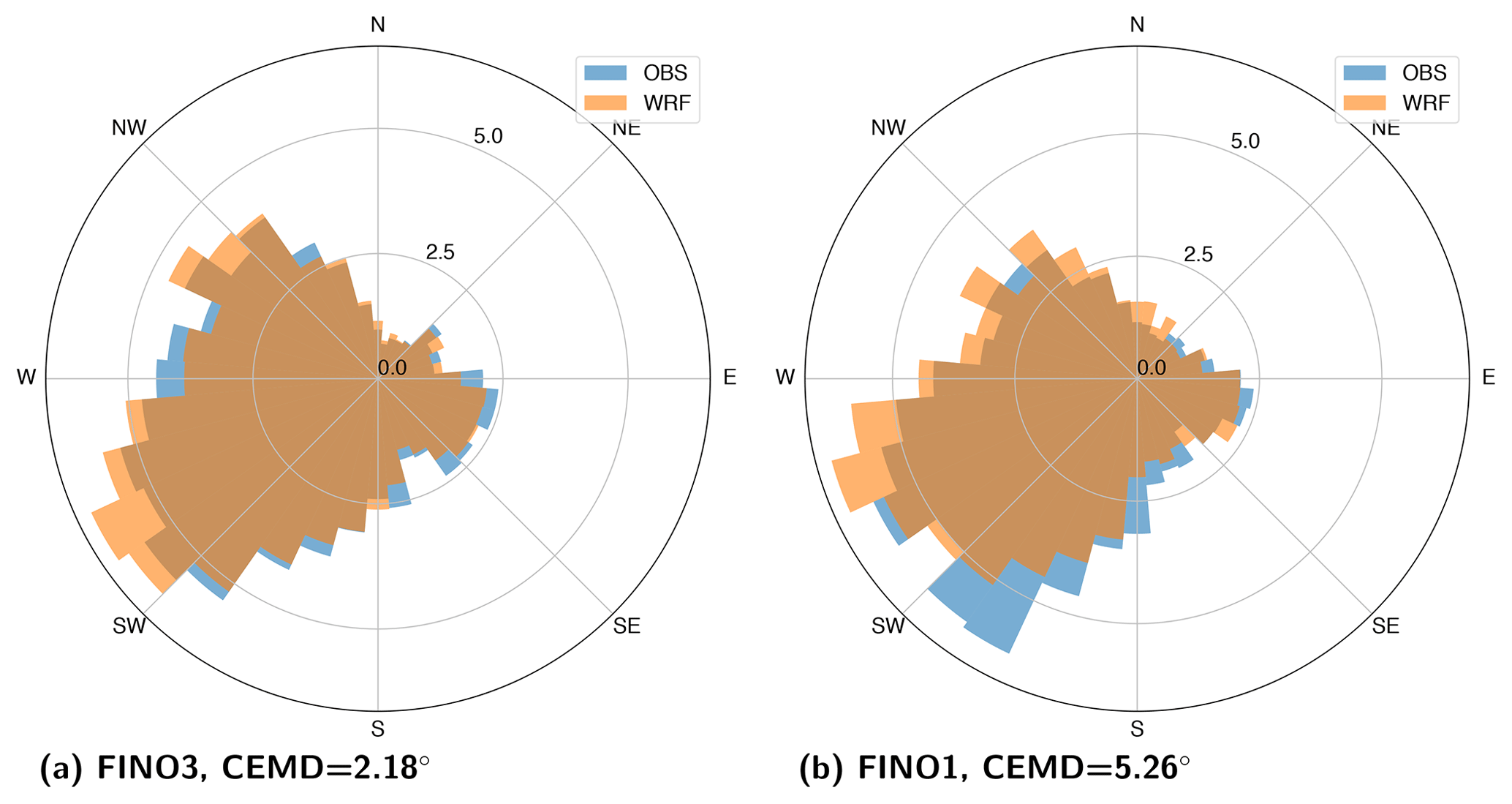
Figure 3 Wind direction distributions for (a) FINO3 and (b) FINO1, using measurements (OBS) and model-simulated (WRF) data.

The information about temporal co-variability is provided herein by root mean square error (RMSE), which estimates of systematic biases in model skill (von Storch and Zwiers, 1999). The RMSE is calculated over all i time steps:

$$\begin{array}{}\text{(1)}& \mathrm{RMSE}=\sqrt{{\displaystyle \frac{\mathrm{1}}{n}}\sum _{i=\mathrm{1}}^n{\left(u_{\mathrm{m}}^i-u_{\mathrm{o}}^i\right)}^{\mathrm{2}}},\end{array}$$

with $u_{\mathrm{m}}^i$ and $u_{\mathrm{o}}^i$ being the ith modelled and observed values in the time series of length n.

In this study, we compared a large ensemble of WRF model setups against the observations at several sites. One of the ensemble members was designated to be the baseline or “BASE”. The aim is to evaluate if a certain model setup from the pool performs better or worse than the baseline configuration. For this purpose we define a general skill score (von Storch and Zwiers, 1999):

$$\begin{array}{}\text{(2)}& \mathrm{SS}=\mathrm{1}-M_j/M_{\mathrm{B}},\end{array}$$

where M_j is the value of the metric for the jth ensemble member and M_B is that of the baseline. The metric M can be the absolute value of the bias, the RMSE, EMD, or CEMD. If SS>0 the ensemble member j “improves” the metric with respect to the baseline case and if SS<0 it “worsens” it. A value of SS=1 means that the new simulation is perfect. The SS is easily understood and is applicable to all our evaluation metrics. However, when the BASE simulation evaluates extremely well against observations (e.g. when the bias is close to zero), the skill score can become very large. Therefore, the SS is a useful quantity for the RMSE, which is rarely close to zero but can be misleading when used for the absolute bias or the EMD, indicating large improvements when the differences in metrics themselves are small. Accordingly, we suggest using both SS and the original metric when interpreting the results.

5 Sensitivity analysis of WRF simulations

In this section, the results from the different sensitivity experiments are presented and discussed. These are grouped into six subsections: Sect. 5.1 presents the results from five different domains for a small number of experiments to see how the results differ depending on the simulated region; Sect. 5.2 evaluates the results from one of these domains against observations; Sect. 5.3 highlights the impact of the WRF version on the wind speed results by investigating four different versions of the WRF model; Sect. 5.4 presents the results from a 25 simulation sensitivity study addressing the impact of the SL, PBL, and LSM schemes, including changes to the surface roughness length; Sect. 5.5 documents the impact of other parameterizations and forcing data; and finally Sect. 5.6 focuses on the impact of the size of the domain. It should be noted that these sections do not necessarily follow the chronological order that they were performed in the NEWA project but provide a logical progression of the decisions taken during the project.

5.1 Sensitivity to geographical domain

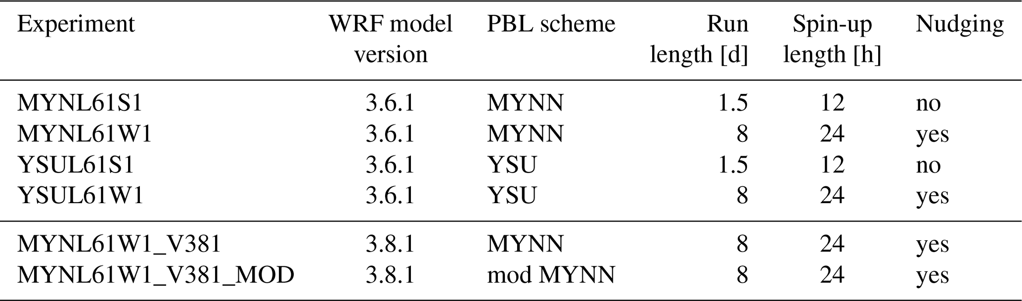
In the initial stage of the evaluation of the WRF model setup, we designed four numerical experiments (top four simulations in Table 2) over five different regions in Europe (Fig. 4), mostly located near countries represented in the NEWA team. The experiments explore the impact of using different PBL schemes, the MYNN (Mellor and Yamada, 1982) or the YSU (Hong et al., 2004), and the effect of different initialization strategies (short, S1, or weekly, W1, simulation length and excluding or including nudging). The YSU and MYNN schemes are non-local K mixing and TKE 1.5 order closure models, respectively. They were chosen because they are popular among the WRF model users and have shown good skill in previous studies (Draxl et al., 2014; Hahmann et al., 2015). The main objective was to clarify whether the sensitivity of the mean wind speed to these changes is similar in different geographic regions or there were regional differences. All other settings were fixed. The simulations were carried out with the WRF model version 3.6.1, released in August 2014. The basic WRF model setup includes using the ERA-Interim reanalysis (Dee et al., 2011) for initial and boundary conditions, NCEP optimal interpolation sea surface temperature (SST, Reynolds et al., 2007), and 61 vertical levels. Other details are given in Table A1.

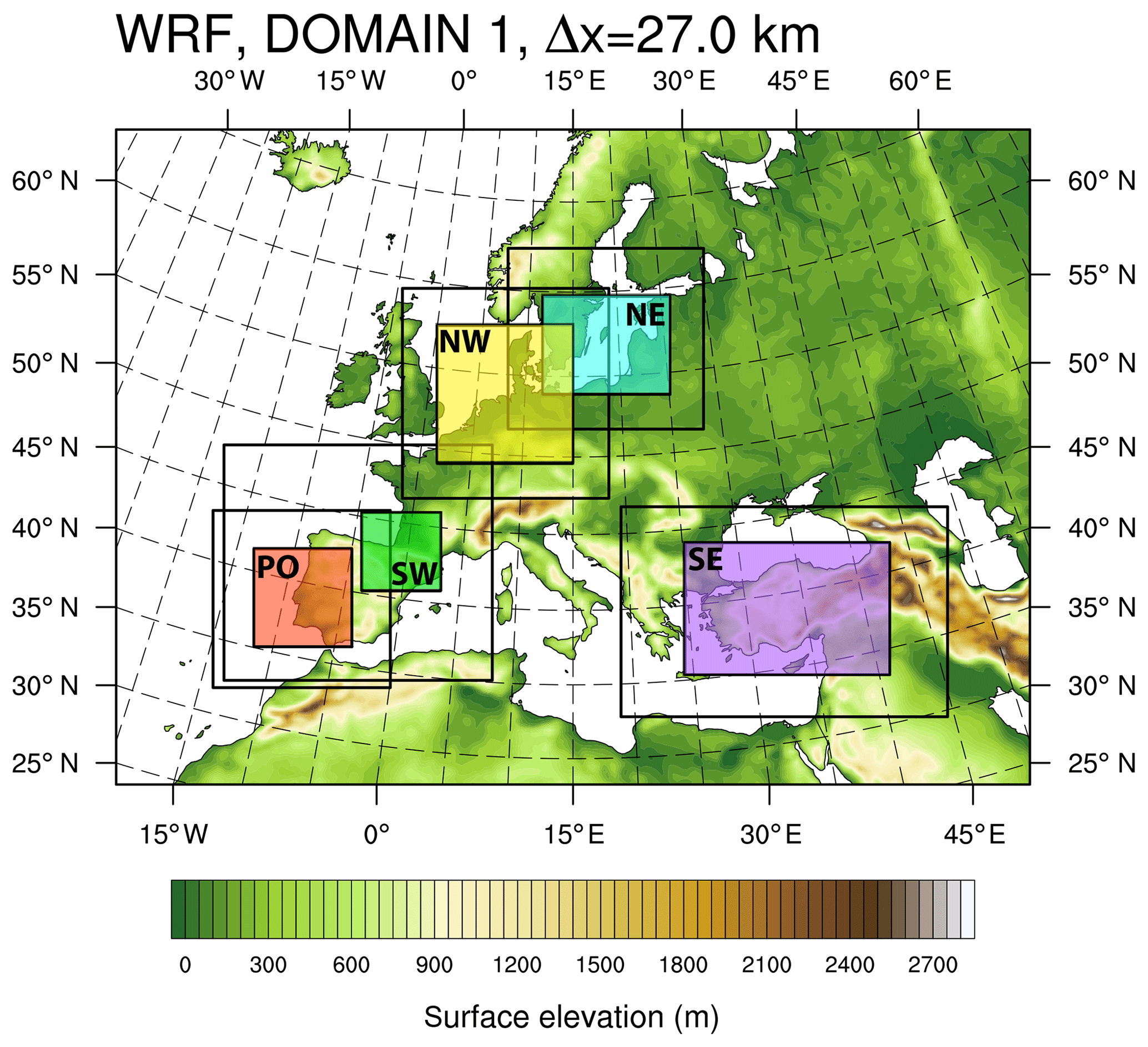
Figure 4 The location of the five inner domains (D3; NW, NE, SE, SW, and PO in coloured boxes) used in the geographic similarity experiments. The surface elevation of the WRF model outer domain (D1) is shown by colour; the black lines show the extent of D2. All inner domains share the same outer domain (D1), which corresponds to the area of the base map.

Table 2 Acronyms and relevant setup parameters of the WRF model sensitivity experiments oriented to address the influence of the geographic domain and WRF model version. The mod MYNN scheme is described in Sect. 5.3.

The analysis of the experiments presented in Fig. 5 show that on average the differences in annual mean wind are small and those that arise from the choice of PBL scheme are larger and more extensive than those from the initialization strategy. The largest differences in wind speed that arise from the initialization strategy (Fig. 5a and d) coincide with areas of elevated terrain in the western French Alps and the Pyrenees in the SW domain and the northwest corner of the NW domain. In these areas the daily runs (S1) have stronger winds on average than the weekly nudged simulations (W1). The largest differences in wind speed that arise from the choice of PBL scheme (Fig. 5b and e) coincide with the regions with particularly large surface roughness length, namely forests in southern Sweden and southwestern France. There, the experiment using the MYNN scheme provides wind speeds that are on average more than 0.5 m s⁻¹ lower than in the experiment using the YSU scheme. Over the sea, no significant difference is seen in the NW domain, and only slight differences (less than 0.3 m s⁻¹) exist above the Atlantic and Mediterranean (SW domain).

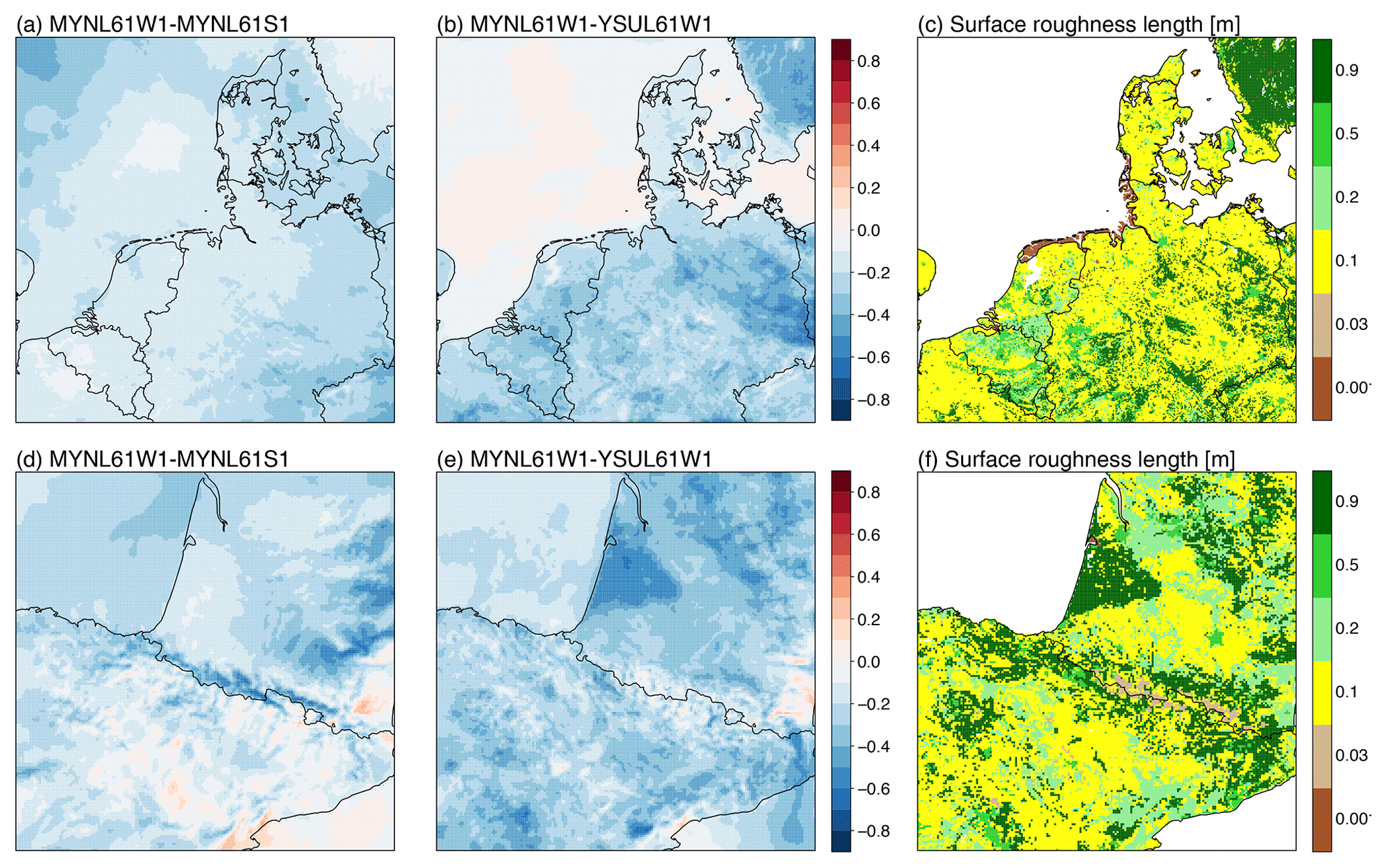
Figure 5 Annual mean difference in wind speed (m s⁻¹) between the simulations with different initialization strategies for the MYNN simulations (W1 minus S1; a and d), different PBL schemes (MYNN minus YSU; b and e), and surface roughness lengths (m) used in the simulations (c, f). Panels (a–c) are for the NW domain, and panels (d–f) are for the SW domain shown in Fig. 4.

Similar analysis was carried out for the other three domains in Fig. 4. All five domains show the same pattern of higher wind speed at 100 m for simulations using the YSU scheme over land, with the largest differences occurring over rougher terrain (e.g. forests). Over water, the differences are much smaller. The winds simulated using the YSU scheme are slightly higher than those simulated using the MYNN scheme but only in regions dominated by unstable stratification (e.g. the Atlantic Ocean, Mediterranean and Black Seas). In the nudged weekly simulations, wind speeds are overall reduced from those in the daily simulations, and to a higher magnitude over higher terrain and closer to the edge of the domain. Similar results were obtained in Hahmann et al. (2015) when the discarded spin-up time of the short simulations was varied. We hypothesize that as the model integration progresses, a balance is reached between the large-scale flow, the model physical parameterizations, and the surface forcing supplied by the terrain elevation and surface roughness. This process takes some time and results in lower wind speeds in the longer simulations. The effect is different on the northwest corner of the NW domain, which is the dominant inflow boundary, probably resulting from the nudging in the outer domain that is absent in the short runs. In summary, the effect on the wind speed when one of those PBL schemes is replaced with another is nearly insensitive to the location of the domain (i.e. north versus south).

Figure 6 Comparison of the observed mean wind speed (m s⁻¹) as a function of height for the eight sites and the simulated mean wind speed from the four sensitivity WRFV3.6.1 runs in Table 2.

5.2 Evaluation against observations in the NW domain

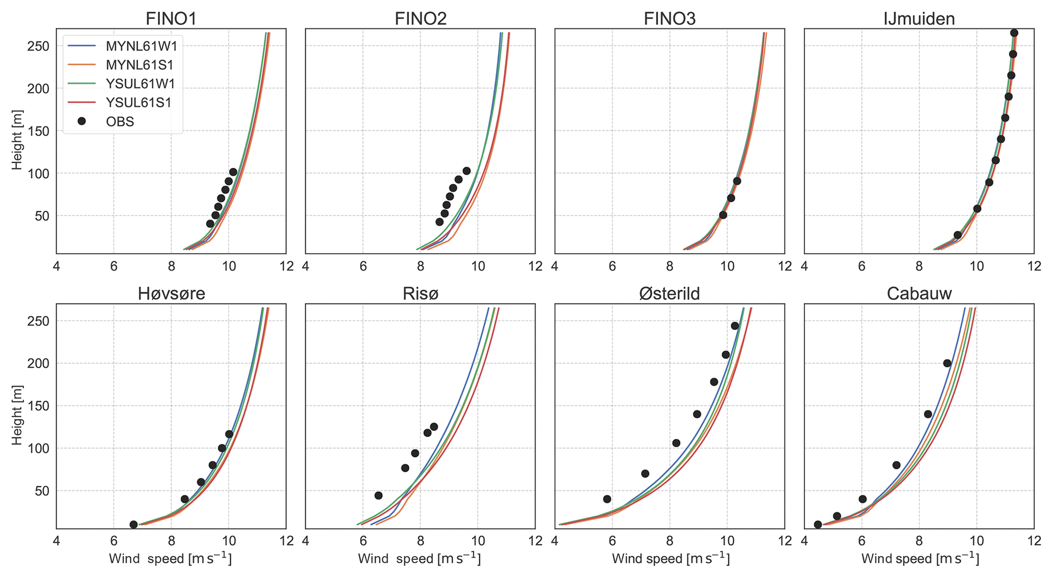
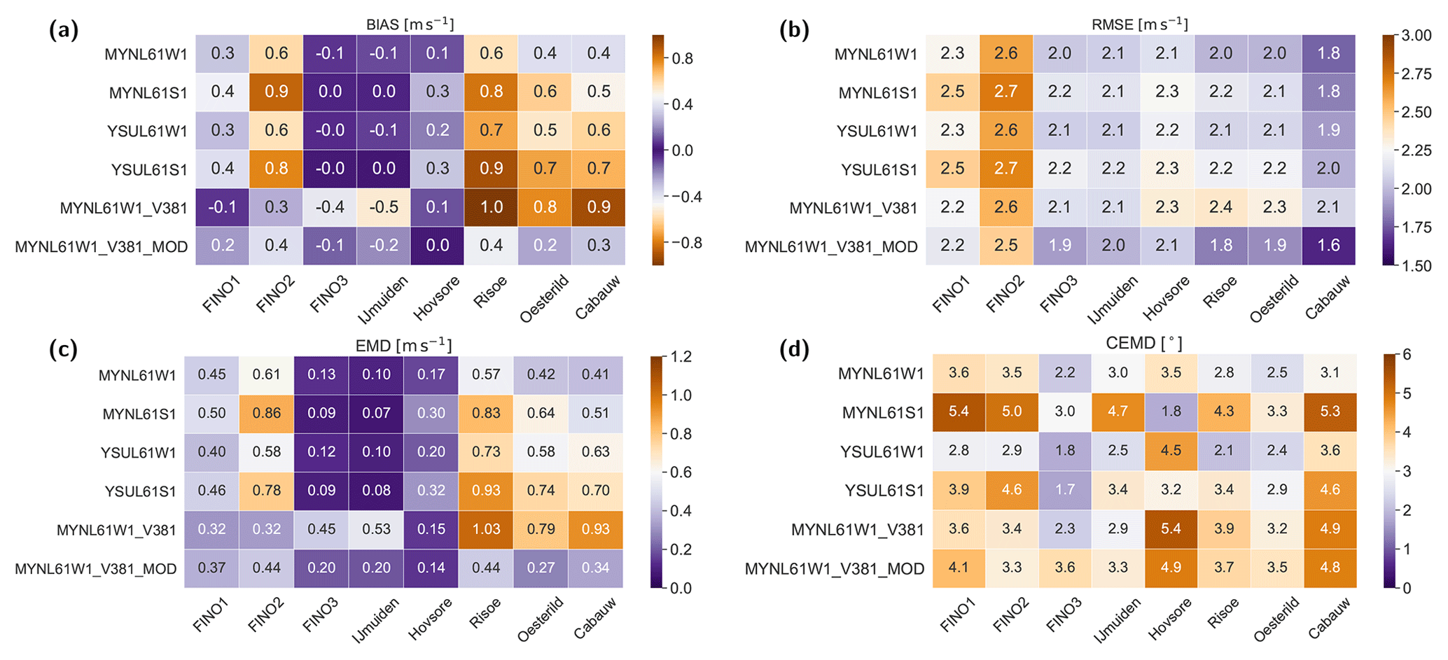
We evaluate the mean wind profiles from the four model setups in Sect. 5.1 to observations in the NW domain to proceed in determining a suitable model configuration. The evaluation of the mean wind speeds from the four WRFV3.6.1 sensitivity experiments against the mast measurements is shown in Figs. 6 and 7. The differences in mean wind speed between the various experiments are small. The mean wind profile from the MYNL61W1 simulation is closest to the observed profile at nearly all the sites, except at the offshore sites where the MYNL61W1 and YSUL61W1 are nearly indistinguishable from each other. The evaluation metrics of the wind speed and direction for the experiments and sites are presented in Fig. 7. This confirms that the wind speeds from the MYNL61W1 simulation have the lowest biases at Cabauw, Høvsøre, Østerild, and Risø and the lowest RMSE at all sites, except for FINO1 and IJmuiden, where the results from MYNL61W1 and YSUL61W1 are virtually the same. The EMD shows the lowest values for the weekly nudged simulations compared to the short runs, and for the coastal and land sites the lowest EMD is for the MYNL61W1 simulation. Similar conclusions apply to the CEMD of the wind direction, where the YSUL61W1 performs the best at six of the eight sites.

Figure 7 Evaluation metrics, i.e., (a) bias (m s⁻¹), (b) RMSE (m s⁻¹), (c) EMD (m s⁻¹) for the simulated wind speed and (d) CEMD (^∘) for simulated wind direction, at the eight sites and underlined heights in Table 1 and the sensitivity experiments in Table 2.

In summary, the weekly nudged simulations for both MYNN and YSU schemes result in lower biases and lower RMSE at all sites. Because the effect on the wind speed when one of those PBL schemes is replaced with another is nearly insensitive to the location of the domain (i.e. north versus south) as shown in Sect. 5.1, we continue under the assumption that it is valid for other regions in Europe, except for regions with more complex terrain, which have not been evaluated. The weekly nudged simulation setup was chosen for the remainder of the NEWA sensitivity simulations. The setup and constants used in the nudging will be re-evaluated in the sensitivity experiments in Sect. 5.5.

5.3 Sensitivity to properties of the MYNN scheme

We also tested the version of the WRF model used during the sensitivity analysis to evaluate whether changing the version implied any difference with respect to the baseline configuration described above. At the time of the development of this work, the latest version was WRF version 3.9.1, released in August 2017. The simulations using versions WRFV3.8.1 and WRFV3.9.1 use the same NW domain and the same model setup as in the MYNL61W1 simulations (Table 2). The results for WRFV3.6.1 and WRFV3.8.1 are presented in Figs. 7 and 8; the results for WRFV3.9.1 (not shown) are nearly identical to those from WRFV3.8.1.

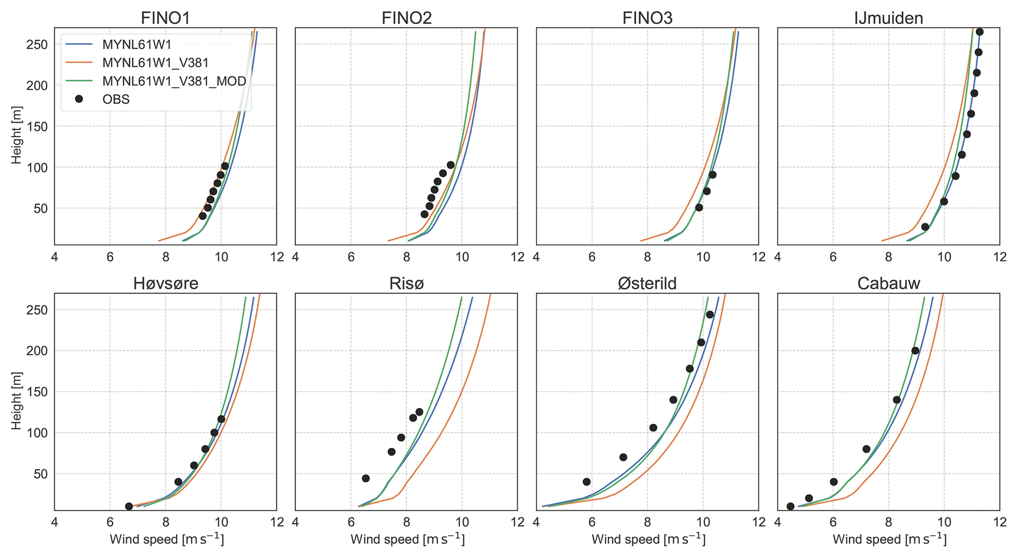
Figure 8 Comparison of the mean observed wind speed (m s⁻¹) as a function of height for the eight sites and the mean wind speed in the simulations using WRFV3.6.1, WRFV3.8.1, and the modified version of WRFV3.8.1_MOD described in Table 2.

The wind speed from simulations using WRFV3.8.1 presented an increased bias compared to observations for all sites and most levels, except for FINO1 and FINO2, which suffer from flow distortion and wind farm effects. The increased bias was traced back to changes in two important equations in the MYNN SL and PBL scheme, which became defaults in WRF version 3.7. The first is the scalar roughness length over water, which was changed from the formulation in Fairall et al. (2003) to that in Edson et al. (2013), thus affecting the wind speed over the ocean. The second is a change in the definition of the mixing length (Olson et al., 2016). Both of these options could be customized and set as in the baseline configuration. Results from such a setup are labelled “WRFV3.8.1_MOD” in Fig. 8. Some of the previous characteristics of the profile are restored after these changes, and the simulation using WRFV3.8.1 with modifications improved the RMSE and EMD for all sites (Fig. 7. These changes are consistent with those found by Yang et al. (2017) for the MYNN scheme. Although above ∼100 m the simulation using the modified WRFV3.8.1 gives lower mean wind speeds than WRFV3.6.1 at all sites, we nonetheless consider that this difference is less relevant, and based on the improvements of the scheme “WRFV3.8.1_MOD”, this setup was selected as the baseline, named “BASE” from hereon. The WRF model setup of this baseline is summarized in Table A1. Unless explicitly labelled otherwise, when referring to the MYNN option in the remainder of this work we mean the modified version of the scheme. The unmodified MYNN PBL will be referred to as MYNN^*.

5.4 Effect of surface and planetary boundary layer and land surface model

Having set our baseline configuration, we now start testing other possible modifications to the model setup and parameterization options. The first series of sensitivity studies tested the sensitivity of the near-surface wind to various combinations of LSM, PBL, and SL schemes and the specification of surface roughness length. The combinations tested are listed in Table 3. All the simulations listed here and most of those in Sect. 5.5 use the ERA5 reanalysis (Hersbach et al., 2020) as the source of initial and boundary conditions.

Table 3 Overview of the ensemble of WRF model simulations' varying LSM, PBL, and SL schemes and the vegetation lookup table carried out for the NW domain. The names of the schemes are as follows: LSM: NOAH (Tewari et al., 2004), RUC (Benjamin et al., 2004), PX (Noilhan and Planton, 1989), SLAB (Dudhia, 1996), and NOAH-MP (Niu et al., 2011); PBL and SL: YSU (Hong et al., 2006), MYJ (Mellor and Yamada, 1982), MYNN (Nakanishi and Niino, 2006), modified MYNN (see Sect. 5.3), ACM2 (Pleim, 2007), MM5 (Jiménez et al., 2012), and M-O surface layer (Janjic and Zavisa, 1994). The number in parenthesis is the respective namelist value in the WRF model configuration file. The “simulation code” is explained in Appendix A2.

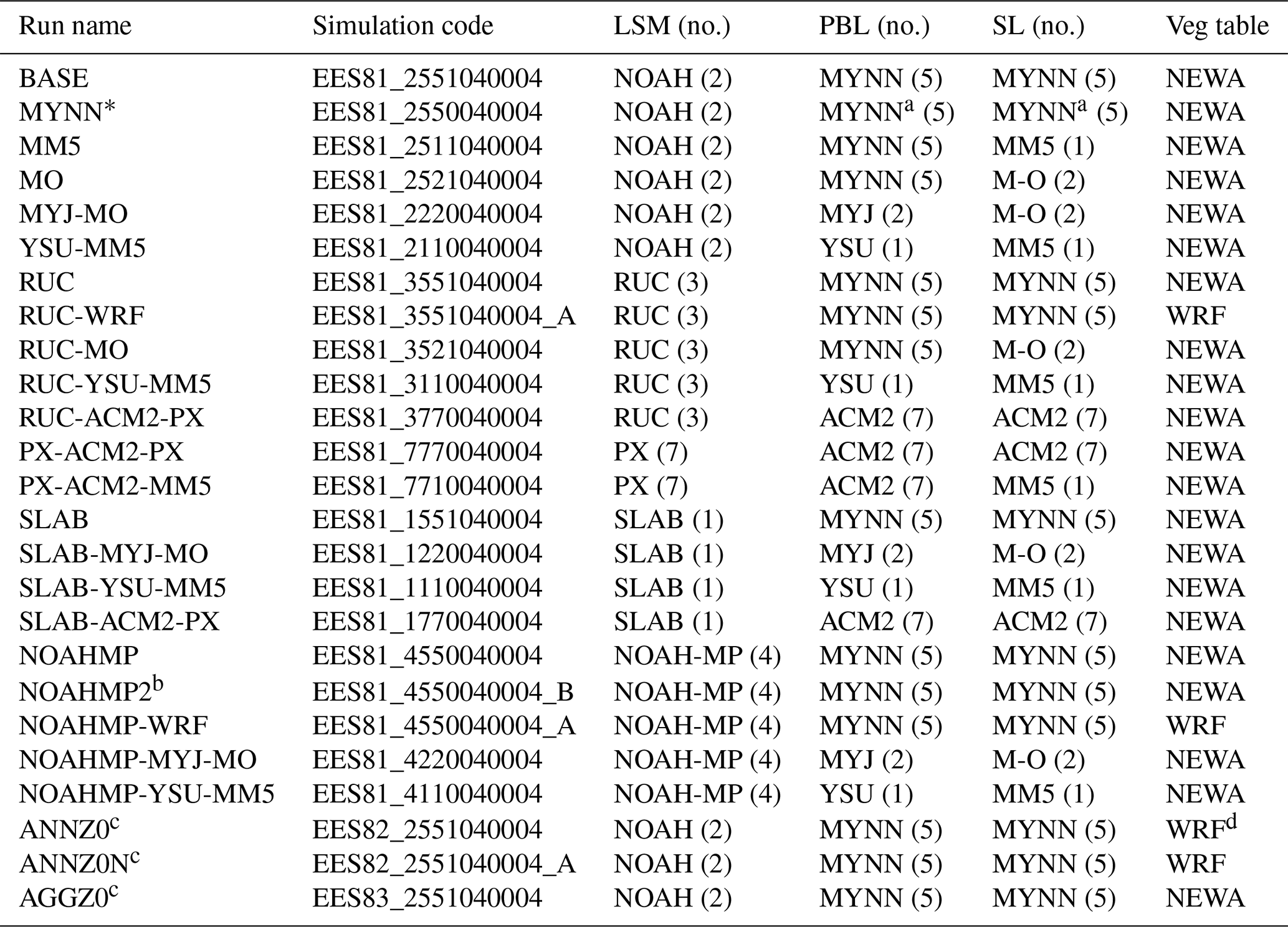
^a The unmodified MYNN scheme. ^b Using opt_sfc = 2 in the NOAH-MP scheme. ^c Differing in surface roughness; see text for details. ^d WRF table, but with low roughness for tidal zone.

The large number of schemes and their potential combinations led to a large number of possible combinations. In this work a total of 25 different combinations were tested, listed in Table 3, including changes in parameters in the schemes themselves. We also included the simulation using the MYNN^* scheme. Our original table of sensitivity experiments contained many other LSM–PBL–SL combinations, but some of these suffered from diverse technical issues and did not complete the runs. In some cases, small adjustments were needed. For example, in the experiments using the MM5 or MO surface layer schemes the fractional sea ice option had to be turned off.

An important aspect of the LSM, PBL, and SL sensitivity studies was the use of an alternative lookup table for the surface roughness length as a function of land use class. A custom NEWA lookup table was created since many values used in the WRF-distributed tables do not match the aerodynamic characteristics of European vegetation, especially over forests (Hahmann et al., 2015; Floors et al., 2018a). The new lookup table was created by polling wind energy resource assessment experts from the NEWA consortium. Both the new and old values of surface roughness length for each roughness class are shown in Table 4. Some of the larger changes include “Herbaceous Wetland”, which has an original value of z₀=0.20 m, but in the NEWA region represents the tidal zone in coastal Holland, Germany, and Denmark that is much smoother (Wohlfart et al., 2018) and thus was changed to z₀=0.001 m. The forest classes were also significantly changed, with the z₀=0.50 m value in the default table being changed to z₀=0.90 m, which is more representative of forests in, for example, Sweden (Dellwik et al., 2014) . The new roughness values should be considered only as estimates and as such there might be some limitations in the representation of the roughness length, they are nevertheless much more realistic than the default ones. The experiments using the standard vegetation tables are labelled WRF vegetation in Table 3.

Table 4 Vegetation lookup table for the surface roughness length as a function of the USGS land use category (Anderson et al., 1976) in the NEWA and default NCAR WRF model configuration. Only values changed from default are shown.

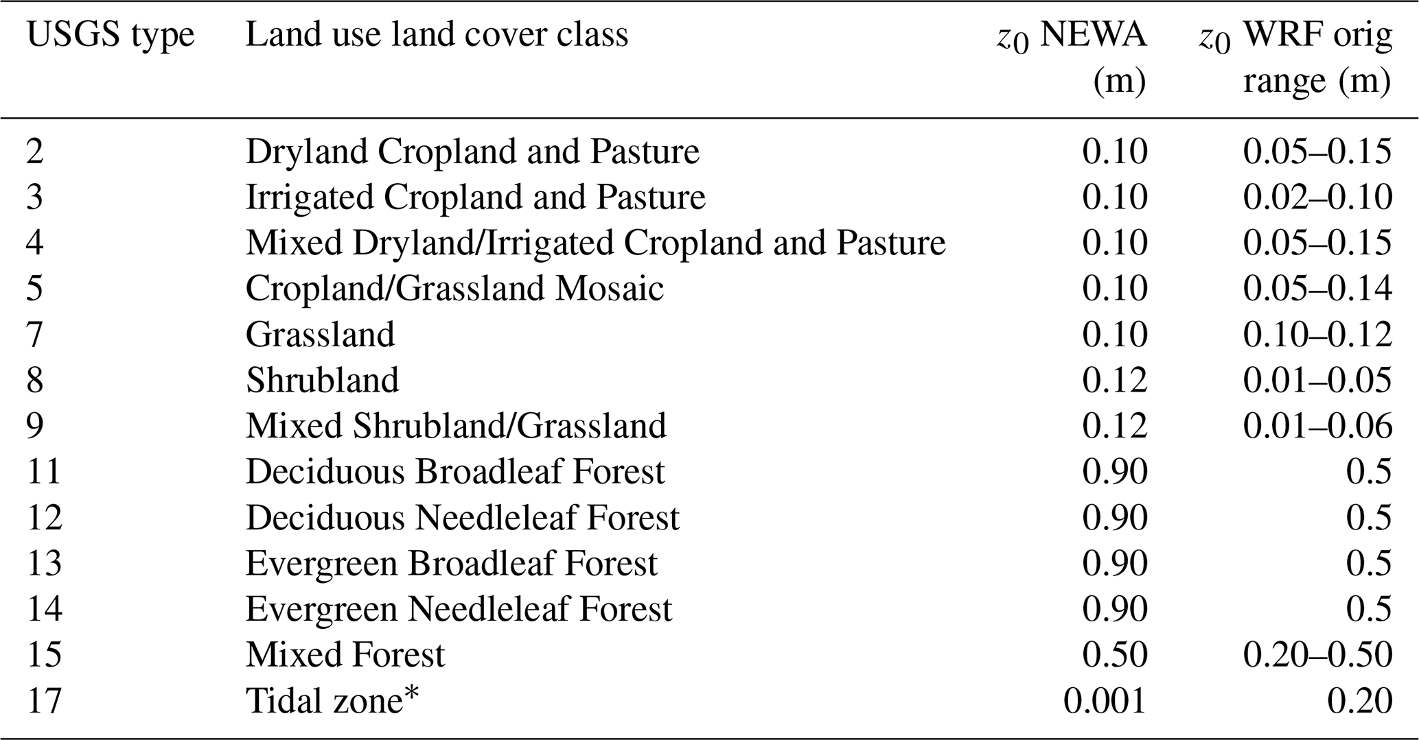
^* Originally called “Herbaceous Wetland” in the default WRF model vegetation table.

All NEWA setups use a constant value of surface roughness and have no annual cycle, except for two of the setups (ANNZ0 and ANNZ0N) that have annual cycle according to the default WRF vegetation table (except for the tidal zone). In WRF, the seasonality of the surface roughness length is controlled by the value of the green vegetation fraction (Refslund et al., 2014) and applies mostly for cropland classes in Table 4. The annual cycle of green vegetation fraction does not change from year to year and is spatially inconsistent with the ESA-CCI land use dataset used in the NEWA simulations. Therefore, because of inherent uncertainties, in NEWA we have chosen to use a single constant value of roughness for land use and land cover class. Also, since the WRF wind climatologies will be further downscaled, as described in Dörenkämper et al. (2020), using a constant value of surface roughness facilitates the process. Another roughness-related experiment that was included, AGGZ0, uses the sub-tiling option for NOAH (Li et al., 2013), with the NEWA vegetation table. The sub-tiling option generates more realistic values of surface roughness length in areas of mixed vegetation, which could reduce the biases in wind speed (Santos-Alamillos et al., 2015).

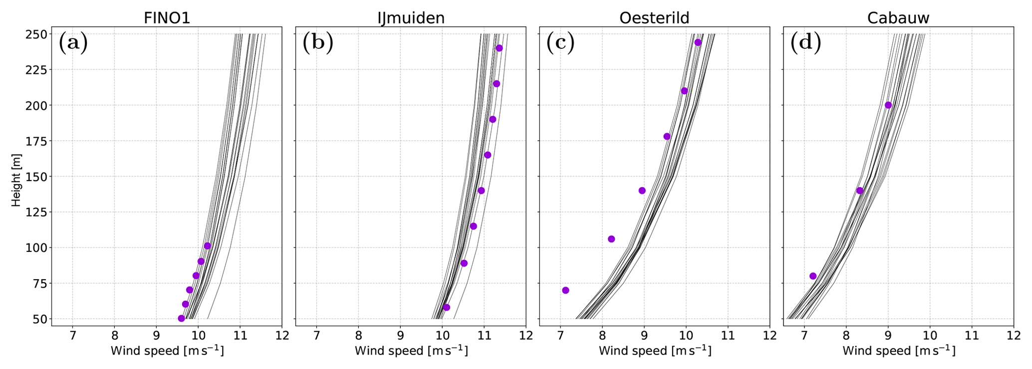
Figure 9 Mean wind speed (m s⁻¹) simulated by the various experiments in the LSM–SL–PBL ensemble as a function of height for four sites: (a) FINO1, (b) IJmuiden, (c) Østerild and (d) Cabauw. The observed values are shown as purple dots.

The vertical profiles of mean wind speed for all the LSM, PBL, and SL sensitivity experiments for four of the eight evaluation sites are shown in Fig. 9 as an example. The spread in the wind speed among the simulations excluding outliers generally increases with height, reaching around 1 m s⁻¹ at 100 m. Over land, for example at Østerild, the observed wind speed profile below ∼150 m lies well below the simulated values for all experiments, signifying a lack of representativeness of the surface conditions in the WRF model at this site, since the biases are independent of the LSM, PBL, or SL used.

To facilitate the intercomparison among the ensemble members, we computed all the evaluation metrics of the wind speed and direction for each simulation (Fig. 10). The metrics compare the filtered wind speed observations and wind directions during 2015 at the levels underlined in Table 1 with the corresponding WRF-simulated time series interpolated to the same height. Figure 10a shows the model bias at all the sites. For this metric differences among stations are larger than differences between models in a single station, expressed in this figure as consistent colours for each column. On average the characteristic of the bias relates most directly to the quality of the measurements and type of site, i.e. a slightly negative bias over the sea and a positive bias over land. The latter is likely a consequence of deficient representation of the land characteristics around each site. Some other general patterns are that the simulations using the MYJ scheme tend to have largest absolute biases, except at FINO3, and that the YSU-MM5-RUC simulation is an outlier, whose results differ from other setups, typically being among the worst of setups for any station.

To better quantify the differences between the simulations, Fig. 10b shows the skill score (SS) of the bias from the BASE simulation as defined in Sect. 4. Positive numbers (in purple) show a decrease in absolute bias, which point to a more accurate simulation. From these values some conclusions can be drawn. First, the differences between the simulations are quite modest: a maximum SS of 0.9 in the MM5 and MYJ-MO simulation at FINO1 and FINO3 and large values (up to $\mathrm{SS}=-\mathrm{16.2}$) in several simulations at Høvsøre. These large negative SS are an artefact of the very low bias in the BASE simulation at this site. Second, no simulation is capable of improving or degrading the bias at all of the sites: the SLAB simulation improves the bias (i.e. SS>0) at three of the eight sites, while the MO simulation improves the bias at five of the eight sites. The MYNN^* scheme considerably degrades the simulations at seven of the eight sites. The latter supports our decision to use the modified version of the MYNN scheme as a baseline. It is relevant to note that the changes in z₀ only cause minor variations in the biases (see members ANNZ0, ANNZ0n, AGGZ0); however, the sites are located in regions with vegetation classes that were not changed significantly from the WRF model standard table (Table 4).

Figure 10c and d provide further information about the sensitivity tests based on the EMD metric defined in Sect. 4 to evaluate the shape of the wind speed distributions. As with the bias, the EMD shows that the largest differences in total error are linked to the site location, with the best model performance at Høvsøre with EMD between 0.1–0.4 m s⁻¹, while at Risø the results fall between 0.4–1.0 m s⁻¹. Particularly interesting is the comparison between bias and EMD, since for most setups and stations the values of EMD and bias are similar, especially when the model results are significantly different from the observations. The EMD allows us to identify cases where the change in model setup improves only the mean value of distribution, as opposed to the similarities of the whole distribution. For instance, if only the biases were analysed, it could be argued that MYJ-MO is better than the BASE in FINO3 and IJmuiden, while the EMD show that there is only a modest improvement over the BASE at IJmuiden and a worse result at FINO3. Similar conclusions can be drawn for the SLAB-MYJ-MO and YSU-MM5-RUC simulations. As with the bias, no simulation improves the EMD for all sites, and very few simulations improve the EMD at all, especially for the land sites. The SLAB simulation improves the EMD at four sites (SS>0.1), while the MO simulation improves the EMD at three of the eight sites.

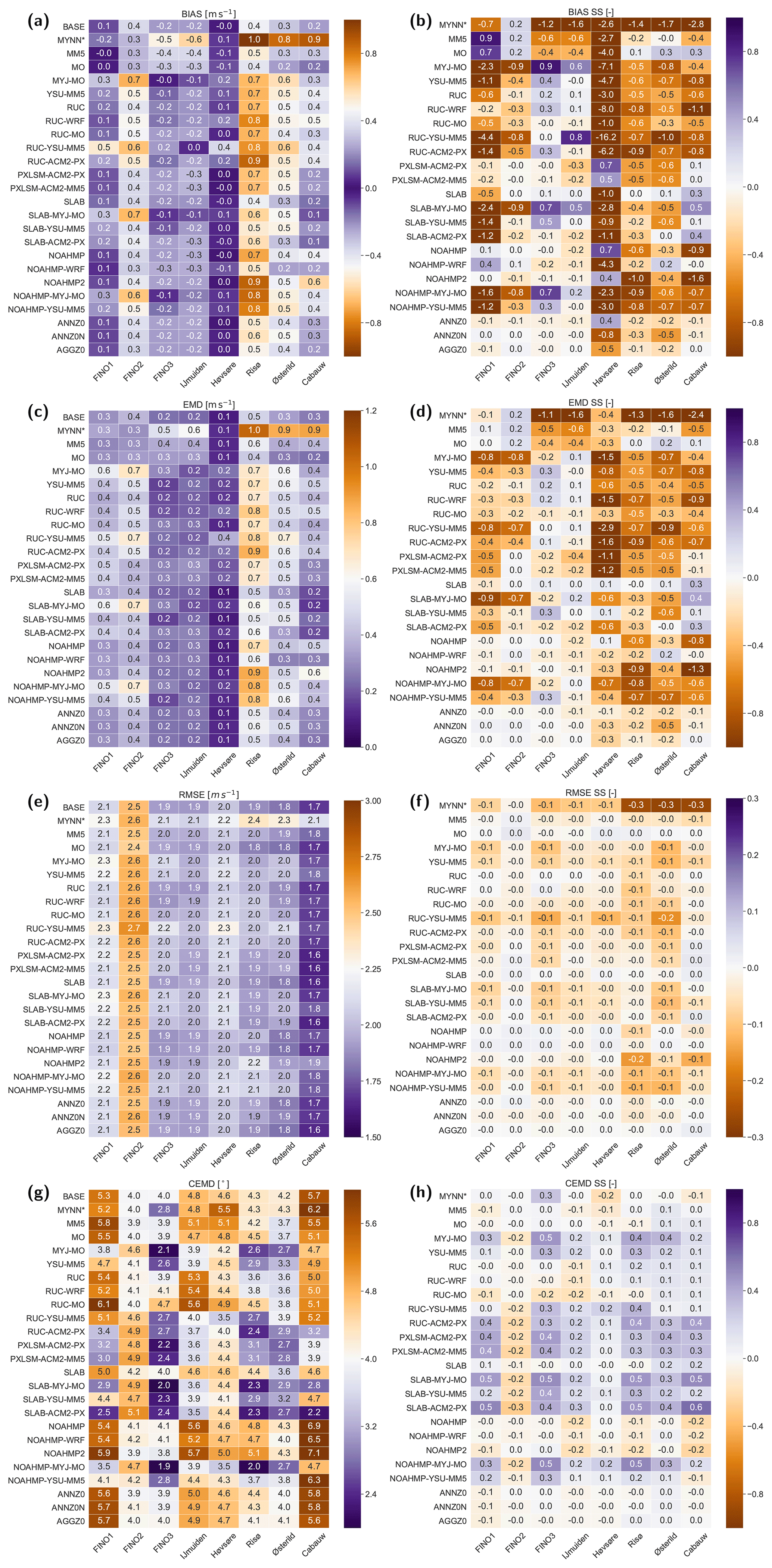
Figure 10 Evaluation metrics, i.e. (a) bias (m s⁻¹), (b) bias SS (–), (c) EMD (m s⁻¹), (d) EMD SS (–), (e) RMSE (m s⁻¹), (f) RMSE SS (–), (g) CEMD (^∘), and (h) CEMD SS (–), between the observed and simulated wind speed and wind direction at the eight sites and underlined heights in Table 1 and the various sensitivity studies in the LSM–SL–PBL ensemble (Table 3). All SS are relative to the BASE simulation.

Two other metrics are presented in Fig. 10: the RMSE for the wind speed (Fig. 10e) and the circular EMD (CEMD) for the wind direction (Fig. 10g) and their respective SS from the BASE simulation (Fig. 10f and h). As with the bias and EMD, the RMSE is primarily site dependent, with small differences between the simulations. The RMSE is lowest at Cabauw (1.6–2.1 m s⁻¹) and highest at FINO2 (2.4–2.7 m s⁻¹). No simulation significantly improves the RMSE, but it remains unchanged at all sites in the MO, SLAB, NOAHMP-WRF, and the all the varied roughness ensembles. The CEMD of the wind direction is variable among sites and simulations, but all the values are small (1.9–7.1^∘). For this metric, the MO and SLAB show similar values to the BASE simulation.

5.5 Other sensitivity experiments

A second set of sensitivity experiments was carried out to identify other factors that could potentially be important for the simulation of wind speed and direction within the WRF model. These experiments are listed in Table 5 and can be grouped into three main categories. First, we tested the impact of various initial and boundary conditions by using ERA-Interim, MERRA2, and FNL fields as forcing. The effect of various sources of sea surface temperature (SST) was also tested. In a second set, we tested other model dynamics, including the effect of spectral versus grid nudging, enlarging the lateral boundary zone, changing the wavelength of the minimum spectral nudging length, and enabling two-way nesting. The third set of experiments tested other model physics not related to the surface and PBL, i.e. radiation, cumulus convection, and explicit moisture schemes.

(Dee et al., 2011)(Gelaro et al., 2017)(NCAR, 2000)(Gemmill et al., 2007)(Reynolds et al., 2010)(Collins et al., 2004)(Grell and Freitas, 2014)(Thompson et al., 2012)

Table 5 Overview of other sensitivity experiments carried out. The meaning of the simulation code is explained in Table A2 in the Appendix.

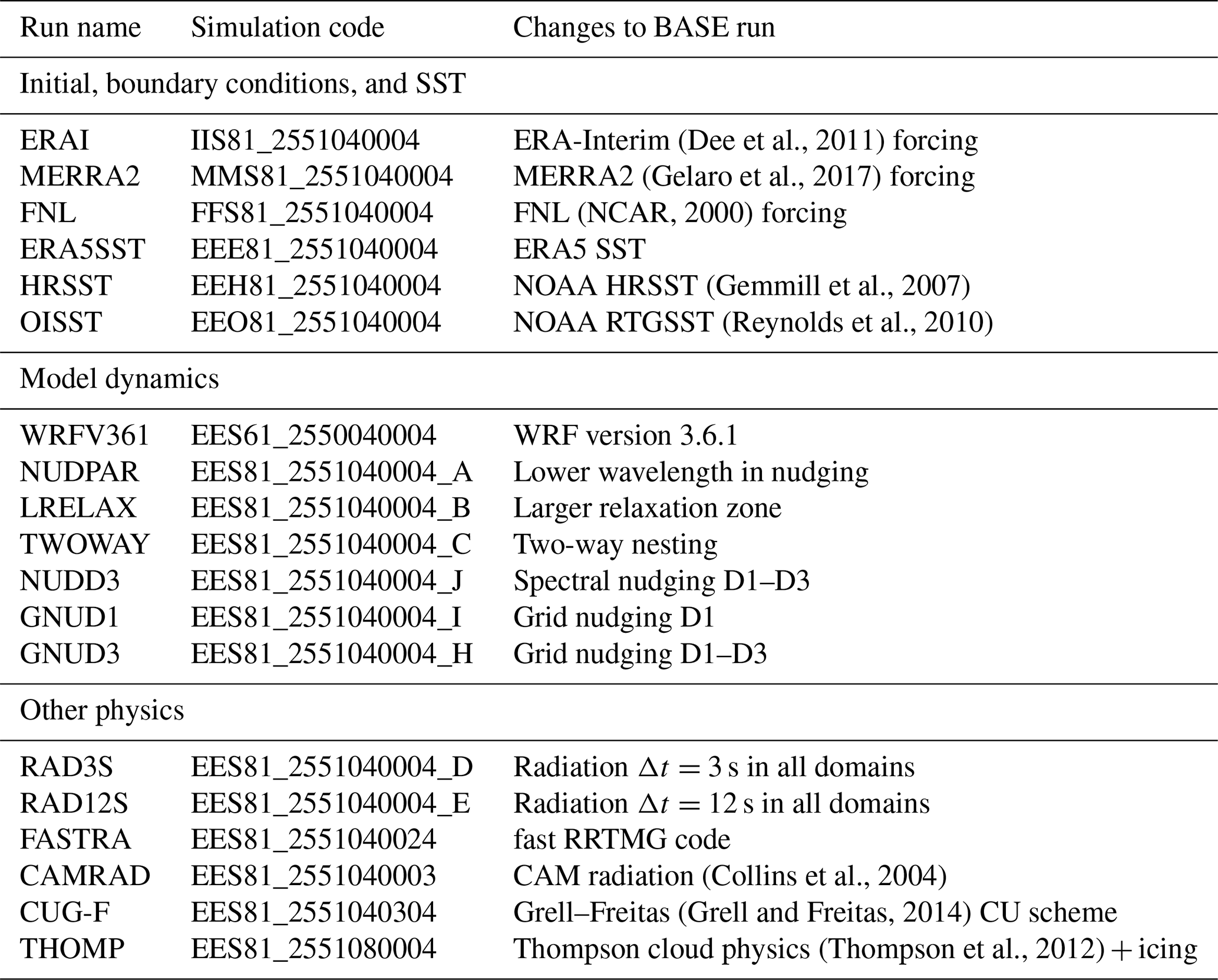
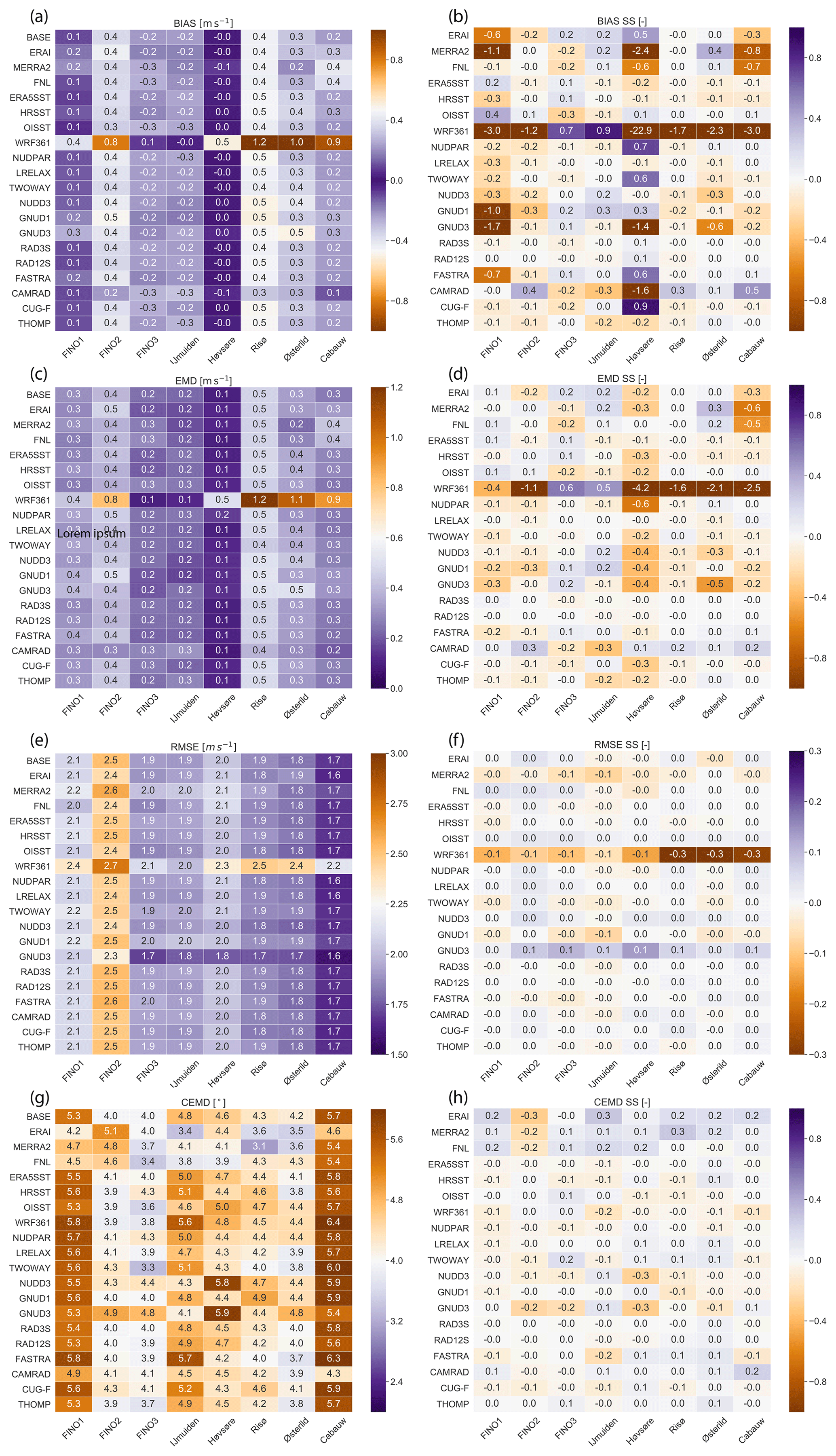
Figure 11 Evaluation metrics, i.e. (a) bias (m s⁻¹), (b) bias SS (–), (c) EMD (m s⁻¹), (d) EMD SS (–), (e) RMSE (m s⁻¹), (f) RMSE SS (–), (g) CEMD (^∘), and (h) CEMD SS (–), between the observed and simulated wind speed at the eight sites and underlined heights in Table 1 and the various sensitivity studies in the other ensemble (Table 5). All SS are relative to the BASE simulation.

Figure  shows all the evaluation metrics of the wind speed and wind direction for each simulation for the other set of sensitivity experiments. In contrast to the LSM, PBL, and SL ensemble members, for the bias (Fig. a) these simulations provide results that are very similar to the BASE simulation, except for the WRF361, GNUD3, and CAMRAD simulations. Switching the source of initial and boundary conditions to ERA-Interim, MERRA2, or FNL has very small impact to the bias. Changing the source of SST has negligible effect for all of the offshore masts. Most of the changes to the dynamic settings have very small consequences on the bias. The only larger change is the use of grid nudging in all three WRF domains, i.e. simulation GNUD3. The biases increase (SS≥0.1) in seven of the eight sites when this setting is activated; this is probably because of the slow down of the winds in the ERA5 reanalysis over land (see Fig. 9 of Dörenkämper et al., 2020). Interestingly, using this setting decreases the RMSE between the simulated and observed time series (Fig. f). Since the intent of the NEWA atlas is to provide an accurate description of the wind climatology, distribution metrics (e.g. EMD) are considered more important than time-dependent ones (e.g. RMSE).

The EMD and EMD SS for this set of sensitivity experiments was calculated and the results are shown in Fig. c and d. The conclusions about the usefulness of the EMD apply here as well. For instance, at FINO1 the ERAI and MERRA2 runs show an increase in bias compared to the BASE, while the EMD values show that these runs actually have more similar wind speed distribution to observations than the BASE. Otherwise, the EMD metric confirms the conclusions described earlier about the small impact of all of these changes and the relative decrease in quality when using grid-nudging (GNUD3).

Other dynamical and physics options, such as the radiation time step (RAD3S or RAD12S), the change of nudging constants (NUDPAR, LRELAX), or nesting (TWOWAY), show very small influence on nearly all the evaluation metrics. As with the LSM–PBL–SL, the simulations show very small differences in RMSE and CEMD with respect to the BASE, except for GNUD3 as mentioned above, which shows improved RMSE. It is also interesting to note that the ERAI, MERRA2 and FNL simulations show small improvements in the CEMD at many sites compared to the BASE simulation. The reason for this behaviour is not well understood.

In conclusion, many other changes to the WRF model settings have inconsequential effects to the simulation of the wind speed and direction at wind turbine hub height. The use of grid nudging in all domains (simulation GNUD3) improves the RMSE at most sites but has a negative effect to the BIAS, EMD, and CEMD. The change in radiation parameterization has a small effect in relation to the BASE simulation. Because the effect is small and the CAM radiation parameterization (Collins et al., 2004) is more expensive in terms of computational resources, it was ultimately not used in the NEWA production run.

5.6 Sensitivity to domain size

An additional decision to be made regarding the NEWA mesoscale simulations was the domain configuration, i.e. using a single large domain or several small domains to cover Europe. From a pure computational perspective, one single domain is more efficient, because the WRF model code scales better with larger domains (Kruse et al., 2013), and there are only data from one domain to post-process. However, the output files are very large and the simulation needs to be completed before post-processing can begin. The limiting factor here is the scratch space available in modern HPC systems is typically not more than 100 TB. Furthermore, large areas outside of the region of interest (the NEWA domain; see Sect. 1) would be simulated, i.e. parts of the Atlantic Ocean, the Norwegian Sea, and non-EU countries in Eastern Europe, which were outside of the planned New European Wind Atlas. Apart from these technical questions, it was unknown how the domain size influences the quality of the simulated fields.

To study the sensitivity of the simulated wind speed, we carried out simulations for three differently sized domains over the North Sea using the same setup and resolution as in Sect. 5.1 but for 2016, when data availability was larger. The number of grid points in the inner domain in these simulations are small (SM) 121×121, medium (MD) 241×241 and large (LG) 481×481, which correspond to square domains with edge lengths on the WRF model projection equivalent to 360, 720, and 1440 km, respectively. The three domains are centred at the same coordinates and only differ by the number of grid points. The size of the boundary zone, in grid cells, between D1 and D2 and D2 and D3 is kept the same. Two sets of WRF model simulations were done for each of the three domains, i.e. MYNL61S1 and MYNL61W1 in Table 2. For evaluating the results of the simulations we use the same data as in Sect. 5.1, but only six of the masts are contained within the SM domain.

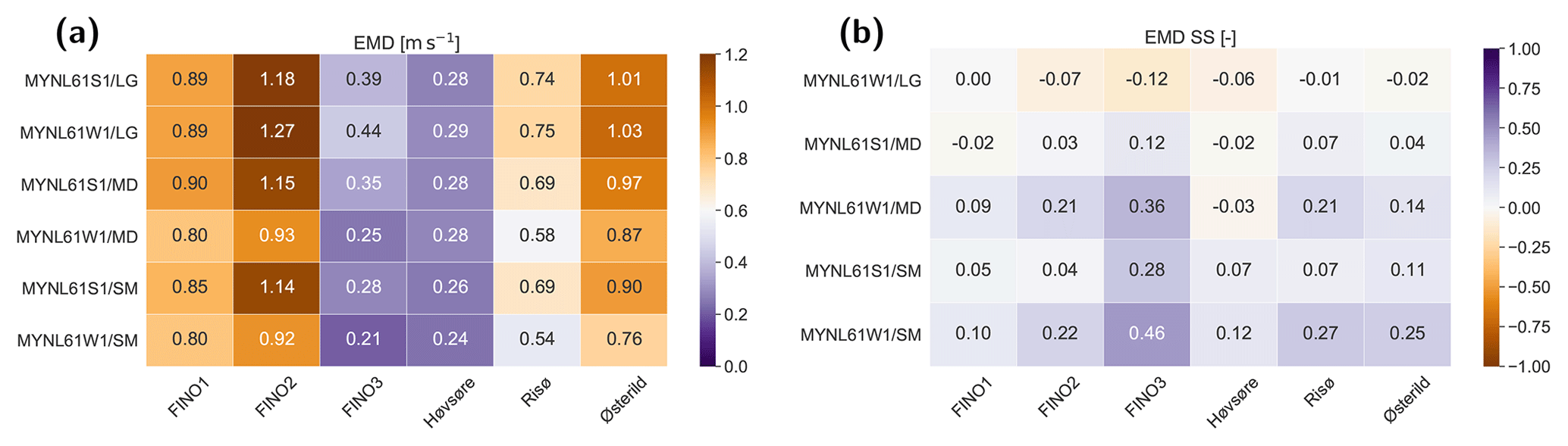
Figure 12 (a) EMD (m s⁻¹) and (b) EMD SS (–) between the observed and simulated wind speed for the six inner sites and underlined heights in Table 1 for the six domain size experiments. The EMD SS is compared to that of the EMD of the MYNL61W1/SM simulation.

Figure  shows the EMD between the various WRF model simulations and the observations for the six sites. It should be noted that these EMD values are larger than those previously shown for the LSM, SL, PBL, and other ensembles. The reason for this is that the simulations were carried out with WRFV3.6.1 (see the brown line in Fig. c), and the measurements at FINO1 and FINO2 are more affected by the presence of neighbouring wind farms in 2016 than they were in 2015. The EMD from all simulations are summarized as follows: for five out of six sites the MYNL61W1/LG simulation have the largest EMD, and for all sites the MYNL61W1/SM simulation has the smallest EMD. Similar results (not shown) emerge for the bias and RMSE. In conclusion, for this region, biases in mean wind speed are influenced by the size (and possibly also location) of the domain, smaller domains have generally lower wind speeds and thus lower biases. This effect is most pronounced in the week-long nudged simulations. The RMSE increases with increasing domain size and integration time.

The results from these experiments guided the design of the NEWA domains for the production run. Instead of a single (or a few) very large domain, we chose to conduct the simulations in a rather large number of medium-sized domains. While generating different time series, overlapping areas in simulations generally show similar wind climates (Witha et al., 2019, Sect. 2.1.3). We decided against very small domains, which would add to the needed computational resources and the extra effort of dealing with hundreds of model domains and because most countries would be covered by multiple domains. It was desired that each country should be covered by only one domain to avoid edge differences in overlapping domains. The final domain configuration, which is presented in this paper's companion (Dörenkämper et al., 2020), fulfil this requirement for all countries except Norway, Sweden, and Finland, which are so elongated that a correspondingly large domain would be detrimental to the accuracy of the results.

5.7 Summary of the sensitivity experiments

A long list of sensitivity studies were carried out to identify a suitable configuration for the NEWA production run. Below is a summary of the findings.

1. In the initial sensitivity experiments, the largest differences in annual mean wind speed at 100 m in Fig. 4 and AGL/AMSL in Table 2 are between simulations using two PBL schemes (MYNN and YSU) and coincide with regions of high surface roughness in all domains over Europe. Over the sea, the differences could be traced to differences in atmospheric stability but were modest.

2. The weekly simulations using spectral nudging tend to perform better (lower bias, EMD, and RMSE) for the eight sites in northern Europe. The simulation using the MYNN scheme in the WRF model version 3.6.1 outperformed the simulations using the YSU scheme in this region.

3. The use of the WRF model V3.8.1 and the MYNN scheme increased the biases compared to observations at nearly all sites and most levels. A couple of settings, mynn_mixlength = 0 and COARE_OPT = 3.0, turn the MYNN scheme nearly back to the conditions in the WRF model version 3.6.1. However, above 100 m a.g.l. the modified MYNN scheme gives lower wind speeds than the one in WRFV3.6.1 at all sites.

4. A series of 25 experiments varying the land, PBL, and surface layer scheme (LSM–PBL–SL) shows a spread in the mean wind speed of about 1 m s⁻¹. When comparing to wind speed observations, most LSM–PBL–SL ensembles show negative biases over the ocean (except for FINO2) and positive biases over land, which are more consistent between sites than LSM–PBL–SL combinations. This likely reflects misrepresentation of the land surface around each site than deficiencies in the LSM–PBL–SL schemes themselves.

5. Changes to the WRF model lookup table for surface roughness length have large consequences for the simulated wind speed but are nearly invisible to the evaluation against the tall masts because these are located in areas away from those impacted by the changes.

6. The use of the EMD metric and the skill score helps clarify the comparison of the improvements between the various LSM–PBL–SL and the BASE simulation, especially if the bias is small. No simulation improves the EMD for all sites, and very few simulations improve the EMD metric at all, especially for the land sites. However, the MO simulation, which uses the NOAH, MYNN, and MO surface layer schemes, improves the results, SS > 0.1, at four of the eight sites and was finally chosen as the physical model configuration for the NEWA production run.

7. A set of additional sensitivity experiments changing the source of forcing data, SST, dynamic options, and other physical parameterizations shows smaller changes from the baseline simulation than the various LSM–PBL–SL experiments. Nearly all the changes have inconsequential effects on the simulation of the wind speed at wind turbine hub height. Only the simulation using the CAM radiation scheme showed improvements over the RRTMG scheme used in the baseline experiment. However, it was concluded that the modest improvements were not worth the additional expense of running this scheme in the production run.

8. A final set of experiments testing the effect of the size of the domain on the simulated wind speed error statistics showed, for a domain centred over Denmark, that the simulations using the smaller domain have lower wind speeds that compare better to measurements and that time correlations decrease with domain size. It is however unclear if this is a consequence of the domain size itself or the location of the main inflow boundary to the domain in the simulations.

6 Discussion and outlook

In the companion paper (Dörenkämper et al., 2020) we document the final model configuration and how we computed the final wind atlas, including a detailed description of the technical and practical aspects that went in to running the WRF simulations and the downscaling using the linearized microscale model WAsP (Troen and Petersen, 1989). The companion paper also shows a comprehensive evaluation of each component of the NEWA model chain using observations from a large set (n=291) of tall masts located all over Europe. That work concludes that the NEWA wind climate estimated by the WRF model simulations using the model configuration selected here is significantly more accurate than using the raw ERA5 wind speed and direction which was used to force these simulations.

From the results of the sensitivity analysis, it is clear that some model setups have better scores for one validation metric (e.g. EMD) and some setups have better scores in other metrics (e.g. RMSE). Also, the performance of the setup varies considerably from station to station. In addition, one can clearly see that the performance at each station is systematic. At some sites all setups tend to perform better and at other sites worse. Thus, it was decided not to base configuration decisions on average metrics across the sites. From the results of the sensitivity analysis, several model setups could have been chosen (e.g. MO, SLAB, or CAMRAD). The MO setup, which was ultimately chosen for the production runs (Dörenkämper et al., 2020), is one of the best performing, according to the verification results. It performs well in terms of its wind speed distribution (EMD) and relatively well in a time series sense (RMSE) compared to other model setups. It has the additional benefit of runs being numerically stable when compared to BASE, i.e. the runs failed less (this aspect was important because of the necessity for a person to monitor and resubmit the runs), and MO also had a favourably small computational time when compared to other setups.

Many other details of the model setup have not been tested. For example, the sensitivity of the simulated wind climate to the number and location of the vertical levels in the PBL was not systematically tested. Previous studies (Hahmann et al., 2015) and earlier simulations in the NEWA project showed a small impact, but these were conducted with a single PBL scheme. The dependence of the simulated wind climate on the grid spacing is also not explored here. Previous publications offshore (e.g. Floors et al., 2018b) and onshore (Rife and Davis, 2005; Gómez-Navarro et al., 2015; Smith et al., 2018) have done so, but the investigation into what the ideal grid spacing of the mesoscale simulations is when further downscaling is done also remains unknown. Similarly, the dependence of the WRF model simulation of the wind climate on the size and location of the computational domain also remains unresolved. Smaller domains in the WRF simulation tend to have smaller wind speed biases and higher RMSE compared to tall mast observations, but it was unclear if this was really a result of the size of the domain or rather the location of the boundaries in relation to the large-scale flow. More numerical experiments should be carried out to identify all these potential interactions.

As with any modelling study, some questions remain unresolved simply because of the expensive nature of the numerical experiments. For convenience and simplicity, we separated the sensitivity experiments dealing with LSM–PBL–SL and the other parameterizations, changing only one scheme or parameter at a time. However, the experiment using the CAM radiation scheme had better verification statistics than the other simulations. The use of the CAM scheme was not tested using the preferred LSM–PBL–SL combination. Thus, we suggest that a better way to go in this process of model selection is to go through the changes and evaluation in a sequential way. However, the number of ensemble members can rapidly become unmanageable. Algorithms in this direction are currently being applied for tuning Earth System Models (Li et al., 2019) and could perhaps be evaluated to best determine the best suited WRF setups for different applications, not just wind resource assessment.

Finally, we have not evaluated the results of the ensemble simulations with the large observational dataset used in the companion paper (Dörenkämper et al., 2020). We also have not evaluated the simulated wind climatologies when we use the full downscaling model chain. Nevertheless, the evaluation of the production run with the data included there supports the performance of the configuration selected herein.

Appendix A

(Danielson and Gesch, 2011)(Copernicus Land Monitoring Service, 2019)(Poulter et al., 2015)(Hersbach et al., 2020)(OSTIA, Donlon et al., 2012)(Hong et al., 2004)(Kain, 2004)(Nakanishi and Niino, 2009)(Nakanishi and Niino, 2009)(Tewari et al., 2004)(Iacono et al., 2008)

Table A1 The WRF model setup common to all simulations and to the BASE simulation.

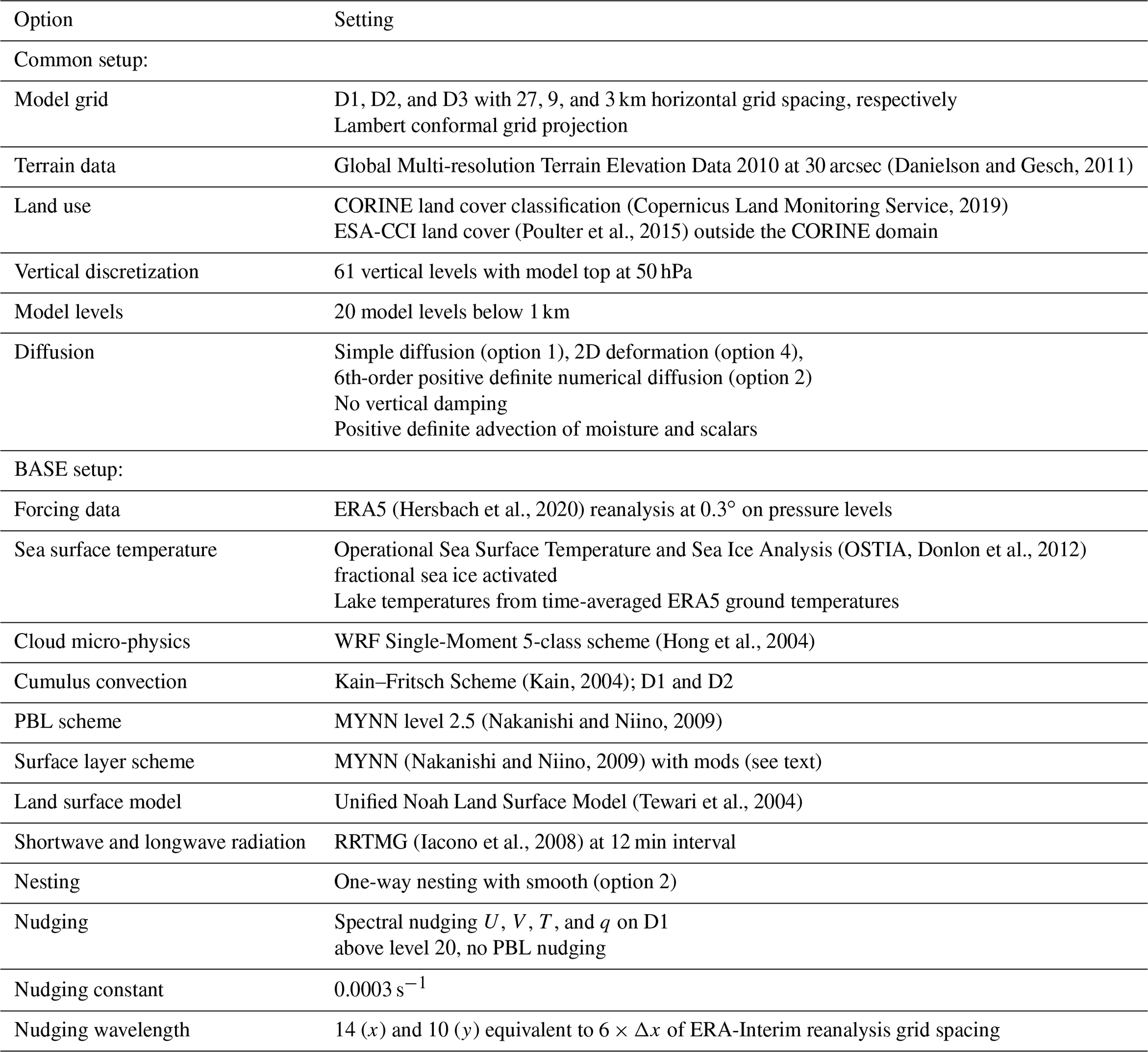
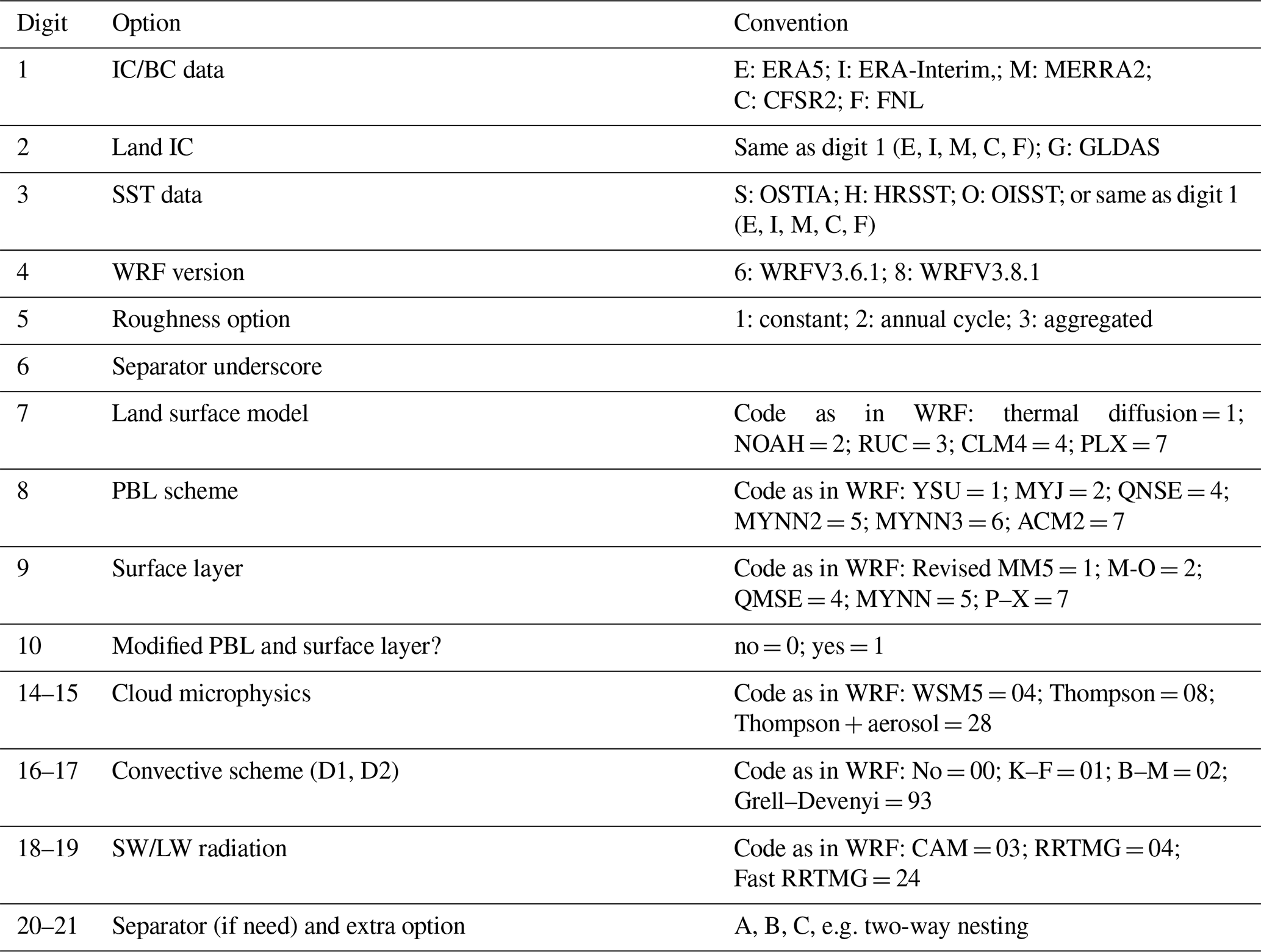
Table A2 Explanation for the various digits of the sensitivity experiments that refers to the code available in GitHub.