Simulating human impacts on global water resources using VIC-5

Questions related to historical and future water resources and scarcity have been addressed by several macroscale hydrological models. One of these models is the Variable Infiltration Capacity (VIC) model. However, further model developments were needed to holistically assess anthropogenic impacts on global water resources using VIC.

Our study developed VIC-WUR, which extends the VIC model using (1) integrated routing, (2) surface and groundwater use for various sectors (irrigation, domestic, industrial, energy, and livestock), (3) environmental flow requirements for both surface and groundwater systems, and (4) dam operation. Global gridded datasets on sectoral demands were developed separately and used as an input for the VIC-WUR model.

Simulated national water withdrawals were in line with reported Food and Agriculture Organization (FAO) national annual withdrawals (adjusted R² > 0.8), both per sector and per source. However, trends in time for domestic and industrial water withdrawal were mixed compared with previous studies. Gravity Recovery and Climate Experiment (GRACE) monthly terrestrial water storage anomalies were well represented (global mean root-mean-squared error, RMSE, values of 1.9 and 3.5 mm for annual and interannual anomalies respectively), whereas groundwater depletion trends were overestimated. The implemented anthropogenic impact modules increased simulated streamflow performance for 370 of the 462 anthropogenically impacted Global Runoff Data Centre (GRDC) monitoring stations, mostly due to the effects of reservoir operation. An assessment of environmental flow requirements indicates that global water withdrawals have to be severely limited (by 39 %) to protect aquatic ecosystems, especially with respect to groundwater withdrawals.

VIC-WUR has potential for studying the impacts of climate change and anthropogenic developments on current and future water resources and sector-specific water scarcity. The additions presented here make the VIC model more suited for fully integrated worldwide water resource assessments.

1 Introduction

Questions related to historical and future water resources and scarcity have been addressed by several macroscale hydrological models over the last few decades (Liang et al., 1994; Alcamo et al., 1997; Hagemann and Gates, 2001; Takata et al., 2003; Krinner et al., 2005; Bondeau et al., 2007; Hanasaki et al., 2008b; van Beek and Bierkens, 2009; Best et al., 2011). Early efforts focused on the simulation of natural water resources and the impacts of land cover and climate change on water availability (Oki et al., 1995; Nijssen et al., 2001a, b). Recently, a larger focus has been on incorporating anthropogenic impacts, such as water withdrawals and dam operations, into water resource assessments (Alcamo et al., 2003; Haddeland et al., 2006b; Biemans et al., 2011; Wada et al., 2011b; Hanasaki et al., 2018).

Global water withdrawals have increased 8-fold over the last century and are projected to increase further (Shiklomanov, 2000; Wada et al., 2011a). Although water withdrawals are only a small fraction of the total global runoff (Oki and Kanae, 2006), water scarcity can be severe due to the variability of water in both time and space (Postel et al., 1996). Severe water scarcity is already experienced by two-thirds of the global population for at least part of the year (Mekonnen and Hoekstra, 2016). To stabilize water availability for different sectors (e.g. irrigation, hydropower, and domestic uses), dams and reservoirs have been built, which are able to strongly affect global river streamflow (Nilsson et al., 2005; Grill et al., 2019). In addition, groundwater resources are being extensively exploited to meet increasing water demands (Rodell et al., 2009; Famiglietti, 2014).

One of the widely used macroscale hydrological models is the Variable Infiltration Capacity (VIC) model. This model was originally developed as a land surface model (Liang et al., 1994), but it has mostly been used as a stand-alone hydrological model (Abdulla et al., 1996; Nijssen et al., 1997) using an offline routing module (Lohmann et al., 1996, 1998a, b). Where land surface models focus on the vertical exchange of water and energy between the land surface and the atmosphere, hydrological models focus on the lateral movement and availability of water. By combining these two approaches, VIC simulations are strongly process based; this provides a good basis for climate-impact modelling.

VIC has been used extensively in studies such as coupled regional climate model simulations (Zhu et al., 2009; Hamman et al., 2016), combined river streamflow and water temperature simulations (van Vliet et al., 2016), hydrological sensitivity to climate change research (Hamlet and Lettenmaier, 1999; Nijssen et al., 2001a; Chegwidden et al., 2019), global streamflow simulations (Nijssen et al., 2001b), flow regulation and redistribution research (Voisin et al., 2018; Zhou et al., 2018), and real-time drought forecasting (Wood and Lettenmaier, 2006; Mo, 2008). Several studies have also used VIC to simulate the anthropogenic impacts of irrigation and dam operation on water resources (Haddeland et al., 2006a, b; Zhou et al., 2015, 2016) based on the model set-up of Haddeland et al. (2006b). However, further developments were needed to holistically assess anthropogenic impacts on global water resources using this model (Nazemi and Wheater, 2015a, b; Döll et al., 2016; Pokhrel et al., 2016).

Firstly, the VIC model did not include groundwater withdrawals or water withdrawals from domestic, manufacturing, and energy (thermoelectric) sources. Although these sectors use less water than irrigation (Shiklomanov, 2000; Grobicki et al., 2005; Hejazi et al., 2014), they are important actors locally (Gleick et al., 2013), especially for the water–food–energy nexus (Bazilian et al., 2011). Sufficient water supply and availability are essential for meeting a range of local and global sustainable development goals related to water, food, energy, and ecosystems (Bijl et al., 2018). Secondly, environmental flow requirements (EFRs) have often been neglected (Pastor et al., 2014), even though they are “necessary to sustain aquatic ecosystems which, in turn, support human cultures, economies, sustainable livelihoods, and well-being” (Arthington et al., 2018). Anthropogenic alterations already strongly affect freshwater ecosystems (Carpenter et al., 2011), with more than a quarter of all global rivers experiencing very high biodiversity threats (Vorosmarty et al., 2010). By neglecting EFRs, the sustainable water availability for anthropogenic uses is overestimated (Gerten et al., 2013). Lastly, while the model set-up of Haddeland et al. (2006b) already included important anthropogenic impact modules (i.e. irrigation and dam operation), these were not fully integrated. Therefore, multiple successive model runs were required (see Sect. 2.1), which was computationally expensive – especially for global water resources assessments.

Recently, version 5 of the VIC model (VIC-5) was released (Hamman et al., 2018), which focused on improving the VIC model infrastructure. These improvements provide the opportunity to fully integrate anthropogenic impacts into the VIC model framework while also reducing computation times. Here, the newly developed VIC-WUR model is presented (named after the development team at Wageningen University and Research). The VIC-WUR model extends the existing VIC-5 model using several modules that simulate the anthropogenic impacts on water resources. These modules will implement previous major works on anthropogenic impact modelling and will also integrate environmental flow requirements into VIC-5. The modules include the following: (1) integrated routing, (2) surface and groundwater use for various sectors (irrigation, domestic, industrial, energy, and livestock), (3) environmental flow requirements for both surface and groundwater systems, and (4) dam operation.

The next section first describes the original VIC-5 hydrological model (Sect. 2.1), which calculates natural water resource availability. Subsequently, the integration of the anthropogenic impact modules, which modify the water resource availability, is described (Sect. 2.2). Global anthropogenic water uses for each sector are also estimated (Sect. 2.3). To assess the capability of the newly developed modules, the VIC-WUR results were compared with Food and Agriculture Organization (FAO) national water withdrawals by sector and by source (FAO, 2016); with Huang et al. (2018), Steinfeld et al. (2006), and Shiklomanov (2000) data on water withdrawals by sector; with Gravity Recovery and Climate Experiment (GRACE) terrestrial water storage anomalies (NASA, 2002); with Global Runoff Data Centre (GRDC) streamflow time series (GRDC, 2003); and with Yassin et al. (2019) and Hanasaki et al. (2006) data on reservoir operation (Sect. 3.2). VIC-WUR simulation results are also compared with various other state-of-the-art global hydrological models. Lastly, the impacts of adhering to surface and groundwater environmental flow requirements on water availability are assessed (Sect. 3.3). This assessment is included to indicate the effects of the newly integrated surface and groundwater environmental flow requirements on worldwide water availability.

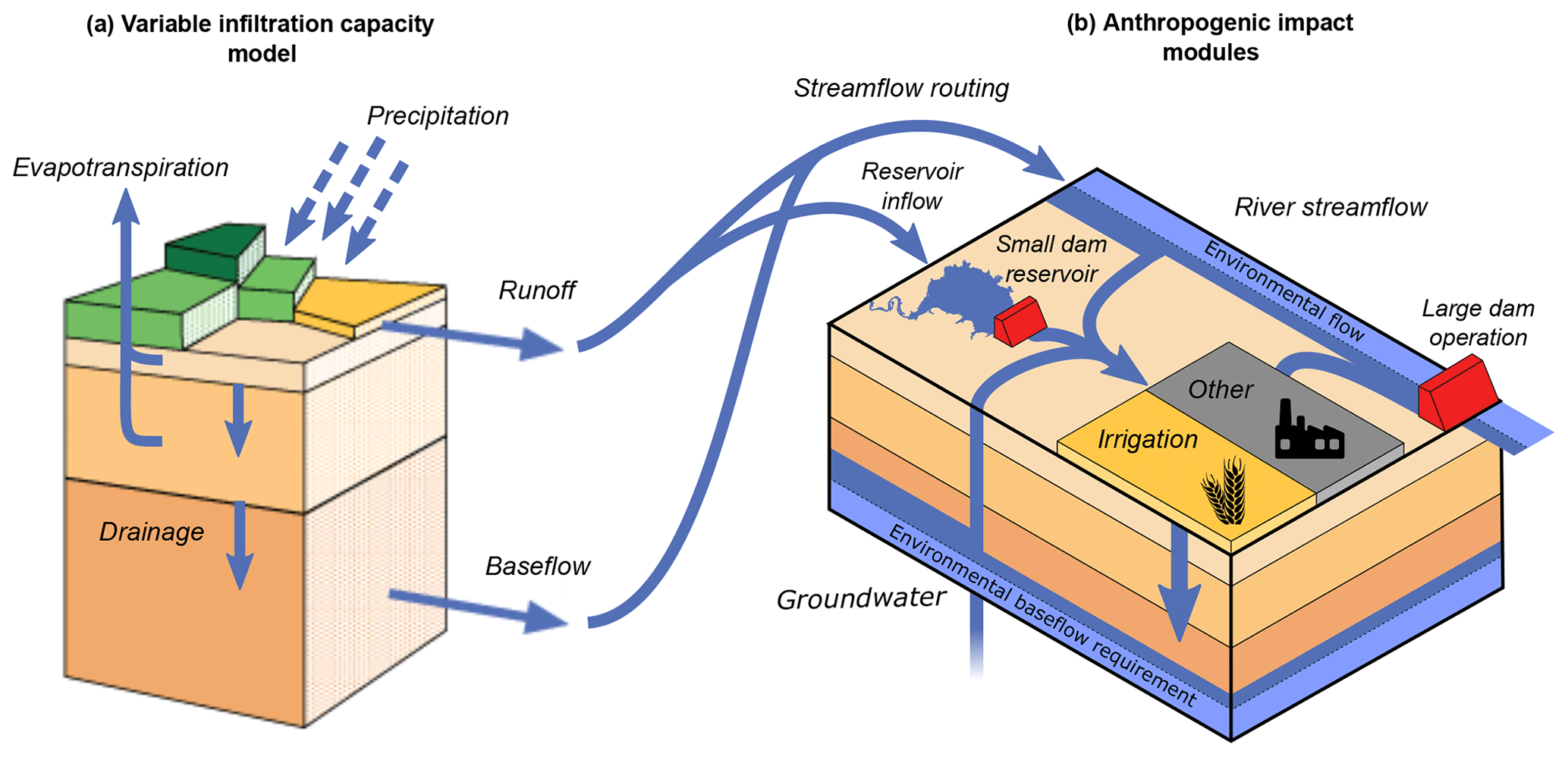
Figure 1 Schematic overview of the VIC-WUR model that includes the VIC-5 model (a) and several anthropogenic impact modules (b). Water from river streamflow, groundwater, and small (within-grid) reservoirs is available for withdrawal. Surface and groundwater withdrawals are constrained by environmental flow requirements. Withdrawn water is available for irrigation, domestic, industrial, energy, and livestock use. Unconsumed irrigation water is returned to the soil column of the hydrological model. Unconsumed water for the other sectors is returned to the river streamflow. Small reservoirs fill using surface runoff from the cell that they are located in, whereas large dam reservoirs operate solely on rivers' streamflow.

2 Model development

2.1 VIC hydrological model

The basis of the VIC-WUR model is the Variable Infiltration Capacity model version 5 (VIC-5; Liang et al., 1994; Hamman et al., 2018). VIC-5 is an open-source macroscale hydrological model that simulates the full water and energy balance on a (latitude–longitude) grid. Each grid cell accounts for sub-grid variability in land cover and topography as well as allowing for variable saturation across the grid cell. For each sub-grid, the water and energy balance is computed individually (i.e. sub-grids do not exchange water or energy with one another). The methods used to calculate the water and energy balance are summarized in Appendix A and are mainly based on the work of Liang et al. (1994). For a description of the global calibration and validation of the water balance, the reader is referred to Nijssen et al. (2001b).

VIC version 5 (Hamman et al., 2018) upgrades did not change the model representation of physical processes, but they improved the model infrastructure. Improvements include the use of NetCDF (network common data form) for input and output processing and the implementation of parallelization through message passing interface (MPI). These changes increase computational speed and make VIC-5 better suited for (computationally expensive) global simulations. The most significant modification that enables new model applications is that VIC-5 also changed the processing order of the model. In previous versions, all time steps were processed for a single grid cell before continuing to the next cell (time before space). In VIC-5, all grid cells are processed before continuing to the next time step (space before time). This development allows for interaction between grid cells every time step, which is important for full integration of the anthropogenic impact modules, especially water withdrawals and dam operation.

For example, surface and subsurface runoff routing to produce river streamflow was typically done as a post-processing operation (Lohmann et al., 1996; Hamman et al., 2017a), due to the time-before-space processing order of previous versions. In order for reservoirs to account for downstream water demand, an irrigation demand initialization was required. This initialization could either be an independent offline dataset (Voisin et al., 2013) or multiple successive model runs (Haddeland et al., 2006b). As VIC-5 uses the space-before-time processing order, irrigation water demands and runoff routing could be simulated each time step. The routing post-process was replaced by our newly developed routing module, which simulates routing sequentially (upstream to downstream) based on the Lohmann et al. (1996) equations.

2.2 Anthropogenic impact modules

VIC-WUR extends the existing VIC-5 through the addition of several newly implemented anthropogenic impact modules (Fig. 1). These modules include sector-specific water withdrawal and consumption, environmental flow requirements for both surface and groundwater systems, and dam operation for large and small (within-grid) dams.

2.2.1 Water withdrawal and consumption

In VIC-WUR, sectoral water demands need to be specified for each grid cell (Sect. 2.3). To meet water demands, water can be withdrawn from river streamflow, small (within-grid) reservoirs, and groundwater resources. Streamflow withdrawals are abstracted from the grid cell discharge (as generated by the routing module), and reservoir withdrawals are abstracted from small dam reservoirs (located in the cell). Groundwater withdrawals are abstracted from the third-layer soil moisture and an (unlimited) aquifer below the soil column. Aquifer abstractions represent renewable and non-renewable abstractions from deep groundwater resources. Subsurface runoff is used to fill the aquifer if there is a deficit.

The partitioning of water withdrawals between surface and ground water resources is data driven (similar to e.g. Döll et al., 2012; Voisin et al., 2017; Hanasaki et al., 2018). Partitioning was based on the study by Döll et al. (2012), who estimated groundwater withdrawal fractions for each sector in around 15 000 national and subnational administrative units. These groundwater fractions were mainly based on information from the International Groundwater Resources Assessment Centre (IGRAC; https://www.un-igrac.org/, last access: 17 October 2020) database. Surface water withdrawals were partitioned between river streamflow and small reservoirs relative to water availability. Groundwater withdrawals were first withdrawn from the third soil layer, then from the (remaining) river streamflow resources, and, finally, from the groundwater aquifer. This order was implemented to avoid an overestimation of non-renewable groundwater withdrawals as a result of errors in the partitioning data. Aquifer withdrawals are additionally limited by the pumping capacity from Sutanudjaja et al. (2018), who estimated regional pumping capacities based on information from IGRAC.

Water can also be withdrawn from the river streamflow of other “remote” cells in delta areas. As rivers cannot split in the routing module, the model is unable to simulate the redistribution of water resources in dendritic deltas. Therefore, streamflow at the river mouth is available for use in delta areas (partitioned based on demand) to simulate the actual water availability. Delta areas were delineated by the global delta map from Tessler et al. (2015).

In terms of water allocation, under conditions where water demands cannot be met, water withdrawals are allocated to the domestic, energy, manufacturing, livestock, and irrigation sectors in that order. Withdrawn water is partly consumed, meaning the water evaporates and does not return to the hydrological model. Consumption rates were set at 0.15 for the domestic sector and 0.10 for the industrial sector, based on data from Shiklomanov (2000). The water consumption in the energy sector was based on Goldstein and Smith (2002) and varies per thermoelectric plant based on the fuel type and cooling system. For the livestock sector, the assumption was made that all withdrawn water is consumed. Unconsumed water withdrawals for these sectors are returned as river streamflow. For the irrigation sector, consumption was determined by the calculated evapotranspiration. Unconsumed irrigation water remains in the soil column and eventually returns as subsurface runoff.

2.2.2 Environmental flow requirements

Water withdrawals can be constrained by environmental flow requirements (EFRs). These EFRs specify the timing and quantity of water needed to support terrestrial river ecosystems (Smakhtin et al., 2004; Pastor et al., 2019). Surface and groundwater withdrawals are constrained separately in VIC-WUR, based on the EFRs for streamflow and baseflow respectively. EFRs for streamflow specify the minimum river streamflow requirements, whereas EFRs for baseflow specify the minimum subsurface runoff requirements (from groundwater to surface water). As baseflow is a function groundwater availability, baseflow requirements are used to constrain groundwater (including aquifer) withdrawals.

Various EFR methods are available (Smakhtin et al., 2004; Richter et al., 2012; Pastor et al., 2014). Our study used the variable monthly flow (VMF) method (Pastor et al., 2014) to calculate the EFRs for streamflows. VMF calculates the required streamflow as a fraction of the natural flow during high (30 %), intermediate (45 %), and low (60 %) flow periods, as described in Appendix B. The VMF method performed favourably compared with other hydrological methods, in 11 case studies where EFRs were calculated locally (Pastor et al., 2014). The advantage of the VMF method is that the method accounts for the natural flow variability, which is essential to support freshwater ecosystems (Poff et al., 2010).

EFR methods for baseflow have been rather underdeveloped compared with EFR methods for streamflow. However, a presumptive standard of 90 % of the natural subsurface runoff through time was proposed by Gleeson and Richter (2018), as described in Appendix B. This standard should provide high levels of ecological protection, especially for groundwater-dependent ecosystems. Note that part of the EFRs for baseflow are already captured in the EFRs for streamflow, especially during low-flow periods that are usually dominated by baseflows. However, the EFRs for baseflow specifically limit local groundwater withdrawals, whereas EFRs for streamflow include the accumulated runoff from upstream areas. Moreover, the chemical composition of groundwater-derived flows is inherently different, making them a non-substitutable water flow for environmental purposes (Gleeson and Richter, 2018).

2.2.3 Dam operation

Due to the lack of globally available information on local dam operations, several generic dam operation schemes have been developed for macroscale hydrological models to reproduce the effect of dams on natural streamflow (Haddeland et al., 2006a; Hanasaki et al., 2006; Zhao et al., 2016; Rougé et al., 2019; Yassin et al., 2019). In VIC-WUR, a distinction is made between “small” dam reservoirs (with an upstream area smaller than the cell area) and “large” dam reservoirs, similar to Hanasaki et al. (2018), Wisser et al. (2010), and Döll et al. (2009). Small dam reservoirs act as buckets that fill using surface runoff from the grid cell they are located in, and reservoirs' storage can be used for water withdrawals in the same cell. Large dam reservoirs are located in the main river and use the operation scheme of Hanasaki et al. (2006), as described in Appendix C.

The scheme distinguishes between two dam types: (1) dams that do not account for water demands downstream (e.g. hydropower dams or flood protection dams) and (2) dams that do account for water demand downstream (e.g. irrigation dams). For dams that do not account for demands, dam release is aimed at reducing annual fluctuations in discharge. For dams that do account for demands, dam release is additionally adjusted to provide more water during periods of high demand. The operation scheme was validated by Hanasaki et al. (2006) for 28 reservoirs and has been used in various other studies (Hanasaki et al., 2008b, 2018; Döll et al., 2009; Pokhrel et al., 2012; Voisin et al., 2013). Here, the scheme was adjusted slightly to account for monthly varying EFRs and to reduce overflow releases, which is described in Appendix C.

The Global Reservoir and Dam (GRanD) database (Lehner et al., 2011) was used to specify location, capacity, function (purpose), and construction year of each dam. The capacity of multiple (small and large) dams located in the same cell were combined.

2.3 Sectoral water demands

VIC-WUR water withdrawals are based on the irrigation, domestic, industry, energy, and livestock water demand in each grid cell. Water demands represent the potential water withdrawal, which is reduced when insufficient water is available. Irrigation demands were estimated based on the hydrological model, whereas water demands for other sectors were provided to the model as an input. Domestic and industrial water demands were estimated based on several socioeconomic predictors, whereas energy and livestock water demands were derived from power plant and livestock distribution data. Due to data limitations, the energy sector was incomplete, and energy water demands were partly included in the industrial water demands (which combined the remaining energy and manufacturing water demands). For more details concerning sectoral water demand calculations, the reader is referred to Appendix D.

2.3.1 Irrigation demands

Irrigation demands were set to increase soil moisture in the root zone so that water availability was not limiting crop evapotranspiration and growth. The exception is rice paddy irrigation (Brouwer et al., 1989), where irrigation was also supplied to keep the upper soil layer saturated. Water demands for rice paddy irrigation practices are relatively high compared with conventional irrigation practices due to increased evaporation and percolation. Therefore, the crop irrigation demands for these two irrigation practices were calculated and applied separately (i.e. in different sub-grids). Note that multiple cropping seasons are included based on the MIRCA2000 land use dataset (Portmann et al., 2010; see Sect. 3.1 in this paper for more details).

Total irrigation demands also included transportation and application losses. Note that transportation and application losses are not “lost” but rather returned to the soil column without being used by the crop. The water loss fraction was based on Frenken and Gillet (2012), who estimated the aggregated irrigation efficiency for 22 United Nations subregions. Irrigation efficiencies were estimated based on the difference between AQUASTAT-reported irrigation water withdrawals and calculated irrigation water requirements (Allen et al., 1998), using data on crop information (e.g. growing season and harvest area) from AQUASTAT.

2.3.2 Domestic and industrial demands

Domestic and industrial water withdrawals were estimated based on the gross domestic product (GDP) per capita and the gross value added (GVA) by industries respectively (from Bolt et al., 2018; Feenstra et al., 2015; and World Bank, 2010; see Appendix D in this paper for more details). These drivers do not fully capture the multitude of socioeconomic factors that influence water demands (Babel et al., 2007). However, the wide availability of data allows for the extrapolation of water demands to data-scarce regions and future scenarios (using studies such as Chateau et al., 2014).

Domestic water demands per capita (used for drinking, sanitation, hygiene, and amenity uses) were estimated in a similar fashion to Alcamo et al. (2003). Demands increased non-linearly with the GDP per capita due to the acquisition of water-using appliances as households become richer. A minimum water supply is needed for survival, and the saturation of water-using appliances sets a maximum on domestic water demands. Industrial water demands (used for cooling, transportation, and manufacturing) were estimated in a similar fashion to Flörke et al. (2013) and Voß and Flörke (2010). Industrial demands increased linearly with the GVA (as an indicator of industrial production). As industrial water intensities (i.e. the water use per production unit) vary widely between different industries (Flörke and Alcamo, 2004; Vassolo and Döll, 2005; Voß and Flörke, 2010), the average water intensity was estimated for each country. Both domestic and industrial water demands were also influenced by technological developments that increase water use efficiency over time, as in Flörke et al. (2013).

Domestic water demands varied monthly based on air temperature variability as in Huang et al. (2018), based on Wada et al. (2011b). Using this approach, water demands were higher in summer than in winter, especially for counties with strong seasonal temperature differences. Domestic water demand per capita was downscaled using the HYDE3.2 gridded population maps (Goldewijk et al., 2017). Industrial water demands were kept constant throughout the year. Industrial demands were downscaled from national to grid cell values using the NASA Back Marble night-time light intensity map (Roman et al., 2018). National industrial water demands were allocated based on the relative light intensity per grid cell for each country.

2.3.3 Energy and livestock demands

Energy water demands (used for the cooling of thermoelectric plants) were estimated using data from van Vliet et al. (2016). Water use intensity for generation (i.e. the water use per generation unit) was estimated based on the fuel and cooling system type (Goldstein and Smith, 2002), which was combined with the generation capacity. Note that the data only covered a selection of the total number of thermoelectric power plants worldwide. Around 27 % of the total (non-renewable) global installed capacity between 1980 and 2011 was included in the dataset due to lack of information on cooling system types for the majority of thermoelectric plants. To avoid double counting, energy water demands were subtracted from the industrial water demands.

Livestock water demands (used for drinking and animal servicing) were estimated by combining the Gridded Livestock of the World (GLW3) map (Gilbert et al., 2018) with the livestock water requirement reported by Steinfeld et al. (2006). Eight varieties of livestock were considered: cattle, buffaloes, horses, sheep, goats, pigs, chicken, and ducks. Drinking water demands varied monthly based on temperature as described by Steinfeld et al. (2006) – drinking water requirements were higher during higher temperatures.

3 Model application

3.1 Set-up

VIC-WUR results were generated between 1979 and 2016, excluding a spin-up period of 1 year (analysis period from 1980 to 2016). The model used a daily time step (with a 6-hourly time step for snow processes), and simulations were executed on a 0.5^∘ × 0.5^∘ grid (around 55 km at the Equator) with three soil layers per grid cell. Soil and (natural) vegetation parameters were the same as in Nijssen et al. (2001c; disaggregated to 0.5^∘), who used various sources to determine the soil (Cosby et al., 1984; Carter and Scholes, 1999) and vegetation parameters (Calder, 1993; Ducoudre et al., 1993; Sellers et al., 1994; Myneni et al., 1997).

Nijssen et al. (2001c) used the Advanced Very High Resolution Radiometer vegetation type database (Hansen et al., 2000) to spatially distinguish 13 land cover types. The land cover type “cropland” in the original land cover dataset was replaced by cropland extents from the MIRCA2000 cropland dataset (Portmann et al., 2010). MIRCA2000 distinguishes the monthly growing area(s) and season(s) of 26 irrigated and rain-fed crop types around the year 2000. Crop types were aggregated into three land cover types: rain-fed, irrigated, and rice paddy cropland. The natural vegetation was proportionally rescaled to make up for discrepancies between the natural vegetation and cropland extents.

Cropland coverage (the cropland area actually growing crops) varied monthly based on the crop growing areas of MIRCA2000. The remainder was treated as bare soil. Cropland vegetation parameters (e.g. leaf area index – LAI, displacement, vegetation roughness, and albedo) vary monthly based on the crop growing seasons and the development-stage crop coefficients of the Food and Agricultural Organization (Allen et al., 1998).

The latest WATCH forcing data ERA-Interim (aggregated to a 6-hourly temporal resolution), developed by the EU Water and Global Change (WATCH; Harding et al., 2011) project, was used as climate forcing (WFDEI; Weedon et al., 2014). The dataset provides gridded historical climatic variables of minimum and maximum air temperature, precipitation (as the sum of snowfall and rainfall, GPCC bias corrected), relative humidity, pressure, and incoming shortwave and longwave radiation.

For naturalized simulations, only the routing module was used. For the anthropogenic impact simulations, the sectoral water withdrawals and dam operation modules were turned on in the model simulations. For the EFR-limited simulations, water withdrawals and dam operations were constrained as described.

3.2 Validation and evaluation

In order to validate the VIC-WUR anthropogenic impact modules, water withdrawal, terrestrial total water storage anomalies, and streamflow and reservoir operation simulations were compared with observations. The validation specifically focused on the effects of the newly included anthropogenic impact modules, meaning that streamflow and total water storage anomaly results are shown for river basins that are strongly influenced by human activities. A general validation for streamflow and terrestrial total water storage anomalies (including basins with limited human activities) is shown in Appendix E.

3.2.1 Sectoral water withdrawals

Simulated global domestic, industrial, livestock, and irrigation mean water withdrawals were 310, 771, 36, and 2202 km³ yr⁻¹ respectively for the period from 1980 to 2016. Sectoral water withdrawals were compared with FAO national annual water withdrawals (FAO, 2016), monthly withdrawal data from Huang et al. (2018), and annual withdrawal data from Shiklomanov (2000) and Steinfeld et al. (2006). For the latter studies, water withdrawals were aggregated by region (world, Africa, Asia, Americas, Europe, and Oceania). Note that Huang et al. (2018) irrigation water withdrawals integrate the results of four other macroscale hydrological models (WaterGAP, H08, LPJmL, and PCR-GLOBWB), using the same land use and climate set-up as our study. Results from individual macroscale hydrological models are also shown.

Figure 2 Comparison between simulated national annual water withdrawals and the FAO-reported values for the (a) domestic, (b) industrial, and (c) irrigation sectors. Colours distinguish between regions. Open circles were also used in the calibration of the water withdrawal demands. The dashed line indicates the 1:1 ratio, and the dotted line indicates the simulated best linear fit. Note the log–log axis which is used to display the wide range of water withdrawals. The adjusted R² is also based on the log values.

Simulated domestic, industrial, and irrigation water withdrawals correlated well with reported national water withdrawals, with an adjusted R² of 0.93, 0.94, and 0.82 for domestic, industrial, and irrigation water withdrawals respectively (Fig. 2a, b, c). Generally, smaller water withdrawals were overestimated and larger water withdrawals were underestimated. Differences for the domestic and industrial sector were small and probably related to the fact that smaller countries were poorly delineated on a 0.5^∘ × 0.5^∘ grid. However, irrigation differences were larger with overestimations of the irrigation water withdrawals in (mostly) Europe. As irrigation water demands are the result of the simulated water balance, overestimations would indicate a regional underestimation of the water availability for Europe or differences in irrigation efficiency.

When domestic, industrial, and livestock water withdrawals were compared to other studies, results were mixed (Fig. 3a, b, c). Simulated domestic withdrawals followed a similar trend in time. However, simulated domestic water withdrawal trends were somewhat underestimated overall, with a mean bias of 54 km³ yr⁻¹ compared with Huang et al. (2018). Asia is the main contributor to the global underestimation, but results are similar in most regions. The simulated industrial water withdrawal was (mostly) higher in our study, with a mean bias of 107 km³ yr⁻¹ compared with Huang et al. (2018) but only a mean bias of 5 km³ yr⁻¹ compared with Shiklomanov (2000). Moreover, industrial water withdrawal trends in time were less consistent.

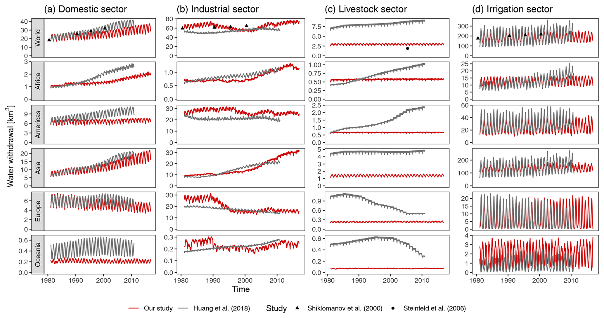
Figure 3 Comparison between the simulated monthly regional water withdrawal and values from Huang et al. (2018), Shiklomanov (2000), and Steinfeld et al. (2006) for the (a) domestic, (b) industrial, (c) livestock, and (d) irrigation sectors. Colours and shapes distinguish between studies. Note that the jitter in livestock withdrawals is due to the different days per month.

Withdrawal differences for the domestic and industrial sector are probably due to the limited data availability. Our approach to compute water demands was data-driven and sensitive to data gaps (as opposed to Huang et al., 2018, who also combined model results). For example, domestic withdrawal data for China were not available before 2007, and industrial withdrawal data were limited before 1990. Moreover, data on the disaggregation of industrial sectors (e.g. energy and mining), which can be important sectors in the water–food–energy nexus, were limited.

For livestock water withdrawals, there is a large discrepancy between Huang et al. (2018) and Steinfeld et al. (2006). Both studies used similar livestock maps, but there was large differences in livestock water intensity (in units of litres per animal per year). As our study used values from Steinfeld et al. (2006) to estimate livestock water intensity, our results were closer to their values (slightly higher due to the inclusion of buffaloes, horses, and ducks). Note that Huang et al. (2018) shows trends in livestock water withdrawals, whereas our study uses static livestock maps.

Simulated irrigation water withdrawals were within the range of other macroscale hydrological model estimates (Table 1). Simulated monthly variability in irrigation water withdrawals is reduced compared with the compiled results of Huang et al. (2018) (Fig. 3d), especially in Asia. Moreover, trends in time are less pronounced, as can be seen in Africa. These differences may indicate a relative low weather or climate sensitivity of evapotranspiration in VIC-WUR, as annual and interannual weather changes affect irrigation water demands to a lesser degree.

Table 1 Average annual global irrigation water withdrawals as calculated by several global hydrological models.

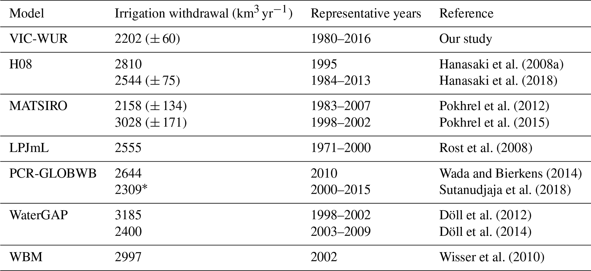
^* Includes livestock withdrawals.

3.2.2 Groundwater withdrawals and depletion

Simulated global mean surface and groundwater withdrawals were 2327 and 992 km³ yr⁻¹ respectively for the period from 1980 to 2016. Of the global groundwater withdrawals, 334 km³ yr⁻¹ contributed to groundwater depletion. Simulated ground and surface water withdrawals and terrestrial total water storage anomalies were compared with FAO national annual water withdrawals (FAO, 2016) and monthly storage anomaly data from the GRACE satellite (NASA, 2002). GRACE satellite total water storage anomalies were used to validate total water storage dynamics as well as groundwater exploitation contributing to downward trends in total water storage. Groundwater depletion results from other macroscale hydrological models are shown as well. In order to compare the simulation results to the GRACE dataset, a 300 km Gaussian filter was applied to the simulated data (similar to Long et al., 2015).

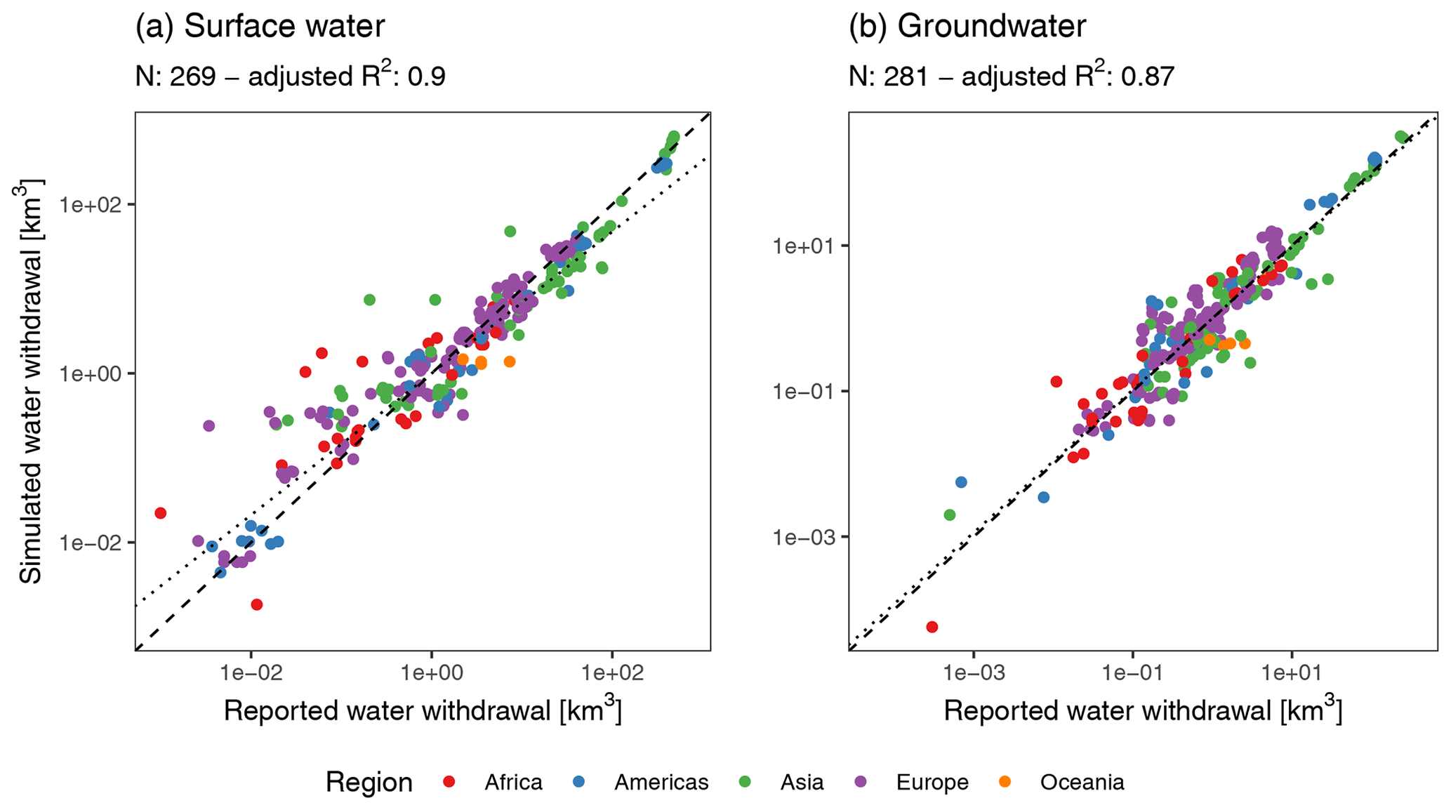
Figure 4 Comparison between simulated national annual water withdrawals and FAO-reported values from (a) surface water and (b) groundwater. Colours distinguish between regions. The dashed line indicates the 1:1 ratio, and the dotted line indicates the simulated best linear fit. Note the log–log axis which is used to display the wide range of water withdrawals. The adjusted R² is also based on the log values.

Simulated surface and groundwater withdrawals correlated well with the reported national water withdrawals, with an adjusted R² of 0.90 and 0.87 for surface and groundwater respectively (Fig. 4a, b). Surface water withdrawals were overestimated for low withdrawals and underestimated for large withdrawals. There is a weak correlation (−0.35) between the underestimations in surface water withdrawals and the overestimation in groundwater withdrawals, meaning water withdrawal differences could be related to the partitioning between surface and groundwater resources. Furthermore, it is likely that low water demands are overestimated (as discussed in Sect. 3.2.1), resulting in an overestimation of low surface water withdrawals.

Simulated monthly terrestrial water storage anomalies correlated well with the GRACE observations, with a mean annual and interannual root-mean-squared error (RMSE) of 1.9 and 3.5 mm respectively. The difference between annual and interannual performance was primarily due to the groundwater depletion process (Fig. 5). Simulated groundwater depletion was (mostly) overestimated (e.g. Indus and Hai He basins), with higher declining trends in terrestrial total water storage for most basins. However, the simulated groundwater withdrawal and exploitation was within range compared with other macroscale hydrological models (Table 2), even though total groundwater withdrawals were relatively high.

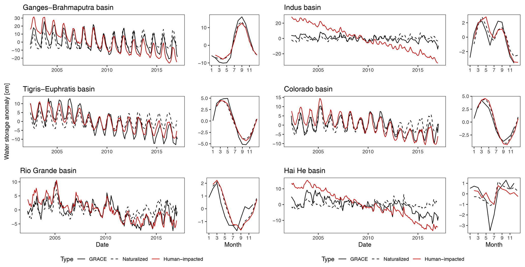
Figure 5 Comparison between simulated monthly terrestrial total water storage anomalies and GRACE-observed values. Panels indicate the time series and multiyear mean averages for naturalized simulations (dashed), anthropogenically impacted simulations (red), and observed (black) terrestrial total water storage anomalies.

Table 2 Average annual global groundwater withdrawals and depletion as calculated by several global hydrological models.

As with the FAO comparison, these results seems to indicate that withdrawal partitioning towards groundwater is overestimated. However, conclusions regarding groundwater depletion are limited by the relatively simplistic approach to groundwater used in our study (as discussed by Konikow, 2011, and de Graaf et al., 2017). For example, processes such as wetland recharge and groundwater flows between cells are not simulated, even though these could decrease groundwater depletion.

3.2.3 Discharge modification

Simulated discharge was compared to GRDC station data (GRDC, 2003) for various anthropogenically impacted rivers. Stations were selected if the upstream area was larger than 20 000 km², matched the simulated upstream area at the station location, and the available data spanned more than 2 years. Subsequently, stations where the anthropogenic impact modules did not sufficiently affect discharge were omitted. In order validate the reservoir operation more thoroughly, simulated reservoir inflow, storage, and release were compared with operation data from Hanasaki et al. (2006) and Yassin et al. (2019). Reservoirs were included if the simulated storage capacity (which is the combined storage capacity of all large dams in a grid) was similar to the observed storage capacity.

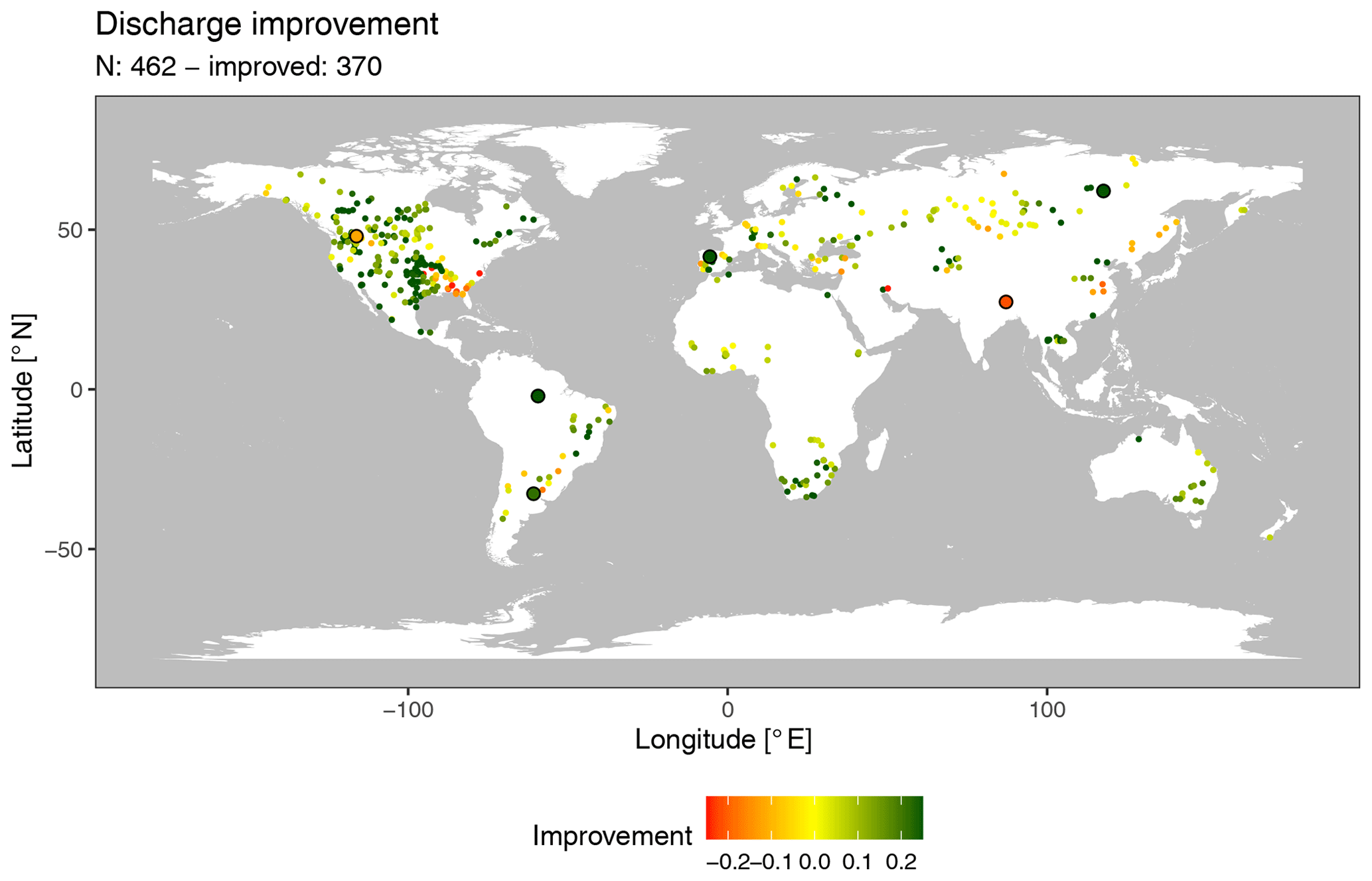
Figure 6 Discharge improvement from naturalized to anthropogenically impacted simulations (as a fraction of the naturalized RMSE). Circled larger stations are shown in Fig. 7.

Figure 7 Comparison between the simulated discharge and GRDC-observed values. Panels indicate the time series and multiyear averages for naturalized simulations (dashed), anthropogenically impacted simulations (red), and observed (black) discharge.

The inclusion of the anthropogenic impact modules improved discharge performance, measured in RMSE, for 370 of the 462 stations (80 %; Figs. 6, 7). Improvements were mainly due to the effects of reservoir operation on discharges (e.g. Cachoeira Morena and Suntar stations) but also due to withdrawal reductions (e.g. Tore station). However, reservoir effects on discharge were sometimes underestimated (e.g. Timbues station). Decreased performance was mostly related to under- or overestimations of (calibrated) natural streamflow which was subsequently exacerbated by reservoir operation and water withdrawals. For example, the Clark Fork River naturalized streamflow was underestimated, which was subsequently further underestimated by the anthropogenic impact modules (Whitehorse Rapids station). Moreover, increases in discharge due to groundwater withdrawals could increase naturalized streamflow (e.g. Turkeghat station). Further improvements to discharge performance would most likely require a recalibration of the VIC model parameters.

For individual reservoirs, operational characteristics were generally well simulated (Fig. 8), with reductions in annual discharge variations (e.g. Flaming Gorge and Garrison dams) and increased water release for irrigation (e.g. Seminoe Dam). However, due to changes in locally simulated and actual inflow, dam operation can take on different characteristics (e.g. Toktogul Dam). Furthermore, peak discharge events caused by reservoir overflow (as also described by Masaki et al., 2018) were not always sufficiently represented in the observations (e.g. Garrison Dam). These differences indicate locally varying reservoir operation strategies. Several studies have developed reservoir operation schemes that can be calibrated to the local situation (Rougé et al., 2019; Yassin et al., 2019). However, worldwide implementation of these operation schemes remains limited by data availability.

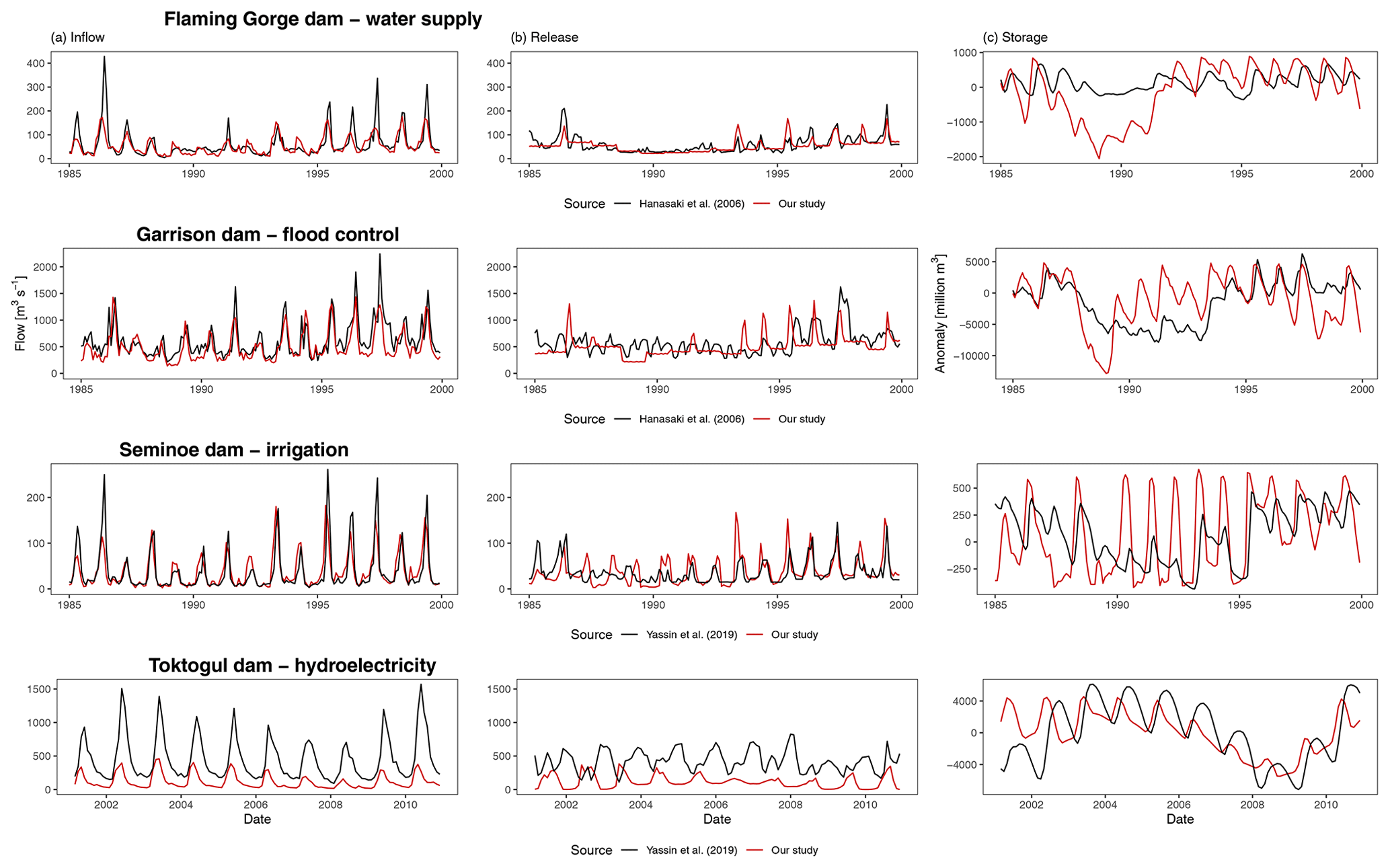
Figure 8 Comparison between the simulated reservoir operation and values observed by Hanasaki et al. (2006) and Yassin et al. (2019). Panels indicate the time series (a) inflow, (b) release, and (c) time series for anthropogenically impacted simulations (red) and observations (black).

3.3 Integrated environmental flow requirements

In order to assess the impact and capabilities of the newly integrated environmental flow requirements (EFRs) module, simulated water withdrawals with and without adhering to EFRs were compared.

If water use was limited to EFRs, irrigation withdrawals would need to be reduced by about 39 % (851 km³ yr⁻¹; Fig. 9a). Under the strict requirements used in our study, 81 % (693 km³ yr⁻¹) of the reduction could be attributed to limitations imposed on groundwater withdrawals. Subsequently, the impact of the environmental flow requirements (if adhered to) would be largest in groundwater-dependent regions (Fig. 9b). Note that downstream surface water withdrawals increase by 98 km³ yr⁻¹ when limiting groundwater water withdrawals, due to increased subsurface runoff in the integrated EFR module.

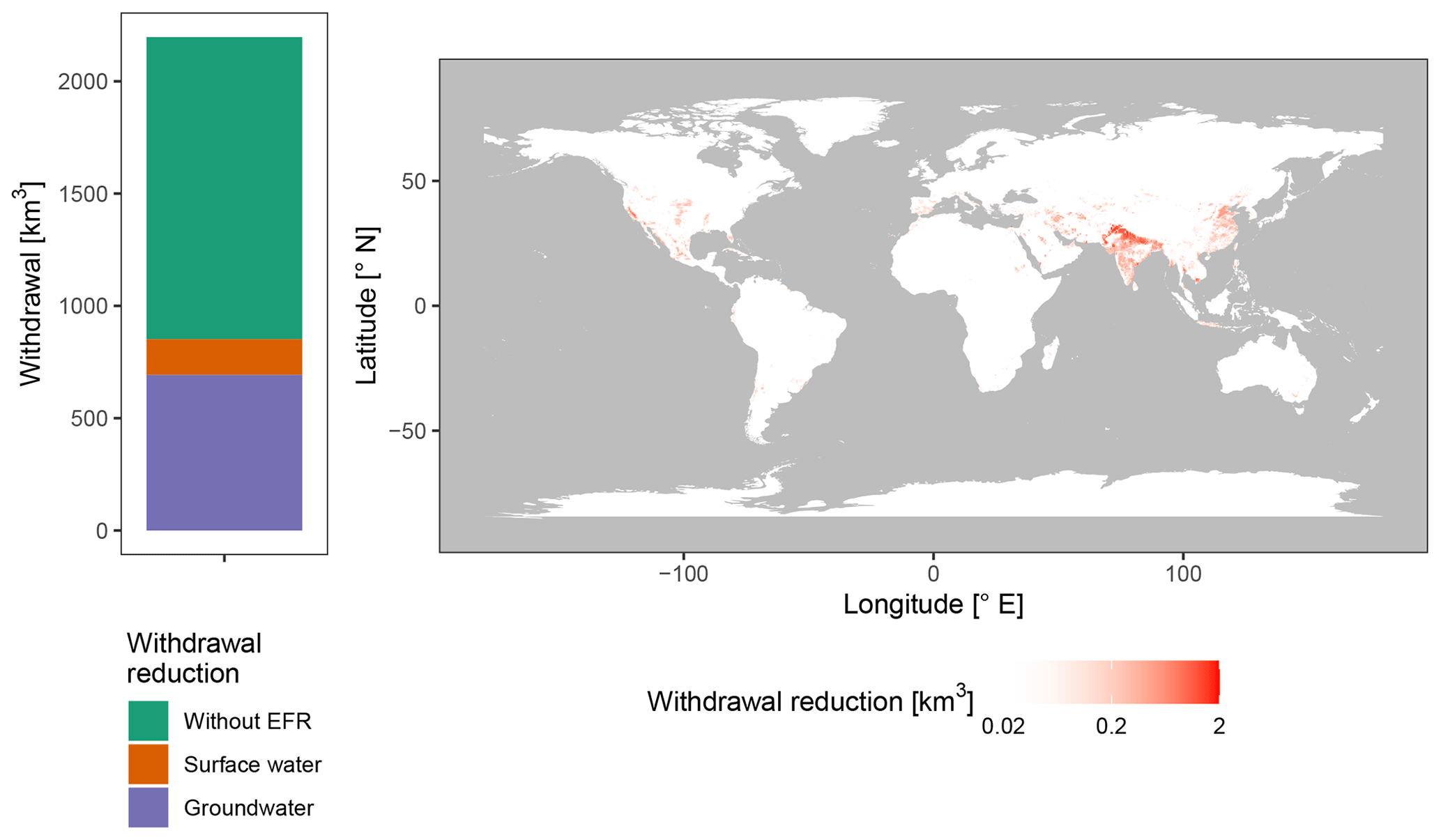
Figure 9 Average annual irrigation water withdrawal reductions when adhering to EFRs as a global gross total (a) and as spatially distributed values (b). Global gross totals are separated into withdrawals without any reduction (green), surface water withdrawal reductions (orange), and groundwater withdrawal reductions (purple). Note the log axis for the spatially distributed withdrawal reductions to better display the spatial distribution of the reductions.

Reductions due to EFRs were similar to Jägermeyr et al. (2017), who calculated irrigation withdrawal reductions of 41 % (997 km³ yr⁻¹) assuming only surface water abstractions. In our study, surface water reductions were smaller, as the strict groundwater requirements increase subsurface runoff to surface waters. The extent to which the EFRs for baseflow were overly constrictive can be discussed, as they were based on the relatively stringent EFR for streamflow from Richter et al. (2012) – 10 % of the natural streamflow. However, in the absence of any other standards, this baseflow standard remains the best available. Note that, even when accounting for EFRs for baseflow on a grid scale, withdrawals could still have local and long-term impacts that are not captured by the model. The timing, location, and depth of groundwater withdrawals are important factors due to their interactions with the local geohydrology, as discussed by Gleeson and Richter (2018).

4 Conclusions

The VIC-WUR model introduced in this paper aims to provide new opportunities for global water resource assessments using the VIC model. Accordingly, several anthropogenic impact modules, based on previous major works, were integrated into the VIC-5 macroscale hydrological model: domestic, industrial, energy, livestock, and irrigation water withdrawals from both surface water and groundwater as well as an integrated environmental flow requirement module and a dam operation module. Global gridded datasets on domestic, industrial, energy, and livestock demand were developed separately and used to force the VIC-WUR model.

Simulated national water withdrawals were in line with reported national annual withdrawals (adjusted R² > 0.8; both per sector and per source). However, the data-oriented methodology used to derive sectoral water demands resulted in different withdrawal trends over time compared with other studies (Shiklomanov, 2000; Huang et al., 2018). While the current set-up to estimate sectoral water demands is well suited for future water withdrawal estimations, there are various other approaches (e.g. Alcamo et al., 2003; Vassolo and Döll, 2005; Shen et al., 2008; Hanasaki et al., 2013; Wada and Bierkens, 2014). As the model set-up of VIC-WUR allows for the evaluation of other sectoral water demand inputs (on various temporal aggregations), several different approaches can be used depending on the focus region and data availability for calibration. Terrestrial water storage anomaly trends were well simulated (mean annual and interannual RMSE of 1.9 and 3.6 mm respectively), whereas groundwater exploitation was overestimated. Overestimated groundwater depletion rates are likely related to an over-partitioning of water withdrawals to groundwater. The implemented anthropogenic impact modules increased simulated discharge performance (at 370 of the 462 stations), mostly due to the effects of reservoir operation.

An assessment of the effect of EFRs shows that (when one adheres to these requirements) global water withdrawals would be severely limited (39 %). This limitation is especially notable for groundwater withdrawals, which, under the strict requirements used in our study, need to be reduced by 81 %. VIC-WUR has potential for studying impacts of climate change and anthropogenic developments on current and future water resources and sector-specific water scarcity. The additions presented here make the VIC model more suited for fully integrated worldwide water resource assessments and substantially decrease computation times compared with Haddeland et al. (2006a).

Appendix A: VIC water and energy balance

n VIC, each sub-grid computes the water and energy balance individually (i.e. sub-grids do not exchange water or energy with one another). For the water balance, incoming precipitation is partitioned between evapotranspiration, surface and subsurface runoff, and soil water storage. Potential evapotranspiration is based on the Penman–Monteith equation without the canopy resistance (Shuttleworth, 1993). The actual evapotranspiration is calculated using two methods, based on whether the land cover is vegetated or not (bare soil). Evapotranspiration of vegetation is constrained by stomatal, architectural, and aerodynamic resistances and is partitioned between canopy evaporation and transpiration based on the intercepted water content of the canopy (Deardorff, 1978; Ducoudre et al., 1993). Bare soil evaporation is constrained by the saturated area of the upper soil layer. The saturated area is variable within the grid, as (as the model name implies) the infiltration capacity of the soil is assumed to be heterogeneous (Franchini and Pacciani, 1991). Saturated areas evaporate at the potential evaporation rate, whereas evaporation is limited in unsaturated areas. Surface runoff is produced by precipitation over saturated areas. Precipitation over unsaturated areas infiltrates into the upper soil layer and drains through the soil layers based on the gravitational hydraulic conductivity equations of Brooks and Corey (1964). In the first and second layer, water is available for transpiration, while the third layer is assumed to be below the root zone. From the third layer, baseflow is generated based on the non-linear Arno conceptualization (Franchini and Pacciani, 1991). Baseflow increases linearly with soil moisture content when the moisture content is low. At higher soil moisture contents, the relation is non-linear, representing subsurface storm flows.

For the energy balance, incoming net radiation is partitioned between sensible, latent, and ground heat fluxes as well as energy storage in the air below the canopy. The energy storage below the canopy is omitted if it is considered negligible (e.g. the canopy surface is open or close to the ground). The latent heat flux is determined by the evapotranspiration as calculated in the water balance. The sensible heat flux is calculated based on the difference between the air and surface temperature, and the ground heat flux is calculated based on the difference between the soil and surface temperature. As the incoming net radiation is also a function of the surface temperature (specifically the outgoing longwave radiation), the surface temperature is solved iteratively. Subsurface ground heat fluxes are calculated assuming an exponential temperature profile between the surface and the bottom of the soil column, where the bottom temperature is assumed to be constant. Later model developments included options for finite difference solutions of the ground temperature profile (Cherkauer and Lettenmaier, 1999), the spatial distribution of soil temperatures (Cherkauer and Lettenmaier, 2003), a quasi-two-layer snowpack snow model (Andreadis et al., 2009), and blowing snow sublimation (Bowling et al., 2004).

Appendix B: EFRs for surface and groundwater

VIC-WUR used the variable monthly flow (VMF) method (Pastor et al., 2014) to limit surface water withdrawals. The VMF method (Pastor et al., 2014) calculates the EFRs for streamflow as a fraction of the natural flow during high (Eq. B3), intermediate (Eq. B2), and low (Eq. B1) flow periods. The presumptive standard from Gleeson and Richter (2018) is used to limit groundwater withdrawals (including aquifer groundwater withdrawals). This standard calculates the EFRs for baseflow as 90 % of the natural subsurface runoff through time (Eq. B4). Here, daily instead of monthly EFRs were used to better capture the monthly flow variability.

$$\begin{array}{}\text{(B1)}& {\displaystyle }\begin{array}{rl}{\text{EFR}}_{\text{s,d}}=& \mathrm{0.6}\cdot {\text{NF}}_{\text{s,d}}\\ & \text{where}{\text{NF}}_{\text{s,d}}\le \mathrm{0.4}\cdot {\text{NF}}_{\text{s,y}}\end{array}\text{(B2)}& {\displaystyle }\begin{array}{rl}{\text{EFR}}_{\text{s,d}}=& \mathrm{0.45}\cdot {\text{NF}}_{\text{s,d}}\\ & \text{where}\mathrm{0.4}\cdot {\text{NF}}_{\text{s,y}}<{\text{NF}}_{\text{s,d}}\le \mathrm{0.8}\cdot {\text{NF}}_{\text{s,y}}\end{array}\text{(B3)}& {\displaystyle }\begin{array}{rl}{\text{EFR}}_{\text{s,d}}=& \mathrm{0.3}\cdot {\text{NF}}_{\text{s,d}}\\ & \text{where}{\text{NF}}_{\text{s,d}}>\mathrm{0.8}\cdot {\text{NF}}_{\text{s,y}}\end{array}\text{(B4)}& {\displaystyle }{\text{EFR}}_{\text{b,d}}=\mathrm{0.9}\cdot {\text{NF}}_{\text{b,d}},\end{array}$$

where EFR_s,d is the daily EFRs for streamflow (m³ s⁻¹), EFR_b,d is the daily EFRs for baseflow (m³ s⁻¹), NF_s,d is the average natural daily streamflow (m³ s⁻¹), NF_s,y is the average natural yearly streamflow (m³ s⁻¹), and NF_b,d is the average natural daily baseflow (m³ s⁻¹). EFRs for streamflow and baseflow were based on VIC-WUR naturalized simulations between 1980 and 2010. Average natural daily flows were calculated as the interpolated multiyear monthly average flow over the simulation period.

Appendix C: Dam operation scheme

VIC-WUR used a dam operation scheme based on Hanasaki et al. (2006). Target release (i.e. the estimated optimal release) was calculated at the start of the operational year. The operational year starts at the month where the inflow drops below the average annual inflow and, thus, the storage should be at its desired maximum. The scheme distinguished between two dam types: (1) dams that did not account for water demands downstream (e.g. hydropower dams or flood control) and (2) dams that did account for water demands downstream (e.g. irrigation dams). The original scheme of Hanasaki et al. (2006) also accounts for EFRs, which were fixed at half the annual mean inflow. Other studies lowered the requirements to a 10th of the mean annual inflow, increasing irrigation availability and preventing excessive releases (Biemans et al., 2011; Voisin et al., 2013). In our study, the original dam operation scheme was adapted slightly to account for monthly varying EFRs.

For dams that did not account for demands, the initial release was set at the mean annual inflow corrected by the variable EFRs (Eq. C1). For dams that did account for demands, the initial release was increased during periods of higher water demand. If demands were relatively high compared with the annual inflow, the release was corrected by the demand relative to the mean demand (Eq. C2). If demands were relatively low compared with the annual inflow, release was corrected based on the actual water demand (Eq. C3).

$$\begin{array}{}\text{(C1)}& {\displaystyle }\begin{array}{rl}{R}_{\mathrm{m}}^{\prime }=& {\text{EFR}}_{\text{s,m}}+(I_{\mathrm{y}}-{\text{EFR}}_{\text{s,y}})\\ & \text{where}{D}_{\mathrm{y}}=\mathrm{0}\end{array}\text{(C2)}& {\displaystyle }\begin{array}{rl}{R}_{\mathrm{m}}^{\prime }=& {\text{EFR}}_{\text{s,m}}+(I_{\mathrm{y}}-{\text{EFR}}_{\text{s,y}})\cdot {\displaystyle \frac{D_{\mathrm{m}}}{D_{\mathrm{y}}}}\\ & \text{where}{D}_{\mathrm{y}}>\mathrm{0}\text{and}{D}_{\mathrm{y}}>(I_{\mathrm{y}}-{\text{EFR}}_{\text{s,y}})\end{array}\text{(C3)}& {\displaystyle }\begin{array}{rl}{R}_{\mathrm{m}}^{\prime }=& {\text{EFR}}_{\text{s,m}}+(I_{\mathrm{y}}-{\text{EFR}}_{\text{s,y}})-D_{\mathrm{y}}+D_{\mathrm{m}}\\ & \text{where}{D}_{\mathrm{y}}>\mathrm{0}\text{and}{D}_{\mathrm{y}}\le (I_{\mathrm{y}}-{\text{EFR}}_{\text{s,y}}),\end{array}\end{array}$$

where $R_{\mathrm{m}}^{\prime }$ is the initial monthly target release (m³ s⁻¹), EFR_s,m is the average monthly EFR for streamflow demand (m³ s⁻¹), I_y is the average yearly inflow (m³ s⁻¹), EFR_s,y is the average yearly EFR for streamflow (m³ s⁻¹), D_m is the average monthly water demand (m³ s⁻¹), and D_y is the average yearly water demand (m³ s⁻¹).

As in Hanasaki et al. (2006), the initial target release was adjusted based on storage and capacity. Target release was adjusted to compensate for differences between the current storage and the desired maximum storage (Eq. C4). Target release was additionally adjusted if the storage capacity was relatively low compared with the annual inflow and was unable to store large portions of the inflow for later release (Eq. C5).

$$\begin{array}{}\text{(C4)}& {\displaystyle }\begin{array}{rl}{R}_{\mathrm{m}}=& k\cdot R_{\mathrm{m}}^{\prime }\\ & \text{where}c\ge \mathrm{0.5}\end{array}\text{(C5)}& {\displaystyle }\begin{array}{rl}{R}_{\mathrm{m}}=& {\left({\displaystyle \frac{c}{\mathrm{0.5}}}\right)}^{\mathrm{2}}\cdot k\cdot R_{\mathrm{m}}^{\prime }+\left\{\mathrm{1}-{\left({\displaystyle \frac{c}{\mathrm{0.5}}}\right)}^{\mathrm{2}}\right\}\cdot I_{\mathrm{m}}\\ & \text{where}\mathrm{0}\le c\le \mathrm{0.5},\end{array}\end{array}$$

where I_m is the average monthly inflow (m³ s⁻¹), c is the capacity parameter (–) calculated as the storage capacity divided by the mean annual inflow, and k is the storage parameter (–) calculated as current storage divided by the desired maximum storage. The desired maximum storage was set at 85 % of the storage capacity, as recommended by Hanasaki et al. (2006).

Water inflow, demand and EFRs were estimated based on the average of the past 5 years. Water demands were based on the water demands of downstream cells. Only a fraction of water demands were taken into account, based on the fraction of discharge the dam controlled. For example, if a dam controlled 70 % of the discharge of a downstream cell, 70 % of its demands were taken into account. Fractions smaller than 25 % were ignored.

The original dam operation scheme of Hanasaki et al. (2006) was shown to produce excessively high discharge events due to overflow releases (Masaki et al., 2018). These overflow releases occurred due to a mismatch between the expected and actual inflow. In our study, dam release was increased during high-storage events to prevent overflow and the accompanying high discharge events. If dam storage was above the desired maximum storage, target dam release was increased to negate the difference (Eq. C6). If dam storage was below the desired minimum storage, release was decreased (Eq. C7). Dam release was adjusted exponentially based on the relative storage difference: small storage differences were only corrected slightly, but if the dam was close to overflowing or emptying, the difference was corrected strongly.

$$\begin{array}{}\text{(C6)}& {\displaystyle }\begin{array}{rl}{R}_{\mathrm{a}}=& R_{\mathrm{m}}+{\displaystyle \frac{(S-C\mathit{\alpha })}{\mathit{\gamma }}}\cdot {\left({\displaystyle \frac{\frac{S}{C}-\mathit{\alpha }}{\mathrm{1}-\mathit{\alpha }}}\right)}^b\\ & \text{where}S>C\mathit{\alpha }\end{array}\text{(C7)}& {\displaystyle }\begin{array}{rl}{R}_{\mathrm{a}}=& R_{\mathrm{m}}+{\displaystyle \frac{(S-C(\mathrm{1}-\mathit{\alpha }\left)\right)}{\mathit{\gamma }}}\cdot {\left({\displaystyle \frac{(\mathrm{1}-\mathit{\alpha })-{\displaystyle \frac{S}{C}}}{\mathrm{1}-\mathit{\alpha }}}\right)}^b\\ & \text{where}S<C(\mathrm{1}-\mathit{\alpha }),\end{array}\end{array}$$

where R_a is the actual dam release (m³ s⁻¹), S is the dam storage capacity (m³), α is the fraction of the capacity that is the desired maximum (–), b is the exponent determining the correction increase (–), and γ is the parameter determining the period when the release is corrected (s⁻¹). In testing, the exponent and period were tuned to 0.6 and 5 d respectively.

Appendix D: Water demand

D1 Fitting and validation data

Data on irrigation, domestic, and industrial water withdrawals were based on the AQUASTAT database (FAO, 2016), the EUROSTAT database (EC, 2019), and the United Nations World Water Development Report (Connor, 2015). Data on GDP per capita and GVA were abstracted from the Maddison Project Database 2018 (Bolt et al., 2018), the Penn World Table 9.0 (Feenstra et al., 2015), and the World Development Indicators (World Bank, 2010).

Available data for domestic and industrial withdrawals were divided into a dataset used for parameter fitting (80 %) and a dataset used for validation (20 %). Domestic water demands were estimated for each United Nations subregion; thus, the data were divided per subregion to ensure a good global coverage of data. In the same manner, industrial water demand was divided per country. In cases where there was only a single data entry, the entry was added to both the fitting and validation data.

D2 Irrigation sector

Conventional irrigation demands were calculated when soil moisture contents dropped below the critical threshold where evapotranspiration would be limited. Demands were set to relieve water stress (Eq. D1). Rice paddy irrigation demands were set to always keep the soil moisture content of the upper soil layer saturated (Eq. D2), similar to Hanasaki et al. (2008b) and Wada et al. (2014). For rice paddy irrigation, the saturated hydraulic conductivity of the upper soil layer was reduced by its cubed root to simulate puddling practices, as recommended by the CROPWAT model (Smith, 1996). Total irrigation demands were adjusted by the irrigation efficiency (Eq. D3). Rice irrigation used an irrigation efficiency of one, as the water losses were already incorporated in the water demand calculation.

$$\begin{array}{}\text{(D1)}& {\displaystyle }\begin{array}{rl}{\text{ID}}_{\text{conventional}}^{\prime }=& (W_{\text{cr},\mathrm{1}}+W_{\text{cr},\mathrm{2}})-(W_{\mathrm{1}}+W_{\mathrm{2}})\\ & \text{where}{W}_{\mathrm{1}}+W_{\mathrm{2}}<W_{\text{cr},\mathrm{1}}+W_{\text{cr},\mathrm{2}}\end{array}\text{(D2)}& {\displaystyle }\begin{array}{rl}{\text{ID}}_{\text{paddy}}^{\prime }=& W_{\text{max},\mathrm{1}}-W_{\mathrm{1}}\\ & \text{where}{W}_{\mathrm{1}}<W_{\text{max},\mathrm{1}}\end{array}\text{(D3)}& {\displaystyle }\text{ID}={\text{ID}}^{\prime }\cdot \text{IE},\end{array}$$

where ${\text{ID}}_{\text{conventional}}^{\prime }$ is the conventional crop irrigation demand (mm), ${\text{ID}}_{\text{paddy}}^{\prime }$ is the paddy crop irrigation demand (mm), ID is the total irrigation demand (mm), W₁ and W₂ are the soil moisture contents of the first and second soil layers respectively (mm), W_cr is the critical soil moisture content (mm), W_max is the maximum soil moisture content (mm), and IE is the irrigation efficiency (mm mm⁻¹).

D3 Domestic sector

Domestic water demands were represented using a sigmoid curve for the calculation of structural domestic water demands (Eq. D4) and an efficiency rate for the calculation of water use efficiency increases (Eq. D5). These equations differ slightly from Alcamo et al. (2003), as our study used the base 10 logarithms of GDP and water withdrawals per capita because they provided a better fit.

$$\begin{array}{}\text{(D4)}& {\displaystyle }\begin{array}{rl}{\text{DSW}}_{\mathrm{y}}=& {\mathrm{DSW}}_{\text{min}}+({\text{DSW}}_{\text{max}}-{\text{DSW}}_{\text{min}})\\ & \cdot {\displaystyle \frac{\mathrm{1}}{\mathrm{1}+e^{-f({\text{GDP}}_{\mathrm{y}}-o)}}}\end{array}\text{(D5)}& {\displaystyle }{\text{DW}}_{\mathrm{y}}={\mathrm{10}}^{{\text{DSW}}_{\mathrm{y}}}\cdot {\text{TE}}^{y-y_{\text{base}}},\end{array}$$

where DSW is the yearly structural domestic withdrawal (log 10 m³ per capita), DW is the yearly domestic withdrawal (m³ per capita), DSW_min is the minimum structural domestic withdrawal (log 10 m³ per capita), DSW_max is the maximum structural domestic withdrawal (without technological improvement; log 10 m³ per capita), GDP is the yearly gross domestic product (log 10 USD_equivalent per capita), f (–) and o (log 10 USD_equivalent) are the parameters that determine the range and steepness of the sigmoid curve respectively, y  is the year index, TE is the technological efficiency rate (–), and y_base is the base year (taken to be 1980).

DW_min was set at 7.5 L per capita per day based on the World Health Organization standard (Reed and Reed, 2013); DW_max was estimated at around 450 L per capita per year based on a global curve fit; and TE was set at 0.995, 0.99, and 0.98 for developing, transition, and developed countries respectively (United Nations development status classification) based on Flörke et al. (2013). The curve parameters f and o were estimated for the 23 United Nations subregions based on the GDP per capita and domestic water withdrawal data. In cases where insufficient data were available to calculate parameters' values, regional (four subregions) or global (four subregions) parameter estimates were used.

D3.1 Industrial sector

Industrial water demands were represented using a linear formula for the calculation of structural industrial water demands (Eq. D6) and an efficiency rate for the calculation of water use efficiency increases (Eq. D7).

$$\begin{array}{}\text{(D6)}& {\displaystyle }{\text{ISW}}_{\mathrm{y}}={\text{ISW}}_{\text{int}}\cdot {\text{GVA}}_{\mathrm{y}}\text{(D7)}& {\displaystyle }{\text{IW}}_{\mathrm{y}}={\text{ISW}}_{\mathrm{y}}\cdot {\text{TE}}^{y-y_{\text{base}}},\end{array}$$

where ISW is the yearly structural industrial withdrawal (m³), ISW_int is the country-specific industrial water intensity (m per USD_equivalent), IW is the yearly industrial withdrawal (m³), GVA is the yearly gross value added by industry (USD_equivalent), y is the year index, y_base is the base year (taken to be the year when the industrial water intensity is determined), and TE is the technological efficiency rate (–).

TE was set at 0.976 and 1 for Organisation for Economic Co-operation and Development (OECD) and non-OECD countries respectively before the year 1980, 0.976 between the years 1980 and 2000, and 0.99 after the year 2000, based on Flörke et al. (2013). Industrial water intensities were estimated for the 246 United Nations countries based on the GVA and industrial water withdrawal data. In cases where insufficient data were available to calculate the industrial water intensities, either subregional (56 countries), regional (17 countries), or global (9 countries) intensity estimates were used.

D3.2 Energy sector

For each thermoelectric power plant, the water intensity was combined with their generation to calculate the water demands (Eq. D8). Actual generation is estimated by adjusting the installed generation capacity by 46 % for fossil fuel, 72 % for nuclear power, and 56 % for biomass power plants (based on the U.S. Energy Information Administration (EIA) national annual generation data; EIA, 2013).

$$\begin{array}{}\text{(D8)}& {\text{EW}}_{\mathrm{y}}={\text{EW}}_{\text{int}}\cdot G_{\mathrm{y}},\end{array}$$

where EW is the yearly energy withdrawal (m³), EW_int is the energy water intensity (m³ MWh⁻¹), G is the yearly generation for each plant (MWh), and y  is the year index.

The energy water demands were subtracted from the industrial water demands at the location of each power plant. In cases where the grid cell industrial water demand was less than the energy water demand, national industrial water demands were lowered. In cases where even the national industrial water demands were less than the national energy water demand (three countries), the energy water demands were lowered instead. Energy demands were lowered until 10 % of the national industrial water demand remained in order to ensure some spatial coverage of industrial and energy water demands.

D3.3 Livestock sector

Livestock water demands were estimated by combining the livestock population with the water requirements for each livestock variety (Eq. D9).

$$\begin{array}{}\text{(D9)}& {\text{LW}}_{\mathrm{y}}={\text{LW}}_{\text{int}}\cdot L,\end{array}$$

where LW is the yearly livestock withdrawal (m³), LW_int is the livestock water intensity (m³per animal), and L is the number of animals for each variety.

Appendix E: General performance

VIC-WUR monthly discharge and monthly terrestrial total water storage anomalies were compared with observations from the GRDC dataset (GRDC, 2003) and the GRACE satellite dataset (NASA, 2002) for eight major river basins (Amazon, Congo, Lena, Volga, Yangtze, Danube, Columbia, and Mississippi river basins). Discharge stations were selected if the upstream area was larger than 20 000 m², matched the simulated upstream area at the station location, and the available data spanned more than 2 years. A 300 km Gaussian filter has been applied to the total water storage simulation data (similar to Long et al., 2015).

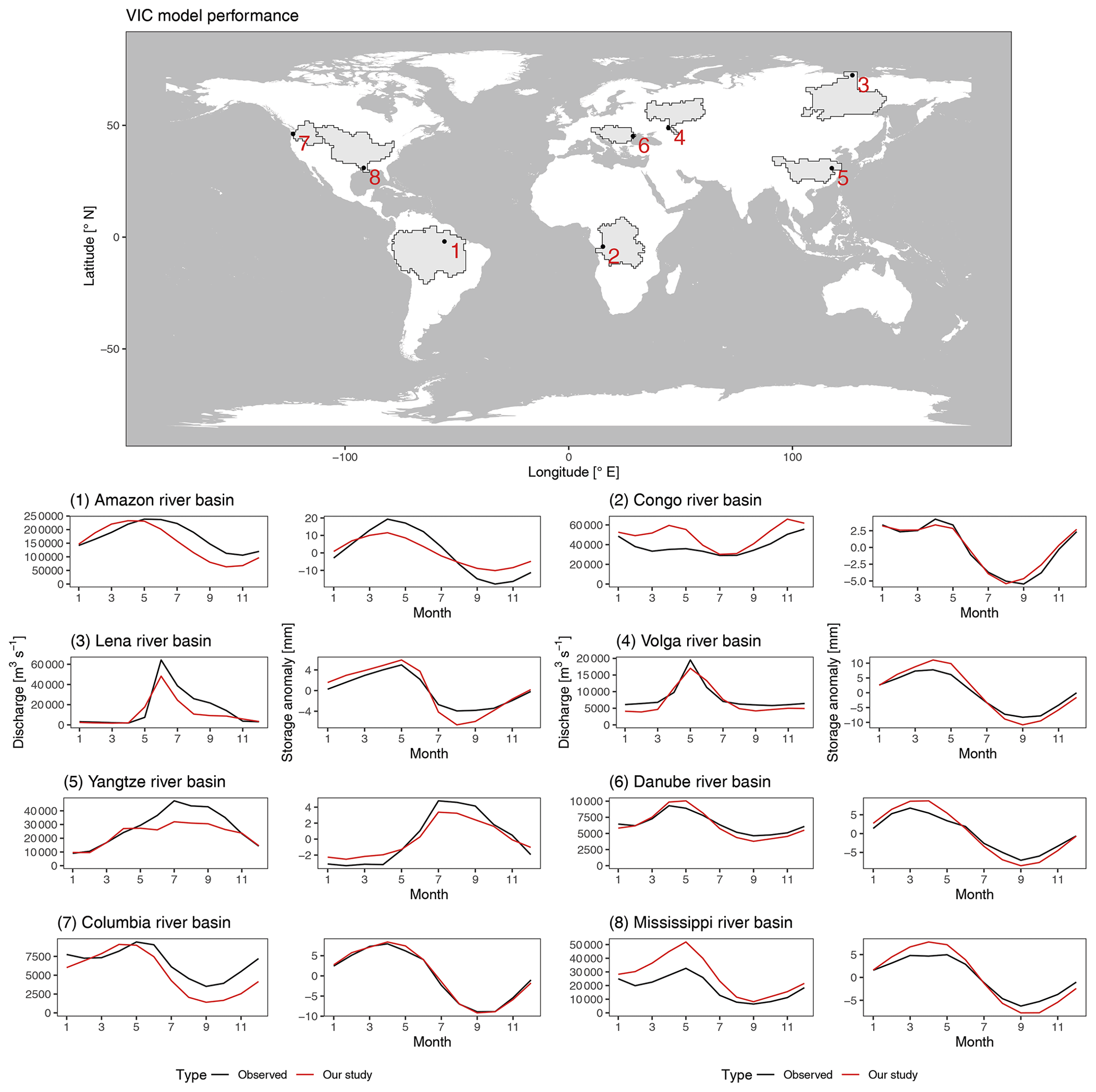
Figure E1 Comparison between simulated discharge and terrestrial total water storage anomalies and GRDC- and GRACE-observed values. Panels indicate the multiyear averages of anthropogenically impacted simulations (red) and observations (black).