The Ensemble Framework For Flash Flood Forecasting (EF5) v1.2: description and case study

The Ensemble Framework For Flash Flood Forecasting (EF5) was developed specifically for improving hydrologic predictions to aid in the issuance of flash flood warnings by the US National Weather Service. EF5 features multiple water balance models and two routing schemes which can be used to generate ensemble forecasts of streamflow, streamflow normalized by upstream basin area (i.e., unit streamflow), and soil saturation. EF5 is designed to utilize high-resolution precipitation forcing datasets now available in real time. A study on flash-flood-scale basins was conducted over the conterminous United States using gauged basins with catchment areas less than 1000 km². The results of the study show that the three uncalibrated water balance models linked to kinematic wave routing are skillful in simulating streamflow.

1 Introduction

Flash floods are defined by an extreme flow into a normally dry area or a rapid water level rise above a threshold flood level. Typically, flash flood events begin within minutes to a few hours after the causative rainfall event, although the timing can vary in different parts of the world (NWS, 2016; WMO, 1988). An upper bound for the drainage area of basins is often considered as 1000 km² (AMS, 2000). This definition of flash flooding also defines the requirements for any distributed hydrologic modeling system designed to forecast them. Such a system must be capable of cycling sub-hourly while providing forecasts for at least 6 h in the future. The system also must be able to resolve drainages with basin areas less than 1000 km².

In the United States, floods and flash floods are the second-deadliest weather phenomena behind heat (Ashley and Ashley, 2008). Flash flood fatalities have previously been found to account for 80–90 % of all flood fatalities. Globally, WMO (2008) found that there are currently 99 countries which issue flash flood warnings, but with 91 countries stating that further improvements to the warnings are necessary. The American Meteorological Society (AMS) policy statement on flash floods states, “forecasting the time and location of flash floods requires high-resolution modeling of weather and water, assimilation of large data sets from high-resolution observations, and an integrated, coherent approach that allows meteorologists and hydrologists to make rapid assessments and warning decisions” (AMS, 2017). Improved radar rainfall estimates are now available at 1 km² and 2 min spatiotemporal resolution, driving the demand for hydrologic forecasting systems which are capable of matching this resolution. This study will detail the development of a new high-resolution distributed hydrologic modeling framework which is capable of producing 0 to 24 h forecasts of streamflow, unit streamflow, and soil saturation while ingesting high-resolution radar rainfall estimates with a 10 min update cycle across continental scales. The goal of this framework is to be able to rapidly produce hydrologic assessments of flash flooding that guide operational warning decisions.

This study is part of the larger Flooded Locations And Simulated Hydrographs (FLASH) project, which aims to provide National Weather Service (NWS) forecasters with better warning decision support tools for issuing flash flood warnings in the United States (Gourley et al., 2017). Specifically the goal of the project is to improve the spatial specificity, timing, and accuracy of flash flood warnings by leveraging Multi-Radar Multi-Sensor (MRMS) rainfall products for high-resolution hydrologic forecasting. This study documents the hydrologic models used for FLASH, their setup, and their performance over the current period of record for the available high-resolution precipitation forcing. These hydrologic models have already been used for experimental evaluations with NWS forecasters in the Hydrometeorological Testbed (HMT-Hydro) (Martinaitis et al., 2017) and the Flash Flood and Intense Rainfall (FFaIR) experiments (Barthold et al., 2015). In both experiments, the hydrologic products presented here received favorable reviews. These hydrologic products have been used for experiments with automation in the warning decision process by recommending locations for possible flash flood warnings (Argyle et al., 2017). This paper will provide a review of existing hydrologic models, document the hydrologic models used in EF5, and demonstrate the performance of the hydrologic simulations with a multi-year case study over the United States.

Review of existing hydrologic models

Resolving extreme rainfall and flash flood events requires radar rainfall estimates coupled with distributed hydrologic models that need to be run at fine spatial resolution on the order of 100 m to 2 km with a temporal step that is sub-hourly (Rafieeinasab et al., 2015). With this requirement, several distributed hydrologic models were evaluated for their potential to be run in this fashion to capture flash flood events over the conterminous United States (CONUS). Given the focus on extreme rainfall events where contributions of surface fluxes into the atmosphere are small compared to the magnitude of the rainfall, it is sufficient to examine models with one-way coupling of rainfall onto the land surface. The Two-dimensional, Runoff, Erosion, and Export (TREX) distributed hydrologic model was one option; however the model attempts to be fully physical, meaning that it requires very fine spatial resolution and time steps on the order of seconds in order to properly solve the equations (Velleux et al., 2008). Running it over the CONUS would require computational resources unavailable at the present time for flash flood forecasting. Since a fully physically based distributed hydrologic model is too computationally complex to run with the required cycling times, there is a need to identify the trade-off required to run conceptually based hydrologic models. A brief literature review follows to answer the question, how accurate are the physically based hydrologic models and can we produce equal forecasts and understanding with a conceptually simpler model?

Devia et al. (2015) provides an overview of the differences between empirical (statistical), conceptual (parametric), and fully physical hydrologic models. The authors provide valuable dialog recognizing that each formulation of a hydrologic model has strengths and weaknesses and there is no one answer for the entire problem domain in hydrology right now. Empirical models are considered to be useful only for the specific watershed they are developed on and cannot be trivially extended into new watersheds. Empirical models also perform poorly for extreme events that occur outside of their training datasets. Conceptual models are defined as simple and easy to implement in software but require large amounts of data for calibration. Physically based models require extensive amounts of data on processes often not observed by current sensor networks and suffer from an inability to scale to large collections of watersheds. They further state that “Each model has various drawbacks like lack of user friendliness, large data requirements, absence of clear statements of their limitations etc. In order to overcome these defects, it is necessary for the models to include rapid advances in remote sensing technologies, risk analysis, etc. By the application of new technologies, new distributed models can be developed for modeling gauged and ungauged basins.” This belief is also held by the authors of this study, which leads to the creation of EF5.

Beven et al. (2014) addresses the ever-increasing spatiotemporal resolutions of hydrologic models and particularly the land surface models coupled to atmospheric weather prediction models. They argue that there is a lack of information available to validate hypotheses made in hyper-resolution models, which may lead to mistaken beliefs about the processes. Information from hyper-resolution models is often presented to stakeholders but without adequate quantification of the uncertainty, leading to precise but inaccurate forecasts. Further, the information is presented where only part of the model is hyper resolution and, for example, the precipitation forcing may not support the ability to resolve details at the resolutions being presented on maps. Kuczera et al. (2010) address the problem of uncertainty in the forcing information used for hydrologic models and model structural error. They argue that because of uncertainties in the forcing information, averaging methods applied to obtain it, and hydrologic model structural error, no conceptual model should be presented in a deterministic way. The argument about model structural error suggests that future modeling systems should be able to account for these uncertainties with different model structures. Micovic and Quick (2009) look at the complexity of model representation needed as the temporal resolution of the hydrologic model decreases. So as simulations move from long-term climate simulations at a daily time step to simulations for individual days with extreme flood events, is there a need for more hydrologic model complexity? The results from the study are only valid over a single watershed but suggest that important hydrologic processes for extreme flooding are different than the processes yielding good prediction skill at long time ranges.

More recently, the US NWS implemented the National Water Model (NWM), which is a variant of the Weather Research and Forecasting Model Hydrological modeling system (WRF-Hydro) (Gochis et al., 2014). This modeling framework is more holistic in that it is being developed to address multiple hydrologic applications, including water resources management, stream temperature forecasting, coupling to storm surge models for coastal flooding applications, surface and groundwater interactions, and channel losses in semi-arid environments. The wide range of applications requires more model complexity, and thus the framework utilizes the Noah-Multiparameterization land surface model (NOAH-MP) as its core. The utility of the NWM for flash flood forecasting will require sub-hourly data latency, yet there has been some recent progress on applications (Viterbo et al., 2020).

Given the evidence above, the choice of a hydrologic model for CONUS-wide flash flood prediction seems to fall to multiple conceptual models which are computationally efficient. The Coupled Routing and Excess Storage (CREST) distributed hydrologic model developed by Wang et al. (2011) was picked for initial inclusion into the modeling framework because of its use previously at the global scale. The Sacramento Soil Moisture Accounting model (SAC-SMA), in a distributed fashion similar to the Hydrology Laboratory Research Distributed Hydrologic Model (HL-RDHM), was also picked for inclusion in the framework because of its existing operational use by the US National Weather Service (Koren et al., 2004; Burnash, 1995). Existing implementations of both water balance schemes were tied to specific projects with details that precluded the easy use with forcing at a 1 km² and 2 min resolution, necessitating new implementations in more flexible tools.

2 Ensemble Framework For Flash Flood Forecasting (EF5)

2.1 Introduction

The ideas behind EF5 were to incorporate the CREST water balance model and SAC-SMA water balance model and then have the runoff output from either of those force a river routing scheme. Kinematic and linear reservoir wave routing were the first river routing schemes implemented because of their overall computational efficiency. Applying EF5 at different locations made it apparent that there was a need for snow parameterization, so the Snow Accumulation and Ablation model (Snow-17) (Anderson, 1976) was added to EF5. Additionally it was identified that for some use cases calibration of the hydrologic models was desirable, so the Differential Evolution Adaptive Metropolis (DREAM) automatic calibration scheme (Vrugt et al., 2009) was incorporated into EF5. EF5 also has limited data assimilation capabilities supporting only direct insertion, which can also be used as a boundary condition to model a smaller area of a large watershed (Houser et al., 2012). Figure 1 is the flow chart for EF5 showing the various models and options that can be utilized for distributed hydrologic modeling with a focus on flash flooding.

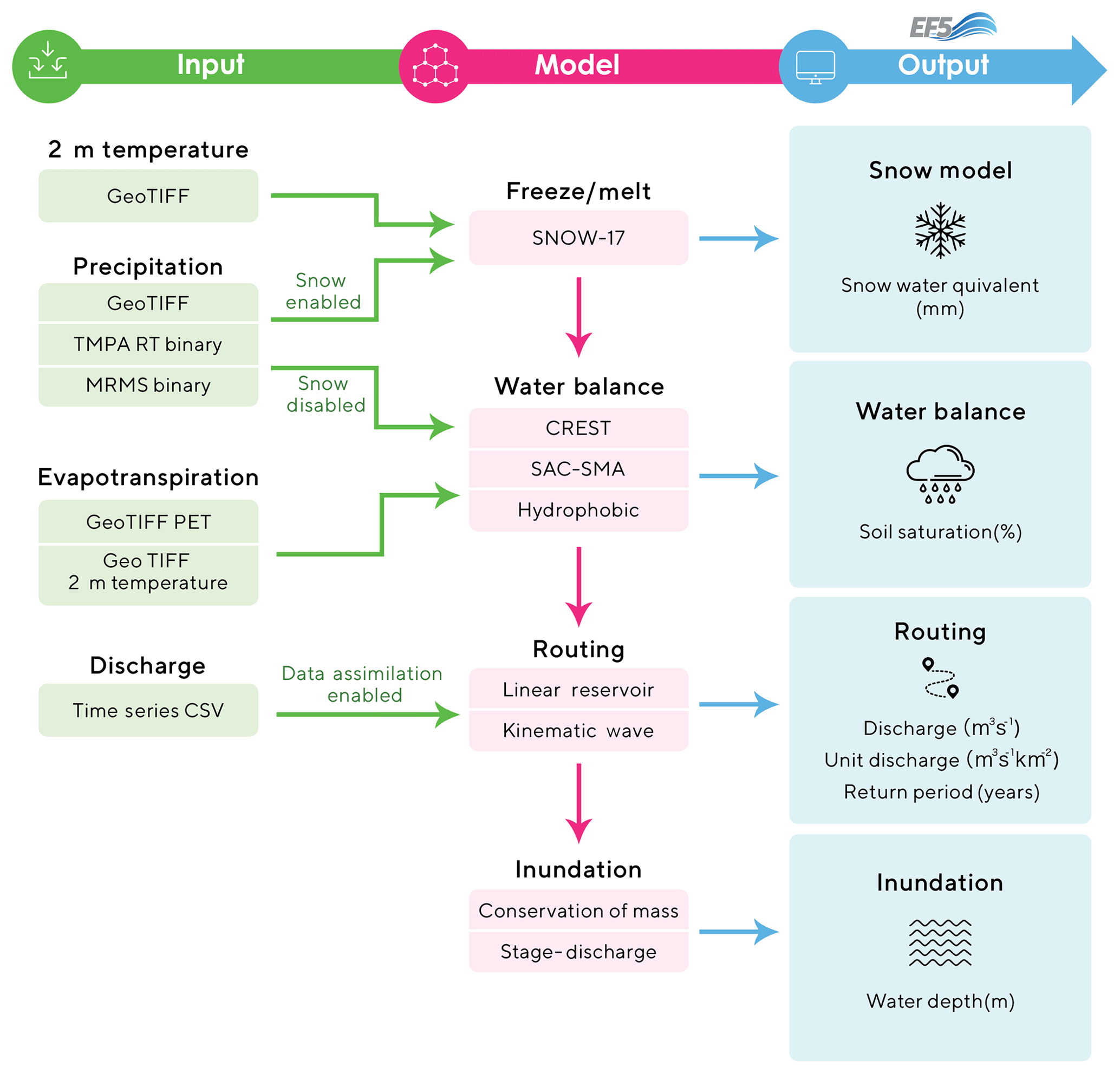
Figure 1 Flow chart illustrating the different modules and options available in EF5. The arrows show the paths available for input data to flow between the modules. The modules can be enabled or disabled from the control file to get the desired final model configuration.

To pick an area to model the basic files must first be provided, which include digital elevation map (DEM), flow direction map (FDM), and flow accumulation map (FAM). EF5 is resolution independent and will work with any DEM resolution having been tested from 0.5 m to 12 km. Note that the a priori parameters for the water balance models were derived at 1 km and will need to be resampled to the DEM grid cell resolution. While the overland parameters are linked to observable features of the land surface and soil properties, there can still be a scale dependence of model results due to DEM resolution differences. Finer-scale DEMs are capable of resolving more details of the terrain such as steeper slopes in mountainous areas. This can cause the model to produce higher and faster peak flows when going to finer-scale DEMs. Furthermore, the routing parameters are scale dependent and will need to be re-derived for resolutions other than 1 km (additional details provided in Sect. 2.3.2). Links to the parameter grids are provided in the code availability section at the close of the paper. The downstream point to model is then identified as a “gauge”, which may or may not also correspond to an observation measurement location. Groups of gauges can be collected into a “basin”, which is fundamentally just a collection of gauges one wishes to model on and not necessarily a collection of gauges in the same physical watershed. Parameters for the models are specified on a per-gauge basis and then applied everywhere upstream of the gauge as a multiplier onto the distributed values until the next gauge if there is one. The parameters are specified either as a distributed grid and then a multiplier value or as a single value that is applied uniformly across the watershed.

EF5 is written in C++ and currently contains 20 388 lines of code while supporting Linux, Mac OS X, and Windows operating systems. Linux and Mac OS X are supported via binaries run from the shell command prompt, while Windows features a fully fledged graphical user interface (GUI). The Windows GUI provides very similar visual feedback when compared to the Linux and Mac OS X versions but in an easier-to-work-with package.

EF5 currently supports several different options for file formats and map projections. The preferred file format for use with EF5 is Geographic Tagged Image File Format (GeoTIFF), which has the distinct advantage of including native compression capabilities, reducing file sizes greatly. Environmental Systems Research Institute (ESRI) Arc ASCII grids are also supported as input options for all gridded fields. For precipitation input, MRMS binary, the Tropical Rainfall Measuring Mission (TRMM) Multisatellite Precipitation Analysis (TMPA) 3B42 real-time binary are all supported input options.

EF5 was created in a modular way to support multiple model physics, and to do so implements virtual base classes for the snow melt, water balance, and routing physics. The water balance base class is detailed below, and thus it is possible for any water balance model that can conform to this specification to be implemented into EF5. EF5 provides two input forcing variables for the water balance component, precipitation and potential evapotranspiration. The output variables are a fast-flow (typically surface) component, slow-flow (typically subsurface) component, and a soil saturation value.

The base class contains methods for initializing the model, initializing model state variables that may have been saved to file, saving model state variables to file, and finally performing the water balance physics itself. The routing and snow components contain similar methods to be implemented to those in the water balance component, with functionality for initialization, state loading and saving, and the main method for executing the physics. The routing virtual class takes fast-flow and slow-flow input components and provides a single discharge output variable. The snow module takes as input precipitation and temperature, while providing melted runoff (or just passing through precipitation in the no-snow case) and snow water equivalent as the output variables.

This implementation of the model physics allows for EF5 to be easily expanded in the future to contain more options for treatment of basic hydrologic functions. This expandability is an important feature because it provides a way for new physics to be added to existing operational flood forecasting systems in the future without a complete overhaul of the supporting infrastructure.

2.2 Water balance models

Currently EF5 contains three water balance options. All three options are conceptually based and rely on parameters guided by land surface and subsurface properties measured in existing data sources. The three options described in this section are CREST, SAC-SMA, and a hydrophobic (HP) model. The most detailed description is provided for the CREST model because the underlying model has been modified from previous publications (Wang et al., 2011).

2.2.1 Hydrophobic (HP)

The HP option is by far the simplest, as there are no parameters to be specified for the land surface. The HP option treats the surface as completely impervious, so all rain immediately runs off and flows downslope. The HP water balance option is included for the ability to diagnose processes and errors when running in an ensemble with the other water balance models. Underestimation of streamflow with the HP model indicates that the precipitation is likely biased. The HP model produces an upper bound on the expected discharge values. If the hydrophobic solution matches closely with the observed streamflow, then either the entire drainage area is acting as an impervious surface or the inputs into the model are underestimating the magnitude of rainfall.

Given that the hydrophobic model provides the “worst-case scenario” in terms of runoff responses to rainfall, operational forecasters have used it to approximate hydrophobic land surfaces for situations in which the soils were completely saturated, for urbanized basins that allowed very little infiltration, and for soils that had been affected by wildfire. Running EF5 in an ensemble with all three water balance models allows for the impacts of wildfires to be considered without having to modify distributed model parameter grids. This allows for quicker operational response to changing land surface conditions in the event of a wildfire that is followed immediately by heavy-rainfall events.

2.2.2 Coupled Routing and Excess Storage (CREST)

Another water balance option, CREST, is a derivative of the Xinanjiang model developed for use in China which features a variable infiltration curve for partitioning rainfall into direct runoff and infiltration (Ren-Jun, 1992; Liang et al., 1996; Liu et al., 2009). Wang et al. (2011) documented the first version of CREST, and the version used here is an adaptation of that. The EF5/CREST implementation has only a single soil layer, further simplifying the model and reducing the input data requirements. EF5/CREST also contains partitioning for impervious area. Figure 2 shows a schematic for the various processes represented in EF5/CREST to convert rainfall into runoff.

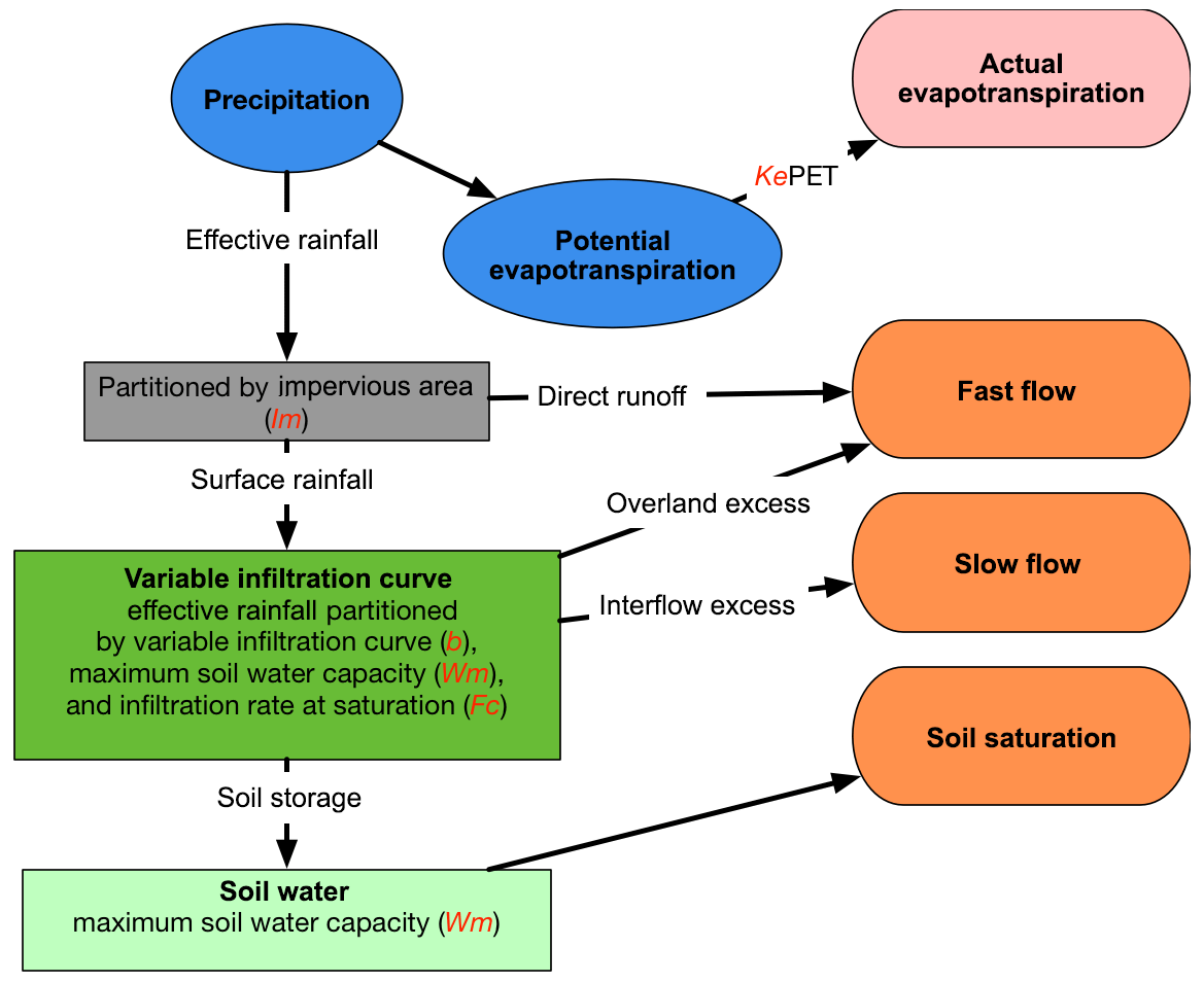
Figure 2 A schematic showing the progression of processes represented in the EF5/CREST water balance component.

Since EF5/CREST differs significantly from previous versions of CREST, a detailed description of EF5/CREST is provided here. The first step is converting potential evapotranspiration to effective evapotranspiration using the configurable scalar parameter K_e as shown in Eq. (1). The K_e parameter is typically set to 1.0 when working with distributed potential evapotranspiration and not utilizing model calibration.

$$\begin{array}{}\text{(1)}& {\text{EET}}_t=K_{\mathrm{e}}\cdot {\text{PET}}_t\end{array}$$

PET_t is potential evapotranspiration input forcing data into EF5, and EET_t is the effective evapotranspiration. PET_t in EF5/CREST is often computed using the Penman–Monteith equation (Montieth, 1965), which computes the potential evapotranspiration as a function of air temperature. Climatologies of air temperature can then be used to compute monthly mean or even hourly PET for use with EF5.

$$\begin{array}{}\text{(2)}& {\text{EP}}_t=\left\{\begin{array}{ll}\mathrm{0},& \text{for}{\text{EET}}_t\ge P_t\\ P_t-{\text{EET}}_t,& \text{for}{\text{EET}}_t<P_t\end{array}\right.\end{array}$$

P_t is the input forcing rainfall into EF5. From the effective rainfall (EP_t) the direct runoff portion is calculated, with the rest falling to the soil and then the infiltration process. The rainfall is then partitioned into a portion reaching the soil (SP_t), a portion contributing to actual ET, and a portion contributing to direct runoff (DP_t).

$$\begin{array}{}\text{(3)}& {\displaystyle }{\text{DP}}_t={\text{EP}}_t\cdot I_m\text{(4)}& {\displaystyle }{\text{SP}}_t={\text{EP}}_t\cdot (\mathrm{1}-I_m)\end{array}$$

I_m is a scalar parameter representing the percent impervious area. One way the I_m parameter is derived is using satellite-based land use and land cover (LULC) maps, which denote cities where land has been transformed into impermeable surfaces through human activity. The satellite LULC maps are typically at a very fine resolution, which can then be averaged to the coarser resolution of the model thus providing the percentage of impervious area per grid cell. The infiltration is then modeled using

$$\begin{array}{}\text{(5)}& I_t=\left\{\begin{array}{l}\mathrm{0},\\ \text{for}{P}_t\le {\text{EET}}_t\vee {\text{SM}}_t\ge W_{\mathrm{m}}\\ W_{\mathrm{m}}-{\text{SM}}_t,\\ \text{for}(i_t+{\text{SP}}_t)\ge I_m\\ W_{\mathrm{m}}-{\text{SM}}_t-W_{\mathrm{m}}\cdot [\mathrm{1}-\frac{i_t+{\text{SP}}_t}{i_{\mathrm{m}}}{]}^{\mathrm{1}+b},\\ \text{for}(i_t+{\text{SP}}_t)<I_m\end{array}\right..\end{array}$$

W_m represents the maximum water capacity, SM_t is the soil moisture state variable, and b represents the exponent of the variable infiltration curve. Both W_m and b are parameters in EF5/CREST that are configurable but often defined a priori . i_m represents the maximum infiltration capacity defined by

$$\begin{array}{}\text{(6)}& i_{\mathrm{m}}=W_{\mathrm{m}}\cdot (\mathrm{1}+b).\end{array}$$

The infiltration capacity at the current time, i_t, is defined as

$$\begin{array}{}\text{(7)}& i_t=i_{\mathrm{m}}\cdot \left[\mathrm{1}-{\left(\mathrm{1}-{\displaystyle \frac{{\text{SM}}_t}{W_{\mathrm{m}}}}\right)}^{\frac{\mathrm{1}}{\mathrm{1}+b}}\right].\end{array}$$

The effective precipitation is then partitioned into excess rainfall (ER_t) based on the infiltration.

$$\begin{array}{}\text{(8)}& {\text{ER}}_t=\left\{\begin{array}{ll}\mathrm{0},& \text{for}{\text{SP}}_t=\mathrm{0}\vee {\text{SP}}_t\le I_t\\ {\text{SP}}_t-I_t,& \text{for}{\text{SP}}_t>I_t\end{array}\right.\end{array}$$

The excess rainfall is then divided into overland (OER_t) and subsurface (SER_t) flow components by

$$\begin{array}{}\text{(9)}& {\text{SER}}_t=\left\{\begin{array}{ll}\mathrm{0},& \text{for}{\text{EP}}_t=\mathrm{0}\\ {\text{temX}}_t,& \text{for}{\text{ER}}_t>{\text{temX}}_t\\ {\text{ER}}_t,& \text{for}{\text{ER}}_t\le {\text{temX}}_t\end{array}\right.,\end{array}$$

with temX_t defined as

$$\begin{array}{}\text{(10)}& {\text{temX}}_t=\left\{\begin{array}{ll}\frac{{\text{SM}}_t+W_t}{\mathrm{2}{W}_{\mathrm{m}}}\cdot F_{\mathrm{c}},& \text{for}{\text{EP}}_t>\mathrm{0}\\ ({\text{EET}}_t-P_t)\cdot \frac{{\text{SM}}_t}{W_{\mathrm{m}}},& \text{for}{\text{EP}}_t=\mathrm{0}\end{array}\right.,\end{array}$$

using F_c to represent the hydraulic conductivity and with W_t as

$$\begin{array}{}\text{(11)}& W_t=\left\{\begin{array}{ll}\mathrm{0},& \text{for}{\text{EP}}_t=\mathrm{0}\\ W_{\mathrm{m}},& \text{for}{\text{SM}}_t+I_t\ge W_{\mathrm{m}}\\ {\text{SM}}_t+I_t,& \text{for}{\text{SM}}_t+I_t<W_{\mathrm{m}}\end{array}\right..\end{array}$$

The overland flow component is then calculated by taking a difference between the amount that infiltrates and the excess rain plus adding in the direct runoff.

$$\begin{array}{}\text{(12)}& {\text{OER}}_t=\left\{\begin{array}{ll}\mathrm{0},& \text{for}{\text{EP}}_t=\mathrm{0}\\ {\text{ER}}_t-{\text{SER}}_t+{\text{DP}}_t,& \text{for}{\text{EP}}_t>\mathrm{0}\end{array}\right.\end{array}$$

The new soil moisture value is then computed using

$$\begin{array}{}\text{(13)}& {\text{SM}}_{t+\mathrm{1}}=\left\{\begin{array}{ll}{\text{SM}}_t-{\text{temX}}_t,& \text{for}{\text{EP}}_t=\mathrm{0}\\ W_t,& \text{for}{\text{EP}}_t>\mathrm{0}\end{array}\right..\end{array}$$

Finally the actual evapotranspiration, AET_t, is given as

$$\begin{array}{}\text{(14)}& {\text{AET}}_t=\left\{\begin{array}{ll}{\text{temX}}_t& \text{for}{\text{EP}}_t=\mathrm{0}\\ {\text{EET}}_t,& \text{for}{\text{EP}}_t>\mathrm{0}\end{array}\right..\end{array}$$

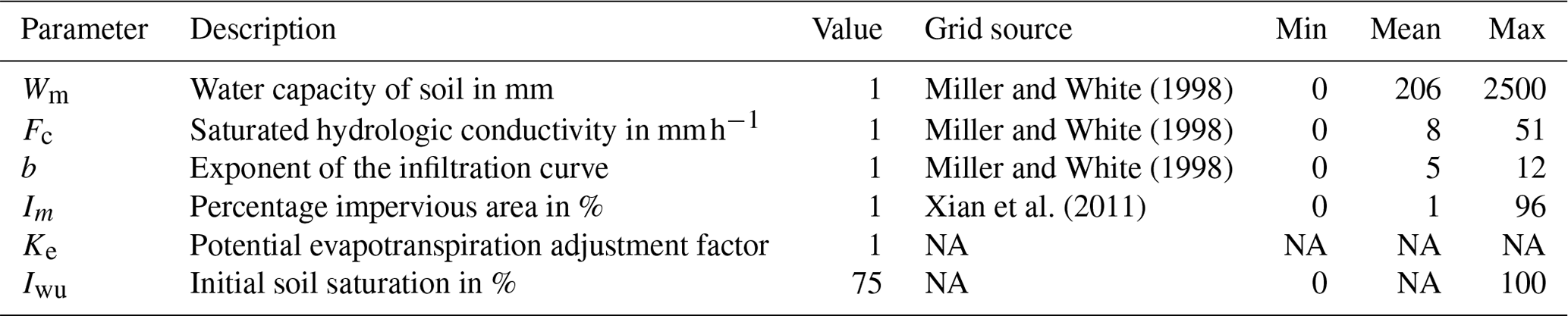
EF5/CREST has six configurable parameters. W_m is the cell's maximum water capacity and is closely related to the soil porosity over the first 50 to 100 cm of soil. This parameter controls how much water is necessary for a grid cell to become saturated and can be viewed as a bucket that fills up. F_c is the maximum amount of water allowed to infiltrate into the subsurface flow when the grid cell is saturated. This parameter is closely related to saturated hydraulic conductivity. K_e is a linear adjustment to potential evapotranspiration and controls how efficiently potential evapotranspiration is converted into actual evapotranspiration. The b parameter is related to the soil texture. I_m is the percent of rain that is converted directly into overland runoff. This parameter is related to the impervious area of the grid cell. The final parameter, I_wu is the percent of W_m that is water initially in the grid cell. This is really a model state, but to allow for more thorough model calibration it is classified as a parameter value. Section 3.1 describes typical sources and gives examples of the EF5/CREST parameters described in this section.

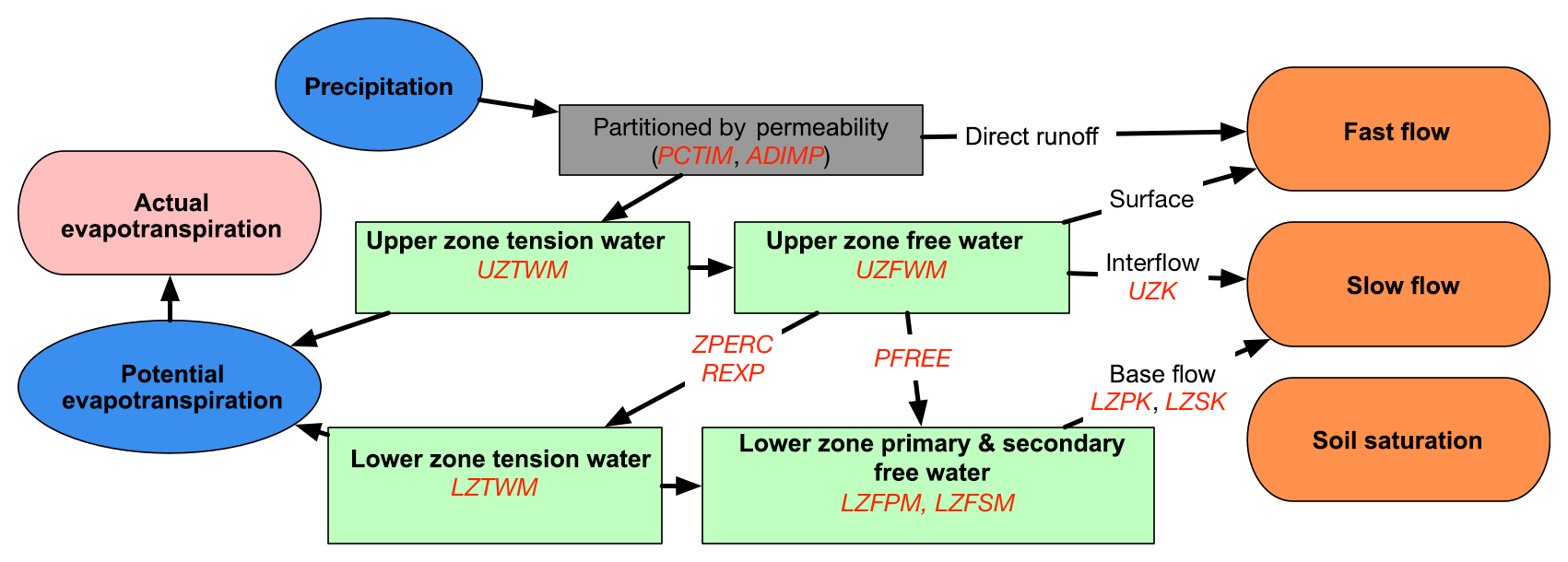
Figure 3 A schematic showing the progression of processes, inputs, and outputs represented in the EF5/SAC-SMA water balance component.

2.2.3 Sacramento Soil Moisture Accounting (SAC-SMA)

The SAC-SMA water balance option is the most complex one featured in EF5 currently. The implementation of SAC-SMA in EF5 is based off the works of Koren et al. (2004) and Yilmaz et al. (2008), so the model structural details are not described here. Figure 3 is a schematic of the processes represented in the SAC-SMA water balance component. Multiple zones with significantly more complex interactions are included in SAC-SMA as compared with EF5/CREST. The 21 parameters for EF5/SAC-SMA are listed and briefly described in Table 3. The SAC-SMA uses a saturation excess process to generate runoff differing from the infiltration excess process used in EF5/CREST. Like EF5/CREST the Sacramento model utilizes a partition of rainfall between impervious and permeable surfaces, with impervious area contributing directly to runoff in a grid cell.

The EF5/SAC-SMA water balance model features an upper and lower layer (zone), which absorb and transmit water in conceptually different ways. The upper zone acts as the short-term storage capacity for the grid cell, so it is the first to fill when rainfall occurs. The lower zone serves to provide the baseflow and acts as the long-term storage capacity for the grid cell. Each zone is further subdivided into tension water and free water. Tension water acts as surface tension and can only be removed from the grid cell by evapotranspiration. Free water can move through the cell vertically to the lower zone from the upper zone or be discharged as streamflow out of the grid cell.

2.3 Routing options

2.3.1 Linear reservoir

The routing options available in EF5 are a lumped routing model conceptualized as a series of linear reservoirs and a kinematic wave (KW) approximation of the Saint-Venant equations for one-dimensional open-channel flow. The linear reservoir option is adapted from the original CREST model (Wang et al., 2011) and has been well described and used in many hydrologic projects (Nash, 1957; Moore, 1985; Chow et al., 1988; Vrugt et al., 2002). The EF5 linear reservoir option features two separate reservoirs, where their depths are computed as

$$\begin{array}{}\text{(15)}& {\displaystyle }{\text{OR}}_{t+\mathrm{1}}={\text{OR}}_t+{\text{OER}}_t+\sum _{i=\mathrm{1}}^N{\text{OER}}_t^i,\text{(16)}& {\displaystyle }{\text{SR}}_{t+\mathrm{1}}={\text{SR}}_t+{\text{SER}}_t+\sum _{i=\mathrm{1}}^N{\text{SER}}_t^i,\end{array}$$

where OR_t and SR_t are the overland and subsurface reservoirs, respectively. OER_t and SER_t are the excess rainfall components from EF5/CREST, representing the fast- and slow-flow components, respectively. The N represents the number of adjacent grid cells that flow into the current grid cell. The discharge out of each reservoir is based on the linear equations

$$\begin{array}{}\text{(17)}& {\displaystyle }{\text{OQ}}_{\mathrm{t}}=\text{LeakO}\cdot {\text{OR}}_t,\text{(18)}& {\displaystyle }{\text{SQ}}_{\mathrm{t}}=\text{LeakI}\cdot {\text{SR}}_t,\text{(19)}& {\displaystyle }{Q}_{\mathrm{t}}={\text{OQ}}_{\mathrm{t}}+{\text{SQ}}_{\mathrm{t}}.\end{array}$$

LeakO and LeakI are parameters defining the rate of discharge. The total discharge Q_t is based on the summation of the fast (OQ_t) and slow (SQ_t) discharge rates. At each time step the fast and slow discharges are routed downstream following the FDM into the reservoir of the downstream grid cell.

2.3.2 Kinematic wave

The implementation of the kinematic wave routing is based on an approximation to the one-dimensional unsteady open-channel flow equations. The full one-dimensional unsteady open-channel flow equations were developed in 1871 by Barré de Saint-Venant and represent a physical description of the movement of water in a watershed (Chow et al., 1988). The full equations have a number of assumptions that must be met, including that the flow is one-dimensional; the flow varies gradually along the channel, implying vertical accelerations can be neglected; the channel is approximately a straight line within a given grid cell; the channel does not experience scour or deposition; and the flow fluid is incompressible, implying a constant density. The kinematic wave model further simplifies the equations and requires that the bed slopes are steep. In the steep-slope case the kinematic wave approximation reasonably describes the unsteady flow phenomena (Ponce, 1986). The work by Ponce (1991) claims that even in most overland cases the criteria for the kinematic wave approximation hold. The kinematic wave model is widely used in hydrology and has been implemented in systems such as the Hydrologic Engineering Center's Hydrologic Modeling System (Feldman, 2000), the Storm Water Management Model created by the Environmental Protection Agency (Huber, 1995), HL-RDHM previously mentioned here and described in Koren et al. (2004), and finally already coupled to the Xinanjiang model (Liu et al., 2009).

Deriving the kinematic wave approximation starts with the Saint-Venant equations in the Eulerian frame of reference, where we model fluid as it passes by a control point, or in this case as it passes through a control volume. The time rate of change of the fluid is modeled as a function of the external forces acting on it as in the Reynolds transport theorem (Chow et al., 1988). The external forces in this case are derived from Newton's second law of motion while neglecting lateral inflow, eddies, and wind shear. The Saint-Venant continuity equation is given as

$$\begin{array}{}\text{(20)}& {\displaystyle \frac{\partial Q}{\partial x}}+{\displaystyle \frac{\partial A}{\partial t}}=q,\end{array}$$

where Q is the discharge, x is the horizontal distance, q is the lateral inflow into the channel, t is time, and the channel cross-sectional area is A. The equation of momentum is defined by

$$\begin{array}{}\text{(21)}& {\displaystyle \frac{\mathrm{1}}{A}}{\displaystyle \frac{\partial Q}{\partial t}}+{\displaystyle \frac{\mathrm{1}}{A}}{\displaystyle \frac{\partial }{\partial x}}\left({\displaystyle \frac{Q^{\mathrm{2}}}{A}}\right)+g{\displaystyle \frac{\partial y}{\partial x}}-g{S}_{\mathrm{o}}+g{S}_{\mathrm{f}}=\mathrm{0},\end{array}$$

where gravity is g, S_o is the bottom channel slope, and S_f is the friction slope. The terms in Eq. (21) have been named such that $\frac{\mathrm{1}}{A}\frac{\partial Q}{\partial t}$ is the local acceleration, $\frac{\mathrm{1}}{A}\frac{\partial }{\partial x}\left(\frac{Q^{\mathrm{2}}}{A}\right)$ is the convective acceleration, $g\frac{\partial y}{\partial x}$ is the pressure force, gS_o is the gravity force, and gS_f is the friction force. Simplifications to Eqs. (20) and (21) represent different schemes commonly used in distributed hydrologic models. When no simplifications are made, the routing is referred to as dynamic wave; when the acceleration terms are neglected, the resulting wave model is called diffusive wave; and when the acceleration terms are neglected and the gravity force and friction force are assumed to be equal, the result is the kinematic wave routing. In the kinematic wave assumption the resulting equation for momentum is

$$\begin{array}{}\text{(22)}& Q=\mathit{\alpha }{A}^{\mathit{\beta }},\end{array}$$

where α and β are the KW parameters. This can be substituted back into the continuity equation and solved for Q, which yields

$$\begin{array}{}\text{(23)}& {\displaystyle \frac{\partial Q}{\partial x}}+\mathit{\alpha }\mathit{\beta }{Q}^{\mathit{\beta }-\mathrm{1}}{\displaystyle \frac{\partial Q}{\partial t}}=q.\end{array}$$

Chow et al. (1988) also provides an implicit solution to the equations for distributed routing which is implemented in EF5. The kinematic wave routing in EF5 is applied only to the overland discharge; the subsurface discharge is routed with linear reservoir routing as described above. The equations above describe the kinematic wave routing for channel routing. For overland routing the process is the same as above but for q instead of Q. The resulting equation is as follows:

$$\begin{array}{}\text{(24)}& {\displaystyle \frac{\partial q}{\partial x}}+{\mathit{\alpha }}_{\mathrm{0}}{\mathit{\beta }}_{\mathrm{0}}{q}^{{\mathit{\beta }}_{\mathrm{0}}-\mathrm{1}}{\displaystyle \frac{\partial q}{\partial t}}=i-f,\end{array}$$

where α₀ is the overland conveyance parameter, and the β₀ parameter is fixed at 3∕5. The i−f forcing term is the surface excess rainfall passed in from the water balance model. Table 4 details the parameter options for kinematic wave routing used by EF5.

3 Case study over the CONUS

3.1 EF5 setup

In November 2017, the initial operational version of EF5 was transitioned to the NWS. Due to limitations with operational computational resources, the initial operational version of EF5 consists of precipitation estimates coming from MRMS and serving all three water balance modules and has KW routing, but with no consideration of frozen-precipitation processes, no data assimilation, and no inundation mapping. The intention of this study is to evaluate the accuracy of the model version that was transitioned to the NWS as part of the EF5 initial operational capability. Future implementations will consider updates to model states, inclusion of Snow-17, and inundation mapping. The modeling domain was set to exactly match the MRMS domain over the CONUS with a regular 0.01^∘ grid spanning from −130.0 to −60.0^∘ longitude and 20.0 to 55.0^∘ latitude. This grid was picked to fully exploit the resolution provided by the MRMS precipitation estimates. The basic files – which are the digital elevation model (DEM), flow direction map (FDM), and flow accumulation map (FAM) – were derived from the US Geologic Survey (USGS) National Elevation Dataset (NED) (Gesch et al., 2009). The NED data were resampled to the 0.01^∘ resolution using an arithmetic mean, and then FDM and FAM were derived using ESRI ArcGIS and the ArcHydro toolbox. A priori distributed parameter maps are preferred where available and as such were used for impervious area and soil parameters in the hydrologic models. The models were run uncalibrated because there is a focus on providing information over the CONUS to improve flash flood warnings in overland areas which are not typically instrumented with gauges or adequately modeled through traditional regionalization approaches.

Miller and White (1998)Miller and White (1998)Miller and White (1998)Xian et al. (2011)

Table 1 Description of parameters used in the CREST water balance model.

NA: not available.

The CREST parameters used for this study are largely based on a priori maps of soil information generated by Miller and White (1998) utilizing the US Department of Agriculture State Soil Geographic (STATSGO) dataset. Table 1 summarizes the EF5/CREST parameters and the values used in this study. The b parameter was derived from the soil texture map provided by Miller and White (1998), with a lookup table from Cosby et al. (1984) then used to convert from the soil texture into the exponent parameter. The lookup table for b is provided in Table 2. The W_m parameter map was generated from resampling the available water capacity 250 cm depth map in Miller and White (1998) to the domain used here with bilinear interpolation. The F_c parameter for EF5/CREST was produced using the permeability map from Miller and White (1998). The percent impervious area was derived from the USGS National Land Cover Database (NLCD) 2011 edition impervious area from Xian et al. (2011) resampled using average interpolation onto the study domain. Figure 4 shows the spatial distributions of the non-uniform parameter values over the CONUS. The K_e and I_wu are the only EF5/CREST parameters without distributed a priori parameters.

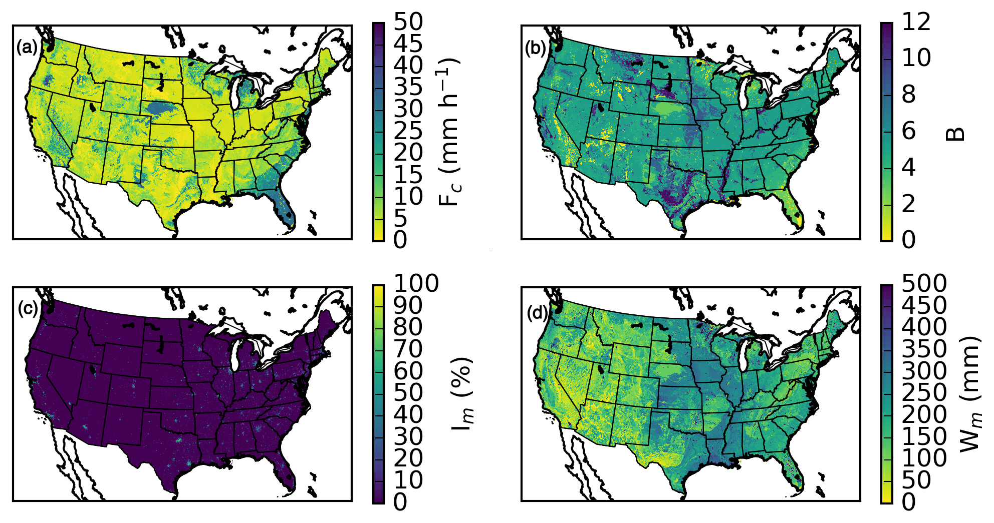
Figure 4 The EF5/CREST (a) F_c, (b) b, (c) I_m, and (d) W_m distributed parameters used in the study over the conterminous United States

The EF5/SAC-SMA parameters were taken directly from work done by Zhang et al. (2011) because this work is most comparable to what is used operationally by the NWS. Table 3 lists the parameters and their respective values used in this study. The PCTIM, ADIMP, SIDE, and RIVA parameters are using lumped values defined in the tables because a priori grids are not available.

Table 2 Soil texture and EF5/CREST b parameter value as derived from Cosby et al. (1984).

Zhang et al. (2011)Zhang et al. (2011)Zhang et al. (2011)Zhang et al. (2011)Zhang et al. (2011)Zhang et al. (2011)Zhang et al. (2011)Zhang et al. (2011)Zhang et al. (2011)Zhang et al. (2011)Zhang et al. (2011)

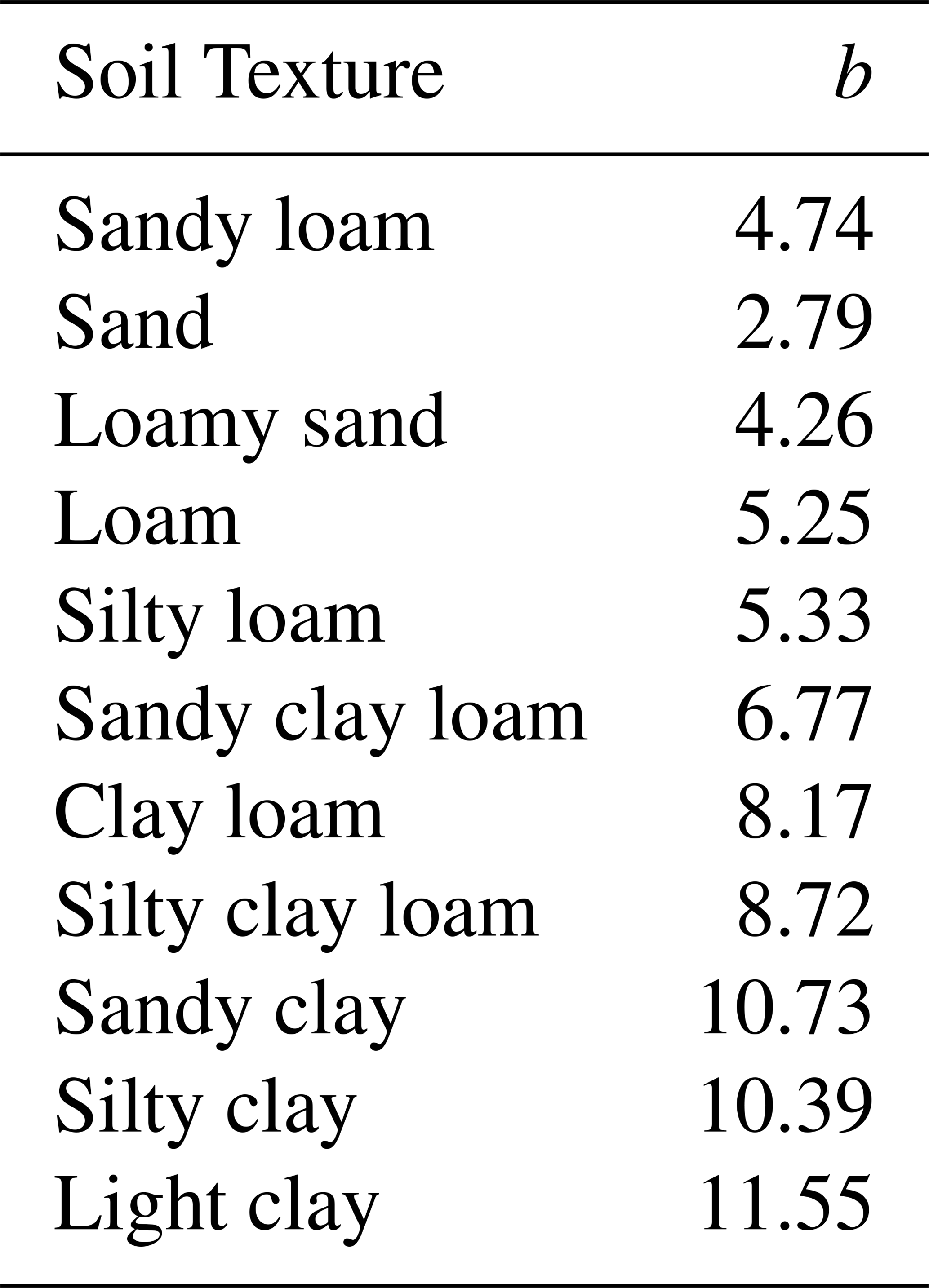
Table 3 Description of parameters used in the SAC-SMA water balance model.

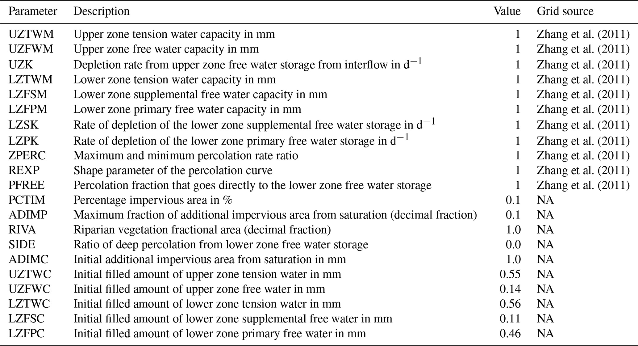
NA: not available.

The kinematic wave parameters used by EF5 are listed in Table 4. These parameter values are used for all model combinations when coupled with CREST, SAC-SMA, and HP water balance options for this study. The parameters are a priori based on statistical relationships with basin geomorphology, precipitation, and soil parameters developed in Vergara et al. (2016). Observed α and β values were computed from the cross sections, and discharge values measured by the USGS. These observed values were then modeled using Generalized Additive Models for Location, Scale, and Shape (GAMLSS; Rigby and Stasinopoulos, 2005), which allow for the extrapolation of information collected at the approximately 10 000 USGS discharge stations in the CONUS to everywhere on the hydrologic model grid. The parameters used are basin area, elongation ratio, relief ratio, slope index, local slope, mean annual precipitation, mean annual temperature, erodibility factor, depth to bedrock, rock volume percentage, soil texture, curve number, and river length.

Vergara et al. (2016)Vergara et al. (2016)Vergara et al. (2016)Miller and White (1998)Zhang et al. (2011)

Table 4 Description of parameters used in kinematic wave routing scheme.

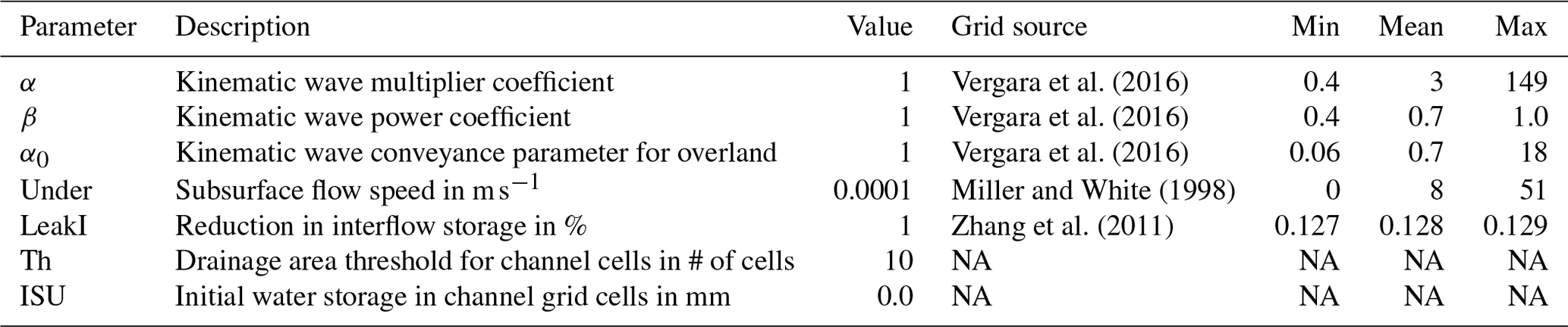
NA: not available.

Estimates for linear reservoir model parameters Under and LeakI for subsurface flow are based on F_c (hydraulic conductivity) and SAC-SMA's UZK parameter (Table 3), respectively, using conversion factors for unit consistency. The α₀ parameter was computed using Manning's equation for overland flow:

$$\begin{array}{}\text{(25)}& {\mathit{\alpha }}_{\mathrm{0}}={\displaystyle \frac{\mathrm{1}}{n}}{S}^{\frac{\mathrm{1}}{\mathrm{2}}},\end{array}$$

where the S is the slope computed from DEM and n is Manning's roughness coefficient. The roughness coefficient was computed from the University of Maryland (UMD) Moderate Resolution Imaging Spectroradiometer (MODIS) land cover type mosaics (Channan et al., 2014) and a lookup table from Chow et al. (1988) documented in Table 5. Figure 5 shows the resulting kinematic wave parameter maps for the CONUS. The parameters have clear signs of influence from the geophysical information used to derive them.

Table 5 Description of overland flow parameterizations.

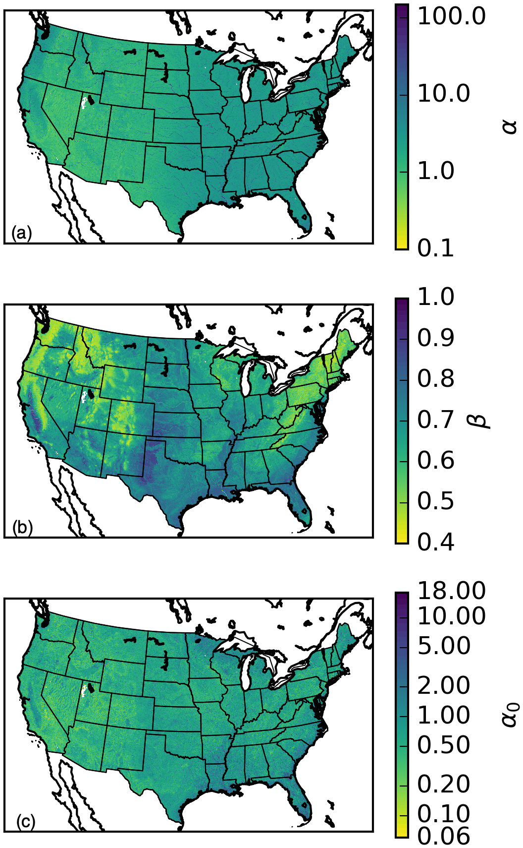
Figure 5 Spatial distributions of the kinematic wave parameters (a) α, (b) β, and (c) α₀ used over the CONUS in this study.

EF5 was run for the period from 2001 through 2011 for USGS stream gauges with a basin area under 1000 km². There are 4366 stream gauges over the CONUS that meet this basin area threshold. The MRMS reanalysis precipitation rates with a time step of 5 min were used as the precipitation forcing for EF5. The PET data were climatological monthly mean data derived from Koren et al. (1998). EF5 was run with a 5 min time step producing 5 min output-simulated time series. The resulting simulations took 1 week of computer time for the EF5/CREST combination and 2.5 weeks of computer time for EF5/SAC-SMA, illustrating the relative differences in complexity and performance between the two water balance models. The year 2001 was used as a model warmup period, and so results will only be presented from 2002 through 2011.

3.2 CONUS bulk simulation validation

A bulk analysis was performed to evaluate the skill of the modeling system at every USGS gauge with a basin area less than 1000 km². The time series from the EF5 simulations can be evaluated as a function of the performance at each individual stream gauge. This information can then be viewed in bulk to gather a sense of how the system performs spatially in terms of the overall mass of water, and the correlation between simulated and observed events. The accuracy of the simulations is judged using Pearson's linear correlation coefficient (CC), defined as

$$\begin{array}{}\text{(26)}& \text{CC}={\displaystyle \frac{\text{Cov}({\mathit{Q}}_{\mathrm{sim}},{\mathit{Q}}_{\mathrm{obs}})}{\sqrt{\text{Var}\left({\mathit{Q}}_{\mathrm{sim}}\right)\text{Var}\left({\mathit{Q}}_{\mathrm{obs}}\right)}}},\end{array}$$

where Q_sim is the simulated discharge value and Q_obs is the USGS-measured discharge value. The values for correlation coefficient can range from −1 to 1, with 1 being the best. The normalized bias of the simulations is computed using

$$\begin{array}{}\text{(27)}& \text{bias}={\displaystyle \frac{{\sum }_{i=\mathrm{1}}^N({\mathit{Q}}_{\mathrm{sim}}^i-{\mathit{Q}}_{\mathrm{obs}}^i)}{{\sum }_{i=\mathrm{1}}^N{\mathit{Q}}_{\mathrm{obs}}^i}}\cdot \mathrm{100},\end{array}$$

where N is the number of observations in the discharge time series. Normalized bias ranges from −100 % to ∞, with 0 % being the best. Finally the Nash–Sutcliffe coefficient of efficiency (NSE; Nash and Sutcliffe, 1970), commonly used as a skill metric to define simulations that have better skill than the mean of the observations would have, is computed as

$$\begin{array}{}\text{(28)}& \text{nse}=\mathrm{1}-{\displaystyle \frac{{\sum }_{i=\mathrm{1}}^N({\mathit{Q}}_{\mathrm{sim}}^i-{\mathit{Q}}_{\mathrm{obs}}^i{)}^{\mathrm{2}}}{{\sum }_{i=\mathrm{1}}^N({\mathit{Q}}_{\mathrm{obs}}^i-\stackrel{\mathrm{‾}}{{\mathit{Q}}_{\mathrm{obs}}}{)}^{\mathrm{2}}}},\end{array}$$

where $\stackrel{\mathrm{‾}}{{\mathit{Q}}_{\mathrm{obs}}}$ is the mean of the discharge observations for this station. The values for NSE range from −∞ to 1 with 1 being a simulation perfectly matching the observations.

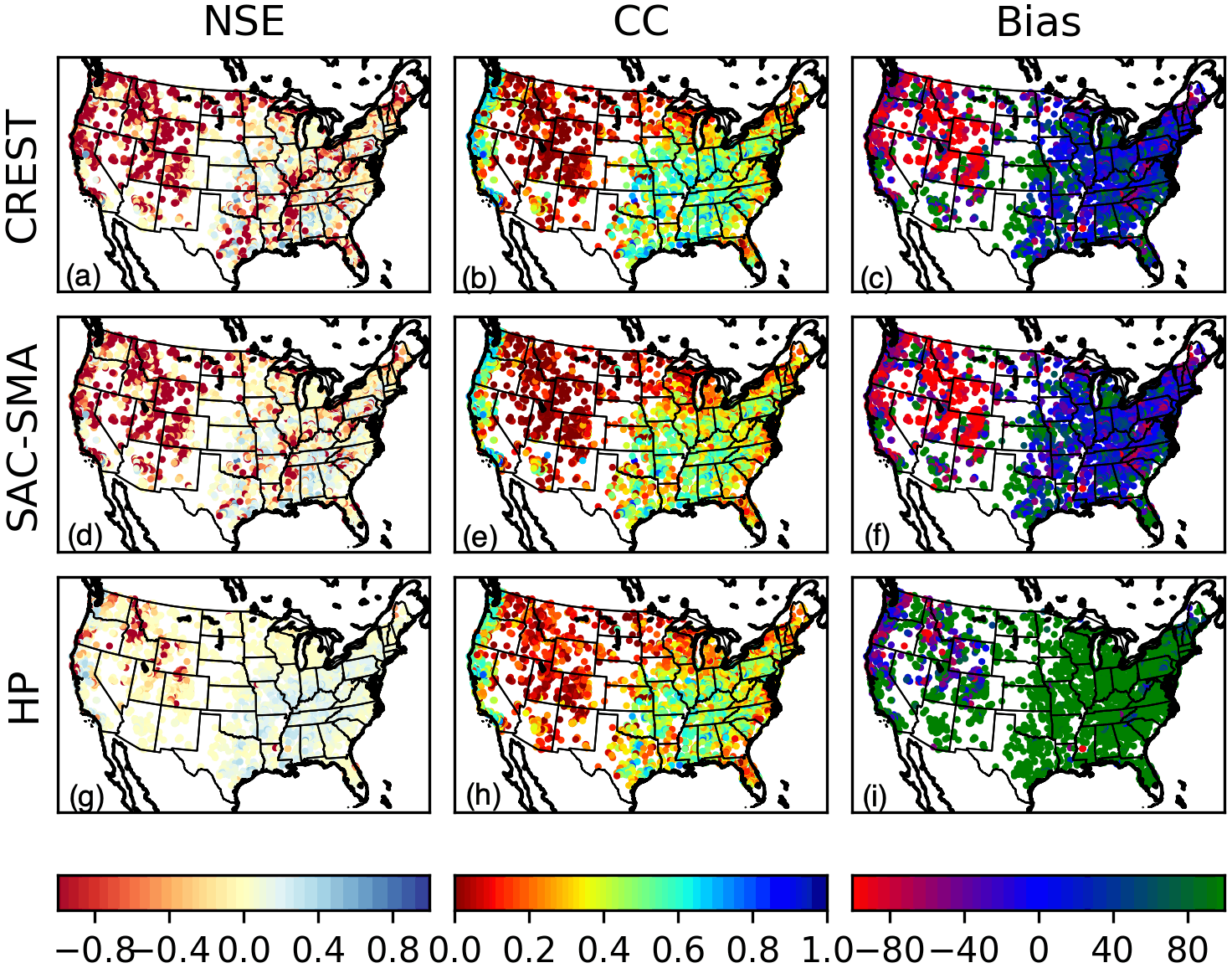
Figure 6 The spatial distribution of NSE, CC, and normalized bias computed against USGS observations for all gauges with drainage areas less than 1000 km² for (a)–(c) CREST, (d)–(f) SAC-SMA, and (g)–(i) HP models.

Table 6 Statistical summary of EF5 performance.

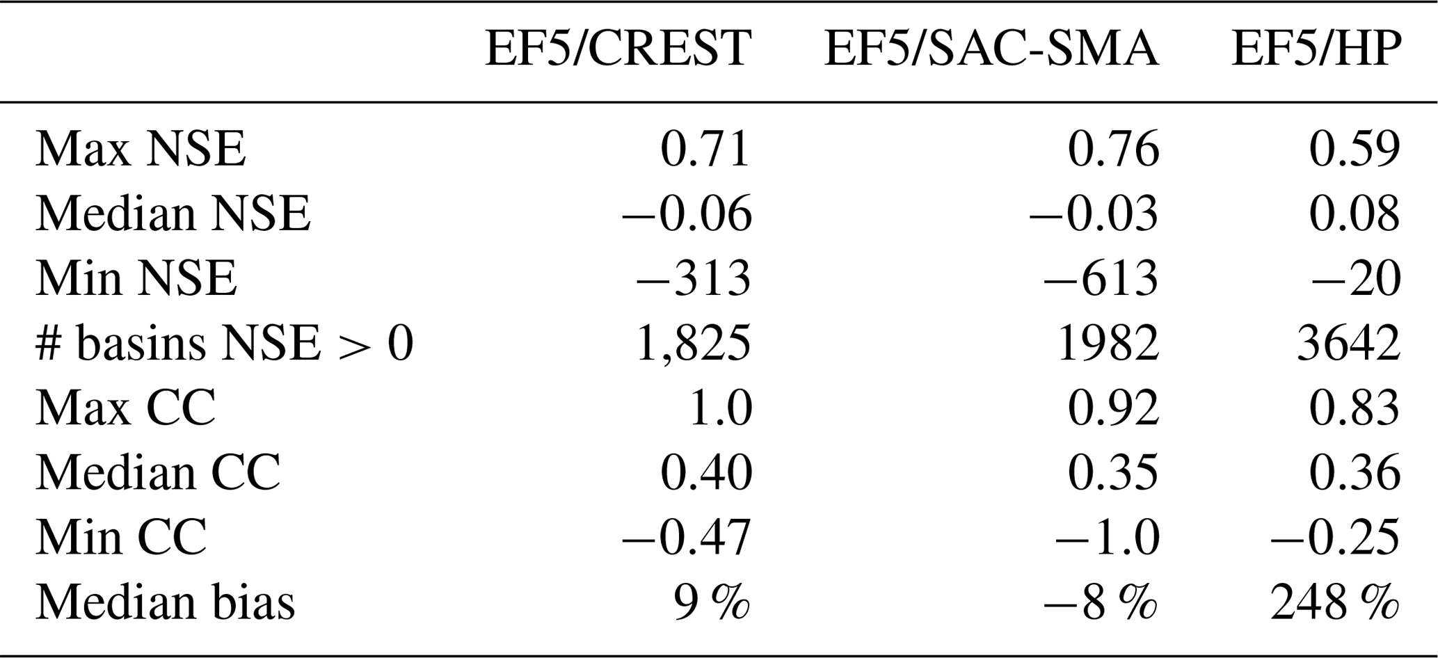
Figure 6 shows the spatial distribution of NSE, CC, and normalized bias for the three simulations. The maximum, median, and minimum values for NSE, CC, and bias are summarized in Table 6. Overall, the water balance modules yield comparable performance with a few notable patterns. There is a notable drop in accuracy and negative bias in the intermountain West region according to all three models. The relatively poor performance here is due to inaccurate precipitation forcings. First, radar-based precipitation estimates face challenges due to intervening blockages by the mountains and greater distances between radars (Maddox et al., 2002). Second, there is a large portion of precipitation that falls as snow in this high-elevation region. While the parent MRMS precipitation forcings separate frozen and liquid precipitation, EF5 did not consider snow processes in this study. As such, results in these regions should be used with caution when frozen-precipitation processes are active.

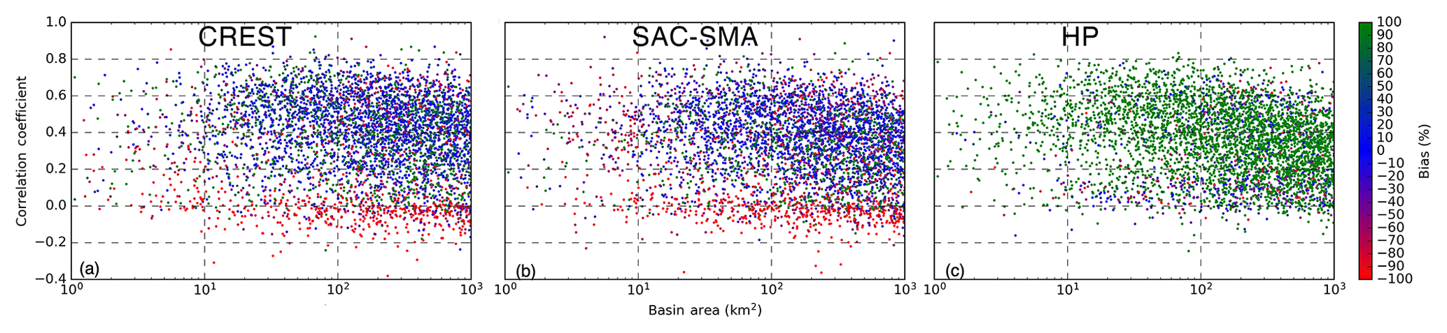
Figure 7 The correlation coefficient and normalized bias versus contributing drainage area for all gauges with drainage areas less than 1000 km² for (a) CREST, (b) SAC-SMA, and (c) HP models.

The results from this study using EF5/CREST, EF5/SAC-SMA, and EF5/HP – all with a priori, uncalibrated parameters and coupled to the kinematic wave routing scheme – show no significant systematic errors as a function of watershed scale. It took 1 week of computer time to simulate streamflow across the CONUS with rainfall estimates being input to the models at a 5 min frequency. The overall skill of the system is reasonable given the lack of optimized parameters, and on some watersheds the skill is equivalent to that expected with a calibrated hydrologic model. The results in Fig. 7 show no significant trend in accuracy as a function of basin area for the range of flash flood basins from 1 to 1000 km². The EF5/HP model yields a worst-case scenario and exhibits large positive bias for most watersheds, which is expected behavior for a completely impervious land surface. The EF5/HP model provides an upper envelope when used as a member of an ensemble, which is useful for diagnosing errors in precipitation input forcing, approximating the behavior of runoff on burn areas, and diagnosing situations in which the soils are completely saturated.

4 Summary and future work

To further the goal of producing accurate, precise, and timely flash flood warnings while utilizing new precipitation datasets, a new high-resolution distributed hydrologic modeling platform, EF5, was created to facilitate this process. EF5 features flexible options for choosing which water balance models and routing schemes to simulate with or whether to run all of them to generate a hydrologic ensemble. The resulting software package was used for generating 5 min simulations for 4366 gauge locations across the CONUS with uncalibrated, a priori parameters for the EF5/CREST, EF5/SAC-SMA, and EF5/HP water balance models coupled to kinematic wave routing. Furthermore, EF5 is being used for training, capacity building, and operational forecasting (Clark et al., 2017). EF5/CREST and EF5/SAC-SMA run with uncalibrated, a priori parameters over the CONUS, and MRMS precipitation forcing produces skillful simulations except in mountainous regions, with NSE scores up to 0.76. EF5/HP produces useful estimates for worst-case scenarios if all rainfall is converted into runoff such as over burn areas, in heavily urbanized watersheds, or in situations in which the soils are saturated.

The future for EF5, hydrologic modeling, and developing climatologies of flash floods is extremely promising. EF5 is being used to power the distributed hydrologic models in the FLASH system (Gourley et al., 2017), where NWS forecasters are using it in a warning decision support role. The operational version of EF5 runs across the conterminous United States and territories at 1 km spatial resolution and frequency of every 10 min. Future developments for EF5 may include diffusive wave routing to better handle shallow slope basins and a parameterization for reservoirs so that they can also be accommodated. EF5 currently has a snow module, but a priori parameter development is required before it can be deployed across the CONUS and globally. Continued improvements to EF5 are a must to ensure it remains accessible to all users in the future. A better graphical user interface on the Windows operating system may improve classroom and workshop usability. Solutions for containerizing EF5 such as Docker should be explored to see if there are significant advantages to this workflow.

In the future, new observational platforms will be necessary to collect the observations needed to validate distributed hydrologic models. As the spatiotemporal resolution of hydrologic models increases, the need for validating observations also increases. These new observations could come from augmentations of existing datasets such as with stream radars that can map the channel cross section, surface water velocity, and stage. Unpiloted aerial systems have a promising role in the future as well; an automated platform that maps out flood waters in real time would be invaluable as a dataset for verifying hydrologic models.