One-dimensional models of radiation transfer in heterogeneous canopies: a review, re-evaluation, and improved model

Despite recent advances in the development of detailed plant radiative transfer models, large-scale canopy models generally still rely on simplified one-dimensional (1-D) radiation models based on assumptions of horizontal homogeneity, including dynamic ecosystem models, crop models, and global circulation models. In an attempt to incorporate the effects of vegetation heterogeneity or “clumping” within these simple models, an empirical clumping factor, commonly denoted by the symbol Ω, is often used to effectively reduce the overall leaf area density and/or index value that is fed into the model. While the simplicity of this approach makes it attractive, Ω cannot in general be readily estimated for a particular canopy architecture and instead requires radiation interception data in order to invert for Ω. Numerous simplified geometric models have been previously proposed, but their inherent assumptions are difficult to evaluate due to the challenge of validating heterogeneous canopy models based on field data because of the high uncertainty in radiative flux measurements and geometric inputs. This work provides a critical review of the origin and theory of models for radiation interception in heterogeneous canopies and an objective comparison of their performance. Rather than evaluating their performance using field data, where uncertainty in the measured model inputs and outputs can be comparable to the uncertainty in the model itself, the models were evaluated by comparing against simulated data generated by a three-dimensional leaf-resolving model in which the exact inputs are known. A new model is proposed that generalizes existing theory and is shown to perform very well across a wide range of canopy types and ground cover fractions.

1 Introduction

Solar radiation drives plant growth and function, and thus quantification of fluxes of absorbed radiation is a critical component of describing a wide range of plant biophysical processes. Solar radiation provides the energy for plants to carry out photosynthesis and drives the energy balance and, thus, the temperature of plant organs (Jones, 2014). As a result, nearly any attempt to quantify plant development in the natural environment involves acquiring information regarding radiation interception. The unobstructed incoming solar radiation flux is relatively easy to measure; however, because of the dense and complex orientation of vegetative elements, characterizing leaf-level radiative fluxes is much more challenging (Pearcy, 1989).

Rather than representing the absorption of radiation by individual leaves, radiation transport is most commonly described statistically at the canopy level through the use of models. Using an analogy to absorption of radiation due to a continuous particle-filled medium, classical radiation transfer theory can be readily adapted to quantify radiation transport within a continuous medium of vegetation as pioneered by Monsi and Saeki (1953). Assuming that scattering of radiation is negligible and that leaf positions follow a uniform random distribution in space, the governing equation for radiation attenuation within a medium of vegetation is given by Beer's law (also called Beer–Lambert law or Beer–Lambert–Bouguer law), which predicts an exponential decline in radiation with propagation distance. The importance of this equation in plant ecosystem models cannot be overstated and is incorporated within nearly every land surface model (e.g., Sellers et al., 1996; Kowalczyk et al., 2006; Clark et al., 2011; Lawrence et al., 2019), crop model (e.g., Jones et al., 2003; Keating et al., 2003; Stöckle et al., 2003; Soltani and Sinclair, 2012), and dynamic vegetation/ecosystem model (e.g., Bonan et al., 2003; Krinner et al., 2005).

Perhaps one of the biggest challenges in the application of Beer's law is that it inherently assumes that vegetation is homogeneous in space, but many, if not most, of the plant systems in which it is applied are not homogeneous. For example, crops, savannas, coniferous forests, and even tropical forests can have significant heterogeneity due to gaps that freely allow for radiation penetration with near-zero probability of interception (Campbell and Norman, 1998; Bohrer et al., 2009). Crop canopies are inherently sparse early in their development and can remain so in many perennial cropping systems such as orchards and vineyards. A recent study by Ponce de León and Bailey (2019) quantified errors in the prediction of absorbed radiation using Beer's law for a variety of canopy architectures and found that errors could reach 100 % in canopies where the between-plant spacing was larger than the canopy height.

An incredibly wide range of approaches of varying complexity have been used to develop radiation transfer models applicable to heterogeneous canopies. The most robust and computationally expensive approach is to explicitly resolve the most important scales of heterogeneity, such as with a leaf-resolving model (e.g., Pearcy and Yang, 1996; Chelle and Andrieu, 1998; Bailey, 2018; Henke and Buck-Sorlin, 2018) or a 3-D model that resolves crown-scale (e.g., Wang and Jarvis, 1990; Cescatti, 1997; Stadt and Lieffers, 2000) or sub-crown-scale heterogeneity (e.g., Kimes and Kirchner, 1982; Sinoquet et al., 2001; Gastellu-Etchegorry et al., 2004; Bailey et al., 2014). To further reduce model complexity, a class of geometric models has been developed that explicitly or statistically represents heterogeneity at the scale of plant crowns in order to predict whole-canopy radiation absorption (e.g., Norman and Welles, 1983; Li and Strahler, 1988; Nilson, 1999; Yang et al., 2001; Ni-Meister et al., 2010). A yet more simplified and perhaps the most commonly used approach is to include an empirical clumping factor Ω in the exponential argument of Beer's law that effectively scales the radiation attenuation coefficient based on the level of vegetation clumping (Nilson, 1971; Chen and Black, 1991; Black et al., 1991). Clumping usually results in an overestimation of radiation absorption when a model based on Beer's law is used (Ponce de León and Bailey, 2019), and thus setting Ω<1 reduces the effective attenuation coefficient within Beer's law, which corrects for this overestimation.

Despite the wealth of available models for quantifying radiative transfer in heterogeneous canopies, a critical knowledge gap still exists in which it is usually unclear which model is suited for a particular application, and even a general sense of the errors associated with certain model assumptions is often unknown. Models are commonly selected for historical reasons, based on ease of implementation, availability of computational resources versus domain size, or presence of perceived errors given the particular model assumptions. This uncertainty is driven by the fact that obtaining robust validation data is exceptionally difficult, and often uncertainty in model inputs is comparable to uncertainty in the model itself. Offsetting errors and coefficient “tuning” can lead to models that perform exceptionally well in a particular case but may produce unacceptably large errors when applied generally. These difficulties have led to a number of model intercomparison exercises in which simulations are performed of synthetic or artificial canopy cases (Pinty et al., 2001, 2004; Widlowski et al., 2007, 2013). This eliminates ambiguity in model inputs in order to enable a more objective comparison; however, the “exact” solution is still unknown.

This paper presents a critical re-evaluation of the theoretical basis of simplified one-dimensional (1-D) models of radiation transfer in heterogeneous canopies based on Beer's law. Due to the difficulties in objectively comparing and evaluating models based on field data, the performance of various models was explored by applying them in virtually generated canopies where the inputs are exactly known and comparing against the output of a detailed leaf-resolving model. The goal of the study was to better understand the implications of radiation model assumptions and uncertainty in model inputs in a wide range of canopy geometries in order to guide model selection in future applications.

2 Theory

2.1 Modeling radiative transfer in plant canopies

The governing equation for radiation transfer in a participating medium is the radiative transfer equation (RTE; Modest, 2013), which describes the rate of change of radiative intensity along a given direction s^′

$$\begin{array}{ll}{\displaystyle \frac{\mathrm{d}I(\mathit{r};{\mathit{s}}^{\prime })}{\mathrm{d}\mathit{r}}}=& {\displaystyle }-\mathit{\kappa }I(\mathit{r};{\mathit{s}}^{\prime })-{\mathit{\sigma }}_{s}I(\mathit{r};{\mathit{s}}^{\prime })+\mathit{\kappa }{I}_b\left(\mathit{r}\right)\\ \text{(1)}& {\displaystyle }& {\displaystyle }+{\mathit{\sigma }}_s\underset{\mathrm{4}\mathit{\pi }}{\int }I(\mathit{r};\mathit{s})\left[{\displaystyle \frac{\mathrm{\Phi }(\mathit{r};{\mathit{s}}^{\prime },\mathit{s})}{\mathrm{4}\mathit{\pi }}}\right]\mathrm{d}\mathrm{\Omega },\end{array}$$

where $I(\mathit{r};{\mathit{s}}^{\prime })$ is the radiative intensity at position r along the direction of propagation s^′; κ and σ_s are the radiation absorption and scattering coefficients of the medium, respectively, I_b(r) is the blackbody intensity of emission at position r, $\mathrm{\Phi }(\mathit{r};{\mathit{s}}^{\prime },\mathit{s})$ is the scattering phase function at position r for propagation direction s^′ and scattered direction s, and dΩ is a differential solid angle.

If scattering and emission within the medium are neglected (i.e., ${\mathit{\sigma }}_s=I_b=\mathrm{0}$), the RTE can be written more simply as

$$\begin{array}{}\text{(2)}& {\displaystyle \frac{\partial I(\mathit{r};{\mathit{s}}^{\prime })}{\partial \mathit{r}}}=-\mathit{\kappa }I(\mathit{r};{\mathit{s}}^{\prime }).\end{array}$$

This equation can be integrated along s^′ from a distance of r=0 to r to yield

$$\begin{array}{}\text{(3)}& I(r;{\mathit{s}}^{\prime })=I(\mathrm{0};{\mathit{s}}^{\prime })\exp \left(-\mathit{\kappa }r\right).\end{array}$$

The attenuation coefficient can be interpreted physically as the cross-sectional area of radiation-absorbing objects projected in the direction s^′ per unit volume of the medium. For a medium of leaves, the attenuation coefficient is given by

$$\begin{array}{}\text{(4)}& \mathit{\kappa }=G\left({\mathit{s}}^{\prime }\right)a,\end{array}$$

where a is the one-sided leaf area density (m² leaf area per m³ canopy), and G(s^′) is the fraction of total leaf area projected in the direction of s^′. It is frequently assumed that the attenuation coefficient does not have azimuthal dependence, and therefore the G function can be written as G(θ), where θ is the zenithal angle of the direction of radiation propagation. The probability P of a beam of radiation, inclined at an angle of θ, intersecting a leaf within a homogeneous volume of vegetation after propagating a distance of r can thus be written as

$$\begin{array}{}\text{(5)}& P\left(r\right)=\left[\mathrm{1}-\exp \left(-G\left(\mathit{\theta }\right)ar\right)\right].\end{array}$$

For a canopy that extends indefinitely in the horizontal direction, the propagation distance r can be rewritten in terms of the canopy height h as $r=h/\cos \mathit{\theta }$. Substituting this relation for r and noting that the leaf area index (LAI) is defined as a h=L (if a is constant) yields the common form of Beer's law applied to plant canopy systems

$$\begin{array}{}\text{(6)}& P=\left[\mathrm{1}-\exp \left(-{\displaystyle \frac{G\left(\mathit{\theta }\right)L}{\cos \mathit{\theta }}}\right)\right].\end{array}$$

2.2 Application of Beer's law in heterogeneous canopies

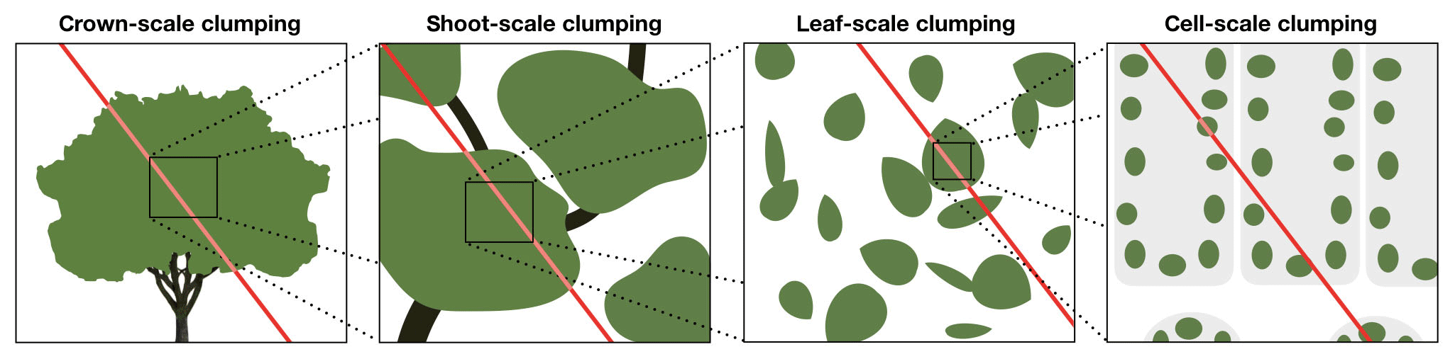
As introduced previously, Eq. (6) is only valid within a homogeneous volume of vegetation – i.e., leaves are uniformly distributed in space. In reality, essentially all canopies have heterogeneity or clumping at a number of scales. There is inherent clumping at the leaf scale, as leaves are discrete surfaces unlike arbitrarily small gas molecules, and thus even at this scale, the assumptions of Beer's law are violated. Above the leaf scale, leaves are grouped around shoots or spurs, creating heterogeneity at a larger scale. Shoots are grouped around main branches or the plant stem, creating yet another scale of heterogeneity. Large-scale clumping typically exists due to gaps between individual trees or due to clearings in the canopy.

In a strict sense, each of these scales of heterogeneity violates the assumptions of Beer's law. One obvious means of dealing with this heterogeneity is to use a more complicated model that explicitly resolves the important scales of heterogeneity, such as a “multilayer” model that resolves heterogeneity in the vertical direction (e.g., Meyers and Paw U, 1987; Leuning et al., 1995), a 3-D model that resolves plant-scale heterogeneity (e.g., Wang and Jarvis, 1990; Cescatti, 1997; Stadt and Lieffers, 2000), a 3-D voxel-based model that resolves sub-plant heterogeneity (e.g., Kimes and Kirchner, 1982; Sinoquet et al., 2001; Gastellu-Etchegorry et al., 2004; Bailey et al., 2014), or a 3-D leaf-level model that resolves heterogeneity at the leaf scale (e.g., Pearcy and Yang, 1996; Chelle and Andrieu, 1998; Bailey, 2018; Henke and Buck-Sorlin, 2018). However, each of these models incurs a level of computational expense that may be unacceptable for global-scale models or crop models, which require the high efficiency that is provided by simpler models based on Beer's law. As a compromise, numerous geometric models have been proposed that calculate radiation interception using analytical geometric solutions along with simplifying assumptions of the basic shape of canopy elements, such as a hedgerow crop (Tsubo and Walker, 2002; Annandale et al., 2004), spherical and/or ellipsoidal crowns (Norman and Welles, 1983; Li and Strahler, 1988; Ni-Meister et al., 2010), or conical crowns (Kuuluvainen and Pukkala, 1987; Van Gerwen et al., 1987; Li and Strahler, 1988). However, these models do not necessarily generalize to an arbitrary canopy, and in many cases the choice of the average geometric input parameters may be unclear, and thus their determination may require an empirical inversion (e.g., Li and Strahler, 1988).

2.3 Ω canopy clumping factor approach for incorporating vegetative heterogeneity

The issue of incorporating the effects of clumping in Beer's law models gained a heightened level of attention in the early 1990s from investigators looking to use radiation measurements to invert Beer's law for leaf area index (LAI) values (Black et al., 1991; Chen and Black, 1991, 1993). Canopy nonrandomness or clumping causes underestimation of LAI values inferred in this way, and thus there was a pressing need for a theoretical formulation that could remove the effects of clumping within the inversion procedure, which was also mathematically simple enough that it could be easily inverted for LAI. In an early attempt at applying such a correction, Chen and Black (1991) introduced an empirical coefficient within Beer's law which was termed the “clumping index” and denoted by Ω.

$$\begin{array}{}\text{(7)}& P=\left[\mathrm{1}-\exp \left(-{\displaystyle \frac{G\left(\mathit{\theta }\right)\mathrm{\Omega }L}{\cos \mathit{\theta }}}\right)\right]\end{array}$$

Chen and Black (1991) references the early work of Nilson (1971) that originally derived this relationship (its Eq. 25, with the clumping parameter denoted by λ). Nilson (1971) derived this relationship for “stands with a clumped dispersion of foliage” using a Markov chain model. The assumption was that the probability of interception at any point also depends to some degree on the probability of interception at a previous location, with the level of dependence described by Ω (or λ using the notation of Nilson, 1971). This approach, however, does not explicitly allow for large-scale gaps in vegetation such as crown-scale clumping, but rather it assumes that there is some quasi-homogeneous medium with regular and repeating variation in vegetation density.

Within a few years, the clumping factor approach was incorporated into radiation transport models (e.g., Chen et al., 1999; Kucharik et al., 1999; Kull and Tulva, 2000) and quickly became ubiquitous in its application within land surface models (Krayenhoff et al., 2014; Han et al., 2015), remote sensing inversion models (e.g., Kuusk and Nilson, 2000; Anderson et al., 2005; Tao et al., 2016), crop models (e.g., Rizzalli et al., 2002; Teh, 2006; Jin et al., 2016), and ecological models (e.g., Walcroft et al., 2005; Ni-Meister et al., 2010). These applications generally necessitate simple and highly efficient models for radiation interception, and thus Eq. (7) provides a reasonable compromise between model complexity and accuracy. An additional benefit is that it has only one empirical parameter (Ω) to be specified that can incorporate the effects of vegetation heterogeneity.

Despite the seemingly attractive simplicity of the clumping factor approach, it has many limitations. Foremost of these limitations is that in general the clumping factor Ω has a strong dependence on every other variable in Eq. (7), namely θ, L, and G (Chen et al., 2008; Ni-Meister et al., 2010). In effect, specifying Ω requires knowledge of P. Thus, if P is already known, there is no need to determine Ω and apply Eq. (7) in the first place. Empirical modeling of Ω (e.g., Campbell and Norman, 1998; Kucharik et al., 1997, 1999) is effectively a matter of empirically modeling P. If the leaf orientation and heterogeneity are both isotropic, then G and Ω would no longer have θ dependence. In this case, the product G Ω L becomes inseparable, and the canopy begins to appear homogeneous with attenuation determined by the value of G Ω L. The probability of interception can then be written as

$$\begin{array}{}\text{(8)}& P=\left[\mathrm{1}-\exp \left(-{\displaystyle \frac{{\mathrm{\Omega }}^{\prime }}{\cos \mathit{\theta }}}\right)\right],\end{array}$$

where ${\mathrm{\Omega }}^{\prime }=G\mathrm{\Omega }L=\text{const}$. Thus, if P is known for any particular θ, Ω^′ can be determined.

2.4 Geometric modeling of radiative transfer in heterogeneous vegetation

Figure 1 Hierarchical scales of spatial aggregation or clumping in a plant canopy.

2.4.1 Direct (collimated) radiation component

Beer's law is only explicitly valid in a medium in which the probability of radiation interception is homogeneous over some discrete scale. Thus, in order to apply Beer's law in heterogeneous vegetation, we must segment the canopy into sections over which we can assume that the vegetative elements are homogeneous in space. In a typical canopy, there may be multiple scales over which this is applicable (Fig. 1). At the leaf scale, the probability of interception is approximately homogeneous and is equal to the leaf absorptivity. For a clump of leaves (e.g., a shoot), the probability of interception may be assumed approximately homogeneous and is given by Beer's law (Eq. 6). There may be large gaps between individual shoots, which invalidate Eq. (6), but the overall distribution of shoots across a crown may be approximately homogeneous, and thus the probability that a photon intersects an individual shoot may follow Beer's law but with an augmented attenuation coefficient. Finally, there may be large gaps between crowns that invalidate Eq. (6), but this heterogeneity may be regular and repeating, and thus the probability that a photon intersects an individual crown may be described by Beer's law.

The cumulative probability of photon interception can be viewed as an aggregation of many “clumps” consisting of a homogeneous medium of elements at a smaller scale. For each clump, the probability of a photon intersection is assumed homogeneous in space, and thus the probability of interception can be assumed constant. In this case, the cumulative probability of interception over all clumping levels is

$$\begin{array}{}\text{(9)}& P=\prod _{i=\mathrm{1}}^{N_{\text{c}}}{P}_i,\end{array}$$

where P is the cumulative probability of interception over all scales, N_c is the total number of clumping levels, and P_i is the probability of intersecting the ith clumping level.

The product of Eq. (9) could be applied in any number of ways depending on the scale at which various probabilities of interception are known. In the example given below, we will follow an approach similar to Nilson (1999) in which the probability of interception within a single plant crown is determined, then repeated N_c times for each crown in the canopy that the beam of radiation traverses. Accordingly, the canopy is segmented into crown “envelopes” (cf. Nilson, 1992), each of which is conceptualized to a volume encompassing all vegetation within the plant, inside which it is assumed that vegetation is homogeneous.

The probability of a beam of radiation intersecting a single crown is the product of the probability of intersecting the crown envelope and the probability of intersecting a leaf within the envelope. At a solar zenith angle of zero, the probability of intersecting the crown envelope is given by the ground cover fraction f_c, which is the area of the crown envelope shadow at a solar zenith of zero S(0) divided by the average plan area of ground associated with a single plant. For spherical or cylindrical crowns of radius R and spacing s, the ground cover fraction is $f_{\text{c}}=S\left(\mathrm{0}\right)/s^{\mathrm{2}}=\mathit{\pi }{R}^{\mathrm{2}}/s^{\mathrm{2}}$. The probability that a beam intersects a leaf within a single crown is simply given by Eq. (5), with r being the path length through the crown. Because of the nonlinearity of this equation, we cannot simply compute the average r over the crown and substitute it into Eq. (5). Rather, Eq. (5) should be weighted by the probability that a beam path length through the crown is equal to some value r. Thus, the probability P_ℓ that a ray passing through a crown envelope intersects a leaf can be written as

$$\begin{array}{}\text{(10)}& P_{\mathrm{\ell }}=\int p(r;\mathit{\theta })\left[\mathrm{1}-\exp \left(-G\left(\mathit{\theta }\right)ar\right)\right]\mathrm{d}r,\end{array}$$

where p(r;θ) is the probability that the beam path length through a crown is equal to r for a solar zenith angle of θ. Li and Strahler (1988) showed that for a sphere of radius R, $p\left(r\right)=r/\mathrm{2}{R}^{\mathrm{2}}$ (no θ dependence for spheres), with $\mathrm{0}\le r\le \mathrm{2}R$, and thus the limits on the integral in Eq. (10) become 0 to 2R. For other shapes, analytical expressions for p(r;θ) become tedious or impossible to derive. However, the integral expressions given by Li and Strahler (1988) for p(r;θ) can be evaluated numerically. The approach used here was to perform line–cylinder intersection tests (which are analytical; Suffern, 2007) for a large number of lines inclined in the direction of the sun, which allows for population of a probability distribution. A similar approach could be used for ellipsoids (equations given in Norman and Welles, 1983).

In order to use the above expression to calculate the probability of interception for an entire canopy of repeated crowns, we must assume a statistical distribution that describes the probability of intersecting a crown envelope within a canopy. The two distributions that are commonly chosen are the binomial distribution (Nilson, 1971, 1999) or Poisson distribution (Nilson, 1971, 1999; Li and Strahler, 1988). If a (positive) binomial distribution is assumed, the interception probability for the entire canopy is

$$\begin{array}{}\text{(11)}& P=\mathrm{1}-{\left(\mathrm{1}-f_{\text{c}}{P}_{\mathrm{\ell }}\right)}^{N_{\text{c}}},\end{array}$$

where N_c is the number of crowns intersected by the radiation beam. Effectively this amounts to saying that the probability of not intercepting an individual crown is 1−f_cP_ℓ, which is compounded N_c times. When the solar zenith is zero, this means that N_c=1, and thus Eq. (11) correctly yields a probability of intersection of f_cP_ℓ.

If a Poisson distribution is assumed, the interception probability for the entire canopy is

$$\begin{array}{}\text{(12)}& P=\mathrm{1}-\exp \left(-f_{\text{c}}{P}_{\mathrm{\ell }}{N}_{\text{c}}\right).\end{array}$$

Application of this model effectively assumes that crowns act like a homogeneous medium of objects that repeats in all directions, analogous to individual molecules in a gas. When the sun direction is near zenith, this assumption is poor as the canopy consists of only a single layer of objects. In this case, the probability of intersection should be f_cP_ℓ, but Eq. (12) incorrectly gives a value of $\mathrm{1}-\exp \left(-f_{\text{c}}{P}_{\mathrm{\ell }}\right)$, which is always less than f_cP_ℓ.

Nilson (1999) estimated N_c as the ratio of the projected crown shadow area S(θ) to the projected crown shadow area at a solar zenith of zero S(0) (he used the symbol K rather than N). For spherical crowns, $S\left(\mathit{\theta }\right)=S\left(\mathrm{0}\right)/\cos \mathit{\theta }=\mathit{\pi }{R}^{\mathrm{2}}/\cos \mathit{\theta }$. For ellipsoidal crowns with horizontal radius of R and height H, $S\left(\mathit{\theta }\right)=\mathit{\pi }{R}^{\mathrm{2}}\sqrt{\mathrm{1}+(H/\mathrm{2}R{)}^{\mathrm{2}}{\tan }^{\mathrm{2}}\mathit{\theta }}$ (Nilson, 1999). For cylindrical crowns of radius R and height H, S(θ) is well approximated by $S\left(\mathit{\theta }\right)=\mathit{\pi }{R}^{\mathrm{2}}+\mathrm{2}RH\tan \mathit{\theta }$.

This approach for estimating N_c works well if the crowns are randomly or uniformly distributed in space, and thus N_c is azimuthally symmetric. If crowns are oriented in rows, the relationship for N_c changes with azimuth. To account for this, we propose the following. Consider the case in which crowns are spaced at a distance of s_p (plant spacing) in the direction of radiation propagation and spaced at a distance of s_r (row spacing) in the direction normal to the direction of propagation. The azimuthally symmetric model of $N_{\text{c}}=S\left(\mathit{\theta }\right)/S\left(\mathrm{0}\right)$ can be applied, provided that the asymmetry in the actual ground cover fraction is properly accounted for. This is accomplished by (1) calculating the ground cover fraction using the crown spacing in the direction of radiation propagation, which in this example is $f_{\text{c}}=S\left(\mathrm{0}\right)/s_{\text{p}}^{\mathrm{2}}$, and (2) multiplying the final interception probability by the ratio of the isotropic crown footprint area ($s_{\text{p}}^{\mathrm{2}}$ in this example) to the actual crown footprint area (s_ps_r in this example).

To generalize this approach, we take the azimuthally symmetric plant spacing s to be $s=s_{\text{r}}{\sin }^{\mathrm{2}}\mathit{\phi }+s_{\text{p}}{\cos }^{\mathrm{2}}\mathit{\phi }$, where φ is the azimuthal angle between the sun direction and the row direction. Equation (11) can then be generalized to

$$\begin{array}{}\text{(13)}& P={\displaystyle \frac{s^{\mathrm{2}}}{s_{\text{r}}{s}_{\text{p}}}}\left[\mathrm{1}-{\left(\mathrm{1}-{\displaystyle \frac{S\left(\mathrm{0}\right)}{s^{\mathrm{2}}}}{P}_{\mathrm{\ell }}\right)}^{N_{\text{c}}}\right].\end{array}$$

It is noted that when s_r=s_p, Eq. (13) reduces back to Eq. (11). Table 1 provides a summary of inputs and equations needed to implement Eq. (13) for different geometries.

Table 1 Summary of inputs and equations needed to implement the BINOM model for canopies with spherical or cylindrical crowns.

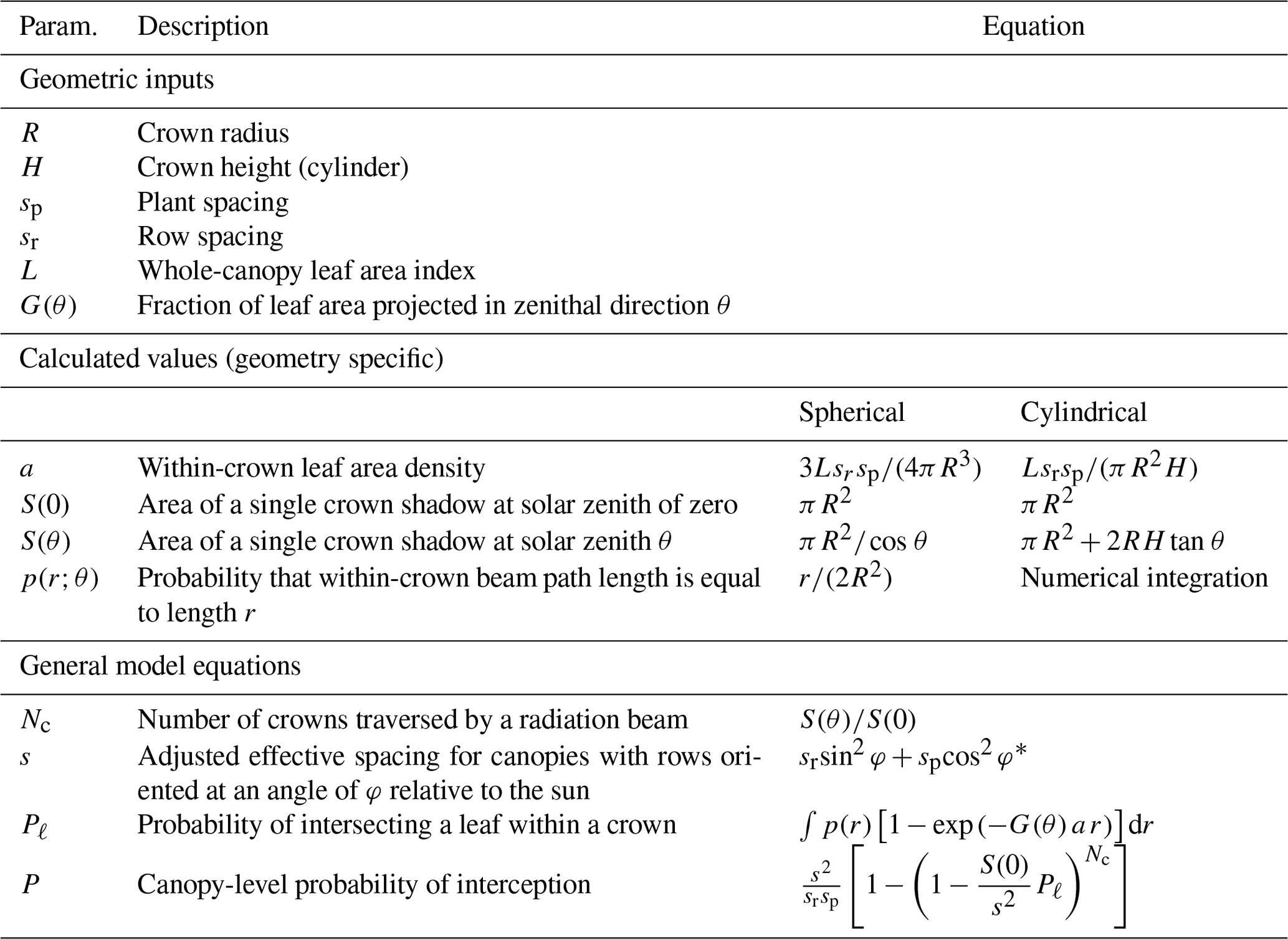
^* If plant spacing is azimuthally symmetric (e.g., random), $s=s_{\text{r}}=s_{\text{p}}$.

(see Nilson, 1999)(see Nilson, 1999)(see Ni-Meister et al., 2010)(see Campbell and Norman, 1998)

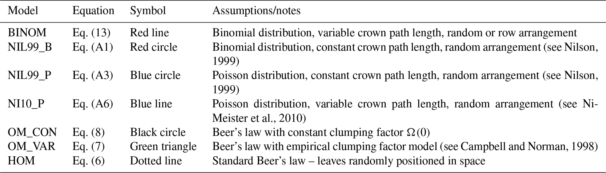
Table 2 Summary of 1-D models of radiation interception considered in this study.

2.4.2 Diffuse radiation component

As introduced above, the RTE (Eq. 1) and thus Beer's law (Eq. 6) are only explicitly valid along a single direction of radiation propagation, and therefore these equations as written can only be applied for collimated radiation (e.g., direct solar radiation). It is common to adapt Beer's law for diffuse radiation conditions by substituting a modified diffuse radiation attenuation coefficient that is usually assumed to be constant for a particular canopy (e.g., DePury and Farquhar, 1997; Wang and Leuning, 1998; Drewry et al., 2010). However, for the reasons above, this approach is not consistent with the assumptions of Beer's law.

A more robust approach for representing incoming diffuse radiation from the sky is to apply Beer's law to any given direction in the sky and integrate across the upper hemisphere according to

$$\begin{array}{}\text{(14)}& P_{\text{diff}}={\displaystyle \frac{\mathrm{1}}{\mathit{\pi }}}\underset{\mathrm{0}}{\overset{\mathrm{2}\mathit{\pi }}{\int }}\underset{\mathrm{0}}{\overset{\mathit{\pi }/\mathrm{2}}{\int }}{f}_{\text{d}}(\mathit{\theta },\mathit{\varphi })P(\mathit{\theta },\mathit{\varphi })\cos \mathit{\theta }\sin \mathit{\theta }\mathrm{d}\mathit{\theta }\mathrm{d}\mathit{\varphi },\end{array}$$

where P_diff is the fraction of incoming diffuse radiation intercepted by the canopy, P(θ,ϕ) is the fraction of radiation intercepted by the canopy for radiation originating from the spherical direction of (θ,ϕ) (such as that calculated by Eq. 13), and f_d(θ,ϕ) is a weighting factor to account for anisotropic incoming diffuse radiation. If the canopy is assumed azimuthally symmetric, this equation reduces to

$$\begin{array}{}\text{(15)}& P_{\text{diff}}=\mathrm{2}\underset{\mathrm{0}}{\overset{\mathit{\pi }/\mathrm{2}}{\int }}{f}_{\text{d}}\left(\mathit{\theta }\right)P\left(\mathit{\theta }\right)\cos \mathit{\theta }\sin \mathit{\theta }\mathrm{d}\mathit{\theta },\end{array}$$

where f_d(θ) is subject to the normalization

$$\begin{array}{}\text{(16)}& \underset{\mathrm{0}}{\overset{\mathit{\pi }/\mathrm{2}}{\int }}{f}_{\text{d}}\left(\mathit{\theta }\right)\mathrm{d}\mathit{\theta }={\displaystyle \frac{\mathit{\pi }}{\mathrm{2}}}.\end{array}$$

Thus, calculation of diffuse radiation interception is simply a weighted average of collimated radiation originating from the upper hemisphere. In the case of a uniform overcast sky, f_d=1, and thus the amount of collimated radiation originating from some direction θ is weighted by cos  θ sin  θ.

2.5 Specification of model inputs

For essentially all of the models considered in this work, the model input parameters are (1) the leaf G function, (2) leaf area index or density, (3) the relative density of crowns, and (4) a mathematical description of the crown envelope. Most commonly, the crown envelope is assumed to be spherical or ellipsoidal, and thus it is described by its radii. Objectively specifying the crown envelope is generally more of a challenge than it may seem, particularly when recalling that we should define the envelope such that it can be assumed that the vegetation inside the envelope is uniformly distributed in space. Typical crowns have shoots and branches that create an additional scale of clumping and create irregularly shaped crowns. Figure 2 shows an example of potential spherical and ellipsoidal crown envelopes that could be chosen for a few trees. Clearly, no matter how the envelope is defined, there is a significant fraction of the envelope that contains open spaces with no leaves, which violates our model assumptions. More complicated envelopes can be derived that better fit the shape of the crown (Nilson, 1999), but these cases require numerical integration in order to calculate the relevant model inputs, namely S(θ) and p(r).

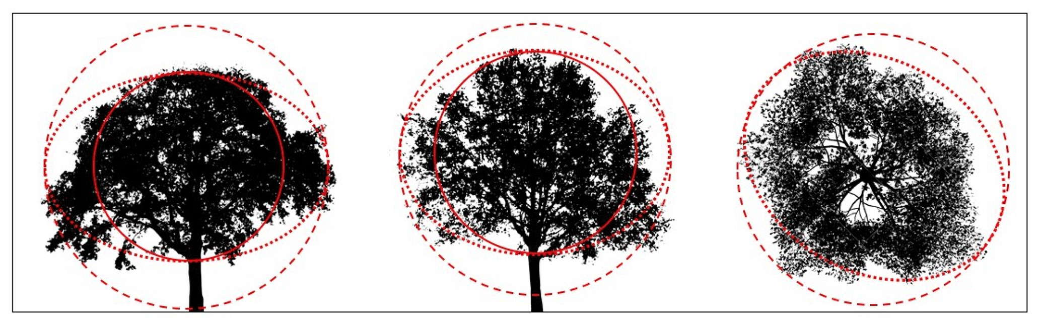
Figure 2 Illustration of various crown envelope definitions applied to three different trees (two side view, one top view). The solid line is a sphere based on the vertical extent of the crown, the dashed line is a sphere based on the horizontal extent of the crown, and the dotted line is an ellipsoid based on the horizontal and vertical extent of the crown.

3 Test case setup

3.1 Overview

While it is possible to test the above modeling framework using field data, this approach is severely limited by the lack of systematic variation in canopy architecture as well as experimental errors that can become convoluted with model errors. As such, it can be difficult if not impossible to use field data to rigorously evaluate and diagnose issues within models. In this work, an alternative approach was used to evaluate model performance, which was based on the use of a detailed 3-D leaf-resolving model to simulate radiation absorption in virtually generated canopies. The advantage of this approach is that arbitrary canopy geometries can be generated in which the exact geometry is known, which provides the necessary inputs for a 1-D model. The limitation of course is that results are confined within the assumptions and accuracy inherent in the chosen 3-D model. In order to minimize this limitation, the ray-tracing-based model of Bailey (2018) was used as implemented in the Helios 3-D modeling framework (Bailey, 2019). Provided that simulated surfaces are isotropic absorbers, Bailey (2018) showed that this model converges exponentially toward the exact solution as the number of rays is increased. It has also been shown to converge to the solution given by Beer's law for a truly homogeneous canopy (Ponce de León and Bailey, 2019). Since it was verified that further increasing the number of rays did not significantly affect results, we considered the 3-D model solution to be the reference or exact solution against which the various 1-D models could be compared. The canopy-level intercepted radiation flux was calculated from the 3-D model output as

$$\begin{array}{}\text{(17)}& P={\displaystyle \frac{\mathrm{1}}{R_{\downarrow }{A}_g}}\sum _{i=\mathrm{1}}^{N_p}{R}_i{A}_i,\end{array}$$

where R_↓ is the above-canopy solar radiation flux on a horizontal surface, A_g is the horizontal area of the canopy footprint, R_i is the radiative flux incident on the ith of N_p total vegetative elements, and A_i is the one-sided surface area of the ith vegetative element.

A number of test cases were formulated to progressively test different aspects of each of the models given in Table 2. For each of the test cases below, all surfaces were black, and the ambient diffuse radiation flux was set to zero in order to maintain consistency with these non-geometric assumptions inherent in Beer's law. The above-canopy solar radiation flux was modeled using the REST-2 model (Gueymard, 2003). The model was run at an hourly time step for Julian day 79, and the position on the earth was the Equator. This date and location were chosen because a single diurnal cycle provides a full range of solar zenith angles ranging from 0 to π∕2. This means that it is not explicitly necessary to evaluate performance under diffuse conditions because, as was illustrated by Eq. (15), the diffuse radiation flux is simply a weighted average of the flux originating from all zenithal directions.

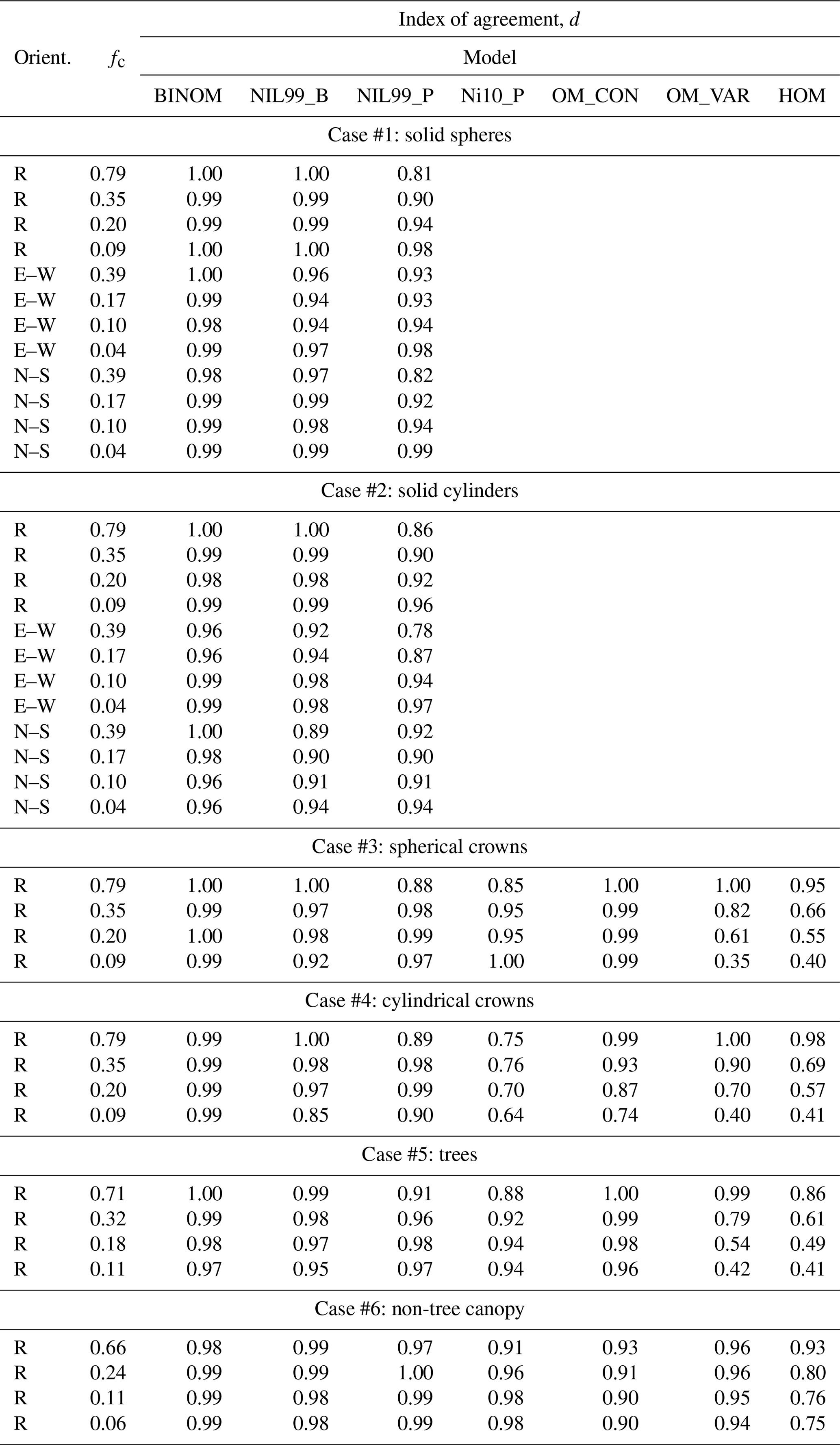
Agreement between each of the 1-D models and the 3-D model were analyzed graphically and quantitatively using the index of agreement (Willmott, 1981), which is defined mathematically as

$$\begin{array}{}\text{(18)}& d=\mathrm{1}-{\displaystyle \frac{\sum _{i=\mathrm{1}}^{N_t}{\left(O_i-M_i\right)}^{\mathrm{2}}}{\sum _{i=\mathrm{1}}^{N_t}{\left(|O_i-\stackrel{\mathrm{‾}}{O}|+|M_i-\stackrel{\mathrm{‾}}{M}|\right)}^{\mathrm{2}}}},\end{array}$$

where O_i is the ith of N_t flux values from the 3-D model (reference dataset), M_i are flux values predicted by the 1-D model, and an overbar denotes an average over all N_t values.

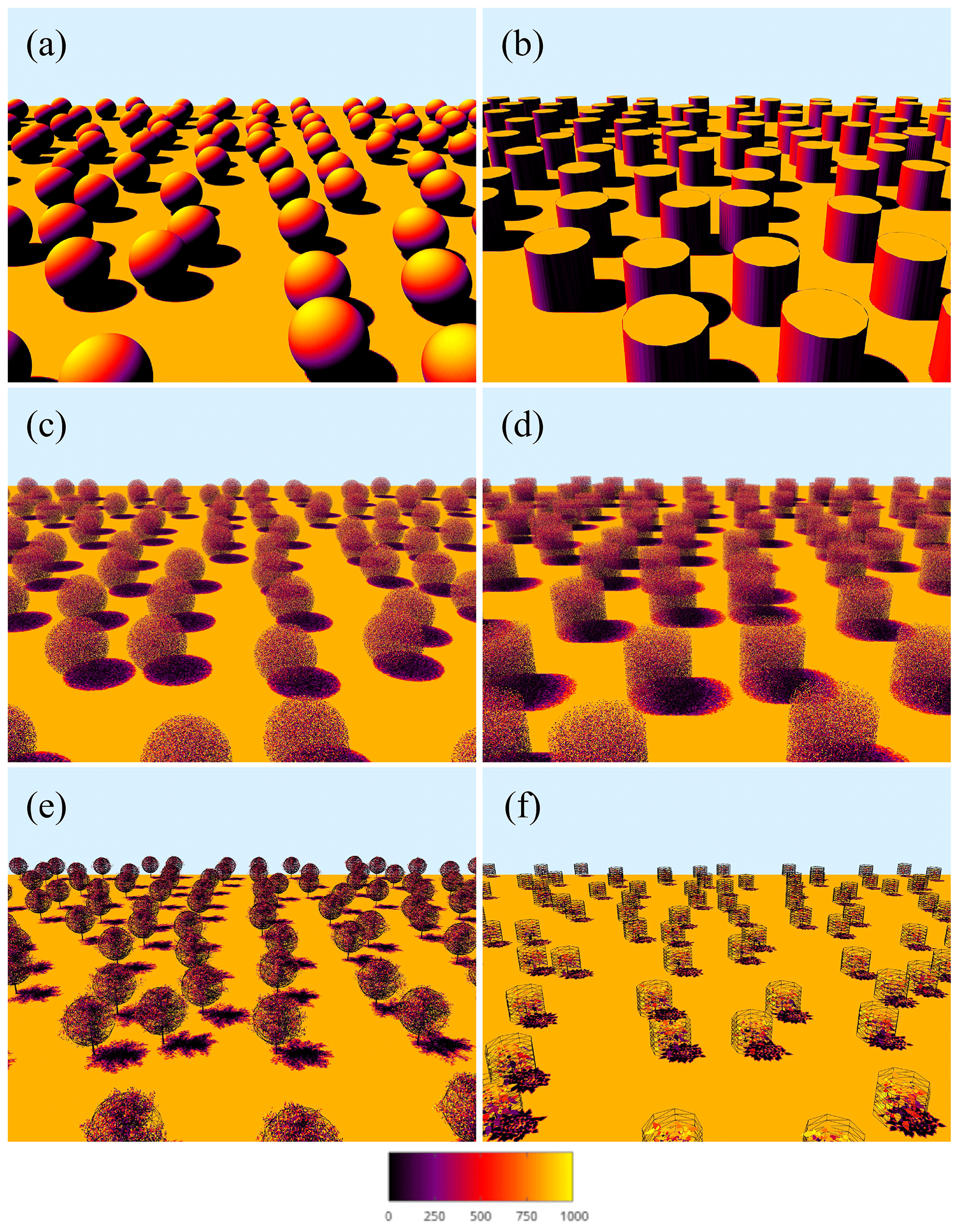
Figure 3 Visualization of virtual canopy geometries: (a) Case #1 – solid spheres, (b) Case #2 – solid cylinders, (c) Case #3 – uniform vegetation in spherical crowns, (d) Case #4 – uniform vegetation in cylindrical crowns, (e) Case #5 – tree canopy, and (f) Case #6 – non-tree plant canopy (potato). Wireframe meshes in (e) and (f) show the assumed crown envelope based on a best fit to the exact radiation interception. Surfaces are colored using a pseudocolor mapping of the modeled intercepted radiation flux (W m⁻²).

3.2 Case #1: canopy of solid spheres

In order to isolate the effects of crown-scale clumping, a test case was considered in which the canopy consisted of solid, opaque spheres of radius R=5 m with varying spacing (Fig. 3a). In the first configuration, spheres were arranged randomly with an average spacing in the horizontal direction of s∕R = 2, 3, 4, and 6. It should be noted that the placement of spheres was not truly random, as crowns were not allowed to overlap. The second configuration placed the spheres in a nonrandom row orientation in which the plant spacing in the row-parallel direction was s_p∕R = 2, 3, 4, and 6, and the row spacing was s_r∕R = 4, 6, 8, and 12. Rows were oriented in either the north–south or east–west directions, and crowns were not allowed to overlap. The spheres were positioned on the ground surface, and thus the canopy height was h=2R. The 1-D models were evaluated with L=∞ since the spheres were solid. Only the models BINOM, NIL99_B, and NIL99_P were considered for this case because they separately account for crown and sub-crown intersection.

3.3 Case #2: canopy of solid cylinders

To test generalization to geometries with anisotropic crowns, a case was considered with a canopy of solid, opaque cylinders of radius R=5 m and height H=2R (Fig. 3b). The setup was essentially the same as Case #1, with random, north–south and east–west arrangements of crowns with the same set of spacings.

3.4 Case #3: canopy of uniformly distributed leaves in spherical crowns

In order to test the combined effects of crown-scale clumping and leaf-scale attenuation, a test case was considered in which the canopy consisted of spherical crowns containing homogeneous and isotropic vegetation elements (Fig. 3c). Spherical crowns of radius R=5 m were generated in which rectangular leaves of size 0.1 m×0.1 m were arranged randomly inside the crown with a uniform spatial distribution and were randomly oriented following a spherical distribution (G=0.5). For brevity, only the random crown arrangement is presented, which had the same average spacing as in Case #1 above. The leaf area density within each crown was set at $a=\mathrm{0.5}{\mathrm{m}}^{-\mathrm{1}}$, and the whole-canopy LAI can be calculated as $L={\displaystyle \frac{\mathrm{4}\mathit{\pi }{R}^{\mathrm{3}}a}{\mathrm{3}{s}^{\mathrm{2}}}}$, which gives LAI values ranging from 0.3 to 2.6.

3.5 Case #4: canopy of uniformly distributed leaves in cylindrical crowns

Similar to Case #3, an additional case was considered consisting of cylindrical crowns of radius R=5 m and H=2R, filled with uniformly distributed leaves (Fig. 3d). All other parameters are the same as Case #3. For cylindrical crowns, the whole-canopy LAI is $L={\displaystyle \frac{\mathit{\pi }{R}^{\mathrm{2}}Ha}{s^{\mathrm{2}}}}$, which gives LAI values ranging from 0.44 to 3.9.

3.6 Case #5: canopy of trees

In order to test the models for more realistic canopy architectures, canopies of trees were constructed using the procedural tree generator of Weber and Penn (1995) (Fig. 3e) as implemented in the Helios 3-D modeling framework (Bailey, 2019). The trunk and branches consisted of a triangular mesh of elements forming cylinders, and leaves were rectangles of size 0.12 m×0.03 m that were masked into the shape of a leaf using the transparency channel of a PNG image of a leaf (see Bailey, 2019). The tree crown envelope was approximately spherical in shape, but the spatial distribution of leaves was nonuniform. Leaf angles were sampled from a spherical distribution, and thus G=0.5. Note that in calculating radiation interception, a distinction was not made between branches or leaves, but rather total attenuation was used. The tree height was approximately h=6.5 m, and trees were randomly arranged with average spacing in the horizontal direction of s=5, 7.5, 10, 15, and 20 m. The canopy leaf area index values were L=3.86, 1.57, 0.97, 0.39, and 0.24. An effective crown radius was estimated to be R=2.9 m, which was the value that gave the best predictions of radiation interception at a solar zenith angle of zero. Figure 3e shows a visualization of the assumed crown envelope based on a best fit of both the BINOM and NIL99_BINOM models to the exact intercepted flux. The leaf area density was variable in space, and thus an effective density within the crown was substituted into the 1-D equations, which was calculated as $a={\displaystyle \frac{\mathrm{3}L{s}^{\mathrm{2}}}{\mathrm{4}\mathit{\pi }{R}^{\mathrm{3}}}}$.

3.7 Case #6: canopy of non-tree plants

A potato plant canopy was generated to test the models in more realistic non-tree canopies (Fig. 3f). Similar to the tree canopies, the stem consisted of a mesh of triangles, and leaves were texture-masked rectangles. The crown envelope could be considered roughly cylindrical, with leaves of variable size distributed nonuniformly within the cylinder. The leaf angle distribution was highly anisotropic, with G ranging from 0.87 when the sun direction was vertical to 0.23 when the sun direction was horizontal. The effective dimensions of the crown envelope were estimated to be R=0.5 m and H=0.75 m, which is visualized in Fig. 3f. Plants were arranged randomly, where the average plant spacing was s=1.2, 2, 3, 4 m. The canopy leaf area index values were L=0.67, 0.24, 0.11, 0.061. The effective crown leaf area density was estimated as $a={\displaystyle \frac{L{s}_{\text{p}}{s}_{\text{r}}}{\mathit{\pi }{R}^{\mathrm{2}}H}}$.

Table 3 Summary of test case results. Agreement between the four models of radiation interception is compared against the exact interception using the index of agreement (Eq. 18).

4 Results

4.1 Case #1: canopy of solid spheres

Figure 4 gives time series of the exact intercepted radiation flux compared against the simplified 1-D models for each of the canopies of solid spheres with four densities and three plant arrangements. For random plant arrangement (Fig. 4a–d), the binomial models performed very well for all ground cover fractions, with the best performance occurring at the highest plant density of f_c=0.79 (d≈1.0). The Poisson model significantly underpredicted the intercepted flux for most zenith angles, with the underprediction being largest at θ=0. The performance of the Poisson model improved as the canopy became less dense, such that its performance was near that of the binomial model for the sparsest case of f_c=0.09.

For the east–west, row-oriented configuration (Fig. 4e–h), performance of the BINOM model was nearly the same as in the randomly oriented case. As would be expected, the performance of the NIL99_B model decreased in the east–west, row-oriented case as it assumes an azimuthally symmetric distribution of crowns (e.g., d decreased from about 1.0 to 0.94 in the sparsest case). The performance of the Poisson model (NIL99_P) actually increased slightly for the east–west orientation – however this is likely the result of offsetting errors. As evidenced by the NIL99_B results, an east–west row orientation appeared to cause an overprediction of the intercepted flux, which offsets some of the underprediction due to the assumption of a Poisson distribution in the probability of crown intersection.

Overall, the BINOM model performed equal to or better than the NIL99_B and NIL99_P models for every canopy configuration. The lowest d value for the BINOM, NIL99_B, and NIL99_P models, respectively, was 0.98, 0.94, and 0.81. It is noted that for the case of a canopy of solid objects with random spacing, the BINOM and NIL99_B models are mathematically equivalent, which is confirmed by the results.

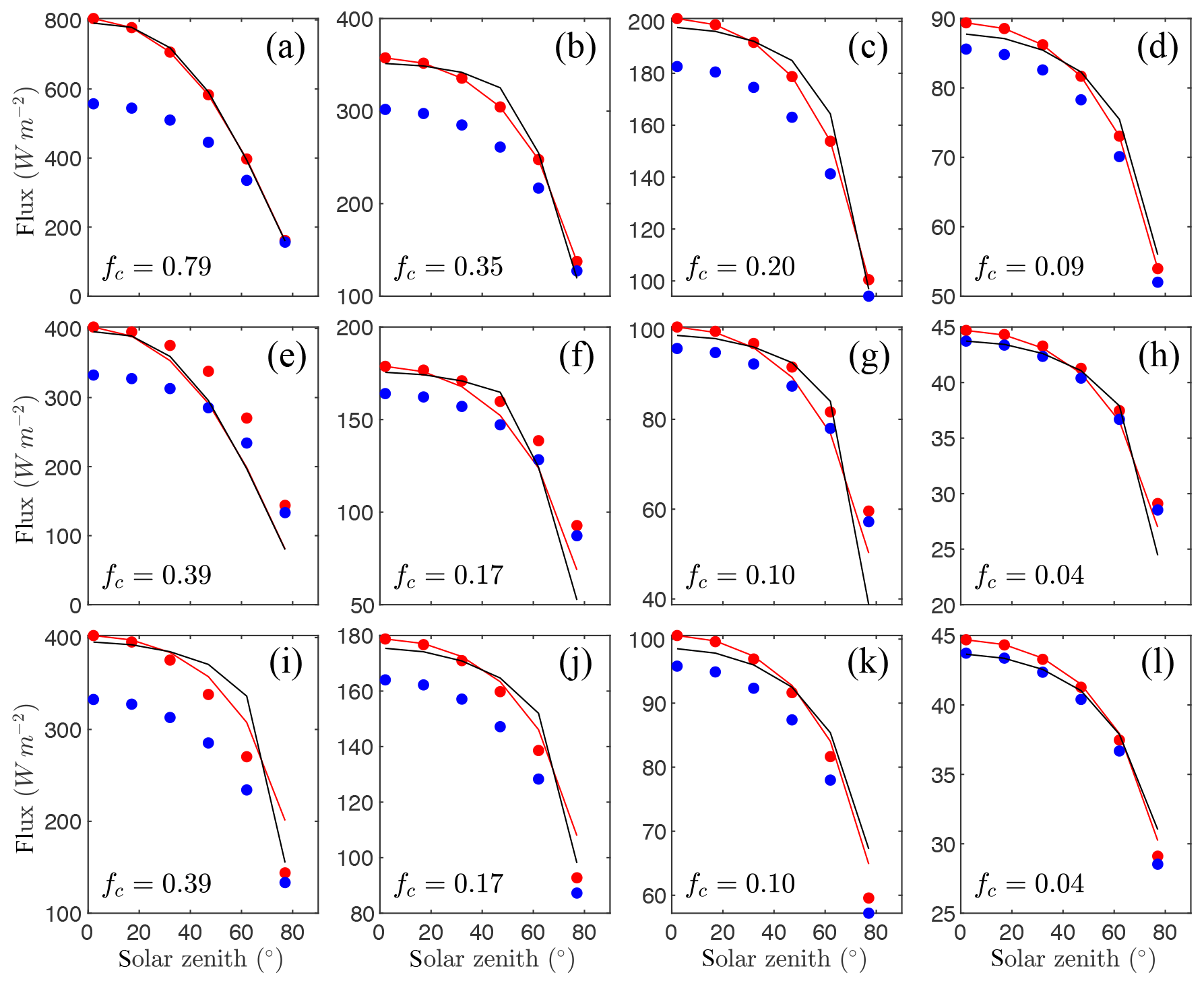
Figure 4 Flux of intercepted radiation versus solar zenith angle for a half-diurnal cycle in a canopy of solid spheres (see Fig. 3a). Varying ground cover fractions f_c were simulated (rows in figure) for three different plant arrangements: (a–d) randomly spaced, (e–h) east–west row orientation, and (i–l) north–south row orientation. The exact flux is given by the output of the 3-D model (black line), which is compared against the 1-D models BINOM (red line), NIL99_B (red circle), and NIL99_P (blue circle).

4.2 Case #2: canopy of solid cylinders

Figure 5 gives time series of the exact intercepted radiation flux compared against the simplified 1-D models for each of the canopies of solid cylinders with four different densities and three plant arrangements. Trends in model performance were similar as in the solid sphere case (Fig. 4), except that overall performance for all models was decreased slightly. The lowest d value for the BINOM, NIL99_B, and NIL99_P models, respectively, was 0.96, 0.89, and 0.78. Again, the BINOM model performed exactly equal to the NIL99_B model, and consistently outperformed the NIL99_P model.

Figure 5 Flux of intercepted radiation versus solar zenith angle for a half-diurnal cycle in a canopy of solid cylinders (see Fig. 3b). Varying ground cover fractions f_c were simulated (rows in figure) for three different plant arrangements: (a–d) randomly spaced, (e–h) east–west row orientation, and (i–l) north–south row orientation. The exact flux is given by the output of the 3-D model (black line), which is compared against the 1-D models BINOM (red line), NIL99_B (red circle), and NIL99_P (blue circle).

4.3 Case #3: canopy of uniformly distributed leaves in spherical crowns

Figure 6 gives time series of the exact intercepted radiation flux compared against the simplified 1-D models for each of the canopies of randomly spaced spherical crowns with four different average densities. The BINOM model performed very well for all densities, with d≥0.99. Performance of NIL99_B was worse than BINOM for this case, as NIL99_B assumes that the radiation path length is constant across the crown cross section. This assumption had essentially no impact in the densest planting density but decreased d from 0.99 to 0.92 in the sparsest case. The Poisson models (NIL99_P and NI10_P) showed similar underprediction as in Case #1 (solid spheres), indicating that most of the error originates from the assumption of a Poisson distribution. The primary difference between the NIL99_P and NI10_P models is that the NIL99_P model assumes the radiation path length is constant across the crown cross section, which caused a slight increase in the intercepted flux for NIL99_P (as was the case for the NIL99_B versus BINOM models).

The OM_VAR model had very large errors as the canopy became increasingly sparse. For zenith angles near 90^∘, this model had an overprediction as large as the homogeneous model, which decreased toward that of the other models as zenith angle decreased. It should be noted that the OM_VAR is forced to match the exact flux perfectly at θ=0, and it only needs to model the flux for θ>0. The OM_CON model, which also is forced to perfectly match the exact flux at θ=0, performed as well as the BINOM model (d≥0.99). This model, which assumes a constant impact of heterogeneity for θ>0, performed much better than the OM_VAR model. Such a result is to be expected, given that for spherical crowns, the crown envelope as well as leaf orientation is isotropic. Thus, since Ω(θ) is dependent on both the impact of heterogeneity and G(θ), the fact that both G and the heterogeneity are approximately constant means that Ω is approximately constant.

Figure 6 Flux of intercepted radiation versus solar zenith angle for a half-diurnal cycle in a canopy of spherical crowns filled with uniformly distributed leaves (see Fig. 3c). Varying ground cover fractions f_c were simulated as labeled in each pane. The exact flux is given by the output of the 3-D model (black line), which is compared against the 1-D models BINOM (red line), NIL99_B (red circle), and NIL99_P (blue circle) and Ni10_P (blue line), OM_CON (black circle), OM_VAR (green triangle), and HOM (dotted line).

4.4 Case #4: canopy of uniformly distributed leaves in cylindrical crowns

Figure 7 gives time series of the exact intercepted radiation flux compared against the simplified 1-D models for each of the canopies of randomly spaced cylindrical crowns with four different average densities. The anisotropic crown shape acted to better distinguish between the models than did the spherical crown shapes. The BINOM model performed very well for all planting densities (d≥0.99). As in the case of the solid cylinder canopy, the assumption of constant crown path length resulted in a slight overprediction of the NIL99_B model, which appeared to increase as the canopy became increasingly sparse. Both of the Poisson models (NIL99_P and NI10_P) significantly underpredicted the intercepted flux in the densest canopy case. For the sparsest case, the Poisson model NI10_P still significantly underpredicted the flux, whereas NIL99_P overpredicted the flux.

The OM_VAR model had a very large overprediction of radiation interception at high zenith angles, as in the spherical crown case. Unlike in the spherical crown case, the OM_CON model did not perform well, particularly as the canopy became increasingly sparse. When crowns are cylindrical, heterogeneity is no longer isotropic, especially as the plant spacing becomes large and as such interception varies irregularly with θ. As a result, Ω has strong θ dependence and cannot be assumed constant.

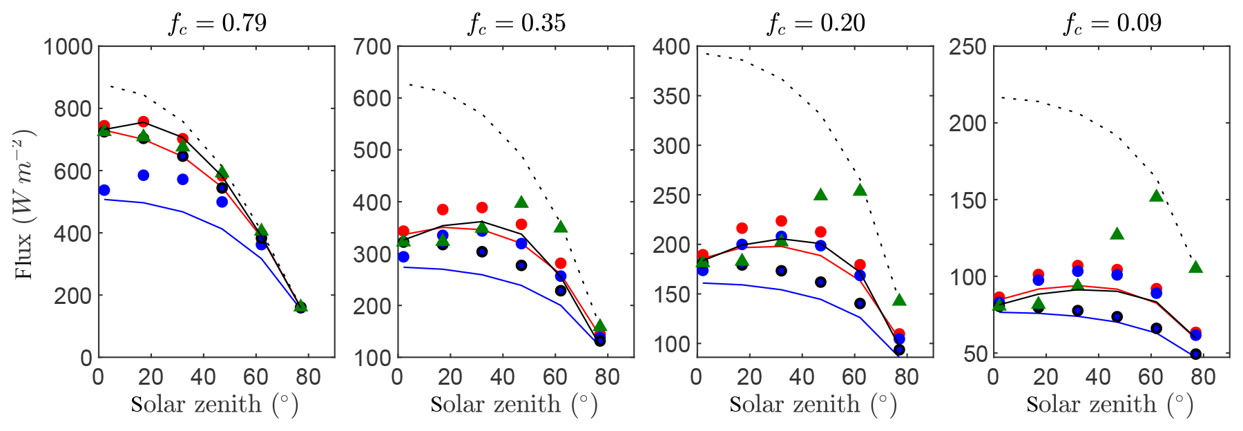
Figure 7 Flux of intercepted radiation versus solar zenith angle for a half-diurnal cycle in a canopy of cylindrical crowns filled with uniformly distributed leaves (see Fig. 3d). Varying ground cover fractions f_c were simulated as labeled in each pane. The exact flux is given by the output of the 3-D model (black line), which is compared against the 1-D models BINOM (red line), NIL99_B (red circle), and NIL99_P (blue circle), Ni10_P (blue line) and OM_CON (black circle), OM_VAR (green triangle), and HOM (dotted line).

4.5 Case #5: canopy of trees

Figure 8 gives time series of the exact intercepted radiation flux compared against the simplified 1-D models for each of the canopies of randomly spaced trees with four different average densities. Results were quite similar to that of Case #3 (spherical crowns). Model agreement with the reference intercepted flux was reduced slightly overall for each of the models, which is likely due to the fact that the assumptions of spherical crown shape and within-crown homogeneity were not exactly satisfied. However, this reduction in performance was small, and the BINOM model still performed very well. Thus, this test confirms generalizability to more realistic tree architectures in which vegetation within the crown envelope is only approximately homogeneous and the crown shape is only approximately spherical.

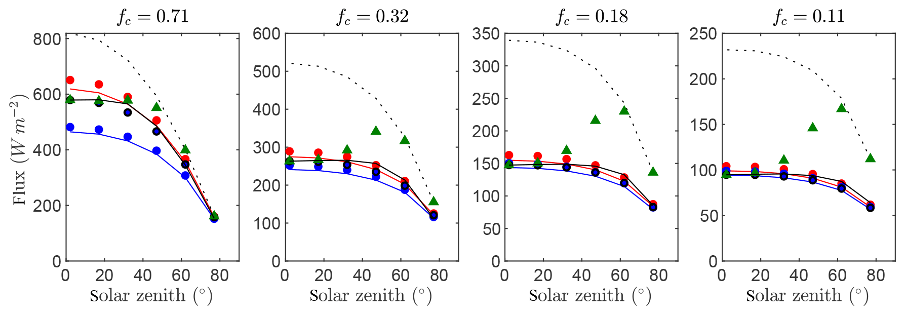
Figure 8 Flux of intercepted radiation versus solar zenith angle for a half-diurnal cycle in a canopy of trees (see Fig. 3e). Varying ground cover fractions f_c were simulated as labeled in each pane. The exact flux is given by the output of the 3-D model (black line), which is compared against the 1-D models BINOM (red line), NIL99_B (red circle), and NIL99_P (blue circle) and Ni10_P (blue line), OM_CON (black circle), OM_VAR (green triangle), and HOM (dotted line).

4.6 Case #6: non-tree canopy

Figure 9 gives time series of the exact intercepted radiation flux compared against the simplified 1-D models for each of the canopies of randomly spaced non-tree plants (potato) with four different average densities. Results were also similar to the canopy with cylindrical crowns (Case #4), with only slightly reduced overall performance in comparison to Case #4. It is noted that this was the only case with an anisotropic leaf angle distribution, but the high anisotropy in G did not seem to significantly affect model performance.

Figure 9 Flux of intercepted radiation versus solar zenith angle for a half-diurnal cycle in a canopy non-tree plants (potato; see Fig. 3f). Varying ground cover fractions f_c were simulated as labeled in each pane. The exact flux is given by the output of the 3-D model (black line), which is compared against the 1-D models BINOM (red line), NIL99_B (red circle), and NIL99_P (blue circle) and Ni10_P (blue line), OM_CON (black circle), OM_VAR (green triangle), and HOM (dotted line).

5 Discussion

The simplest models, based on an Ω clumping factor that effectively scales the attenuation coefficient, had mixed success depending on the particular case. Assuming a constant Ω factor (OM_CON model) worked quite well in the case that the heterogeneity (crowns) was roughly isotropic. As mentioned previously, Ω encapsulates the effects of G(θ), heterogeneity, and the apparent LAI that results from the heterogeneity to form an inseparable product G Ω L. If this product is isotropic, then it is reasonable to assume a constant Ω. The problem, however, is still that this constant Ω is not known a priori and must be determined from radiation measurements at a particular solar zenith angle (preferably near θ=0) in order to invert for the appropriate attenuation coefficient.

The OM_VAR model (Campbell and Norman, 1998) attempts to model the effects of anisotropic clumping for θ>0. When the canopy was fairly dense, the OM_VAR model worked fairly well. However, the OM_CON and HOM models generally performed as well or better than the OM_VAR model for those cases, and thus there is no reason to use a variable Ω factor. As the canopy became increasingly sparse, the performance of the OM_VAR model declined significantly and overpredicted interception as the solar zenith angle increased (note that this model also forces the predicted flux to match the reference flux exactly at θ=0). Kucharik et al. (1999) evaluated the framework behind the OM_VAR model in a number of different canopies and found that it was able to fit the data well but that the model coefficients were highly species specific. One issue with their validation approach, which is symptomatic of many field validation studies of heterogeneous canopy radiation models, is that the data were collected in relatively dense canopies where heterogeneity is fairly low overall. The canopies studied in Kucharik et al. (1999) had a ground cover fraction approximately in the range of f_c=0.5–0.75, which would place them on the denser end of the canopy cases considered in the present study, which is where the OM_VAR model worked well. However, it was shown that for these cases a constant Ω factor model (OM_CON) or even the homogeneous model (HOM) also worked well.

The assumption that the probability of intersecting a crown envelope follows a Poisson distribution did not work well unless the canopy was very sparse. For most canopy densities, the Poisson models significantly underpredicted the absorbed flux. It appeared that when the mean free path of radiation propagation (which is related to the crown spacing) was not significantly smaller than the actual radiation propagation distance through the canopy (which is related to the canopy height and solar zenith), the assumption of a Poisson distribution was poor. The Poisson distribution assumes that the canopy consists of a large number of “layers” of randomly positioned elements. When the solar zenith angle is near vertical, the canopy consists of a single layer of crowns. For solid spherical crowns, the probability of interception should be f_c at θ=0, but with the Poisson model it is $\mathrm{1}-\exp (-f_{\text{c}})$, which is always less than f_c. As f_c approaches zero, $\mathrm{1}-\exp (-f_{\text{c}})\approx f_{\text{c}}$, which is demonstrated by the results of the Poisson model (NI10_P and NIL99_P) evaluation. The NI10_P model has been validated against experimental data by Yang et al. (2010), which showed relatively good model performance. All of the experimental canopies in Yang et al. (2010) were quite dense with high LAI and ground cover fraction. As illustrated previously, specification of the crown radius can be ambiguous for real trees that are irregularly shaped. If the crown radius is specified based on an envelope encapsulating all branches, this effectively inflates R and f_c, which would presumably result in an overprediction of the intercepted flux. However, this overprediction could be offset by applying a Poisson model, which was shown to cause underprediction. It is possible that R was inflated in Yang et al. (2010) (which considered only dense canopy cases), and offsetting errors associated with the Poisson assumption resulted in artificially improved model performance due to offsetting errors. The crown radius in Case #2 is exactly known, so specification of R in that case is not a potential source of model error. In another study, the NI10_P model was compared against other models for a set of virtual canopies where the exact geometry was known (but the exact radiation interception was not), which suggested that the NI10_P model tended to predict higher canopy transmission (lower interception) than the other models (Widlowski et al., 2013), which is also consistent with the results of the present study.

The assumption that crown intersection followed a binomial distribution appeared to hold for all canopy cases considered in this work. The binomial model predicts the correct interception at θ=0, which corresponds to a single crown layer (N_c=1) and P=f_c, rather than $P=\mathrm{1}-\exp (-f_{\text{c}})$ in the case of the Poisson model. The BINOM model outperformed all other models for every test considered. The primary difference between the formulation of BINOM and NIL99_B is that (1) the NIL99_B model assumes that the path length of radiation through an individual crown is constant, whereas the BINOM model accounts for variable path length, and (2) the NIL99_B model assumes that crowns are randomly positioned in space and thus that crown intersection is azimuthally symmetric, whereas the BINOM model accounts for asymmetry. The assumption of constant path lengths created modest errors, as evidenced by the results of Cases #3 and #4. The assumption of random positioning of crowns in a row-oriented canopy had the potential to create very large errors, as evidenced by the results of Cases #1 and #2. These errors are caused by the fact that the effective total path length through vegetation in a row-oriented canopy can change significantly with azimuth.

The scope of the results of this study are clearly limited to cases of no scattering and no diffuse radiation. These impacts were excluded from the study to focus on cases where, aside from heterogeneity in the geometry, the assumptions of Beer's law should be exactly satisfied. Although Beer's law is only valid along a single direction of radiation propagation, and its derivation requires the removal of scattering terms in the RTE, variations have been derived that approximate the effects of scattering and diffuse radiation within a 1-D model (e.g., Lemeur and Blad, 1974; Goudriaan and Van Laar, 1994).

It appears likely that many crop models, global ecosystem models, and land surface models overestimate radiation interception by applying the homogeneous Beer's law in heterogeneous environments, which is sure to have important consequences for large-scale flux estimates. Incorporation of the results of this work within these models is straightforward and requires specification of either the ground cover fraction f_c or the planting density and effective crown envelope. Algorithms are readily available for separation of the ground surface and vegetation within aerial images in order to calculate the ground cover fraction (e.g., Gougeon, 1995; Luscier et al., 2006; Laliberte et al., 2007). The results of Cases #5 and #6 suggested that rough estimations of the crown envelope dimensions based on visual inspection could yield reasonable results.

6 Conclusions

Simplified models of radiation interception in heterogeneous canopies can be readily derived by separating the canopy into hierarchical scales of clumping over which the probability of interception can be assumed homogeneous in space over some discrete volume. The results of this work demonstrated that very good predictions of whole-canopy interception can be achieved using simple geometric models that consider only crown-scale and leaf-scale clumping (in the absence of scattering). The probability of intersecting a plant crown was well represented by a (positive) binomial distribution. This model calculates the probability of not intersecting a leaf within a single crown and compounds this probability N_c times, where N_c is the number of crowns a given beam of radiation traverses on its path from the top to the bottom of the canopy. The Poisson models for crown intersection did not perform well unless the canopy was fairly dense, but in this case the effects of heterogeneity are less important, and the homogeneous Beer's law also performs well. The results of the model evaluation exercise confirm that the binomial model given in Eq. (13) (BINOM) is the preferable model in all cases considered herein. Inputs to the model can be specified based on measurements of plant geometry or through inversion if radiation interception measurements are available for a particular solar zenith angle.

Appendix A: Descriptions of previously proposed models

For completeness, model equations taken from the literature are provided below as they were implemented and using the notation adopted in this paper.

A1 Model of Nilson (1999): NIL99_B and NIL99_P

Assuming that the probability of intersecting a crown envelope follows a (positive) binomial distribution, Nilson (1999) gives the probability of intersection for a canopy to be

$$\begin{array}{}\text{(A1)}& P=\mathrm{1}-{\left(\mathrm{1}-(\mathrm{1}-P_{\mathrm{1}})S\left(\mathrm{0}\right)/s^{\mathrm{2}}\right)}^{N_{\text{c}}},\end{array}$$

where $N=S\left(\mathit{\theta }\right)/S\left(\mathrm{0}\right)$, S(θ) is the area of the crown envelope shadow, S(0) is the area of the crown envelope shadow at a solar zenith angle of zero, s is the mean plant spacing, and P₁ is the probability that a beam of radiation does not intersect a leaf within a single crown and is given by

$$\begin{array}{}\text{(A2)}& P_{\mathrm{1}}=\exp \left(-{\displaystyle \frac{G\left(\mathit{\theta }\right)L{s}^{\mathrm{2}}}{S\left(\mathit{\theta }\right)\cos \mathit{\theta }}}\right).\end{array}$$

If the probability of intersecting a crown envelope is instead assumed to follow a Poisson distribution, Nilson (1999) gives the probability of intersection for a canopy to be

$$\begin{array}{ll}{\displaystyle }P=& {\displaystyle }\mathrm{1}-\exp \left(-{\displaystyle \frac{S\left(\mathrm{0}\right)}{s^{\mathrm{2}}}}(\mathrm{1}-P_{\mathrm{1}})N_{\text{c}}\right)\\ \text{(A3)}& {\displaystyle }=& {\displaystyle }\mathrm{1}-\exp \left(-{\displaystyle \frac{S\left(\mathit{\theta }\right)}{s^{\mathrm{2}}}}(\mathrm{1}-P_{\mathrm{1}})\right).\end{array}$$

There are two notable differences between Eq. (13) and the model of Nilson (1999). The first was mentioned above, which is that the expression for N_c in Nilson (1999) assumes a random or uniform spatial distribution of crowns, whereas Eq. (13) has been generalized to include row-oriented crowns. Second is that Nilson (1999) assumed a spatially constant within-crown path length in calculating P₁, whereas P_ℓ accounts for variable beam path lengths through crowns (Eq. 10).

A2 Model of Campbell and Norman (1998): OM_VAR

Kucharik et al. (1997) originally suggested a simple empirical model describing the θ dependence of Ω, provided that the value of Ω at θ=0 is known,

$$\begin{array}{}\text{(A4)}& \mathrm{\Omega }\left(\mathit{\theta }\right)={\displaystyle \frac{\mathrm{\Omega }\left(\mathrm{0}\right)}{\mathrm{\Omega }\left(\mathrm{0}\right)+\left(\mathrm{1}-\mathrm{\Omega }\left(\mathrm{0}\right)\exp \left(-k{\mathit{\theta }}^p\right)\right)}},\end{array}$$

where Ω(0) is the value of Ω when the solar zenith angle is zero, and k and p are geometric coefficients with p given by (Campbell and Norman, 1998)

$$\begin{array}{}\text{(A5)}& p=\mathrm{3.8}-\mathrm{0.46}D,\mathrm{1}\le p\le \mathrm{3.34},\end{array}$$

where D is the ratio of the crown depth to the crown diameter. The coefficient k is taken to be equal to 2.2 as suggested by Campbell and Norman (1998).

An obvious limitation of this approach is that the value of Ω(0) must be estimated, which usually requires midday solar interception data. It does, however, make modeling easier since this approach guarantees that the correct radiation interception will be predicted around midday.

A3 Model of Ni-Meister et al. (2010): NI10_P

Ni-Meister et al. (2010) suggested a geometric model based on spherical crowns, which is an analytical form of the model originally proposed by Li and Strahler (1988). Their approach used geometry of spheres to back calculate the appropriate clumping factor Ω, which is given by

$$\begin{array}{}\text{(A6)}& \mathrm{\Omega }={\displaystyle \frac{\mathrm{3}}{\mathrm{4}{\mathit{\tau }}_{\mathrm{0}}r}}\left(\mathrm{1}-{\displaystyle \frac{(\mathrm{1}-(\mathrm{2}{\mathit{\tau }}_{\mathrm{0}}r+\mathrm{1}\left)\exp \left(-\mathrm{2}{\mathit{\tau }}_{\mathrm{0}}r\right)\right)}{\mathrm{2}({\mathit{\tau }}_{\mathrm{0}}r{)}^{\mathrm{2}}}}\right),\end{array}$$

where

$$\begin{array}{}\text{(A7)}& {\mathit{\tau }}_{\mathrm{0}}r={\displaystyle \frac{\mathrm{3}G\left(\mathit{\theta }\right)L}{\mathrm{4}\mathit{\lambda }\mathit{\pi }{R}^{\mathrm{2}}}},\end{array}$$

and recalling that G is the fraction of leaf area projected in the direction of radiation propagation, L is the canopy leaf area index, λ is the number of plants per unit ground area, and R is the crown radius.

Since Ni-Meister et al. (2010) formulated their model in terms of an Ω clumping factor, the end equations for the models of Ni-Meister et al. (2010) and Nilson (1999) look quite different. However, mathematically they are nearly the same. The primary difference in the formulation is that Nilson (1999) assumes a constant effective path length through crowns in calculating the probability of leaf intersection, whereas Ni-Meister et al. (2010) explicitly calculates the weighted average probability based on variable path lengths.