the Creative Commons Attribution 4.0 License.
the Creative Commons Attribution 4.0 License.
 | 02 Oct 2020
Role of atmospheric horizontal resolution in simulating tropical and subtropical South American precipitation in HadGEM3-GC31
Amulya Chevuturi
Peter Cook
Nicholas P. Klingaman
Christopher E. Holloway
We assess the effect of increasing horizontal resolution on simulated precipitation over South America in a climate model. We use atmosphere-only simulations, performed with HadGEM3-GC31 at three horizontal resolutions: N96 (∼130 km; ), N216 (∼60 km; ), and N512 (∼25 km; ). We show that all simulations have systematic biases in annual mean and seasonal mean precipitation over South America (e.g. too wet over the Amazon and too dry in the northeast). Increasing horizontal resolution improves simulated precipitation over the Andes and northeast Brazil. Over the Andes, improvements from horizontal resolution continue to ∼25 km, while over northeast Brazil, there are no improvements beyond ∼60 km resolution. These changes are primarily related to changes in atmospheric dynamics and moisture flux convergence. Over the Amazon Basin, precipitation variability increases at higher resolution. We show that some spatial and temporal features of daily South American precipitation are improved at high resolution, including the intensity spectra of rainfall. Spatial scales of daily precipitation features are also better simulated, suggesting that higher resolution may improve the representation of South American mesoscale convective systems.
- Article
(15354 KB) - Full-text XML
-
Supplement
(4601 KB) - BibTeX
- EndNote


South America is a large area encompassing tropical, sub-tropical, and extratropical climates. The Andes cover western South America, from south to north, while the eastern part of South America is flatter than the west. The Amazon Basin has high mean rainfall and is covered by a rainforest, while northeastern Brazil is semi-arid. Several climatic areas are thus often defined to account for the climatic heterogeneity of South America, with a focus specifically on the Andes, the Amazon Basin, northeast Brazil, and southeast Brazil (Custodio et al., 2017).
Climate models have biases in simulating South American precipitation, partly due to biases in simulating teleconnections between both Atlantic and Pacific sea-surface temperatures (SSTs), and precipitation over land (Bombardi and Carvalho, 2008; Coelho et al., 2016; Jung et al., 2011; Koutroulis et al., 2016; Sierra et al., 2015; Yin et al., 2013). At sub-seasonal scales, precipitation variability is associated with the Madden–Julian oscillation (MJO) (Grimm, 2019). The MJO modulates precipitation over South America, leading to either anomalously dry or wet conditions, depending on its phase. The MJO also favours extreme events, leading to droughts and floods (Grimm, 2019). At interannual scales, the El Niño–Southern Oscillation (ENSO) strongly impacts Amazon precipitation, with El Niño events related to droughts (Grimm and Silva Dias, 1995; Grimm and Tedeschi, 2009; Lewis et al., 2011; Marengo et al., 2008, 2011, 2013; Zeng et al., 2008). Variability in the tropical Atlantic Ocean modulates trade easterlies and impacts precipitation over northeast Brazil (Liu and Juárez, 2001; Zeng et al., 2008) and southeast Brazil (Coelho et al., 2016). On decadal to multi-decadal scales, variability in northeast Brazilian precipitation is tied to the Atlantic Multidecadal Variability, which is associated with the location of the Atlantic Intertropical Convergence Zone (ITCZ) (Knight et al., 2006). Brazilian precipitation is also associated with Interdecadal Pacific Variability (IPV; Power et al., 1999); positive IPV phases reduce precipitation over South America (Villamayor et al., 2018). Errors in simulating teleconnections from local and remote SST variability leads to biases in the intensity and position of the ITCZ and the South Atlantic Convergence Zone (SACZ), which degrade simulated South American precipitation and temperature (Bombardi and Carvalho, 2008; Custodio et al., 2017; Custódio et al., 2012).
Besides teleconnections, climate variability results from complex local interactions between energy, precipitation, and soil moisture. These feedbacks are particularly strong over interior South America, one of the “hotspots” in soil-moisture–precipitation coupling (Koster et al., 2004; Wei and Dirmeyer, 2012). Variability in recycling accounts for a large fraction of precipitation variability over northeastern Brazil and the La Plata Basin (Sörensson and Menéndez, 2011). Soil moisture memory influences atmospheric variability and could affect the development of the South American Monsoon System (Vera et al., 2006). Therefore, biases in simulated South American climate may be partly attributed to biases in local land–atmosphere coupling.
Improving simulated precipitation in climate models may also improve sub-seasonal-to-decadal predictions because the performance of initialised forecasts and free-running models relies on the representation of key physical processes, such as convection and land–atmosphere feedbacks. For instance, models with the largest systematic errors produce the lowest precipitation prediction performance (DelSole and Shukla, 2010). Jia et al. (2014) showed that the high-resolution version of the Geophysical Fluid Dynamics Laboratory (GFDL) model produces lower biases and higher skill for seasonal variations in 2 m air temperature and precipitation over South America than its lower-resolution counterpart. Therefore, Doblas-Reyes et al. (2013) proposed that increasing spatial resolution is one of the main challenges for improving predictions.
Horizontal resolutions of Coupled Model Intercomparison Project (CMIP; Taylor et al., 2012; Eyring et al., 2016) models are typically ∼150 km, or coarser, in the atmosphere and ∼100 km in the ocean. Important climate processes, such as atmospheric convection and mesoscale boundary currents and eddies, have to be parameterised rather than resolved, which may compromise dynamical processes and dynamics–physics interactions (Collins et al., 2018). A growing body of evidence then shows that increasing horizontal resolution can improve some aspects of the simulated climate (Roberts et al., 2018, 2019; among others). Higher-resolution ocean–atmosphere coupled models outperform lower-resolution models at simulating SST over coastal upwelling regions, due to a better simulation of near-surface wind and its effect on the ocean (Delworth et al., 2011; Gent et al., 2010; McClean et al., 2011; Sakamoto et al., 2012; Shaffrey et al., 2009; Small et al., 2014). Resolution reduces the double ITCZ bias (Delworth et al., 2011) and improves variability in the El Niño–Southern Oscillation (Sakamoto et al., 2012; Shaffrey et al., 2009; Small et al., 2014) and North Atlantic SSTs (Gent et al., 2010). Jung et al. (2011) and Jia et al. (2014) highlighted that increased resolution improved simulated South American precipitation and tropical mean precipitation and atmospheric circulation. Improved land precipitation is partly due to a better representation of orography (Delworth et al., 2011; Gent et al., 2010; Sakamoto et al., 2012). Over South America, increasing horizontal resolution improves the representation of climate patterns (Custodio et al., 2017), particularly over the Ocean and over the Atlantic ITCZ and SACZ. Although strongly model and season dependent, high-resolution regional climate models also improve simulated precipitation and temperature over South America (Falco et al., 2019; Solman and Blázquez, 2019). Increased resolution also affects local features, such as the propagation of mesoscale systems (Vellinga et al., 2016).
However, horizontal resolution does not always improve simulated climate. Bacmeister et al. (2013) found that the high-resolution Community Atmosphere Model (CAM) did not improve simulated South American rainfall, compared to a lower-resolution configuration. Some simulations exhibit too much warming and cooling, especially over polar regions where sea ice is not accurately represented (Kirtman et al., 2012; McClean et al., 2011). Impacts of increased horizontal resolution strongly depend on the range of resolutions considered and on the region, phenomena, and spatial and temporal scales of interest (Jung et al., 2011; Roberts et al., 2018). Therefore, there is a need to better understand how increasing the horizontal resolution could benefit simulated South American precipitation.
Accurate predictions and projections of extreme rainfall require realistic simulated precipitation distributions. However, models exhibit biases in the frequency and persistence of light (<10 mm d−1) and heavy precipitation (>20 mm d−1) (Dai, 2006; Koutroulis et al., 2016; Sun et al., 2006). Errors in precipitation frequency and intensity are related to biases in the global hydrological cycle, including evaporation recycling over land (Demory et al., 2014; Trenberth, 2011). Improved representations of intense small-scale events improve modelled precipitation variability in models over parts of South America (De Sales and Xue, 2011). These biases may be partly due to the coarse resolution of CMIP climate models; increased resolution could improve simulated extreme convective rainfall by enhancing smaller-scale precipitation features, as shown by Solman and Blázquez (2019) over South America.
High-resolution models are costly; if higher resolution produces little or no improvements in model biases, then computational resources could be used elsewhere, such as in increased ensemble size or by adding initialisation dates in forecasting systems or improved or additional model physics. The European Union's Horizon 2020 PRIMAVERA project (http://www.primavera-h2020.eu, last access: September 2020) uses the CMIP6 High Resolution Model Intercomparison Project (HighResMIP; Haarsma et al., 2016) protocol and aims to develop a new generation of advanced high-resolution global climate models.
We use PRIMAVERA simulations to evaluate whether increased horizontal resolution improves simulated South American precipitation. We address three main questions:
-
What are the model biases in simulated precipitation over South America?
-
Is South American mean precipitation and variability better simulated at higher than at lower resolution? What is the minimum resolution required to improve the lower-resolution biases?
-
Are the spatial and temporal organisations of precipitation better simulated at higher resolution?
The paper is structured as follows: the model, data and methodology are described in Sect. 2. Section 3 focuses on the model's ability to simulate annual and seasonal precipitation means. We discuss seasonal to interannual variability in Sect. 4 and daily to sub-seasonal variability and spatial and temporal scales of precipitation in Sect. 5. A conclusion is given in Sect. 6.
2.1 HadGEM3-GC3.1
HadGEM3-GC3.1 (hereafter HadGEM3) (Williams et al., 2018) has been run in an atmosphere-only configuration for 1950–2014, forced by HadISST2 daily 0.25∘ SSTs and sea ice (Rayner et al., 2006). The atmospheric model is the Global Atmosphere 7.1 scientific configuration (Walters et al., 2019), with 85 vertical levels. A common historical forcing is imposed in all simulations, including SSTs, greenhouse gases, and aerosols. Three sets of simulations are performed, which only differ by their horizontal resolution and by a stochastic perturbation of their initial conditions: N96 horizontal resolution (∼130 km, ; HadGEM3-GC3.1-LM), N216 horizontal resolution (∼60 km, ; HadGEM3-GC3.1-MM), and N512 horizontal resolution (∼25 km, ; HadGEM3-GC3.1-HM). Three members were performed at each resolution, for a total of nine simulations. The simulations are part of the European Union's Horizon 2020 PRIMAVERA project (http://www.primavera-h2020.eu, last access: September 2020) and the CMIP6 High Resolution Model Intercomparison Project (HighResMIP; Haarsma et al., 2016).
2.2 Observations and reanalysis
To verify the spatial and temporal scales of rainfall, 3 h and daily mean precipitation from HadGEM3 is compared against a high-resolution () satellite-derived product for 1998–2017: the NOAA CPC Morphing Technique (CMORPH version 1; Joyce et al., 2004). To evaluate time-mean rainfall and sub-seasonal to seasonal variability, we compare HadGEM3 to longer-period, but lower-resolution, gauge-based datasets from the University of Delaware (Willmott et al., 2001) and from the Global Precipitation Climatology Centre (GPCC; Schneider et al., 2014), both at a 0.5∘ horizontal resolution. We assess mean circulation against the NCEP-NCAR reanalysis (Kanamitsu et al., 2002), given on a 2.5∘ resolution (144×72) with 17 vertical levels, and ERA-interim reanalysis (Dee et al., 2011), given on a 1.5∘ horizontal resolution.
To assess biases and impacts of the horizontal resolution on mean annual and seasonal precipitation we used monthly data, over 1950–2014, using GPCC and NCEP reanalysis. For daily variance we used GPCC, over 1982–2014. For the analysis of the spatial scales in precipitation, we used CMORPH, over 1998–2014. Note that results in mean and variance in precipitation were also assessed with CMORPH, in addition to GPCC, for a consistency with the spatial scales analysis.
2.3 Data interpolation
Differences between HadGEM3 and observations and between HadGEM3 at different horizontal resolutions are assessed by first interpolating all data to a common resolution. Results were repeated, with data interpolated onto a common coarser resolution, grid, showing similar results. For the analysis of the spatial scales in precipitation, both simulations and observations are interpolated onto a common lower resolution: N96.
2.4 Analysis of Scales of Precipitation (ASoP)
The Analysis of Scales of Precipitation (ASoP; Klingaman et al., 2017; Martin et al., 2017) diagnostics provide information on the intensity spectra of precipitation, the contribution to total precipitation from precipitation events of various intensities, the temporal persistence of precipitation, and the typical spatial and temporal scales of precipitation.
The intensity spectra measures intensity distributions by computing the contributions of discrete intensity bins to the total precipitation for each grid point, to be visualised as maps (at grid scale) or aggregated over regions into histograms. Spatial scales of precipitation features are measured by dividing the analysis domain into non-overlapping subregions and computing correlations of each point in the subregion against the central grid point and then averaging the resulting correlation maps over all subregions. Temporal scales are measured by autocorrelations at a range of lags. Further information can be found in Klingaman et al. (2017) and Martin et al. (2017).
Further, we measure the distribution of the duration of precipitation events in discrete intensity bins by constructing a two-dimensional (2-D) histogram of binned precipitation intensity against binned duration in that intensity bin. We calculate the 2-D histogram by aggregating data across the analysis domain and then normalise them by the number of spatial and temporal points in the dataset, to compare across datasets. The ASoP and duration diagnostics are applied over two subregions of South America: the Amazon (AMZ; 10∘ S–5∘ N, 72–50∘ W) and southeast South America (SESA; 35–18∘ S, 63–40∘ W). We apply these diagnostics to daily data on the native HadGEM3 and CMORPH grids, as well as a common N96 grid.
We produce a 1-D histogram for the duration of dry spells, where a dry spell is defined as a time interval of consecutive precipitation events of less than 0.1 mm d−1. This histogram is normalised by the number of spatial and temporal points in the dataset, to compare across datasets.
2.5 Coupling strength metric
Interactions between soil moisture, precipitation, temperature, and evaporation modulate climate variability. We assess the sensitivity of coupling strength between these variables to resolution. Coupling strength is defined, at each grid point, after removing the linear trend and seasonal cycle and on the daily timescale as
where cor(a,b) is the correlation between the variables a and b and SD is the standard deviation. As an example, for the coupling strength between soil moisture (in the top 0.1 m of soil) and latent heat flux, a is the soil moisture and b is the latent heat flux. The linear trend was removed over all days, selecting DJF months only, and across all years to define anomalies relative to the seasonal cycle. We only selected days over the DJF season, between 1950 and 2014. The coupling strength is also computed with a 2 d lag correlation.
3.1 Interannual mean
Observed annual mean precipitation is high over the tropical latitudes, i.e. the Amazon Basin, Colombia, and south Venezuela, while northeastern Brazil is relatively dry (Fig. 1a). Precipitation is stronger over the eastern side of the Andes than over the western side because moisture is carried across South America by the trade easterlies. Over the Andes, peaks in precipitation are collocated with the orography.
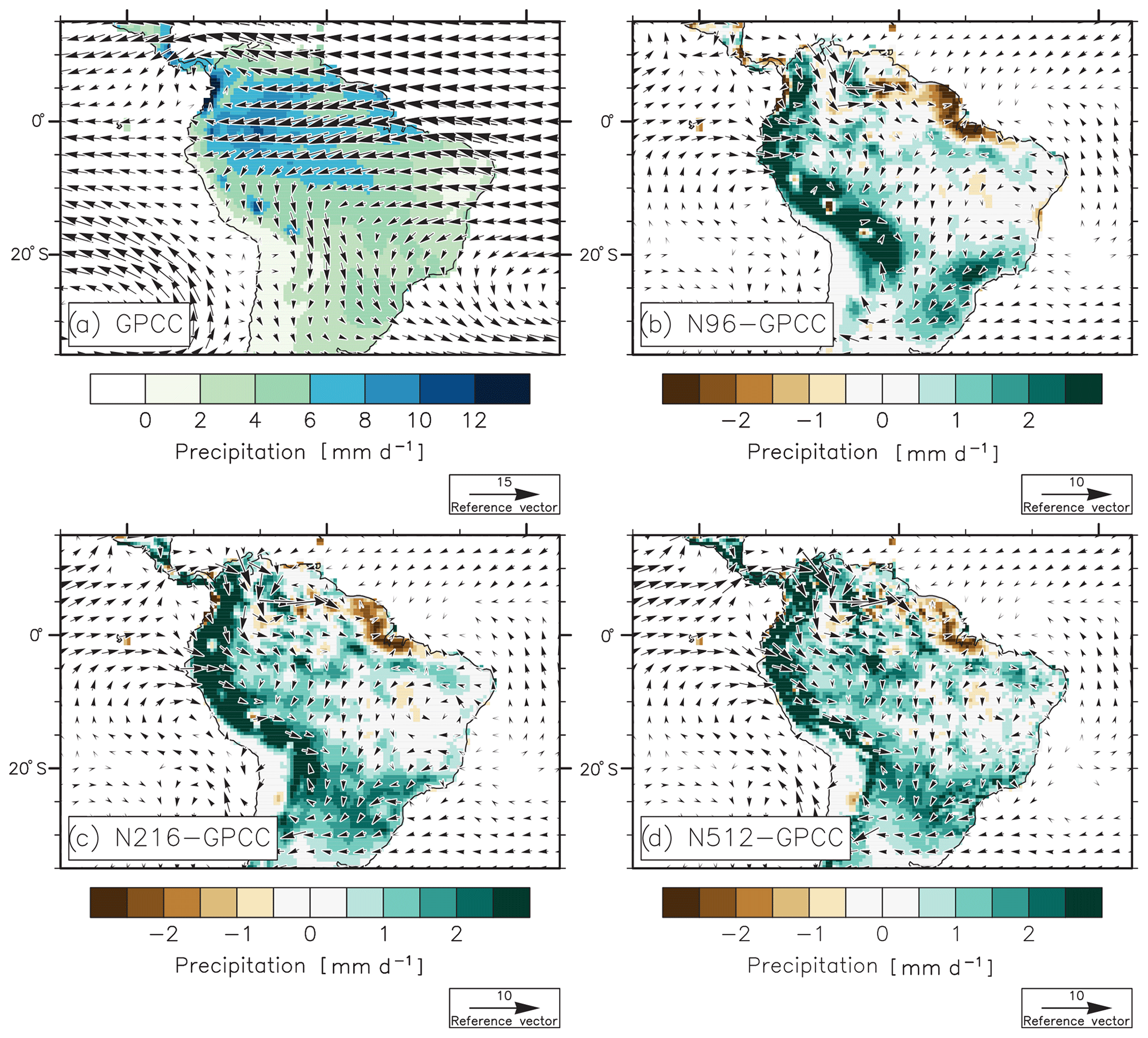
Figure 1(a) Observed mean annual precipitation (GPCC; mm d−1; colours) and 850 hPa wind (NCEP; m s−1; vectors), averaged over the period 1950–2014. Bias in precipitation and 850 hPa wind in (b) N96 (i.e. N96–GPCC), (c) N216 (i.e. N216–GPCC), and (d) N512 (i.e. N512–GPCC). In panels (a), (b), and (c) biases in precipitation are shown when statistically significant in all of the three members according to a Student's t test and a 95 % confidence level.
HadGEM3 has clear deficiencies in simulating precipitation, particularly over high orography. N96 has a wet bias over southern Brazil and over the Andes, from 30∘ S to the Equator, and a dry bias over northeast Brazil (Fig. 1b). Biases are strong: up to 3 mm d−1 over the Andes. The dry bias over northeast Brazil is associated with anomalously weak easterlies (Fig. 1b). An anomalously strong cyclonic circulation, located over Peru, weakens the easterlies between 10∘ S and the Equator, decreasing moisture flux divergence over the western Amazon Basin associated with a wet bias there (Fig. 1b). There is an anomalously strong anticyclonic circulation over southeast Brazil, which is associated with stronger easterlies from the South Atlantic Ocean to southern Brazil and a wet bias (Fig. 1b).
N216 and N512 also show wet biases over the Andes and southeastern Brazil and dry biases over northeast Brazil (Fig. 1c and d). Biases in low-level winds are also very similar in N96, N216, and N512. We highlight the impacts of each step change in resolution by displaying differences between all pairs of simulations. The total impact of shifting from N96 to N512 is given by N512–N96; intermediate steps are illustrated by N216–N96 and N512–N216. This helps to define the minimum resolution required to extract substantial simulation improvements from the available sets of simulations. The strongest impact of increasing resolution is over the Andes, where N512–N96 reaches up to 2 mm d−1 (Fig. 2c). Significant differences are also obtained over the Amazon Basin, northeast Brazil, and northwest Argentina (Fig. 2a–c). Over the Amazon Basin and the Andes, changes in precipitation in N512–N96 are due to both N216–N96 and N512–N216 (Fig. 2a and Fig. 2b). In addition, differences consist of reduced precipitation (Fig. 2a, b, c), and thus in reduced wet biases, over the Andes (Fig. 1bcd; see the stippling). Therefore, it is worth increasing horizontal resolution to N512 for simulating precipitation over the Andes.

Figure 2Ensemble-mean (a) N216–N96, (b) N512–N216, and (c) N512–N96 differences in mean annual precipitation (mm d−1). (d, e, f) Same as (a), (b), and (c) but for evaporation (mm d−1). (g, h, i) Same as (a), (b), and (c) but for the moisture flux convergence (P−E; mm d−1; colours) and the 850 hPa wind (m s−1; vectors). For precipitation (i.e. a–c) stippling indicates that the mean bias is reduced at the higher rather than at the lower horizontal resolution. Differences are shown when significantly different to zero according to a Student's t test and a 95 % confidence level.
Over northern Argentina, significant changes are only due to N216–N96 (Fig. 2a), while there are no significant changes in N512–N216 (Fig. 2b). Over the Amazon Basin, significant changes are found in both N216–N96 and N512–N216. Over the Amazon Basin and northern Argentina, increasing resolution increases precipitation, which strengthens the N96 wet bias. Over northeastern Brazil, the significant increase in precipitation with resolution reduces the N96 dry bias. However, the improvement is primarily found in N216–N96; resolutions higher than N216 do not appear to be useful. Over the ocean, increased resolution is associated with strong changes in precipitation; i.e. precipitation increases over the eastern Pacific Ocean and decreases over the tropical Atlantic Ocean (especially just offshore of most coastal regions) (Fig. 2), but most of the effect comes from moving from N96 to N216.
Changes in evaporation with resolution are significant over the eastern Pacific Ocean and over the southwest Atlantic Ocean along the coast of South America (Fig. 2d–f). However, increasing resolution leads to only moderate changes in evaporation over land. Unlike evaporation, differences in moisture flux convergence (i.e. precipitation minus evaporation) are strong over both land and ocean (Fig. 2g–i). Therefore, the sensitivity of Amazon Basin and Andes precipitation to resolution is mostly due to sensitivity in moisture transport rather than in local moisture recycling (i.e. conversion of local evaporation into precipitation). This is consistent with Vannière et al. (2019), who showed that ocean-to-land moisture advection increases with resolution. We show small changes in specific humidity and surface air temperature over land (Figs. S1 and S2 in the Supplement). This suggests that changes in precipitation with resolution are due to dynamic changes rather than thermodynamic changes. Increased resolution is associated with an eastward shift, toward the coast, of the southeast Pacific anticyclonic circulation (Fig. 2g–i) in the southern Pacific coastal region. The wind speed then strengthens and increases evaporation (Fig. 2d–f) and decreases moisture convergence (Fig. 2g–i). Over land, changes in wind speed are particularly strong over the mountains.
3.2 Seasonal means
We next examine the influence of resolution on seasonal rainfall, motivated by the strong seasonal cycle of South American rainfall (i.e. heavy rainfall over northern South America in July–September, while the Amazon Basin is wetter in DJF than in JAS). Over northeast Brazil, the resolution sensitivity is strongest in DJF and MAM, mainly due N216–N96 (Fig. 3a, c, d, and f), while the N512–N216 differences are moderate (Fig. 3b and e). Differences are also strong over the Amazon Basin, in DJF and SON, where increased resolution increases mean precipitation (Fig. 3c and l). Changes in Amazon Basin precipitation are contributed by both N216–N96 (Fig. 3a and j) and N512–N216 (Fig. 3b and k).
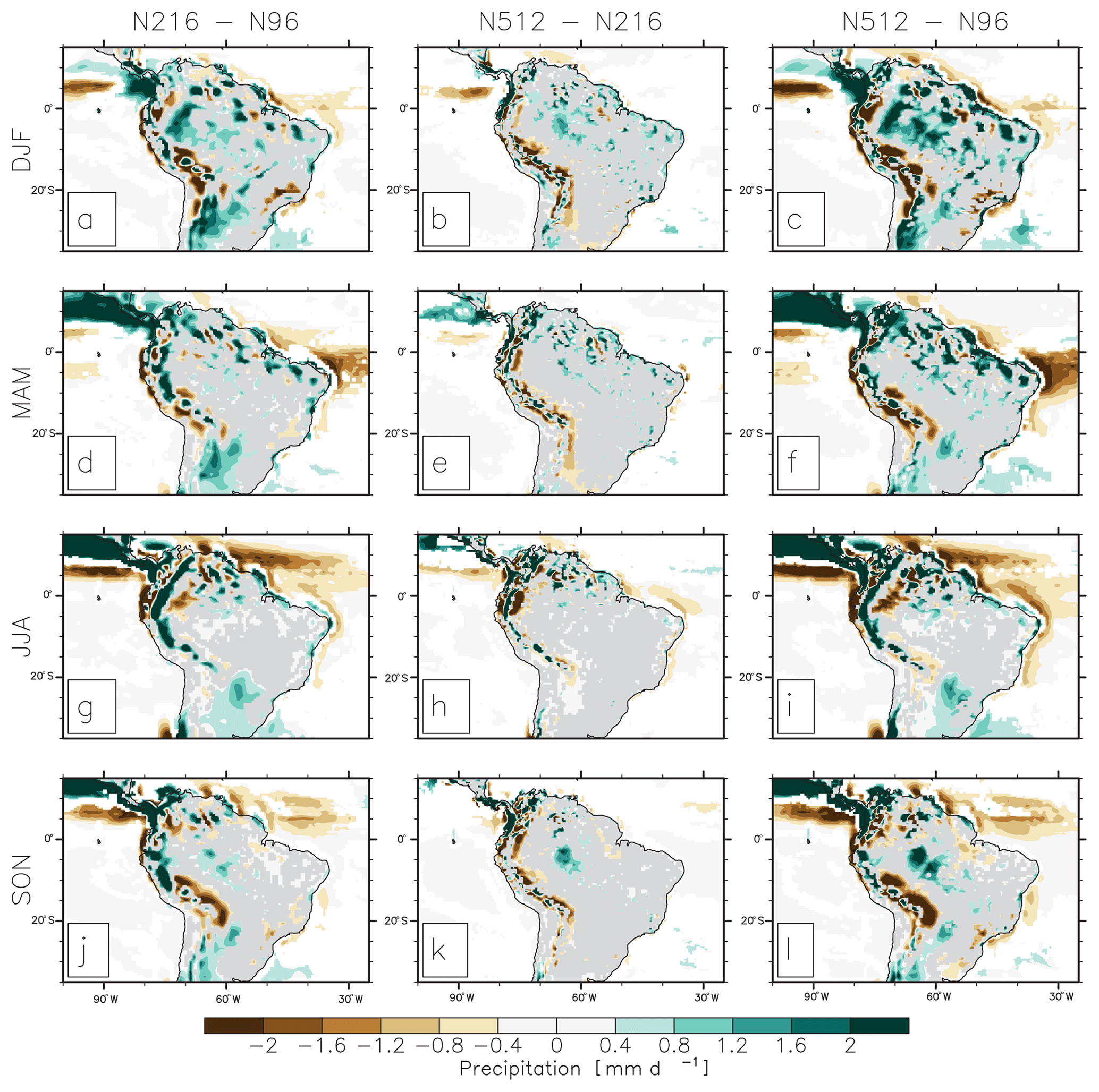
Figure 3Ensemble-mean N216–N96 difference in (a) DJF, (d), MAM, (g) JJA, and (j) SON precipitation (mm d−1). (b, e, h, k) As in (a), (d), (g), and (j) but for N512–N216. (c, f, i, l) As in (a), (d), (g), and (j) but for N512–N96. Differences are shown when statistically different to zero according to a Student's t test and a 95 % confidence level.
Over southwestern-Brazil–northern-Argentina, increasing resolution increases precipitation in all seasons, which increases the wet bias. These changes are only due to N216–N96 (Fig. 3). Strong differences are also obtained over the tropical Pacific and Atlantic Ocean, from March to November (Fig. 3d, g, and j), mainly due to N216–N96. N512–N216 does not strongly affect oceanic precipitation (Fig. 3e, h, and k).
Improvements are shown over northeast Brazil in DJF and MAM. There is little sensitivity to resolution elsewhere in South America. Over the Amazon, changes are stronger in austral summer (i.e. DJF) during the monsoon, but biases are higher at high resolution.
We have shown a limited effect of resolution on mean precipitation. However, climate variability could be more sensitive to resolution because resolution may affect how the model simulates precipitation distribution, local and large-scale atmospheric dynamics, land–atmosphere coupling, and mesoscale systems. Assessing climate variability provides useful information on the ability of climate models to simulate the climate system.
The pattern in annual precipitation variance follows the pattern in annual mean precipitation, i.e. higher along the Equator than over the surrounding regions (Fig. 4a). At all resolutions, HadGEM3 overestimates precipitation variability over southeast Brazil and underestimates precipitation variability between 15∘ S and the Equator (Fig. 4b–d). HadGEM3 overestimates both mean precipitation and precipitation variability over parts of the Andes and southeast-Brazil–northern-Argentina (Figs. 1b–d and 4b–d). HadGEM3 has a mean wet bias but underestimates the precipitation variability over the Amazon Basin, although increasing resolution reduces the variability bias (Fig. 4e–g). Over southeast Brazil, increasing resolution slightly reduces the overestimation of precipitation variance (Fig. 4e–g). There are no changes in precipitation variance over northeast Brazil in N512–N96 (Fig. 4e, f, and g).

Figure 4(a) Observed annual-mean precipitation variance (GPCC; mm2 d−2), as computed over the period 1982–2014. A linear trend is removed. Bias in annual-mean precipitation variance in (b) N96 (i.e. N96–GPCC), (c) N216 (i.e. N216–GPCC), and (d) N512 (i.e. N512–GPCC). (e) N216–N96, (f) N512–N216, and (g) N512–N96 differences in annual-mean precipitation variance. In (b), (c), and (d), biases are shown when all three members produce a bias that is significant according to an f test and a 95 % confidence level. In (e), (f), and (g), stippling indicates that the bias is improved at the higher rather than at the lower resolution.
Precipitation variance also increases with resolution for individual seasons (not shown). Because both Pacific and Atlantic SSTs affect seasonal-to-interannual South American precipitation variability, we hypothesised that changes in variance were associated with a change in the strength of the teleconnection between ENSO and South American precipitation and between the South Atlantic SSTs and South American precipitation. However, this hypothesis was not supported by the following evidence: the impact of ENSO on South America is assessed through regressing the El Niño 3.4 index (5∘ S–5∘ N, 170–120∘ W) onto precipitation for each grid point, focusing on the seasonal anomalies (Fig. S3). We found that increasing horizontal resolution does not systematically alter the influence of ENSO on Brazilian precipitation. These analyses were repeated, focusing on tropical Atlantic gradients in SST, yielding a similar conclusion to the one for ENSO; i.e. increasing the horizontal resolution does not change impacts of the SST on precipitation over land (not shown).
5.1 Daily variability
Daily precipitation variance is more sensitive to resolution that monthly or annual variance. Over the Amazon Basin, differences between the simulations are stronger in austral summer than in other seasons (Fig. S4). Moreover, precipitation variability is strongly tied to the South American summer monsoon, which mainly occurs in DJF. Therefore, we focus further analysis on daily variance and on DJF.
In DJF, N96 underestimates daily precipitation variance (Fig. 5a). N216 and N512 outperform N96, with a reduced underestimation of precipitation variance over the Amazon Basin (Fig. 5b and c). The increase in variance is due to shifts from N96 to N216 and N216 to N512 (Fig. 5d and e). The difference in P−E variance is high and close to the difference in P variance (Fig. 5g, h, and i). Therefore, changes in precipitation variance are mostly associated with changes in the variance of moisture flux convergence.

Figure 5(a–c) Bias in daily precipitation variance (mm2 d−2) for (a) N96 (i.e. N96–GPCC), (b) N216 (i.e. N216–GPCC), and (b) N512 (i.e. N512–GPCC) simulations over the DJF period. Seasonal cycle and linear trend are removed prior to computing variance. Differences in daily precipitation variance (mm2 d−2) for (d) N216–N96, (e) N512–N216, and (f) N512–N96. (g, h, i) As in (d), (e), and (f) but for P−E (precipitation minus evaporation) variance.
Biases in DJF daily precipitation variance have also been assessed using CMORPH over 1998–2014. The same conclusions are drawn: N96 underestimates variance and N512 overestimates variance (Fig. S4). However, the N96 biases are much reduced when compared to CMORPH instead of GPCC, such that N96 outperforms N216 and N512 (Figs. S4 and S5). In addition, the northern Brazil circulation is dominated by easterlies (Fig. 1a), whose variability is reinforced by increasing the horizontal resolution (Fig. S6). Over southern Brazil, the circulation is dominated by northerlies; increasing resolution increases meridional wind variance (Fig. S7). Therefore, we suggest that the change in precipitation variance is associated with changes in atmospheric dynamics. Positive feedback exists since an increase in precipitation is associated with a strengthening of local vertical velocity, which strengthens the low-level wind. However, changes in wind variance exhibit a large-scale pattern that suggests changes that are not due solely to local precipitation increases. The variance of the meridional wind increases strongly over the eastern side of the Andes (Fig. S7), highlighting the importance of the orography in modulating the circulation and transporting moisture.
We analysed the variance of the zonal and meridional components of the moisture flux and found the same patterns as for the low-level wind (not shown), suggesting that changes are mostly attributed to dynamic changes rather than thermodynamic changes.
5.2 Effects of the Madden–Julian oscillation
The MJO strongly affects sub-seasonal precipitation variability over Brazil (Grimm, 2019; Grimm and Silva Dias, 1995; Grimm and Tedeschi, 2009; Lewis et al., 2011; Marengo et al., 2008, 2011, 2013). Therefore, a change in the MJO teleconnection to South America may alter precipitation mean and variance.
Indices of the MJO have been computed using NCEP for observed wind and outgoing longwave radiation from NOAA Cooperative Institute for Research in Environmental Sciences dataset (Liebmann and Smith, 1996), following Wheeler and Hendon (2004), by computing empirical orthogonal functions on daily values of 850 and 200 hPa zonal winds and outgoing longwave radiation. Simulated MJO indices are performed by projecting model data onto the reanalysis empirical orthogonal functions (EOFs), after first removing the model annual mean and the first three harmonics of the model annual cycle. MJO indices were computed on data first interpolated on a 2.5∘ resolution. See Wheeler and Hendon (2004) for a longer description of the method. Time series have been deseasonalised and linearly detrended prior to computing impacts of MJO on precipitation mean and variance.
In observations (GPCC), the MJO strongly impacts tropical South American precipitation, leading to above-average precipitation during phases 1 and 8, while phases 3, 4, and 5 are associated with anomalously dry conditions (Fig. 6, top two rows), as shown in Grimm (2019). South of 20∘ S, phases 1, 7, and 8 are associated with anomalously dry conditions and phases 3, 4, and 5 with anomalously wet conditions (Fig. 6a, c–e, g, h). We select two areas, the Amazon Basin, where differences in precipitation variance between simulations are strong, and east Brazil, which is strongly impacted by the MJO. Note the boxes in Fig. 6a. Both areas experience above-average precipitation during MJO phases 1, 7, and 8 and below-average precipitation during phases 3, 4, and 5 (Fig. 6a–b). HadGEM3 reproduces the impact of MJO on east Brazil and Amazon Basin precipitation in sign and magnitude (Fig. 6i–j). There are no clear differences between N96, N216, and N512 simulations, and an impact of the horizontal resolution does not emerge.
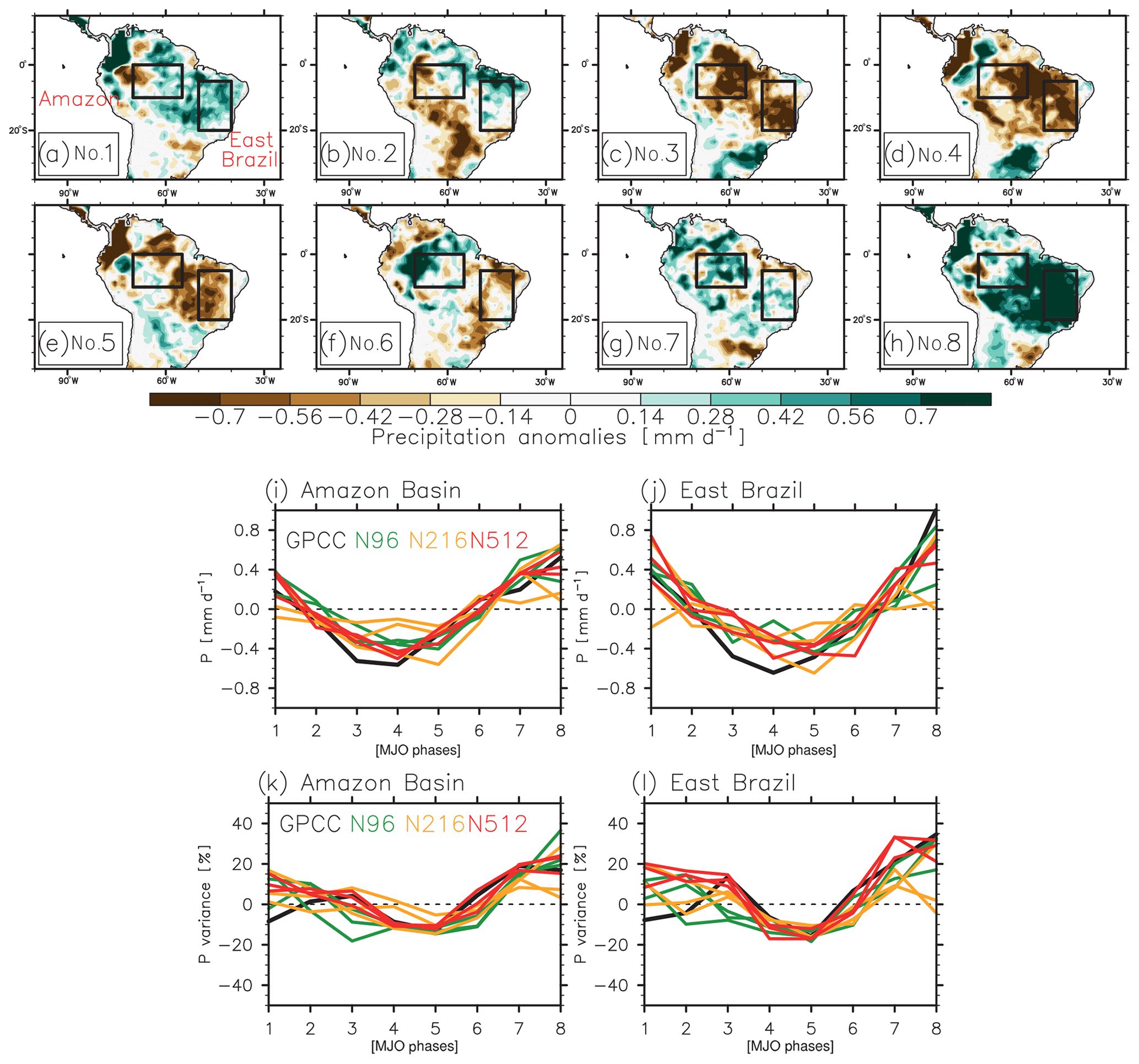
Figure 6Observed impacts of Madden–Julian oscillation phase (a) 1, (b) 2, (c) 3, (d) 4, (e) 5, (f) 6, (g) 7, and (h) 8 on precipitation (GPCC and NCEP for the RMM index; mm d−1). Precipitation anomalies (mm d−1), associated with each phase of the Madden–Julian oscillation, relative to the period 1982–2014, and averaged over the (i) Amazon Basin and (j) East Brazil (see the box in a), for observation (black), N96 (green), N216 (orange), and N512 (red). (k, l) As in (i) and (j) but for precipitation variance, in percent (%) of the precipitation variance over the period 1982–2014.
We show strong impacts of resolution on precipitation variance in Sect. 5.1. Therefore, we address here how precipitation variance could be affected by resolution within each MJO phase. Results are given relative to the variance of the precipitation computed from the full original daily time series (with no selection of any specific MJO phases). Results for precipitation variance differ slightly from those for the mean precipitation, with for instance a decrease in the variance during phase 1 when mean precipitation is higher and stronger during phase 3 when mean precipitation is lower. This difference could also arise from local differences that could strongly impact the area average. HadGEM3 simulates the impact of the MJO on the precipitation variance well, with above-average variance during phases 7 and 8 and below-average variance during phases 4 and 5. Unlike the observation, HadGEM3 simulates an increase in the variance of the precipitation during phase 1 of the MJO. N216 and N512 simulations perform better than N96 for phase 3 of the MJO, since N96 simulates reduced precipitation variance, while the variance is anomalously high in observations and in the N512 and N216 simulations. However, there is no clear sensitivity of MJO-related precipitation variance to horizontal resolution.
5.3 Land–atmosphere feedback
Soil moisture memory contributes to atmospheric variability and could potentially affect the development of the South American Monsoon System. Land–atmosphere coupling is particularly strong over South America (Koster et al., 2004; Sörensson and Menéndez, 2011). In this section we assess the sensitivity of land–atmosphere feedbacks to resolution, using ERA-interim as verifying “observations”. The coupling strength metric is defined as the correlation between two variables, weighted by the standard deviation of the reference variable (see Sect. 2.4).
Over the Amazon Basin, there is a positive relationship between observed precipitation and observed soil moisture (Fig. 7a), such that an increase in precipitation is associated with anomalously high soil moisture, with soil moisture being coincident with changes in precipitation (Fig. 7e). Over the Amazon Basin and in all HadGEM3 resolutions, the bias in the precipitation–soil-moisture coupling strength is small (Fig. 7b–d) and an increase in the resolution does not change precipitation–soil-moisture coupling strength (Fig. 7i–k, l–n), probably because, over the Amazon, the soil is saturated, such that increases in precipitation variability do not impact soil moisture variability. Soil moisture and evaporation are negatively correlated in observations over the Amazon Basin (Fig. 8a), such that increased evaporation decreases soil moisture. Over the Amazon Basin, there is no strong lead–lag relationship between soil moisture and evaporation in observations (Fig. 8e) or in HadGEM3 (Fig. 8f–h). The coupling strength is overestimated in N96 (Fig. 8b) but an increase in resolution reduces this overestimation (Fig. 8c–d and f–g). Over the Amazon Basin, the moisture budget is energy-limited rather than moisture limited (Cook et al., 2014). Therefore, we also assessed the coupling strength between temperature and evaporation. An increase in temperature is associated with increased evaporation (Fig. S8) and thus decreased soil moisture, but, in HadGEM3, this coupling strength is not sensitive to resolution (Fig. S8). These results are consistent with our previous results, showing that local recycling plays a moderate role in explaining changes in precipitation variance, which is mainly associated with change in the moisture flux convergence variability (Fig. 6) rather than with a stronger land–atmosphere coupling (Fig. 8).
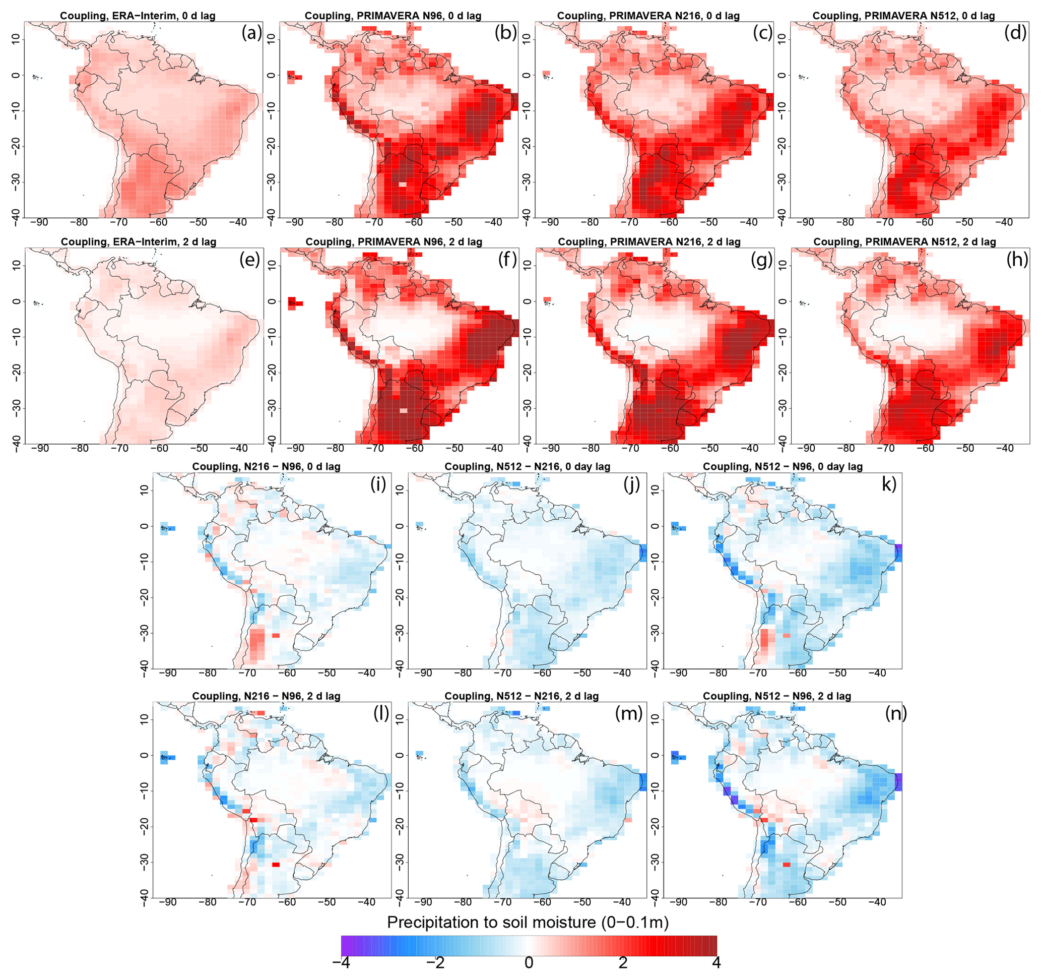
Figure 7(a) Observed (ERA-Interim) and (b) N96, (c) N216, and (d) N512 coupling strength (ra,bσb) between daily precipitation and soil moisture (in the top 0.1 m of soil) during the southern summer wet season (DJF), over the period 1979–2014. Two-dimensional time lag (i.e. the soil situation 2 d after precipitation) for (e) ERA-Interim, (f) N96, (g) N216, and (h) N512. (i) N216–N96, (j) N512–N216, and (k) N512–N96 coupling strength. (l, m, n) As for (i), (j), and (k) but with a 2 d time lag between precipitation and soil moisture.

Figure 8As in Fig. 7 but for the coupling strength between daily soil moisture (in the top 0.1 m of soil) and latent heat flux (LHF).
Outside of the Amazon Basin, the soil-moisture–precipitation relationship is positive in both observations (Fig. 7a) and HadGEM3 (Fig. 7b–d), with precipitation variability leading soil moisture variability (Fig. 7b and f–h). The increase in soil moisture increases evaporation over eastern Brazil (Fig. 8a). The soil-moisture–evaporation coupling strength is too high in all simulations over northeastern and eastern Brazil (Fig. 8b–d), with soil moisture driving evaporation because evaporation is moisture-limited over northeast Brazil, with changes in evaporation leading changes in temperature (Fig. S8). The strengths of both precipitation–soil-moisture and soil-moisture–evaporation couplings are overestimated in N96 (Figs. 7b and 8b) over eastern Brazil and southeastern South America. Increasing resolution reduces this overestimation (Figs. 7c, d, i–k; 8c, d, i–k).
5.4 Scales of precipitation
We use the ASoP diagnostics (see Sect. 2.4) to assess daily precipitation features over South America in HadGEM3 and verify them against CMORPH. We compute the fractional contribution to total CMORPH precipitation from four precipitation intensity bins, over South America, with a focus over two subregions, the Amazon Basin (AMZ) and southeast South America (SESA). We compare spatial and temporal scales of precipitation features across datasets for the two subregions. Results are given separately for light, moderate, and heavy rainfall events. We focus on the occurrence and duration of dry spells.
5.4.1 Light precipitation and dry spells
In CMORPH, light precipitation events (<10 mm d−1) contribute the most of all intensity categories to total precipitation over most of the Andes and northern and southern South America, the Pacific Ocean, and western Atlantic Ocean (Fig. 9a). N96 underestimates contributions from light precipitation events over the Andes and southeast Brazil but overestimates contributions from light precipitation over the Amazon Basin and northeastern Brazil (Fig. 9e). The results are consistent with Seth et al. (2004), who also show an overestimation of the percentage of light rain events over South America. This bias is reduced by increasing resolution to N216 and N512 (Figs. 9i–p; S9).
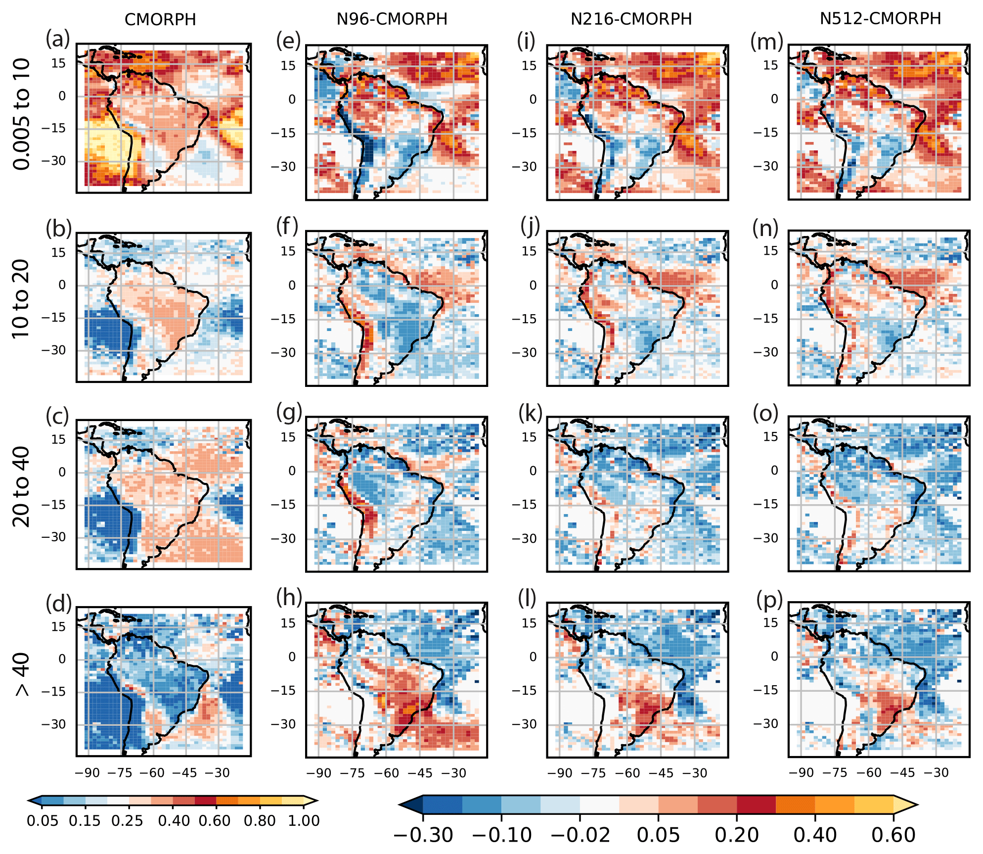
Figure 9Fractional contribution to the total precipitation from ranges of intensity bins shown in the labels above each panel for CMORPH (a–d) (the sum of each column is unity). Differences in the fractional contributions compared against CMORPH for N96 (e–f), N216 (i–l), and N512 (m–p) (all on the N96 common grid). The four ranges of intensity bins are (first row) 0.005 to 10 mm d−1, (second row) 10 to 20 mm d−1, (third row) 20 to 40 mm d−1, and (last row) >40 mm d−1.
Figure 10 shows frequencies of precipitation events, as classified by intensity and duration. Results are shown for two regions: AMZ, where variance is too weak, and SESA, where variance is too high. Over AMZ and SESA, near-zero precipitation (rainy events of 0.1–1 mm d−1) can last for more than 15 d, while events of 1–10 mm d−1 can last for up to 4 or 5 d (Fig. 10a and f). Over AMZ, N96 overestimates the frequency of events of 2 to 12 mm d−1 and underestimates the frequency of those of less than 1 mm d−1, compared to CMORPH (Fig. 10b). For SESA, N96 underestimates the frequency of precipitation events of less than 1 mm d−1 and lasting between 1 and 8 d; the model overestimates the frequency of near-zero rainy days, lasting more than 8 d (Fig. 10g). Intensity–duration biases improve with resolution over AMZ (Fig. 10c–d) and SESA (Fig. 10h–i). However, the biases worsen with resolution for near-zero precipitation lasting for any duration over AMZ and for intensities between 1 and 9 mm d−1 with a duration of 1–5 d over SESA.
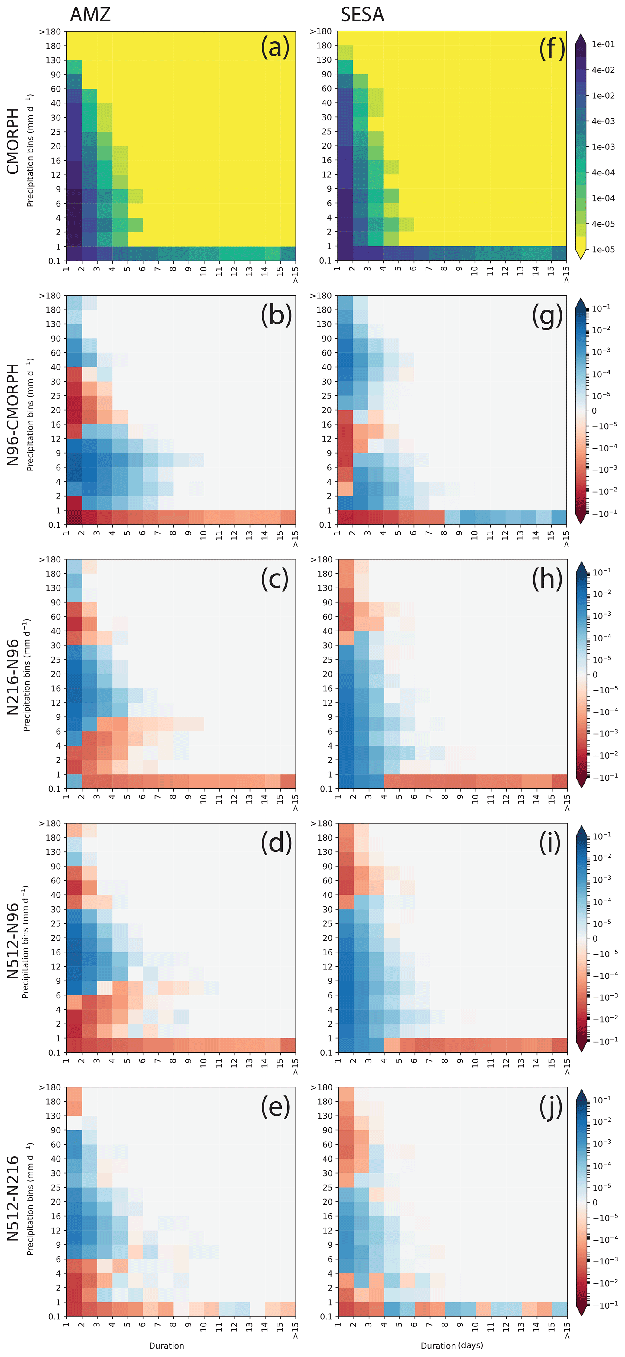
Figure 10Two-dimensional histograms of binned precipitation lasting for each duration bin, aggregated over all grid points and normalised by the number of spatial and temporal points in each dataset for (a) CMORPH for the AMZ region at N96 grid. Differences between the two-dimensional histograms for (b) N96 minus CMORPH, (c) N216 minus N96, (d) N512 minus N96, and (e) N512 minus N216 computed on the common N96 grid. Panels (f)–(j) are the same as (a)–(e) but for the SESA region.
In addition to events of less than 10 mm d−1, we assess simulated frequency and duration of dry spells, defined by events of less than 0.1 mm d−1. We create 2-D histograms for duration versus frequency of dry days over AMZ and SESA (Fig. 11). CMORPH shows more frequent short-duration dry spells as compared to HadGEM3 over AMZ at both native (Fig. 11a) and N96 (Fig. 11c) resolutions. Over SESA, CMORPH also generally shows more frequent dry spells for durations longer than 1 d (Fig. 11b, d). The sensitivity of dry-spell frequency to model resolution is generally smaller than the model bias. Once all datasets are interpolated to the common N96 resolution, N96 produces longer and more frequent dry spells than N216 and N512 and is closer to CMORPH.

Figure 11Histograms of dry days (with precipitation less than 0.1 mm d−1) lasting for each duration bin, aggregated over all grid points and normalised by the number of spatial and temporal points in each dataset: (a) Amazon and (b) SESA at native resolution for all datasets. Panels (c)–(d) are the same as (a)–(b) but for datasets on the common N96 grid.
5.4.2 Moderate precipitation
Over most other parts of South America (i.e. the Amazon and central and eastern Brazil), most of the total precipitation is contributed by light to moderate events (10–40 mm d−1; Fig. 9a–c). Compared to CMORPH, N96 overestimates the contribution from moderate events to total precipitation over the Andes and underestimates this contribution over South America outside of the Andes (Fig. 9f, g). Although the spatial pattern of biases is similar to N96, biases in contribution from moderate rainfall to total precipitation reduce when increasing resolution (Figs. 9f–j–n and g–k–o; S9).
Over AMZ and SESA, most precipitation comes from moderate events in both CMORPH and HadGEM3 (Fig. 10b–e). Over AMZ, CMORPH distribution peaks at ∼30 mm d−1 (Fig. 10b, d) when using the CMORPH native grid (Fig. 10b) and at ∼20 mm d−1 when using the N96 grid (Fig. 10d). At their native resolutions, N96, N216, and N512 have a primary peak at ∼9 mm d−1 and a secondary peak at ∼30 mm d−1 (Fig. 10b). On the N96 grid, the secondary peak is removed in N216 and N512. As the fractional contribution in HadGEM3 peaks at lower intensities for all three resolutions, HadGEM3 overestimates the contribution from intensities below ∼15 mm d−1 and underestimates contribution from intensities above 15 mm d−1 (Fig. 10b). When compared on their native grids, the model biases reduce with resolution over AMZ. However, once interpolated to N96, N512 has the largest bias in fractional contribution, around the peak intensity (i.e. at ∼10 mm d−1). Over AMZ, N96 underestimates the frequency of events of 12–40 mm d−1 (Figs. 10d and 12b). Increasing resolution reduces the biases for the frequency of events of 12–25 mm d−1 but leads to an underestimation of precipitation of 30 to 40 mm d−1 (Figs. 10b and 12c–e). Over SESA, distribution peaks at ∼20–30 mm d−1 (Fig. 12c and e). Over SESA, N96 underestimates (overestimates) the frequency of events of 2–20 mm d−1 (20–40 mm d−1) (Figs. 10g, 12e). These biases are reduced at N216 and N512 (Figs. 10h–j, 12e).
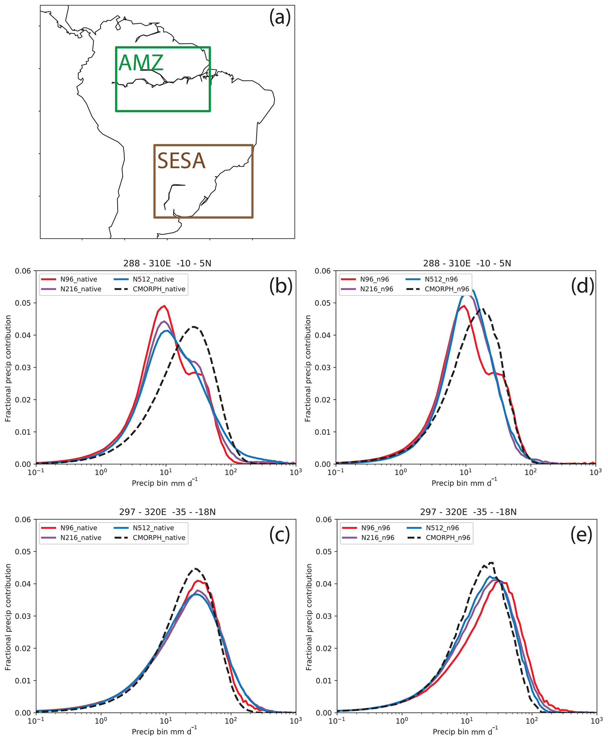
Figure 12(a) Subregions used in our study: (i) the Amazon region (AMZ; green box; 10∘ S–5∘ N, 72–50∘ W) and (ii) the southeast South America region (SESA; brown box; 35–18∘ S, 63–40∘ W). Histograms of the average precipitation contributions to the total precipitation from each precipitation bin for CMORPH and all simulations on their native grids for (b) AMZ and (c) SESA. Panels (d)–(e) are the same as (b)–(c) but at N96 grid.
5.4.3 Heavy precipitation
Parts of the Peruvian Andes, Uruguay, and northeastern Argentina receive most of their rainfall from heavy events (>40 mm d−1; Fig. 9d). N96 overestimates these contributions (>40 mm d−1) over central Brazil, the eastern Amazon, and southeastern Brazil (Fig. 9h). Like for the light and moderate events, increasing resolution reduces these biases (Figs. 9h–p and S9). This suggests that, at higher resolution, HadGEM3 performs better for the frequency of extreme events, such as those that lead to flooding. However, the improvements primarily come from the increase from N96 to N216, not from N216 to N512 (Fig. S9). In addition, N96 overestimates the frequency of events >40 mm d−1 over AMZ and SESA (Fig. 10b, g). Increasing resolution reduces these biases, again mostly due to increase from the N96 to N216 resolution, not from N216 to N512. For AMZ, N512 has a higher bias than N216 for events of 40–90 mm d−1.
5.4.4 Temporal and spatial scales
To compare spatial and temporal scales of precipitation features across datasets, we plot correlations as functions of distance (Fig. 13a–d) and time (Fig. 13e–h) (see Sect. 2.4). Over AMZ, N96 overestimates the spatial and temporal scales of precipitation events relative to CMORPH on their native grids (Fig. 13a and e). However, once CMORPH is interpolated to the N96 grid, the N96 simulation underestimates the spatial scale (and overestimates the temporal scale) of precipitation (Fig. 13b and f), highlighting that results strongly depend on the analysis grid. For SESA, N96 also underestimates the spatial scale and overestimates the temporal scale of precipitation (Fig. 13d–g–h). When considering native grids only, there are no clear differences between N96 and CMORPH for the spatial extent of precipitation events (Fig. 13c).
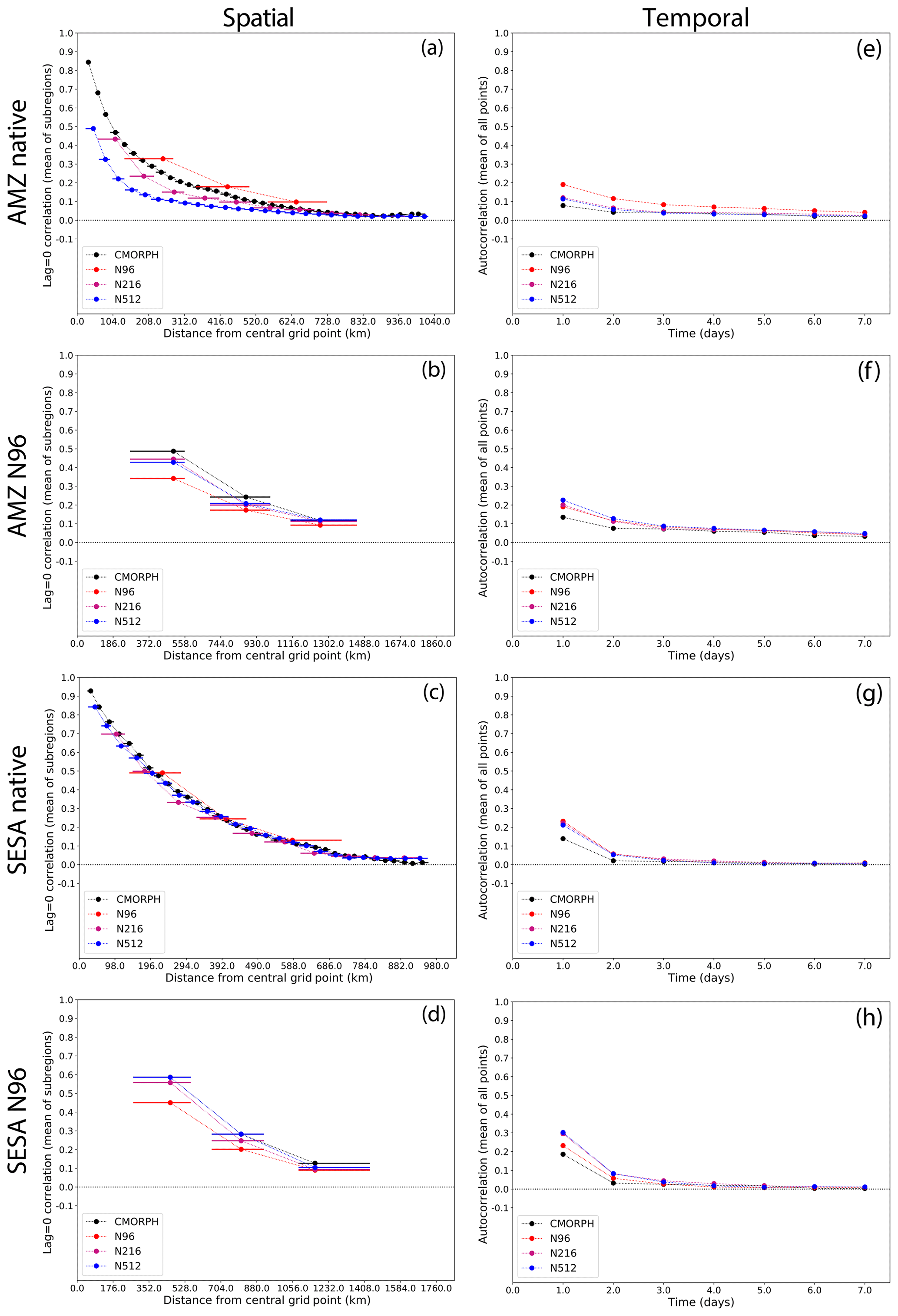
Figure 13(a) Metric of the spatial scale of daily precipitation (at native resolution), computed by dividing the analysis domain into 1500 km×1500 km subregions and calculating the mean lag-0 correlation between the central grid point and all grid points within each distance bin (which are 1x wide, starting from 0.51x) away from the central grid point and then averaging the correlations over all subregions in AMZ; (e) metric of the temporal scale of daily precipitation, computed as the autocorrelation at each point, averaged over all points AMZ. The horizontal lines in (a)–(d) show the range of distances spanned by each distance bin; the filled circle is placed at the median distance. For clarity, we omit the correlations for zero distance and zero lag, which are 1.0 by definition. Panels (b) and (f) are the same as (a) and (c) respectively for all datasets on the N96 grid; (c–d) and (g–h) are the same as (a–b) and (e–f) respectively but for SESA.
On native grids, N96 simulates events with larger spatial scales than N216 and N512 (Fig. 13a). However, this is mainly due to the coarse N96 grid. While all datasets are interpolated onto the N96 grid, N96 events are smaller than those in N216 and N512, which show similar scales and are closer to CMORPH (Fig. 13b). Over SESA, spatial scales are similar in all simulations, on their native grids (Fig. 13c). However, as for AMZ, at N96 resolution N512 and N216 are closer to CMORPH than to N96 (Fig. 13d). For both AMZ and SESA, therefore, the spatial features of daily precipitation events are better simulated at higher resolution.
At all resolutions, simulated precipitation features persist longer than in CMORPH (Fig. 13e–h). Over AMZ and SESA, biases are lowest in N96, which simulates events that are less persistent than in N216 and N512 (Fig. 13f, h). This bias increases at higher resolution. Therefore, increasing horizontal resolution does not improve biases in temporal scales of precipitation.
We assess the effects of increasing horizontal resolution on simulated South American precipitation. We use atmosphere-only simulations, performed with HadGEM3-GC3.1 (Williams et al., 2018) at three horizontal resolutions: N96 (∼130 km, ), N216 (∼60 km, ∘), and N512 (∼25 km, ). We assess, systematically, how the step change between each resolution effects simulated precipitation, focusing on precipitation mean and variance and on fine-scale processes, such as temporal and spatial scales, frequency of heavy and light precipitation events, and dry-spell durations.
We show that the atmosphere-only simulations have systematic biases in simulating annual mean and seasonal mean precipitation over South America. Northeast Brazil is anomalously dry, while southeast Brazil and the Andes are too wet. These biases are mostly due to atmospheric circulation biases: underestimated trade easterlies and a displaced anticyclonic circulation over southeast Brazil, both acting to modify moisture transport over South America. Increasing horizontal resolution affects the simulated precipitation. For instance, precipitation biases reduce over the Andes and over northeast Brazil. It is worth increasing the resolution to N512 (∼25 km) for simulating precipitation over the Andes Mountains. This is consistent with Vannière et al. (2019), who show that the added value of increasing horizontal resolution is greatest over orography. Over northeast Brazil, the largest improvement comes from increasing resolution to N216 (∼60 km); a further increase to N512 is only associated with moderate changes. Increasing resolution does not improve model biases over the Amazon Basin. These results are consistent with Roberts et al. (2018) for the Amazon Basin and northeast and south Brazil. In addition, improvements vary seasonally: changes are the strongest over northeast Brazil in DJF and MAM, when precipitation is also highest. Over the Andes, the results are similar in all seasons.
Biases in mean precipitation are collocated with biases in regional precipitation variance. For instance, northeast Brazil is too dry and HadGEM3-GC3.1 systematically underestimates precipitation variance, while southeast Brazil is too wet and HadGEM3-GC3.1 systematically overestimates precipitation variance. However, this does not hold for the Amazon Basin, which is too wet but where the precipitation variance is strongly underestimated. Precipitation variance is stronger at daily scales than at monthly scales; biases are strongest in DJF and over the Amazon Basin. Increasing resolution increases precipitation variance, hence reducing biases. The increase in precipitation variance is associated with an increase in moisture flux convergence variance over land and with changes in the variance of the low-level winds; local recycling of evaporation has a limited role. Relatedly, coupling strengths between evaporation, soil moisture, and precipitation are only weakly sensitive to resolution, except for some improvements in coupling strength over eastern and southeastern Brazil. We found only modest sensitivity to resolution for the teleconnections of the El Niño–Southern Oscillation and Madden–Julian oscillation to land precipitation. This suggests that changes in precipitation mean and variance are not due to changes in these teleconnections.
HadGEM3-GC3.1 has biases in its precipitation distribution. For instance, the model does not produce enough dry days over the Amazon Basin or moderate rain days (10–40 mm d−1), while simulating too many light events (<10 mm d−1) and heavy events (>40 mm d−1). Over southeast Brazil, the model simulates too few short dry spells and too many long ones. HadGEM3-GC3.1 simulates too few and too short events of 2 to 16 mm d−1, but simulates too many and too long events of more than 20 mm d−1. These metrics are important for understanding the ability of climate models to simulate high-impact events. Increasing resolution reduces these biases; N512 is therefore better at simulating precipitation distributions than N96. In addition, increasing the horizontal resolution increases the spatial scale of daily rain events, suggesting a better simulation of organised mesoscale systems. However, the persistence of precipitation events is better simulated at N96, showing no clear sensitivity to resolution. Other models also overestimate light events at the expense of heavy events over the Amazon and eastern Brazil and overestimate heavy events at the expense of lighter ones in southeast Brazil (Seth et al., 2004).
Over South America, precipitation results from the combination of the predominant role played by the Intertropical Convergence Zone and the South Atlantic Convergence Zone (Liebmann et al., 1999; Waliser et al., 1993). In addition, mesoscale systems such as squall lines may be responsible for a large fraction of Amazonian precipitation (Cohen et al., 1995). Our results show that increasing the horizontal resolution increases the spatial scale of rain events, i.e. of the mesoscale systems, over both Amazonia and southeast Brazil. Therefore, we speculate that increasing resolution could lead to more organised convective systems, which would be consistent with the increase in moisture flux convergence, as shown over South America at the highest resolution. This would be consistent with Vellinga et al. (2016), who showed that N512 resolution improved mesoscale systems over West Africa relative to N96 or N216. Conversely, the decrease in the persistence of such events (highest at the N96 resolution) could be associated with an increase in daily rainfall variability because of less persistent rainy events. Those are hypotheses that should be assessed in more detail in a specific study, potentially with models at sufficiently high resolution to disable convective parameterisations.
Although we hypothesised that increasing resolution might affect the ability of climate models to predict precipitation, Bombardi et al. (2018) have shown that an improvement in South American precipitation prediction due to an increase in resolution is not straightforward. In addition to resolution, further work should, therefore, be devoted to understanding the effects of physics on prediction system performance.
The mechanism for increases in precipitation variance with resolution are still unclear. The increase in precipitation variance is a global feature, not limited to South America (Fig. S10). Further work is needed to understand this behaviour better at a global scale. Moreover, we used Atmosphere Model Intercomparison Project (AMIP)-type simulations, and results could be different in coupled models, in which the ocean can interact with atmospheric variability, particularly when accounting for SST teleconnections.
Codes used to perform analysis and produce figures are publicly available at https://doi.org/10.5281/zenodo.3840095 (Monerie, 2020). For the analysis of the scales of precipitation (ASoP), codes are available at https://github.com/nick-klingaman/dubstep/tree/master/asop (Klingaman and Martin, 2020), https://github.com/nick-klingaman/dubstep/tree/master/asop_duration (Chevuturi, 2020), and https://doi.org/10.5281/zenodo.3997114 (Chevuturi et al., 2020).
The model data used in the analysis are available from the CMIP6 Earth System Grid Federation, for N96 (HadGEM3-GC31-LM; https://doi.org/10.22033/ESGF/CMIP6.1321; Roberts, 2017a), N216 (HadGEM3-GC31-MM; https://doi.org/10.22033/ESGF/CMIP6.1902; Roberts, 2017b), and N512 (HadGEM3-GC31-HM; https://doi.org/10.22033/ESGF/CMIP6.446; Roberts, 2017c). The list of persistent identifiers of the data we have used is available at https://doi.org/10.5281/zenodo.3840095 (Monerie, 2020).
The supplement related to this article is available online at: https://doi.org/10.5194/gmd-13-4749-2020-supplement.
AC, PAM, and PC performed the data analysis. PAM prepared the paper with contributions from all co-authors.
The authors declare that they have no conflict of interest.
Detailed calculations and code for the ASoP diagnostics are available at https://github.com/achevuturi/asop_duration (last access: January 2020). NOAA OLR data can be obtained from the website (https://www.esrl.noaa.gov/psd/data/gridded/data.interp_OLR.html, last access: January 2020). The authors thank Pier Luigi Vidale for his insightful and constructive comments. The authors thank the two anonymous reviewers for their constructive comments and suggestions.
This work was supported by the Newton Fund through the Met Office Climate Science for Service Partnership Brazil (CSSP Brazil). Nicholas P. Klingaman was funded by an Independent Research Fellowship from the Natural Environment Research Council (NE/L010976/1) and by the NERC/GCRF programme Atmospheric hazard in developing countries: risk assessment and early warnings (ACREW).
This paper was edited by Fabien Maussion and reviewed by two anonymous referees.
Bacmeister, J. T., Wehner, M. F., Neale, R. B., Gettelman, A., Hannay, C., Lauritzen, P. H., Caron, J. M., and Truesdale, J. E.: Exploratory High-Resolution Climate Simulations using the Community Atmosphere Model (CAM), J. Climate, 27, 3073–3099, https://doi.org/10.1175/JCLI-D-13-00387.1, 2013.
Bombardi, R. J. and Carvalho, L. M. V: IPCC global coupled model simulations of the South America monsoon system, Clim. Dynam., 33, 893, https://doi.org/10.1007/s00382-008-0488-1, 2008.
Bombardi, R. J., Trenary, L., Pegion, K., Cash, B., DelSole, T., and Kinter III, J. L.: Seasonal Predictability of Summer Rainfall over South America, J. Climate., 31, 8181–8195, https://doi.org/10.1175/JCLI-D-18-0191.1, 2018.
Chevuturi, A.: “asop_duration” – Wet-spell and dry-spell duration, GitHub, available at: https://github.com/nick-klingaman/dubstep/tree/master/asop_duration, last access: January 2020.
Chevuturi, A., Klingaman, N. P., and Martin, G.: nick-klingaman/dubstep: Initial DUBSTEP project release (Version v0.1), Zenodo, https://doi.org/10.5281/zenodo.3997114, 2020.
Coelho, C. A. S., de Oliveira, C. P., Ambrizzi, T., Reboita, M. S., Carpenedo, C. B., Campos, J. L. P. S., Tomaziello, A. C. N., Pampuch, L. A., Custódio, M. de S., Dutra, L. M. M., Da Rocha, R. P., and Rehbein, A.: The 2014 southeast Brazil austral summer drought: regional scale mechanisms and teleconnections, Clim. Dynam., 46, 3737–3752, https://doi.org/10.1007/s00382-015-2800-1, 2016.
Cohen, J. C. P., Silva Dias, M. A. F., and Nobre, C. A.: Environmental Conditions Associated with Amazonian Squall Lines: A Case Study, Mon. Weather Rev., 123, 3163–3174, https://doi.org/10.1175/1520-0493(1995)123<3163:ECAWAS>2.0.CO;2, 1995.
Collins, M., Minobe, S., Barreiro, M., Bordoni, S., Kaspi, Y., Kuwano-Yoshida, A., Keenlyside, N., Manzini, E., O'Reilly, C. H., Sutton, R., Xie, S.-P. and Zolina, O.: Challenges and opportunities for improved understanding of regional climate dynamics, Nat. Clim. Chang., 8, 101–108, https://doi.org/10.1038/s41558-017-0059-8, 2018.
Cook, B. I., Smerdon, J. E., Seager, R., and Coats, S.: Global warming and 21st century drying, Clim. Dynam., 43, 2607–2627, https://doi.org/10.1007/s00382-014-2075-y, 2014.
Custódio, M. de S., Porfírio da Rocha, R. and Vidale, P. L.: Analysis of precipitation climatology simulated by high resolution coupled global models over the South America, Hydrol. Res. Lett., 6, 92–97, https://doi.org/10.3178/hrl.6.92, 2012.
Custodio, M. de S., da Rocha, R. P., Ambrizzi, T., Vidale, P. L., and Demory, M.-E.: Impact of increased horizontal resolution in coupled and atmosphere-only models of the HadGEM1 family upon the climate patterns of South America, Clim. Dynam., 48, 3341–3364, https://doi.org/10.1007/s00382-016-3271-8, 2017.
Dai, A.: Precipitation Characteristics in Eighteen Coupled Climate Models, J. Climate, 19, 4605–4630, https://doi.org/10.1175/JCLI3884.1, 2006.
Dee, D. P., Uppala, S. M., Simmons, A. J., Berrisford, P., Poli, P., Kobayashi, S., Andrae, U., Balmaseda, M. A., Balsamo, G., Bauer, P., Bechtold, P., Beljaars, A. C. M., van de Berg, L., Bidlot, J., Bormann, N., Delsol, C., Dragani, R., Fuentes, M., Geer, A. J., Haimberger, L., Healy, S. B., Hersbach, H., Hólm, E. V, Isaksen, L., Kållberg, P., Köhler, M., Matricardi, M., McNally, A. P., Monge-Sanz, B. M., Morcrette, J.-J., Park, B.-K., Peubey, C., de Rosnay, P., Tavolato, C., Thépaut, J.-N., and Vitart, F.: The ERA-Interim reanalysis: configuration and performance of the data assimilation system, Q. J. Roy. Meteor. Soc., 137, 553–597, https://doi.org/10.1002/qj.828, 2011.
DelSole, T. and Shukla, J.: Model Fidelity versus Skill in Seasonal Forecasting, J. Climate, 23, 4794–4806, https://doi.org/10.1175/2010JCLI3164.1, 2010.
Delworth, T. L., Rosati, A., Anderson, W., Adcroft, A. J., Balaji, V., Benson, R., Dixon, K., Griffies, S. M., Lee, H.-C., Pacanowski, R. C., Vecchi, G. A., Wittenberg, A. T., Zeng, F., and Zhang, R.: Simulated Climate and Climate Change in the GFDL CM2.5 High-Resolution Coupled Climate Model, J. Climate, 25, 2755–2781, https://doi.org/10.1175/JCLI-D-11-00316.1, 2011.
Demory, M.-E., Vidale, P. L., Roberts, M. J., Berrisford, P., Strachan, J., Schiemann, R., and Mizielinski, M. S.: The role of horizontal resolution in simulating drivers of the global hydrological cycle, Clim. Dynam., 42, 2201–2225, https://doi.org/10.1007/s00382-013-1924-4, 2014.
De Sales, F. and Xue, Y.: Assessing the dynamic-downscaling ability over South America using the intensity-scale verification technique, Int. J. Climatol., 31, 1205–1221, https://doi.org/10.1002/joc.2139, 2011.
Doblas-Reyes, F. J., Andreu-Burillo, I., Chikamoto, Y., García-Serrano, J., Guemas, V., Kimoto, M., Mochizuki, T., Rodrigues, L. R. L., and van Oldenborgh, G. J.: Initialized near-term regional climate change prediction, Nat. Commun., 4, 1715, https://doi.org/10.1038/ncomms2704, 2013.
Eyring, V., Bony, S., Meehl, G. A., Senior, C. A., Stevens, B., Stouffer, R. J., and Taylor, K. E.: Overview of the Coupled Model Intercomparison Project Phase 6 (CMIP6) experimental design and organization, Geosci. Model Dev., 9, 1937–1958, https://doi.org/10.5194/gmd-9-1937-2016, 2016.
Falco, M., Carril, A. F., Menéndez, C. G., Zaninelli, P. G., and Li, L. Z. X.: Assessment of CORDEX simulations over South America: added value on seasonal climatology and resolution considerations, Clim. Dynam., 52, 4771–4786, https://doi.org/10.1007/s00382-018-4412-z, 2019.
Gent, P. R., Yeager, S. G., Neale, R. B., Levis, S., and Bailey, D. A.: Improvements in a half degree atmosphere/land version of the CCSM, Clim. Dynam., 34, 819–833, https://doi.org/10.1007/s00382-009-0614-8, 2010.
Grimm, A. M.: Madden–Julian Oscillation impacts on South American summer monsoon season: precipitation anomalies, extreme events, teleconnections, and role in the MJO cycle, Clim. Dynam., 53, 907–932, https://doi.org/10.1007/s00382-019-04622-6, 2019.
Grimm, A. M. and Silva Dias, P. L.: Analysis of Tropical–Extratropical Interactions with Influence Functions of a Barotropic Model, J. Atmos. Sci., 52, 3538–3555, https://doi.org/10.1175/1520-0469(1995)052<3538:AOTIWI>2.0.CO;2, 1995.
Grimm, A. M. and Tedeschi, R. G.: ENSO and Extreme Rainfall Events in South America, J. Climate, 22, 1589–1609, https://doi.org/10.1175/2008JCLI2429.1, 2009.
Haarsma, R. J., Roberts, M. J., Vidale, P. L., Senior, C. A., Bellucci, A., Bao, Q., Chang, P., Corti, S., Fučkar, N. S., Guemas, V., von Hardenberg, J., Hazeleger, W., Kodama, C., Koenigk, T., Leung, L. R., Lu, J., Luo, J.-J., Mao, J., Mizielinski, M. S., Mizuta, R., Nobre, P., Satoh, M., Scoccimarro, E., Semmler, T., Small, J., and von Storch, J.-S.: High Resolution Model Intercomparison Project (HighResMIP v1.0) for CMIP6, Geosci. Model Dev., 9, 4185–4208, https://doi.org/10.5194/gmd-9-4185-2016, 2016.
Jia, L., Yang, X., Vecchi, G. A., Gudgel, R. G., Delworth, T. L., Rosati, A., Stern, W. F., Wittenberg, A. T., Krishnamurthy, L., Zhang, S., Msadek, R., Kapnick, S., Underwood, S., Zeng, F., Anderson, W. G., Balaji, V., and Dixon, K.: Improved Seasonal Prediction of Temperature and Precipitation over Land in a High-Resolution GFDL Climate Model, J. Climate, 28, 2044–2062, https://doi.org/10.1175/JCLI-D-14-00112.1, 2014.
Joyce, R. J., Janowiak, J. E., Arkin, P. A., and Xie, P.: CMORPH: A Method that Produces Global Precipitation Estimates from Passive Microwave and Infrared Data at High Spatial and Temporal Resolution, J. Hydrometeorol., 5, 487–503, https://doi.org/10.1175/1525-7541(2004)005<0487:CAMTPG>2.0.CO;2, 2004.
Jung, T., Miller, M. J., Palmer, T. N., Towers, P., Wedi, N., Achuthavarier, D., Adams, J. M., Altshuler, E. L., Cash, B. A., Kinter, J. L., Marx, L., Stan, C., and Hodges, K. I.: High-Resolution Global Climate Simulations with the ECMWF Model in Project Athena: Experimental Design, Model Climate, and Seasonal Forecast Skill, J. Climate, 25, 3155–3172, https://doi.org/10.1175/JCLI-D-11-00265.1, 2011.
Kanamitsu, M., Ebisuzaki, W., Woollen, J., Yang, S.-K., Hnilo, J. J., Fiorino, M., Potter, G. L., Kanamitsu, M., Ebisuzaki, W., Woollen, J., Yang, S.-K., Hnilo, J. J., Fiorino, M., and Potter, G. L.: NCEP–DOE AMIP-II Reanalysis (R-2), B. Am. Meteorol. Soc., 83, 1631–1643, https://doi.org/10.1175/BAMS-83-11-1631, 2002.
Kirtman, B. P., Bitz, C., Bryan, F., Collins, W., Dennis, J., Hearn, N., Kinter, J. L., Loft, R., Rousset, C., Siqueira, L., Stan, C., Tomas, R., and Vertenstein, M.: Impact of ocean model resolution on CCSM climate simulations, Clim. Dynam., 39, 1303–1328, https://doi.org/10.1007/s00382-012-1500-3, 2012.
Klingaman, N. P. and and Martin, G.: title: “asop” – Analysis of Scales of Precipitation, available at: https://github.com/nick-klingaman/dubstep/tree/master/asop, last access: March 2020.
Klingaman, N. P., Martin, G. M., and Moise, A.: ASoP (v1.0): a set of methods for analyzing scales of precipitation in general circulation models, Geosci. Model Dev., 10, 57–83, https://doi.org/10.5194/gmd-10-57-2017, 2017.
Knight, J. R., Folland, C. K., and Scaife, A. A.: Climate impacts of the Atlantic Multidecadal Oscillation, Geophys. Res. Lett., 33, L17706, https://doi.org/10.1029/2006GL026242, 2006.
Koster, R. D., Dirmeyer, P. A., Guo, Z., Bonan, G., Chan, E., Cox, P., Gordon, C. T., Kanae, S., Kowalczyk, E., Lawrence, D., Liu, P., Lu, C.-H., Malyshev, S., McAvaney, B., Mitchell, K., Mocko, D., Oki, T., Oleson, K., Pitman, A., Sud, Y. C., Taylor, C. M., Verseghy, D., Vasic, R., Xue, Y., and Yamada, T.: Regions of Strong Coupling Between Soil Moisture and Precipitation, Science 305, 1138–1140, https://doi.org/10.1126/science.1100217, 2004.
Koutroulis, A. G., Grillakis, M. G., Tsanis, I. K., and Papadimitriou, L.: Evaluation of precipitation and temperature simulation performance of the CMIP3 and CMIP5 historical experiments, Clim. Dynam., 47, 1881–1898, https://doi.org/10.1007/s00382-015-2938-x, 2016.
Lewis, S. L., Brando, P. M., Phillips, O. L., van der Heijden, G. M. F., and Nepstad, D.: The 2010 Amazon Drought, Science, 331, p. 554, https://doi.org/10.1126/science.1200807, 2011.
Liebmann, B. and Smith, C. A.: Description of a Complete (Interpolated) Outgoing Longwave Radiation Dataset, B. Am. Meteorol. Soc., 77, 1275–1277, 1996.
Liebmann, B., Kiladis, G. N., Marengo, J., Ambrizzi, T., and Glick, J. D.: Submonthly Convective Variability over South America and the South Atlantic Convergence Zone, J. Climate, 12, 1877–1891, https://doi.org/10.1175/1520-0442(1999)012<1877:SCVOSA>2.0.CO;2, 1999.
Liu, W. T. and Juárez, R. I. N.: ENSO drought onset prediction in northeast Brazil using NDVI, Int. J. Remote Sens., 22, 3483–3501, https://doi.org/10.1080/01431160010006430, 2001.
Marengo, J. A., Nobre, C. A., Tomasella, J., Oyama, M. D., Sampaio de Oliveira, G., de Oliveira, R., Camargo, H., Alves, L. M., and Brown, I. F.: The Drought of Amazonia in 2005, J. Climate, 21, 495–516, https://doi.org/10.1175/2007JCLI1600.1, 2008.
Marengo, J. A., Tomasella, J., Alves, L. M., Soares, W. R., and Rodriguez, D. A.: The drought of 2010 in the context of historical droughts in the Amazon region, Geophys. Res. Lett., 38, L12703, https://doi.org/10.1029/2011GL047436, 2011.
Marengo, J. A., Alves, L. M., Soares, W. R., Rodriguez, D. A., Camargo, H., Riveros, M. P., and Pabló, A. D.: Two Contrasting Severe Seasonal Extremes in Tropical South America in 2012: Flood in Amazonia and Drought in Northeast Brazil, J. Climate, 26, 9137–9154, https://doi.org/10.1175/JCLI-D-12-00642.1, 2013.
Martin, G. M., Klingaman, N. P., and Moise, A. F.: Connecting spatial and temporal scales of tropical precipitation in observations and the MetUM-GA6, Geosci. Model Dev., 10, 105–126, https://doi.org/10.5194/gmd-10-105-2017, 2017.
McClean, J. L., Bader, D. C., Bryan, F. O., Maltrud, M. E., Dennis, J. M., Mirin, A. A., Jones, P. W., Kim, Y. Y., Ivanova, D. P., Vertenstein, M., Boyle, J. S., Jacob, R. L., Norton, N., Craig, A., and Worley, P. H.: A prototype two-decade fully-coupled fine-resolution CCSM simulation, Ocean Model., 39, 10–30, https://doi.org/10.1016/j.ocemod.2011.02.011, 2011.
Monerie, P.-A.: Scripts we used for “Role of atmospheric horizontal resolution in simulating tropical and subtropical South American precipitation in HadGEM3-GC31” [Data set], Zenodo, https://doi.org/10.5281/zenodo.3840095, 2020.
Power, S., Casey, T., Folland, C., Colman, A., and Mehta, V.: Inter-decadal modulation of the impact of ENSO on Australia, Clim. Dynam., 15, 319–324, https://doi.org/10.1007/s003820050284, 1999.
Rayner, N. A., Brohan, P., Parker, D. E., Folland, C. K., Kennedy, J. J., Vanicek, M., Ansell, T. J., and Tett, S. F. B.: Improved Analyses of Changes and Uncertainties in Sea Surface Temperature Measured In Situ since the Mid-Nineteenth Century: The HadSST2 Dataset, J. Climate, 19, 446–469, https://doi.org/10.1175/JCLI3637.1, 2006.
Roberts, M.: MOHC HadGEM3-GC31-LM model output prepared for CMIP6 HighResMIP. Version YYYYMMDD[1], Earth System Grid Federation, https://doi.org/10.22033/ESGF/CMIP6.1321, 2017a.
Roberts, M.: MOHC HadGEM3-GC31-MM model output prepared for CMIP6 HighResMIP. Version YYYYMMDD[1], Earth System Grid Federation, https://doi.org/10.22033/ESGF/CMIP6.1902, 2017b.
Roberts, M.: MOHC HadGEM3-GC31-HM model output prepared for CMIP6 HighResMIP. Version YYYYMMDD[1], Earth System Grid Federation, https://doi.org/10.22033/ESGF/CMIP6.446, 2017c.
Roberts, M. J., Vidale, P. L., Senior, C., Hewitt, H. T., Bates, C., Berthou, S., Chang, P., Christensen, H. M., Danilov, S., Demory, M.-E., Griffies, S. M., Haarsma, R., Jung, T., Martin, G., Minobe, S., Ringler, T., Satoh, M., Schiemann, R., Scoccimarro, E., Stephens, G., and Wehner, M. F.: The Benefits of Global High Resolution for Climate Simulation: Process Understanding and the Enabling of Stakeholder Decisions at the Regional Scale, B. Am. Meteorol. Soc., 99, 2341–2359, https://doi.org/10.1175/BAMS-D-15-00320.1, 2018.
Roberts, M. J., Baker, A., Blockley, E. W., Calvert, D., Coward, A., Hewitt, H. T., Jackson, L. C., Kuhlbrodt, T., Mathiot, P., Roberts, C. D., Schiemann, R., Seddon, J., Vannière, B. and Vidale, P. L.: Description of the resolution hierarchy of the global coupled HadGEM3-GC3.1 model as used in CMIP6 HighResMIP experiments, Geosci. Model Dev., 12(12), 4999–5028, https://doi.org/10.5194/gmd-12-4999-2019, 2019.
Sakamoto, T. T., Komuro, Y., Nishimura, T., Ishii, M., Tatebe, H., Shiogama, H., Hasegawa, A., Toyoda, T., Mori, M., and Suzuki, T.: MIROC4h–a new high-resolution atmosphere-ocean coupled general circulation model, J. Meteorol. Soc. Jpn. Ser. II, 90, 325–359, 2012.
Schneider, U., Becker, A., Finger, P., Meyer-Christoffer, A., Ziese, M., and Rudolf, B.: GPCC's new land surface precipitation climatology based on quality-controlled in situ data and its role in quantifying the global water cycle, Theor. Appl. Climatol., 115, 15–40, https://doi.org/10.1007/s00704-013-0860-x, 2014.
Seth, A., Rojas, M., Liebmann, B., and Qian, J.-H.: Daily rainfall analysis for South America from a regional climate model and station observations, Geophys. Res. Lett., 31, L07213, https://doi.org/10.1029/2003GL019220, 2004.
Shaffrey, L. C., Stevens, I., Norton, W. A., Roberts, M. J., Vidale, P. L., Harle, J. D., Jrrar, A., Stevens, D. P., Woodage, M. J., Demory, M. E., Donners, J., Clark, D. B., Clayton, A., Cole, J. W., Wilson, S. S., Connolley, W. M., Davies, T. M., Iwi, A. M., Johns, T. C., King, J. C., New, A. L., Slingo, J. M., Slingo, A., Steenman-Clark, L., and Martin, G. M.: U.K. HiGEM: The New U.K. High-Resolution Global Environment Model–Model Description and Basic Evaluation, J. Climate, 22, 1861–1896, https://doi.org/10.1175/2008JCLI2508.1, 2009.
Sierra, J. P., Arias, P. A., and Vieira, S. C.: Precipitation over northern South America and its seasonal variability as simulated by the CMIP5 models, Adv. Meteorol., 2015, 634720, https://doi.org/10.1155/2015/634720, 2015.
Small, R. J., Bacmeister, J., Bailey, D., Baker, A., Bishop, S., Bryan, F., Caron, J., Dennis, J., Gent, P., Hsu, H., Jochum, M., Lawrence, D., Muñoz, E., DiNezio, P., Scheitlin, T., Tomas, R., Tribbia, J., Tseng, Y. and Vertenstein, M.: A new synoptic scale resolving global climate simulation using the Community Earth System Model, J. Adv. Model. Earth Sy., 6, 1065–1094, https://doi.org/10.1002/2014MS000363, 2014.
Solman, S. A. and Blázquez, J.: Multiscale precipitation variability over South America: Analysis of the added value of CORDEX RCM simulations, Clim. Dynam., 53, 1547–1565, https://doi.org/10.1007/s00382-019-04689-1, 2019.
Sörensson, A. A. and Menéndez, C. G.: Summer soil–precipitation coupling in South America, Tellus A, 63, 56–68, https://doi.org/10.1111/j.1600-0870.2010.00468.x, 2011.
Sun, Y., Solomon, S., Dai, A., and Portmann, R. W.: How Often Does It Rain?, J. Climate, 19, 916–934, https://doi.org/10.1175/JCLI3672.1, 2006.
Taylor, K. E., Stouffer, R. J., and Meehl, G. A.: An overview of CMIP5 and the experiment design, B. Am. Meteorol. Soc., 93, 485–498, https://doi.org/10.1175/BAMS-D-11-00094.1, 2012.
Trenberth, K. E.: Changes in precipitation with climate change, Clim. Res., 47, 123–138, 2011.
Vannière, B., Demory, M.-E., Vidale, P. L., Schiemann, R., Roberts, M. J., Roberts, C. D., Matsueda, M., Terray, L., Koenigk, T., and Senan, R.: Multi-model evaluation of the sensitivity of the global energy budget and hydrological cycle to resolution, Clim. Dyamn., 52, 6817–6846, https://doi.org/10.1007/s00382-018-4547-y, 2019.
Vellinga, M., Roberts, M., Vidale, P. L., Mizielinski, M. S., Demory, M.-E., Schiemann, R., Strachan, J. and Bain, C.: Sahel decadal rainfall variability and the role of model horizontal resolution, Geophys. Res. Lett., 43(1), 326–333, https://doi.org/10.1002/2015GL066690, 2016.
Vera, C., Higgins, W., Amador, J., Ambrizzi, T., Garreaud, R., Gochis, D., Gutzler, D., Lettenmaier, D., Marengo, J., Mechoso, C. R., Nogues-Paegle, J., Dias, P. L. S., and Zhang, C.: Toward a Unified View of the American Monsoon Systems, J. Climate, 19, 4977–5000, https://doi.org/10.1175/JCLI3896.1, 2006.
Villamayor, J., Ambrizzi, T., and Mohino, E.: Influence of decadal sea surface temperature variability on northern Brazil rainfall in CMIP5 simulations, Clim. Dynam., 51, 563–579, https://doi.org/10.1007/s00382-017-3941-1, 2018.
Waliser, D. E., Graham, N. E., and Gautier, C.: Comparison of the Highly Reflective Cloud and Outgoing Longwave Radiation Datasets for Use in Estimating Tropical Deep Convection, J. Climate, 6, 331–353, https://doi.org/10.1175/1520-0442(1993)006<0331:COTHRC>2.0.CO;2, 1993.
Walters, D., Baran, A. J., Boutle, I., Brooks, M., Earnshaw, P., Edwards, J., Furtado, K., Hill, P., Lock, A., Manners, J., Morcrette, C., Mulcahy, J., Sanchez, C., Smith, C., Stratton, R., Tennant, W., Tomassini, L., Van Weverberg, K., Vosper, S., Willett, M., Browse, J., Bushell, A., Carslaw, K., Dalvi, M., Essery, R., Gedney, N., Hardiman, S., Johnson, B., Johnson, C., Jones, A., Jones, C., Mann, G., Milton, S., Rumbold, H., Sellar, A., Ujiie, M., Whitall, M., Williams, K., and Zerroukat, M.: The Met Office Unified Model Global Atmosphere 7.0/7.1 and JULES Global Land 7.0 configurations, Geosci. Model Dev., 12, 1909–1963, https://doi.org/10.5194/gmd-12-1909-2019, 2019.
Wei, J. and Dirmeyer, P. A.: Dissecting soil moisture-precipitation coupling, Geophys. Res. Lett., 39, L19711, https://doi.org/10.1029/2012GL053038, 2012.
Wheeler, M. C. and Hendon, H. H.: An All-Season Real-Time Multivariate MJO Index: Development of an Index for Monitoring and Prediction, Mon. Weather Rev., 132, 1917–1932, https://doi.org/10.1175/1520-0493(2004)132<1917:AARMMI>2.0.CO;2, 2004.
Williams, K. D., Copsey, D., Blockley, E. W., Bodas-Salcedo, A., Calvert, D., Comer, R., Davis, P., Graham, T., Hewitt, H. T., Hill, R., Hyder, P., Ineson, S., Johns, T. C., Keen, A. B., Lee, R. W., Megann, A., Milton, S. F., Rae, J. G. L., Roberts, M. J., Scaife, A. A., Schiemann, R., Storkey, D., Thorpe, L., Watterson, I. G., Walters, D. N., West, A., Wood, R. A., Woollings, T., and Xavier, P. K.: The Met Office Global Coupled Model 3.0 and 3.1 (GC3.0 and GC3.1) Configurations, J. Adv. Model. Earth Sy., 10, 357–380, https://doi.org/10.1002/2017MS001115, 2018.
Willmott, C. J., Matsuura, K., and Legates, D. R.: Terrestrial air temperature and precipitation: monthly and annual time series (1950–1999), Cent. Clim. Res. version, 1, 2001.
Yin, L., Fu, R., Shevliakova, E., and Dickinson, R. E.: How well can CMIP5 simulate precipitation and its controlling processes over tropical South America?, Clim. Dynam., 41, 3127–3143, https://doi.org/10.1007/s00382-012-1582-y, 2013.
Zeng, N., Yoon, J.-H., Marengo, J. A., Subramaniam, A., Nobre, C. A., Mariotti, A., and Neelin, J. D.: Causes and impacts of the 2005 Amazon drought, Environ. Res. Lett., 3, 14002, https://doi.org/10.1088/1748-9326/3/1/014002, 2008.
- Abstract
- Introduction
- Data and methods
- Interannual and seasonal means
- Seasonal to interannual variability and teleconnections
- Daily to sub-seasonal variability and teleconnections
- Conclusions
- Code availability
- Data availability
- Author contributions
- Competing interests
- Acknowledgements
- Financial support
- Review statement
- References
- Supplement