the Creative Commons Attribution 4.0 License.
the Creative Commons Attribution 4.0 License.
 | 02 Oct 2020
Optimality-based non-Redfield plankton–ecosystem model (OPEM v1.1) in UVic-ESCM 2.9 – Part 2: Sensitivity analysis and model calibration
Markus Pahlow
Markus Schartau
Andreas Oschlies
We analyse 400 perturbed-parameter simulations for two configurations of an optimality-based plankton–ecosystem model (OPEM), implemented in the University of Victoria Earth System Climate Model (UVic-ESCM), using a Latin hypercube sampling method for setting up the parameter ensemble. A likelihood-based metric is introduced for model assessment and selection of the model solutions closest to observed distributions of , , O2, and surface chlorophyll a concentrations. The simulations closest to the data with respect to our metric exhibit very low rates of global N2 fixation and denitrification, indicating that in order to achieve rates consistent with independent estimates, additional constraints have to be applied in the calibration process. For identifying the reference parameter sets, we therefore also consider the model's ability to represent current estimates of water-column denitrification. We employ our ensemble of model solutions in a sensitivity analysis to gain insights into the importance and role of individual model parameters as well as correlations between various biogeochemical processes and tracers, such as POC export and the inventory. Global O2 varies by a factor of 2 and by more than a factor of 6 among all simulations. Remineralisation rate is the most important parameter for O2, which is also affected by the subsistence N quota of ordinary phytoplankton () and zooplankton maximum specific ingestion rate. is revealed as a major determinant of the oceanic pool. This indicates that unravelling the driving forces of variations in phytoplankton physiology and elemental stoichiometry, which are tightly linked via , is a prerequisite for understanding the marine nitrogen inventory.
- Article
(7070 KB) - Full-text XML
- Companion paper
-
Supplement
(925 KB) - BibTeX
- EndNote


Earth system climate models (ESCMs) are powerful tools for analysing variations in climate, while resolving interdependencies between changes in the atmosphere, on land, and in the ocean (Flato, 2011; Prinn, 2013). In this regard, the dynamics of marine ecosystems is a critical link. On long timescales, it regulates atmospheric CO2 on the basis of biotic uptake of carbon dioxide (CO2) over vast oceanic regions and due to the export of photosynthetically fixed carbon into the deep ocean, which affects the Earth's climate (Reid et al., 2009; Sigman and Boyle, 2000). Plankton–ecosystem models are widely applied to understand marine biogeochemical cycles, by estimating fluxes of major elements, e.g. nitrogen, phosphorus, and carbon, as well as the sources and sinks of marine oxygen (Maier-Reimer et al., 1995; Six and Maier-Reimer, 1996; Schmittner et al., 2005; Bopp et al., 2013; Vallina et al., 2017; Everett et al., 2017; Ward et al., 2018).
The basic structure of most marine ecosystem models has been designed for resolving mass fluxes between nutrients, phytoplankton, zooplankton, and detritus, typically referred to as NPZD models. Mathematical formulations that describe growth and fate of marine phytoplankton and zooplankton biomass have been successfully applied over a range of scales, from local 0-D ecosystem models (e.g. Fasham et al., 1990; Edwards, 2001) to global 3-D models (Sarmiento et al., 1993; Keller et al., 2012; Nickelsen et al., 2015). However, most of these NPZD models lack a sound mechanistic foundation, preventing them from explicitly accounting for the organisms' regulation of their internal physiological state. For example, N2 fixation by algae is often diagnosed from the availability of dissolved nutrients, so that it only occurs when the ratio of nitrate to phosphate concentrations falls below the Redfield ratio of 16:1 (Deutsch et al., 2007; Ilyina et al., 2013). As these assumptions neglect a number of environmental and ecological controls (e.g. grazing, often also temperature), they do not adequately describe the behaviour of plankton organisms and their sensitivity to changes in their environment. With the introduction of refined mechanistic (physiological) descriptions, we aim here at alleviating this deficiency. In this study, we introduce a new marine ecosystem model coupled to the University of Victoria Earth System Climate Model (UVic-ESCM, based on the configurations of Keller et al., 2012; Getzlaff and Dietze, 2013; Nickelsen et al., 2015). Doing so, we anticipate the model not only to provide improved mass flux estimates but also to exhibit more realistic sensitivities of these fluxes to varying climate conditions, e.g. in simulations of the Last Glacial Maximum or in future projections.
In order to better represent plankton physiology, the new ecosystem model relies on optimality-based considerations for phytoplankton growth, including N2 fixation (Pahlow et al., 2013; Pahlow and Oschlies, 2013), as well as zooplankton behaviour (Pahlow and Prowe, 2010). These two optimality-based models have been shown to be superior to traditional model approaches in reproducing phytoplankton and zooplankton growth and grazing under various environmental conditions (e.g. Fernández-Castro et al., 2016). Our new ecosystem model, the optimality-based plankton–ecosystem model (OPEM v1.1) coupled to the UVic-ESCM, offers new features and it improves the representation of some biogeochemical properties on the global scale (e.g. net community production (NCP) and particulate in the surface water; see Part 1; Pahlow et al., 2020). One of the novel features is the representation of variable quotas of carbon (C), nitrogen (N), and phosphorus (P) in ordinary phytoplankton, diazotrophs, and particulate organic matter (detritus) exported to the deep ocean. This model approach yields mass flux estimates with spatial and temporal variations in the elemental stoichiometry of both inorganic nutrients and organic matter as observed in situ (Loh and Bauer, 2000; Martiny et al., 2013b). PELAGOS (Vichi et al., 2007), the only ocean model with variable in phytoplankton in CMIP5 (Bopp et al., 2013) and CMIP6 (Arora et al., 2020), has no diazotrophs; others either have only variable N:P (TOPAZ2, Dunne et al., 2013) or variable C:P (MARBL; Danabasoglu et al., 2020). While some of the existing models have a variable based on the optimality-based model for phytoplankton growth (Kwiatkowski et al., 2018, 2019), optimality-based N2 fixation or zooplankton behaviour are not included.
Here, we analyse the new model's performance and evaluate model-ensemble results against observations. Since the model is based on plankton–organism physiology, it includes new parameters whose values have not been estimated for global model applications. Also, we set up two configurations, OPEM and OPEM-H, with different temperature dependencies for diazotrophs, to investigate the effects of different empirical temperature functions on distributions of diazotrophs and N2 fixation. Our analysis relies on ensembles of solutions of the two different model configurations, where every single simulation within each ensemble is subject to a different combination of parameter values. The ensembles allow for assessing the sensitivity of biogeochemical tracer distributions and budgets to variations of the model's parameters. We introduce a likelihood-based metric that quantifies the global misfit between model results and observations. Amongst the ensemble simulations, we regard those model solutions as the best that yield low misfits according to the metric and are also close to current estimates of water-column denitrification. The specific objectives of the present paper are (1) to identify and compare those model solutions that correspond to the best representation of observed tracer concentrations and (2) to specify the sensitivity of simulations to variations of the model's parameter values. We make inferences about the model's overall behaviour, especially focusing on data constraints, limitations, and advantages of resolving variable stoichiometry for estimations of global net primary production (NPP), NCP, biogenic C export, and the global O2, N, and C inventories.
2.1 The non-Redfield, optimality-based plankton–ecosystem model in the UVic-ESCM
OPEM has been implemented into the UVic-ESCM (Weaver et al., 2001; Eby et al., 2013), version 2.9, in the configuration of Nickelsen et al. (2015) with the isopycnal diffusivity modifications by Getzlaff and Dietze (2013), vertically increasing sinking velocity of detritus (Kriest, 2017), and several bug fixes (some of which were already introduced by Kvale et al., 2017). The UVic-ESCM comprises three components including a simple one-layer atmospheric energy–moisture balance model (Weaver et al., 2001), a terrestrial model and a three-dimensional general ocean circulation model. The horizontal resolution of the land and ocean model components is 1.8∘ latitude × 3.6∘ longitude, and the ocean has 19 vertical levels with a thickness ranging from 50 m in the surface layer to 590 m in the deep ocean.
The OPEM and its implementation into the UVic-ESCM are described in Part 1 (Pahlow et al., 2020). Briefly, the major new features of the new model include (1) an optimality-based model of phytoplankton growth and diazotrophy with variable stoichiometry (Pahlow et al., 2013), (2) the optimal current-feeding model for zooplankton (Pahlow and Prowe, 2010), and (3) variable stoichiometry in detritus. The focus on physiology in the construction of the OPEM enables us to study how biogeochemical tracer distributions and fluxes respond to different assumptions about plankton physiology.
Simulation setup
Our setup comprises ensembles of 400 simulations for each of two model configurations that differ in how temperature affects diazotrophy. The original temperature dependence of diazotrophs (fdia(T)) in the UVic-ESCM (and other models, e.g. Aumont et al., 2015), which we also employ for the OPEM configuration, limits both growth and N2 fixation of diazotrophs to above 15 ∘C:
where T is seawater temperature. In the OPEM-H configuration, the temperature dependence of nitrogenase activity in terrestrial systems by Houlton et al. (2008) is implemented as affecting only N2 fixation:
while growth and nutrient uptake of diazotrophs follow the same temperature dependence as ordinary phytoplankton (see Part 1; Pahlow et al., 2020). Both of these equations are empirical functions directly simulating expected or observed temperature dependencies of N2 fixation. We consider Eq. (2) more realistic and hence analyse its effect on model behaviour. However, since the parameters in these two equations have no clearly identifiable physiological meaning, we consider a sensitivity analysis of the parameters in Eqs. (1) and (2) beyond the scope of the present study. Note that some models do not enforce any temperature limitation on nitrogen fixation (e.g. Dunne et al., 2013; Ilyina et al., 2013; Jickells et al., 2017). In the present ocean, waters colder than about 15 ∘C are generally replete with fixed inorganic nitrogen. For existing parameterisations of N2 fixation, which are functions of the nitrate deficit with respect to phosphate, there has been little indication of substantial impacts of the formulation of temperature control at low temperatures on the distribution of nitrogen fixation (Somes and Oschlies, 2015; Landolfi et al., 2017). Such differences in formulation may, however, gain importance in environmental conditions different from today's.
For all simulations, we impose pre-industrial (AD 1850) boundary conditions with a CO2 concentration of 284 ppm. The models have been integrated over a period of at least 10 000 years, until they reached steady state.
The 400-parameter combinations are obtained via Latin hypercube sampling (LHS) (McKay et al., 1979). We vary 15 parameters in total, within the variational ranges shown in Table 1, which are based on reference ranges according to literature values. In order to reduce the number of possible parameter combinations, we vary nutrient affinities for macronutrient uptake and half-saturation concentration for iron uptake for ordinary phytoplankton and diazotrophs in constant proportions (, ), so that diazotrophs have a lower nutrient affinity (Pahlow et al., 2013) and higher Fe half-saturation concentration (Dutkiewicz et al., 2012; McGillicuddy, 2014; Ward et al., 2013) than ordinary phytoplankton. Since our parameter sets are independent of each other, the simulations can be carried out in parallel. Apart from the computational time, the parallel setup with different parameter combinations has some advantages compared to iterative model calibration approaches, e.g. parameter optimisation: (i) individual model simulations do not depend on any other (i.e. previous) combinations of parameter values, (ii) the ensemble results can always be re-evaluated with different metrics, perhaps with substantial differences between selected “best” solutions, depending on the error model applied, and (iii) the ensembles provide insight on the sensitivities and thus on uncertainties of particular model results with respect to parameter variations.
2.2 Sensitivity analysis and model calibration
2.2.1 Sensitivity analysis
The sensitivity (SensitivityT) of a tracer T to a parameter P is defined here as
where the Δ indicates the change and the overbar the ensemble mean of P or T. If SensitivityT<0, the tracer and the parameter vary in opposite directions. We evaluate the sensitivities of globally and annually averaged NPP, NCP, nitrogen fixation by diazotrophs (N2 fixation), and the concentrations of oxygen (O2), nitrate (), dissolved inorganic carbon (DIC), dissolved and particulate iron (DFe and PFe), Chl, ordinary phytoplankton, diazotrophs, particles (combinations of ordinary phytoplankton, diazotrophs, zooplankton, and detritus), and their elemental stoichiometry to the parameters listed in Table 1. We also evaluate the sensitivities of surface particulate elemental ratios (C:N, C:P, and N:P), as well as nitrate to phosphate ratios for different latitude bands (40∘ S to 40∘ N; 60∘ S to 70∘ S; and globally). This is because dissolved and particulate elemental ratios in general show very different behaviour between lower and higher latitudes (Martiny et al., 2013a). We keep all 400 simulations because we want to obtain the sensitivity information for the full parameter ranges.
Table 1Parameter names, reference and variational ranges, identified “best” values for the trade-off simulations (OPEM and OPEM-H), units, and definitions. Note that the trade-off simulations share the same parameter combination.
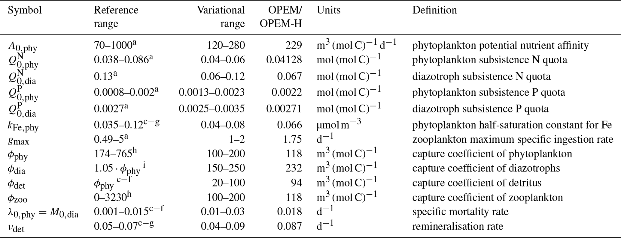
a Pahlow (2005), Pahlow et al. (2013). b Pahlow and Prowe (2010). c Keller et al. (2012). d Somes and Oschlies (2015). e Somes et al. (2017).
f Landolfi et al. (2017). g Landolfi et al. (2015). h Su et al. (2018). i Wang et al. (2019).
2.2.2 Likelihood-based metric assessing global biogeochemical model results
We consider four different types of observations for quantitatively assessing the model simulations. The first three are the objectively analysed monthly (upper 550 m) and annual (below 550 m) concentrations of nitrate, phosphate, and oxygen of the World Ocean Atlas 2013 (WOA 2013; Garcia et al., 2013a, b). The fourth is the monthly mean chlorophyll concentration derived from remote sensing data (MODIS Aqua level 3), based on monthly climatologies for 10 years from 2008 to 2017, provided by the ocean biology processing group (Ocean Biology Processing Group, 2014). The satellite-derived chlorophyll (Chl) concentrations are used for data–model comparison only for the UVic model's top layer, i.e. the upper 50 m.
We define our metric in terms of spatial averages of 17 distinct biogeochemical biomes, as derived and described by Fay and McKinley (2014). The individual biomes are regarded as regions of common biogeochemistry and thus account for spatial differences between ocean regions on the largest possible (global) scale. Using 56 biogeochemical provinces, as defined by Longhurst (2007), might have hampered our data–model comparison, because a higher resolution of individual regions can accentuate spatial pattern errors in tracer concentrations, resulting from model errors in advection and mixing. In our view, the biomes of Fay and McKinley (2014) are coarse enough for avoiding this problem but still sufficiently informative for identifying representative parameter values.
The underlying error model of the likelihood-based metric assumes a Gaussian (normal) distribution, which is well represented by using the first two moments of log-transformed tracer concentrations, in particular for the upper ocean layers (Schartau et al., 2017). For every depth level of the UVic model (), average log 10-transformed tracer concentrations () of type x are determined as spatial arithmetic means for our 17 biomes (indexed as j in Eq. 4) for the observations and model results:
where Njk is the number of available data points within biome j in depth level k. Prior to the log 10 transformation, all tracer concentrations have been normalised to lower detection (uncertainty) thresholds (x(0)), respectively. Measured or derived concentrations below these thresholds are treated as noise and therefore remain unresolved. Thus, the log 10-transformed normalised concentrations are non-negative. The threshold values are Chl(0)=0.1 mg m−3, mmol m−3, mmol m−3, and mmol m−3.
Our metric is derived from a likelihood, assuming a Gaussian error distribution for the residuals, which describes the discrepancy between mean values derived from observations () and model simulations (). Hereafter, we refer to this metric as our cost function (J). Our cost function is split up into two major parts:
where d is the residual vector (see Eq. 8 below), R the covariance matrix (Eq. 9), v(obs) and v(mod) are the spatial variance estimates of the log 10-transformed observed and modelled tracers, and V−1 are diagonal matrices with the variances (uncertainties) of v(obs). The first part () of the cost function resolves seasonal changes between the surface and 550 m depth, corresponding to the upper five depth levels of the model. The second part () represents the lower depth range below 550 m and does not account for seasonal changes, as only annual mean data are available.
The residual vector (d) (whose components represent the tracer types x) used for J describes the differences between the log 10-transformed observations and their model counterparts:
where i and j are the month and biome indices, respectively. We recall that d has four components only for the UVic model's top layer (k=1) where chlorophyll data are regarded as well. For k>1, the residual vector contains three components: O2, , and . Both parts of the cost function ( and ) in turn contain two terms, one with respect to the residuals, as defined in Eq. (8), and another that accounts for the differences between the spatial variances (vectors and ) within each biome (and month for ) at each depth level. The covariance matrices Rijk account for temporal correlations (Cjk) between different variables (x(obs)), that are specified for every biome and depth level separately:
where the elements of the diagonal matrices Sijk are the standard errors of the mean log 10-transformed tracer concentrations () calculated in Eq. (4) for every month i, biome j, and depth level k. For , the Rjk contain only the squared standard errors of the annual data as diagonal elements ().
With the consideration of standard errors instead of standard deviations, we implicitly impose weights to differences in the spatial expansion (i.e. number of data points of the gridded product used) of individual biomes. Overall, the final cost function J resolves spatial differences between regions (biomes) as well as temporal differences for those depth levels where monthly data are available. It is thus a combination of time-varying and spatial information for the assessment of our biogeochemical model results on a global scale.
In order to estimate uncertainty ranges for selected model results (globally averaged N2 fixation, , O2, DIC concentrations, NPP, NCP), we apply a bootstrap method to obtain an uncertainty quantification for our simulated values based on the 400 available ensemble model simulations. We collect the best solutions (lowest cost-function value) of 1000 randomly selected subsets of 100 out of our 400 ensemble members. The mean and 95 % confidence interval of these subsets provide an uncertainty range in the vicinity of the value of the full ensemble.
Table 2 lists the ranges of selected simulated tracers and processes for the full ensemble of parameter values generated by the Latin hypercube sampling for the OPEM and OPEM-H configurations. Our results exhibit wide ranges of tracer concentrations and fluxes in these two configurations. In particular, globally averaged concentrations range from 10.2 to 66.2 mmol m−3 and integrated N2 fixation from 0 to 515 Tg N yr−1. Tracers in OPEM and OPEM-H show similar ranges, except for globally averaged , which ranges from 10.2 to 66.2 mmol m−3 in OPEM and 13.0 to 55.0 mmol m−3 in OPEM-H.
Table 2Ranges of global averages of major tracer concentrations or fluxes in the OPEM and OPEM-H configurations. Chl concentration is for the upper 50 m (surface layer of the UVic grid) and NCP is for the upper 100 m. Observations and reference model simulations are listed in the Reference column.
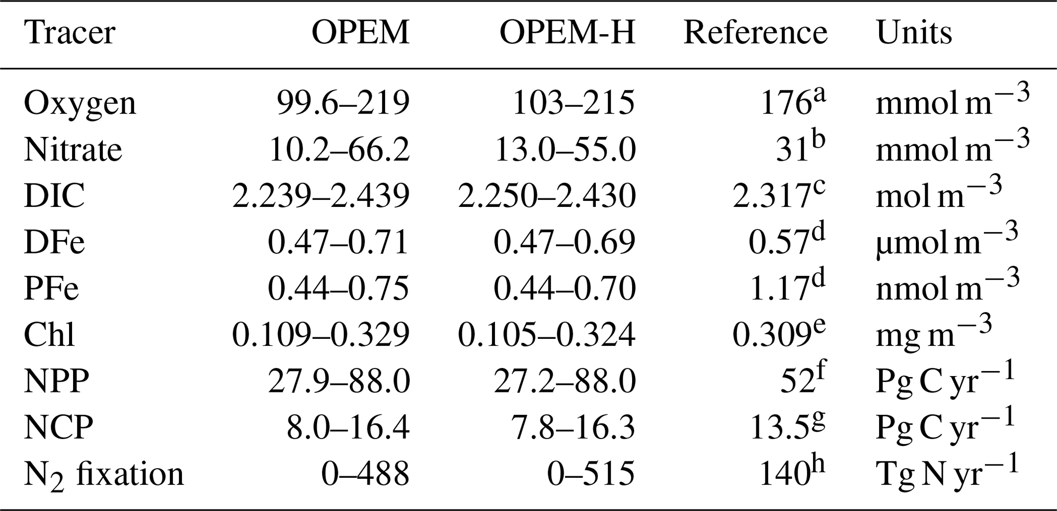
a WOA 2013 (Garcia et al., 2013a).
b WOA 2013 (Garcia et al., 2013b).
c GLODAPv2 (Olsen et al., 2016).
d Nickelsen et al. (2015).
e MODIS Aqua level 3, 2008–2017 (Ocean Biology Processing Group, 2014).
f Westberry et al. (2008).
g Li and Cassar (2016).
h Luo et al. (2012).
3.1 Sensitivity to model parameters
3.1.1 Biogeochemical tracer inventories and governing processes
The sensitivities of globally averaged biogeochemical properties to the variations of each of the 13 parameters in Table 2 are comparable for OPEM and OPEM-H (Fig. 1). Global mean oxygen concentration is most sensitive to νdet (remineralisation rate). Higher νdet increases oxygen consumption in shallow water, where oxygen resupply from the atmosphere is stronger. Less oxygen is consumed below the surface ocean; hence, the total oxygen inventory increases. Maximum ingestion rate (gmax) and grazing rate on ordinary phytoplankton (ϕphy) also correlate positively with oxygen. Higher gmax or ϕphy means more ordinary phytoplankton are grazed and less particles are formed, which then decreases oxygen consumption through remineralisation. Oxygen is less sensitive to ϕdia, because the biomass of diazotrophs is much smaller than that of ordinary phytoplankton.
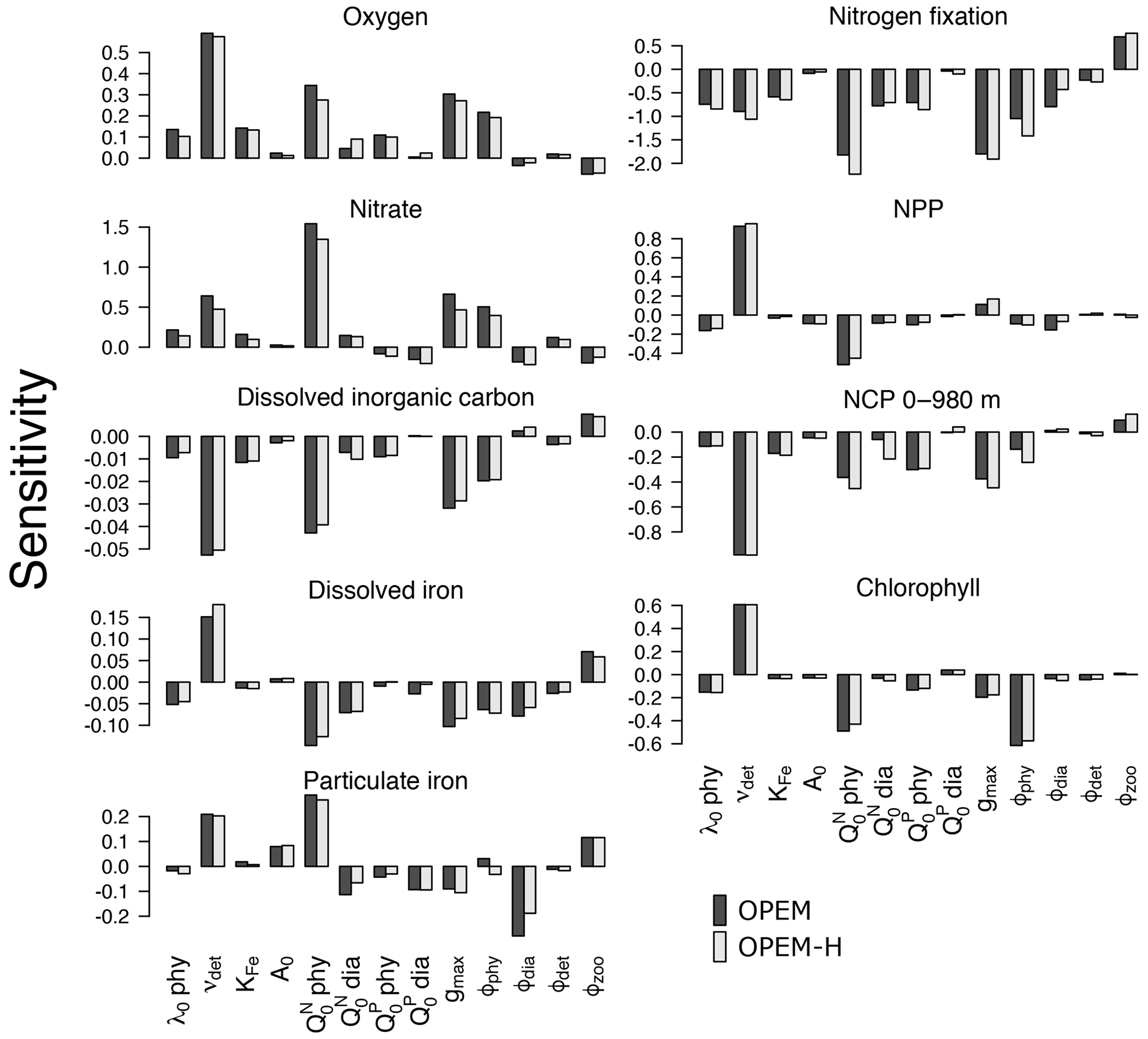
Figure 1Sensitivities of globally averaged O2, , dissolved inorganic carbon, dissolved iron, particulate iron, N2 fixation, NPP, chlorophyll, and NCP integrated from 0 to 980 m to individual model parameters, computed according to Eq. (3). Note the different y-axis ranges in the different panels.
A surprising finding is that oxygen is sensitive to, and positively correlated with, the subsistence nitrogen quota of ordinary phytoplankton (). From a classic point of view, oxygen levels in the ocean are dominated by physical supply processes as well as biogeochemical consumption processes such as remineralisation (Feely et al., 2004). Nevertheless, in our simulations, the sensitivity to is more than half (58 %) of that to νdet in OPEM and 48 % in OPEM-H (Fig. 1). In our model, has no effect on the spatial distribution of cellular C:N ratios in phytoplankton, which is determined by ambient light and nutrient conditions. However, affects the average phytoplankton C:N ratio. The average phytoplankton C:N ratio decreases when increases, with less carbon being fixed for the same supply. Oxygen consumption (due to remineralisation) per mole of nitrogen thus decreases in consequence. in turn affects : a higher yields a higher oxygen level and hence less denitrification in oxygen-deficient zones (ODZs) and therefore leads to more . In fact, we identify this as a major process that controls the inventory in our simulations (Fig. 1). While is also sensitive to other parameters, its sensitivity to is more than twice the sensitivity to any other parameter (Fig. 1).
The sensitivity of DIC is generally low, because of the relatively large DIC pool compared to the variations in fluxes among the different parameter sets. Similar to oxygen, DIC is most sensitive to νdet, , gmax, and ϕphy. Faster carbon recycling in the surface layer due to higher νdet generates a higher surface DIC concentration and hence more outgassing, which decreases the DIC inventory. A somewhat lower DIC inventory is also induced by a larger , as less carbon is fixed and exported per unit nitrogen in phytoplankton, and by enhanced zooplankton grazing with larger gmax.
Dissolved iron (DFe) is most sensitive to the remineralisation rate (νdet). Unlike , which has dynamic source (N2 fixation) and sink (denitrification) processes, iron has a fixed source from atmospheric deposition and a sink in the sediment, and the size of the DFe pool is mainly determined by its internal cycle. A higher remineralisation rate prolongs the residence time and thus increases the DFe pool. The parameter νdet also indirectly affects the internal DFe cycle via its effect on O2. While the detritus remineralisation rate drops when O2 falls below 5 mmol m−3 (Nickelsen et al., 2015), scavenging of DFe stops below the same oxygen threshold. Detritus remineralisation rate dominates variations in DFe when globally averaged O2 is above 135 mmol m−3, in which case DFe is positively correlated with νdet and O2. When globally averaged O2 is below 135 mmol m−3, the widespread ODZs (below 5 mmol m−3) inhibit the scavenging of DFe and this effect dominates. As a result, DFe becomes anti-correlated with O2. Particulate iron (PFe) is also positively correlated with νdet when globally averaged O2 is above 135 mmol m−3, but below that PFe shows no correlation with νdet. When globally averaged O2 is below 135 mmol m−3, inhibition of scavenging of DFe in ODZs decreases PFe there but a higher DFe increases PFe elsewhere, because PFe is coupled to DFe through scavenging and remineralisation. As mentioned above, controls the average nitrogen quota in phytoplankton and thus in particles. Since PFe is proportional to the amount of nitrogen in particles, also affects PFe. This (positive) sensitivity is much stronger than the indirect (negative) effect via DFe leading to opposite sensitivities of DFe and PFe to . Other than νdet and , PFe is also sensitive to ϕdia because dead diazotrophs enter the particulate pool (detritus) and diazotrophs are very sensitive to ϕdia (Fig. 2).
The simulated global N2-fixation rate is sensitive to many parameters, apart from A0,phy and . Similar relative changes in most parameters introduce changes to the global N2-fixation rate that are of similar magnitude. Interestingly, N2 fixation is sensitive also to zooplankton parameters, indicating that zooplankton grazing on diazotrophs is an important factor controlling not just diazotroph biomass but also N2 fixation.
Of particular interest are the sensitivities of global NPP and NCP. Particle fluxes in marine biogeochemical models tend to agree most closely with sediment trap data for depths of about 1000 m or below (Kriest et al., 2012). Therefore, different from Table 2, showing NCP for the upper 100 m for comparison with observations and other (reference) model simulations, here we integrate NCP from 0 to 980 m (7th layer of the ocean in the UVic-ESCM), which in steady state is equivalent to POC export flux at 980 m. NPP is sensitive to νdet and . A higher νdet causes faster nutrient recycling in surface waters, which increases NPP and reduces particle export and hence NCP. Increasing lowers both NPP and NCP, and hence also the fixed-carbon inventory. A higher ingestion rate of zooplankton (gmax) removes more particles and thus is negatively correlated with NCP. Chl is the principal agent of C fixation in the OPEM, and hence Chl has a similar sensitivity pattern to NPP except for gmax and ϕphy.
3.1.2 Ordinary phytoplankton, diazotrophs, particles, export, and their elemental stoichiometry
First, we discuss the proportions of carbon, nitrogen, and phosphorus in ordinary phytoplankton and diazotrophs, since variations in elemental stoichiometry in autotrophs originate in differential uptake of nutrients under different environmental conditions.
Globally averaged C, N, and P concentrations and ratios of globally averaged N and P of ordinary phytoplankton and diazotrophs are sensitive to νdet, , ϕphy, and ϕdia (Fig. 2). As expected, C, N, and P of ordinary phytoplankton and diazotrophs increase for higher νdet, which generates higher nutrient concentrations in the surface ocean. They are also sensitive to zooplankton grazing, especially to ϕphy and ϕdia. and are negatively correlated with ordinary phytoplankton C, indicating that the negative effect of higher subsistence quotas on competitive ability dominates their effect on biomass. A similar behaviour is found in diazotrophs except that is also negatively correlated with diazotroph N and hence also nitrogen fixation (Fig. 1). Although an increase in makes ordinary phytoplankton less competitive, it also raises the oceanic inventory, which eventually leads to more phytoplankton N (Fig. 2) and less nitrogen fixation (Fig. 1).
Diazotroph C, N, and P are generally more sensitive to parameter variations than phytoplankton due to the much smaller total biomass of diazotrophs, which is also the reason why diazotrophs are less sensitive in OPEM-H, the model configuration in which their biomass is generally larger because of the growth of diazotrophs at high latitudes (see Fig. 15 in Part 1; Pahlow et al., 2020). Since ordinary phytoplankton dominate autotrophic biomass, it tends to control nutrient distributions. This explains why ordinary phytoplankton parameters such as and ϕphy have strong effects on diazotrophs but not vice versa. The zooplankton grazing preferences ϕphy and ϕdia drive the competition between ordinary phytoplankton and diazotrophs and hence have strong and opposing effects on their biomass. Due to the relatively small total biomass, diazotroph C is more sensitive to changes in ϕphy and ϕdia than ordinary phytoplankton C.
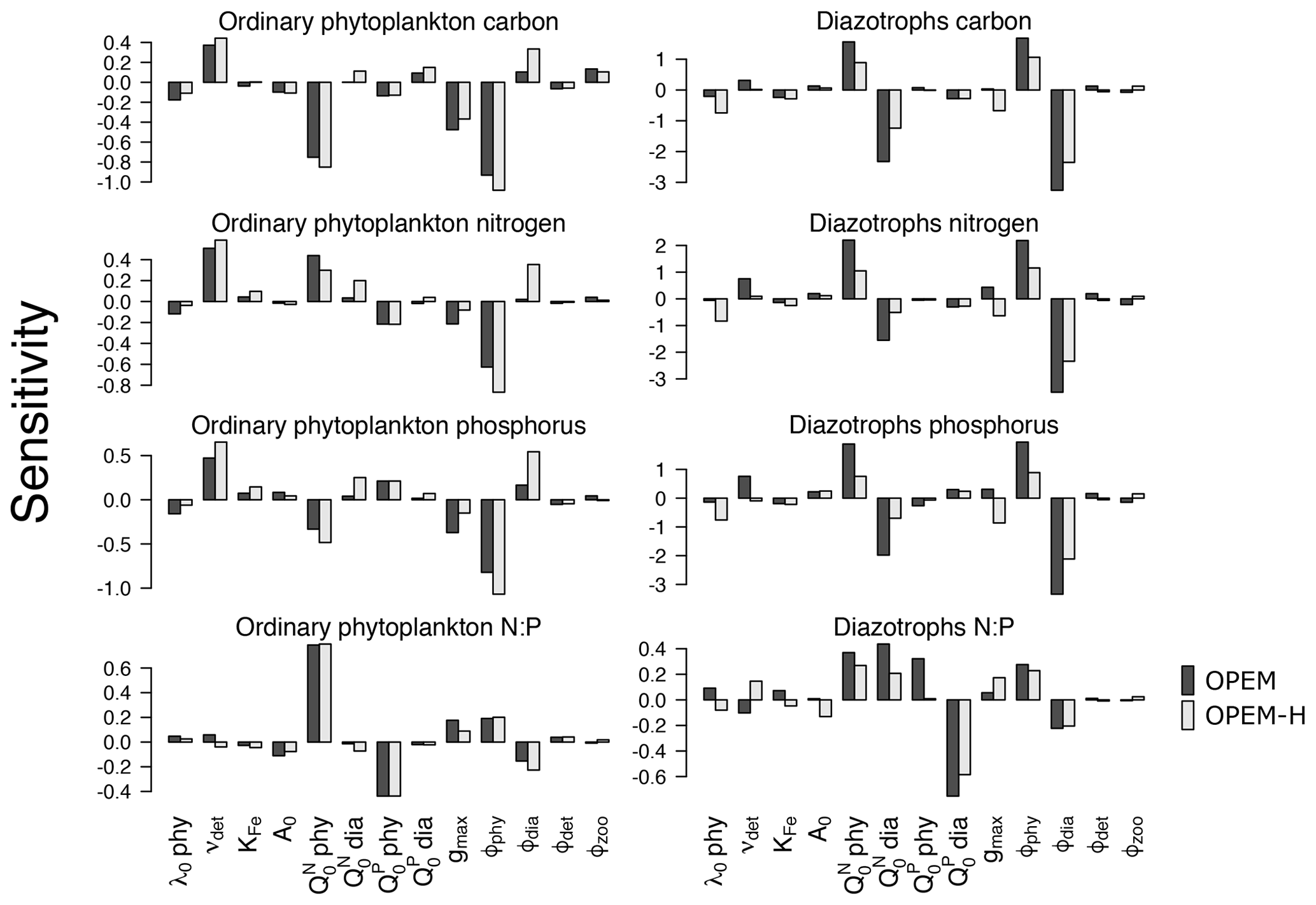
Figure 2Sensitivities of globally averaged concentrations of ordinary and diazotrophic phytoplankton C, N, and P, and ratios of globally averaged N and P to model parameters. Black and grey shading denotes OPEM and OPEM-H configurations, respectively. Note the different y-axis ranges in the different panels.
Particulate C:N and N:P ratios are most sensitive to (Fig. 3). This sensitivity is related to biomass, as we see from the OPEM-H configuration, where (non-N2-fixing) diazotrophs are abundant at high latitudes (see Fig. 15 in Part 1; Pahlow et al., 2020) and consequently the sensitivity of high-latitude C:N to is high, even higher than to (Fig. 3). We do not find this behaviour for high-latitude regions in the OPEM configuration, as well as low-latitude regions, where diazotrophs are not as abundant. The parameter was expected to be the most important parameter for particulate C:P ratios, just like is for the C:N ratio. However, this is only true for the OPEM at high latitudes.
At low latitudes, particulate C:P ratios are most sensitive to (Fig. 3). The supply of nitrate and phosphate at different latitudes is the major reason for this pattern. At low latitudes, the effects of are suppressed by variations in phytoplankton C, which is affected by and the consequent change in nitrate concentration. Nitrate and phosphate are not limiting in the high-latitude Southern Ocean, where, under N- and P-replete conditions, cellular C:P is mainly determined by and a higher would result in a higher cellular P:C (lower C:P). Therefore, the global C:P of total particulate matter, which is dominated by ordinary phytoplankton, is negatively correlated with .
The sensitivities of dissolved N:P ratio to parameters in the three geographical settings (low latitudes, high latitudes, and global) follow similar patterns. However, we find sensitivities to be generally higher in the low latitudes, especially to variations of the phytoplankton parameters. Again, this is because is often limiting in lower latitudes, particularly in the oligotrophic gyres, where the dissolved nitrogen pool is more sensitive to changes in phytoplankton as well as N2 fixation. This is also why grazing pressure on diazotrophs (ϕdia) has a much stronger effect at low than at high latitudes.
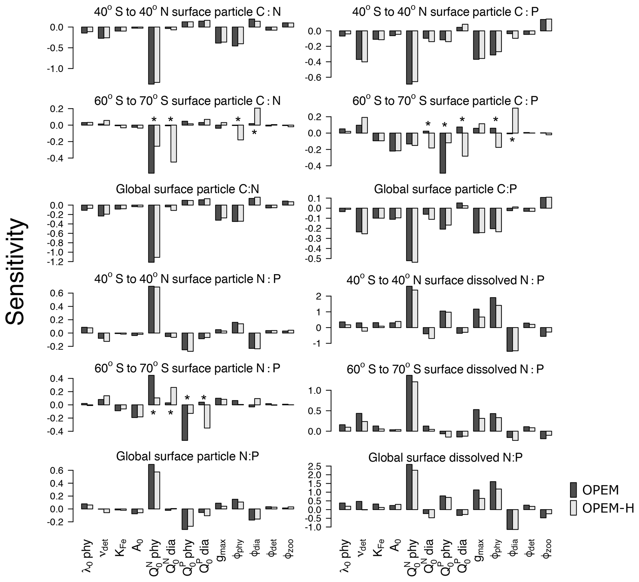
Figure 3Parameter sensitivities of averaged surface (0–130 m) particulate elemental C:N, C:P, and N:P ratios for different latitude bands (40∘ S to 40∘ N; 60∘ S to 70∘ S, and the global ocean). Asterisks indicate sensitivities that are very different between OPEM and OPEM-H. Note the different y-axis ranges in the different panels.
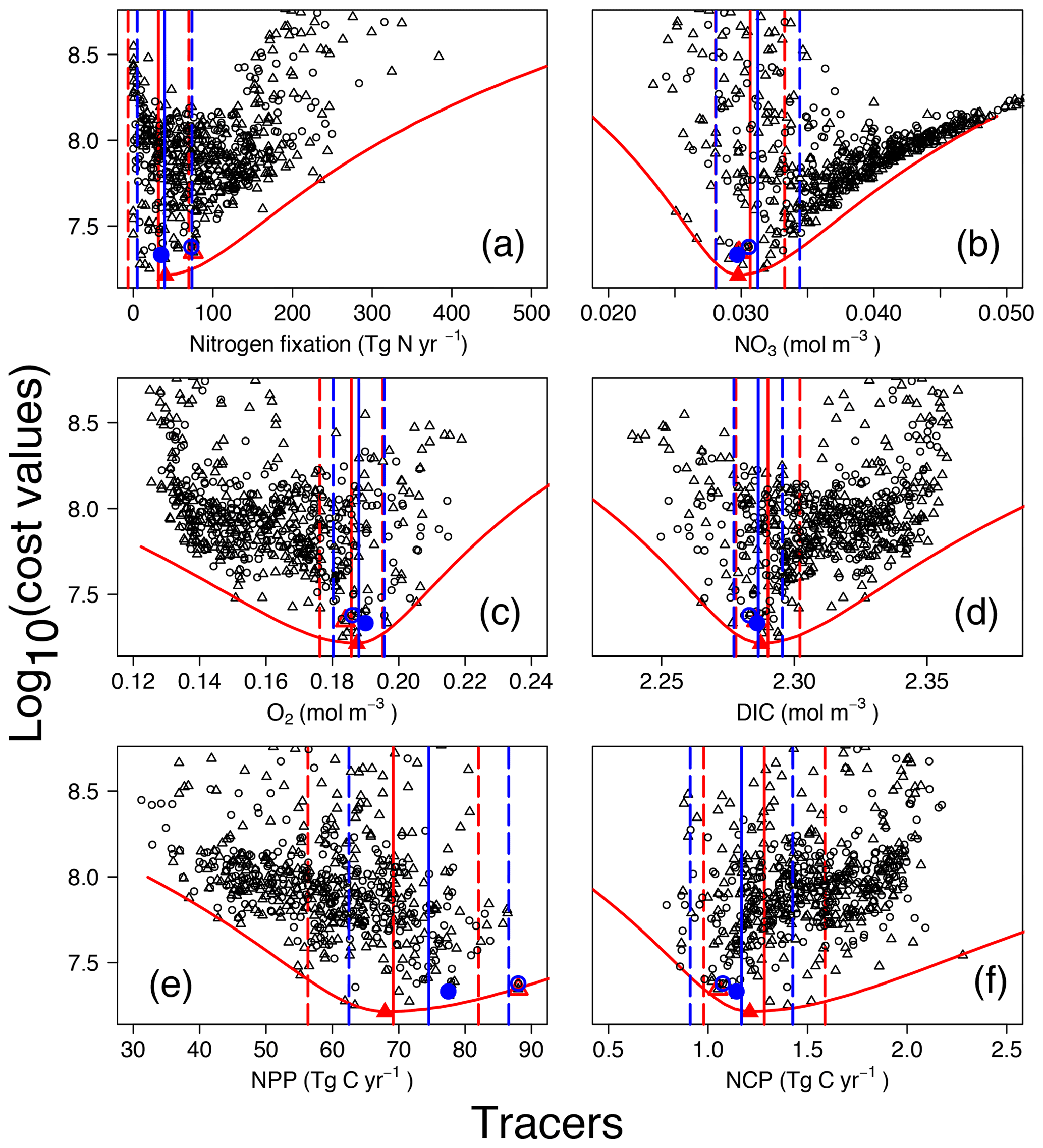
Figure 4Costs vs. tracer concentrations and fluxes for annual N2 fixation (a), globally averaged (b), O2 (c), and DIC (d) concentrations, as well as annual NPP (e) and NCP (here integrated over the depth range 0 to 980 m) (f). Red and blue symbols and lines are for OPEM (triangles) and OPEM-H (circles), respectively. Solid and open symbols represent minimum-cost and trade-off simulations, respectively. Vertical solid and dashed lines represent mean and 95 % confidence interval of best solutions of 1000 randomly selected subsets of 100 ensemble members. Red parabolas fit the lowest costs at different rates or tracer concentrations.
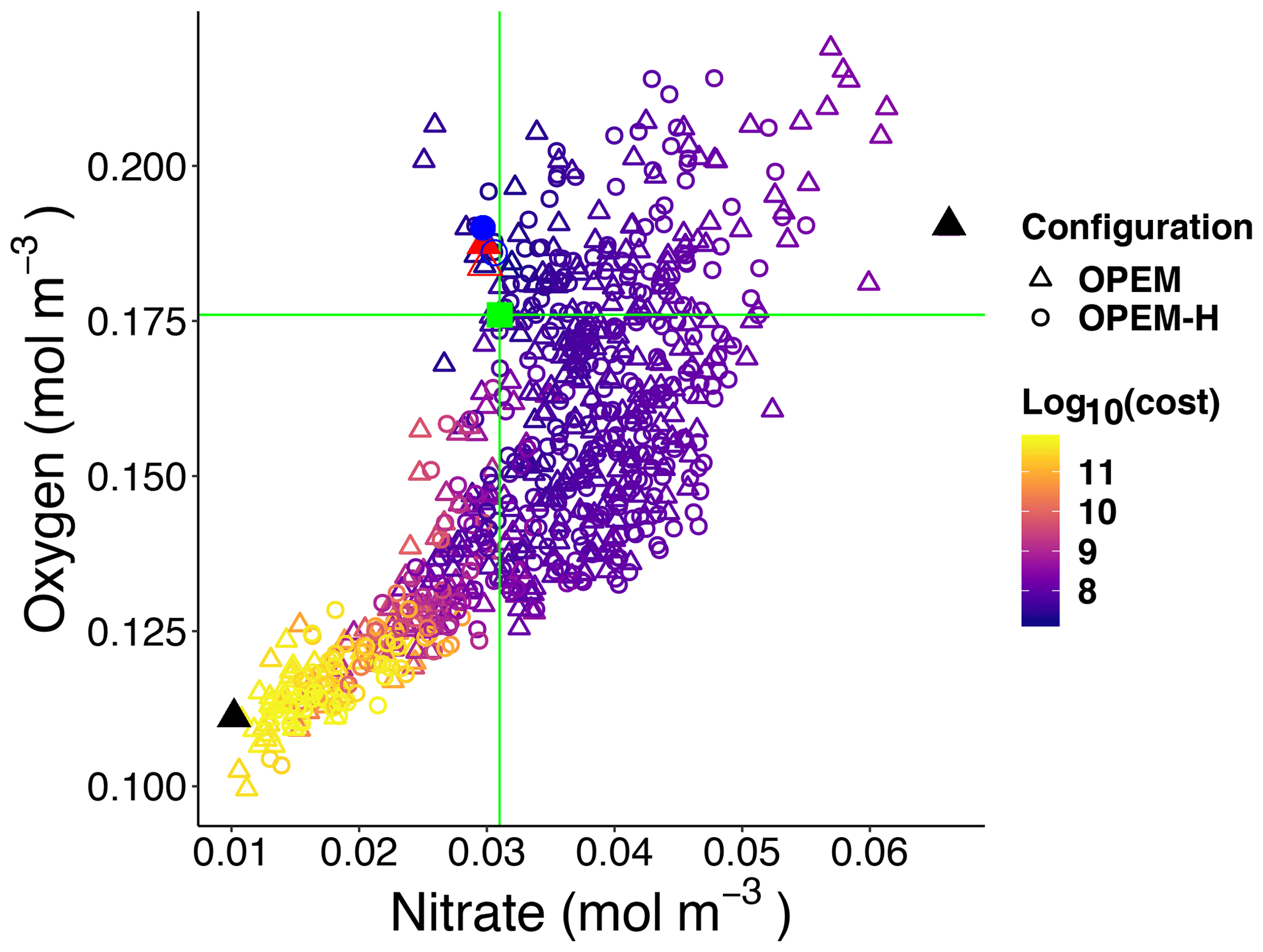
Figure 5Globally averaged oxygen vs. nitrate in OPEM and OPEM-H. Colour represents cost value. Solid red triangle and blue circle annotate the simulations with minimum cost in OPEM and OPEM-H, respectively, and open red triangle and blue circle are the trade-off simulations. The green square, horizontal and vertical lines indicate mean oxygen and nitrate concentrations of 0.176 and 0.031 mol m−3, respectively, in WOA 2013. Solid black triangles highlight the lowest and highest simulations used in Figs. 6 and 7.
3.2 Cost-function values of the ensemble simulations
3.2.1 Constraining global rate estimates and inventories
The cost function (introduced in Sect. 2.2.2) was devised for identifying the best solutions among the ensemble runs. For the model's upper layers (0–550 m), observational monthly mean concentrations of nitrate and phosphate enter the cost function, thereby reflecting regional and seasonal variations in the N:P uptake ratio of ordinary phytoplankton and diazotrophs. Variations in nitrate and phosphate availability affect the growth of diazotrophs and thus determine global N2 fixation in both OPEM and OPEM-H. In our UVic configurations, water-column denitrification is the only fixed-N loss term. Therefore, the simulated N2 fixation is expected to match water-column denitrification under a steady-state nitrogen cycle. Nevertheless, the simulation with the lowest cost yields a global N2-fixation rate estimate of 40.3 Tg N yr−1 (Fig. 4a), much lower than recent estimates of water-column denitrification (55.8–72.9 Tg N yr−1; Somes et al., 2017; Wang et al., 2019).
The cost function penalises solutions that yield N2-fixation rates greater than 90 Tg N yr−1 but shows no clear relation to N2 fixation at lower rates (Fig. 4A). For example, among the simulations with the five lowest cost-function values in the OPEM configuration, the global ocean N2-fixation rate varies between 8 and 40 Tg N yr−1. These model solutions also differ with respect to their O2 inventories. The tendency of the cost function to favour very low global N2 fixation is caused by a compensatory effect, whereby improving deteriorates O2, and vice versa (see also Part 1; Pahlow et al., 2020, and the discussion section below). Thus, instead of selecting the reference parameter sets based only on the cost function, we also take the ability to yield reasonable N2-fixation rates into account, whereby we ignore simulations with rates below 60 Tg N yr−1, since this is the lower boundary of current data-based estimates of water-column denitrification (DeVries et al., 2012). As these solutions represent a somewhat subjective trade-off between low cost and reasonable N2 fixation, we refer to them as trade-off solutions and details of their behaviour are shown and discussed in Part 1 (reference simulations in Pahlow et al., 2020). For OPEM, the trade-off solution corresponds to the seventh-lowest cost-function value and the fourth lowest for OPEM-H.
In the following, we will describe the lowest-cost solutions together with the trade-off solutions, as well as respective uncertainty ranges obtained from the bootstrap method described in the materials and methods section. The width of the uncertainty ranges (95 % confidence intervals) in Fig. 4 indicates the metric's ability to constrain the inventory or rate under consideration. Globally averaged N2-fixation rates of our trade-off solutions of OPEM and OPEM-H are just outside and within this uncertainty range, respectively (Fig. 4a). The global inventory turns out to be remarkably well constrained (Fig. 4b). The mean global estimates are 30.7 and 31.3 mmol N m−3 for OPEM and OPEM-H, respectively. Ensemble solutions that deviate from these estimates have high costs, and therefore the uncertainty ranges remain narrow. The trade-off and minimum-cost solutions are hardly distinguishable. The uncertainty of the simulated global O2 is comparable to that of the inventory. Global mean O2 concentrations of OPEM and OPEM-H are 186 and 188 mmol O2 m−3. Our metric effectively constrains global DIC estimates, 2.290 mol C m−3 for OPEM and 2.286 mol C m−3 for OPEM-H (Fig. 4d), although DIC data have not been explicitly considered in the cost function.
While the trade-off solutions exhibit , O2, and DIC inventories well within their respective uncertainty ranges, we find somewhat larger deviations for the predicted global mean NPP (Fig. 4e). For OPEM and OPEM-H, the trade-off solutions produce, respectively, 30 % and 14 % higher NPP than the minimum-cost solutions. The NCP (here integrated over the depth range of 0–980 m) estimates in Fig. 4F are better constrained than NPP for both configurations. The trade-off solution of OPEM corresponds to a global NCP of 1.05 Tg C yr−1, which is close to the trade-off estimate of OPEM-H, where NCP is 1.074 Tg C yr−1.
Figure 5 shows globally averaged concentrations of O2 versus of all ensemble members. The spread of the ensembles differs between the two tracers (by a factor of 2 for O2 and by a factor of 6 for ). Most solutions overestimate the global average concentration obtained from WOA 2013 (Garcia et al., 2013a, b) and underestimate O2. Solutions where both tracers strongly underestimate the WOA 2013 data are penalised by the cost function (Fig. 5). The minimum-cost and trade-off solutions of OPEM and OPEM-H are close to the WOA 2013 estimates. The respective optimal solutions have slightly higher global mean O2 concentrations than WOA 2013 and are in good agreement with respect to . In spite of larger costs, the trade-off solutions of both OPEM and OPEM-H are closer to the WOA 2013 estimate than the minimum-cost solutions (Fig. 5). The ensemble solutions are unevenly spread around the WOA 2013 data-based estimates. This highlights that our trade-off solutions could not have been identified had we only considered the ensemble means.
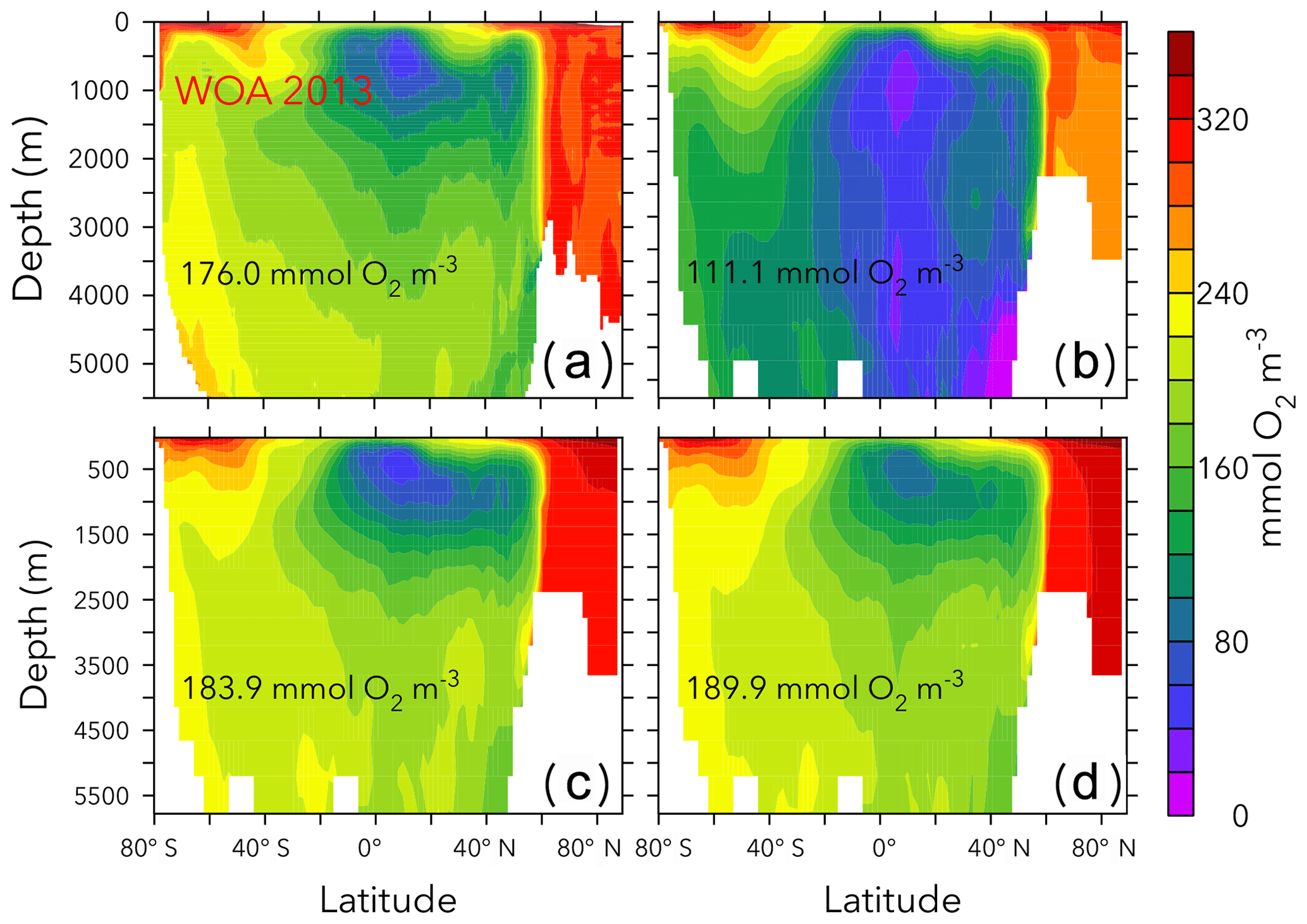
Figures 6 and 7 show zonally averaged and O2 in simulations with the lowest and highest and the trade-off simulation in the OPEM configuration. The high- simulation has similar and O2 patterns to the trade-off simulation, despite the very different mean and O2 concentrations. The patterns are different in the low- simulation because of stronger deoxygenation and denitrification, which occur mostly in North Pacific deep water. The greater similarity of global mean O2 than reflects the influence of atmospheric O2 but also indicates that is more sensitive to changes in the physiology of the diazotrophs.
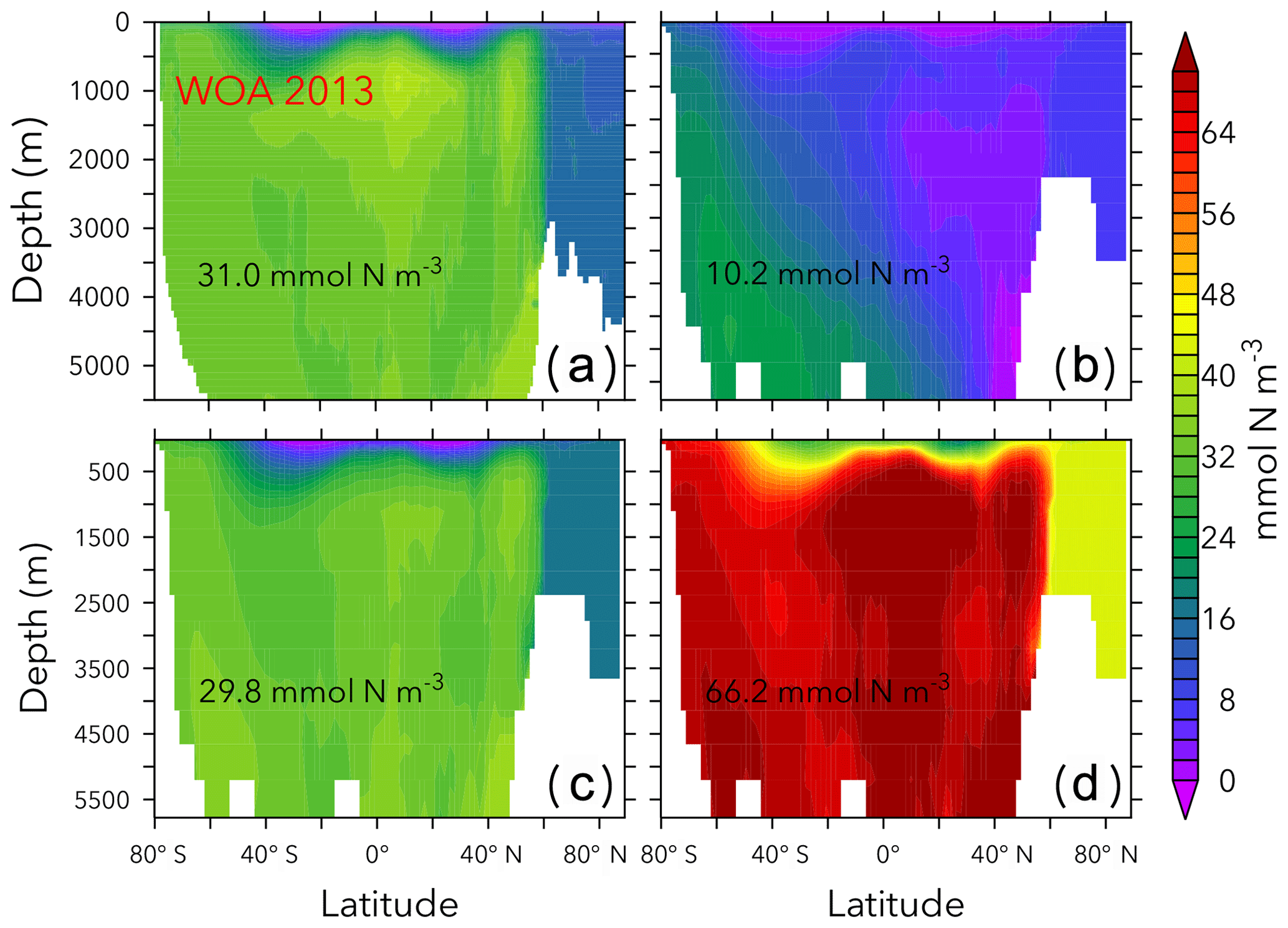
Figure 6Zonally averaged in WOA 2013 (a), the simulations with the lowest and highest inventory (b, d), and the trade-off simulation (c) in the OPEM configuration. Globally averaged concentrations are shown in each panel. Simulations shown here are marked with solid black and open red triangles in Fig. 5. Note that the outputs from OPEM and OPEM-H are very similar and only OPEM results are shown here.
3.2.2 How well can model parameters be constrained?
Cost is conspicuously correlated only with νdet, , and ϕdia (Fig. 8). O2 and are sensitive to νdet and but not to ϕdia (Fig. 1), which indicates that ϕdia becomes more important at lower-cost simulations. The minimum-cost and trade-off simulations in OPEM and OPEM-H are usually closer to each other when parameters show strong correlations with costs (Fig. 8).
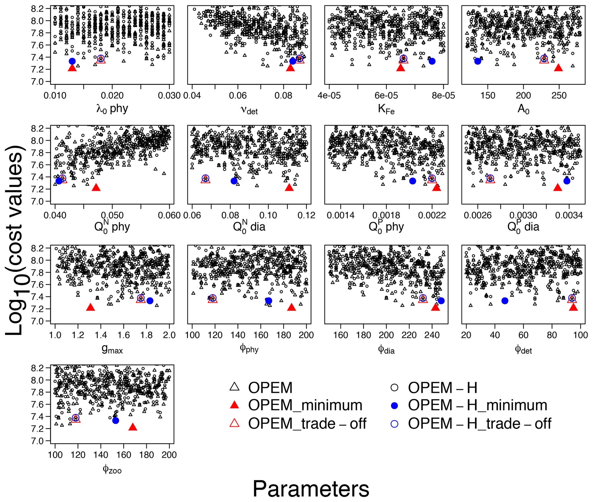
Figure 8Lower parts (cost<108.2) of cost–value distributions for the parameter ranges in Table 1. Solid red triangles and blue circles represent the minimum-cost simulations in OPEM and OPEM-H, respectively, and open red triangles and blue circles are the trade-off simulations. Note that the trade-off simulations share the same parameter combination but have slightly different cost–value distributions.
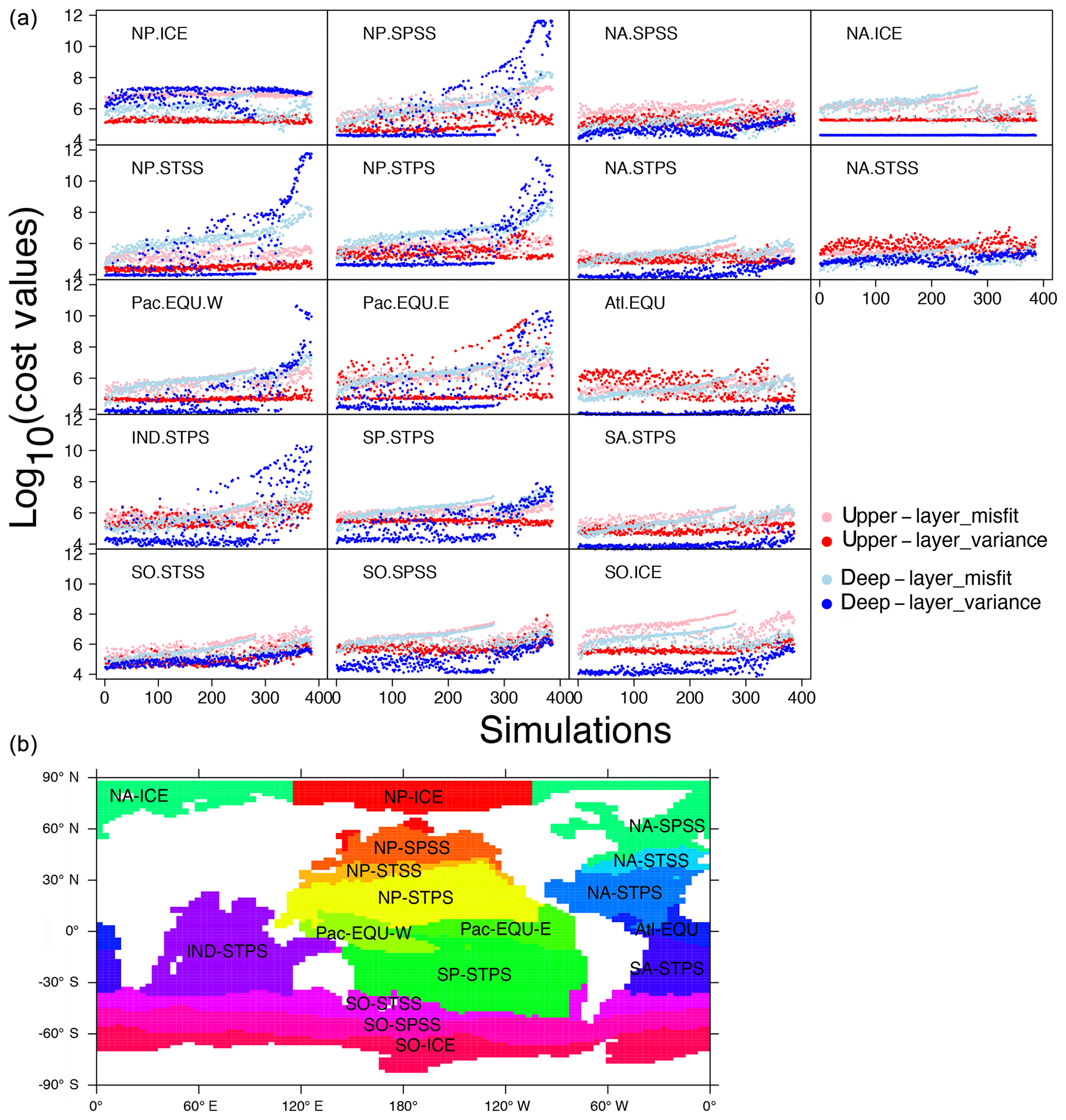
Figure 9(a) Cost–value distributions in the 17 biomes in OPEM. The order of the simulations is based on the total cost from low to high in OPEM. The upper layer and deep layer in the legend represent upper (0–550 m) and lower (below 550 m) components of the cost function (Eq. 5). Misfit and variance are calculated by the first and second parts of the cost-function components (Eqs. 6 and 7), respectively. (b) Map of biome locations.
Figure 9 shows how different biomes contribute to the misfit and variance parts of the total cost. For simulations with high cost-function values (J>1010), we find the variance term to be dominant in the deep ocean (below 550 m). Among the 17 biomes, this is well expressed in the NP.SPSS (North Pacific subpolar seasonally stratified), NP.STSS (North Pacific subtropical seasonally stratified), NP.STPS (North Pacific subtropical permanently stratified), Pac.EQU.E (eastern Pacific equatorial), Pac.EQU.W (western Pacific equatorial), and IND.STPS (Indian Ocean subtropical permanently stratified) biomes, overwhelming contributions from all other parts of the cost function and all other biomes for the 100 simulations with the highest total costs. These high-cost simulations tend to have low and O2 concentrations (Fig. 5). Low concentrations are coupled to low O2 because of intense denitrification in the ODZs. Accordingly, simulations with very low inventories suffer from widespread ODZs, occupying much of the deep water in the northern and equatorial Pacific as well as the Indian Ocean (Fig. S1 in the Supplement). This is the main reason for the high variance in the deep water of these biomes (Fig. 9).
4.1 Parameter sensitivities
4.1.1 Remineralisation rate νdet and phytoplankton subsistence nitrogen quota
Remineralisation rate (νdet) and phytoplankton subsistence nitrogen quota () are the two parameters with the strongest correlations for most tracers as well as particulate elemental stoichiometry. The importance of νdet was expected, because it is an important driver of nutrient recycling in the surface ocean (Thomas, 2002; Anderson and Sarmiento, 1994; Eppley and Peterson, 1979), which strongly affects NPP, NCP, Chl, DIC, DFe, and N2 fixation (Kriest et al., 2012). νdet also determines the rate of O2 consumption, hence also the level, due to denitrification in ODZs (Cavan et al., 2017). The strong influence of , however, was unexpected. The subsistence quota was first introduced by Droop (1968) in phytoplankton growth models. While it has been applied in Earth system models (Kwiatkowski et al., 2018; Wang et al., 2019), a sensitivity analysis similar to the present study has not been done before. A higher implies that more nitrogen is required for phytoplankton growth, but it also can be interpreted as a lessening of carbon fixation for a given nitrogen supply. Our results demonstrate a strong effect of on NPP, Chl, and POC export (NCP, here integrated over the depth range 0 to 980 m), and consequently oxygen consumption and denitrification.
These results also put forward a new point of view on the relation between inventory and carbon export. In classic biogeochemistry, a larger inventory in the ocean stimulates primary production and POC export. This feedback is intuitive and easy to understand, as for a given C:N in phytoplankton, carbon is proportional to the nitrogen pool. This feedback is well recognised and has been widely applied in marine sciences, especially since it forms the foundation of one of the hypotheses explaining the lower atmospheric pCO2 during the Last Glacial Maximum (LGM) (McElroy, 1983; Falkowski, 1997). However, our analysis of the model ensemble with different parameter combinations suggests another, very different, point of view. concentration is positively correlated with but negatively with NPP and POC export (NCP; Fig. 1), which means that an increased inventory can be related to a lower POC export if caused by a change in . The dynamic C:N ratio in our model explains part of this negative correlation. When the inventory increases due to an increase in , the nitrogen demand in phytoplankton also increases, which yields a lower C:N ratio in phytoplankton, and hence changes in carbon fixation due to increases in inventory remain relatively small. The increase in increases nitrogen in phytoplankton structure and decreases the C:N ratio in phytoplankton as well as detritus. The two effects together both lower POC production and raise the inventory. Changes in νdet also contribute to the negative correlation between and POC export (NCP) in our simulations: a more intense remineralisation in the surface ocean reduces POC export and thus decreases oxygen consumption and denitrification, resulting in a larger nitrate inventory.
The strong impact of on the inventory and globally averaged phytoplankton C:N causes a higher sensitivity of globally averaged C:N than C:P (Fig. 3). A higher results in a higher inventory and a lower phytoplankton C:N, both tending to lower particulate C:N, and vice versa. On the other hand, C:P is not as sensitive because we have a constant inventory in the UVic model. Surface particulate matter C:N is less variable compared to C:P and N:P in field observations along regional gradients (Galbraith and Martiny, 2015; Geider and Roche, 2002; Martiny et al., 2013a; Sterner and Elser, 2002), which is an apparent contrast to our results, where the sensitivity of C:N to is the highest among the particulate elemental ratios. However, our sensitivities are with respect to parameter variations among many simulations, rather than spatial or temporal gradients in the one real ocean.
4.1.2 Zooplankton parameters
While in many global biogeochemical models zooplankton are described by non-mechanistic formulations, such as Holling-type functions (Holling and Buckingham, 1976), in this study we apply a more realistic zooplankton model (Pahlow and Prowe, 2010). Among the five zooplankton parameters, the maximum specific ingestion rate (gmax) and the capture coefficients of phytoplankton (ϕphy) and diazotrophs (ϕdia) are the most important, whereas the preference for detritus (ϕdet) is generally less important. Grazing on zooplankton itself (ϕzoo) counters the effect of gmax because it lowers zooplankton biomass and thus total ingestion. These parameters together dominate controls on N2 fixation and Chl (Fig. 1), and C, N, and P of ordinary phytoplankton and diazotrophs (Fig. 2). It is interesting that zooplankton parameters also exert some control on particulate N:P as well as the dissolved nutrient pools (Fig. 3). This can be understood via their controls on N2 fixation and the ensuing changes in N:P in the dissolved and particulate pools.
4.1.3 Other parameters and the OPEM-H configuration
Other parameters in the sensitivity analysis appear less important for the tracer distributions, but this does not necessarily mean that they are negligible. Specific mortality rate (λ0,phy) and the phytoplankton half-saturation constant for Fe (kFe,phy) do contribute to some variations of most of the tracers (Fig. 1), and particulate C:P is somewhat sensitive to potential nutrient affinity (A0). Phytoplankton subsistence P quota () affects major tracers much less than phytoplankton subsistence N quota (), but it is still important for particulate C:P and particulate N:P ratios, particularly at high latitudes and globally (Fig. 3). Diazotroph subsistence N and P quotas ( and ) in general have much less influence on particulate stoichiometry than and because diazotrophs are much less abundant than ordinary phytoplankton. However, diazotroph biomass (carbon) itself is more sensitive to than , which shows that the diazotroph subsistence quotas are still important for both their elemental stoichiometry and ability to compete with ordinary phytoplankton. While elemental stoichiometry has been suggested to be an important factor for determining the outcome of the competition between diazotrophs and non-diazotrophs, and consequently N2 fixation (Deutsch and Weber, 2012; Weber and Deutsch, 2012), we find that N2 fixation is no more sensitive to than to the remineralisation rate (νdet), , or zooplankton grazing parameters (gmax, ϕphy, and ϕdia). Nevertheless, our analysis agrees with the argument that global N2 fixation is mainly determined by rates of fixed-N loss (Weber and Deutsch, 2014), which in our model is largely affected by νdet and .
In general, tracer sensitivities to parameters in OPEM-H configuration are similar to those in OPEM. O2 and levels are slightly less sensitive to the remineralisation rate, , and gmax in OPEM-H because this configuration allows (facultative) diazotrophs to grow in high-latitude cold waters; hence, the overall biomass of diazotrophs is greater (Part 1; Pahlow et al., 2020). This is also the reason why and exert a stronger effect on surface-particle elemental stoichiometry at high latitudes in OPEM-H (Fig. 3).
Several studies have revealed that N2 fixation occurs in high-latitude regions (Sipler et al., 2017; Harding et al., 2018; Shiozaki et al., 2018; Mulholland et al., 2019), which supports a wider temperature range of N2 fixation, similar to what we have in OPEM-H. In the trade-off simulation for OPEM-H, we do find some N2 fixation in the eastern North Pacific and the Arctic Ocean (Part 1; Pahlow et al., 2020). The different temperature function for diazotrophy is also the reason for the differences in the sensitivities of particulate to diazotroph subsistence quotas in high-latitude regions (Fig. 3).
4.2 Model limitations
The strong correlation between O2 and (Fig. 5) indicates that O2 and denitrification are tightly coupled. Lack of benthic denitrification leaves water-column denitrification as the only loss of and O2 becomes the primary factor controlling the inventory. This implies that sensitivities of to the model parameters could be different when benthic denitrification is incorporated in our model. Also, this means that global N2 fixation (same as global denitrification in our spun-up steady-state simulations) is underestimated, and since it occurs mostly at 40∘ S to 40∘ N (see Fig. 13 in Part 1; Pahlow et al., 2020), particulate carbon to nitrogen (C:N) ratios could be overestimated due to a missing input of nitrogen to the surface ocean. This could explain the overestimated surface particulate C:N at low latitudes (see Table 3 and Fig. 16 in Part 1; Pahlow et al., 2020).
To evaluate how water-column denitrification affects our cost function, we arrange our simulations in the order of their cost values and plot the volume of ODZs against cost for both the OPEM and OPEM-H configurations in Fig. 10a–c. Several of our simulations, mostly among those with the 200 lowest cost values (Fig. 10a), have a relatively small misfit in O2 and compared to the WOA 2013 estimate, and high N2-fixation rates, comparable to those estimated in previous model studies (e.g. Somes et al., 2017; Wang et al., 2019). For these simulations, low O2 is connected with high rates of water-column denitrification in the eastern equatorial Pacific Ocean (Pac.EQU.E), causing a depression of concentration and a rather high variance in concentration, both of which conflict with the observations. Hence, cost in this biome is very high, especially in the upper 550 m (Fig. 9), where denitrification is strongest. On the other hand, although the volume of ODZs in the minimum-cost simulations in OPEM and OPEM-H is greater than in WOA 2013 (Fig. 10c), they yield rather low N2-fixation rates (40.3 and 35.0 Tg N yr−1 for OPEM and OPEM-H, respectively). ODZ volumes in the trade-off simulations are more than twice that in WOA 2013 (Fig. 10) and yield global N2-fixation rates close to current estimates of water-column denitrification (about 70 Tg N yr−1; Somes et al., 2017; Wang et al., 2019). The mismatch between ODZ volume and N2-fixation rate indicates that a refined description of water-column denitrification may be needed (Sauerland et al., 2019). While the physical component (ocean circulation) of the UVic model is also very important for the global distribution of oxygen and nitrate, our results suggest that, clearly, only by considering all major nitrogen sources and sinks, such as atmospheric deposition and benthic denitrification, a better representation of N2 fixation and the global marine nitrogen cycle can be achieved.
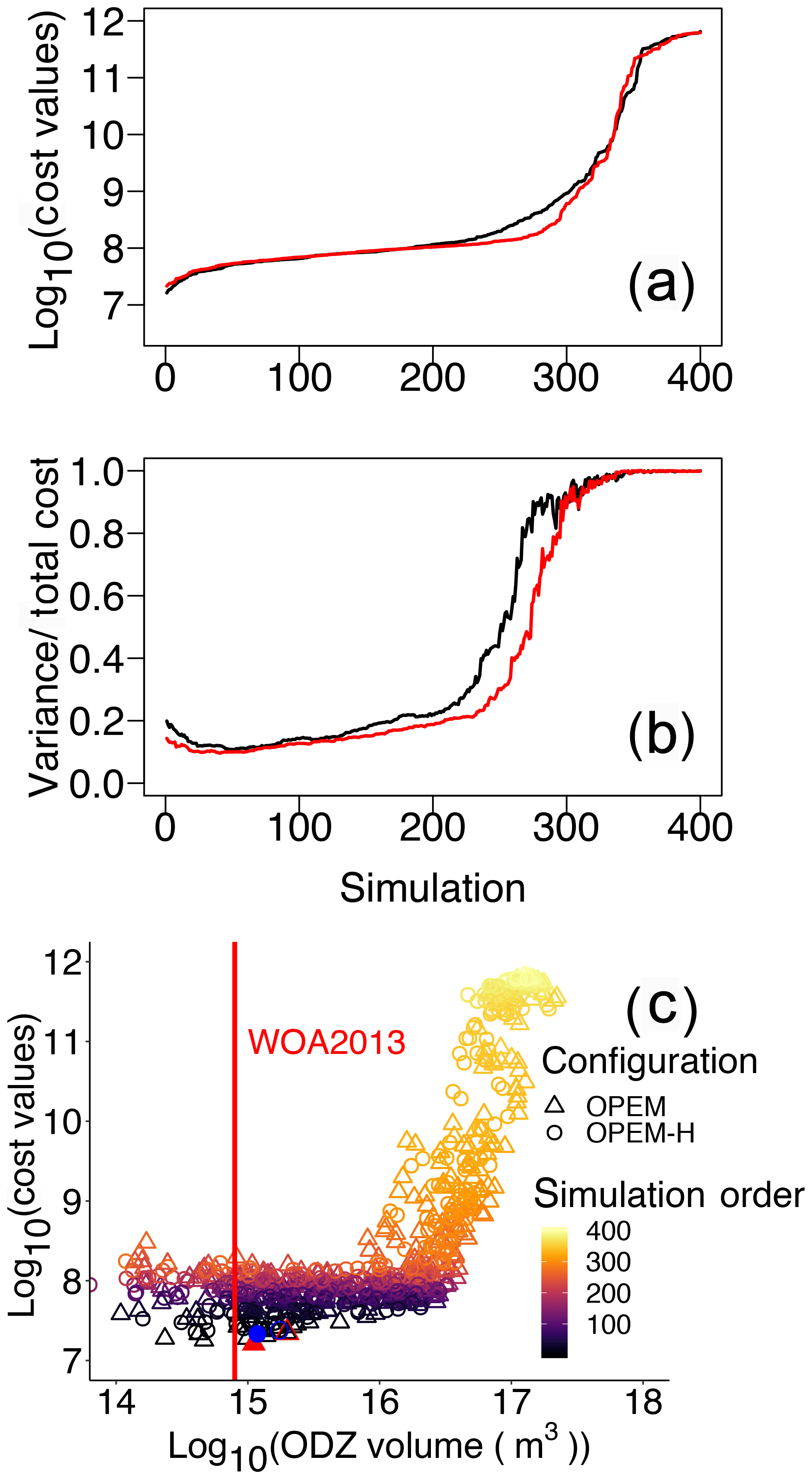
Figure 10Cost values across all parameter sensitivity simulations ordered from low to high for the two model configurations. Cost values in both misfit and variance (a) and the contributions of variance (b). Black and red lines are for OPEM and OPEM-H, respectively. Total cost versus volume of ODZ (ODZ <5 mmol O2 m−3) in the simulations with ODZ volume larger than 1014 m3 (c); colour represents the simulation order as shown in panels (a) and (b). The red vertical line indicates ODZ volume in WOA 2013 (7.945×10¹⁴ m3), the solid red triangle and blue circle represent the simulations with minimum cost in OPEM and OPEM-H, respectively, and open red triangle and blue circle are the trade-off simulations.
4.3 Likelihood-based metric
4.3.1 Applicability of the cost function and usefulness of introducing variance information
The cost function introduced above is a metric that quantifies the discrepancy between objectively analysed observational data and simulation results. Our cost function proves useful for exploring the 400 ensemble model solutions and identifies model solutions that reproduce deep ocean gradients in the ratio better than a classic fixed-stoichiometry model (Part 1; Pahlow et al., 2020). In addition, the optimal model solutions yield improved NCP rate estimates integrated over the top 100 m (Part 1; Pahlow et al., 2020). In particular, the trade-off solutions of OPEM and OPEM-H can resolve observed latitudinal patterns in dissolved and particulate within the upper productive ocean layers (0–130 m; see Part 1; Pahlow et al., 2020). The consideration of monthly mean O2, , data for the upper 550 m and surface Chl remote sensing data introduces important constraints on the representation of the relation between light and nutrient limitation, thereby also specifying the degrees of N and P limitation.
Even within the 5 % of the simulations with the lowest costs, the estimates of global N2-fixation rate vary considerably. The mean global estimates ± standard deviation in OPEM and OPEM-H are 32±20 and 39±18 Tg N yr−1, respectively. We initially expected that the and data in the cost function would effectually constrain N2 fixation. This is clearly not the case and additional information has to be considered. One explanation may be that considerable N2 fixation can occur during short periods and may also be confined to regions smaller than the biomes. Regional differences with respect to N2 fixation remain unresolved if only biome-specific monthly mean and data are considered for the upper layers in the cost function.
Also, the minimum-cost solution yields very low global N2-fixation rates. Thus, for the identification of the trade-off solutions, we had to consider prior information about global water-column denitrification, whose rate is balanced by N2 fixation according to our models. Incorporating N2 fixation as a single global rate estimate into our Likelihood-based cost function as a single additional term would, without some difficult-to-define regularisation, become overwhelmed by the many tracer and variance terms defined in Eqs. (6) and (7). Rather, the additional information is treated as a second objective, namely that global N2 fixation should be greater than 60 Tg N yr−1 (see above), which is similar to applying a multi-objective approach for model calibration (e.g. Sauerland et al., 2019), where a trade-off between two or more objectives (cost functions) is resolved. A refined cost function may incorporate monthly mean N:P ratios or N* values based on WOA 2013 data (e.g. for the upper 130 m) for clustered subregions of some biomes. Such addition to the cost function would require some careful preprocessing, e.g. cluster analysis of the spatial N:P or N* patterns but may suffice to constrain simulated N2-fixation rates.
A peculiarity of our cost function is that it complements the data–model misfit, i.e. the residuals of spatial mean log 10-transformed values, with an additional term that resolves differences in spatial variances. How the neglect of this term affects the global mean tracer concentrations and flux estimates is depicted in Fig. S2–S7 in the Supplement. The cost function's variance term introduces a strong penalty to approximately 30 % of all ensemble model solutions. The highest cost-function values (J>109) are associated with discrepancies in spatial variances that exceed the misfits in the log 10-transformed tracer concentrations. For large parts of the ensemble solutions, the variance term contributes between 15 % and 20 % to the total costs. Interestingly, for those model solutions that yield low cost-function values (), the relative contribution rises again when the misfit in the log 10-transformed tracer concentrations gradually decreases (Fig. 10b).
4.3.2 Contributions of biomes
The 17 biomes derived by Fay and McKinley (2014) represent a scale similar to that addressed in global efforts to establish surface–ocean air–sea carbon-flux estimates (Wanninkhof et al., 2013; Rödenbeck et al., 2015). Accordingly, our cost function can be easily extended by incorporating air–sea CO2 flux estimates in the future. Further improvements may be possible by introducing subregions in some biomes, e.g. for constraining N2-fixation rate estimates, as discussed above.
For low cost-function values, the contribution of the variance term is generally small in most biomes for the deep layers (Fig. 9), where variances of the log 10-transformed tracer concentrations compare very well between the simulations and the WOA 2013 estimate. For high costs, this term can become dominant, e.g. for some biomes in the North Pacific as well as the Indian Ocean. A remarkable exception is the North Pacific Arctic biome (NP-ICE), where the deep layer's variance term remains dominant for most of the ensemble solutions. This is somewhat different in the Arctic biome of the North Atlantic (NA-ICE) and the Southern Ocean (SO-ICE), where the variance term remains low throughout almost the entire ensemble. For SO-ICE, the cost function is mainly affected by the misfit in log 10-transformed tracer concentrations. The misfit is associated mainly with discrepancies between observed and simulated within the SO-ICE biome. Interestingly, these misfits in both upper and deeper layers drop again after around the 280th simulation. Simulations with high do not result in total cost values as high as in simulations with very low (Fig. 5), but they have larger misfits for in SO-ICE. A similar behaviour can be seen in the other Southern Ocean biome (SO-SPSS) as well as in NA-ICE.
The upper layer's variance term contributes strongly to low costs in North Atlantic biomes. This is particularly striking for the equatorial Atlantic biome (Atl.EQU). The main reason is water-column denitrification that results in a high variance in . Likewise the eastern equatorial Pacific biome (Pac.EQU.E) reveals major model limitations in the upper layers. Overall, the unfolding of biome-specific contributions to the cost function clearly points to those regions where improving model performance appears most worthwhile. Our present cost function may then be reapplied to quantify and highlight specific model improvements.
We demonstrate sensitivities of various tracers and processes to parameters in two configurations of a new optimality-based plankton–ecosystem model (OPEM) in the UVic-ESCM. While OPEM-H predicts a wider geographical range for N2 fixation (Part 1; Pahlow et al., 2020) and shows some differences in the sensitivities of diazotroph C, N, and P to parameters when compared to OPEM, the tracer sensitivity to model parameters is very similar in both configurations. The trade-off simulations in the OPEM and OPEM-H happen to have the same parameter set. Among our model simulations, varying model parameters within reasonable ranges results in variations in O2 by a factor of 2 and in concentration by a factor of 6. The sensitivity analysis provides important information regarding the new models' behaviour. The O2 inventory is mainly influenced by the remineralisation rate (νdet) as well as phytoplankton subsistence nitrogen quota () and zooplankton maximum specific ingestion rate (gmax). Changes in strongly impact the inventory, as well as the elemental stoichiometry of ordinary phytoplankton, diazotrophs, and detritus. also affects N2 fixation, Chl, DIC, and iron levels. Furthermore, our sensitivity analysis resolves correlations between various biogeochemical tracers. For example, POC export is negatively correlated with the inventory. We would like to point out that these changes in model behaviour are solely caused by variations in parameters. Thus, the correlations between tracers and rates might not stand when tracer variations are caused by other factors. For example, an increase in the inventory due to anthropogenic emissions may be accompanied by an increase in POC export (Fernández-Castro et al., 2016). Also, although we did evaluate sensitivities of particulate elemental stoichiometry at different latitudes, most tracer sensitivities and correlations should be considered valid only for global but not regional scales.
We introduce a new likelihood-based metric for model calibration. The metric appears capable of constraining globally averaged O2, , and DIC concentrations as well as NCP. In particular, the minimum-cost and trade-off model solutions resolve observed latitudinal patterns in particulate within the surface layers (0–130 m). However, the metric does not effectually constrain the models' global N2-fixation rate estimates. Individual contributions of the biomes to the cost function provide details of how tracer distributions in each biome respond differently under different ecosystem settings. The consideration of spatiotemporal variations in the stoichiometry of , , and O2 in our metric favours model solutions with low N2-fixation rates that are solely balanced by low rates of water-column denitrification. From our findings, we conclude that an explicit consideration of benthic denitrification and atmospheric deposition seems critical for improving the representation of the complete global nitrogen cycle in our model.
The University of Victoria Earth System Climate Model version 2.9 (original model) is available at http://www.climate.uvic.ca/model/ (last access: 17 September 2020). The OPEM v1.1 code is available at https://doi.org/10.3289/SW_1_2020 (Pahlow, 2020). The instructions needed to reproduce the model results described in this article are in the Supplement.
The supplement related to this article is available online at: https://doi.org/10.5194/gmd-13-4691-2020-supplement.
CTC and MP performed the ensemble solutions and selected the reference simulations. MS set up the likelihood-based metric. All authors contributed to the manuscript text.
The authors declare that they have no conflict of interest.
We would like to thank Sakina-Dorothée Ayata and an anonymous referee for their comments, which greatly improved the manuscript.
Chia-Te Chien, Markus Pahlow, and Markus Schartau were supported by the BMBF-funded project PalMod. Markus Pahlow was supported by the Deutsche Forschungsgemeinschaft (DFG) by SFB754 (Sonderforschungsbereich 754
“Climate-Biogeochemistry Interactions in the Tropical Ocean”,
http://www.sfb754.de, last access: 17 September 2020) and as part of Priority Programme 1704 (DynaTrait).
The article processing charges for this open-access
publication were covered by a Research
Centre of the Helmholtz Association.
This paper was edited by Andrew Yool and reviewed by Sakina-Dorothée Ayata and one anonymous referee.
Anderson, L. A. and Sarmiento, J. L.: Redfield ratios of remineralization determined by nutrient data analysis, Global Biogeochem. Cycles, 8, 65–80, https://doi.org/10.1029/93GB03318, 1994. a
Arora, V. K., Katavouta, A., Williams, R. G., Jones, C. D., Brovkin, V., Friedlingstein, P., Schwinger, J., Bopp, L., Boucher, O., Cadule, P., Chamberlain, M. A., Christian, J. R., Delire, C., Fisher, R. A., Hajima, T., Ilyina, T., Joetzjer, E., Kawamiya, M., Koven, C. D., Krasting, J. P., Law, R. M., Lawrence, D. M., Lenton, A., Lindsay, K., Pongratz, J., Raddatz, T., Séférian, R., Tachiiri, K., Tjiputra, J. F., Wiltshire, A., Wu, T., and Ziehn, T.: Carbon–concentration and carbon–climate feedbacks in CMIP6 models and their comparison to CMIP5 models, Biogeosciences, 17, 4173–4222, https://doi.org/10.5194/bg-17-4173-2020, 2020. a
Aumont, O., Ethé, C., Tagliabue, A., Bopp, L., and Gehlen, M.: PISCES-v2: an ocean biogeochemical model for carbon and ecosystem studies, Geosci. Model Dev., 8, 2465–2513, https://doi.org/10.5194/gmd-8-2465-2015, 2015. a
Bopp, L., Resplandy, L., Orr, J. C., Doney, S. C., Dunne, J. P., Gehlen, M., Halloran, P., Heinze, C., Ilyina, T., Séférian, R., Tjiputra, J., and Vichi, M.: Multiple stressors of ocean ecosystems in the 21st century: projections with CMIP5 models, Biogeosciences, 10, 6225–6245, https://doi.org/10.5194/bg-10-6225-2013, 2013. a, b
Cavan, E. L., Trimmer, M., Shelley, F., and Sanders, R.: Remineralization of particulate organic carbon in an ocean oxygen minimum zone, Nat. Commun., 8, 14847 EP, https://doi.org/10.1038/ncomms14847, 2017. a
Danabasoglu, G., Lamarque, J.-F., Bacmeister, J., Bailey, D. A., DuVivier, A. K., Edwards, J., Emmons, L. K., Fasullo, J., Garcia, R., Gettelman, A., Hannay, C., Holland, M. M., Large, W. G., Lauritzen, P. H., Lawrence, D. M., Lenaerts, J. T. M., Lindsay, K., Lipscomb, W. H., Mills, M. J., Neale, R., Oleson, K. W., Otto-Bliesner, B., Phillips, A. S., Sacks, W., Tilmes, S., van Kampenhout, L., Vertenstein, M., Bertini, A., Dennis, J., Deser, C., Fischer, C., Fox-Kemper, B., Kay, J. E., Kinnison, D., Kushner, P. J., Larson, V. E., Long, M. C., Mickelson, S., Moore, J. K., Nienhouse, E., Polvani, L., Rasch, P. J., and Strand, W. G.: The Community Earth System Model Version 2 (CESM2), J. Adv. Model. Earth Syst., 12, e2019MS001916, https://doi.org/10.1029/2019MS001916, 2020. a
Deutsch, C. and Weber, T.: Nutrient Ratios as a Tracer and Driver of Ocean Biogeochemistry, Annu. Rev. Marine Sci., 4, 113–141, https://doi.org/10.1146/annurev-marine-120709-142821, 2012. a
Deutsch, C., Sarmiento, J. L., Sigman, D. M., Gruber, N., and Dunne, J. P.: Spatial coupling of nitrogen inputs and losses in the ocean, Nature, 445, 163–167, https://doi.org/10.1038/nature05392, 2007. a
DeVries, T., Deutsch, C., Primeau, F., Chang, B., and Devol, A.: Global rates of water-column denitrification derived from nitrogen gas measurements, Nat. Geosci., 5, 547–550, https://doi.org/10.1038/ngeo1515, 2012. a
Droop, M. R.: Vitamin B12 and Marine Ecology. IV. The Kinetics of Uptake, Growth and Inhibition in Monochrysis Lutheri, 48, 689–733, https://doi.org/10.1017/S0025315400019238, 1968. a
Dunne, J. P., John, J. G., Shevliakova, E., Stouffer, R. J., Krasting, J. P., Malyshev, S. L., Milly, P. C. D., Sentman, L. T., Adcroft, A. J., Cooke, W., Dunne, K. A., Griffies, S. M., Hallberg, R. W., Harrison, M. J., Levy, H., Wittenberg, A. T., Phillips, P. J., and Zadeh, N.: GFDL's ESM2 Global Coupled Climate–Carbon Earth System Models. Part II: Carbon System Formulation and Baseline Simulation Characteristics, J. Climate, 26, 2247–2267, https://doi.org/10.1175/JCLI-D-12-00150.1, 2013. a, b
Dutkiewicz, S., Ward, B. A., Monteiro, F., and Follows, M. J.: Interconnection of nitrogen fixers and iron in the Pacific Ocean: Theory and numerical simulations, Global Biogeochem. Cycles, 26, GB1012, https://doi.org/10.1029/2011GB004039, 2012. a
Eby, M., Weaver, A. J., Alexander, K., Zickfeld, K., Abe-Ouchi, A., Cimatoribus, A. A., Crespin, E., Drijfhout, S. S., Edwards, N. R., Eliseev, A. V., Feulner, G., Fichefet, T., Forest, C. E., Goosse, H., Holden, P. B., Joos, F., Kawamiya, M., Kicklighter, D., Kienert, H., Matsumoto, K., Mokhov, I. I., Monier, E., Olsen, S. M., Pedersen, J. O. P., Perrette, M., Philippon-Berthier, G., Ridgwell, A., Schlosser, A., Schneider von Deimling, T., Shaffer, G., Smith, R. S., Spahni, R., Sokolov, A. P., Steinacher, M., Tachiiri, K., Tokos, K., Yoshimori, M., Zeng, N., and Zhao, F.: Historical and idealized climate model experiments: an intercomparison of Earth system models of intermediate complexity, Clim. Past, 9, 1111–1140, https://doi.org/10.5194/cp-9-1111-2013, 2013. a
Edwards, A. M.: Adding Detritus to a Nutrient–Phytoplankton–Zooplankton Model:A Dynamical-Systems Approach, J. Plankton Res., 23, 389–413, https://doi.org/10.1093/plankt/23.4.389, 2001. a
Eppley, R. W. and Peterson, B. J.: Particulate organic matter flux and planktonic new production in the deep ocean, Nature, 282, 677–680, https://doi.org/10.1038/282677a0, 1979. a
Everett, J. D., Baird, M. E., Buchanan, P., Bulman, C., Davies, C., Downie, R., Griffiths, C., Heneghan, R., Kloser, R. J., Laiolo, L., Lara-Lopez, A., Lozano-Montes, H., Matear, R. J., McEnnulty, F., Robson, B., Rochester, W., Skerratt, J., Smith, J. A., Strzelecki, J., Suthers, I. M., Swadling, K. M., van Ruth, P., and Richardson, A. J.: Modeling What We Sample and Sampling What We Model: Challenges for Zooplankton Model Assessment, Front. Marine Sci., 4, 77, https://doi.org/10.3389/fmars.2017.00077, 2017. a
Falkowski, P. G.: Evolution of the nitrogen cycle and its influence on the biological sequestration of CO2 in the ocean, Nature, 387, 272–275, https://doi.org/10.1038/387272a0, 1997. a
Fasham, M. J. R., Ducklow, H. W., and McKelvie, S. M.: A nitrogen-based model of plankton dynamics in the oceanic mixed layer, J. Marine Res., 48, 591–639, 1990. a
Fay, A. R. and McKinley, G. A.: Global open-ocean biomes: mean and temporal variability, Earth Syst. Sci. Data, 6, 273–284, https://doi.org/10.5194/essd-6-273-2014, 2014. a, b, c
Feely, R. A., Sabine, C. L., Schlitzer, R., Bullister, J. L., Mecking, S., and Greeley, D.: Oxygen Utilization and Organic Carbon Remineralization in the Upper Water Column of the Pacific Ocean, J. Oceanogr., 60, 45–52, https://doi.org/10.1023/B:JOCE.0000038317.01279.aa, 2004. a
Fernández-Castro, B., Pahlow, M., Mouriño-Carballido, B., Marañón, E., and Oschlies, A.: Optimality-based Trichodesmium Diazotrophy in the North Atlantic Subtropical Gyre, J. Plankton Res., 38, 946–963, https://doi.org/10.1093/plankt/fbw047, 2016. a, b
Flato, G. M.: Earth system models: an overview, Wiley Interdisciplinary Reviews: Climate Change, 2, 783–800, https://doi.org/10.1002/wcc.148, 2011. a
Galbraith, E. D. and Martiny, A. C.: A simple nutrient-dependence mechanism for predicting the stoichiometry of marine ecosystems, P. Natl. Acad. Sci. USA, 112, 8199–8204, https://doi.org/10.1073/pnas.1423917112, 2015. a
Garcia, H. E., Locarnini, R. A., Boyer, T. P., Antonov, J. I., Mishonov, A. V., Baranova, O. K., Zweng, M. M., Reagan, J. R., and Johnson, D. R.: Dissolved Oxygen, Apparent Oxygen Utilization, and Oxygen Saturation, in: World Ocean Atlas 2013, edited by: Levitus, S., vol. 3, NOAA Atlas NESDIS 75, available at: http://www.nodc.noaa.gov/OC5/indprod.html (last access: 1 August 2018), 2013a. a, b, c
Garcia, H. E., Locarnini, R. A., Boyer, T. P., Antonov, J. I., Mishonov, A. V., Baranova, O. K., Zweng, M. M., Reagan, J. R., and Johnson, D. R.: Dissolved Inorganic Nutrients (phosphate, nitrate, silicate), in: World Ocean Atlas 2013, edited by: Levitus, S., vol. 4, NOAA Atlas NESDIS 76, available at: http://www.nodc.noaa.gov/OC5/indprod.html (last access: 1 August 2018), 2013b. a, b, c
Geider, R. and Roche, J. L.: Redfield revisited: variability of in marine microalgae and its biochemical basis, Eur. J. Phycol., 37, 1–17, https://doi.org/10.1017/S0967026201003456, 2002. a
Getzlaff, J. and Dietze, H.: Effects of increased isopycnal diffusivity mimicking the unresolved equatorial intermediate current system in an earth system climate model, Geophys. Res. Lett., 40, 2166–2170, https://doi.org/10.1002/grl.50419, 2013. a, b
Harding, K., Turk-Kubo, K. A., Sipler, R. E., Mills, M. M., Bronk, D. A., and Zehr, J. P.: Symbiotic unicellular cyanobacteria fix nitrogen in the Arctic Ocean, P. Natl. Acad. Sci. USA, 115, 13371, https://doi.org/10.1073/pnas.1813658115, 2018. a
Holling, C. S. and Buckingham, S.: A behavioral model of predator-prey functional responses, Behav. Sci., 21, 183–195, https://doi.org/10.1002/bs.3830210305, 1976. a
Houlton, B. Z., Wang, Y.-P., Vitousek, P. M., and Field, C. B.: A unifying framework for dinitrogen fixation in the terrestrial biosphere, Nature, 454, 327–330, https://doi.org/10.1038/nature07028, 2008. a
Ilyina, T., Six, K. D., Segschneider, J., Maier-Reimer, E., Li, H., and Núñez-Riboni, I.: Global ocean biogeochemistry model HAMOCC: Model architecture and performance as component of the MPI-Earth system model in different CMIP5 experimental realizations, J. Adv. Model. Earth Syst., 5, 287–315, https://doi.org/10.1029/2012MS000178, 2013. a, b
Jickells, T. D., Buitenhuis, E., Altieri, K., Baker, A. R., Capone, D., Duce, R. A., Dentener, F., Fennel, K., Kanakidou, M., LaRoche, J., Lee, K., Liss, P., Middelburg, J. J., Moore, J. K., Okin, G., Oschlies, A., Sarin, M., Seitzinger, S., Sharples, J., Singh, A., Suntharalingam, P., Uematsu, M., and Zamora, L. M.: A reevaluation of the magnitude and impacts of anthropogenic atmospheric nitrogen inputs on the ocean, Global Biogeochem. Cycles, 31, 289–305, https://doi.org/10.1002/2016GB005586, 2017. a
Keller, D. P., Oschlies, A., and Eby, M.: A new marine ecosystem model for the University of Victoria Earth System Climate Model, Geosci. Model Dev., 5, 1195–1220, https://doi.org/10.5194/gmd-5-1195-2012, 2012. a, b, c
Kriest, I.: Calibration of a simple and a complex model of global marine biogeochemistry, Biogeosciences, 14, 4965–4984, https://doi.org/10.5194/bg-14-4965-2017, 2017. a
Kriest, I., Oschlies, A., and Khatiwala, S.: Sensitivity analysis of simple global marine biogeochemical models, Global Biogeochem. Cycles, 26, GB2029, https://doi.org/10.1029/2011GB004072, 2012. a, b
Kvale, K. F., Khatiwala, S., Dietze, H., Kriest, I., and Oschlies, A.: Evaluation of the transport matrix method for simulation of ocean biogeochemical tracers, Geosci. Model Dev., 10, 2425–2445, https://doi.org/10.5194/gmd-10-2425-2017, 2017. a
Kwiatkowski, L., Aumont, O., Bopp, L., and Ciais, P.: The Impact of Variable Phytoplankton Stoichiometry on Projections of Primary Production, Food Quality, and Carbon Uptake in the Global Ocean, Global Biogeochem. Cycles, 32, 516–528, https://doi.org/10.1002/2017gb005799, 2018. a, b
Kwiatkowski, L., Aumont, O., and Bopp, L.: Consistent trophic amplification of marine biomass declines under climate change, Global Change Biol., 25, 218–229, https://doi.org/10.1111/gcb.14468, 2019. a
Landolfi, A., Koeve, W., Dietze, H., Kähler, P., and Oschlies, A.: A new perspective on environmental controls of marine nitrogen fixation, Geophys. Res. Lett., 42, 4482–4489, https://doi.org/10.1002/2015GL063756, 2015. a
Landolfi, A., Somes, C. J., Koeve, W., Zamora, L. M., and Oschlies, A.: Oceanic nitrogen cycling and N2O flux perturbations in the Anthropocene, Global Biogeochem. Cycles, 31, 1236–1255, https://doi.org/10.1002/2017GB005633, 2017. a, b
Li, Z. and Cassar, N.: Satellite estimates of net community production based on O2∕Ar observations and comparison to other estimates, Global Biogeochem. Cycles, 30, 735–752, https://doi.org/10.1002/2015GB005314, 2016. a
Loh, A. N. and Bauer, J. E.: Distribution, partitioning and fluxes of dissolved and particulate organic C, N and P in the eastern North Pacific and Southern Oceans, Deep-Sea Res. Pt. I, 47, 2287–2316, https://doi.org/10.1016/S0967-0637(00)00027-3, 2000. a
Longhurst, A. R.: Ecological Geography of the Sea, 2nd ed., Academic, Burlington, Vt., 2007. a
Luo, Y.-W., Doney, S. C., Anderson, L. A., Benavides, M., Berman-Frank, I., Bode, A., Bonnet, S., Boström, K. H., Böttjer, D., Capone, D. G., Carpenter, E. J., Chen, Y. L., Church, M. J., Dore, J. E., Falcón, L. I., Fernández, A., Foster, R. A., Furuya, K., Gómez, F., Gundersen, K., Hynes, A. M., Karl, D. M., Kitajima, S., Langlois, R. J., LaRoche, J., Letelier, R. M., Marañón, E., McGillicuddy Jr., D. J., Moisander, P. H., Moore, C. M., Mouriño-Carballido, B., Mulholland, M. R., Needoba, J. A., Orcutt, K. M., Poulton, A. J., Rahav, E., Raimbault, P., Rees, A. P., Riemann, L., Shiozaki, T., Subramaniam, A., Tyrrell, T., Turk-Kubo, K. A., Varela, M., Villareal, T. A., Webb, E. A., White, A. E., Wu, J., and Zehr, J. P.: Database of diazotrophs in global ocean: abundance, biomass and nitrogen fixation rates, Earth Syst. Sci. Data, 4, 47–73, https://doi.org/10.5194/essd-4-47-2012, 2012. a
Maier-Reimer, E., Mikolajewicz, U., and Winguth, A.: Interactions between ocean circulation and the biological pumps in the global warming, Max-Planck-Institut für Meteorologie, Report 171, Hamburg, Germany, 1995. a
Martiny, A. C., Pham, C. T. A., Primeau, F. W., Vrugt, J. A., Moore, J. K., Levin, S. A., and Lomas, M. W.: Strong latitudinal patterns in the elemental ratios of marine plankton and organic matter, Nat. Geosci., 6, 279–283, https://doi.org/10.1038/ngeo1757, 2013a. a, b
Martiny, A. C., Vrugt, J. A., Primeau, F. W., and Lomas, M. W.: Regional variation in the particulate organic carbon to nitrogen ratio in the surface ocean, Global Biogeochem. Cycles, 27, 723–731, https://doi.org/10.1002/gbc.20061, 2013b. a
McElroy, M. B.: Marine biological controls on atmospheric CO2 and climate, Nature, 302, 328–329, https://doi.org/10.1038/302328a0, 1983. a
McGillicuddy Jr., D. J.: Do Trichodesmium spp. populations in the North Atlantic export most of the nitrogen they fix?, Global Biogeochem. Cycles, 28, 103–114, https://doi.org/10.1002/2013GB004652, 2014. a
McKay, M. D., Beckman, R. J., and Conover, W. J.: A Comparison of Three Methods for Selecting Values of Input Variables in the Analysis of Output from a Computer Code, Technometrics, 21, 239–245, 1979. a
Mulholland, M. R., Bernhardt, P. W., Widner, B. N., Selden, C. R., Chappell, P. D., Clayton, S., Mannino, A., and Hyde, K.: High Rates of N2 Fixation in Temperate, Western North Atlantic Coastal Waters Expand the Realm of Marine Diazotrophy, Global Biogeochem. Cycles, 33, 826–840, https://doi.org/10.1029/2018GB006130, 2019. a
Nickelsen, L., Keller, D. P., and Oschlies, A.: A dynamic marine iron cycle module coupled to the University of Victoria Earth System Model: the Kiel Marine Biogeochemical Model 2 for UVic 2.9, Geosci. Model Dev., 8, 1357–1381, https://doi.org/10.5194/gmd-8-1357-2015, 2015. a, b, c, d, e
Ocean Biology Processing Group: Sea-viewing Wide Field-of-view Sensor (SeaWiFS) Ocean Color Data, NASA OB.DAAC, NASA Goddard Space Flight Center, Greenbelt, MD, USA, https://doi.org/10.5067/ORBVIEW-2/SEAWIFS_OC.2014.0, accessed 2018/07/04, 2014. a, b
Olsen, A., Key, R. M., van Heuven, S., Lauvset, S. K., Velo, A., Lin, X., Schirnick, C., Kozyr, A., Tanhua, T., Hoppema, M., Jutterström, S., Steinfeldt, R., Jeansson, E., Ishii, M., Pérez, F. F., and Suzuki, T.: The Global Ocean Data Analysis Project version 2 (GLODAPv2) – an internally consistent data product for the world ocean, Earth Syst. Sci. Data, 8, 297–323, https://doi.org/10.5194/essd-8-297-2016, 2016. a
Pahlow, M.: Linking chlorophyll-nutrient dynamics to the Redfield N:C ratio with a model of optimal phytoplankton growth, Mar. Ecol. Prog. Ser., 287, 33–43, https://doi.org/10.3354/meps287033, 2005. a
Pahlow, M.: UVic-updates-opem: Optimality-based Plankton Ecosystem Model (OPEM v1.0) for the UVic-ESCM, OceanRep, https://doi.org/10.3289/SW_1_2020, 2020. a
Pahlow, M. and Oschlies, A.: Optimal allocation backs Droop's cell-quota model, Mar. Ecol. Prog. Ser., 473, 1–5, 2013. a
Pahlow, M. and Prowe, A.: Model of optimal current feeding in zooplankton, Mar. Ecol. Prog. Ser., 403, 129–144, 2010. a, b, c, d
Pahlow, M., Dietze, H., and Oschlies, A.: Optimality-based model of phytoplankton growth and diazotrophy, Marine Ecology Progress Series, 489, 1–16, 2013. a, b, c, d
Pahlow, M., Chien, C.-T., Arteaga, L. A., and Oschlies, A.: Optimality-based non-Redfield plankton–ecosystem model (OPEM v1.1) in UVic-ESCM 2.9 – Part 1: Implementation and model behaviour, Geosci. Model Dev., 13, 4663–4690, 2020. a, b, c, d, e, f, g, h, i, j, k, l, m, n, o
Prinn, R. G.: Development and application of earth system models, P. Natl. Acad. Sci. USA, 110, 3673, https://doi.org/10.1073/pnas.1107470109, 2013. a
Reid, P. C., Fischer, A. C., Lewis-Brown, E., Meredith, M. P., Sparrow, M., Andersson, A. J., Antia, A., Bates, N. R., Bathmann, U., Beaugrand, G., Brix, H., Dye, S., Edwards, M., Furevik, T., Gangstø, R., Hátún, H., Hopcroft, R. R., Kendall, M., Kasten, S., Keeling, R., Le Quéré, C., Mackenzie, F. T., Malin, G., Mauritzen, C., Ólafsson, J., Paull, C., Rignot, E., Shimada, K., Vogt, M., Wallace, C., Wang, Z., and Washington, R.: Chapter 1 Impacts of the Oceans on Climate Change, Academic Press, 56, 1–150, https://doi.org/10.1016/S0065-2881(09)56001-4, 2009. a
Rödenbeck, C., Bakker, D. C. E., Gruber, N., Iida, Y., Jacobson, A. R., Jones, S., Landschützer, P., Metzl, N., Nakaoka, S., Olsen, A., Park, G.-H., Peylin, P., Rodgers, K. B., Sasse, T. P., Schuster, U., Shutler, J. D., Valsala, V., Wanninkhof, R., and Zeng, J.: Data-based estimates of the ocean carbon sink variability – first results of the Surface Ocean pCO2 Mapping intercomparison (SOCOM), Biogeosciences, 12, 7251–7278, https://doi.org/10.5194/bg-12-7251-2015, 2015. a
Sarmiento, J. L., Slater, R. D., Fasham, M. J. R., Ducklow, H. W., Toggweiler, J. R., and Evans, G. T.: A seasonal three-dimensional ecosystem model of nitrogen cycling in the North Atlantic Euphotic Zone, Global Biogeochem. Cycles, 7, 417–450, https://doi.org/10.1029/93GB00375, 1993. a
Sauerland, V., Kriest, I., Oschlies, A., and Srivastav, A.: Multiobjective Calibration of a Global Biogeochemical Ocean Model Against Nutrients, Oxygen, and Oxygen Minimum Zones, J. Adv. Model. Earth Syst., 11, 1285–1308, https://doi.org/10.1029/2018ms001510, 2019. a, b
Schartau, M., Wallhead, P., Hemmings, J., Löptien, U., Kriest, I., Krishna, S., Ward, B. A., Slawig, T., and Oschlies, A.: Reviews and syntheses: parameter identification in marine planktonic ecosystem modelling, Biogeosciences, 14, 1647–1701, https://doi.org/10.5194/bg-14-1647-2017, 2017. a
Schmittner, A., Oschlies, A., Giraud, X., Eby, M., and Simmons, H. L.: A global model of the marine ecosystem for long-term simulations: Sensitivity to ocean mixing, buoyancy forcing, particle sinking, and dissolved organic matter cycling, Global Biogeochem. Cycles, 19, gB3004, https://doi.org/10.1029/2004GB002283, 2005. a
Shiozaki, T., Fujiwara, A., Ijichi, M., Harada, N., Nishino, S., Nishi, S., Nagata, T., and Hamasaki, K.: Diazotroph community structure and the role of nitrogen fixation in the nitrogen cycle in the Chukchi Sea (western Arctic Ocean), Limnol. Oceanogr., 63, 2191–2205, https://doi.org/10.1002/lno.10933, 2018. a
Sigman, D. M. and Boyle, E. A.: Glacial/interglacial variations in atmospheric carbon dioxide, Nature, 407, 859–869, https://doi.org/10.1038/35038000, 2000. a
Sipler, R. E., Gong, D., Baer, S. E., Sanderson, M. P., Roberts, Q. N., Mulholland, M. R., and Bronk, D. A.: Preliminary estimates of the contribution of Arctic nitrogen fixation to the global nitrogen budget, Limnol. Oceanogr. Lett., 2, 159–166, https://doi.org/10.1002/lol2.10046, 2017. a
Six, K. D. and Maier-Reimer, E.: Effects of plankton dynamics on seasonal carbon fluxes in an ocean general circulation model, Global Biogeochem. Cycles, 10, 559–583, https://doi.org/10.1029/96GB02561, 1996. a
Somes, C. J. and Oschlies, A.: On the influence of “non-Redfield”dissolved organic nutrient dynamics on the spatial distribution of N2 fixation and the size of the marine fixed nitrogen inventory, Global Biogeochem. Cycles, 29, 973–993, https://doi.org/10.1002/2014GB005050, 2015. a, b
Somes, C. J., Schmittner, A., Muglia, J., and Oschlies, A.: A Three-Dimensional Model of the Marine Nitrogen Cycle during the Last Glacial Maximum Constrained by Sedimentary Isotopes, Front. Marine Sci., 4, 108, 2017. a, b, c, d
Sterner, R. W. and Elser, J. J.: Ecological Stoichiometry: The Biology of Elements from Molecules to the Biosphere, Princeton University Press, Princeton, Oxford, 2002. a
Su, B., Pahlow, M., and Prowe, A. E. F.: The role of microzooplankton trophic interactions in modelling a suite of mesocosm ecosystems, Ecol. Model., 368, 169–179, https://doi.org/10.1016/j.ecolmodel.2017.11.013, 2018. a
Thomas, H.: Remineralization ratios of carbon, nutrients, and oxygen in the North Atlantic Ocean: A field databased assessment, Global Biogeochem. Cycles, 16, 24-1–24-12, https://doi.org/10.1029/2001GB001452, 2002. a
Vallina, S. M., Cermeno, P., Dutkiewicz, S., Loreau, M., and Montoya, J. M.: Phytoplankton functional diversity increases ecosystem productivity and stability, Ecol. Model., 361, 184–196, https://doi.org/10.1016/j.ecolmodel.2017.06.020, 2017. a
Vichi, M., Pinardi, N., and Masina, S.: A generalized model of pelagic biogeochemistry for the global ocean ecosystem. Part I: Theory, J. Marine Syst., 64, 89–109, https://doi.org/10.1016/j.jmarsys.2006.03.006, 2007. a
Wang, W.-L., Moore, J. K., Martiny, A. C., and Primeau, F. W.: Convergent estimates of marine nitrogen fixation, Nature, 566, 205–211, https://doi.org/10.1038/s41586-019-0911-2, 2019. a, b, c, d, e
Wanninkhof, R., Park, G.-H., Takahashi, T., Sweeney, C., Feely, R., Nojiri, Y., Gruber, N., Doney, S. C., McKinley, G. A., Lenton, A., Le Quéré, C., Heinze, C., Schwinger, J., Graven, H., and Khatiwala, S.: Global ocean carbon uptake: magnitude, variability and trends, Biogeosciences, 10, 1983–2000, https://doi.org/10.5194/bg-10-1983-2013, 2013. a
Ward, B. A., Dutkiewicz, S., Moore, C. M., and Follows, M. J.: Iron, phosphorus, and nitrogen supply ratios define the biogeography of nitrogen fixation, Limnol. Oceanogr., 58, 2059–2075, https://doi.org/10.4319/lo.2013.58.6.2059, 2013. a
Ward, B. A., Wilson, J. D., Death, R. M., Monteiro, F. M., Yool, A., and Ridgwell, A.: EcoGEnIE 1.0: plankton ecology in the cGEnIE Earth system model, Geosci. Model Dev., 11, 4241–4267, https://doi.org/10.5194/gmd-11-4241-2018, 2018. a
Weaver, A. J., Eby, M., Wiebe, E. C., Bitz, C. M., Duffy, P. B., Ewen, T. L., Fanning, A. F., Holland, M. M., MacFadyen, A., Matthews, H. D., Meissner, K. J., Saenko, O., Schmittner, A., Wang, H., and Yoshimori, M.: The UVic earth system climate model: Model description, climatology, and applications to past, present and future climates, Atmosphere-Ocean, 39, 361–428, https://doi.org/10.1080/07055900.2001.9649686, 2001. a, b
Weber, T. and Deutsch, C.: Oceanic nitrogen reservoir regulated by plankton diversity and ocean circulation, Nature, 489, 419–422, https://doi.org/10.1038/nature11357, 2012. a
Weber, T. and Deutsch, C.: Local versus basin-scale limitation of marine nitrogen fixation, P. Natl. Acad. Sci. USA, 111, 8741–8746, https://doi.org/10.1073/pnas.1317193111, 2014. a
Westberry, T., Behrenfeld, M. J., Siegel, D. A., and Boss, E.: Carbon-based primary productivity modeling with vertically resolved photoacclimation, Global Biogeochem. Cycles, 22, GB2024, https://doi.org/10.1029/2007GB003078, 2008. a