the Creative Commons Attribution 4.0 License.
the Creative Commons Attribution 4.0 License.
 | 29 Sep 2020
Impact of horizontal resolution on global ocean–sea ice model simulations based on the experimental protocols of the Ocean Model Intercomparison Project phase 2 (OMIP-2)
Stephen G. Yeager
Baylor Fox-Kemper
Alexandra Bozec
Frederic Castruccio
Gokhan Danabasoglu
Christopher Horvat
Who M. Kim
Nikolay Koldunov
Pengfei Lin
Hailong Liu
Dmitry V. Sein
Dmitry Sidorenko
Qiang Wang
Xiaobiao Xu
This paper presents global comparisons of fundamental global climate variables from a suite of four pairs of matched low- and high-resolution ocean and sea ice simulations that are obtained following the OMIP-2 protocol (Griffies et al., 2016) and integrated for one cycle (1958–2018) of the JRA55-do atmospheric state and runoff dataset (Tsujino et al., 2018). Our goal is to assess the robustness of climate-relevant improvements in ocean simulations (mean and variability) associated with moving from coarse (∼ 1∘) to eddy-resolving (∼ 0.1∘) horizontal resolutions. The models are diverse in their numerics and parameterizations, but each low-resolution and high-resolution pair of models is matched so as to isolate, to the extent possible, the effects of horizontal resolution. A variety of observational datasets are used to assess the fidelity of simulated temperature and salinity, sea surface height, kinetic energy, heat and volume transports, and sea ice distribution. This paper provides a crucial benchmark for future studies comparing and improving different schemes in any of the models used in this study or similar ones. The biases in the low-resolution simulations are familiar, and their gross features – position, strength, and variability of western boundary currents, equatorial currents, and the Antarctic Circumpolar Current – are significantly improved in the high-resolution models. However, despite the fact that the high-resolution models “resolve” most of these features, the improvements in temperature and salinity are inconsistent among the different model families, and some regions show increased bias over their low-resolution counterparts. Greatly enhanced horizontal resolution does not deliver unambiguous bias improvement in all regions for all models.
- Article
(44232 KB) - Full-text XML
-
Supplement
(7276 KB) - BibTeX
- EndNote


A key decision in climate model design is the spatial resolution of different components. The global scope of the integrations and the centennial to millennial timescales and multiple scenarios required to capture changes in the climate set the problem; the spatial resolution is therefore the result of available computing. This decade, computing has become sufficiently powerful to make mesoscale-rich resolution affordable in ocean and sea ice models over most of the Earth, which allows the ocean model to simulate more intense internal variability than a lower-resolution model. As this new regime of coupled modeling is entered, it is important to understand both the behavior of ocean and sea ice models in a controlled framework and the benefits and challenges that come with higher resolution. This work introduces a set of matched numerical simulations in low- and high-resolution ocean and sea ice models with the latest forcing protocol. It is anticipated that these results will inform fully coupled modeling studies wherein ocean resolution varies and also that follow-on studies will build on our results to examine process and regional detail.
In 2016, an international group of ocean modelers behind the development and analysis of global ocean–sea ice models used as a component of the Earth system models in CMIP6 proposed an Ocean Model Intercomparison Project (OMIP) (Griffies et al., 2016). The essential element behind the OMIP is a common set of atmospheric and river runoff datasets for computing surface boundary fluxes to drive the ocean–sea ice models, many of which are used as components of coupled climate system models. The OMIP protocol is an outcome of the Coordinated Ocean–ice Reference Experiments (COREs), which assessed the performance of ocean–sea ice models (Griffies et al., 2009, 2014; Danabasoglu et al., 2014, 2016; Downes et al., 2015; Farneti et al., 2015; Wang et al., 2016a, b; Ilicak et al., 2016; Tseng et al., 2016; Rahaman et al., 2020) using the atmospheric and river runoff dataset of Large and Yeager (2009). However, this dataset has not been updated since 2009, and a new dataset (JRA55-do; Tsujino et al., 2018) has been developed for the OMIP based on the Japanese Reanalysis (JRA-55) product from Kobayashi et al. (2015) to ensure that it is regularly updated. This raw reanalysis product has been substantially adjusted to match reference states based on observations or the ensemble mean of other atmospheric reanalysis products as detailed in Tsujino et al. (2018) to create a suitable forcing dataset for ocean and sea ice models, referred to as JRA55-do. The continental river discharge is provided by a river-routing model forced by input runoff from the land surface component of JRA-55 adjusted to ensure similar long-term variabilities as in the CORE dataset (Suzuki et al., 2018). Runoff from ice sheets and glaciers from Greenland (Bamber et al., 2012, 2018) and Antarctica (Depoorter et al., 2013) are also incorporated. Tsujino et al. (2020) present an evaluation of the simulations from CMIP6-class global ocean–sea ice models forced with the JRA55-do datasets. This effort compares CORE-forced (i.e., OMIP-1) and JRA55-do-forced (i.e., OMIP-2) simulations considering metrics commonly used in the evaluation of global ocean–sea ice models to assess model biases.
Many features are very similar between OMIP-1 and OMIP-2 simulations, but Tsujino et al. (2020) identify many improvements in the simulated fields in transitioning from OMIP-1 to OMIP-2. For example, the sea surface temperature of the OMIP-2 simulations reproduces the global warming hiatus in the 2000s and the recent observed warming, which are absent in OMIP-1, partly because the OMIP-1 forcing stopped in 2009. The low bias in the sea ice area fraction in summer for both hemispheres in OMIP-1 is significantly improved in OMIP-2. The overall reproducibility of both seasonal and interannual variation in sea surface temperature and sea surface height (dynamic sea level) is also improved in OMIP-2. Tsujino et al. (2020) attribute many of the remaining model biases either to errors in representing important processes in ocean–sea ice models, some of which are expected to be mitigated by taking finer horizontal and/or vertical resolutions, or to shared biases in the atmospheric forcing. In this paper, we make a first attempt at quantifying the impacts of the models' horizontal resolution on biases.
Our goal is to assess the robustness of climate-relevant improvements in ocean simulations (mean and variability) associated with moving from coarse (∼ 1∘) to eddy-resolving (∼ 0.1∘) horizontal resolutions. Using the same atmospheric forcing (JRA55-do) for both low- and high-resolution configurations, we perform a multi-model analysis to identify the robust differences and improvements associated with increased resolution given the same forcing datasets. Within the ocean modeling community, it is usually assumed that high-resolution simulations should in general produce better results than low-resolution ones (Fox-Kemper et al., 2019). While this is clearly the case for surface currents and internal variability, we will show that greatly enhanced horizontal resolution does not necessarily deliver unambiguous bias improvement in temperature and salinity in all regions. It is important to note several caveats when interpreting the results presented in this paper: first, this is based on a limited number of numerical models (four), and second, because of the large computational cost associated with the high-resolution runs (factor of 1000 more expensive), only one JRA55-do cycle (1958–2018) is analyzed in this paper (versus six cycles for the coarse-resolution runs of Tsujino et al., 2020). Also, because of the short integration time, some of the results may not be robust (Atlantic meridional overturning circulation variability, deep-ocean circulation, etc.) (Danabasoglu et al., 2016). The layout of the paper is as follows. The models used in the comparison are described in Sect. 2. Section 3 highlights differences in the magnitude of the models' drift, while Sect. 4 focuses on the detrended interannual to decadal variability and the differences in the modeled ocean climates. The results are summarized and discussed in the final section.

The CMIP6 OMIP-2 protocol does not include any specifications regarding model resolution, but most participating groups employ ocean models with horizontal resolution (∼ 1∘) similar to what is used in the CMIP6 DECK experiments (Eyring et al., 2016) in order to achieve the required five-cycle spin-up (Tsujino et al., 2020). A high-resolution version of OMIP-2, with no multi-cycle spin-up requirement or well-defined protocols apart from the use of JRA55-do forcing, was informally organized by the CLIVAR Ocean Model Development Panel (OMDP) in 2019 to leverage the high-resolution (defined as being eddy-resolving over most of the globe, i.e., ∼ 1∕10∘) work already being carried out by several of the modeling groups involved in the OMDP (coupled and uncoupled configurations). This study is an “intercomparison of opportunity” made possible by the handful of groups that were able to run parallel JRA55-do simulations at both eddy-parameterized (low) and eddy-resolving (high) resolutions. The high-resolution experiments are computationally expensive, and, when the call for comparison was made, each group leveraged known and proven configurations to perform the requested experiments. Furthermore, some groups had already completed the JRA55-do simulations at high resolution before this intercomparison was conceived. Given the large computational resources involved, rerunning those experiments to conform to a standard protocol was not an option. All experiments were configured using best practices, but each modeling group was empowered to choose what they thought was best and configured their high- and low-resolution configurations with similar parameters (see Table 1 for a detailed description of the parameters used in the low- and high-resolution model configurations). Ideally, only the horizontal resolution and associated physics should be changed to isolate the effects of horizontal resolution (Stewart et al., 2017), but this was not achievable for the present study since many of the low- and high-resolution simulations were often configured independently for distinct scientific goals and followed different development trajectories (e.g., vertical grids). It is also important to note that not all the models used the same climatology for the initial conditions, nor did they use the same wind stress formulation (absolute versus relative winds). When evaluating the drift of a numerical simulation, it is performed with respect to the climatology used to initialize the run.
2.1 FSU-HYCOM
FSU-HYCOM is a global configuration of the HYbrid Coordinate Ocean Model (HYCOM) (Bleck, 2002; Chassignet et al., 2003; Halliwell, 2004). The sea ice component is CICE version 4 (CICE4; Hunke and Lipscomb, 2010). The initial conditions in (potential) temperature and salinity are given by the Generalized Digital Environmental Model (GDEM4; Teague et al., 1990; Carnes et al., 2010). The Large and Yeager (2004) bulk formulation is used for turbulent air–sea fluxes except for the surface wind stress that is calculated without surface currents (absolute wind stress). No restoration is applied on the sea surface temperature. There is no parameterization of the overflows.
For the low-resolution configuration, FSU-HYCOM uses a tripolar Arakawa C grid of 0.72∘ horizontal resolution with refinement to 0.33∘ at the Equator (500 cells in the zonal direction and 382 in the meridional direction). The 2 min NAVO/Naval Research Laboratory DBDB2 dataset provides the bottom topography. A total of 41 hybrid coordinate layers are used, with potential density σ2 target densities ranging from 17.00 to 37.42 kg m−3 (same configuration as Tsujino et al., 2020). The vertical discretization combines fixed pressure coordinates in the mixed layer and unstratified regions, isopycnic coordinates in the stratified open ocean, and terrain-following coordinates over shallow coastal regions. The surface salinity is restored to the monthly GDEM4 climatology over the entire domain with a salinity piston velocity of 50 m per 60 d, and the salinity flux at each time step is adjusted to ensure a net global flux of zero. Vertical mixing is the K-profile parameterization (KPP; Large et al., 1994) with a background diffusion of m2 s−1. Interface height smoothing by a biharmonic operator is used to correspond to Gent and McWilliams (1990), with a mixing coefficient determined by the grid spacing Δx (regular grid on a Mercator projection) times a velocity scale of 0.02 m s−1 everywhere, except in the North Pacific and North Atlantic where a Laplacian operator with a velocity scale of 0.01 m s−1 is used. Gent and McWilliams (1990) is not implemented where the FSU-HYCOM has coordinate surfaces aligned with constant pressure (mostly in the upper-ocean mixed layer) and there is no rotation of the lateral diffusion along neutral surfaces.
For the high-resolution configuration, FSU-HYCOM uses a tripolar Arakawa C grid of 0.08∘ (1∕12∘) horizontal resolution (4500 cells in the zonal direction and 3298 in the meridional direction). The model bathymetry is derived from the 30 arcsec GEBCO08 dataset. A vertical resolution of 36 hybrid layers, with σ2 target densities ranging from 26.00 to 37.24 kg m−3, is used. The 36-layer high-resolution configuration was at the time our default configuration and was retained to compare to previous runs performed with other atmospheric forcing datasets. The 41-layer coarse-resolution runs were performed for inclusion in Tsujino et al. (2020) using the latest vertical grid with all the additional layers in the upper ocean. While the vertical resolution is lower in both configurations than recommended by Stewart et al. (2017) for z-coordinate models, the statistics of eddy scale and the vertical structure of the resolved eddy motions are well-captured with this layer discretization when compared to a z-coordinate model with 300 levels (Ajayi et al., 2020). The surface salinity is restored to the monthly GDEM4 climatology over the entire domain with a salinity piston velocity of 50 m per 60 d, and the salinity flux at each time step is adjusted to ensure a net global flux of zero. The KPP model (Large et al., 1994) with a background diffusivity of 10−5 m2 s−1 provides the vertical mixing. The horizontal advection uses a second-order flux-corrected transport scheme. An interface height smoothing is applied through a biharmonic operator (with a velocity scale of 0.015 m s−1).
2.2 NCAR-POP
The NCAR-POP model is based on the ocean component of the Community Earth System Model version 2 (CESM2; Danabasoglu et al., 2020) and is a global configuration of the Parallel Ocean Program version 2 (POP2; Smith et al., 2010) with several modifications to the model physics and numerics, including improved treatment of continental freshwater discharge into unresolved estuaries (Sun et al., 2019) and a new parameterization of Langmuir mixing (Li et al., 2016). The sea ice component of CESM2 is CICE version 5.1.2 (CICE5; Hunke et al., 2015), which features new mushy-layer thermodynamics (Turner and Hunke, 2015) with prognostic sea ice salinity and an updated melt pond parameterization (Hunke et al., 2013). CICE5 uses the same horizontal mesh grid as the POP2 configuration to which it is coupled. The initial conditions are given by the World Ocean Atlas 2013 (WOA13; Locarnini et al., 2013; Zweng et al., 2013). The surface stress is a function of ocean surface velocity (relative wind stress), and sea surface salinity is restored to WOA13 monthly climatology with a piston velocity of 50 m over 1 year (after subtraction of the global mean restoring). Both configurations use a precipitation factor, computed once per year, to prevent salinity drift as discussed in Appendix C of Danabasoglu et al. (2014).
For the low-resolution configuration, NCAR-POP utilizes a dipole mesh grid with the grid northern pole displaced into Greenland. The horizontal resolution (nominal 1∘) is uniform in the zonal direction (1.125∘) but varies in the meridional direction (from 0.27∘ at the Equator to ∼ 0.5∘ at midlatitudes). The z-coordinate vertical grid has 60 levels, going from 10 m at the surface, to 250 m in the deep ocean, and to a maximum depth of 5500 m. The subgrid-scale closures and parameter settings used in this configuration are well-documented (Danabasoglu et al., 2012, 2014, 2020); some of the details are listed here to facilitate model intercomparison. The low-resolution NCAR-POP employs the skew-flux form of the GM isopycnal transport parameterization (Griffies, 1998), with depth-dependent thickness and isopycnal diffusivities (Ferreira et al., 2005; Danabasoglu and Marshall, 2007) from roughly 3000 m2 s−1 in the near surface to 300 m2 s−1 in the deep ocean. Near-surface mesoscale diabatic fluxes are also parameterized (Ferrari et al., 2008; Danabasoglu et al., 2008) with diffusivity set to 3000 m2 s−1, while the near-surface restratification effects of submesoscale mixed layer eddies are parameterized following Fox-Kemper et al. (2008, 2011). The K-profile vertical mixing scheme (KPP; Large et al., 1994) is used to prescribe the vertical viscosity and diffusivity coefficients as detailed in Danabasoglu et al. (2012). Their background values have a latitudinal structure but are constant in the vertical. Instead, a tidal mixing parameterization is used to include the effects of enhanced abyssal mixing from tidally generated breaking waves (Jayne, 2009). The low-resolution NCAR-POP (but not the high-resolution version) uses an overflow parameterization to represent the density-driven flows of the Denmark Strait, Faroe Bank Channel, the Ross Sea, and the Weddell Sea (Danabasoglu et al., 2010). This configuration uses hourly coupling rather than the daily coupling used in previous CORE publications (e.g., Danabasoglu et al., 2014).
For the high-resolution configuration, NCAR-POP utilizes a tripole grid with the grid northern poles in North America and Asia. It is based on versions documented in McClean et al. (2011) and Small et al. (2014) but has been updated to the CESM2 code base. The sea ice component, however, used CICE4 physics (i.e., excluding the CICE5 developments mentioned above) in order to maintain consistency with other high-resolution simulations that were run with earlier versions of CESM. The horizontal grid (nominal 0.1∘) varies from 11 km at the Equator to 2.5 km at high latitudes, and the vertical grid (62 levels) is the same as that used in the low-resolution NCAR-POP but extends deeper to 6000 m. The additional two vertical levels (250 m thick) increase the maximum ocean depth from 5500 to 6000 m, allowing for a more realistic representation of deep-ocean features resolved by the 0.1∘ grid. The high-resolution NCAR-POP uses a partial bottom cell formulation of the vertical grid for more accurate representation of bathymetry. In this configuration, biharmonic horizontal mixing is used for tracers and momentum, but there is otherwise no parameterization of eddy-induced mixing. New features in the CESM2 version include the use of half-hour coupling and a modified virtual salt flux formulation that uses a local reference salinity (the estuary parameterization used in the low-resolution version is not used in the high-resolution configuration, but the latter does use new methods for redistributing continental freshwater fluxes over several vertical layers near the surface). No Langmuir mixing parameterization is used in the high-resolution configuration.
2.3 AWI-FESOM
AWI-FESOM is a global configuration of the Finite Element/volumE Sea ice–Ocean Model (FESOM) version 1.4 (Wang et al., 2014; Danilov et al., 2015) of the Alfred Wegener Institute Climate Model (AWI-CM; Sidorenko et al., 2015, 2018; Rackow et al., 2018, 2019; Sein et al., 2018). Both the ocean and sea ice modules work on unstructured triangular meshes (Danilov et al., 2004; Wang et al., 2008), thus allowing for multi-resolution simulations. The tracer equations employ a flux-corrected advection scheme and the KPP scheme (Large et al., 1994) for vertical mixing. The background vertical diffusivity is latitude- and depth-dependent (Wang et al., 2014). Mesoscale eddies are parameterized by using along-isopycnal mixing (Redi, 1982) and Gent–McWilliams advection (Gent and McWilliams, 1990) with vertically varying diffusivity as implemented in Danabasoglu et al. (2008). The eddy parameterization is switched on when the first baroclinic Rossby radius is not resolved by local grid size. In the momentum equation, the Smagorinsky (1963) viscosity in a biharmonic form is applied. The sea ice thermodynamics follow Parkinson and Washington (1979), with a prognostic snow layer and snow to ice conversion. The Semtner (1976) zero-layer approach, assuming linear temperature profiles in both snow and sea ice, is used in this model version. The elastic–viscous–plastic (EVP; Hunke and Dukowicz, 1997) rheology is used with modifications that improve the convergence (Danilov et al., 2015; Wang et al., 2016c). The sea surface salinity (SSS) is restored to monthly PHC3 climatology with a piston velocity of 50 m over 300 d outside the Arctic Ocean and 3 times weaker inside the Arctic Ocean. The air–sea turbulence fluxes are calculated using the bulk formulation of Large and Yeager (2009). The full ocean surface velocity is used in the calculation of wind stress (relative wind stress). The initial conditions are derived from PHC3.0 (Steele et al., 2001).
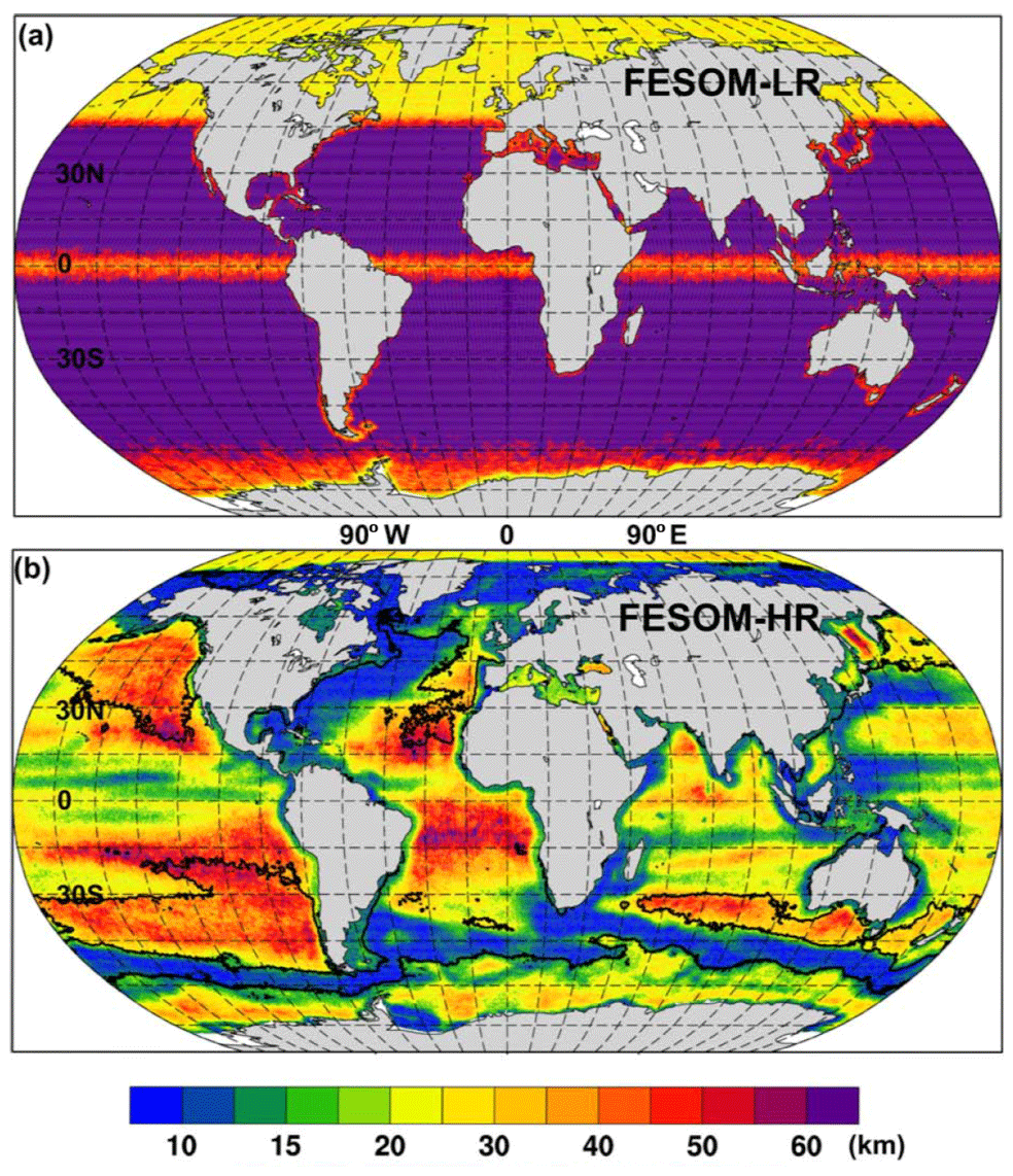
Figure 1Horizontal resolution (km) of the two FESOM grids: (a) low resolution and (b) high resolution.
For the low-resolution configuration, AWI-FESOM uses a nominal 1∘ bulk horizontal resolution, which has been used in previous CORE-II simulations (e.g., Wang et al., 2016a, b), with the North Atlantic subpolar gyre region and Arctic Ocean set to 25 km (see Fig. 1a) and a nearly equatorial resolution of .
For the high-resolution configuration, AWI-FESOM uses the grid introduced by Sein et al. (2016). As the variability of sea surface height (SSH) can manifest the variability of mesoscale eddies, the horizontal resolution is scaled with the strength of the observed SSH variability on this grid. In particular, the resolution is about 10 km along the western boundary currents, the Antarctic Circumpolar Current, and the Agulhas Current region (Fig. 1b). Before generating this grid, the field of SSH variance is smoothed spatially to make sure that the main currents are within high-resolution regions even if their positions change to some extent. The resolution is also increased along the coast and where the observed sea ice concentration variability is high. This multi-resolution grid has about 1.3 million surface grid points, similar to the size of a uniform mesh. In both setups, 46 z levels are used, with 10 m spacing in the upper 100 m. This is slightly less than the 50 levels recommended by Stewart et al. (2017) to resolve the first baroclinic mode in a z-coordinate model.
2.4 IAP-LICOM
IAP-LICOM is a global configuration of the LASG/IAP Climate system Ocean Model (LICOM) (Zhang and Liang, 1989; Liu et al., 2004, 2012; Yu et al., 2018; Lin et al., 2020) developed by the Institute of Atmospheric Physics (IAP) from the Laboratory of Atmospheric Sciences and Geophysical Fluid Dynamics (LASG) of the Chinese Academy of Sciences (CAS). LICOM is the ocean component of the Flexible Global Ocean–Atmosphere–Land System model (FGOALS; e.g., Li et al., 2013; Bao et al., 2013) and of the CAS Earth System Model (CAS-ESM; Minghua Zhang, personal communication, 2019). Version 3 of LICOM (LICOM3) is coupled to CICE4 through the NCAR flux coupler 7 (Craig et al., 2012; Lin et al., 2016). The surface salinity is restored to the monthly PHC3.0 climatology over the entire domain with a salinity piston velocity of 50 m per 4 years (50 m per 30 d for the sea ice regions). However, there is no freshwater flux normalization. The full ocean surface velocity is used in the calculation of wind stress (relative wind stress). The vertical viscosity and diffusion coefficients in the mixed layer are computed by the scheme of Canuto et al. (2001, 2002) with background values of m2 s−1 and an upper limit of m2 s−1. The tidal mixing scheme of St. Laurent et al. (2002) was recently implemented in LICOM3 by Yu et al. (2017). The initial conditions are derived from PHC3.0 for the low-resolution configuration and from the Mercator Ocean reanalysis for the high-resolution configuration.
For the low-resolution configuration, IAP-LICOM uses a Murray (1996) tripolar Arakawa B grid with two north “poles” at 65∘ N, 65∘ E and 65∘ N, 115∘ W with a resolution of approximately 1∘ in both the zonal and meridional directions (360×218 grid points). The vertical grid uses the η coordinate (Mesinger and Janjic, 1985) with 30 levels. The horizontal viscosity consists of a Laplacian with a coefficient of 5400 m2 s−1. The mesoscale eddies are parameterized using the isopycnal tracer diffusion scheme of Redi (1982) and the eddy-induced tracer transport scheme of Gent and McWilliams (1990), with tapering factors as in Large et al. (1997) and the buoyancy-frequency-related (N2) thickness diffusivity of Ferreira et al. (2005).
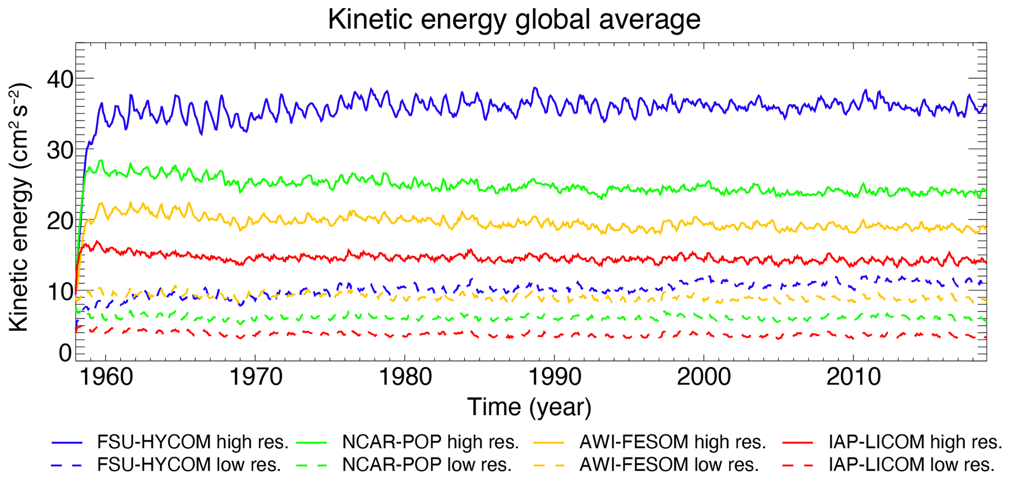
Figure 2Time evolution of the domain-averaged kinetic energy (10−4 m2 s−2) for all experiments.
For the high-resolution configuration (Li et al., 2020), IAP-LICOM uses the same Murray (1996) tripolar grid as in the low-resolution version, but with two north “poles” at 55∘ N, 95∘ E and 55∘ N, 85∘ W and with a resolution of (11 km zonally and varying from 11 km at the Equator to 8 km in midlatitudes – 3600×2302 grid points). There are 55 levels in the vertical, which is just above the minimum recommended by Stewart et al. (2017) to resolve the first baroclinic mode. The additional 25 levels from the low-resolution configuration increase resolution in the deep ocean and improve the simulation of deep circulation and Atlantic meridional overturning circulation (AMOC) transport. The horizontal viscosity consists of a biharmonic operator with a coefficient of m4 s−1. The Gent and McWilliams (1990) scheme is turned off and the tracers use a biharmonic isopycnal diffusivity with a coefficient of m4 s−1. It important to note that only the thermodynamic part of CICE4 (no dynamics) was used in the high-resolution IAP-LICOM.
3.1 Mean kinetic energy
Figure 2 shows the evolution of the domain-averaged mean kinetic energy for all experiments (solid lines for the high-resolution experiments, dashed lines for low-resolution experiments) from 1958 to 2018. The evolution is very similar between different models; all exhibit a quick spin-up of the kinetic energy in the first 5 years, which levels off for the rest of the integration. Not surprisingly, the total kinetic energy is significantly higher for the high-resolution experiments than the low-resolution experiments. For the high-resolution configurations, the FSU-HYCOM has the highest kinetic energy, with a globally averaged value of m2 s−2, and the IAP-LICOM has the lowest kinetic energy, with a globally averaged value of m2 s−2 in the high-resolution configuration. For comparison, a previous high-resolution global simulation, performed with an older version of POP by Maltrud and McClean (2005) using daily NCEP/NCAR reanalysis forcing and absolute winds in wind stress calculations, has a global averaged kinetic energy at 25– m2 s−2 (see their Fig. 1). The higher kinetic energy in FSU-HYCOM can be partially explained by the wind stress formulation, which does not take into account the ocean current velocities (absolute winds), while the other three models do (relative winds). The latter has an “eddy-killing” effect that can reduce the total kinetic energy by as much as 30 % (see Renault et al., 2020, for a review). This is roughly the difference that is seen between FSU-HYCOM and NCAR-POP, and POP with absolute winds in the wind stress (Maltrud and McClean, 2005) has a level of kinetic energy that is close to FSU-HYCOM. But even with the highest resolution used here (∼ 0.1∘), the total kinetic energy remains significantly lower that what can be inferred from observations and higher-resolution models (closer to m2 s−2; Chassignet and Xu, 2017). The increase in total kinetic energy from the low- to the high-resolution configuration is approximately a factor of 4 for all models, except for AWI-FESOM (factor of 2 only). This is probably because the high-resolution AWI-FESOM has a variable grid spacing (Fig. 1b) and does not resolve the Rossby radius of deformation everywhere. The level of total kinetic energy is substantially lower in IAP-LICOM, most likely because of the two-step shape preservation advection scheme used in the momentum equations and higher diffusivity (Table 1).
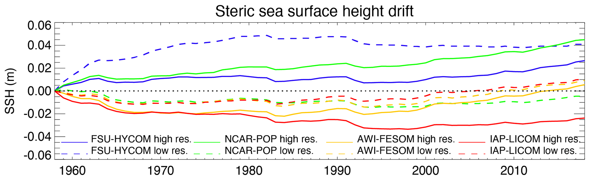
Figure 3Time evolution from the initial conditions of the global steric sea surface height change for all experiments.
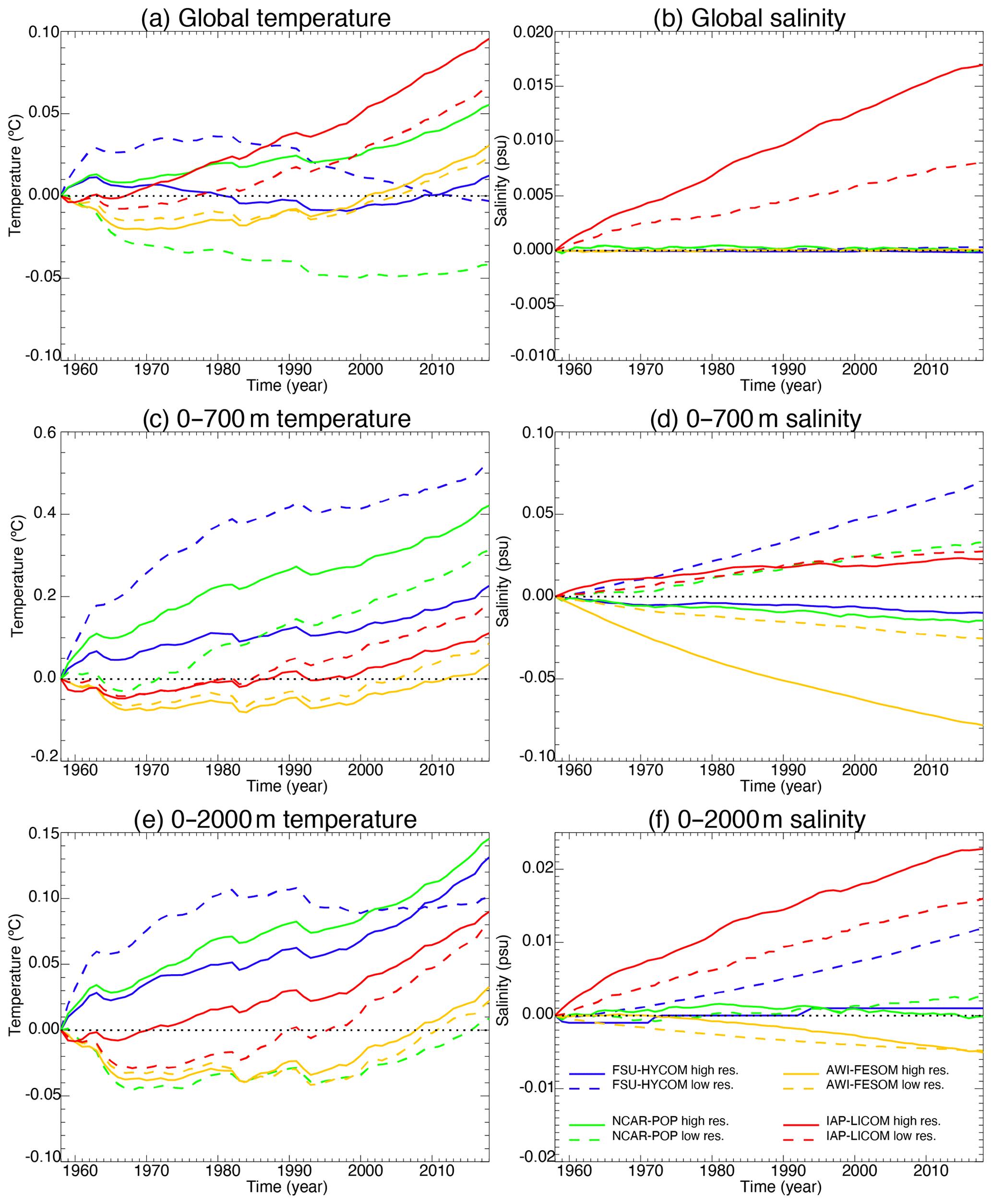
Figure 4Time evolution of global temperature (∘C) and salinity (psu) change (relative to initial conditions) for all experiments (depth-integrated, upper 700 m, upper 2000 m).
3.2 Global mean sea level, temperature, and salinity
As stated by Griffies et al. (2014), “[t]he CORE [and OMIP] protocols (Griffies et al., 2009, 2016; Danabasoglu et al., 2014) introduce a negligible change to the liquid ocean mass (non-Boussinesq) or volume (Boussinesq), and the salt should remain nearly constant (except for relatively small exchanges with the sea ice)”. Changes to the simulated global mean sea level should arise only because of thermosteric effects (i.e., changes in ocean heat content and redistribution of heat) in simulations that preserve salt content (i.e., that have zero net surface freshwater flux). In most models, the global sea level time evolution (Fig. 3) is dominated by changes in the global mean ocean temperature (Fig. 4a). IAP-LICOM is the exception, in which the global sea level shows a downward trend until ∼ 1990 and then slowly rises. This is due to an increase in global mean salinity (Fig. 4b), which dominates the global sea level changes despite a large increase in global volume mean temperature (Fig. 4a). This increase is explained by the lack of surface-restoring salt flux normalization in IAP-LICOM (see Sect. 2.4). For details on the salt flux normalization used in the other models, the reader is referred to Appendix B.3 of Griffies et al. (2009) and Appendix C in Danabasoglu et al. (2014), which describe the techniques used to ensure that there is no net salt added to or removed from the ocean–sea ice system (Griffies et al., 2014). One can also note that most models show an increase in global temperature and sea surface height after 1980–1990, associated with rising air temperature.
An increase in the horizontal resolution does not necessarily imply a reduction in temperature and salinity drift, and no coherent picture emerges from the comparison. If one focuses on the time evolution of the globally averaged temperature in the upper 700 m (Fig. 4c), there are only small changes for AWI-FESOM and IAP-LICOM, while FSU-HYCOM shows a significant reduction in the drift and NCAR-POP an increase as resolution is increased. For salinity in the upper 700 m (Fig. 4d), the increase in resolution significantly reduces the drift in NCAR-POP and FSU-HYCOM; there are no changes for IAP-LICOM and a significant increase for AWI-FESOM. It is important to note that, while the salt flux restoring may differ among the four models, it remains the same for each model as the resolution is increased. When considering the upper 2000 m (Fig. 4f), there is a significant reduction in the global salinity drift for NCAR-POP and FSU-HYCOM, less so for IAP-LICOM, and no changes for AWI-FESOM. We note that most high-resolution models (FSU-HYCOM being the exception) warm faster over the upper 2000 m and global temperature than their lower-resolution partners, which is not true for the upper 700 m. Figure 5 contains identical data as in Fig. 4, except that, by rebasing anomalies to the final year, it highlights the forced ocean variations of the last few decades of simulation by comparing the modeled global temperature and salinity as well as heat and salt content change to that of the World Ocean Atlas 18 (WOA18). The comparison shows that high resolution improves the fidelity and reduces the spread of forced ocean heat content change (particularly 0–2000 m heat content) over recent decades. Figure 6 shows in more detail the evolution of the global temperature and salinity from the initial conditions as a function of depth. AWI-FESOM shows the smallest changes in temperature throughout the water column but the largest in salinity despite having a salt flux adjustment to ensure that the global salinity remains constant (shown in Fig. 2). There is a significant freshening in the upper 400 m compensated for by a salinification in the deeper ocean. This is more pronounced in the high-resolution experiment. Increasing the resolution significantly improves the drift in both temperature and salinity in FSU-HYCOM but not so much in the other simulations. One could actually argue that the drift is stronger in NCAR-POP with a significant warming in the upper 400 m and freshening in the upper 100 m. While it is beyond the scope of this paper, additional insights could be gained by computing vertical heat and salt budgets as in Griffies et al. (2015) and von Storch et al. (2016). In the next section, we investigate in more detail the evolution of temperature and salinity as a function of depth and time by ocean basin.
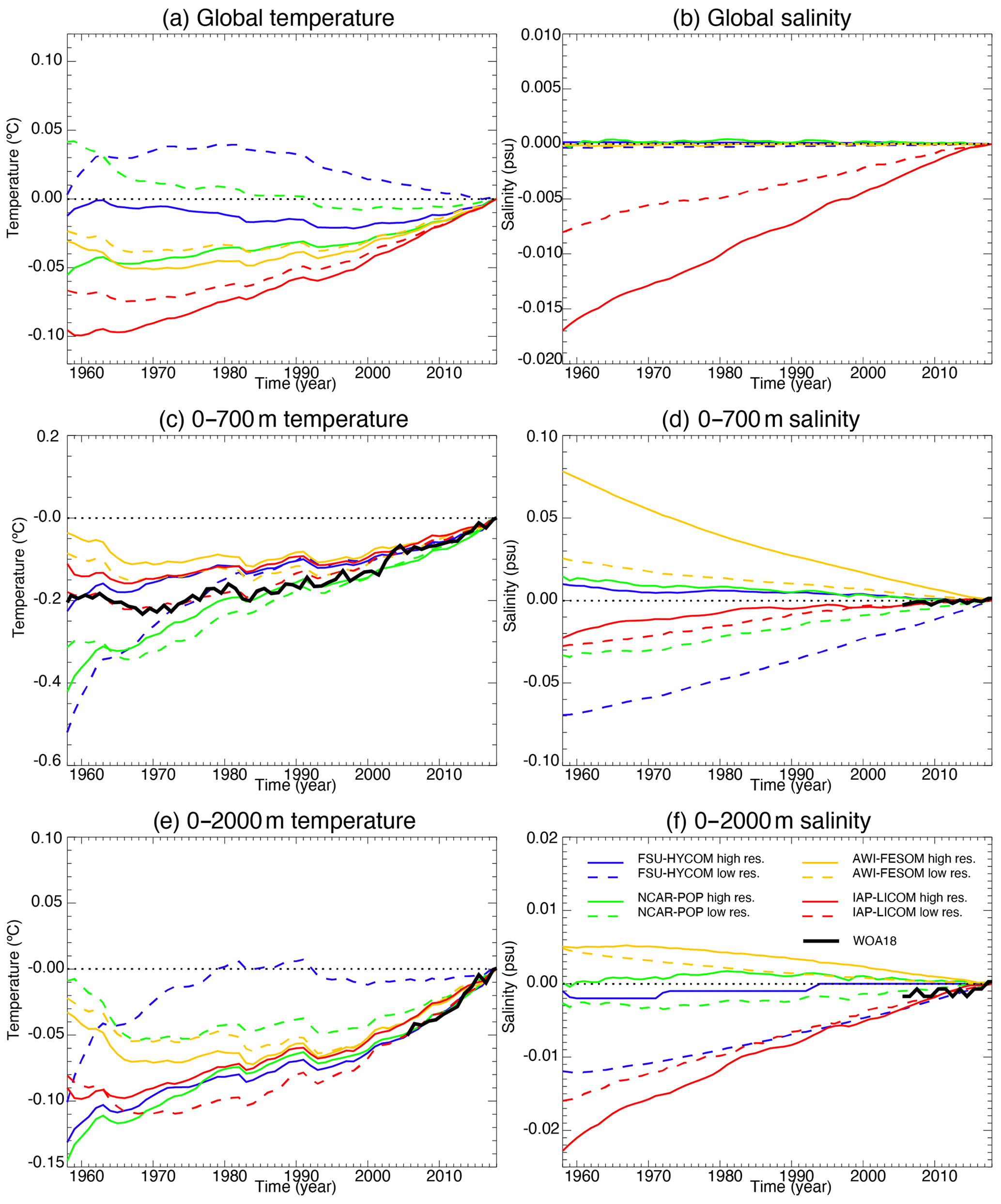
Figure 5Time evolution of global temperature (∘C) and salinity (psu) change (relative to the year 2018) for all experiments and the World Ocean Atlas (WOA18) (depth-integrated, upper 700 m, upper 2000 m).
3.3 Temperature and salinity bias (depth vs. time) by ocean basin
Figures 7, 8, and 9 show the time evolutions of the horizontal mean depth profiles of temperature and salinity for the Atlantic, Pacific, and Indian Ocean, respectively. The color bar is the same in all figures, including Fig. 6 (global), therefore allowing for a qualitative estimate of where the drift is most significant. To a large extent, the time evolution in each of the major ocean basins mimics that of the global but with some significant differences. For the Atlantic Ocean (Fig. 7), there is a surface freshening in the upper 100 to 200 m as resolution is increased in FSU-HYCOM, NCAR-POP, and AWI-FESOM. IAP-LICOM, on the other hand, becomes more saline and warmer in the upper 100 m. The latter is accompanied by a large freshening and cooling below 100 m to approximately 600 m. Overall, the drift is smaller in the Pacific for most models, with a freshening in the upper ocean for all models as resolution is increased. The exception is again IAP-LICOM, which shows a significant increase in salinity in the upper 200 m, and this could be a consequence of the fact that there is no zero normalization of the surface-restoring salt flux. The temperature bias in the Pacific Ocean is similar to that of the global ocean. In the Indian Ocean (Fig. 9), FSU-HYCOM and NCAR-POP exhibit larger biases than AWI-FESOM and IAP-LICOM, but those biases are smaller at the higher resolution.
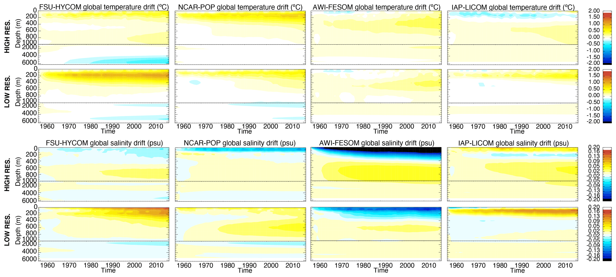
Figure 6Time evolution of global temperature (∘C) and salinity (psu) change (relative to initial conditions) as a function of depth for all experiments.
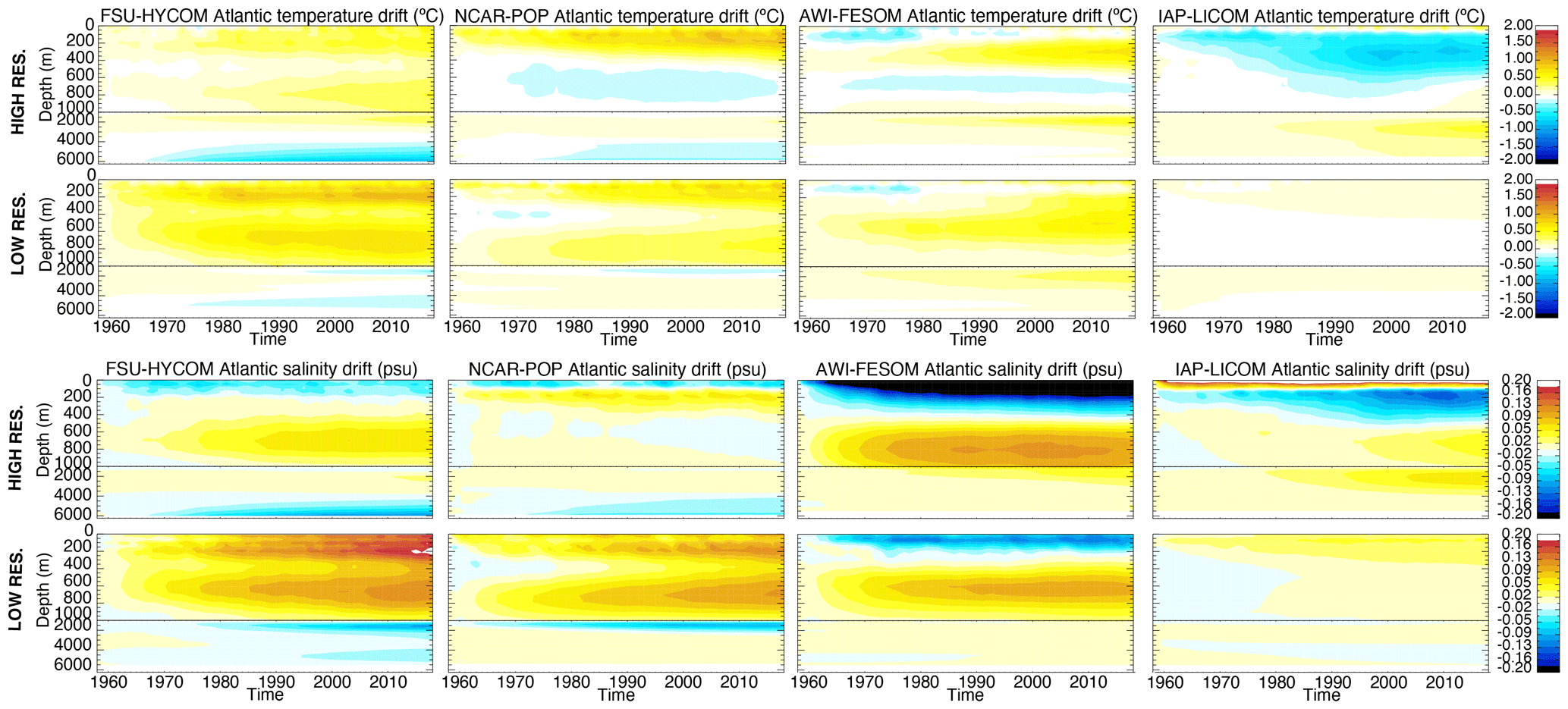
Figure 7Time evolution of Atlantic Ocean temperature (∘C) and salinity (psu) change (relative to initial conditions) as a function of depth for all experiments.
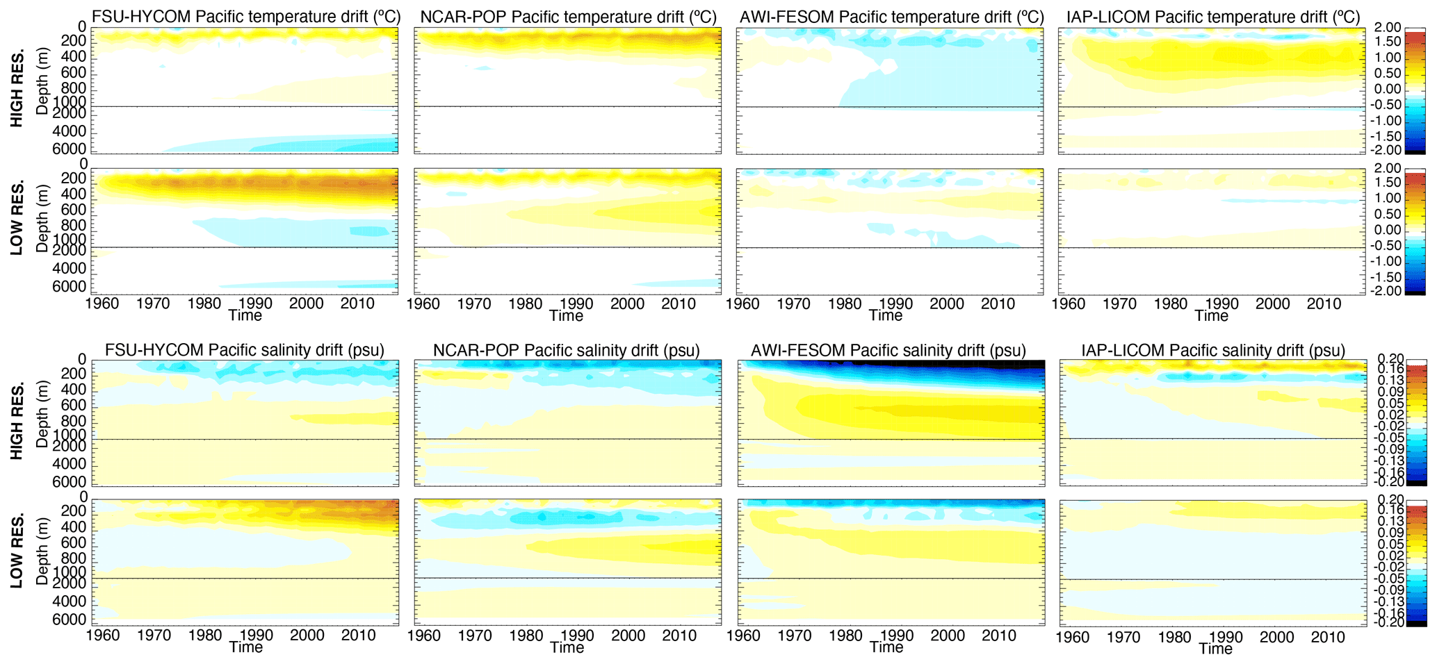
Figure 8Time evolution of Pacific Ocean temperature (∘C) and salinity (psu) change (relative to initial conditions) as a function of depth for all experiments.
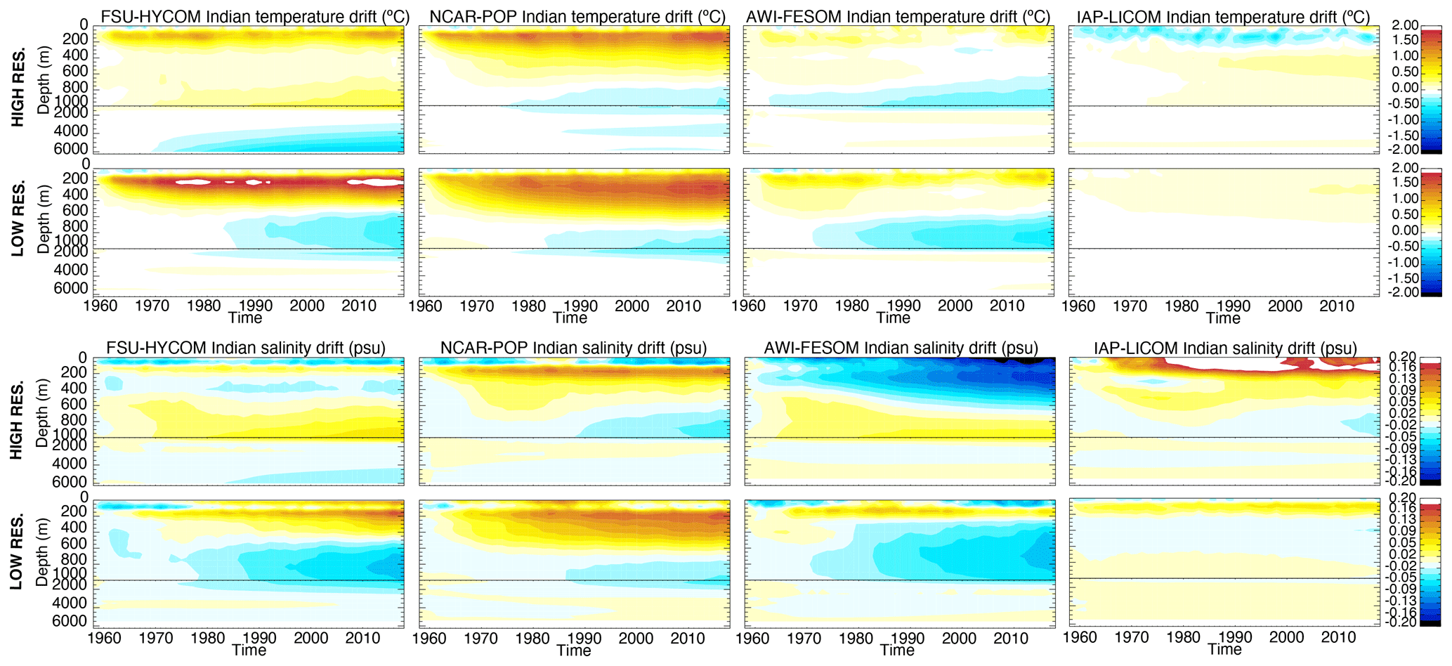
Figure 9Time evolution of Indian Ocean temperature (∘C) and salinity (psu) change (relative to initial conditions) as a function of depth for all experiments.
3.4 Mean temperature and salinity bias
The drift plots from Sect. 3.2 and 3.3 indicate that temperature and salinity bias structures are well-established within the first 2 decades of the spin-up so that time averages computed over the latter decades of the simulations should provide a reasonable estimate of the stationary biases characterizing each model. Figure 10 shows latitude–longitude maps of surface temperature and salinity differences computed over the 1980–2018 time period with respect to WOA18. All models exhibit reductions in sea surface temperature (SST) bias as resolution is increased. The largest bias reductions are seen in the Southern Ocean, in the Agulhas retroflection region, and along the Gulf Stream extension in the North Atlantic. All these changes are presumably primarily related to an improved representation of the pathways of strong surface currents in those regions, which could result not only from differences between resolved and parameterized eddies but also from differences in resolved bathymetry. SST bias in eastern boundary upwelling regions has been shown to be strongly sensitive to atmospheric forcing resolution (Tsujino et al., 2020), somewhat sensitive to the regridding technique used for near-surface winds (Small et al., 2015), and also slightly sensitive to ocean resolution for seasonal means (Kurian et al., 2020). However, Fig. 10 shows a minimal change in annual mean SST bias in the upwelling zones off the west coasts of Namibia, Peru, and North America. In addition to the Gulf Stream, all models exhibit some degree of bias reduction in the Brazil–Malvinas Confluence zone at high resolution, but no such systematic improvement is evident in the Kuroshio–Oyashio extension region. Sea surface salinity bias is generally reduced globally in the high-resolution simulations, with the exception again being AWI-FESOM, which exhibits a more pronounced negative salinity bias in line with the enhanced near-surface salinity drift at high resolution in that model (see Figs. 6–9). The SSS bias in the Arctic results from the differences in salinity between WOA18 and the climatologies used in the salinity restoring (GDEM4, WOA13, or PHC3.0; see Sect. 2 for details).
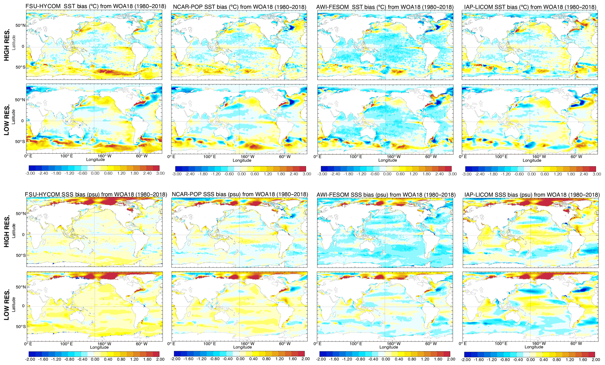
Figure 10Modeled surface temperature (∘C) and salinity (psu) difference from WOA18 over the 1980–2018 time period.
The vertical structure of mean temperature and salinity bias is displayed as zonal averages across the different ocean basins in Figs. 11–13. This reveals that the near-surface global drift toward warming seen in FSU-HYCOM and NCAR-POP is partly related to a degradation of the tropical thermocline in all basins. One hypothesis is that the thermocline bias is related to the representation of vertical eddy heat flux (Griffies et al., 2015), which tends to be stronger and more realistic in high-resolution simulations (see Fig. 5). In FSU-HYCOM, higher resolution improves the situation, while in NCAR-POP, the tropical thermocline temperature bias actually gets worse with resolution. The degradation in thermocline bias in the POP high-resolution version could also be due to missing submesoscale physics, which are parameterized in the low-resolution configuration but absent in the high-resolution configuration. In both FSU-HYCOM and NCAR-POP, and to some extent IAP-LICOM, large extratropical and polar temperature biases associated with intermediate and deep waters decrease with enhanced resolution. In AWI-FESOM, both high- and low-latitude biases get worse. It turns out that the relatively low near-surface temperature drift seen in AWI-FESOM (Figs. 6–9) is related to large, but largely compensating, anomalies of opposite sign at each depth level. Cold–warm anomalies that develop in the tropics and at high latitudes in that model at both resolutions tend to disappear in global or basin-wide means. Such a compensation does not occur for salinity, which is too fresh in the thermocline and too saline in deeper intermediate waters in AWI-FESOM, a characteristic that gets worse as resolution is increased. IAP-LICOM exhibits some large changes in the sign and structure of zonal mean bias as resolution changes, but as with AWI-FESOM, it does not lend strong support to the hypothesis that model temperature and salinity bias can be reduced by increasing model horizontal resolution. As already mentioned, the NCAR-POP model exhibits improved representation of high-latitude intermediate and deep waters, but degraded representation of the tropical thermocline, as resolution is enhanced. FSU-HYCOM is the only model that shows a nearly ubiquitous reduction in temperature and salinity bias in all ocean basins in the high-resolution version; for the other models, greatly enhanced horizontal resolution does not deliver unambiguous bias improvement in all regions. This is a rather unexpected result.
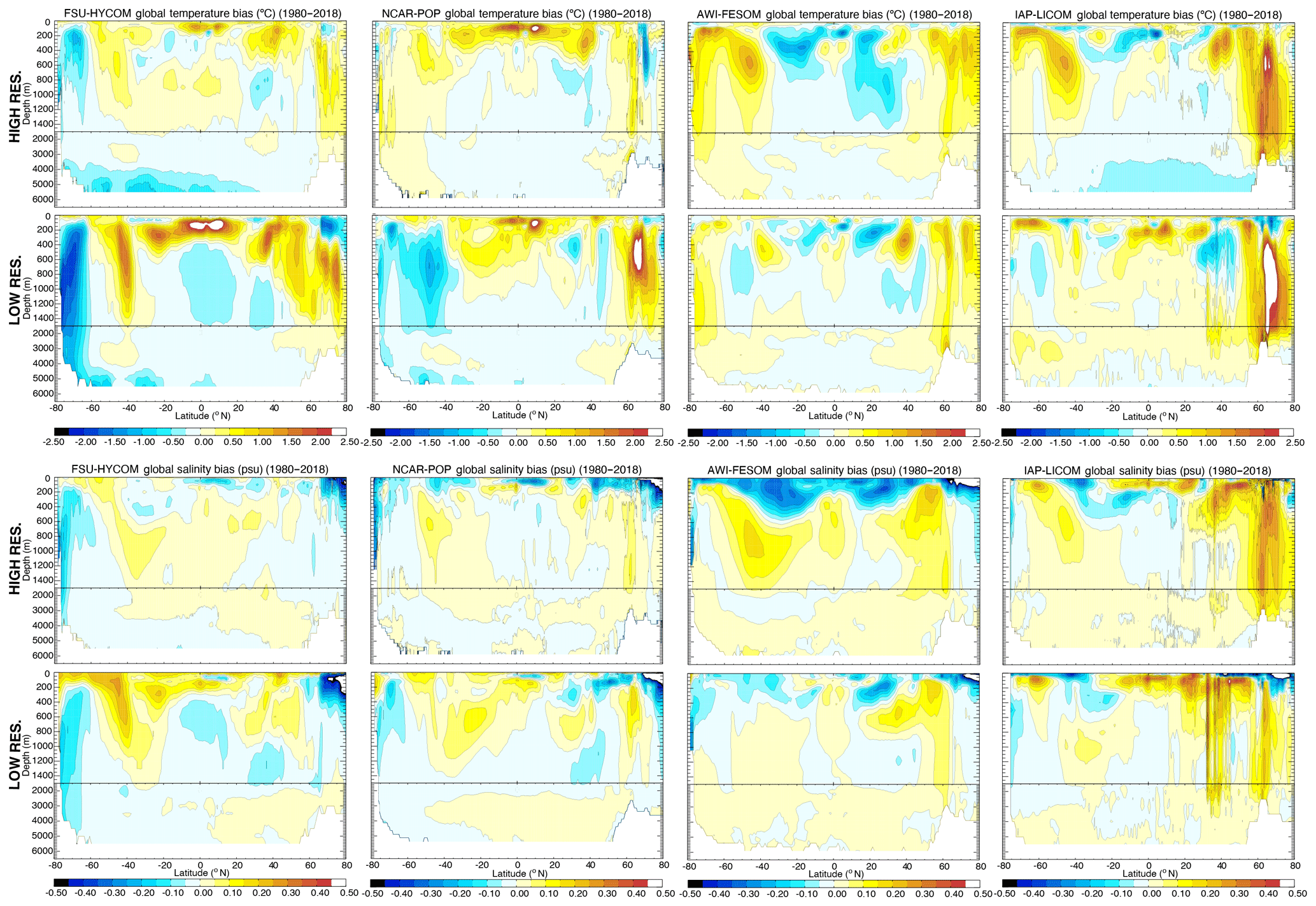
Figure 11Global zonal temperature (∘C) and salinity (psu) difference with the climatology used to initialize the model.
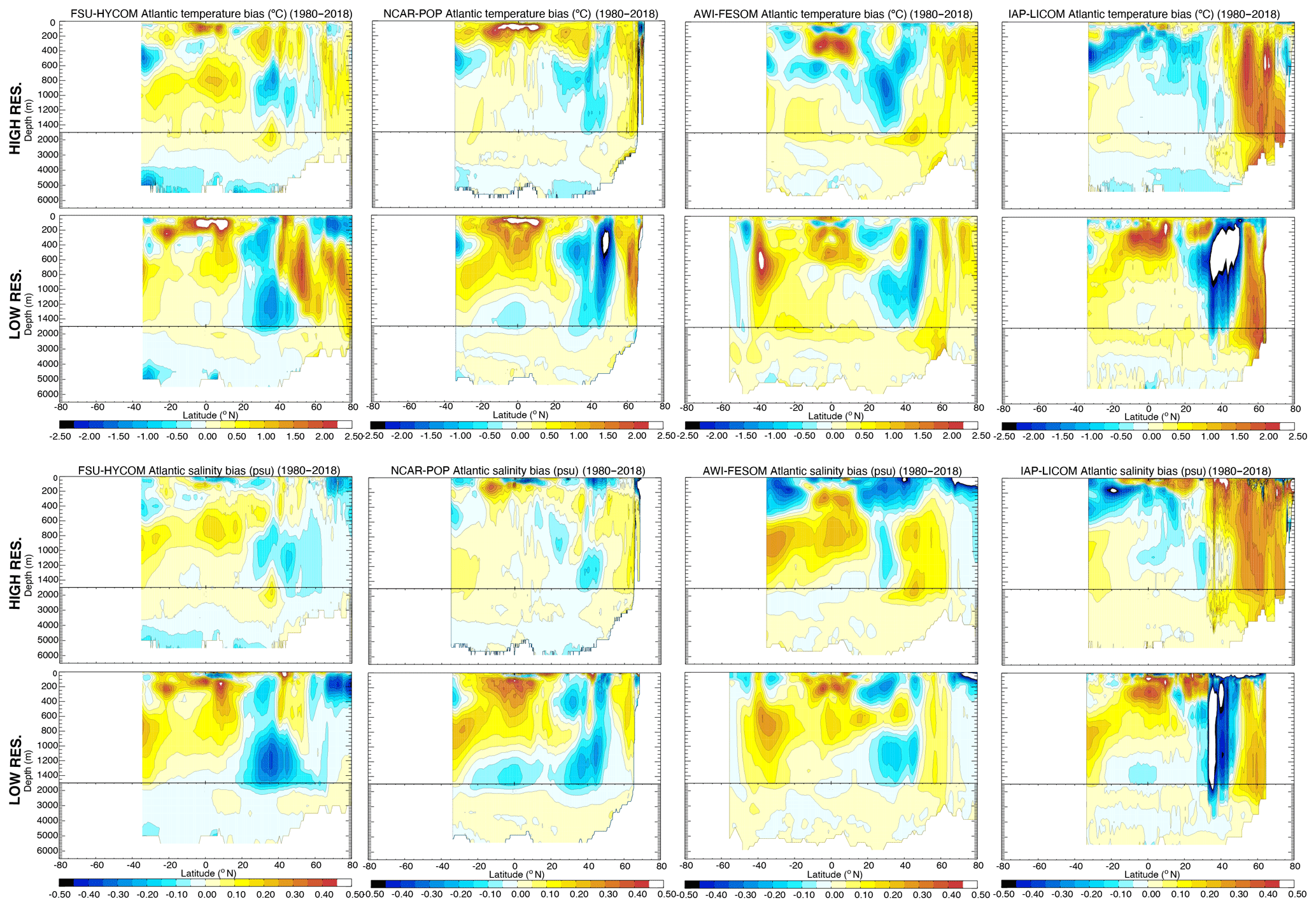
Figure 12Atlantic zonal temperature (∘C) and salinity (psu) difference with the climatology used to initialize the model.
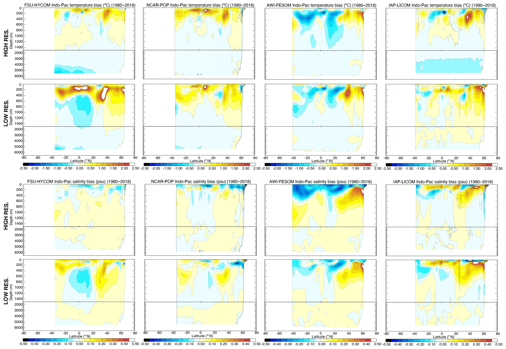
Figure 13Indo-Pacific zonal temperature (∘C) and salinity (psu) difference with the climatology used to initialize the model.
3.5 Northern and Southern Hemisphere sea ice volume and extent
Due to observational constraints, sea ice is often quantified and monitored by passive microwave satellites in terms of sea ice extent (SIE), defined as the sum of all grid areas with 15 % or higher sea ice concentration. Figure 14a–b display the modeled annual mean Northern and Southern Hemisphere sea ice extent for all simulations and include comparisons to the latest observations from the National Snow and Ice Data Center (NSIDC) (Fetterer et al., 2017). Similar to the observations of the 5th and 6th CMIPs (Stroeve et al., 2012; Notz et al., 2020; Shu et al., 2020), the multi-model mean is representative of the passive microwave mean SIE from 1978 to 2018, with large inter-model differences. All models show a clear decline in SIE in the Northern Hemisphere and weaker trends in the Southern Hemisphere. Because observed sea ice extent is highly correlated with near-surface air temperature (e.g., Olonscheck et al., 2019), the consistency of the temporal variability between different simulations and observations suggests that this consistency is driven by a realistic JRA55-do forcing. In general, in both hemispheres, an increase in resolution reduces SIE bias, with the exception of IAP-LICOM.
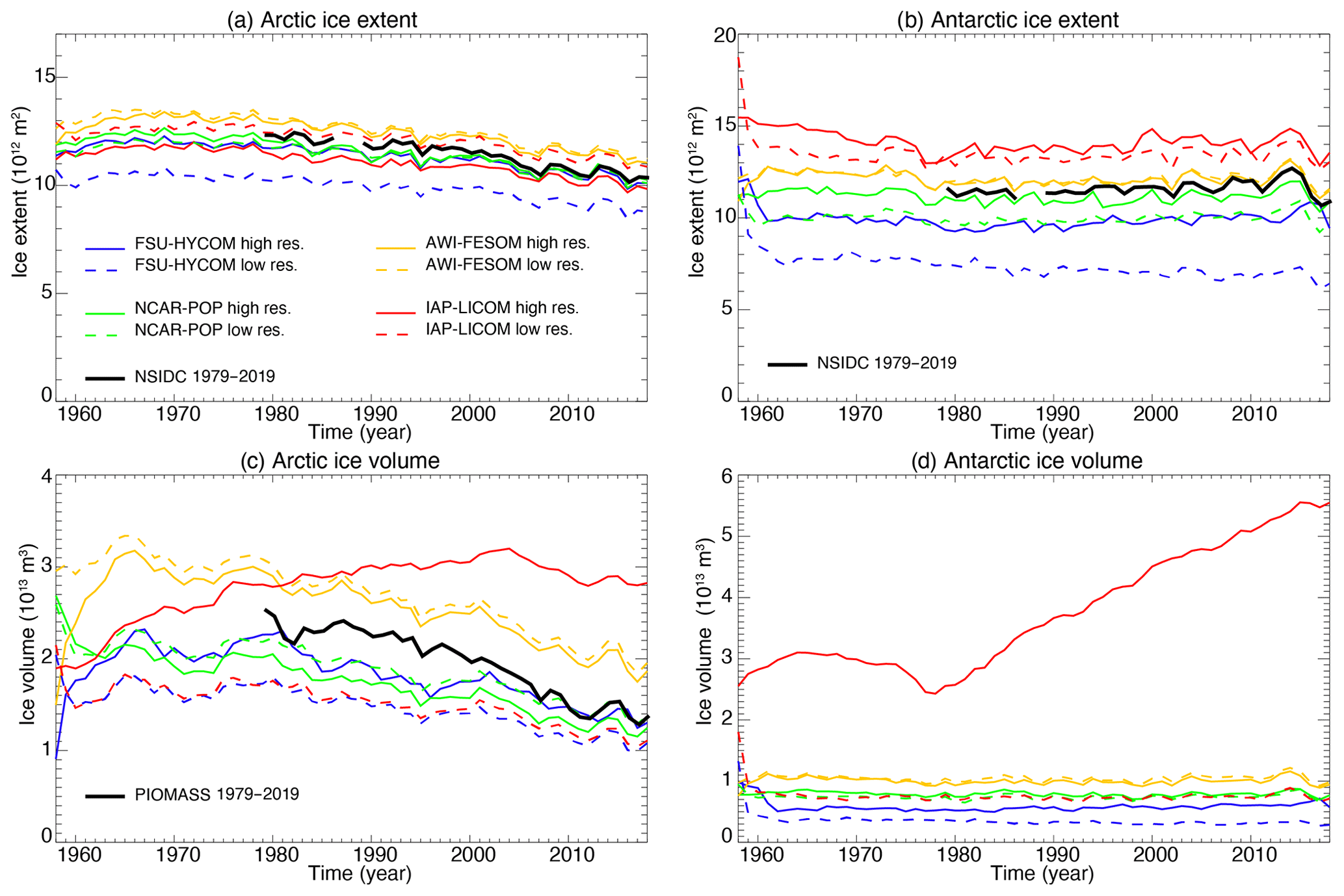
Figure 14Modeled time evolution of annual mean Arctic and Antarctic (a, b) sea ice extent (1012 m2) and (c, d) sea ice volume (1013 m3). The black lines are observations from the National Snow and Ice Data Center (NSIDC) and results the from Pan-Arctic Ice Ocean Modeling and Assimilation System (PIOMAS) (Schweiger et al., 2011).
Sea ice volume (SIV) is a second independent measure of sea ice simulation performance that is representative of sea ice state, determined by the thermodynamical, optical, and dynamical properties of the ice itself, and the sensitivity of modeled SIV to model formulation is insightful for understanding the physical realism of the sea ice schemes. The modeled time evolution of annual mean Northern and Southern Hemisphere SIV is displayed in Fig. 14c and d. Relative to SIE, there is significant inter-model spread in SIV. With the exception of IAP-LICOM, all simulations exhibit a continuous decline in Northern Hemisphere sea ice volume during the satellite era, with trends similar to that of PIOMAS (Schweiger et al., 2011). Changes to SIV also do not appear to be consistent among the models when moving from low to high resolution: it increases for FSU-HYCOM and IAP-LICOM and decreases for NCAR-POP and AWI-FESOM. IAP-LICOM is a clear outlier in both hemispheres, which points to issues in the numerical implementation of its sea ice code at higher resolutions: sea ice thickness on average increases as the resolution is increased despite declining SIE. The IAP-LICOM sea ice model has only thermodynamic processes, and the absence of dynamic sea ice may lead to an excessive accumulation of volume.
3.6 Meridional overturning circulation
The Atlantic meridional overturning circulation (AMOC) is often quantified by a meridional overturning streamfunction with respect to depth, ψz at each latitude, defined as the meridional transport (Sv) across the basin above a constant depth z:
where v is the 4-D meridional velocity, the overbar denotes a time average (here annual mean), and the x integration covers the entire span of the Atlantic basin. The magnitude of the AMOC, or the AMOC transport, is then defined as the maximum of the streamfunction ψz with respect to z, representing the total northward transport above the overturning depth (approximately 1000 m in the Atlantic Ocean). This important measure of the AMOC is quantified and monitored by the RAPID moorings near 26.5∘ N (e.g., Smeed et al., 2018).
The modeled annual mean AMOC transport across 26.5∘ N from 1958 to 2018 is displayed in Fig. 15a, along with the RAPID results (2005–2017) for reference. The vertical distribution of the time mean zonal streamfunction in the Atlantic Ocean is shown later in Fig. 26. For the four models, the high-resolution simulations have a higher AMOC transport than their low-resolution counterparts: the mean AMOC transport in 2004–2018 is 7.8–14.9 Sv in the four low-resolution simulations versus 14.0–19.8 Sv in the four high-resolution simulations (17.2±1.5 Sv as observed by RAPID; e.g., Smeed et al., 2018). However, there is not an obvious difference in the AMOC sensitivity to forcing or in the trend between the low- and high-resolution experiments. The simulated time evolution of the AMOC transports at this latitude depends on the model, its parameterizations, resolution, and the number of spin-up cycles (Danabasoglu et al., 2016). Despite the fact that the simulations were only integrated over one JRA55-do cycle (1958–2018), all four low-resolution models show a similar multi-decadal variability, with a transport decrease from 1958 to the late 1970s, an increase from the late 1970s to late 1990s, and a decrease again thereafter. This multi-decadal variability is also present in the CORE-II simulations (Danabasoglu et al., 2016; Xu et al., 2019). In the high-resolution simulations, FSU-HYCOM, NCAR-POP, and AWI-FESOM exhibit a similar multi-decadal variability (of low transports in the late 1970s and high transports in the early 1990s) as seen in previous basin-scale simulations (e.g., Böning et al., 2006; Xu et al., 2013). The decline in the AMOC transport from the early 1990s to 2000s may be a consequence of the warming and reduced deep convection in the western subpolar North Atlantic that has been documented quite extensively (e.g., Häkkinen and Rhines, 2004; Yashayaev, 2007). The high-resolution AWI-FESOM has a strong AMOC decreasing trend (of 4–5 Sv) initially during the first 20 years and then has a time evolution of the AMOC that is very similar to that of FSU-HYCOM and NCAR-POP. The high-resolution IAP-LICOM shows an increasing AMOC transport from 1958 to the early 1990s (by 10 Sv) and a decrease thereafter (by 5 Sv), which is quite different from the other three models, but it does appear to capture the observed increase over the last few years.
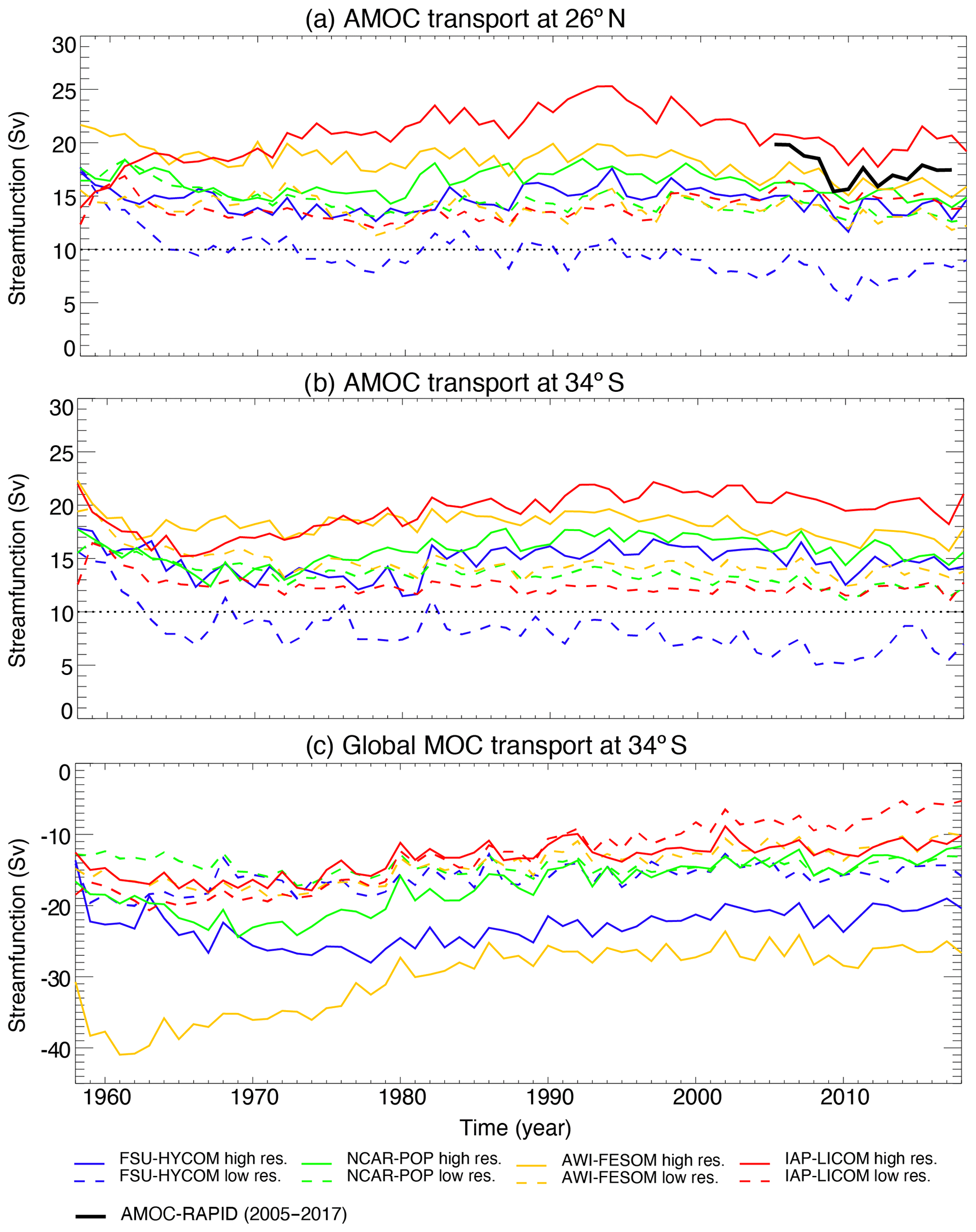
Figure 15Modeled annual mean Atlantic meridional overturning circulation (AMOC) transports at (a) 26.5∘ N and (b) 34∘ S; (c) global meridional overturning circulation (MOC) transports at 34∘ S. The global MOC transport is negative because the northward-flowing Antarctic Bottom Water (AABW) is below the southward return flow (see Lumpkin and Speer (2007) and Talley (2013) for observed values). The solid black line in panel (a) is derived from the RAPID array measurements (Smeed et al., 2018).
AMOC transport in the South Atlantic Ocean has been quantified near 34∘ S using several observational techniques including an expendable bathythermograph (XBT), Argo profiles, and moored current meter arrays in the western and eastern boundaries (Baringer and Garzoli, 2007; Dong et al., 2009, 2014, 2015; Garzoli et al., 2013; Goes et al., 2015; Meinen et al., 2013, 2018); these observations yield a time mean AMOC transport of about 14–20 Sv (see Xu et al., 2020a, for an in-depth discussion of circulation in the South Atlantic Ocean). The modeled temporal evolution of the AMOC transports at this latitude is overall similar to that at 26.5∘ N in the North Atlantic (Fig. 15a, b). The range of the modeled time mean AMOC transport at 34∘ S in the high-resolution simulations, from 14.7 Sv in FSU-HYCOM to 20.1 Sv in IAP-LICOM, is about the same as the observational range mentioned above.
The Antarctic Bottom Water (AABW) cell of the global overturning circulation (Talley, 2013) can be visualized as a streamfunction similar to Eq. (1), except that the zonal integration now spans across the full longitude circle. The transport associated with this cell is defined as the minimum of the streamfunction that is typically found near 3500 m (Lumpkin and Speer, 2007) and is a measure of the northward flow of the near-bottom water (AABW and/or Circumpolar Deep Water, CDW) from the Southern Ocean into the Atlantic, Pacific, and Indian Ocean that eventually upwells and returns southward at a shallower depth. Several observational estimates are provided based on hydrographic sections near 32∘ S, but the uncertainty remains quite high (29±7.6 Sv in Talley, 2013). Figure 15c displays the modeled transport at 34∘ S. The low-resolution simulations show a consistently lower transport, with the mean transport value for 2004–2018 ranging from 7.4 Sv in IAP-LICOM to 15.3 Sv in FSU-HYCOM. The low transport in IAP-LICOM is due to a long-term downward trend in this simulation: from 20 Sv in the early 1960 to 5 Sv in the late 2010s. The other three models, especially FSU-HYCOM, exhibit relatively stable transports in the last 30 years (of the integration). The high-resolution simulations show a much wider range, with time mean transports (2004–2018) ranging from 11.7 Sv in IAP-LICOM to 26.5 Sv in AWI-FESOM. The time evolution of the 34∘ S transports in the high-resolution simulations typically shows an increase in the early stage of the integration followed by a gradual decrease afterward. But the timescale of the increase and decrease periods varies significantly between models. As a result, the transport is relatively stable in IAP-LICOM and AWI-FESOM for the last 30 years of the integration but continues to decrease slowly in NCAR-POP and FSU-HYCOM. Interestingly, despite the large difference in time mean transports, all four high-resolution models exhibit a similar interannual variability at this latitude for the last 30 years of the integration.
3.7 Drake Passage and Indonesian Throughflow transports
The Antarctic Circumpolar Current (ACC) is a strong oceanic current that flows eastward around Antarctica. It connects the Pacific, Atlantic, and Indian Ocean to its north and is the primary means of inter-basin exchange, enabling a truly global overturning circulation (e.g., Gordon, 1986; Schmitz, 1996; Talley, 2013). Accurate knowledge of ACC transport is fundamental to understand its influence on global circulation. Substantial observational efforts have been made toward quantifying ACC transport, especially in the Drake Passage, where the ACC is constricted between the Antarctica and the southern tip of South America. The major observations include (1) the International Southern Ocean Studies (ISOS) program in the late 1970s and early 1980s (Whitworth, 1983; Whitworth and Peterson, 1985), (2) the repeat hydrographic sections along the World Ocean Circulation Experiment (WOCE) line SR1b (e.g., Cunningham et al., 2003), (3) the repeat shipboard acoustic Doppler current profiler (ADCP) surveys that directly measure the current in the top 1000 m of the water column (Firing et al., 2011), (4) the DRAKE program that combines a moored current meter array (2006–2009) and satellite observations (e.g., Koenig et al., 2014), and (5) the cDrake program with a high-resolution bottom current meter mooring array and cPIES observations from 2007 to 2011 (e.g., Chidichimo et al., 2014; Donohue et al., 2016). The time mean, full-column transport estimates range from 134±15 Sv based on ISOS, to 141±2.7 Sv based on DRAKE program, and to 173.3±10.7 Sv based on the cDrake results.
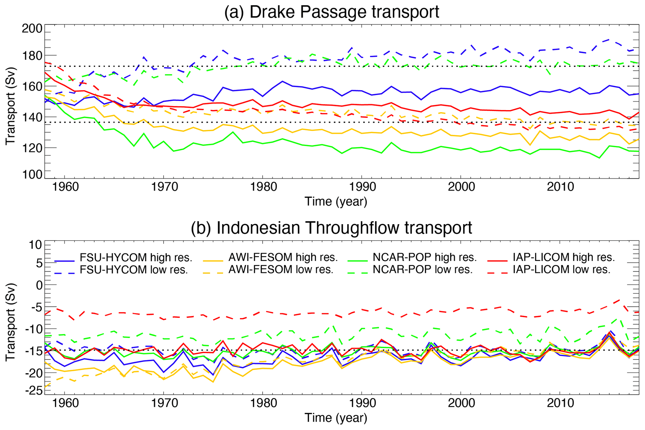
Figure 16Modeled annual mean volume transport of the ACC through the Drake Passage and of the Indonesian Throughflow (ITF) from the Pacific to Indian Ocean. The dotted lines in (a) represent the observational range between the canonical transport value (134 Sv) based on the ISOS program and 173 Sv based on cDrake observations. The dotted line in (b) is the observed ITF transport value (15 Sv) based on INSTANT observations.
The modeled annual mean Drake Passage transport is displayed in Fig. 16a together with the mean observational range (134–173 Sv). The transports in the low-resolution simulations differ from each other: IAP-LICOM and AWI-FESOM show a continuous decrease and FSU-HYCOM shows a continuous increase, whereas NCAR-POP shows an increase in the first 20 years, then levels off for the next 40 years of the integration. It is expected that the low-resolution models will be sensitive to different parameterizations and their ability to simulate eddy saturation (Gent and Danabasoglu, 2011; Munday et al. 2013). As a result, the time mean transport for the last 15 years of these low-resolution simulations is either near the edge or outside the above observational range: 132, 135, 173, and 190 Sv, respectively, for IAP-LICOM, AWI-FESOM, NCAR-POP, and FSU-HYCOM. The evolution of Drake Passage transport is slightly more similar in high-resolution simulations (compared to the low-resolution counterparts). Even at high resolution, mean ACC transport is sensitive to subgrid schemes (Pearson et al., 2017). Three models show a fast decrease in the first 10–15 years and then a very small decrease thereafter, except that FSU-HYCOM shows a small increase in the first 20 years and then levels off thereafter. The high-resolution models exhibit a higher interannual variability correlation than the low-resolution models. The ACC transports in NCAR-POP and AWI-FESOM of 120 and 130 Sv, respectively, are lower than the latest best mean transport estimate (Xu et al., 2020b) but still within the uncertainty range, while the transports in IAP-LICOM and FSU-HYCOM of 145 and 157 Sv, respectively, are within the mean observational range.
The long-term trend in modeled ACC transport merits some further discussions. Observations indicate that, as shown by a higher Southern Annular Mode index, the westerly winds in the Southern Ocean have been intensified since the 1970s. This increase in westerly winds is also present in the JRA55-do forcing, yet none of the high-resolution simulations exhibit a long-term upward trend (three models even have a slightly weakening trend). The ACC transport time series from the DRAKE program (Koenig et al., 2014) and from the WOCE line SR1b also show a stable ACC transport from early 1990s. Given that the ACC is wind-driven, a lack of dependence for ACC transport on zonal wind at a long-term timescale may at first be surprising, but it has also been shown that the strengthening of winds does generate more eddy activity along the path of the ACC, without necessarily changing its total transport (e.g., Hallberg and Gnanadesikan, 2006; Morrison and Hogg, 2013; Munday et al., 2013; Farneti et al., 2015). Following this argument, one may expect to see an increasing ACC transport in low-resolution, non-eddying simulations as long as the coefficient used in the eddy parameterization (i.e., GM) remains constant (Gent and Danabasoglu, 2011). Only FSU-HYCOM shows a long-term increase in the ACC transport, and two models (IAP-LICOM and AWI-FESOM) even show a long-term decrease. This may be a consequence of the eddy parameterization choice made by the different models, assuming that the ACC is quasi-equilibrated and that changes are not related to buoyancy changes in the Southern Ocean (e.g., rate of bottom water formation). There is, however, an initial condition transient in the buoyancy gradients across the ACC (Fig. 15c), and the MOC across the ACC is equilibrating for a significant fraction of the integration time: one cannot rule out the possibility that the ACC changes result from buoyancy drifts. All models have weaker Drake Passage transports at higher resolution, except for IAP-LICOM.
The Indonesian Throughflow (ITF) connects the tropical Pacific and Indian Ocean and provides a pathway for inter-basin exchange of heat and fresh water. Tropical Pacific and Indian Ocean water masses can go through the ITF and contribute to the upper AMOC limb in the South Atlantic Ocean as part of the global MOC via the Agulhas Current (e.g., Gordon, 1986; Schmitz, 1996; Talley, 2013). A good overview of the Indonesian Sea oceanography and the ITF observations can be found in Gordon (2005) and Gordon et al. (2010). The 3-year mean total ITF transport measured by the International Nusantara Stratification and Transport (INSTANT) program in 2004–2006 is 15±2.5 Sv (Sprintall et al., 2009; Gordon et al., 2010), about 30 % greater than the values of nonsimultaneous measurements made prior to 2000. ITF transport variability exhibits a close relationship to the phase of the El Niño–Southern Oscillation (Meyers, 1996).
The modeled annual mean ITF transport is displayed in Fig. 16b. The low-resolution simulations exhibit a wide range of ITF transports, ranging from about 5 Sv in the IAP model, to 11 Sv in the NCAR-POP model, and to 15 Sv in FSU-HYCOM and AWI-FESOM (30-year mean). ITF transports exhibit a gradual decrease in AWI-FESOM but are relatively stable in the other three models. In the high-resolution simulations, however, the models yielded a quite similar ITF transport, especially in the second half of the integration. All four models represented a similar mean transport of 15 Sv that is close to observations and all show a very similar variability. While large-scale forcing mechanisms are thought to set the basic level of ITF transport (Godfrey, 1989), the difference between the low-resolution and high-resolution simulations is likely impacted by the model ability to represent the small-scale bathymetry feature of the Indonesian Seas (Jochum et al., 2009); after all, the ITF enters the Indian Ocean through a number of narrow straits that are hard to represent in the low-resolution models. IAP-LICOM and NCAR-POP have low ITF transports at low resolution and appear to have stronger sensitivity to model resolution.
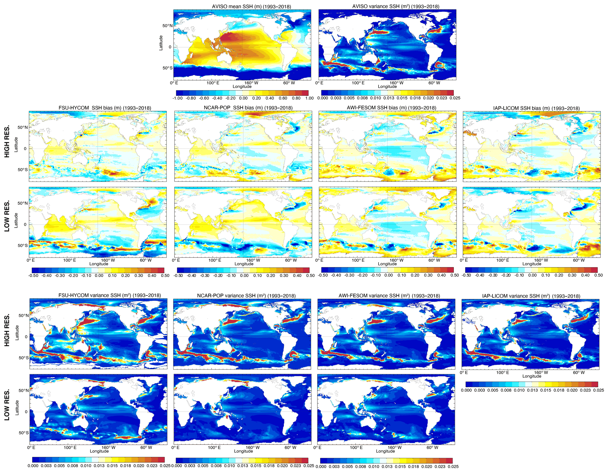
Figure 17Top panels: mean 1993–2018 SSH and variance AVISO. Middle panels: difference between the mean modeled SSH and AVISO SSH. Bottom panels: modeled variance derived from 5 d average outputs. The low-resolution IAP-LICOM SSH variance was not provided.
4.1 Sea surface height (SSH) and eddy kinetic energy (EKE)
The impact on the circulation of increasing the horizontal resolution is twofold. First, the solution becomes more nonlinear and allows for a better representation of western boundary currents. Second, the first Rossby radius of deformation is resolved over most of the globe (Hallberg, 2013) and eddies are formed through barotropic and baroclinic instabilities, although higher vertical modes including submesoscale eddies are not often resolved (nor are they resolved by altimetry, i.e., AVISO) (see Stewart et al., 2017). Figure 17 displays the mean sea surface height bias with respect to AVISO and its 5 d variance over the 1993–2018 period. Overall, the large-scale patterns are well-represented globally, and one can clearly see the improved representation of the western boundary currents as resolution is increased (Gulf Stream and Kuroshio). In the North Atlantic, most coarse-resolution models to date have the tendency to exhibit an overshooting Gulf Stream and a poor representation of the North Atlantic Current (NAC) at the Northwest Corner. This is the case for three out of the four models. Instead of flowing northeastward along the continental rise past the Flemish Cap and continuing northwestward as in the observations (Rossby, 1996), the North Atlantic Current is strongly zonal in NCAR-POP, AWI-FESOM, and IAP-LICOM and does not turn northeastward at the Flemish Cap. This has been a long-standing issue for many ocean components of the CMIP climate models, and it does not necessarily improve as the computational mesh is refined. Increasing the horizontal resolution did improve the Gulf Stream separation (see Chassignet and Marshall, 2008, and Chassignet and Xu, 2017, for a review) in all models but not necessarily the representation of the Northwest Corner circulation (Fig. 17; see Fig. 1 in Chassignet et al., 2020a, for details). FSU-HYCOM is the only model that has a good representation of the Northwest Corner in both the low- and high-resolution experiments. Since all the models use the same atmospheric forcing dataset, the difference is solely due to the numerical and physical choices made by each modeling group.
As expected, there is a significant increase in the SSH variance as resolution is increased, and the eddying solution SSH variance maps are much closer to the observations (top panels) than their low-resolution counterparts. In the high-resolution experiments (∼ 0.1∘), the variability is, however, still lower than observed, especially in the gyre interiors and in the experiments that use relative winds (NCAR-POP, AWI-FESOM, and IAP-LICOM). This underestimation is thus partly a consequence of the well-known eddy-killing effect, which results from taking into account the shear between atmospheric wind and ocean current when computing the wind stress and which can reduce the kinetic energy by as much as 30 % (see discussion in Sect. 3.1). However, the use of absolute wind in FSU-HYCOM is not sufficient to raise the level of surface variability to that of the observations, and Chassignet and Xu (2017) argue that one actually needs to significantly increase the resolution (∼ 0.01∘) in order to resolve the submesoscale instabilities that can energize the mesoscale (Callies et al., 2016) and therefore enhance eddy kinetic energy comparable to the mesoscale AVISO observations. It is more physical to take into account the vertical shear between atmospheric winds and ocean currents when computing the wind stress (see Renault et al., 2020, for a review) as it allows for a better representation of western boundary current systems (Ma et al., 2016), especially the Agulhas Current retroflection and associated eddies (Renault et al., 2017). In FSU-HYCOM, which uses absolute wind, the Agulhas eddies are too regular and follow the same pathway. The use of relative winds not only increases the eddy decay, but also impacts the location of the Agulhas retroflection and where the eddies are formed. The three simulations with relative winds have a better representation of the Agulhas eddy pathways.
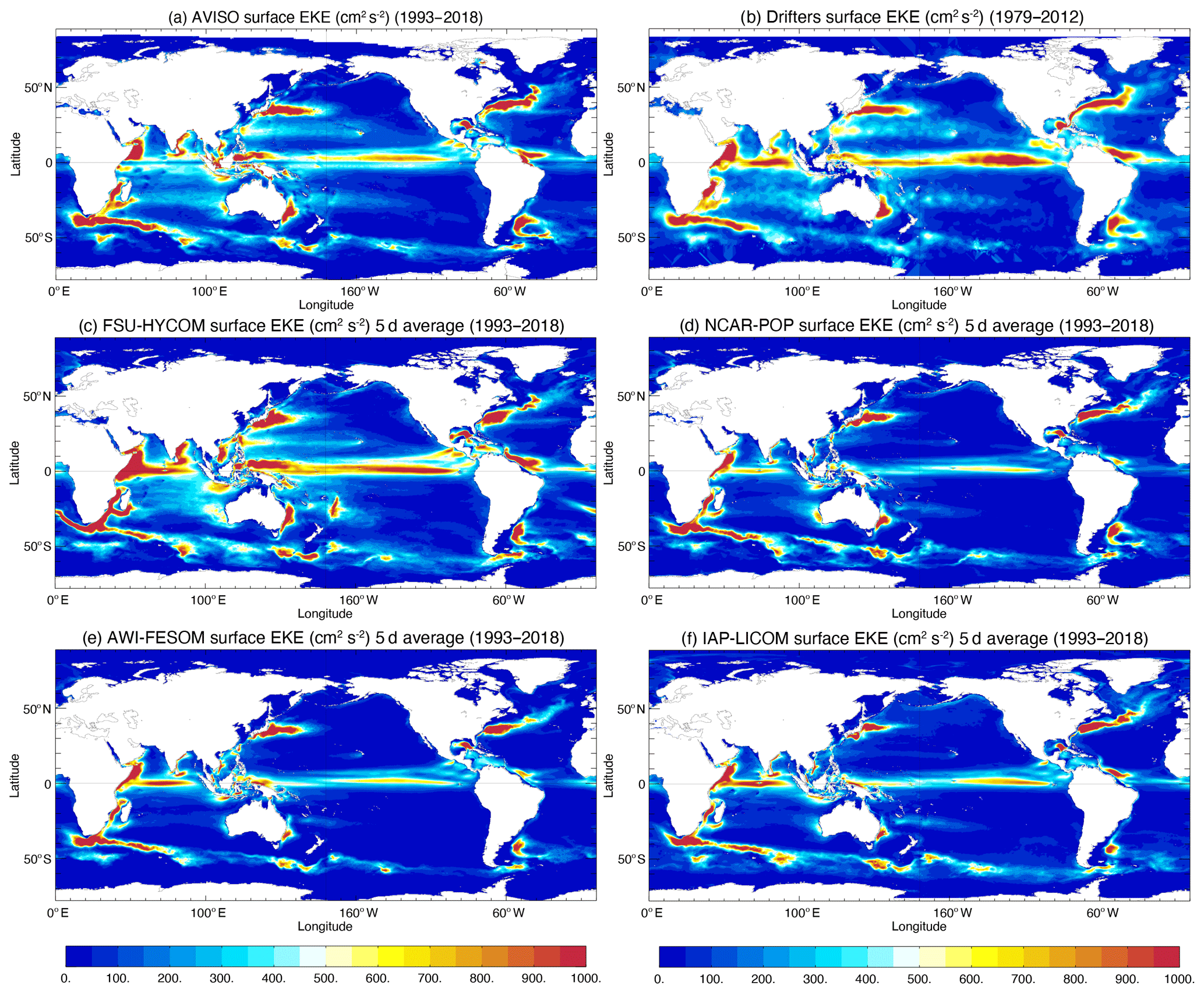
Figure 18Surface EKE from (a) AVISO and (b) drifter observations. Modeled surface EKE calculated from 5 d average fields for the high-resolution (c) FSU-HYCOM, (d) NCAR-POP, (e) AWI-FESOM, and (f) IAP-LICOM.
The eddy kinetic energy maps for the high-resolution simulations are displayed in Figs. 18–21 for the surface, at 700 m, and at 1000 m. Observed surface EKE maps are either derived from altimetry (Fig. 18a) or drifters (Fig. 18b). Because of the irregular sampling, this necessarily implies some type of smoothing in space and time. In the case of the AVISO along-track altimetry observations, they are optimally interpolated on a 0.25∘ grid, which filters scales less than 150 km (due to track separation and measurement noise and errors) and timescales less than 10 d (repeat cycle of the altimeters). There is a significant reduction in EKE when computing it using 5 or 10 d average outputs (as opposed to online at every time step) as shown in Fig. 19 for FSU-HYCOM and NCAR-POP. In addition to a significant EKE reduction in the most active regions, the time averaging removes much of the small-scale variability associated with inertial motions and ageostrophic effects. There is not a big difference between the 5 d and the 10 d maps, and for the rest of this section we will use 5 d average model outputs when comparing the EKE to observations. Overall, as for the SSH variability, the EKE is larger in FSU-HYCOM because absolute winds are used to force the models. As already discussed, the use of relative winds does improve the pathway for the Agulhas Current eddies, but in Fig. 18 there is also a significant reduction of EKE in the ACC, and it also suppresses variability in many areas. This is especially true for the Indian Ocean, in the tropics, and west of the Hawaiian Islands.
Most model–observation comparisons usually focus on the surface fields because of very sparse spatiotemporal sampling at depth (see, for example, the EKE derived at 700 m from several years of SOFAR float measurements in the Gulf Stream region, Richardson, 1993, or the EKE distribution from ARGO floats at 1000 m, Ollitrault and Colin de Verdière, 2014). Scott et al. (2010) evaluated the total kinetic energy simulated in eddying ocean models (on the order of 0.1∘ horizontal resolution) relative to moored current records. They found that the models agreed within a factor of 2 above 3500 m of depth and within a factor of 3 below 3500 m of depth. Thoppil et al. (2011) show that the surface and abyssal EKE increases with resolution and that better upper-ocean EKE allows strong eddy-driven abyssal circulation. This also means that, while the EKE at depth in the high-resolution experiments is a significant improvement over the quasi-nonexistent EKE of the low-resolution simulations, it is still significantly less than very limited observations (Richardson, 1993; Ollitrault and Colin de Verdière, 2014). Significantly higher resolution may be necessary in order to obtain a level of EKE close to the observations (see Chassignet and Xu, 2017, for a discussion). When using relative winds at this resolution as in NCAR-POP, AWI-FESOM, or IAP-LICOM, there is very little EKE at depth when compared to FSU-HYCOM forced with absolute winds (Figs. 20 and 21).

Figure 19Comparison of surface EKE calculated from the total integrated kinetic energy, 5 d average fields, and 10 d average fields in the high-resolution FSU-HYCOM and NCAR-POP.
4.2 Sea surface temperature (SST) and sea surface salinity (SSS) deseasonalized variance
Surface temperature and salinity show sensitivities to resolution that are largely consistent with those described above for SSH in terms of both mean state and variability. All models show greatly enhanced SST variance (computed from deseasonalized monthly values spanning 1980–2018) at high resolution in regions of high mesoscale eddy activity, including the Southern Ocean, the Agulhas Current retroflection, the Brazil–Malvinas Confluence region, the Kuroshio and its extension across the North Pacific, and the Gulf Stream and its NAC extension (Fig. 22). A global, satellite-based SST dataset spanning 1982–2018 provides some measure of ground truth for comparison, but the sampling limitations of microwave and infrared measurements of SST restrict the observed estimate to a (1∕4∘) grid that is 2–3 times coarser than the high-resolution model grids considered here (OISST.v2; Reynolds et al., 2007; Banzon et al., 2014).
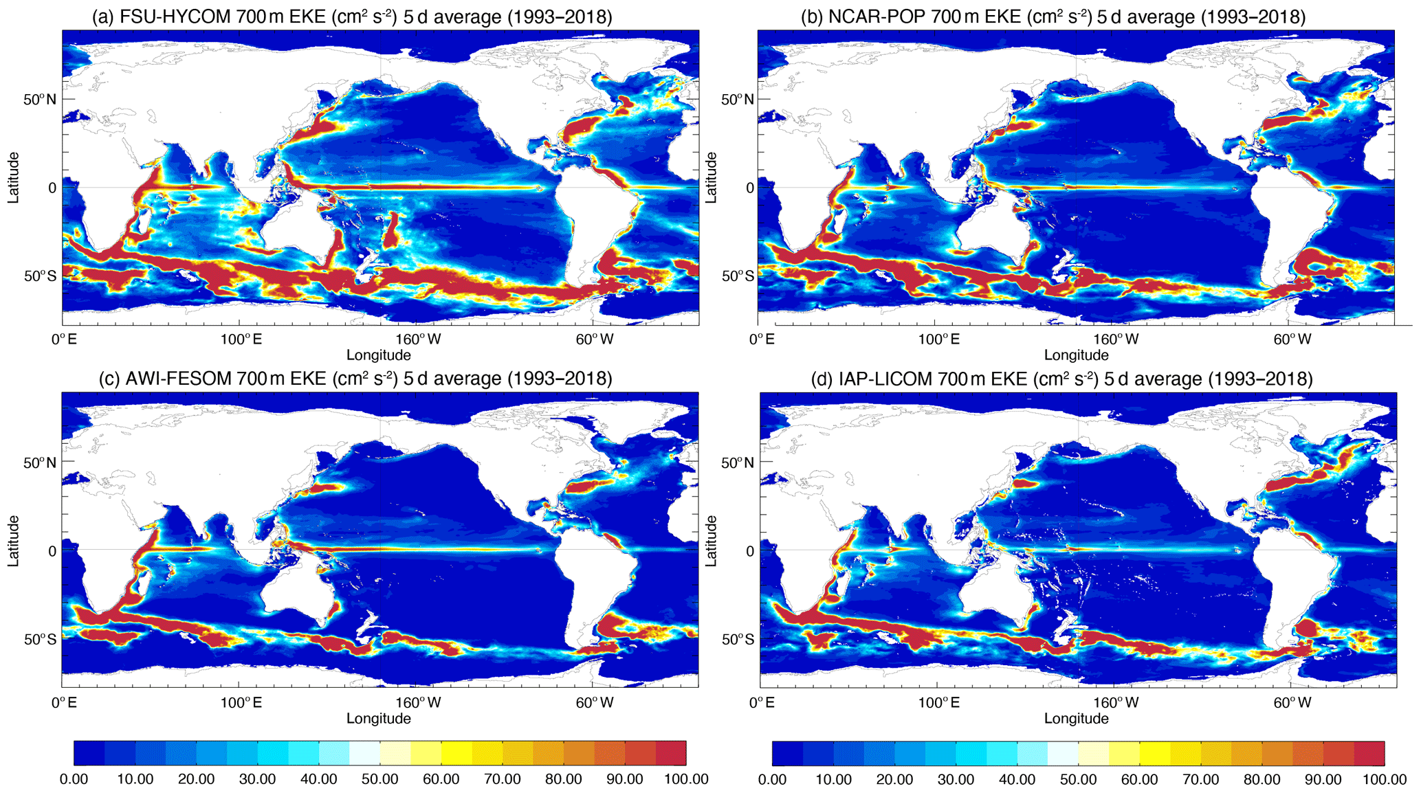
Figure 20EKE at 700 m calculated from 5 d average fields in (a) FSU-HYCOM, (b) NCAR-POP, (c) AWI-FESOM, and (d) IAP-LICOM.

Figure 21EKE at 1000 m calculated from 5 d average fields in (a) FSU-HYCOM, (b) NCAR-POP, (c) AWI-FESOM, and (d) IAP-LICOM.
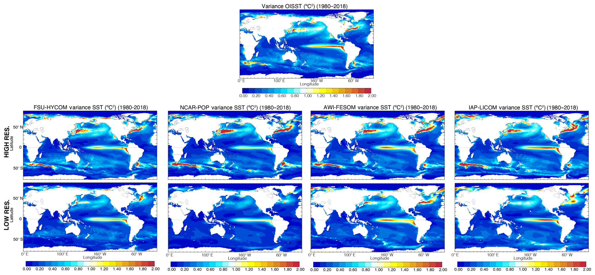
Figure 22Modeled and observed (OISST) deseasonalized SST variance.
As was noted for SSH, the high-resolution FSU-HYCOM simulation generally exhibits the highest SST variance in the midlatitude gyre interiors compared to other models, but it has lower SST variance in strongly eddying regions such as the Agulhas retroflection, Kuroshio, and NAC. Overall, the high-resolution FSU-HYCOM shows the closest match to the observed benchmark. The improved structure of SST variance in the subpolar Atlantic in FSU-HYCOM is related to the improved NAC pathway in that model (discussed above). Compared to OISST.v2, the low-resolution models generally underestimate SST variance, while the high-resolution models tend to overestimate the variance, particularly in the western boundary currents, Southern Ocean, and Agulhas retroflection region. The resolution sensitivity is most dramatic in the NCAR-POP model, whose low-resolution version shows the weakest SST variance of any of the simulations considered here. The overestimation of SST variance has been noted before in eddy-resolving coupled simulations (e.g., Small et al., 2014), but it is not clear whether this discrepancy is attributable to deficiencies in the models or in the observation-based estimates, which cannot fully resolve ocean mesoscale variability. The absence of a dynamic (and ocean mesoscale-resolving) atmosphere in these simulations may partially explain the overly high SST variance insofar as important eddy-damping processes (Ma et al., 2016) are missing in this experimental framework. It is interesting that all high-resolution simulations generate more SST variance in the Kuroshio region than seen in OISST.v2, and yet they all show less variance than observed in the northeast Pacific and along the southeastern branch of the North Pacific gyre (near Hawaii). There is an indication of slightly enhanced ENSO-related tropical Pacific SST variance when going from low to high resolution, but there is not a systematic change in the spatial structure of this variance, which appears to depend mainly on model formulation. The representation of high extratropical SST variance along the eastern boundaries of each of the major ocean basins shows robust improvement with resolution across the different models. The high-resolution versions all show higher (and more realistic) variance in the following locations: the Benguela Current region in the eastern South Atlantic; the coastal region off the west coast of North America and Baja; the Leeuwin Current region off the west coast of Australia; and the Canary Current region off the west coast of North Africa. Improvements in simulated SST variability in these regions are more apparent than improvements in the mean state (Fig. 10). The overall picture of greatly enhanced SST variance at eddying resolution is an important, but not unexpected, result that has significant implications for climate modeling because resolving air–sea interactions at the ocean mesoscale has been shown to result in qualitatively different coupled model behavior (e.g., Bryan et al., 2010; Ma et al., 2016, 2017; Laurindo et al., 2019).
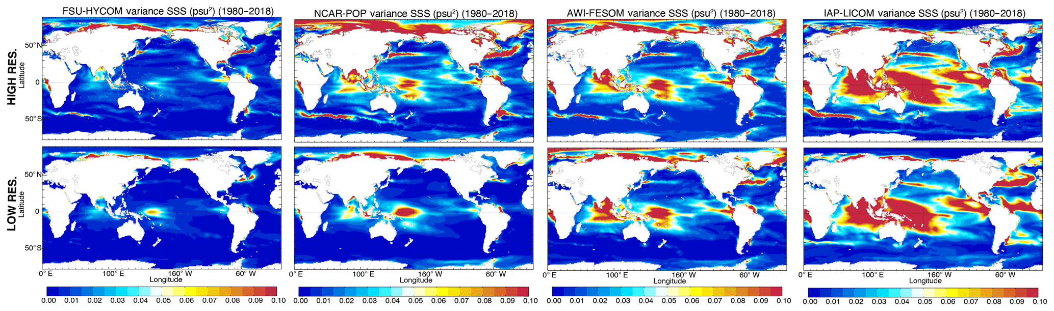
Figure 23Modeled and observed deseasonalized SSS variance.
While surface salinity generally exhibits globally enhanced variance at high resolution, particularly in the eddy-rich locations already highlighted above, the SSS variance plots are striking in that they show considerably more sensitivity to model formulation than to model horizontal resolution (Fig. 23). The increase in SSS variance at both resolutions across model systems – from FSU-HYCOM, to NCAR-POP, to AWI-FESOM, and to IAP-LICOM – is likely related to the steady increase in the surface-salinity-restoring timescale (Table 1). In the absence of reliable long-term global SSS observations, it is difficult to say which model formulation is best or whether high resolution improves the simulation of surface salinity variability.
4.3 Upper-ocean heat and salinity content mean biases and deseasonalized variance
The temperature and salinity distributions in the upper 700 m are less constrained to observations than the SST (which is restored to time-varying observed values through the sensible heat flux) and the SSS (which is restored to observed climatology through the artificial salinity-restoring flux). Therefore, vertically averaged upper-ocean heat content (UOHC) and salt content (UOSC) biases tend to be larger than surface biases, particularly at low latitudes (see Figs. 10, 24, and 25). The UK Met Office EN4 ocean analysis (Good et al., 2013) provides an observational benchmark for UOHC and UOSC mean and variance, but again considerable caution is warranted when interpreting model–observation discrepancies. The spatial resolution of this analysis is only 1∘, and it relaxes to climatology in data-sparse regions, which are extensive in the pre-Argo era (prior to 2000).
Both FSU-HYCOM and NCAR-POP show a significant and nearly ubiquitous mean bias reduction for UOHC and UOSC when resolution is increased (Figs. 24 and 25). In contrast, AWI-FESOM and IAP-LICOM show mixed results, with bias reduction in some regions (e.g., the Southern Ocean) offset by bias increase elsewhere. Regions of high observed UOHC variance include all the regions of high observed SST variance mentioned above as well as some variance hot spots in the subtropical western Pacific, the Tasman Sea, the subtropical south Indian Ocean, and the western tropical Atlantic (Fig. 24). The high-resolution models tend to show improved representation of these subsurface variance hot spots and enhanced variance in high EKE regions (western boundary currents, Agulhas, Southern Ocean, etc.). The high-resolution IAP-LICOM stands out for its globally high (perhaps unrealistically high) UOHC variance. This upper-ocean variance bias in IAP-LICOM is even more evident in UOSC (Fig. 25), although the limited sampling of 0–700 m salinity in the EN4 product implies that the observed variance estimate is almost certainly a gross underestimate. There is a hint (especially apparent in NCAR-POP and IAP-LICOM) of higher resolution resulting in enhanced salinity variance along subtropical cell spiciness pathways from the eastern extratropical Pacific to the tropical western Pacific (e.g., Yeager and Large, 2004).

Figure 24Top panels: mean 1980–2018 0–700 m temperature and variance from EN4. Middle panels: difference between the mean modeled 1980–2018 0–700 m temperature and EN4. Bottom panels: deseasonalized 0–700 m temperature modeled variance.
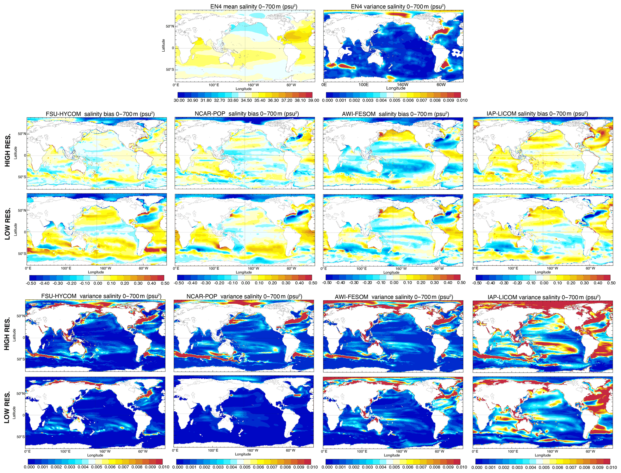
Figure 25Top panels: mean 1980–2018 0–700 m salinity and variance from EN4. Middle panels: difference between the mean modeled 1980–2018 0–700 m salinity and EN4. Bottom panels: deseasonalized 0–700 m salinity modeled variance.
4.4 Zonal AMOC mean and variance
Although the magnitude and temporal evolution of AMOC transport, as shown in Fig. 15a and b, differ significantly between different models and different horizontal resolutions, their time mean spatial structure and variance are quite similar among all the simulations as shown in Fig. 26 for the 1980 to 2018 period. All simulations show a positive upper cell and a negative lower cell. In the low-resolution simulations, the upper cell exhibits maximum transport near 1000 m and 35–40∘ N. The lower cell has its maximum transport near 3500–4000 m and is much weaker overall (∼ 2 Sv), except for IAP-LICOM (∼ 6 Sv in the subtropical North Atlantic). In high-resolution simulations, the upper cell extends deeper in all four models, which is more consistent with the observations, and the lower cell has a similar magnitude (2–4 Sv). This can be seen more clearly in Fig. 27, which compares the model AMOC profiles for 2004–2018 to the RAPID results near 26.5∘ N. South of about 20∘ N, the high-resolution AWI-FESOM exhibits a weak positive cell near the bottom that is unrealistic and is different from other models.
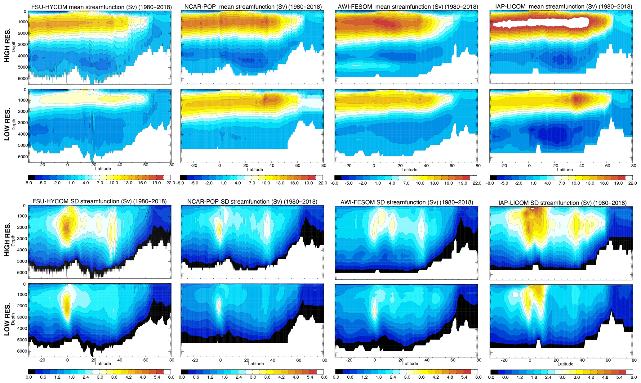
Figure 26Top panels: modeled time mean (1980–2018) Atlantic meridional overturning streamfunction ψz(yz) in the four models (low and high resolution). Lower panels: modeled standard deviation (1980–2018) of the Atlantic overturning streamfunction ψz(yz) derived from monthly mean fields.
The AMOC standard deviation shows a similar pattern between different resolutions and different models (Fig. 26). The variability is overall highest near the Equator (IAP-LICOM has the strongest variability near 10∘ N that differs from the other three). This is due to the large seasonal variability of the AMOC associated with the migration of the Intertropical Convergence Zone (ITCZ) and the changes in wind patterns and Ekman transport (Xu et al., 2014). The standard deviations based on annual means do not show such a maximum near the Equator (see Fig. 7 in Hirschi et al., 2020, for results based on different averaging scales). The variability is much weaker beyond the equatorial region. In the low-resolution simulations, the standard deviation is typically 2 Sv and has a slight elevation near 40∘ N. In the high-resolution simulations, the standard deviation is about 3 Sv and clearly shows a secondary maximum near 40∘ N. The difference between the low- and high-resolution simulations near 40∘ N highlights the impact of the meandering and mesoscale eddy variability of the Gulf Stream on AMOC variability.
Northward heat transport is usually correlated with higher AMOC transport in the Atlantic Ocean (e.g., Msadek et al., 2013; Xu et al., 2016). In the high-resolution experiments, there is also an overall reduction in subtropical Atlantic upper-ocean cold bias (Fig. 24), which can have an impact as shown by Msadek et al. (2013). Thus, it is not surprising that the high-resolution simulations have a higher heat transport in the Atlantic than the low-resolution counterparts (Fig. 28). The maximum northward heat transport at 20–30∘ N is about 1.0 PW in the high-resolution models, 0.6–0.8 PW in low-resolution models, and 1.25–1.3 PW in observations (Johns et al., 2011; Trenberth et al., 2019). In other basins such as the Indo-Pacific and the Southern Ocean, higher resolution does not necessarily lead to higher heat transport (Fig. 28a–c). But in general, the meridional heat transport in high resolution is closer to observations than the low-resolution simulations (Fig. 28).
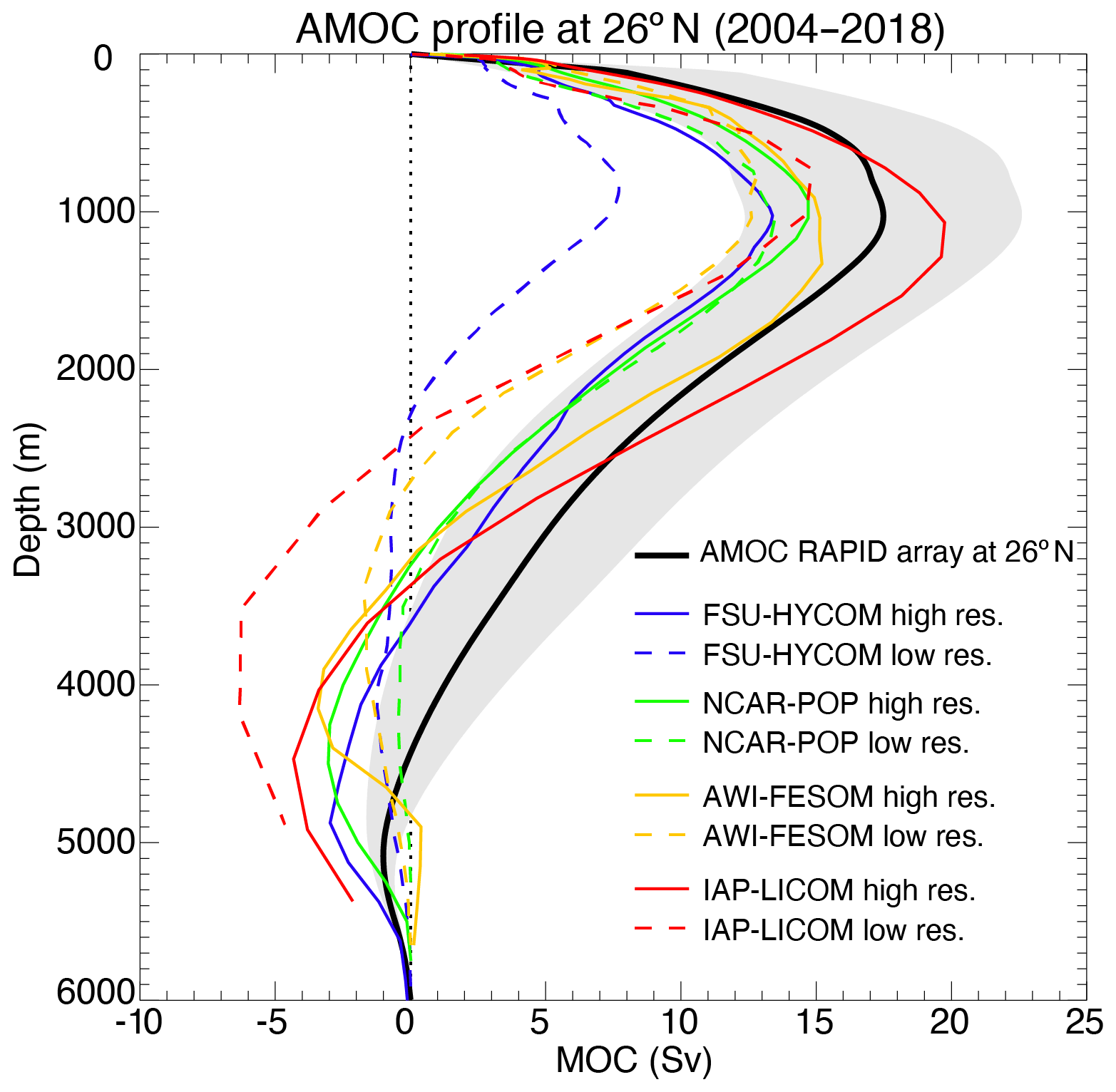
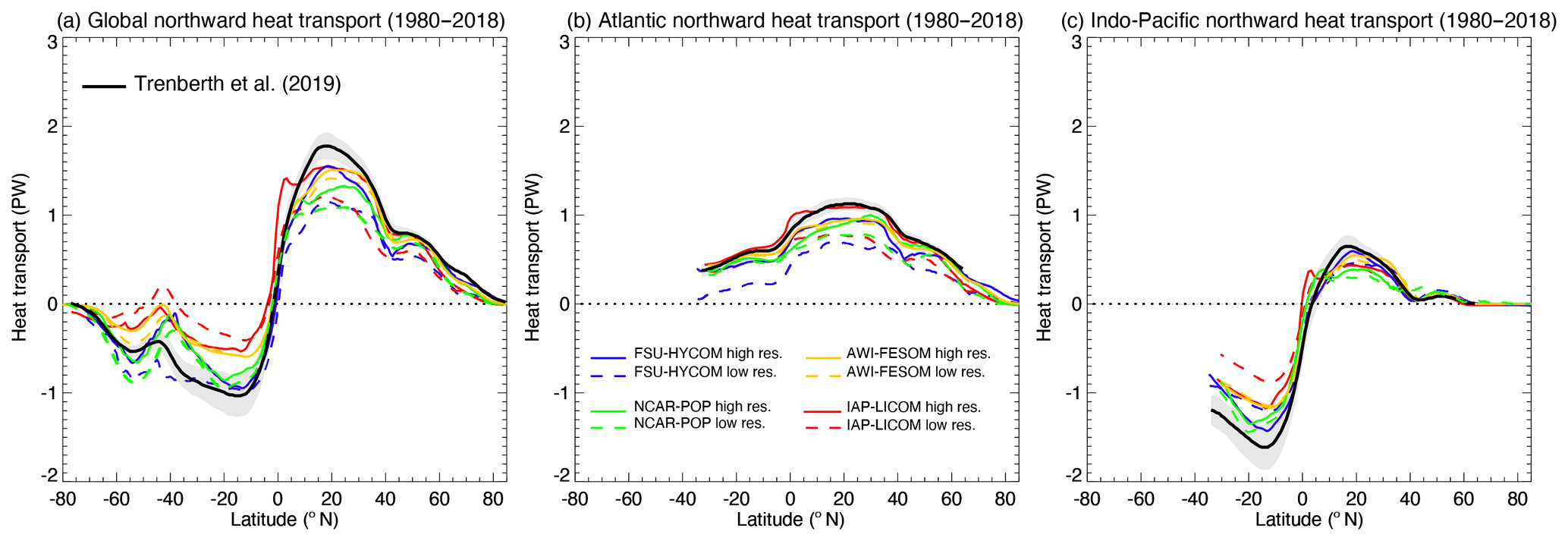
Figure 28Modeled time mean meridional heat transport in PW over 1980–2018: (a) global, (b) Atlantic Ocean, and (c) Indo-Pacific Ocean. Black lines are the latest observational results from Trenberth et al. (2019) with uncertainties.
4.5 Northern and Southern Hemisphere sea ice mean and variance
Figures 29–32 show 1980–2018 March and September modeled mean sea ice concentration (SIC) and sea ice thickness (SIT) together with the mean 1980–2018 SIC from passive microwave satellites and the mean 2003–2007 SIT from ICESat. As expected, given the relationship between sea ice extent and atmospheric temperature, the observed spatial pattern of winter SIC (averaged from 1980 to 2018) in the Northern Hemisphere (Fig. 29) is well-simulated in all the models at both low and high resolutions though with greater consistency among the high-resolution models. The position of the marginal ice zone (MIZ) – or areas where the SIC is between 15 % and 80 % – varies between models and resolutions. With the SIC close to 100 % in the interior Arctic in winter, the variance in modeled SIC (Figs. S1–S8) is small in March. The general pattern of the March Northern Hemisphere SIT is consistent between models, save for the IAP-LICOM, with increasing SIT towards the Canadian Archipelago. At both resolutions, AWI-FESOM presents slightly thicker sea ice throughout most of the Arctic Basin. The high-resolution IAP-LICOM is unrealistic, with very high sea ice thicknesses surrounding the pole. Figure 30 repeats Fig. 29, but for September. The comparison is similar: there are large inter-model differences in the MIZ, but there is a generally consistent pattern of increasing ice concentrations and thickness from the pole toward the Canadian Archipelago and northern Greenland. The location of the summer MIZ in FSU-HYCOM and NCAR-POP is too far away from the coast when compared to the observations and AWI-FESOM. Overall, there is a broad inter-model disagreement in SIT. The SIT variance (Figs. S1–S8) is higher in summer, especially in the shelf regions in experiments at both resolutions. While there is some sensitivity to model resolution for the simulated sea ice thickness, the difference due to changes in the resolution is smaller than the difference between the model results and the observations. Since the SIT observations shown in Figs. 29–32 are 2003–2007 averages, one may question the value of comparing the 2003–2007 ICESat observations to 1980–2018 averaged modeled fields. For a more direct comparison, the SIT modeled fields averaged from 2003 to 2007 are shown in Figs. S9 and S10 together with the ICESat observations when available, but they are almost identical to the 1980–2018 SIT fields shown in Figs. 29–32.
Figures 31–32 reproduce Figs. 29–30 for the Southern Hemisphere. The geographically simpler observed SIC in winter is well-represented by the models, with the exception of FSU-HYCOM, which simulates large regions of low ice concentration within the Antarctic pack. There is a clear difference in the modeled MIZ across the simulations: for example, it is wider in the low-resolution IAP-LICOM experiments when compared to the high-resolution experiment and vice versa for NCAR-POP. In the AWI-FESOM simulation, the MIZ is much narrower. The MIZ width is an important observable for explaining Southern Hemisphere sea ice concentration and thickness, largely determined by the presence of ocean surface waves (Kohout et al., 2014; Horvat et al., 2020). As none of the models allow for the propagation of ocean waves into the ice, the feedback between wave propagation and sea ice cover could not take place. In summer, SIT and SIC are poorly represented in FSU-HYCOM, NCAR-POP, and IAP-LICOM, which, at high resolution, produce an MIZ that is too wide (FSU-HYCOM, NCAR-POP) or no MIZ (IAP-LICOM) and inaccurately low representations of SIT, with most regions thinner than 20 cm. In general, observations indicate that areas of the most compact sea ice (Weddell Sea) are not those of the thickest ice (western Antarctic sector) in summer. None of the simulations adequately represent the observed relatively thick and noncompact sea ice in the western Antarctic. The high summer sea ice concentration in the Weddell and Ross Sea is only reasonably simulated in AWI-FESOM but with ice that is too thick. Although there is a high sensitivity to changing resolution in the Southern Hemisphere, the low- and high-resolution model pairs tend to agree more than the ensemble of low- or high-resolution models, indicating that sea ice model formulation differences may exceed the effects of resolution in these patterns. The models also show some sensitivity to the model resolution for the variance of the sea ice concentration and thickness in the Southern Hemisphere, especially in FSU-HYCOM. However, the difference between models is considerably larger. As IAP-LICOM significantly overestimates the sea ice thickness in its high-resolution setup, its variance is also much higher than the other models (Figs. S1–S8).
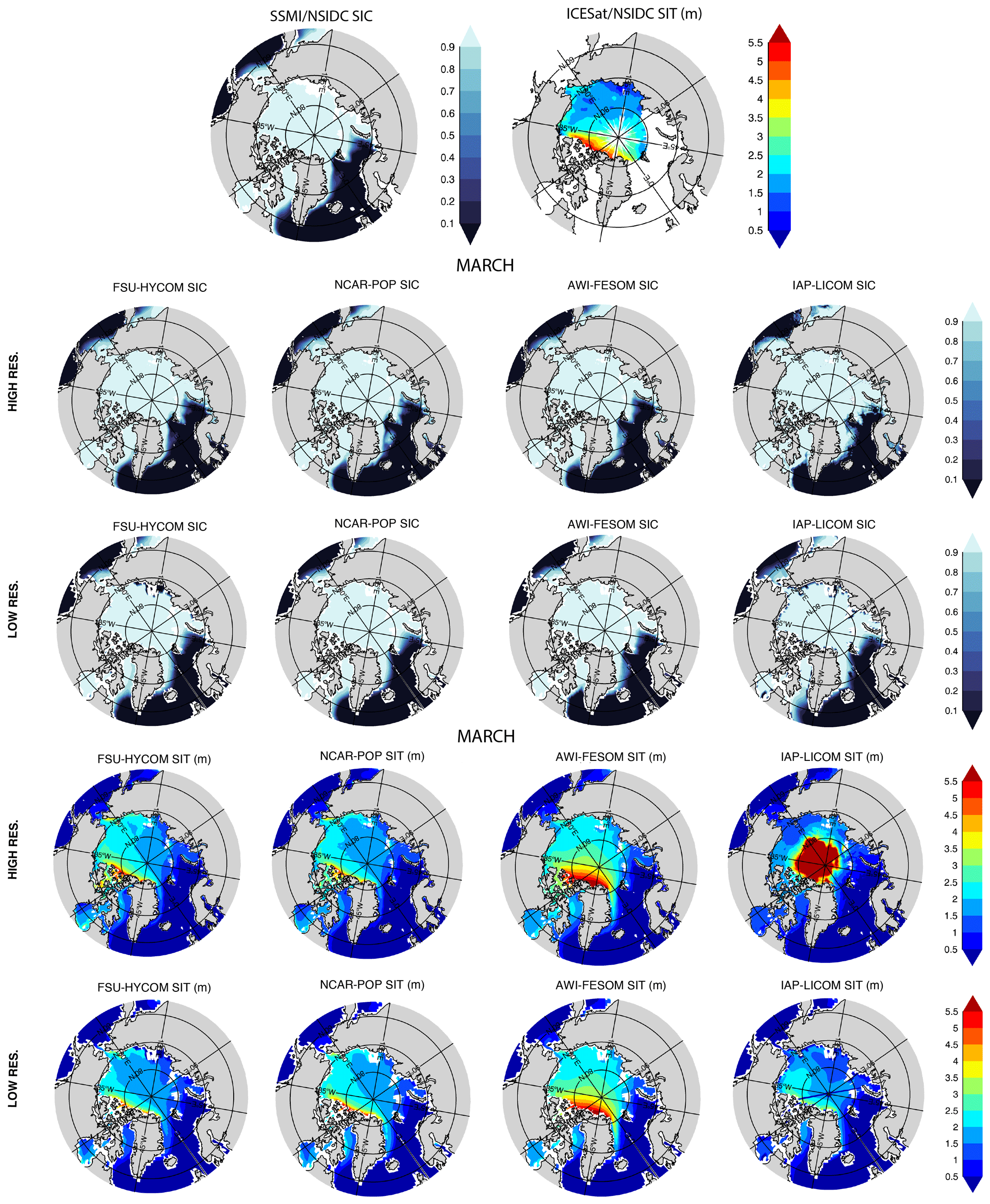
Figure 29Northern Hemisphere winter mean (March) sea ice concentration (SIC) and thickness (SIT). Top panels: 1980–2018 SIC from passive microwave satellites and 2003–2007 SIT from ICESat. Lower panels: 1980–2018 modeled SIC and SIT.

Figure 30Northern Hemisphere summer mean (September) sea ice concentration (SIC) and thickness (SIT). Top panel: 1980–2018 SIC from passive microwave satellites (summer SIT not available from ICESat). Lower panels: 1980–2018 modeled SIC and SIT.

Figure 31Southern Hemisphere winter mean (September) sea ice concentration (SIC) and thickness (SIT). Top panels: 1980–2018 SIC from passive microwave satellites and 2003–2007 SIT from ICESat. Lower panels: 1980–2018 modeled SIC and SIT.

Figure 32Southern Hemisphere summer mean (March) sea ice concentration (SIC) and thickness (SIT). Top panels: 1980–2018 SIC from passive microwave satellites and 2003–2007 SIT from ICESat. Lower panels: 1980–2018 modeled SIC and SIT.
The overall goal of this paper is to assess the robustness of climate-relevant improvements in ocean simulations (mean and variability) associated with moving from coarse (∼ 1∘) to eddy-resolving (∼ 0.1∘) horizontal resolutions. It also lays out a set of basic large-scale diagnostics for assessing the relative quality, variability, and sensitivity of high-resolution versus low-resolution ocean and sea ice models. The emphasis is on the key metrics used in climate modeling – SST, OHC, sea level, salinity, sea ice extent and volume, and circulations that tend to have global impacts (MOC, ACC, ITF) on the modeled climate. Here these metrics are assessed in a suite of four pairs of low-resolution–high-resolution ocean and sea ice models forced with the latest JRA55-do dataset (Tsujino et al., 2018). These results will provide a useful baseline for future process-focused analyses and ocean model development activities at diverse resolutions.
On the whole, the biases in the low-resolution variants are familiar and are similar in these models to those found when assessing sensitivity to forcing products (Tsujino et al., 2020). Gross features of the bias patterns in low-resolution models – position, strength, and variability of western boundary currents, equatorial currents, and ACC – are significantly improved in the high-resolution models. However, despite the fact that the high-resolution models “resolve” these features, the improvements in temperature and salinity are inconsistent among the different model families, and some regions show increased bias over their low-resolution counterparts. SSH variability and near-surface EKE are significantly – even qualitatively – improved in all high-resolution models over their low-resolution counterparts, although all of these models still underpredict the observed SSH variability and EKE, particularly in the ocean interior, which indicates a need for further refinements in resolution (Chassignet and Xu, 2017), and improvements in less dissipative subgrid schemes for high-resolution models (Pearson et al., 2017) are needed. The results in coupled models in the HighResMIP ensemble (Haarsma et al., 2016) show similar improvements in SSH and SST variability as well as EKE. Considerable differences in the high-resolution models used here were associated with the use of relative winds versus absolute winds. Renault et al. (2020) show that using relative winds contributes a feedback that tends to reduce EKE, and the models here are consistent with a 30 % or so reduction of EKE when relative winds are used.
One interesting aspect of the high-resolution models versus the low-resolution models was that the interannual variability in ACC and ITF transport as well as the AMOC was more consistent among the high-resolution models than among the low-resolution models. ITF transport was especially in agreement among the high-resolution models, indicating that better representation of the passageways through the Indonesian archipelago is critical. Consistency in all of these transports potentially indicates that higher-resolution models are needed to represent process variability, which may explain some of the past difficulties in comparing the magnitude of these phenomena across coarse-resolution models. However, the mean ACC transport and MOC strength were not in greater agreement among the high-resolution than the low-resolution models, which means that more work remains in evaluating sensitivity to numerics and subgrid-scale schemes for high-resolution models. Furthermore, Danabasoglu et al. (2016) note that low-resolution models come into greater agreement in AMOC variability after more cycles of the CORE forcing – this comparison was limited by the cost of the high-resolution models to only a single cycling of the forcing. It is unclear if the high-resolution models are in greater agreement only in the first cycle or generally. The short duration of a single forcing cycle limits the comparison of the decadal changes that are emphasized in Danabasoglu et al. (2016), so the improved agreement discussed here among high-resolution models is year by year rather than decade by decade. Nonetheless, the high-resolution models had systematically stronger and more variable AMOC, which was in better agreement with observations in both the maximum overturning and profile than the low-resolution models.
From a climate modeling perspective, ocean heat content, sea level, and sea ice stability are key metrics. There is some indication that the high-resolution models may warm more quickly below 700 m than the low-resolution models, indicating errors in parameterizations of vertical eddy heat transport. Griffies et al. (2016) found similar sensitivity to resolution in a model hierarchy, which they explained as resolved eddies versus parameterized eddies affecting vertical heat transport. However, warming between 0 and 700 m and global mean sea level rise were not systematically different across model families between the low-resolution and high-resolution models. Additional insights could be gained by computing vertical heat and salt budgets as in Griffies et al. (2015) and von Storch et al. (2016). Regional sea level rise, however, was significantly more variable in the high-resolution models wherein mesoscale eddies and the variability of western boundary and equatorial currents make an impact on regional sea level rise. Thus, it is critical to use high-resolution models to assess the ocean dynamic sea level (Gregory et al., 2019) contribution to regional sea level rise. Generally, there is a highly variable representation of sea ice with the exception of Arctic sea ice concentration – with high inter-model differences in sea ice thickness and volume, as well as generally inconsistent representation of sea ice in the Southern Hemisphere and sea ice thickness in the Arctic. Inter-model differences are larger than improvements with changing resolution – pointing to the known role of atmospheric forcing in setting modeled sea ice states and to the poor representation of sea ice physics and associated parameterizations. Sea ice concentration bias reduction is achievable, for example, through the inclusion of lateral melting and feedbacks between ice fracture and sea ice melting (Horvat and Tziperman, 2015; Roach et al., 2018, Bateson et al., 2020), but the wide spread in sea ice thickness and poor representation of Antarctic sea ice are known in CMIP-class models (Roach et al., 2020; Notz et al., 2020, Shu et al., 2020) and indicate that a fundamental overhaul of sea ice modeling may be needed.
Low-resolution versus high-resolution comparisons are often motivated by identifying persistent patterns across multiple models of bias or improvements with resolution. However, as is apparent in many metrics, there is no overall consistency among either the low-resolution or high-resolution ensemble from which to draw simplistic conclusions. This paper therefore does not dwell on the detailed differences among these models' numerics and parameterizations but is instead intended to serve as a benchmark for future studies comparing and improving different schemes in any of these models or similar ones. The numerics and parameterizations of these models are in continual development in both low-resolution and high-resolution versions. Ideally, however, one should strive to minimize the number of changes as the resolution is increased to ensure traceability. Other modeling centers have expressed interest in participating in this protocol in the future, and this paper provides a basis for comparison.
Finally, the models used in the present study are not coupled to active atmospheres, biospheres, land models, or land ice models. Thus, many important feedbacks and aspects of climate modeling are not addressed here. However, these same feedbacks complicate diagnosis of the source of model biases and resolution sensitivity, which is where this study intends to contribute.
The forcing dataset for OMIP-2 is available through input4MIPs (https://esgf-node.llnl.gov/search/input4mips/, last access: 21 September 2020) – see Table S1 in the Supplement for a list of the files. An archive of the model outputs and the scripts used to process data and generate figures are available at https://doi.org/10.5281/zenodo.3934822 (Chassignet et al., 2020b). For the observed sea ice concentration, the data are available at https://doi.org/10.5067/EYICLBOAAJOU (Stroeve and Meier, 2017). For the observed sea ice thickness, the data are available at https://doi.org/10.5067/SXJVJ3A2XIZT (Yi and Zwally, 2009) and at https://earth.gsfc.nasa.gov/index.php/cryo/data/antarctic-sea-ice-thickness (last access: 21 September 2020; Kurtz and Markus, 2012) for the Arctic and Antarctic, respectively.
The supplement related to this article is available online at: https://doi.org/10.5194/gmd-13-4595-2020-supplement.
EC, SY, and BFK proposed and led this evaluation study. AB processed the model outputs and produced the figures. The following authors are responsible for the individual models, simulations, and diagnostics: AB, XX, and EPC for FSU-HYCOM; SY, FC, WK, and GD for NCAR-POP; QW, SD, NK, and DS for AWI-FESOM; HL, YL, and PL for IAP-LICOM3. CH contributed to the sea ice sections. All authors contributed to the writing and editing processes.
The authors declare that they have no conflict of interest.
The authors would like to thank the two anonymous reviewers and the editor for their constructive comments. The FSU contribution was supported by the National Oceanic and Atmospheric Administration (NOAA) Earth System Prediction Capability Project (award no. NA15OAR4320064), the NOAA Climate Program Office (CPO) MAPP Program (award no. 5NA15OAR4310088), and the US National Science Foundation (NSF) Physical Oceanography Program (award no. 1537136). The NCAR contribution was supported by the NOAA CPO Climate Variability and Predictability (CVP) Program. NCAR is a major facility sponsored by NSF under cooperative agreement no. 1852977. The AWI contribution was supported by projects S1 (Diagnosis and Metrics in Climate Models) and S2 (Improved Parameterizations and Numerics in Climate Models) of the Collaborative Research Centre TRR 181 “Energy Transfer in Atmosphere and Ocean” funded by the Deutsche Forschungsgemeinschaft (DFG, German Research Foundation; project no. 274762653), the Helmholtz Climate Initiative REKLIM (Regional Climate Change), and the European Union Horizon 2020 Research and Innovation program through grant agreement no. 727862 APPLICATE. The IAP contribution was supported by the National Natural Science Foundation of China (grant nos. 41931183 and 41976026). Dmitry Sein was supported by the Ministry of Science and Higher Education of Russia (theme no. 0149-2019-0015). Baylor Fox-Kemper's contribution was supported by the NSF Physical Oceanography Program (award no. 1350795), the Office of Naval Research (grant no. N00014-17-1-2393), and NOAA (award no. NA19OAR4310366).
This research has been supported by NOAA (award nos. NA15OAR4320064, 5NA15OAR4310088, and NA19OAR4310366), the NSF (award nos. 1350795, 1537136, and 1852977), the ONR (grant no. N00014-17-1-2393), the Deutsche Forschungsgemeinschaft (grant no. 274762653), European Union Horizon 2020 (grant no. 727862 APPLICATE), the the Ministry of Science and Higher Education of Russia (theme no. 0149-2019-0015), and the National Natural Science Foundation of China (grant nos. 41931183 and 41976026).
This paper was edited by Julia Hargreaves and reviewed by two anonymous referees.
Ajayi, A., Le Sommer, J., Chassignet, E., Molines, J.-M., Xu, X., Albert, A., and Cosme, E.: Spatial and temporal variability of the North Atlantic eddy field from two kilometric-resolution ocean models, J. Geophy. Res.-Oceans, 125, e2019JC015827, https://doi.org/10.1029/2019JC015827, 2020.
Bamber, J. L., Tedstone, A. J., King, M. D., Howat, I. M., Enderlin, E. M., van den Broeke, M. R., and Noel, B.: Land ice freshwater budget of the Arctic and North Atlantic Oceans: 1. Data, methods, and results, J. Geophys. Res.-Oceans, 123, 1827–1837, https://doi.org/10.1002/2017JC013605, 2018.
Bamber, J., van den Broeke, M., Ettema, J., Lenaerts, J., and Rignot, E.: Recent large increases in freshwater fluxes from Greenland into the North Atlantic, Geophys. Res. Lett., 39, L19501, https://doi.org/10.1029/2012GL052552, 2012.
Banzon, V. F., Reynolds, R. W., Stokes, D., and Xue, Y.: A 1/4∘ spatial-resolution daily sea surface temperature climatology based on a blended satellite and in situ analysis, J. Climate, 27, 8221–8228, https://doi.org/10.1175/JCLI-D-14-00293.1, 2014.
Bao, Q., Lin, P., Zhou, T., Liu, Y., Yu, Y., Wu, G., He, B., He, J., Li, L., Li, J., Li, Y., Liu, H., Qiao, F., Song, Z., Wang, B., Wang, J., Wang, P., Wang, X., Wang, Z., Wu, B., Wu, T., Xu, Y., Yu, H., Zhao, W., Zheng, W., and Zhou, L.: The Flexible Global Ocean-Atmosphere-Land system model, Spectral Version 2: FGOALS-s2, Adv. Atmos. Sci., 30, 561–576, https://doi.org/10.1007/s00376-012-2113-9, 2013.
Baringer, M. O. and Garzoli, S. L.: Meridional heat transport determined with expendable bathythermographs-Part I: Error estimates from model and hydrographic data, Deep-Sea Res. Pt. I, 54, 1390–1401, https://doi.org/10.1016/j.dsr.2007.03.011, 2007.
Bateson, A. W., Feltham, D. L., Schröder, D., Hosekova, L., Ridley, J. K., and Aksenov, Y.: Impact of sea ice floe size distribution on seasonal fragmentation and melt of Arctic sea ice, The Cryosphere, 14, 403–428, https://doi.org/10.5194/tc-14-403-2020, 2020.
Bleck, R.: An oceanic general circulation model framed in hybrid isopycnic-Cartesian coordinates, Ocean Model., 4, 55–88, https://doi.org/10.1016/S1463-5003(01)00012-9, 2002.
Böning, C. W., Scheinert, M., Dengg, J., Biastoch, A., and Funk, A.: Decadal variability of subpolar gyre transport and its reverberation in the North Atlantic overturning, Geophys. Res. Lett., 33, L21S01, https://doi.org/10.1029/2006GL026906, 2006.
Bryan, F. O., Tomas, R., Dennis, J. M., Chelton, D. B., Loeb, N. G., and McClean, J. L.: Frontal Scale Air–Sea Interaction in High-Resolution Coupled Climate Models, J. Climate, 23, 6277–6291, https://doi.org/10.1175/2010JCLI3665.1, 2010.
Callies, J., Flierl, G., Ferrari, R., and Fox-Kemper, B.: The role of mixed-layer instabilities in submesoscale turbulence, J. Fluid Mech., 788, 5–41, https://doi.org/10.1017/jfm.2015.700, 2016.
Canuto, V. M., Howard, A., Cheng, Y., and Dubovikov, M. S.: Ocean turbulence. Part I: One-point closure model–momentum and heat vertical diffusivities, J. Phys. Oceanogr., 31, 1413–1426, https://doi.org/10.1175/1520-0485(2001)031<1413:OTPIOP>2.0.CO;2, 2001.
Canuto, V. M., Howard, A., Cheng, Y., and Dubovikov, M. S.: Ocean turbulence. Part II: Vertical diffusivities of momentum, heat, salt, mass, and passive scalars, J. Phys. Oceanogr., 32, 240–264, https://doi.org/10.1175/1520-0485(2002)032<0240:OTPIVD>2.0.CO;2, 2002.
Carnes, M., Helber, R. W., Barron, C. N., and Dastugue, J. M.: Validation test report for GDEM4, Technical Report NRL, Stennis, MS, 66 pp., 2010.
Chassignet, E. P., Smith, L. T., Halliwell, G. R., and Bleck, R.: North Atlantic simulations with the Hybrid Coordinate Ocean Model (HYCOM): Impact of the vertical coordinate choice, reference pressure, and thermobaricity, J. Phys. Oceanogr., 33, 2504–2526, https://doi.org/10.1175/1520-0485(2003)033<2504:NASWTH>2.0.CO;2, 2003.
Chassignet, E. P. and Marshall, D. P.: Gulf Stream separation in numerical ocean models, in: Geophysical Monograph Series, 177, 39–61, 2008.
Chassignet, E. P. and Xu, X.: Impact of horizontal resolution (1/12∘ to 1/50∘) on Gulf Stream separation, penetration, and variability, J. Phys. Oceanogr., 47, 1999–2021, https://doi.org/10.1175/JPO-D-17-0031.1, 2017.
Chassignet, E. P., Yeager, S. G., Fox-Kemper, B., Bozec, A., Castruccio, F., Danabasoglu, G., Kim, W. M., Koldunov, N., Li, Y., Lin, P., Liu, H., Sein, D., Sidorenko, D., Wang, Q., and Xu, X.: Impact of horizontal resolution on the energetics of global ocean-sea-ice model simulations, CLIVAR Variations/Exchanges, 18, 23–30, https://doi.org/10.5065/g8w0-fy32, 2020a.
Chassignet, E. P., Yeager, S. G., Fox-Kemper, B., Bozec, A., Castruccio, F., Danabasoglu, G., Kim, W. M., Koldunov, N., Li, Y., Lin, P., Liu, H., Sein, D., Sidorenko, D., Wang, Q., and Xu, X.: Impact of horizontal resolution on global ocean-sea-ice model simulations based on the experimental protocols of the Ocean Model Intercomparison Project phase 2 (OMIP-2) (Version v2.0) [Data set], Geoscientific Model Development, Zenodo, https://doi.org/10.5281/zenodo.3934822, 2020b.
Chidichimo, M. P., Donohue, K. A., Watts, D. R., and Tracey, K. L.: Baroclinic transport time series of the Antarctic Circumpolar Current measured in Drake Passage, J. Phys. Oceanogr., 44, 1829–1853, https://doi.org/10.1175/JPO-D-13-071.1, 2014.
Craig, A. P., Vertenstein, M., and Jacob, R.: A new flexible coupler for earth system modeling developed for CCSM4 and CESM1, Int. J. High Perform. Comput. Appl., 26, 31–42, https://doi.org/10.1177/1094342011428141, 2012.
Cunningham, S. A.: Transport and variability of the Antarctic Circumpolar Current in Drake Passage, J. Geophys. Res., 108, 8084, https://doi.org/10.1029/2001JC001147, 2003.
Danabasoglu, G., Bates, S. C., Briegleb, B. P., Jayne, S. R., Jochum, M., Large, W. G., Peacock, S., and Yeager, S. G.: The CCSM4 Ocean Component, J. Climate, 25, 1361–1389, https://doi.org/10.1175/JCLI-D-11-00091.1, 2012.
Danabasoglu, G., Ferrari, R., and McWilliams, J. C.: Sensitivity of an ocean general circulation model to a parameterization of near-surface eddy fluxes, J. Climate, 21, 1192–1208, https://doi.org/10.1175/2007JCLI1508.1, 2008.
Danabasoglu, G., Large, W. G., and Briegleb, B. P.: Climate impacts of parameterized Nordic Sea overflows, J. Geophys. Res., 115, C11005, https://doi.org/10.1029/2010JC006243, 2010.
Danabasoglu, G. and Marshall, J.: Effects of vertical variations of thickness diffusivity in an ocean general circulation model, Ocean Model., 18, 122–141, https://doi.org/10.1016/j.ocemod.2007.03.006, 2007.
Danabasoglu, G., Yeager, S. G., Bailey, D., Behrens, E., Bentsen, M., Bi, D., Biastoch, A., Böning, C., Bozec, A., Canuto, V. M., Cassou, C., Chassignet, E., Coward, A. C., Danilov, S., Diansky, N., Drange, H., Farneti, R., Fernandez, E., Fogli, P. G., Forget, G., Fujii, Y., Griffies, S. M., Gusev, A., Heimbach, P., Howard, A., Jung, T., Kelley, M., Large, W. G., Leboissetier, A., Lu, J., Madec, G., Marsland, S. J., Masina, S., Navarra, A., George Nurser, A. J., Pirani, A., y Mélia, D. S., Samuels, B. L., Scheinert, M., Sidorenko, D., Treguier, A. M., Tsujino, H., Uotila, P., Valcke, S., Voldoire, A., and Wang, Q.: North Atlantic simulations in Coordinated Ocean-ice Reference Experiments phase II (CORE-II). Part I: Mean states, Ocean Model., 73, 76–107, https://doi.org/10.1016/j.ocemod.2013.10.005, 2014.
Danabasoglu, G., Yeager, S. G., Kim, W. M., Behrens, E., Bentsen, M., Bi, D., Biastoch, A., Bleck, R., Böning, C., Bozec, A., Canuto, V. M., Cassou, C., Chassignet, E., Coward, A. C., Danilov, S., Diansky, N., Drange, H., Farneti, R., Fernandez, E., Fogli, P. G., Forget, G., Fujii, Y., Griffies, S. M., Gusev, A., Heimbach, P., Howard, A., Ilicak, M., Jung, T., Karspeck, A. R., Kelley, M., Large, W. G., Leboissetier, A., Lu, J., Madec, G., Marsland, S. J., Masina, S., Navarra, A., Nurser, A. J. G., Pirani, A., Romanou, A., David, S. y. M., Samuels, B. L., Scheinert, M., Sidorenko, D., Sun, S., Treguier, A. M., Tsujino, H., Uotila, P., Valcke, S., Voldoire, A., Wang, Q., and Yashayaev, I.: North Atlantic simulations in Coordinated Ocean-ice Reference Experiments phase II (CORE-II). Part II: Inter-annual to decadal variability, Ocean Model., 97, 65–90, https://doi.org/10.1016/j.ocemod.2015.11.007, 2016.
Danabasoglu, G., Lamarque, J. -F., Bachmeister, J., Bailey, D. A., DuVivier, A. K., Edwards, J., Emmons, L. K., Fasullo, J., Garcia, R., Gettelman, A., Hannay, C., Holland, M. M., Large, W. G., Lawrence, D. M., Lenaerts, J. T. M., Lindsay, K., Lipscomb, W. H., Mills, M. J., Neale, R., Oleson, K. W., Otto-Bliesner, B., Phillips, A. S., Sacks, W., Tilmes, S., van Kampenhout, L., Vertenstein, M., Bertini, A., Dennis, J., Deser, C., Fischer, C., Fox-Kember, B., Kay, J. E., Kinnison, D., Kushner, P. J., Long, M. C., Mickelson, S., Moore, J. K., Nienhouse, E., Polvani, L., Rasch, P. J., and Strand, W. G.: The Community Earth System Model version 2 (CESM2), J. Adv. Model. Earth Sys., 12, e2019MS001916, https://doi.org/10.1029/2019MS001916, 2020.
Danilov, S., Wang, Q., Timmermann, R., Iakovlev, N., Sidorenko, D., Kimmritz, M., Jung, T., and Schröter, J.: Finite-Element Sea Ice Model (FESIM), version 2, Geosci. Model Dev., 8, 1747–1761, https://doi.org/10.5194/gmd-8-1747-2015, 2015.
Danilov, S., Kivman, G., and Schröter, J.: A finite-element ocean model: Principles and evaluation, Ocean Model., 6, 125–150, https://doi.org/10.1016/S1463-5003(02)00063-X, 2004.
Depoorter, M. A., Bamber, J. L., Griggs, J. A., Lenaerts, J. T. M., Ligtenberg, S. R. M., Van Den Broeke, M. R., and Moholdt, G.: Calving fluxes and basal melt rates of Antarctic ice shelves, Nature, 502, 89–92, https://doi.org/10.1038/nature12567, 2013.
Dong, S., Baringer, M. O., Goni, G. J., Meinen, C. S., and Garzoli, S. L.: Seasonal variations in the South Atlantic Meridional Overturning Circulation from observations and numerical models, Geophys. Res. Lett., 41, 4611–4618, https://doi.org/10.1002/2014GL060428, 2014.
Dong, S., Garzoli, S., Baringer, M., Meinen, C., and Goni, G.: Interannual variations in the Atlantic meridional overturning circulation and its relationship with the net northward heat transport in the South Atlantic, Geophys. Res. Lett., 36, L20606, https://doi.org/10.1029/2009GL039356, 2009.
Dong, S., Goni, G., and Bringas, F.: Temporal variability of the South Atlantic Meridional Overturning Circulation between 20∘ S and 35∘ S, Geophys. Res. Lett., 42, 7655–7662, https://doi.org/10.1002/2015GL065603, 2015.
Donohue, K. A., Tracey, K. L., Watts, D. R., Chidichimo, M. P., and Chereskin, T. K.: Mean Antarctic Circumpolar Current transport measured in Drake Passage, Geophys. Res. Lett., 43, 11760–11767, https://doi.org/10.1002/2016GL070319, 2016.
Downes, S. M., Farneti, R., Uotila, P., Griffies, S. M., Marsland, S. J., Bailey, D., Behrens, E., Bentsen, M., Bi, D., Biastoch, A., Böning, C., Bozec, A., Canuto, V. M., Chassignet, E., Danabasoglu, G., Danilov, S., Diansky, N., Drange, H., Fogli, P. G., Gusev, A., Howard, A., Ilicak, M., Jung, T., Kelley, M., Large, W. G., Leboissetier, A., Long, M., Lu, J., Masina, S., Mishra, A., Navarra, A., George Nurser, A. J., Patara, L., Samuels, B. L., Sidorenko, D., Spence, P., Tsujino, H., Wang, Q., and Yeager, S. G.: An assessment of Southern Ocean water masses and sea ice during 1988-2007 in a suite of interannual CORE-II simulations, Ocean Model., 94, 67–94, https://doi.org/10.1016/j.ocemod.2015.07.022, 2015.
Eyring, V., Bony, S., Meehl, G. A., Senior, C. A., Stevens, B., Stouffer, R. J., and Taylor, K. E.: Overview of the Coupled Model Intercomparison Project Phase 6 (CMIP6) experimental design and organization, Geosci. Model Dev., 9, 1937–1958, https://doi.org/10.5194/gmd-9-1937-2016, 2016.
Farneti, R., Downes, S. M., Griffies, S. M., Marsland, S. J., Behrens, E., Bentsen, M., Bi, D., Biastoch, A., Böning, C., Bozec, A., Canuto, V. M., Chassignet, E., Danabasoglu, G., Danilov, S., Diansky, N., Drange, H., Fogli, P. G., Gusev, A., Hallberg, R. W., Howard, A., Ilicak, M., Jung, T., Kelley, M., Large, W. G., Leboissetier, A., Long, M., Lu, J., Masina, S., Mishra, A., Navarra, A., George Nurser, A. J., Patara, L., Samuels, B. L., Sidorenko, D., Tsujino, H., Uotila, P., Wang, Q., and Yeager, S. G.: An assessment of Antarctic Circumpolar Current and Southern Ocean meridional overturning circulation during 1958–2007 in a suite of interannual CORE-II simulations, Ocean Model., 93, 84–120, https://doi.org/10.1016/j.ocemod.2015.07.009, 2015.
Ferrari, R., McWilliams, J. C., Canuto, V. M., and Dubovikov, M.: Parameterization of eddy fluxes near oceanic boundaries, J. Climate, 21, 2770–2789, https://doi.org/10.1175/2007JCLI1510.1, 2008.
Ferreira, D., Marshall, J., and Heimbach, P.: Estimating eddy stresses by fitting dynamics to observations using a residual-mean ocean circulation model and its adjoint, J. Phys. Oceanogr., 35, 1891–1910, https://doi.org/10.1175/JPO2785.1, 2005.
Fetterer, F., Knowles, K., Meier, W., Savoie, M., and Windnagel, A. K.: Sea Ice Index, Version 3, Boulder, CO, USA, 2017.
Firing, Y. L., Chereskin, T. K., and Mazloff, M. R.: Vertical structure and transport of the Antarctic Circumpolar Current in Drake Passage from direct velocity observations, J. Geophys. Res., 116, C08015, https://doi.org/10.1029/2011JC006999, 2011.
Fox-Kemper, B., Danabasoglu, G., Ferrari, R., Griffies, S. M., Hallberg, R. W., Holland, M. M., Maltrud, M. E., Peacock, S., and Samuels, B. L.: Parameterization of mixed layer eddies. III: Implementation and impact in global ocean climate simulations, Ocean Model., 39, 61–78, https://doi.org/10.1016/j.ocemod.2010.09.002, 2011.
Fox-Kemper, B., Adcroft, A., Böning, C. W., Chassignet, E. P., Curchitser, E., Danabasoglu, G., Eden, C., England, M. H., Gerdes, R., Greatbatch, R. J., Griffies, S. M., Hallberg, R. W., Hanert, E., Heimbach, P., Hewitt, H. T., Hill, C. N., Komuro, Y., Legg, S., Sommer, J. Le, Masina, S., Marsland, S. J., Penny, S. G., Qiao, F., Ringler, T. D., Treguier, A. M., Tsujino, H., Uotila, P., and Yeager, S. G.: Challenges and prospects in ocean circulation models, Front. Mar. Sci., 6, 65, https://doi.org/10.3389/fmars.2019.00065, 2019.
Fox-Kemper, B., Ferrari, R., and Hallberg, R.: Parameterization of mixed layer eddies. Part I: Theory and diagnosis, J. Phys. Oceanogr., 38, 1145–1165, https://doi.org/10.1175/2007JPO3792.1, 2008.
Garzoli, S. L., Baringer, M. O., Dong, S., Perez, R. C., and Yao, Q.: South Atlantic meridional fluxes, Deep-Sea Res. Pt. I, 71, 21–32, https://doi.org/10.1016/j.dsr.2012.09.003, 2013.
Gent, P. R. and Danabasoglu, G.: Response to increasing southern hemisphere winds in CCSM4, J. Climate, 24, 4992–4998, https://doi.org/10.1175/JCLI-D-10-05011.1, 2011.
Gent, P. R. and Mcwilliams, J. C.: Isopycnal mixing in ocean circulation models, J. Phys. Oceanogr., 20, 150–155, https://doi.org/10.1175/1520-0485(1990)020<0150:imiocm>2.0.co;2, 1990.
Godfrey, J. S.: A Sverdrup model of the depth-integrated flow for the world ocean allowing for island circulations, Geophys. Astrophys. Fluid Dyn., 45, 89–112, https://doi.org/10.1080/03091928908208894, 1989.
Goes, M., Goni, G., and Dong, S.: An optimal XBT-based monitoring system for the South Atlantic meridional overturning circulation at 34∘ S, J. Geophys. Res.-Oceans, 120, 161–181, https://doi.org/10.1002/2014JC010202, 2015.
Good, S. A., Martin, M. J., and Rayner, N. A.: EN4: Quality controlled ocean temperature and salinity profiles and monthly objective analyses with uncertainty estimates, J. Geophys. Res.-Oceans, 118, 6704–6716, https://doi.org/10.1002/2013JC009067, 2013.
Gordon, A. L., Sprintall, J., Van Aken, H. M., Susanto, R. D., Wijffels, S., Molcard, R., Ffield, A., Pranowo, W., and Wirasantosa, S.: The Indonesian throughflow during 2004–2006 as observed by the INSTANT program, Dyn. Atmos. Ocean., 50, 115–128, https://doi.org/10.1016/j.dynatmoce.2009.12.002, 2010.
Gordon, A. L.: Oceanography of the Indonesian seas and their throughflow, Oceanography, 18, 15–27, https://doi.org/10.5670/oceanog.2005.01, 2005.
Gordon, A. L.: Interocean exchange of thermocline water, J. Geophys. Res., 91, 5037, https://doi.org/10.1029/jc091ic04p05037, 1986.
Gregory, J. M., Griffies, S. M., Hughes, C. W., Lowe, J. A., Church, J. A., Fukimori, I., Gomez, N., Kopp, R. E., Landerer, F., Cozannet, G. Le, Ponte, R. M., Stammer, D., Tamisiea, M. E., and van de Wal, R. S. W.: Concepts and terminology for sea level: Mean, variability and change, both local and global, Surv. Geophys., 40, 1251–1289, https://doi.org/10.1007/s10712-019-09525-z, 2019.
Griffies, S. M.: The Gent–McWilliams Skew Flux, J. Phys. Oceanogr., 28, 831–841, https://doi.org/10.1175/1520-0485(1998)028<0831:TGMSF>2.0.CO;2, 1998.
Griffies, S. M., Biastoch, A., Böning, C., Bryan, F., Danabasoglu, G., Chassignet, E. P., England, M. H., Gerdes, R., Haak, H., Hallberg, R. W., Hazeleger, W., Jungclaus, J., Large, W. G., Madec, G., Pirani, A., Samuels, B. L., Scheinert, M., Gupta, A. Sen, Severijns, C. A., Simmons, H. L., Treguier, A. M., Winton, M., Yeager, S., and Yin, J.: Coordinated Ocean-ice Reference Experiments (COREs), Ocean Model., 26, 1–46, https://doi.org/10.1016/j.ocemod.2008.08.007, 2009.
Griffies, S. M., Yin, J., Durack, P. J., Goddard, P., Bates, S. C., Behrens, E., Bentsen, M., Bi, D., Biastoch, A., Böning, C. W., Bozec, A., Chassignet, E., Danabasoglu, G., Danilov, S., Domingues, C. M., Drange, H., Farneti, R., Fernandez, E., Greatbatch, R. J., Holland, D. M., Ilicak, M., Large, W. G., Lorbacher, K., Lu, J., Marsland, S. J., Mishra, A., George Nurser, A. J., Salas y Mélia, D., Palter, J. B., Samuels, B. L., Schröter, J., Schwarzkopf, F. U., Sidorenko, D., Treguier, A. M., Tseng, Y. heng, Tsujino, H., Uotila, P., Valcke, S., Voldoire, A., Wang, Q., Winton, M., and Zhang, X.: An assessment of global and regional sea level for years 1993–2007 in a suite of interannual CORE-II simulations, Ocean Model., 78, 35–89, https://doi.org/10.1016/j.ocemod.2014.03.004, 2014.
Griffies, S. M., Winton, M., Anderson, W. G., Benson, R., Delworth, T. L., Dufour, C. O., Dunne, J. P., Goddard, P., Morrison, A. K., Rosati, A., Wittenberg, A. T., Yin, J. J., and Zhang, R.: Impacts on ocean heat from transient mesoscale eddies in a hierarchy of climate models, J. Climate, 28, 952–977, 2015.
Griffies, S. M., Danabasoglu, G., Durack, P. J., Adcroft, A. J., Balaji, V., Böning, C. W., Chassignet, E. P., Curchitser, E., Deshayes, J., Drange, H., Fox-Kemper, B., Gleckler, P. J., Gregory, J. M., Haak, H., Hallberg, R. W., Heimbach, P., Hewitt, H. T., Holland, D. M., Ilyina, T., Jungclaus, J. H., Komuro, Y., Krasting, J. P., Large, W. G., Marsland, S. J., Masina, S., McDougall, T. J., Nurser, A. J. G., Orr, J. C., Pirani, A., Qiao, F., Stouffer, R. J., Taylor, K. E., Treguier, A. M., Tsujino, H., Uotila, P., Valdivieso, M., Wang, Q., Winton, M., and Yeager, S. G.: OMIP contribution to CMIP6: experimental and diagnostic protocol for the physical component of the Ocean Model Intercomparison Project, Geosci. Model Dev., 9, 3231–3296, https://doi.org/10.5194/gmd-9-3231-2016, 2016.
Haarsma, R. J., Roberts, M. J., Vidale, P. L., Senior, C. A., Bellucci, A., Bao, Q., Chang, P., Corti, S., Fučkar, N. S., Guemas, V., von Hardenberg, J., Hazeleger, W., Kodama, C., Koenigk, T., Leung, L. R., Lu, J., Luo, J.-J., Mao, J., Mizielinski, M. S., Mizuta, R., Nobre, P., Satoh, M., Scoccimarro, E., Semmler, T., Small, J., and von Storch, J.-S.: High Resolution Model Intercomparison Project (HighResMIP v1.0) for CMIP6, Geosci. Model Dev., 9, 4185–4208, https://doi.org/10.5194/gmd-9-4185-2016, 2016.
Häkkinen, S. and Rhines, P. B.: Decline of Subpolar North Atlantic Circulation during the 1990s, Science, 304, 555–559, https://doi.org/10.1126/science.1094917, 2004.
Hallberg, R.: Using a resolution function to regulate parameterizations of oceanic mesoscale eddy effects, Ocean Model., 72, 92–103, https://doi.org/10.1016/j.ocemod.2013.08.007, 2013.
Hallberg, R. and Gnanadesikan, A.: The role of Eddies in determining the structure and response of the wind-driven Southern hemisphere overturning: Results from the Modeling Eddies in the Southern Ocean (MESO) project, J. Phys. Oceanogr., 36, 2232–2252, https://doi.org/10.1175/JPO2980.1, 2006.
Halliwell, G. R.: Evaluation of vertical coordinate and vertical mixing algorithms in the HYbrid-Coordinate Ocean Model (HYCOM), Ocean Model., 7, 285–322, https://doi.org/10.1016/j.ocemod.2003.10.002, 2004.
Hirschi, J. J.-M., Barnier, B., Böning, C., Biastoch, A., Blaker, A. T., Coward, A., Danilov, S., Drijfhout, S., Getzlaff, K., Griffies, S. M., Hasumi, H., Hewitt, H., Iovino, D., Kawasaki, T., Kiss, A. E., Koldunov, N., Marzocchi, A., Moat, B., Molines, J.-M., Myers, P. G., Penduff, T., Roberts, M., Treguier, A.-M., Sein, D. V., Sidorenko, D., Small1, J., Spence, P., Thompson, L., Weijer, W., and Xu, X.: The Atlantic meridional overturning circulation in high resolution models, J. Geophys. Res.-Oceans, 125, e2019JC015522, https://doi.org/10.1029/2019JC015522, 2020.
Horvat, C. and Tziperman, E.: A prognostic model of the sea-ice floe size and thickness distribution, The Cryosphere, 9, 2119–2134, https://doi.org/10.5194/tc-9-2119-2015, 2015.
Horvat, C., Blanchard-Wrigglesworth, E., and Petty, A.: Observing waves in sea ice with ICESat-2, Geophys, Res. Lett., 47, e2020GL087629, https://doi.org/10.1029/2020GL087629, 2020.
Hunke, E. C. and Dukowicz, J. K.: An elastic-viscous-plastic model for sea ice dynamics, J. Phys. Oceanogr., 27, 1849–1867, https://doi.org/10.1175/1520-0485(1997)027<1849:AEVPMF>2.0.CO;2, 1997.
Hunke, E. C. and Lipscomb, W. H.: CICE: the Los Alamos sea ice model, documentation and software user's manual, Version 4.1. Los Alamos, NM, Los Alamos National Laboratory, Tech. Rep. LA-CC-06-012, 2010.
Hunke, E. C., Lipscomb, W. H., Turner, A. K., Jeffery, N., and Elliott, S.: CICE: the Los Alamos Sea Ice Model Documentation and Software User's Manual Version 4.1 LA-CC-06-012, 2010.
Hunke, E. C., Hebert, D. A., and Lecomte, O.: Level-ice melt ponds in the Los Alamos sea ice model, CICE, Ocean Model., 71, 26–42, https://doi.org/10.1016/j.ocemod.2012.11.008, 2013.
Hunke, E. C., Lipscomb, W. H., Turner, A. K., Jeffery, N., and Elliott, S.: CICE: the Los Alamos Sea Ice Model documentation and software user's manual, Version 5.1, LA-CC-06-012, T-3 Fluid Dyn. Group, Los Alamos Natl. Lab., 116, 2015.
Ilicak, M., Drange, H., Wang, Q., Gerdes, R., Aksenov, Y., Bailey, D., Bentsen, M., Biastoch, A., Bozec, A., Böning, C., Cassou, C., Chassignet, E., Coward, A. C., Curry, B., Danabasoglu, G., Danilov, S., Fernandez, E., Fogli, P. G., Fujii, Y., Griffies, S. M., Iovino, D., Jahn, A., Jung, T., Large, W. G., Lee, C., Lique, C., Lu, J., Masina, S., George Nurser, A. J., Roth, C., Salas y Mélia, D., Samuels, B. L., Spence, P., Tsujino, H., Valcke, S., Voldoire, A., Wang, X., and Yeager, S. G.: An assessment of the Arctic Ocean in a suite of interannual CORE-II simulations. Part III: Hydrography and fluxes, Ocean Model., 100, 141–161, https://doi.org/10.1016/j.ocemod.2016.02.004, 2016.
Jayne, S. R.: The Impact of Abyssal Mixing Parameterizations in an Ocean General Circulation Model, J. Phys. Oceanogr., 39, 1756–1775, https://doi.org/10.1175/2009JPO4085.1, 2009.
Jochum, M., Fox-Kemper, B., Molnar, P. H., and Shields, C.: Differences in the Indonesian seaway in a coupled climate model and their relevance to Pliocene climate and El Niño, Paleoceanography, 24, PA1212, https://doi.org/10.1029/2008PA001678, 2009.
Johns, W. E., Baringer, M. O., Beal, L. M., Cunningham, S. A., Kanzow, T., Bryden, H. L., Hirschi, J. J. M., Marotzke, J., Meinen, C. S., Shaw, B., and Curry, R.: Continuous, Array-Based Estimates of Atlantic Ocean Heat Transport at 26.5∘ N, J. Climate, 24, 2429–2449, https://doi.org/10.1175/2010JCLI3997.1, 2011.
Kobayashi, S., Ota, Y., Harada, Y., Ebita, A., Moriya, M., Onoda, H., Onogi, K., Kamahori, H., Kobayashi, C., Endo, H., Miyaoka, K., and Kiyotoshi, T.: The JRA-55 reanalysis: General specifications and basic characteristics, J. Meteorol. Soc. Jpn., 93, 5–48, https://doi.org/10.2151/jmsj.2015-001, 2015.
Koenig, Z., Provost, C., Ferrari, R., Sennéchael, N., and Rio, M.-H.: Volume transport of the Antarctic Circumpolar Current: Production and validation of a 20 year long time series obtained from in situ and satellite observations, J. Geophys. Res.-Oceans, 119, 5407–5433, https://doi.org/10.1002/2014jc009966, 2014.
Kohout, A., Williams, M., Dean, S., and Meylan, M. H.: Storm-induced sea-ice breakup and the implications for ice extent, Nature, 509, 604–607, https://doi.org/10.1038/nature13262, 2014.
Kurian, J., P., Li, P., Chang, P., Patricola, C. M., and Small, J.: Impact of the Benguela coastal low-level jet on the Southeast Tropical Atlantic SST bias in a regional ocean model, Clim. Dynam., in review, 2020.
Kurtz, N. T. and Markus, T.: Satellite observations of Antarctic sea ice thickness and volume, J. Geophys. Res., 117, C08025, https://doi.org/10.1029/2012JC008141, 2012.
Large, W. G. and Yeager, S. G.: Diurnal to decadal global forcing for ocean and sea–ice models: The data sets and flux climatologies, NCAR Tech. Note, TN–460+ST(May), 105 pp., https://doi.org/10.5065/D6KK98Q6, 2004.
Large, W. G., McWilliams, J. C., and Doney, S. C.: Oceanic vertical mixing: A review and a model with a nonlocal boundary layer parameterization, Rev. Geophys., 32, 363–403, https://doi.org/10.1029/94RG01872, 1994.
Large, W. G. and Yeager, S. G.: The global climatology of an interannually varying air – Sea flux data set, Clim. Dynam., 33, 341–364, https://doi.org/10.1007/s00382-008-0441-3, 2009.
Large, W. G., Danabasoglu, G., Doney, S. C., and McWilliams, J. C.: Sensitivity to surface forcing and boundary layer mixing in a global ocean model: Annual-mean climatology, J. Phys. Oceanogr., 27, 2418–2447, https://doi.org/10.1175/1520-0485(1997)027<2418:STSFAB>2.0.CO;2, 1997.
Laurindo, L. C., Siqueira, L., Mariano, A. J., and Kirtman, B. P.: Cross-spectral analysis of the SST/10-m wind speed coupling resolved by satellite products and climate model simulations, Clim. Dynam., 52, 5071–5098, https://doi.org/10.1007/s00382-018-4434-6, 2019.
Li, L., Lin, P., Yu, Y., Wang, B., Zhou, T., Liu, L., Liu, J., Bao, Q., Xu, S., Huang, W., Xia, K., Pu, Y., Dong, L., Shen, S., Liu, Y., Hu, N., Liu, M., Sun, W., Shi, X., Zheng, W., Wu, B., Song, M., Liu, H., Zhang, X., Wu, G., Xue, W., Huang, X., Yang, G., Song, Z., and Qiao, F.: The flexible global ocean-atmosphere-land system model, Grid-point Version 2: FGOALS-g2, Adv. Atmos. Sci., 30, 543–560, https://doi.org/10.1007/s00376-012-2140-6, 2013.
Li, Q., Webb, A., Fox-Kemper, B., Craig, A., Danabasoglu, G., Large, W. G., and Vertenstein, M.: Langmuir mixing effects on global climate: WAVEWATCH III in CESM, Ocean Model., 103, 145–160, https://doi.org/10.1016/j.ocemod.2015.07.020, 2016.
Li, Y, Liu, H., Ding, M., Lin, P., Yu, Z., Yu, Y., Meng, Y., Li, Y., Jian, X., Jiang, J., Chen, K., Yang, Q., Wang, Y., Zhao, B., Wei, J., Ma, J., Zheng, W., and Wang, P.: Eddy-resolving simulation of CAS-LICOM3 for the Ocean Model Intercomparison Project phase 2 (OMIP-2), Adv. Atmos. Sci., 37, 1067–1080, https://doi.org/10.1007/s00376-020-0057-z, 2020.
Lin, P., Liu, H., Xue, W., Li, H., Jiang, J., Song, M., Song, Y., Wang, F., and Zhang, M.: A coupled experiment with LICOM2 as the ocean component of CESM1, J. Meteorol. Res., 30, 76–92, https://doi.org/10.1007/s13351-015-5045-3, 2016.
Lin, P. F., Yu, Z., Liu, H., Yu, Y., Li, Y,Jiang, J., Xue, W., Chen, K., Yang, Q., Zhao, B., Wei, J., Ding, M., Sun, Z., Wang, Y., Meng, Y., Zheng, W., and Ma, J: LICOM model datasets for the CMIP6 Ocean model intercomparison project, Adv. Atmos. Sci., 37, 239-−249, https://doi.org/10.1007/s00376-019-9208-5, 2020.
Liu, H. L., Zhang, X. H., Li, W., Yu, Y. Q., and Yu, R. C.: An eddy-permitting oceanic general circulation model and its preliminary evaluation, Adv. Atmos. Sci., 21, 675–690, https://doi.org/10.1007/bf02916365, 2004.
Liu, H., Lin, P., Yu, Y., and Zhang, X.: The baseline evaluation of LASG/IAP Climate system Ocean Model (LICOM) version 2, Acta Meteorol. Sin., 26, 318–329, https://doi.org/10.1007/s13351-012-0305-y, 2012.
Locarnini, R. A., Mishonov, A. V., Antonov, J. I., Boyer, T. P., Garcia, H. E., Baranova, O. K., Zweng, M. M., Paver, C. R., Reagan, J. R., Johnson, D. R., Hamilton, M., Seidov, D., and Levitus, S.: World Ocean Atlas 2013, Volume 1, Temperature, https://doi.org/10.7289/V55X26VD, 2013.
Lumpkin, R. and Speer, K.: Global Ocean Meridional Overturning, J. Phys. Oceanogr., 37, 2550–2562, https://doi.org/10.1175/JPO3130.1, 2007.
Ma, X., Chang, P., Saravanan, R., Montuoro, R., Nakamura, H., Wu, D., Lin, X., and Wu, L.: Importance of resolving Kuroshio front and eddy influence in simulating the North Pacific storm track, J. Climate, 30, 1861–1880, https://doi.org/10.1175/JCLI-D-16-0154.1, 2017.
Ma, X., Jing, Z., Chang, P., Liu, X., Montuoro, R., Small, R. J., Bryan, F. O., Greatbatch, R. J., Brandt, P., Wu, D., Lin, X., and Wu, L.: Western boundary currents regulated by interaction between ocean eddies and the atmosphere, Nature, 535, 533–537, https://doi.org/10.1038/nature18640, 2016.
Maltrud, M. E. and McClean, J. L.: An eddy resolving global 1/10∘ ocean simulation, Ocean Model., 8, 31–54, https://doi.org/10.1016/j.ocemod.2003.12.001, 2005.
McClean, J. L., Bader, D. C., Bryan, F. O., Maltrud, M. E., Dennis, J. M., Mirin, A. A., Jones, P. W., Kim, Y. Y., Ivanova, D. P., Vertenstein, M., Boyle, J. S., Jacob, R. L., Norton, N., Craig, A., and Worley, P. H.: A prototype two-decade fully-coupled fine-resolution CCSM simulation, Ocean Model., 39, 10–30, https://doi.org/10.1016/j.ocemod.2011.02.011, 2011.
Meinen, C. S., Speich, S., Perez, R. C., Dong, S., Piola, A. R., Garzoli, S. L., Baringer, M. O., Gladyshev, S., and Campos, E. J. D.: Temporal variability of the meridional overturning circulation at 34.5∘ S: Results from two pilot boundary arrays in the South Atlantic, J. Geophys. Res.-Oceans, 118, 6461–6478, https://doi.org/10.1002/2013JC009228, 2013.
Meinen, C. S., Speich, S., Piola, A. R., Ansorge, I., Campos, E., Kersalé, M., Terre, T., Chidichimo, M. P., Lamont, T., Sato, O. T., Perez, R. C., Valla, D., van den Berg, M., Le Hénaff, M., Dong, S., and Garzoli, S. L.: Meridional overturning circulation transport variability at 34.5∘S during 2009–2017: Baroclinic and barotropic flows and the dueling influence of the boundaries, Geophys. Res. Lett., 45, 4180–4188, https://doi.org/10.1029/2018GL077408, 2018.
Mesinger, F. and Janjic, Z. I.: Problems and numerical methods of the incorporation of mountains in atmospheric models, Lect. Appl. Math., 22, 81–120, 1985.
Meyers, G.: Variation of Indonesian throughflow and the El Niño-Southern Oscillation, J. Geophys. Res.-Oceans, 101,, 12255–12263, https://doi.org/10.1029/95JC03729@10.1002/(ISSN)2169-9291.PACLLWBC1, 1996.
Morrison, A. K. and Hogg, A. McC.:On the relationship between Southern Ocean overturning and ACC transport, J. Phys. Oceanogr., 43, 140–148, https://doi.org/10.1175/JPO-D-12-057.1, 2013.
Msadek, R., Johns, W. E., Yeager, S. G., Danabasoglu, G., Delworth, T. L., and Rosati, A.: The Atlantic Meridional Heat Transport at 26.5∘ N and Its Relationship with the MOC in the RAPID Array and the GFDL and NCAR Coupled Models, J. Climate, 26, 4335–4356, https://doi.org/10.1175/JCLI-D-12-00081.1, 2013.
Munday, D. R., Johnson, H. L., and Marshall, D. P.:Eddy saturation of equilibrated circumpolar currents, J. Phys. Oceanogr., 43, 507–532, https://doi.org/10.1175/JPO-D-12-095.1, 2013.
Murray, R. J.: Explicit generation of orthogonal grids for ocean models, J. Comput. Phys., 126, 251–273, https://doi.org/10.1006/jcph.1996.0136, 1996.
Notz, D., Dörr, J., Bailey, D. A., Blockley, E., Bushuk, M., Debernard, J. B., Dekker, E., DeRepentigny, P., Docquier, D., Fuckar, N. S., Fyfe, J. C., Jahn, A., Holland, M., Hunke, E., Iovino, D., Khosravi, N., Massonnet, F., Madec, G., O'Farrell, S., Petty, A., Rana, A., Roach, L., Rosenblum, E., Rousset, C., Semmler, T., Stroeve, J., Tremblay, B., Toyoda, T., Tsujino, H. and Vancoppenolle, M.: Arctic sea ice in CMIP6, Geophys. Res. Lett., 47, e2019GL086749, https://doi.org/10.1029/2019GL086749, 2020.
Ollitrault, M. and Colin de Verdière, A.: The ocean general circulation near 1000 m depth, J. Phys. Oceanogr., 44, 384–408, https://doi.org/10.1175/JPO-D-13-030.1, 2014.
Olonscheck, D., Mauritsen, T., and Notz, D.: Arctic sea-ice variability is primarily driven by atmospheric temperature fluctuations, Nat. Geosci., 12, 430–434, https://doi.org/10.1038/s41561-019-0363-1, 2019.
Parkinson, C. L. and Washington, W. M.: Large-scale numerical model of sea ice, J Geophys Res, 84, 311–337, https://doi.org/10.1029/jc084ic01p00311, 1979.
Pearson, B., Fox-Kemper, B., Bachman, S., and Bryan, F.: Evaluation of scale-aware subgrid mesoscale eddy models in a global eddy-rich model, Ocean Model., 115, 42–58, https://doi.org/10.1016/j.ocemod.2017.05.007, 2017.
Rackow, T., Goessling, H. F., Jung, T., Sidorenko, D., Semmler, T., Barbi, D., and Handorf, D.: Towards multi-resolution global climate modeling with ECHAM6-FESOM. Part II: climate variability, Clim. Dyn., 50, 2369–2394, https://doi.org/10.1007/s00382-016-3192-6, 2018.
Rackow, T., Sein, D. V., Semmler, T., Danilov, S., Koldunov, N. V., Sidorenko, D., Wang, Q., and Jung, T.: Sensitivity of deep ocean biases to horizontal resolution in prototype CMIP6 simulations with AWI-CM1.0, Geosci. Model Dev., 12, 2635–2656, https://doi.org/10.5194/gmd-12-2635-2019, 2019.
Rahaman, H., Srinivasu, U., Panickal, S., Durgadoo, J. V., Griffies, S. M., Ravichandran, M., Bozec, A., Cherchi, A., Voldoire, A., Sidorenko, D., Chassignet, E. P., Danabasoglu, G., Tsujino, H., Getzlaff, K., Ilicak, M., Bentsen, M., Long, M. C., Fogli, P. G., Farneti, R., Danilov, S., Marsland, S. J., Valcke, S., Yeager, S. G., and Wang, Q.: An assessment of the Indian Ocean mean state and seasonal cycle in a suite of interannual CORE-II simulations, Ocean Model., 145, 101503, https://doi.org/10.1016/j.ocemod.2019.101503, 2020.
Redi, M. H.: Oceanic isopycnal mixing by coordinate rotation, J. Phys. Oceanogr., 12, 1154–1158, https://doi.org/10.1175/1520-0485(1982)012<1154:OIMBCR>2.0.CO;2, 1982.
Renault, L., Masson, S., Arsouze, T., Madec, G., and McWilliams, J. C.: Recipes for how to force oceanic model dynamics, J. Adv. Model. Earth Sy., 2019MS001715, https://doi.org/10.1029/2019MS001715, 2020.
Renault, L., McWilliams, J. C., and Penven, P.: Modulation of the Agulhas Current retroflection and leakage by oceanic current interaction with the atmosphere in coupled simulations, J. Phys. Oceanogr., 47, 2077–2100, https://doi.org/10.1175/JPO-D-16-0168.1, 2017.
Reynolds, R. W., Smith, T. M., Liu, C., Chelton, D. B., Casey, K. S., and Schlax, M. G.: Daily high-resolution-blended analyses for sea surface temperature, J. Climate, 20, 5473–5496, https://doi.org/10.1175/2007JCLI1824.1, 2007.
Richardson, P. L.: A census of eddies observed in North Atlantic SOFAR float data, Prog. Oceanogr., 31, 1–50, https://doi.org/10.1016/0079-6611(93)90022-6, 1993.
Roach, L. A., Horvat, C., Dean, S. M., and Bitz, C. M.: An emergent sea ice floe size distribution in a global coupled ocean-sea ice model, J. Geophys. Res.-Oceans, 123, 4322–4337, https://doi.org/10.1029/2017JC013692, 2018.
Roach, L. A., Dörr, J., Holmes, C. R., Massonnet, F., Blockley, E. W., Notz, D., Rackow, T., Raphael, M. N., O'Farrell, S. P., Bailey, D. A., and Bitz, C. M.: Antarctic sea ice area in CMIP6, Geophys. Res. Lett., 47, e2019GL086729, https://doi.org/10.1029/2019GL086729, 2020.
Rossby, T.: The North Atlantic Current and surrounding waters: At the crossroads, Rev. Geophys., 34, 463–481, https://doi.org/10.1029/96RG02214, 1996.
Schmitz Jr., W. J.: On the World Ocean Circulation, vol. 1, Some Global Features/North Atlantic Circulation, 1996.
Schweiger, A., Lindsay, R., Zhang, J., Steele, M., Stern, H., and Kwok, R.: Uncertainty in modeled Arctic sea ice volume, J. Geophys. Res., 116, C00D06, https://doi.org/10.1029/2011JC007084, 2011.
Scott, R. B., Arbic, B. K., Chassignet, E. P., Coward, A. C., Maltrud, M., Merryfield, W. J., Srinivasan, A., and Varghese, A.: Total kinetic energy in four global eddying ocean circulation models and over 5000 current meter records, Ocean Model., 32, 157–169, https://doi.org/10.1016/j.ocemod.2010.01.005, 2010.
Sein, D. V., Danilov, S., Biastoch, A., Durgadoo, J. V., Sidorenko, D., Harig, S., and Wang, Q.: Designing variable ocean model resolution based on the observed ocean variability, J. Adv. Model. Earth Sy., 8, 904–916, https://doi.org/10.1002/2016MS000650, 2016.
Sein, D. V., Koldunov, N. V., Danilov, S., Sidorenko, D., Wekerle, C., Cabos, W., Rackow, T., Scholz, P., Semmler, T., Wang, Q., and Jung, T.: The relative influence of atmospheric and oceanic model resolution on the circulation of the North Atlantic Ocean in a coupled climate model, J. Adv. Model. Earth Syst., 10, 2026–2041, https://doi.org/10.1029/2018MS001327, 2018.
Semtner, A. J.: A model for the thermodynamic growth of sea ice in numerical investigations of climate, J. Phys. Oceanogr., 6, 379–389, https://doi.org/10.1175/1520-0485(1976)006<0379:amfttg>2.0.co;2, 1976.
Shu, Q., Wang, Q., Song, Z., Qiao, F., Zhao, J., Chu, M., and Li, X.: Assessment of sea ice extent in CMIP6 with comparison to observations and CMIP5, Geophys. Res. Lett., 47, e2020GL087965, https://doi.org/10.1029/2020GL087965, 2020.
Sidorenko, D., Koldunov, N. V., Wang, Q., Danilov, S., Goessling, H. F., Gurses, O., Scholz, P., Sein, D. V., Volodin, E., Wekerle, C., and Jung, T.: Influence of a salt plume parameterization in a coupled climate model, J. Adv. Model. Earth Sy., 10, 2357–2373, https://doi.org/10.1029/2018MS001291, 2018.
Sidorenko, D., Rackow, T., Jung, T., Semmler, T., Barbi, D., Danilov, S., Dethloff, K., Dorn, W., Fieg, K., Goessling, H. F., Handorf, D., Harig, S., Hiller, W., Juricke, S., Losch, M., Schröter, J., Sein, D. V., and Wang, Q.: Towards multi-resolution global climate modeling with ECHAM6–FESOM. Part I: model formulation and mean climate, Clim. Dynam., 44, 757–780, https://doi.org/10.1007/s00382-014-2290-6, 2015.
Smagorinsky, J.: General circulation experiments with the primitive equations, Mon. Weather Rev., 91, 99–164, https://doi.org/10.1175/1520-0493(1963)091<0099:gcewtp>2.3.co;2, 1963.
Small, R. J., Bacmeister, J., Bailey, D., Baker, A., Bishop, S., Bryan, F., Caron, J., Dennis, J., Gent, P., Hsu, H., Jochum, M., Lawrence, D., Muñoz, E., DiNezio, P., Scheitlin, T., Tomas, R., Tribbia, J., Tseng, Y., and Vertenstein, M.: A new synoptic scale resolving global climate simulation using the Community Earth System Model, J. Adv. Model. Earth Sy., 6, 1065–1094, https://doi.org/10.1002/2014MS000363, 2014.
Small, R. J., Curchitser, E., Hedstrom, K., Kauffman, B., and Large, W. G.: The Benguela upwelling system: Quantifying the sensitivity to resolution and coastal wind representation in a global climate model, J. Climate, 28, 9409–9432, https://doi.org/10.1175/JCLI-D-15-0192.1, 2015.
Smeed, D. A., Josey, S. A., Beaulieu, C., Johns, W. E., Moat, B. I., Frajka-Williams, E., Rayner, D., Meinen, C. S., Baringer, M. O., Bryden, H. L., and McCarthy, G. D.: The North Atlantic Ocean is in a state of reduced overturning, Geophys. Res. Lett., 45, 1527–1533, https://doi.org/10.1002/2017GL076350, 2018.
Smith, R., Jones, P., Briegleb, B., Bryan, F., Danabasoglu, G., Dennis, J., Dukowicz, J., Eden, C., Fox-Kemper, B., Gent, P., Hecht, M., Jayne, S., Jochum, K. L. M., Large, W., Maltrud, M., Norton, N., Peacock, S., Vertenstein, M., and Yeager, S.: The parallel ocean program (POP) reference manual: ocean component of the community climate system model (CCSM) and community earth system model (CESM), Rep. LAUR-01853, 141, 1–140, 2010.
Sprintall, J., Wijffels, S. E., Molcard, R., and Jaya, I.: Direct estimates of the Indonesian Throughflow entering the Indian Ocean: 2004–2006, J. Geophys. Res., 114, C07001, https://doi.org/10.1029/2008JC005257, 2009.
St. Laurent, L. C., Simmons, H. L., and Jayne, S. R.: Estimating tidally driven mixing in the deep ocean, Geophys. Res. Lett., 29, 2106, https://doi.org/10.1029/2002gl015633, 2002.
Steele, M., Morley, R., and Ermold, W.: PHC: A Global Ocean Hydrography with a High-Quality Arctic Ocean, J. Climate, 14, 2079–2087, https://doi.org/10.1175/1520-0442(2001)014<2079:PAGOHW>2.0.CO;2, 2001.
Stewart, K. D., Hogg, A. McC., Griffies, S. M., Heerdegen, A. P., Ward, M. L., Spence, P., and England, M. H.: Vertical resolution of baroclinic modes in global ocean models, Ocean Model., 113, 50–65, https://doi.org/10.1016/j.ocemod.2017.03.012, 2017
Stroeve, J. and Meier, W. N.: Sea ice trends and climatologies from SMMR and SSM/I-SSMIS, Version 2, Boulder, Colorado USA, NASA National Snow and Ice Data Center Distributed Active Archive Center, https://doi.org/10.5067/EYICLBOAAJOU, 2017.
Stroeve, J. C., Kattsov, V., Barrett, A., Serreze, M., Pavlova, T., Holland, M., and Meier, W. N.: Trends in Arctic sea ice extent from CMIP5, CMIP3 and observations, Geophys. Res. Lett., 39, L16502, https://doi.org/10.1029/2012GL052676, 2012.
Sun, Q., Whitney, M. M., Bryan, F. O., and Tseng, Y.: Assessing the skill of the improved treatment of riverine freshwater in the Community Earth System Model (CESM) relative to a new salinity climatology, J. Adv. Model. Earth Sy., 11, 1189–1206, https://doi.org/10.1029/2018MS001349, 2019.
Suzuki, T., Yamazaki, D., Tsujino, H., Komuro, Y., Nakano, H., and Urakawa, S.: A dataset of continental river discharge based on JRA-55 for use in a global ocean circulation model, J. Oceanogr., 74, 421–429, https://doi.org/10.1007/s10872-017-0458-5, 2018.
Talley, L.: Closure of the global overturning circulation through the Indian, Pacific, and Southern Oceans: Schematics and transports, 26, 80–97, https://doi.org/10.5670/oceanog.2013.07, 2013.
Teague, W. J., Carron, M. J., and Hogan, P. J.: A comparison between the Generalized Digital Environmental Model and Levitus climatologies, J. Geophys. Res., 95, 7167–7183, https://doi.org/10.1029/jc095ic05p07167, 1990.
Thoppil, P. G., Richman, J. G., and Hogan, P. J.: Energetics of a global ocean circulation model compared to observations, Geophys. Res. Lett., 38, L15607, https://doi.org/10.1029/2011GL048347, 2011.
Trenberth, K. E., Zhang, Y., Fasullo, J. T., and Cheng, L.: Observation-based estimates of global and basin ocean meridional heat transport time series, J. Climate, 32, 4567–4583, https://doi.org/10.1175/JCLI-D-18-0872.1, 2019.
Tseng, Y., Lin, H., Chen, H. ching, Thompson, K., Bentsen, M., Böning, C. W., Bozec, A., Cassou, C., Chassignet, E., Chow, C. H., Danabasoglu, G., Danilov, S., Farneti, R., Fogli, P. G., Fujii, Y., Griffies, S. M., Ilicak, M., Jung, T., Masina, S., Navarra, A., Patara, L., Samuels, B. L., Scheinert, M., Sidorenko, D., Sui, C. H., Tsujino, H., Valcke, S., Voldoire, A., Wang, Q., and Yeager, S. G.: North and equatorial Pacific Ocean circulation in the CORE-II hindcast simulations, Ocean Model., 104, 143–170, https://doi.org/10.1016/j.ocemod.2016.06.003, 2016.
Tsujino, H., Urakawa, L. S., Griffies, S. M., Danabasoglu, G., Adcroft, A. J., Amaral, A. E., Arsouze, T., Bentsen, M., Bernardello, R., Böning, C. W., Bozec, A., Chassignet, E. P., Danilov, S., Dussin, R., Exarchou, E., Fogli, P. G., Fox-Kemper, B., Guo, C., Ilicak, M., Iovino, D., Kim, W. M., Koldunov, N., Lapin, V., Li, Y., Lin, P., Lindsay, K., Liu, H., Long, M. C., Komuro, Y., Marsland, S. J., Masina, S., Nummelin, A., Rieck, J. K., Ruprich-Robert, Y., Scheinert, M., Sicardi, V., Sidorenko, D., Suzuki, T., Tatebe, H., Wang, Q., Yeager, S. G., and Yu, Z.: Evaluation of global ocean–sea-ice model simulations based on the experimental protocols of the Ocean Model Intercomparison Project phase 2 (OMIP-2), Geosci. Model Dev., 13, 3643–3708, https://doi.org/10.5194/gmd-13-3643-2020, 2020.
Tsujino, H., Urakawa, S., Nakano, H., Small, R. J., Kim, W. M., Yeager, S. G., Danabasoglu, G., Suzuki, T., Bamber, J. L., Bentsen, M., Böning, C. W., Bozec, A., Chassignet, E. P., Curchitser, E., Boeira Dias, F., Durack, P. J., Griffies, S. M., Harada, Y., Ilicak, M., Josey, S. A., Kobayashi, C., Kobayashi, S., Komuro, Y., Large, W. G., Le Sommer, J., Marsland, S. J., Masina, S., Scheinert, M., Tomita, H., Valdivieso, M., and Yamazaki, D.: JRA-55 based surface dataset for driving ocean–sea-ice models (JRA55-do), Ocean Model., 130, 79–139, https://doi.org/10.1016/j.ocemod.2018.07.002, 2018.
Turner, A. K. and Hunke, E. C.: Impacts of a mushy-layer thermodynamic approach in global sea-ice simulations using the CICE sea-ice model, J. Geophys. Res.-Oceans, 120, 1253–1275, https://doi.org/10.1002/2014JC010358, 2015.
von Storch, J.-S., Haak, H., Hertwig, E., and Fast, I.: Vertical heat and salt fluxes due to resolved and parameterised meso-scale eddies, Ocean Model., 108, 1–19, https://doi.org/10.1016/j.ocemod.2016.10.001, 2016.
Wang, Q., Danilov, S., and Schröter, J.: Finite element ocean circulation model based on triangular prismatic elements, with application in studying the effect of topography representation, J. Geophys. Res., 113, C05015, https://doi.org/10.1029/2007JC004482, 2008.
Wang, Q., Danilov, S., Sidorenko, D., Timmermann, R., Wekerle, C., Wang, X., Jung, T., and Schröter, J.: The Finite Element Sea Ice-Ocean Model (FESOM) v.1.4: formulation of an ocean general circulation model, Geosci. Model Dev., 7, 663–693, https://doi.org/10.5194/gmd-7-663-2014, 2014.
Wang, Q., Ilicak, M., Gerdes, R., Drange, H., Aksenov, Y., Bailey, D. A., Bentsen, M., Biastoch, A., Bozec, A., Böning, C., Cassou, C., Chassignet, E., Coward, A. C., Curry, B., Danabasoglu, G., Danilov, S., Fernandez, E., Fogli, P. G., Fujii, Y., Griffies, S. M., Iovino, D., Jahn, A., Jung, T., Large, W. G., Lee, C., Lique, C., Lu, J., Masina, S., Nurser, A. J. G., Rabe, B., Roth, C., Salas y Mélia, D., Samuels, B. L., Spence, P., Tsujino, H., Valcke, S., Voldoire, A., Wang, X., and Yeager, S. G.: An assessment of the Arctic Ocean in a suite of interannual CORE-II simulations. Part I: Sea ice and solid freshwater, Ocean Model., 99, 110–132, https://doi.org/10.1016/j.ocemod.2015.12.008, 2016a.
Wang, Q., Ilicak, M., Gerdes, R., Drange, H., Aksenov, Y., Bailey, D. A., Bentsen, M., Biastoch, A., Bozec, A., Böning, C., Cassou, C., Chassignet, E., Coward, A. C., Curry, B., Danabasoglu, G., Danilov, S., Fernandez, E., Fogli, P. G., Fujii, Y., Griffies, S. M., Iovino, D., Jahn, A., Jung, T., Large, W. G., Lee, C., Lique, C., Lu, J., Masina, S., Nurser, A. J. G., Rabe, B., Roth, C., Salas y Mélia, D., Samuels, B. L., Spence, P., Tsujino, H., Valcke, S., Voldoire, A., Wang, X., and Yeager, S. G.: An assessment of the Arctic Ocean in a suite of interannual CORE-II simulations. Part II: Liquid freshwater, Ocean Model., 99, 86–109, https://doi.org/10.1016/j.ocemod.2015.12.009, 2016b.
Wang, Q., Danilov, S., Jung, T., Kaleschke, L., and Wernecke, A.: Sea ice leads in the Arctic Ocean: Model assessment, interannual variability and trends, Geophys. Res. Lett., 43, 7019–7027, https://doi.org/10.1002/2016GL068696, 2016c.
Whitworth, T.: Monitoring the transport of the Antarctic Circumpolar Current at Drake Passage, J. Phys. Oceanogr., 13, 2045–2057, https://doi.org/10.1175/1520-0485(1983)013<2045:mttota>2.0.co;2, 1983.
Whitworth, T. and Peterson, R. G.: Volume transport of the Antarctic Circumpolar Current from Bottom pressure measurements, J. Phys. Oceanogr., 15, 810–816, https://doi.org/10.1175/1520-0485(1985)015<0810:vtotac>2.0.co;2, 1985.
Xu, X., Rhines, P. B., and Chassignet, E. P.: Temperature-salinity structure of the North Atlantic circulation and associated heat and freshwater transports, J. Climate, 29, 7723–7741, https://doi.org/10.1175/JCLI-D-15-0798.1, 2016.
Xu, X., Chassignet, E. P., Dong, S., and Baringer, M. O.: Transport structure of the South Atlantic Ocean derived from a high-resolution numerical model and observations, J. Geophys. Res., in review, 2020a.
Xu, X., Chassignet, E. P., Firing, Y. L., and Donohue, K.: Antarctic Circumpolar Current transport through Drake Passage: What can we learn from comparing high-resolution model results to observations?, J. Geophys. Res.-Oceans, 125, e2020JC016365, https://doi.org/10.1029/2020JC016365, 2020b.
Xu, X., Hurlburt, H. E., Schmitz, W. J., Zantopp, R., Fischer, J., and Hogan, P. J.: On the currents and transports connected with the atlantic meridional overturning circulation in the subpolar North Atlantic, J. Geophys. Res.-Oceans, 118, 502–516, https://doi.org/10.1002/jgrc.20065, 2013.
Xu, X., Chassignet, E. P., Johns, W. E., Schmitz, W. J., and Metzger, E. J.: Intraseasonal to interannual variability of the Atlantic meridional overturning circulation from eddy-resolving simulations and observations, J. Geophys. Res.-Oceans, 119, 5140–5159, https://doi.org/10.1002/2014jc009994, 2014.
Xu, X., Chassignet, E. P., and Wang, F.: On the variability of the Atlantic meridional overturning circulation transports in coupled CMIP5 simulations, Clim. Dynam., 52, 6511–6531, https://doi.org/10.1007/s00382-018-4529-0, 2019.
Yashayaev, I.: Hydrographic changes in the Labrador Sea, 1960–2005, Prog. Oceanogr., 73, 242–276, https://doi.org/10.1016/j.pocean.2007.04.015, 2007.
Yeager, S. G. and Large, W. G.: Late-winter generation of spiciness on subducted isopycnals, J. Phys. Oceanogr., 34, 1528–1547, https://doi.org/10.1175/1520-0485(2004)034<1528:LGOSOS>2.0.CO;2, 2004.
Yi, D. and Zwally, H. J.: Arctic Sea Ice Freeboard and Thickness, Version 1, Boulder, Colorado USA, NASA National Snow and Ice Data Center Distributed Active Archive Center, https://doi.org/10.5067/SXJVJ3A2XIZT, last update: 15 April 2014, 2020.
Yu, R. C.: A two-step shape-preserving advection scheme, Adv. Atmos. Sci., 11, 479-−490, https://doi.org/10.1007/BF02658169, 1994.
Yu, Y. Q., Tang, S. L. , Liu, H. L., Lin, P. F., and Li, X. L.: Development and evaluation of the dynamic framework of an ocean general circulation model with arbitrary orthogonal curvilinear coordinate, Chinese J. Atmos. Sci., 42, 877−-889, https://doi.org/10.3878/j.issn.1006-9895.1805.17284, 2018 (in Chinese with English abstract).
Yu, Z. P., Liu, H. L., and Lin, P. F.: A numerical study of the influence of tidal mixing on Atlantic meridional overturning circulation (AMOC) Simulation, Chinese J. Atmos. Sci., 41, 1087–1100, https://doi.org/10.3878/j.issn.1006-9895.1702.16263, 2017 (in Chinese).
Zhang, X. H. and Liang, X. Z.: A numerical world ocean general circulation model, Adv. Atmos. Sci., 6, 44−-61, https://doi.org/10.1007/BF02656917, 1989.
Zweng, M. M., Reagan, J. R., Antonov, J. I., Locarnini, R. A., Mishonov, A. V., Boyer, T. P., Garcia, H. E., Baranova, O. K., Johnson, D. R., Seidov, D., and Biddle, M. M.: World Ocean Atlas 2013, vol. 2, Salinity, edited by: Levitus, and Mishonov, A., NOAA Atlas NESDIS 74, 39 pp., 2013.