the Creative Commons Attribution 4.0 License.
the Creative Commons Attribution 4.0 License.
 | 24 Sep 2020
An improved mechanistic model for ammonia volatilization in Earth system models: Flow of Agricultural Nitrogen version 2 (FANv2)
Peter Hess
Jeff Melkonian
William R. Wieder
Volatilization of ammonia (NH3) from fertilizers and livestock wastes forms a significant pathway of nitrogen losses in agricultural ecosystems and constitutes the largest source of atmospheric emissions of NH3. This paper describes a major update to the process model FAN (Flow of Agricultural Nitrogen), which evaluates NH3 emissions interactively within an Earth system model; in this work, the Community Earth System Model (CESM) is used. The updated version (FANv2) includes a more detailed treatment of both physical and agricultural processes, which allows the model to differentiate between the volatilization losses from animal housings, manure storage, grazed pastures, and the application of manure and different types of mineral fertilizers. The modeled ammonia emissions are first evaluated at a local scale against experimental data for various types of fertilizers and manure, and they are subsequently run globally to evaluate NH3 emissions for 2010–2015 based on gridded datasets of fertilizer use and livestock populations. Comparison of regional emissions shows that FANv2 agrees with previous inventories for North America and Europe and is within the range of previous inventories for China. However, due to higher NH3 emissions in Africa, India, and Latin America, the global emissions simulated by FANv2 (48 Tg N) are 30 %–40 % higher than in the existing inventories.
- Article
(3551 KB) - Full-text XML
-
Supplement
(2428 KB) - BibTeX
- EndNote


Volatilization of ammonia (NH3) from livestock wastes and synthetic fertilizers forms a globally significant pathway of nutrient losses in agricultural ecosystems (Bouwman et al., 1997; Beusen et al., 2008; Battye et al., 2017). Once emitted to atmosphere, ammonia contributes to the formation of secondary aerosols with implications for public health and climate (Heald et al., 2012; Paulot et al., 2016). Deposition of ammonia and other reactive nitrogen species onto natural ecosystems has widely documented adverse effects on biodiversity (Duprè et al., 2010; Payne et al., 2017), but also potentially significant effects on ecosystem productivity (Zaehle and Dalmonech, 2011). Thus, the atmospheric emission, transport, and deposition of ammonia form a societally and ecologically important part of the global nitrogen cycle.
Atmospheric chemistry models have been used extensively to evaluate the global and regional deposition of ammonia and ammonium (Dentener et al., 2006; Vet et al., 2014). However, although ammonia volatilization is known to be sensitive to environmental conditions (Bouwman et al., 2002; Xu et al., 2019), most models prescribe agricultural NH3 emissions using static emission inventories that do not respond to variations in the simulated meteorological forcing. The response to environmental drivers would be especially important for simulations under future climate scenarios, and although volatilization losses are believed to increase with temperature (Sutton et al., 2013), the response of global NH3 emissions to climate drivers has so far not been quantified in detail.
The process model FAN (Flow of Agricultural Nitrogen), described by Riddick et al. (2016), was developed in part to assess the climate sensitivity of ammonia volatilization. In contrast to specialized models developed to evaluate ammonia emissions arising in the application of manure slurry (Genermont and Cellier, 1997; Hamaoui-Laguel et al., 2011), synthetic fertilizers (Rachhpal-Singh and Nye, 1986; Bash et al., 2013; Xu et al., 2019; Pleim et al., 2019), or from urine patches on pastures (Sherlock and Goh, 1985; Móring et al., 2016; Giltrap et al., 2017), FAN aims to evaluate NH3 emissions globally and throughout the agricultural sector.
The present paper describes and evaluates a major update to the first version of FAN (Riddick et al., 2016, hereafter FANv1) with improvements in the representation of both soil processes and agricultural practices. The new version (FANv2) includes a more detailed treatment of diffusion, leaching, and adsorption of ammonium in soil, and a new numerical scheme links the simulated local processes to the spatial scales resolved by an Earth system model. The additional mechanistic detail in FANv2 allows for a more detailed representation of agricultural practices compared to FANv1. In particular, FANv1 treated all fertilizers as urea and included only a generic type of manure, while FANv2 reproduces the higher volatilization losses of urea compared to other synthetic fertilizers and includes separate sub-models for NH3 volatilization from pastures and from mechanically spread manure. FANv2 also incorporates a parameterization (Gyldenkærne et al., 2005) for evaluating volatilization losses from manure in animal housings or during storage.
Similar to FANv1, the model is integrated into the Community Land Model (CLM; Lawrence et al., 2019), which forms the land surface component of CESM, but unlike FANv1, FANv2 makes use of the interactive crop model included in CLM (Lawrence et al., 2019; Lombardozzi et al., 2020) to determine the timing of fertilization appropriate for each crop. However, while the CLM includes a representation of the terrestrial N cycle, here we focus on the atmospheric emission of NH3 and do not yet consider further interactions between NH3 volatilization and other biogeochemical processes.
In this study FANv2 is run globally within the CLM to evaluate NH3 emissions for the 6-year period 2010–2015, which are then compared with existing global and regional inventories. The ammonia emissions from FANv2 are also evaluated against local measurements of NH3 emissions from various types of synthetic fertilizers and manure under different environmental conditions. The model formulation, the local-scale evaluation, and the global simulation setup are described in Sect. 2. Section 3 presents the results of the model evaluation and the simulated global emissions. A discussion and conclusions are presented in Sects. 4 and 5.
FANv2 simulates the flows of nitrogen stemming from manure and synthetic fertilizer application, including volatilization of ammonia from soils, animal housings, and manure storage. The model is formulated in four steps. Section 2.2 describes the physical processes simulated by FANv2. Section 2.3 introduces an upscaling scheme for linking these patch-scale processes to grid-scale emission fluxes in the CLM, and Sect. 2.4 describes how the generic approach outlined in the preceding sections is applied to specific agricultural processes. Finally, Sect. 2.5 describes the representation of global agriculture and animal husbandry in the model.
2.1 The Community Land Model
The FANv2 process model was implemented as an extension to the CLM version 5 (CLM5), which forms the terrestrial component of the CESM version 2. The CLM simulates the key input variables required by FANv2, including soil temperature and moisture, precipitation infiltration, and the resistances describing the exchange between the soil surface and the atmospheric boundary layer. Furthermore, the interactive crop model (Levis et al., 2012, 2018; Lombardozzi et al., 2020) in CLM5 determines the amount and timing of fertilizer application in FANv2. Since the present study focuses on emissions of NH3, the coupling between FANv2 and CLM is unidirectional: the soil properties and fertilization simulated by the CLM were used to drive FANv2, but the simulated N losses did not affect the remaining terrestrial nitrogen cycle simulated by CLM.
The CLM uses a hierarchical structure to represent sub-grid-scale heterogeneity in land cover; in particular, this allows each crop type to be simulated independently within a given grid cell. FANv2 conforms to the CLM sub-grid structure and evaluates the NH3 volatilization separately for grasslands and each managed crop present in a grid cell.
2.2 Soil processes in FANv2
Similar to FANv1, the main N species solved for in FANv2 is the total ammoniacal nitrogen (TAN), which consists of gaseous, dissolved, and adsorbed NH3 and ammonium (). Both FANv1 and FANv2 include additional N species representing organic precursors to TAN; this includes urea and two organic N fractions for manure. However, compared to FANv1, FANv2 includes more detailed formulations of the transport of TAN in soil.
Ammoniacal nitrogen is generally transported and distributed within the soil column by molecular diffusion and movement of soil water. However, after a surface application of synthetic fertilizers or manure, slow molecular diffusion within soil pores initially confines ammoniacal N to the first few centimeters of the soil column (Pang et al., 1973; Sadeghi et al., 1989). This allows the ammonia volatilization to be evaluated using a single model layer similar to the earlier models of Sherlock and Goh (1985), Li et al. (2012), and Móring et al. (2016). In FANv2, this layer covers the topmost Δz=2 cm of the soil profile, which coincides with the topmost soil layer in CLM5; different values for Δz are tested in Sect. 3.3. Since the TAN concentration in the topmost layer is much higher than in the soil below, the underlying soil is not assumed to contribute to the emission, and the TAN transported below the 2 cm layer is assumed to be unavailable for volatilization. FANv2 is currently not coupled to the soil N cycling simulated by the CLM, and the effects of plant uptake or microbial immobilization are therefore not considered. Plant uptake, which occurs throughout the growing season, is likely to have only a small effect on the TAN pool in timescales relevant to volatilization. However, there is evidence (Li et al., 2019) that microbial immobilization may reduce the volatilization loss from fertilization. The reduction depends on residue management and tillage practices, and tighter integration with the CLM together with more a detailed representation of farming practices may allow these effects to be considered in a future version.
The budget of TAN or other simulated N species within the soil layer can be written as
where N (g m−2) is the mass (per surface area) of the particular N species within the layer, and the terms on the right denote the production or inputs of the nitrogen species (P), reactive losses R due to chemical and biological processes, the net diffusive flux D (including the volatilization loss) in the aqueous and gas phases, and the leaching flux Q in the aqueous phase. The term M denotes losses due to bioturbation (disturbances caused by living organisms) and other mechanical disturbances. This “mechanical” loss M is evaluated similarly to Riddick et al. (2016) as a first-order process with a constant timescale of 1 year, which makes it mainly significant for the organic N species whose decay time constants in FANv2 are comparable to that of M.
The simulated N transformations are the nitrification of ammonium, hydrolysis of urea, and mineralization of organic N, which are all simulated with first-order kinetics (e.g., Manzoni and Porporato, 2009), with rate expressions given in the Appendix A. The nitrification rate depends on temperature and moisture following a modified version of the formulation of Stange and Neue (2009) as described in Riddick et al. (2016). The decomposition of urea is also simulated as in FANv1; an e-folding time of 2.4 d is used for synthetic fertilizers based on Agehara and Warncke (2005), whereas urea in manure is introduced directly into the TAN pool.
The N in other organic compounds within manure is split into available, resistant, and unavailable fractions. The N in the resistant and available fractions mineralizes at temperature- and moisture-dependent rates, while the unavailable fraction does not contribute to the TAN pools in FAN. The mineralization rates used in FANv2 include the temperature dependency used in FANv1, but FANv2 adds a moisture-dependent multiplicative factor to avoid unrealistically fast mineralization in warm but dry conditions. The moisture-dependent factor (Eq. A19) is the same as used in CLM for decomposition of soil organic matter (Lawrence et al., 2018).
The prognostic Eq. (1) for TAN can be expanded into
where ITAN denotes the rate TAN is applied to the soil. NU, NA, and NR refer to TAN precursors in forms of urea and available and resistant organic N, and kU, kA, and kR are the decomposition rates of each precursor. The coefficients kN and km denote the rates of nitrification and removal due to mechanical disturbances. The diffusive flux D is split into the atmospheric flux Fatm and the aqueous and gaseous downward diffusion out of the thin soil layer, . The leaching flux Q is split into surface runoff Qr and subsurface leaching Qp.
The prognostic equations for urea and organic N fractions are similar to Eq. (2), with straightforward modifications given in Appendix A. For urea, the gaseous fluxes are not evaluated, but in contrast to FANv1, FANv2 allows urea to be transported by leaching and diffusion in the aqueous phase. The chemical production terms corresponding to TAN formation are omitted for urea and other organic N, and conversely, the nitrification rate kN is replaced by the corresponding decomposition rate. The organic N fractions (resistant and available organic N) are assumed to be transported only by the mechanical disturbances described by the rate coefficient km, and molecular diffusion in the gas or aqueous phase is not evaluated.
The fluxes of TAN within the soil depend fundamentally on the partitioning between the gaseous, dissolved, and adsorbed forms of TAN. By combining Henry's law for ammonia and the chemical equilibrium between the dissolved ammonia and the ammonium ion (e.g., Sutton et al., 1994), the gaseous concentration (g N m−3 air) can be expressed using the partitioning coefficient as
where is the dimensionless Henry's law (solubility) constant for ammonia (Eq. A10), (mol L−1) is the dissociation constant of (Eq. A11), and the square brackets denote concentrations of ammonia. ammonium (g N m−3 water), and the hydrogen ion H+ (mol L−1). The sum of and NH3 (aq) is denoted by TAN (aq). The aqueous solutions are assumed to be dilute so that effects of ionic strength are neglected.
Soils may adsorb some of the TAN due to cation exchange. While neglected in FANv1, FANv2 simulates the adsorption according to a linear isotherm (e.g., Bear and Verruijt, 1987),
where Kd (m3 m−3) is the partitioning coefficient and [TAN (s)] denotes the concentration of sorbed ammonium with respect to the volume of soil solids.
Adsorption of varies between different soils (Buss et al., 2004; Sommer, 2013). However, simulating this in FANv2 would require a more detailed characterization of soil chemistry than is currently available in CLM or other global models. Thus, FANv2 assumes a constant Kd=1.0 chosen based on the comparison with observed volatilization losses (Sect. 2.6). Assuming a soil particle density of 2.6 g cm−3, Kd=1.0 is equal to , which is within the overall range presented in Buss et al. (2004).
The aqueous and gaseous concentrations are defined here with respect to the water- or air-filled soil pore volume and are therefore related to the TAN pool NTAN and the adsorbed N as
where θ is the volumetric soil water content (m3 water m−3 soil), and ε is the fraction of air-filled soil volume (m3 air m−3 soil). The air fraction is evaluated using the soil water content θs at saturation as . The chemical equilibria (Eqs. 3 and 4) are assumed instant, and consequently, only the total TAN pool NTAN needs to be evaluated prognostically.
The transport of TAN in FANv2 is described by the resistance diagram in Fig. 1, where the loss due to mechanical perturbation is omitted for clarity. The conceptual approach is similar to the resistance formulations for evaluating dry deposition of gases (e.g., Wesely, 1989) or the bidirectional surface exchange of NH3 (e.g., Cooter et al., 2010); however, FANv2 includes explicit treatment of both aqueous and gaseous fluxes and concentrations within the soil layer. This is achieved with the parallel soil resistances (Raq and Rgas in Fig. 1), which are a discrete analog of the two-phase diffusion analyzed in detail by Tang and Riley (2014).
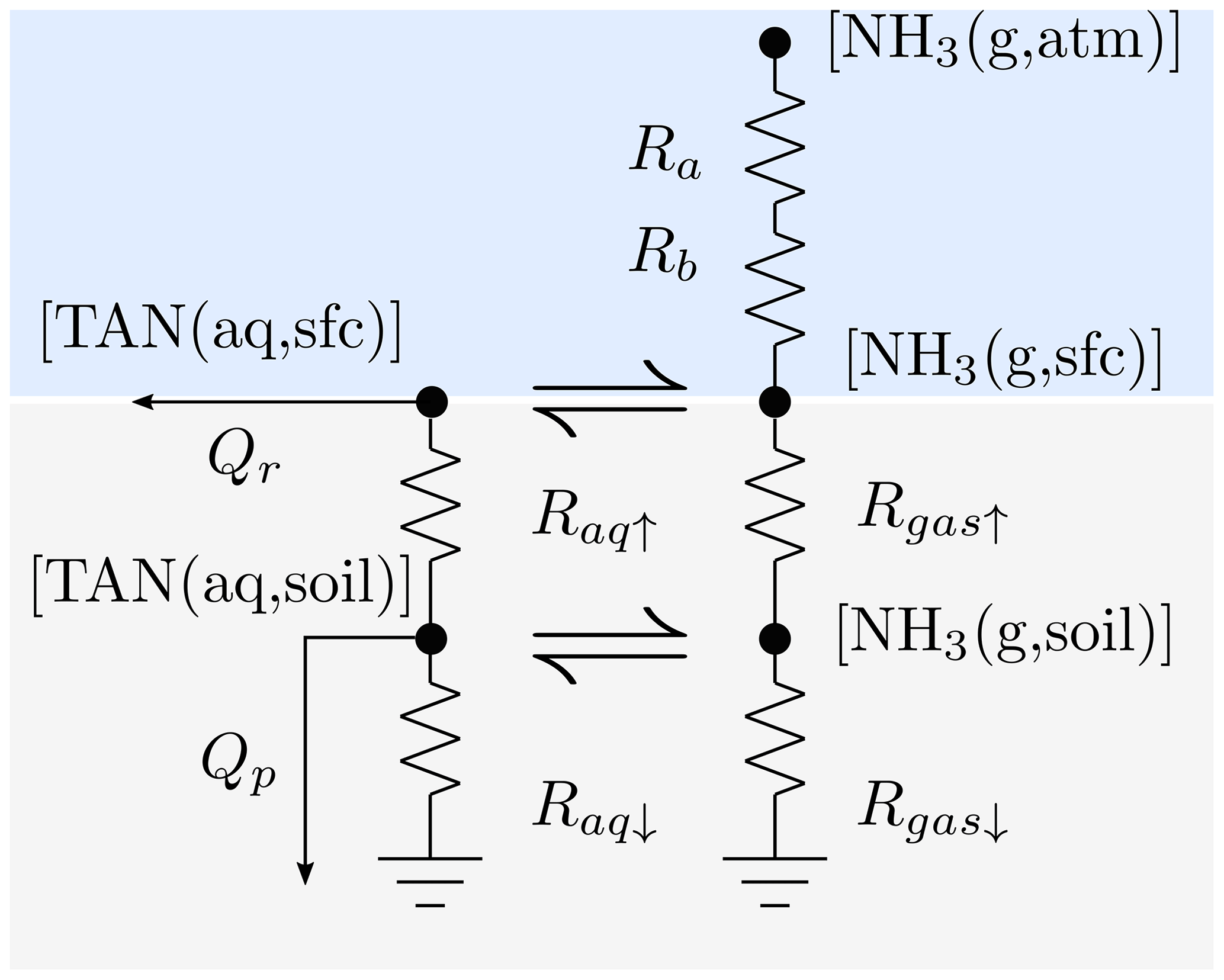
Figure 1A resistance scheme representing transport processes between the atmosphere, soil immediately below the surface, and the deeper soil. The aerodynamic and quasi-laminar layer resistances are denoted by Ra and Rb. Resistances controlling the diffusive transport upwards (↑) and downwards (↓) are denoted by Raq and Rgas for aqueous and gaseous phases; runoff and leaching fluxes are denoted by Qr and Qp. Phase equilibria are denoted with ⇌.
The exchange of NH3 between the soil surface and the atmospheric boundary layer is controlled by the aerodynamic and quasi-laminar resistances Ra and Rb. Below the soil surface, TAN is transported diffusively in the gas and aqueous phases or advectively in soil water. In FANv2, the dissolved TAN and urea can be leached either by surface runoff, representing lateral transport along the soil–air interface, or by percolating soil water, representing vertical transport within the soil column.
Following the resistance analogy, the surface flux of NH3 can be expressed using the NH3 concentration [NH3 (g,sfc)] at the soil–atmosphere interface,
where [NH3 (g,atm)] denotes the concentration at the atmospheric reference height consistent with Ra. The surface concentration [NH3 (g,sfc)] is a diagnostic variable determined by atmospheric concentration [NH3 (g,atm)] and the TAN concentration in soil.
The diffusive fluxes in soil are defined similarly to the atmospheric flux with resistances evaluated from the molecular diffusivities in soil:
where * denotes either the aqueous or gaseous phase, and the soil resistances are given by
The diffusion distance is taken as Δz∕2 and the molecular diffusivities D* are multiplied by the tortuosity factors ξ* of Millington and Quirk (1961) (Eqs. A6 and A7) to adjust for the soil porosity and water content. The aqueous-phase molecular diffusivity of ammonium (Eq. A8) is used for both ammonium and urea. The soil resistances for the downwards diffusion out of the topmost layer (marked with ↓ in Fig. 1) are evaluated similarly to Eq. (8), but the diffusion distance is set to 3 cm, which corresponds to the distance to the midpoint of the second soil layer in CLM5.
The aqueous-phase fluxes Qr (surface runoff) and Qp (subsurface leaching) are not diffusive (gradient-driven) but may nevertheless be included in the computations as
where qr (m s−1) is the surface runoff flux and qp the percolation flux of water at the bottom of the soil layer. An important difference between the modeled Qr and Qp is that the leaching flux Qp is evaluated from the mean concentration in the layer, while the runoff flux is evaluated from the concentration at the soil surface. Thus, Qr is moderated by the resistances and between the soil layer and the soil surface. The runoff water flux qroff is evaluated by CLM, while evaluation of qp depends on the manure or fertilizer type (Sect. 2.3 and S1.1 in the Supplement).
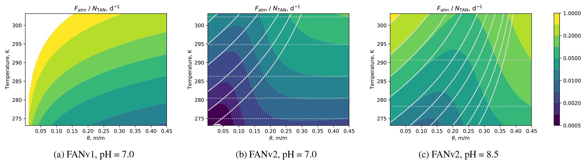
Figure 2The instantaneous volatilization flux normalized with the TAN pool, Fatm∕NTAN (d−1), as a function of temperature and volumetric soil moisture θ in FANv1 (a) in and FANv2 at pH = 7.0 (b) and pH = 8.5 (c). In all figures, θs=0.45, , and Qr=0. The contour lines correspond to the approximations at low (solid) and high (dotted lines) water content θ (Eqs. A21 and A22).
The atmospheric flux Fatm is determined by first solving the surface concentration [NH3 (g,srf)] as a function of the atmospheric and soil concentrations. Conservation of mass requires the aqueous and gaseous fluxes from the soil to the surface to be equal to the sum of the volatilization and runoff fluxes Fatm and Qr,
Using Eqs. (3) and (4) to calculate both the surface and soil concentrations, it is possible to solve for the aqueous and gaseous concentrations at the soil–atmosphere interface and subsequently for the fluxes Fatm and Qr. The expressions are given in Appendix A.
In summary, FANv2 largely inherits its parameterizations for chemical and biological processes from FANv1 but adds a more detailed description of the processes that transport TAN within the soil. FANv1 included leaching due to runoff (QR) but not due to the vertical movement of soil water (Qp). Furthermore, while diffusion of TAN in soils was included in FANv1, only downwards aqueous-phase diffusion deeper into the soil was considered, and adsorption of ammonium was neglected. Introducing these effects in FANv2 substantially changes the model's response to temperature and soil moisture.
The two-phase diffusion in FANv2, depicted in Fig. 1, allows TAN to be transported in either aqueous or gaseous phase within the soil layer. The relative importance of the two pathways depends on the equilibrium determined by and the resistances Raq and Rgas, which in turn depend on the water content trough the tortuosity ξ. This impacts how the volatilization flux Fatm responds to changes in , as shown in Fig. 2.
In contrast to FANv1, wherein Fatm is proportional to , the resistance model in FANv2 results in a nonlinear dependency on and θ. In the limiting cases of nearly saturated and nearly dry soil, the flux follows Monod expressions with respect to ,
where α is a function of θ, θs, and Kd; the expressions for α in each limiting case are given in Eqs. (A21) and (A22).
While both FANv1 and FANv2 predict the ammonia emission to increase with temperature (Fig. 2), the joint response to soil moisture and temperature differs between the versions: in FANv1, the flux always decreases towards higher θ, while in FANv2, the flux has a pH- and temperature-dependent minimum at ∼ 10 %–50 % saturation. In FANv2 the atmospheric flux (Fatm) at pH = 8.5 is 2–10 times higher than at pH = 7; however, the temperature sensitivity is higher at the lower pH. The higher pH (8.5) corresponds to the typical conditions following a urea application, as discussed in Sect. 2.4.4. FANv1 applies a 60 % reduction to the emission flux to account for the plant canopy capture and the soil resistance, which is not explicitly included in the formulation of FANv1. This reduction is applied to the flux shown for FANv1 in Fig. 2a, while no reduction is applied in FANv2, which evaluates NH3 volatilization from bare soil and excludes the effects of vegetation.
Several studies have shown that the presence of vegetation can significantly reduce volatilization losses (Black et al., 1989; Whitehead and Raistrick, 1992; Sommer et al., 1997), and thus FANv2 is likely to overestimate the NH3 emission under some conditions. However, for manure, the issue is not straightforward, since depending on the application method, the presence of vegetation may increase volatilization by intercepting the manure spread before it reaches the ground (Sommer et al., 1997). The canopy effect might be important for fertilizers applied later during the growing season, but as noted in Sect. 2.5.2, this practice is not simulated by CLM. For pastures, however, the simulations might be improved by including the effect of a canopy. Ideally, this would take into account interactions between grazing and plant growth.
Although the atmospheric NH3 concentration is included in Eq. (6), only gross fluxes are evaluated using FANv2 in this study, and [NH3 (g,atm)] is therefore set to zero in all simulations. This is consistent with the coupling to the atmospheric component of the CESM, whereby the dry deposition of ammonia is evaluated separately from emission. Although not evaluated here, the net NH3 exchange could be obtained by subtracting the dry deposition flux from the gross emission flux.
2.3 Upscaling from patch to grid scale
The model described in Sect. 2.2 can be used to evaluate the nitrogen fluxes from a horizontally homogeneous soil patch if the forcing variables such as soil temperature, moisture, pH, and the moisture fluxes qr and qp are known. However, some of the required parameters, such as pH and soil moisture, are sufficiently affected by the addition of manure or synthetic fertilizer to influence the volatilization fluxes. The perturbations in pH and moisture evolve as time passes since the N addition, and their magnitudes depend on the type of manure or fertilizer. As part of a global model, FANv2 needs to handle a heterogeneous distribution of soil patches in varying states with regard to nitrogen additions. The typical dimension of the soil patches might vary from less than 1 m (urine patches) to several kilometers (fertilized fields); in either case, the patches are small compared to ∼ 100 km horizontal resolution of current Earth system models.
This heterogeneity of patches is handled by assuming that the state of a nitrogen patch at a given time can be characterized by its age a, which we define as the time elapsed since the last N (fertilizer or manure) addition. We split each N (TAN or urea) pool into age classes and prescribe the perturbations in pH and moisture separately for each class. Thus, although the perturbations are prescribed, this approach allows using physically meaningful parameters to describe the differences between different types of N additions.
To formulate the approach mathematically, we distinguish between patch-scale nitrogen densities N (gN m−2 patch area) governed by Eq. (2) and grid-scale nitrogen densities n (gN m−2 grid cell area). The patches of a given type are divided into age classes i, each spanning a range of ages Δai. The total nitrogen pool is obtained by the summation over all the age classes. At each time step, the physical tendencies (Eq. 1) are first evaluated for each age class, then a fraction of N is transferred from the younger age classes to the older classes according to the age spans Δa. Details of this formulation are given in Sect. S1 in the Supplement.
The variation of soil pH and water content with patch age is embedded into the evaluation of Eq. (1) for each age class. In effect, adopting the generic model described in Sect. 2.2 for different sources of ammoniacal nitrogen becomes an exercise in defining the properties of a set of nitrogen pools as a function of age and the manure or synthetic fertilizer type. FANv2 considers two types of both manure and synthetic fertilizers, each described by a TAN pool with one to four age classes, resulting in the model structure shown schematically in Fig. 3. Additional nitrogen pools are needed for organic nitrogen in the case of manure and for unhydrolyzed urea in the case of urea fertilizer. An overview of the N pools and age classes is given in the next section; full details can be found in Sect. S2 in the Supplement.
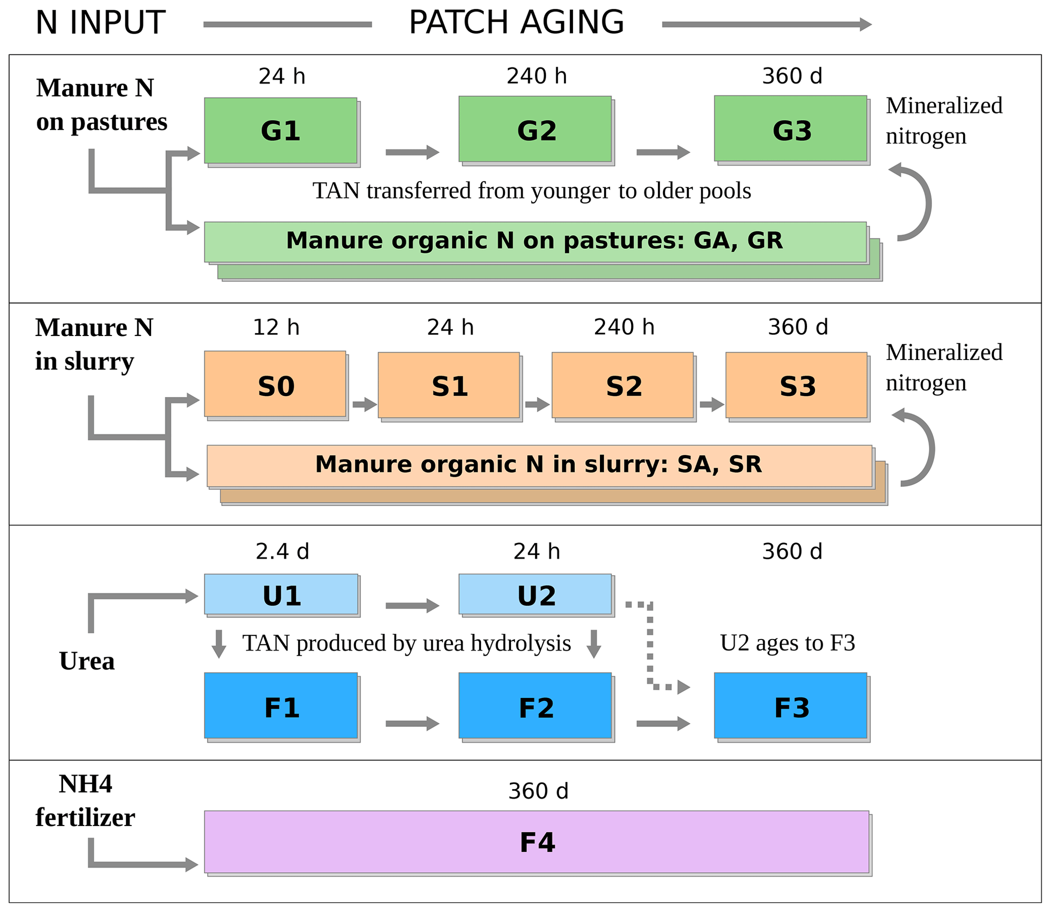
Figure 3Age-segregated nitrogen pools in FANv2 for manure TAN on pastures (G1–G3), manure TAN in slurry (S0–S3), urea N (U1–U2), TAN produced by urea hydrolysis (F1–F3), and from other fertilizers (F4). GA and GR as well as SA and SR represent available and resistant organic N on pastures and in slurry. The age extent Δa in days or hours is indicated for each age class.
2.4 Applications to specific agricultural processes
The parameterization of the soil processes and the setup of the age classes depend on the agricultural practice simulated. We simulate volatilization losses for four different processes: manure spreading, animals grazing in pastures, and synthetic fertilization modeled either as urea or a generic ammonium fertilizer.
2.4.1 Manure
FANv2 considers ammonia emissions separately for grazed pastures and for the application of stored manure. The emissions from manure application are simulated by the slurry sub-model (Sect. 2.4.3), while a simpler scheme focusing on urine patches is used for pastures (Sect. 2.4.2). The global distribution of manure N between pastures and managed manure is discussed in Sect. 2.5.
Regardless of the form, livestock manure contains nitrogen in the form of urea and more complex organic compounds. A typical fraction of urea nitrogen in dairy cattle manure is 60 % (Sommer and Hutchings, 2001); in FANv2, this fraction is used for all manure. The remaining manure N is split between organic N fractions with different mineralization rates as described in Sect. 2.2.
Decomposition of urea and other short-lived organic N forms is not evaluated explicitly within manure, as the urea contained within stored manure typically hydrolyzes during storage, and relatively short half-lives of less than 12 h have been observed for urea within urine patches in pastures (Sherlock and Goh, 1984). Similar to FANv1, FANv2 therefore assumes that all urea N in manure enters the soil as TAN.
Using slurry to represent manure management and spreading practices globally is a large simplification. However, the abundance of literature on ammonia volatilization from manure slurries supports the adoption of slurry as a “prototype” of global manure management practices in FANv2.
2.4.2 Grazed pastures
On pastures, manure N enters soil separately as urine and feces. In urine patches, the rapid hydrolysis of urea results in a local increase in soil pH, which exposes the newly formed ammoniacal N to rapid volatilization. Simultaneously, the volatilization loss is reduced by the infiltration and percolation of urine deeper into the soil. In contrast, fecal N remains on the soil surface, but with the slow mineralization of fecal N, ammonia is primarily emitted from the urine patches (Ryden et al., 1987).
Manure N excreted on pastures is represented by three age classes for TAN – G1, G2, and G3 – and the two organic N pools GA and GR (Fig. 3). The latter correspond to the available and resistant organic N fractions (see Sect. 2.2). The three TAN age classes describe the initial increase in soil pH within a urine patch (Vallis et al., 1982; Sherlock and Goh, 1984; Laubach et al., 2012) and the relaxation of soil water content from initial saturation back to the level of the surrounding soil.
At each time step, TAN is transferred from G1 to G2 and from G2 to G3 as the urine patches age. Class G1 represents patches less than 24 h old with a pH of 8.5, which decreases to 8.0 for the next 10 d, represented by G2, and returns to the base level in G3, which also receives the TAN mineralized from the organic pools GA and GR. The pH for G3 is taken from the Harmonized World Soil Database (HWSD; FAO and IIASA, 2009).
Urine is assumed to instantly infiltrate the soil and saturate the topmost soil layer simulated by FANv2. The soil moisture is assumed to return to the background level within the 24 h age span of G1, which results in a leaching flux dependent on the evaporation rate and the moisture differential between the saturated patch and the surrounding soil (Sect. S2.1 in the Supplement).
2.4.3 Slurry
Manure slurries consist of animal feces, urine, washing water, bedding, spilled feeds, drinking water, and possibly rainwater (Sommer and Hutchings, 2001). The amount of suspended solids in slurry is measured by the dry matter (DM) content (g DM g−1 slurry), which can vary due to different management practices from < 5 % up to about 20 %. Manure with a higher DM content can normally be handled as a solid (Lorimor et al., 2001). Several studies (Sommer and Olesen, 1991; Vandre et al., 1997; Misselbrook et al., 2005b) have shown a positive correlation between the DM content and NH3 volatilization. The suspended solids cause slurry to infiltrate soil slowly compared to water or urine, and consequently, large initial volatilization losses occur from broadcast slurry unless the slurry is mechanically incorporated into the soil (Pain et al., 1989; Van Der Molen et al., 1990b; Meisinger and Jokela, 2000; Sommer et al., 2003).
To capture this effect, FANv2 includes an additional age class (S0) representing soil patches with slurry partly remaining on the soil surface. Conceptually, S0 corresponds to the first phase of ammonia volatilization in slurry as described by Sommer et al. (2003). The age extent Δa of S0 defines the transition time to the second phase in which the slurry can be considered incorporated into the soil matrix. The rate of infiltration depends on hydraulic properties of both the slurry and soil (Misselbrook et al., 2005b; Sommer et al., 2006). However, this level of detail is not feasible to simulate in a global model, as the uncertainties related to slurry composition and application methods are too large. While a major simplification, we assume that the infiltration occurs in a fixed time defined by the age extent of S0.
The transport and transformation of N species in slurry are modeled following the overall approach described for soils in Sect. 2.2. However, due to the presence of slurry on the soil surface, the resistances in Eq. (7) for pool S0 need to be modified from those given in Eq. (8). Instead of the parallel resistances representing aqueous and gaseous diffusion (Fig. 1), the transport resistance within the slurry-covered soil is determined by two serial resistances (Fig. S1 in the Supplement), the upper representing the part of slurry remaining on the soil surface and the lower representing a saturated soil layer below. Expressions for the resistances are given in Sect. S2.2 in the Supplement.
The infiltration time, as needed to define Δa for S0, may be difficult to determine in practice, since a fraction of the water may be retained by the slurry solids for several days (Petersen and Andersen, 1996). Few observations are available to constrain Δa; Sommer and Jacobsen (1999) found 3 mm of pig slurry to infiltrate within 24 h of application, while Misselbrook et al. (2005a) reported 20 %–30 % of cattle slurry and up 80 % of pig slurry to infiltrate within 1 h. For the global simulations in this study, the infiltration time is set to 12 h; however, the effect of varying Δa of S0 will be investigated in Sect. 2.6.
The other nitrogen fluxes from S0 are evaluated with only minor modifications compared to the other pools. The slurry remaining on the soil surface is exposed to enhanced runoff losses (Jarvis et al., 1987; Smith et al., 2001); this is simulated by evaluating the runoff flux Qr for S0 directly from the bulk concentration of TAN instead of diagnosing the surface concentration as in Eq. (9).
The remaining slurry age classes S1 through S3, which represent slurry that has infiltrated into soil, are defined similarly to the classes G1 through G3 (grazed pastures) with minor adjustments to the pH based on the values given in Sommer and Olesen (1991), Bussink et al. (1994), and Sherlock et al. (2002) as described in Sect. S2.2 in the Supplement. Mineralization of organic N is handled analogously to the pastures using the N pools SA and SR, which feed the mineralized N into the oldest slurry TAN age class S3.
2.4.4 Synthetic fertilizers
In FANv2, the nitrogen applied in synthetic fertilizers is split between urea N, nitrate N, and ammonium N. Urea N is simulated in the greatest detail due to its significance in total NH3 emissions (e.g., Bouwman et al., 2002). Ammonium N includes the nitrogen in mineral fertilizers such as ammonium nitrate (AN), ammonium sulfate (AS), and ammonium phosphates. Volatilization losses from these fertilizers are normally low compared to urea (Whitehead and Raistrick, 1990; Sommer et al., 2004). An exception is ammonium bicarbonate (ABC), which is subject to similar volatilization losses as urea (Sommer et al., 2004; Bouwman et al., 2002). In FANv2, ABC is simply treated as urea. The nitrate N is not emitted as NH3 and therefore not tracked further in this study.
Three TAN age classes (F1, F2, and F3) and two urea age classes (U1 and U2) are used to evaluate the volatilization losses for urea fertilizers (Fig. 3). Formation of TAN in urea hydrolysis is evaluated explicitly, and the TAN formed in each age urea class (U1 and U2) is added to the corresponding TAN age class (F1 and F2). Fertilizer application is not assumed to change the soil moisture, but an increase in pH up to 8.5 is prescribed after Black et al. (1985), Whitehead and Raistrick (1990), and Sommer (2013). As in FANv1, urea hydrolysis is modeled as a first-order process with a time constant of 2.4 d (independent of soil temperature or moisture) adapted from the observations of Agehara and Warncke (2005).
As the fertilized patches age, TAN is transferred from F1 to F2 to F3, and urea N is transferred from U1 to U2. The transition between U1 and U2 matches the timescale for urea hydrolysis, and thus little urea remains unhydrolyzed by the end of U2. To avoid the need for a third urea pool, the remaining urea N in U2 is transferred directly to F3.
Other ammonium-based fertilizers do not form a strongly basic solution when applied on soil, which explains the smaller volatilization losses (Whitehead and Raistrick, 1990; Sommer et al., 2004). In FANv2, this is modeled by assigning the ammonium N to the single TAN pool F4 with pH taken from the HWSD database. Although this neglects the variations in soil chemistry between different types of fertilizers, the effect on total NH3 emissions is small due to the generally low volatilization losses. Since arable soils are frequently amended for pH, the pH for F4 is restricted between 5.5 and 7.5, which includes the preferred range for most field crops (Spurway, 1941).
2.5 Agricultural systems
The final step in the global application of FAN is linking the process model with datasets describing global agricultural practices. For synthetic fertilizers, this task is simplified by using the fertilization rates included in the CLM5 surface dataset (Lawrence et al., 2016), which is the dataset used within the Coupled Model Intercomparison Project Phase 6 (CMIP6). However, for manure, additional input data are needed to describe global patterns of livestock production, and additional parameterizations are needed to account for N losses in stored manure.
2.5.1 Livestock production systems and manure N
As described in Sect. 2.4.1, volatilization losses differ between manure excreted on pastures and manure spread mechanically. To distribute the manure N between the two pathways we follow Seré et al. (1996), Bouwman et al. (2005), and Beusen et al. (2008) and classify the global livestock into (i) pastoral and (ii) landless and mixed production systems. Pastoral systems are based on animal grazing in pastures, while in mixed and landless systems animals are typically confined to barns or feedlots. A significant fraction of NH3 emissions in mixed and landless systems occurs during storage and handling of manure (Beusen et al., 2008).
Since the currently available datasets of global manure N excretion do not differentiate between production systems, we compiled a new gridded dataset of yearly manure N excretion divided between these two systems. The global livestock density was obtained mainly from the Gridded Livestock of World (GLW) v2.01 dataset (Robinson et al., 2014), which includes the population densities of cattle, sheep, goats, pigs, and poultry for the year 2010. The density of buffalo was taken from an earlier version of the same dataset with the base year 2005. The animal densities were converted to nitrogen excretion rates using the coefficients recommended by the IPCC (2006). The excretion coefficients depend on the animal and the region and are listed in Sect. S3.1 in the Supplement. The total N excretion was 120 Tg N for 2010, which is within 10 % of the estimates of B. Zhang et al. (2017) (129 Tg N for 2010s), Potter et al. (2010) (128 Tg N for 2007), and Beusen et al. (2008) (112 Tg N for 2000). The N excretion was evaluated at 0.5∘ spatial resolution.
The manure N in each grid cell was divided between the pastoral and mixed–landless production systems as follows: all poultry and pig manure was assigned to mixed systems, while the ruminant manures (cattle, sheep, goats, and buffalo) were split between the two systems using the FAO Global Livestock Production Systems dataset (version 5; Robinson et al., 2011), which classifies the global land area into 12 livestock production categories. For each grid cell in the N excretion map, the fraction of ruminant manures attributed to pastoral systems was set equal to the area fraction of grassland-based (categories LGY, LGH, LGA, and LGT) production systems. The remainder, about 75 % of the manure N globally, was assigned to the mixed–landless production systems.
In pastoral systems, all manure is assumed to be excreted in pastures while grazing, while in mixed–landless systems, ruminants are assumed to graze seasonally. The fraction fgrz of ruminant manure excreted while grazing in mixed–landless production systems is evaluated dynamically as
where is the 10 d running average of daily minimum temperature and . The threshold temperature of +10 ∘C was used by Pinder et al. (2004) for modeling NH3 emissions from dairy farms in the US; the temperature threshold also explains some of the geographical variations in grazing reported in European survey data (Klimont and Brink, 2004, Sect. S4 in the Supplement), although regional differences are large. For pigs and poultry, fgrz is zero. Under these assumptions, about 60 % of the manure N in mixed–landless systems was assigned to barns in the 2010–2015 simulations, which is a similar to the estimate by Beusen et al. (2008).
The manure N remaining after subtracting the fraction fgrz is excreted in animal housings (e.g., barns) and then stored prior to being spread. The volatilization losses of ammonia in animal housings and manure stores cannot be described as a soil process; instead, we adopted a simpler mass flow scheme with empirical factors for the nitrogen losses based on the work of Gyldenkærne et al. (2005). The same parameterization was used by Paulot et al. (2014).
We assume that manure is removed from storage and applied to soil at a constant rate. While this assumption neglects seasonal patterns in manure spreading, manure management practices generally depend on local regulations, availability of workforce, and other factors that remain difficult to represent in a global model. Our approach furthermore assumes that the ammonia emissions at a given time in housings are proportional to the TAN produced in housings and that the amount of ammonia volatilized from storage is proportional to the TAN entering storage.
Under these assumptions, the NH3 emission from stores and housings is
where FTAN,excr is the rate of TAN excretion, fbarn is the fraction of TAN emitted in barns, and fstore is the fraction emitted in storage. The flux of TAN and organic N applied on soil is evaluated as
where Forg,excr is the organic N excreted in barns. The loss of organic nitrogen from housings and during storage is assumed to be negligible.
The fractions fbarn and fstore are evaluated using the parameterization of Gyldenkærne et al. (2005). In the parameterization, emissions from both housings and stores have the form
where T is the temperature in barns or stores, V is the effective ventilation rate, and a and b are constants. The values for a and b as well as the expressions of T and V are given by Gyldenkærne et al. (2005); the parameterization for naturally ventilated (open) barns are used for ruminants, and the values for mechanically ventilated (closed) barns are used for other livestock. The normalization constants C are set to 0.03 for open barns and 0.025 for closed barns and storage. The values were chosen to approximately reproduce the EMEP/EEA default emission factors (EEA, 2016) under European conditions.
Some of the stored manure may be used as fertilizer on croplands and some may be spread on grasslands. Volatilization losses from manure applied on crops and grasslands may differ due to differences in timing, vegetation cover, and method of manure application (Sommer and Hutchings, 2001). Since these details are not included in the model, for simplicity, our implementation applies all manure N on the natural soil column, which in the CLM sub-grid structure includes the grasslands plant functional type. The current CLM version does not include an explicit representation of pastures, and consequently, the natural soil column is also used to represent pastures in FANv2.
2.5.2 Synthetic fertilizers
In CLM5, the annual fertilizer application rate is prescribed depending on crop type, country, and year based on the Land-Use Harmonization 2 dataset (Lawrence et al., 2019; Hurtt et al., 2011). In the simulation, 79 Tg fertilizer N was applied in 2010, increasing to 87 Tg N for 2015.
The dataset does not specify the fertilizer type, and consequently, we used the country-level consumption statistics provided by the International Fertilizer Association (https://www.fertilizer.org, last access: 13 June 2018) to disaggregate the total fertilization rates into fractions of nitrate, urea, and ammonium N as discussed in Sect. 2.4.4. The N in ammonium nitrate, calcium ammonium nitrate, and compound fertilizers was split equally between ammonium and nitrate N; nitrogen solutions were assumed to contain 75 % of the nitrogen as ammonium and the remainder as nitrate. For China, the N reported under “other straight N” was attributed to ammonium bicarbonate following Bouwman et al. (2002) and, as described in Sect. 2.4.4, treated as urea.
In the CLM5 crop model, synthetic fertilizers are assumed to be applied exclusively on crop columns in a single application per growing season. Fertilization occurs during the leaf emergence phenological stage of the crop model and lasts for 20 d. The phenological stage is parameterized for each crop type based on thresholds for growing degree days and air temperature (Badger and Dirmeyer, 2015; Levis et al., 2018). As discussed in Lawrence et al. (2018), the 20 d fertilization window is inherited from earlier CLM versions, which were found to overestimate denitrification loss. However, for the purposes of FANv2, the 20 d window provides a useful representation of the variability of fertilization timing within a grid cell.
NH3 losses from fertilizers can be substantially reduced by placing or incorporating the fertilizer deeper into soil. Although mechanical incorporation is a standard practice for some crops and regions, global fertilization practices are not well characterized, and therefore we have not attempted to simulate the incorporation in detail. Instead, in FANv2 the effect of incorporation is simulated by reducing the fertilizer N available for volatilization by a constant 25 %. This assumes a typical 50 % reduction (Bouwman et al., 2002) applied to 50 % of the fertilizer N.
2.6 Model evaluation
The simulated volatilization rates using FANv2 were compared with the results from 21 studies published in peer-reviewed literature, with a total of 107 data points. Each comparison was based on a separate simulation, in which the CLM was first run in the single-point mode for the time and site of the experiment, and the simulated soil temperature, moisture, and other parameters were then used as the input for a stand-alone version of FANv2. The single-point CLM simulations were run in the satellite phenology mode and generally forced with the Global Soil Wetness Project Phase 3 (GSWP3) meteorological dataset (http://hydro.iis.u-tokyo.ac.jp/GSWP3, last access: 13 September 2020; Lawrence et al., 2019), which extends until 2014. The experiment of Bell et al. (2017) was performed in 2015 and simulated using the CRUNCEP dataset (Viovy, 2018).
The experimental studies were selected to provide a dataset covering volatilization from broadcast slurry applications, pastures, and synthetic fertilizers under various climate conditions.
Preference was given to measurements based on micrometeorological techniques. However, the enclosure-based measurements of Vallis et al. (1982) were included due to the scarcity of volatilization observations in warm (subtropical) conditions. Also, the measurements of Black et al. (1985) for ammonium sulfate, nitrate, and phosphates based on a similar enclosure method were included in order to better represent fertilizers other than urea. For the measurements of Black et al. (1985), the total atmospheric resistance (Ra+Rb) was replaced with
where A is the soil area covered by the measurement chamber and Q is the air flux (m3 s−1) through the chamber. In the measurements of Vallis et al. (1982), the flow rate was adjusted to follow the near-surface wind speed, and the Ra and Rb from CLM were used as for all other experiments. Whenever several replicate measurements were reported for the same time and site, only the averaged losses were compared to the model.
Generally, the experiments represented the local ambient conditions. The only exception was the experiment of Holcomb et al. (2011), which evaluates the effect of varying irrigation rates on NH3 emissions. The irrigation was introduced to the CLM simulations as precipitation; a separate CLM simulation was run for each irrigation experiment. The experiments on pastures include both simulated urine patches and pastures with grazing livestock. For fertilizers, only experiments using surface application were included, and the 25 % reduction due to incorporation (Sect. 2.5.2) was therefore not used. The timing and duration of the N applications were replicated in the simulations as reported for each study. Since FANv2 is linear with respect to the absolute N input (for a given meteorological forcing), we did not consider the effect of the N application rate, but instead evaluate only fractional NH3 emissions normalized by the amount of N applied.
The simulated volatilization rates were unavoidably affected by the uncertainties in the variables simulated by the CLM and in the meteorological forcing. However, most of the experimental studies did not characterize the atmospheric and soil conditions sufficiently to provide input for the FANv2 model. Furthermore, running FAN in combination with the CLM can be expected to give a more realistic assessment of the model's performance in its intended application.
Some parts of the world are underrepresented in the available literature on micrometeorological NH3 flux measurements. Our dataset contains no measurements in India or Africa and only one study in China. Including data covering a wider range of measurement techniques, such as static or dynamic chambers or wind tunnels, could widen the geographical coverage – for example, a number of studies based on enclosure or tracer techniques would be available for China (L. Zhang et al., 2018). However, the effects of heterogeneity in the measurement techniques would need to be assessed carefully, since systematic differences (Bouwman et al., 2002; Sintermann et al., 2012; Harper, 2005) have been found between the volatilization losses measured using different techniques.
2.7 Setup for global simulations
The global ammonia emissions analyzed below (Sect. 3.2) are based on a 6-year simulation using the Community Earth System Model (CESM), which couples the CLM with the Community Atmospheric Model (CAM). As part of CLM, the FANv2 ammonia emissions were evaluated interactively at each time step using the meteorological forcing from the atmospheric model. The simulation covered the years from 2010 to 2015. The year 2009 was run as spin-up.
The model was run on a global longitude–latitude grid with 2.5∘ × 1.9∘ spacing and a 30 min coupling time step. CAM version 5.4 was used, configured with the CAM4 physics package and run in the “offline” mode (Lamarque et al., 2012) with the atmospheric dynamics prescribed by the MERRA reanalysis fields.
In addition to the 6-year simulations coupled to CAM, a set of 2-year (2010 and 2011) simulations was run to evaluate the model's parameter sensitivity. To reduce the computational burden, these simulations were run in land-only mode with the atmospheric forcing given by the GSWP3 dataset.
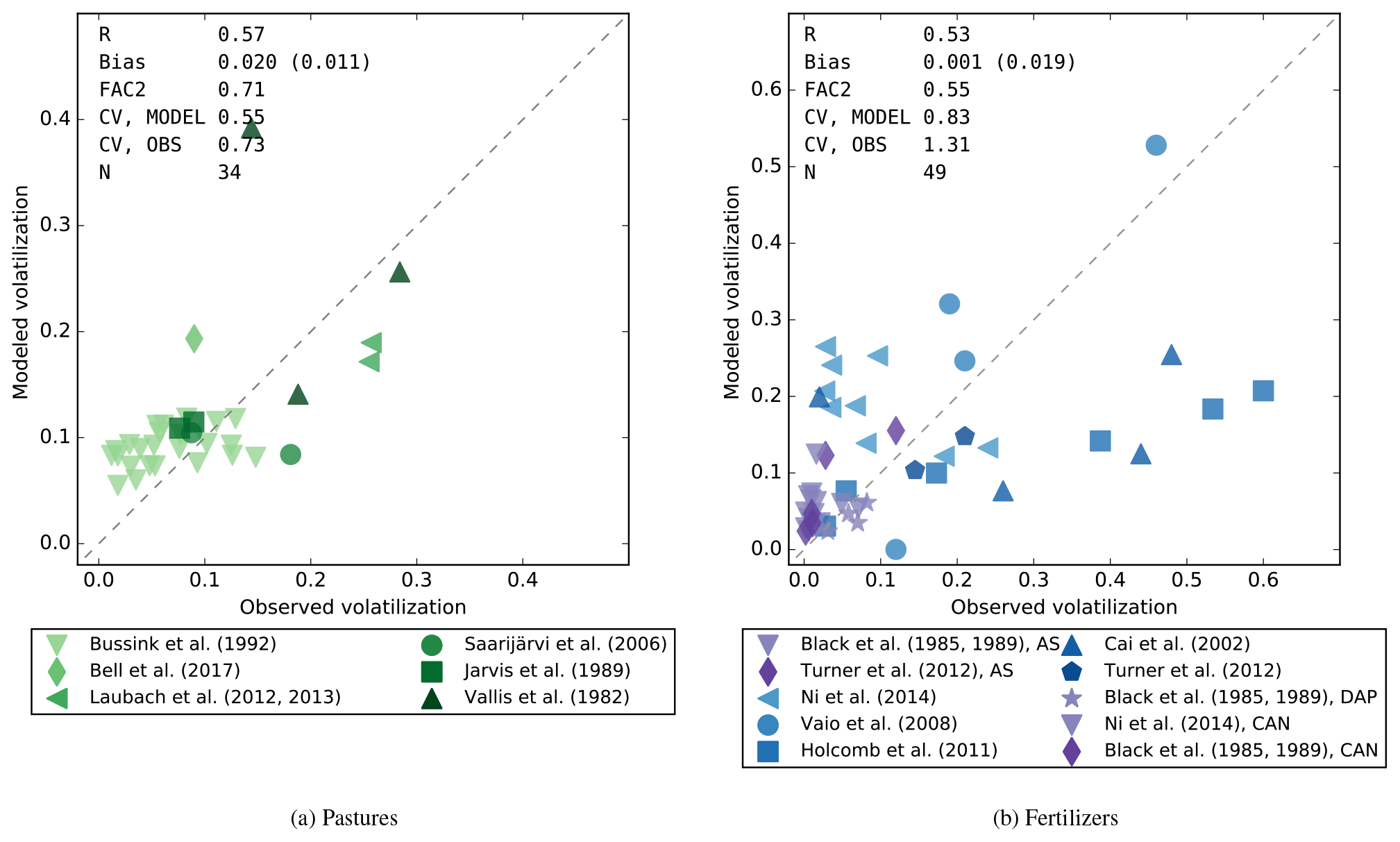
Figure 4Modeled volatilization losses (fraction relative to the applied N) compared with field observations for urine patches (a) and for synthetic fertilizers (b). The data for fertilizers include urea, shown with blue markers, diammonium phosphate (DAP), ammonium sulfate (AS), and calcium ammonium nitrate (CAN), shown with purple markers. Abbreviations used for statistical indicators: R – Pearson's correlation coefficient, FAC2 – fraction of values within a factor of 2, CV – coefficient of variation, N – number of points.
3.1 Evaluation against field measurements
The simulated volatilization losses were evaluated against data from experimental studies, which consist of one or more experiments typically spanning a period of several weeks. The observations are therefore local in both space and time, which makes them challenging to reproduce with a model intended for continental or global scales. Difficulties may arise, particularly due to the emissions' complex response to soil moisture (Sect. 2.2), which could be affected by local-scale orography and drainage conditions as well as unresolved precipitation patterns. The evaluation presented here therefore focuses on the model's ability to mechanistically reproduce the differences in the volatilization rates from different types of fertilizers and manure.
A comparison of the modeled and measured volatilization rates (cumulative emission flux divided by the N input) is shown for grazed pastures in Fig. 4a. The correlation between the model and measurements was R=0.57. FANv2 captures the tendency towards higher volatilization at the warmer sites (Vallis et al., 1982; Laubach et al., 2012, 2013) reaching 30 %, although one of the measurements of Vallis et al. (1982) is overestimated by the model. This measurement had the highest air and soil temperature (up to +36 ∘C) among the three measurements in Vallis et al. (1982) yet the lowest volatilization loss.
The measurements of Bussink (1992) and Jarvis et al. (1989) evaluate volatilization losses on pastures under varying N fertilization rates. Since the effect of fertilization prior to grazing cannot be simulated by FANv2, the replicates with different N fertilization were averaged when possible. However, this was not possible with most of the data in Bussink (1992) because the different treatments were applied at different times, which likely explains why the model did not reproduce most of the variability within the Bussink (1992) dataset. Nevertheless, the average losses taken over the Bussink (1992) data were reproduced reasonably well.
Similar to pastures, in the comparison for synthetic fertilizers (Fig. 4b) the model has a small average bias (< 1 % of the applied N), although the correlation between the model and the data is moderate (R = 0.53). The contrast between urea (blue markers) and other fertilizers (purple markers) is captured. Also, the decrease in volatilization with increasing irrigation in the measurements of Holcomb et al. (2011) is reproduced, although the simulated volatilization is underestimated in the lightly irrigated treatments, with measured volatilization losses up to 60 %.
Finally, Fig. 5 compares the simulated volatilization losses with observations for surface-applied slurry. In Fig. 5a, the model was run with a constant application rate of 50 m3 ha−1 and infiltration time (Δa for S0, Sect. 2.4.3) τinfl=12 h, which are the default values chosen for the global simulations. In this configuration, the model captures the average volatilization losses, which are higher than for urea or pastures, but the observations of Spirig et al. (2010) and Sintermann et al. (2011) are strongly overestimated, and the model is not significantly correlated with observations (R=0.27, p=0.19). The modest agreement with the observations suggests that a significant fraction of the variation might not be related to the variations in ambient conditions.
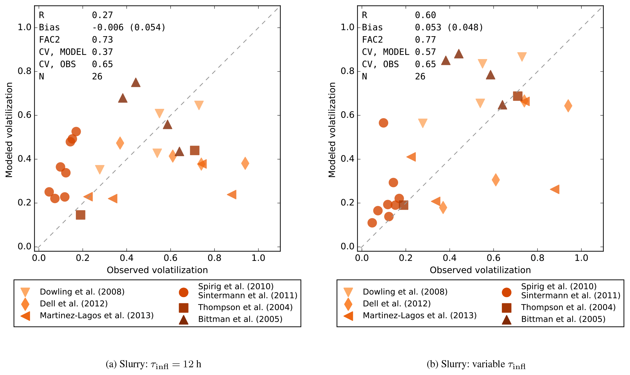
Figure 5Modeled volatilization losses compared with field observations for slurry. (a) Results with 12 h infiltration time and no adjustment for application rate. (b) Results using reported application rates and infiltration times adjusted based on dry matter content. Abbreviations used are as in Fig. 4.
The experiments of Spirig et al. (2010) and Sintermann et al. (2011) were carried out using mixtures of cattle and swine slurries with DM contents mostly between 1 and 3 %, while the other studies include slurries with up to 12 % DM. Similarly, the application rate varied from 30 up to 100 m3 ha−1 (3–10 mm) in the various studies. While the application rate is an input parameter for FANv2 as noted in Sect. 2.4.3, the DM content is not directly related to any of the model parameters. However, the DM content is related to the infiltration rate of slurry (Misselbrook et al., 2005b; Sommer et al., 2006), and by assuming a simple relation between the DM content and the infiltration rate, it was possible to tune the model to provide a better match to the observations.
The comparison in Fig. 5b is obtained by setting the initial slurry depth d0 equal to the reported application rate and setting the infiltration time , where the slurry infiltration rate qs decreases linearly from 2.5 mm h−1 at DM ≤ 1 % to 0.125 mm h−1 at DM ≥ 4 %. This adjustment effectively causes the model to treat the dilute slurries similarly to urine. When adjusted for the DM content and application rate, the modeled volatilization losses are significantly correlated with the observations (R=0.60, p<0.01). Thus, for the datasets included in this study, the variations of DM and application rate indeed appear to explain a considerable fraction of the variation in the observations. The data of Spirig et al. (2010), Sintermann et al. (2011), and Thompson and Meisinger (2004) are especially well reproduced after adjusting for slurry characteristics. The slurry characteristics also appear to explain the variations between measurements of Dell et al. (2012), although the model tends to underestimate the volatilization loss in these measurements.
Parameters like DM content and application rate are not available for global simulations. Similar to the case for slurry, the evaluations for pastures and fertilizers are likely to be affected by insufficiently known parameters, such as the urine volume d0 and the layer thickness Δz, which for fertilizers can be interpreted as the depth of application. The model sensitivity to these parameters is discussed with regard to the global simulations in Sect. 3.3. However, globally, even more substantial variations may arise from different application methods. When applied on arable land, both fertilizers and manure are frequently incorporated mechanically, which results in a large reduction of volatilization losses (Sommer, 2013; Pan et al., 2016). Further uncertainty arises from various types of manure, such as deep litter or farmyard manure, which are currently not implemented in the model. With sufficient observational data, these practices could also be included in the model.

Figure 6Simulated ammonia emissions () from urea (a) and other synthetic fertilizers (b) averaged over 2010–2015. Note the different color scales.
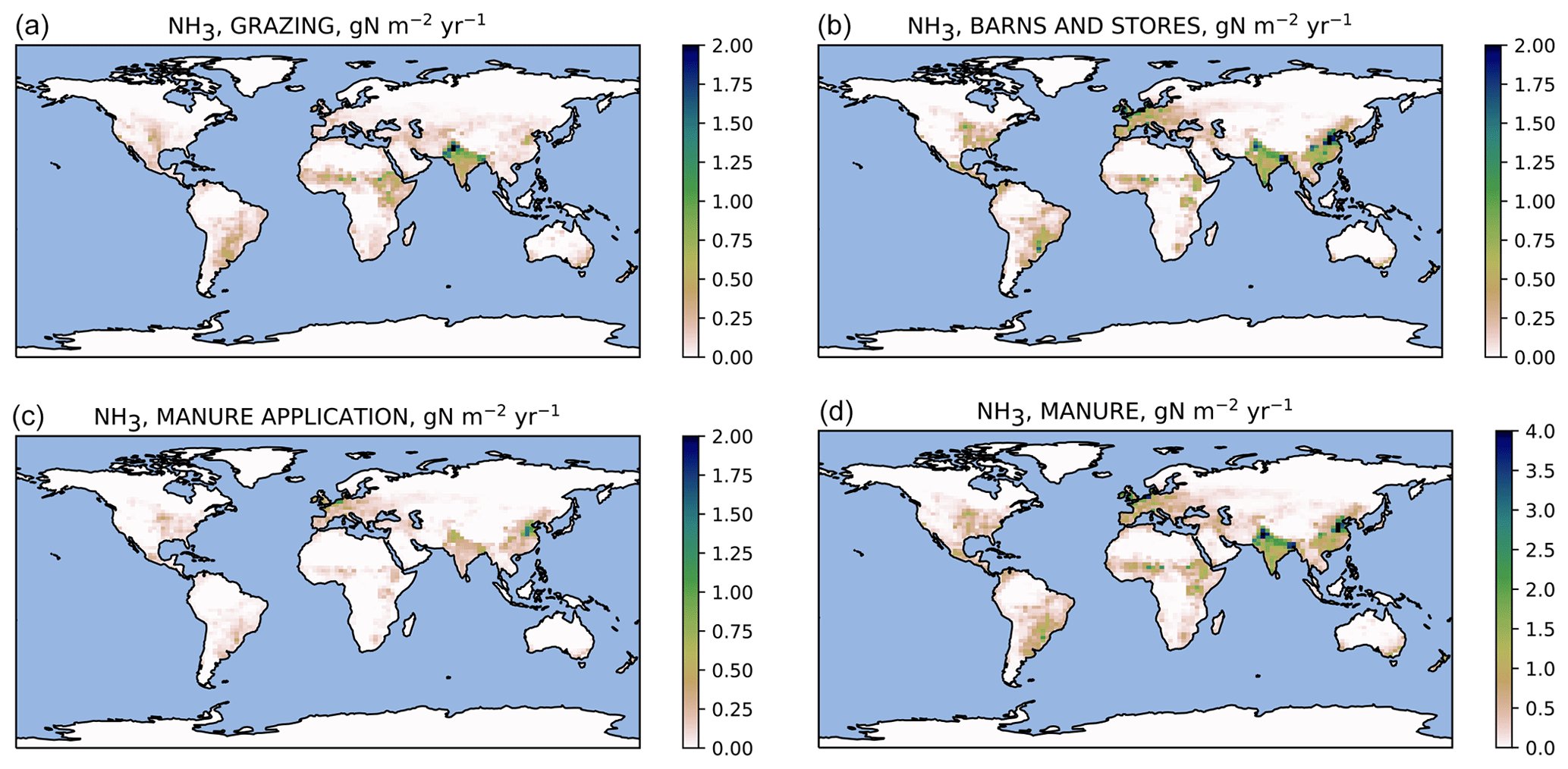
Figure 7Simulated ammonia emissions () from manure: pastures (a), barns and storage (b), manure application (c), and total from manure (d) averaged over 2010–2015. Note the different color scale for panel (d).
If the data from all experiments are pooled together and the default parameters are assumed for slurry, the modeled volatilization loss was within factor of 2 of the observed in 64 % of the cases, and the model reproduces the observed losses with R=0.66 and a mean bias of ∼ 1 % for the applied N. Thus, the model captures variations in volatilization losses associated with different forms of nitrogen application with a small overall bias. The modeled coefficient of variation was for all categories lower than observed, as could be expected in the absence of site-specific adaptations.
3.2 Global NH3 emissions
The simulated global agricultural ammonia emissions for 2010–2015 were 48 Tg N yr−1, consisting of 37 Tg N from manure and 11 Tg N from the use of synthetic fertilizers. The manure emissions include 12 Tg N from grazed pastures, 18 Tg N from barns and stores, and 6.5 Tg N from manure application. The fertilizer emissions consist of 8.1 Tg N from urea and ammonium bicarbonate and 2.9 Tg N from all other synthetic fertilizers.
Geographically, the highest emissions for urea and other fertilizers (Fig. 6) occur in China and India. The highest emissions from manure (Fig. 7) partly coincide with those from fertilizers; however, significant emissions also occur in regions such as equatorial Africa and South America where fertilizer usage is low. The highest relative volatilization losses for both fertilizers and manure (Figs. 8 and 9) are associated with regions with warm and often arid climates. The losses in equatorial regions are relatively low due to high precipitation, with the exception of losses in barns and manure stores from which emissions are assumed to be unaffected by rain.

Figure 8Fraction of fertilizer N lost due to volatilization averaged for 2010–2015: urea (a) and other synthetic fertilizers (b).
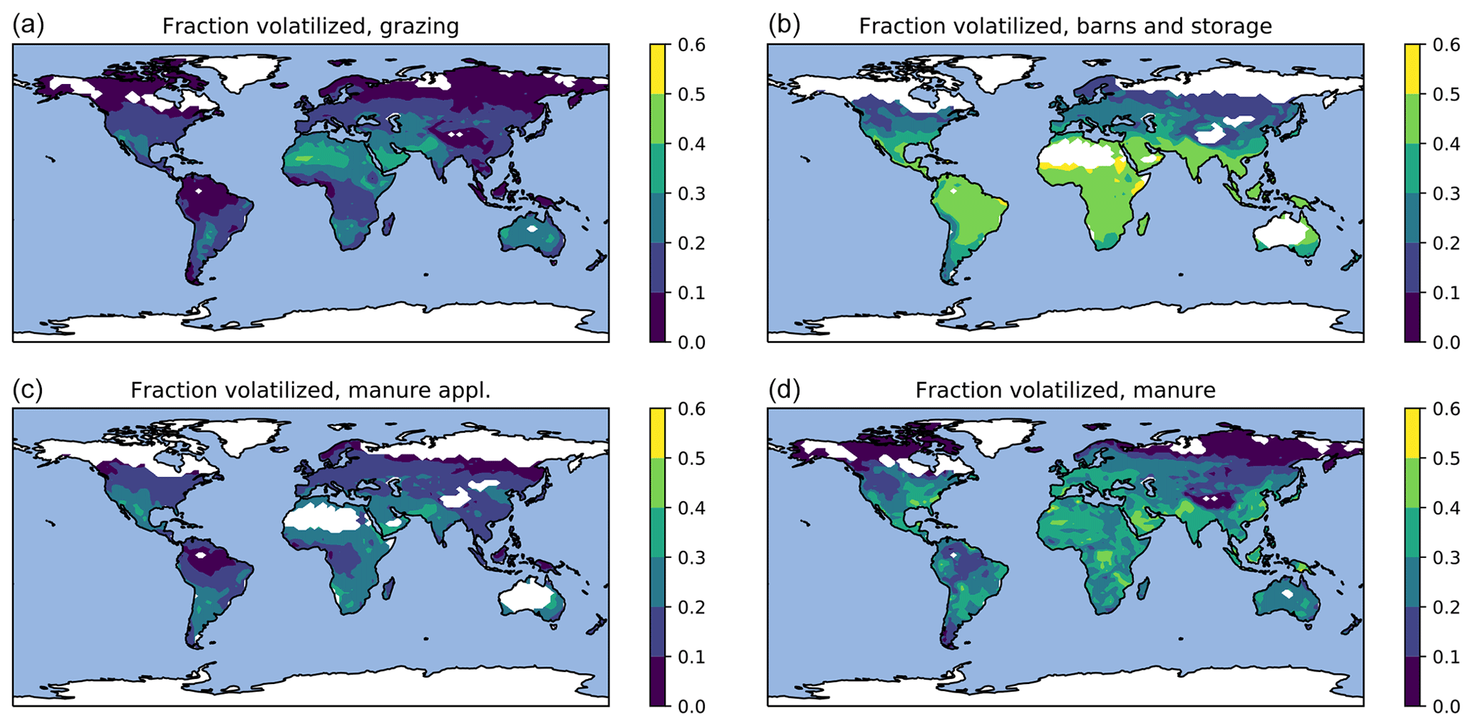
Figure 9Fraction of manure N lost due to volatilization averaged for 2010–2015: grazing (a), barns and storage (b), manure application (c), and all manure (d).
The volatilization losses are shown as fractions of the N inputs in Table 1. The losses from manure application are shown with respect to both applied TAN and total (organic and ammoniacal) nitrogen. Since the higher losses in housings and storage result in lower TAN fractions in the applied manure, normalizing the losses by the TAN applied reveals a much higher regional variability than is apparent from the losses calculated with respect to total N. It should be noted that the fraction normalized by the applied TAN is not exactly equal to the real fraction of TAN volatilized, since some of the emissions actually originate from the organic fraction (Sect. 2.2).
Table 1Global and regional averages of volatilization losses in agricultural activities. The losses are given as fractions of total (organic and inorganic) manure or fertilizer nitrogen unless stated otherwise. The total volatilization loss for manure includes emissions from all individual processes normalized by the total manure N produced in the region. The average loss for synthetic fertilizers consists of emissions from urea and other fertilizers normalized by the total fertilizer N applied.
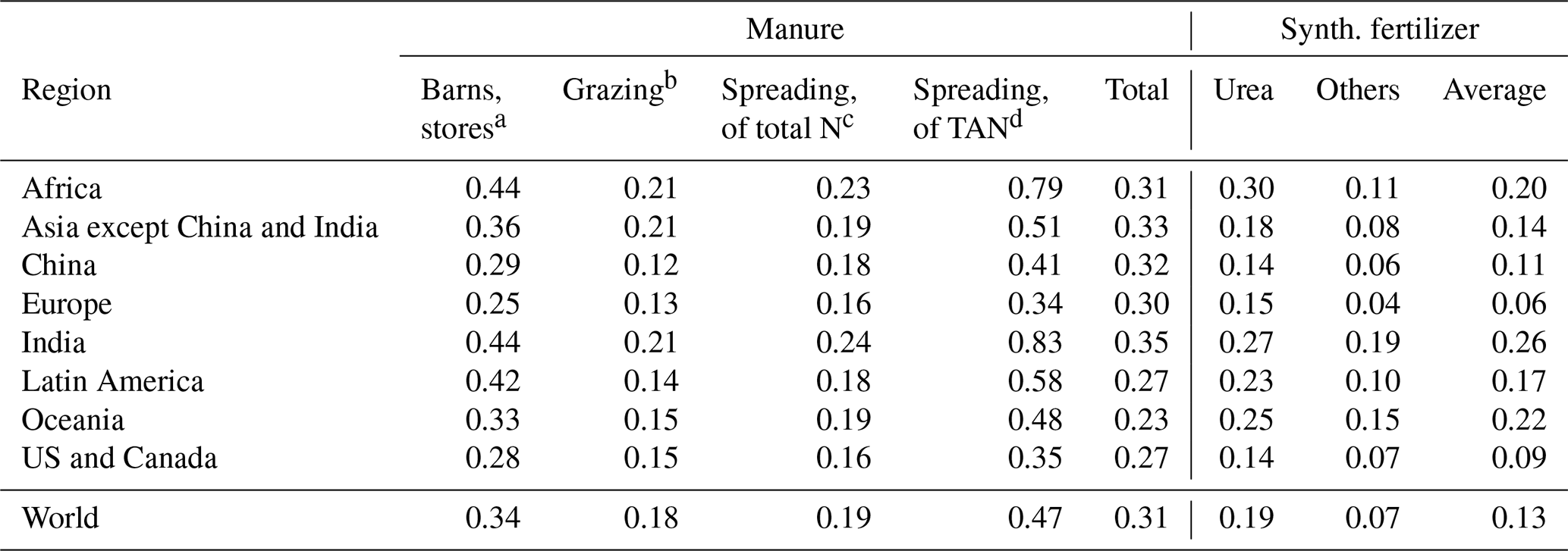
a As fraction of N excreted in barns;
b as fraction of N excreted while grazing;
c as fraction of N remaining after losses in storage and housings;
d as fraction of TAN remaining after losses in storage and housings.
The predominant processes limiting the volatilization loss were diffusion and leaching of TAN deeper into the soil; for both manure and fertilizers, about 55 % of the input N was removed from the FANv2 pools via this pathway (data not shown). The role of nitrification was generally smaller: about 12 % (15 %) of the manure (fertilizer) N was nitrified within FANv2. The loss due to surface runoff as or urea was 1.7 % for fertilizer and 0.8 % for manure N. Note that the runoff loss evaluated by FANv2 does not include subsurface leaching or any runoff or leaching of nitrate N.
Figure 10 compares the FANv2 emissions regionally and globally with version 4.3.2 of the EDGAR emission inventory (Crippa et al., 2018). Globally, the FANv2 emissions (48 Tg N yr−1) are about 17 % greater than the EDGAR emissions (41 Tg N yr−1 from the agricultural sector). The regional comparison shows that the difference is largely due to emissions in Africa, India, and Latin America, while for China, the EDGAR emissions are about 50 % higher than FANv2. For Europe and North America, FANv2 and EDGAR are in good agreement.
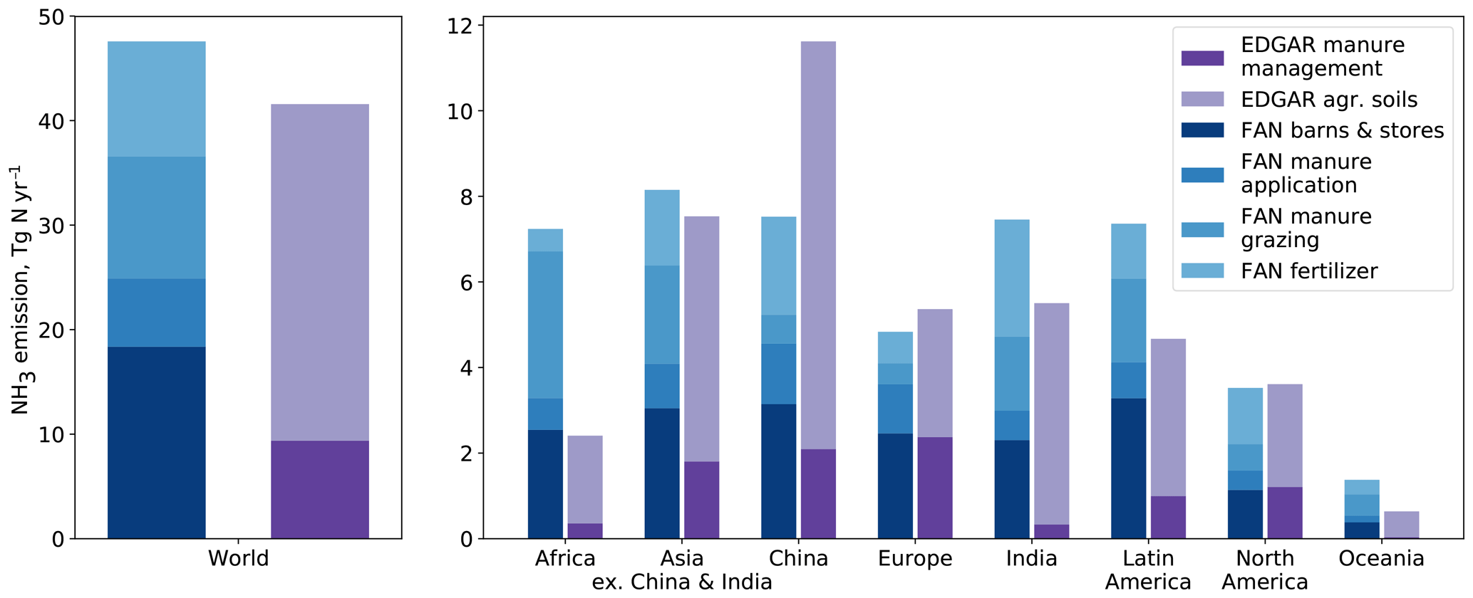
Figure 10Global and regional ammonia emissions from agricultural sources in FANv2 (for the years 2010–2015) and EDGAR v4.3.2 (for 2010; Crippa et al., 2018; Tg N yr−1). The EDGAR manure management emissions correspond to barns and stores in FANv2.
The EDGAR emissions are split into two reporting categories: “manure management”, which includes emissions from animal housings and stored manure, and “agricultural soils”, which includes emissions from soils (from both manure or synthetic fertilizer application and grazing). As seen in Fig. 10, the split between the categories is similar for FANv2 and EDGAR for Europe and North America, where the total emissions are also similar. Conversely, the regions where FANv2 and EDGAR differ most also have large differences in the contributions from the two emission categories. In particular, a significant fraction of manure in Africa, India, and Latin America is attributed to mixed production systems in FANv2. This leads to large emissions from housings and manure stores in FANv2, while in EDGAR, manure management contributes only minimally to the emissions in these regions.
Table 2 compares FANv2 with additional regional and global emission inventories. FANv2 and EDGAR agree within 10 % with the national emission inventories for the US and Canada (EPA/EC); also, the split between manure and synthetic fertilizers is similar in FANv2 and the EPA/EC inventories. For Europe, the FANv2 emissions are in agreement with EDGAR but 23 % higher than those reported in the EMEP emission inventory, mainly due to larger emissions in the “agricultural soils” category.
Table 2Simulated NH3 emissions by region averaged for the years 2010–2015 and compared with existing inventories. The total emission is equal to manure management + agricultural soils or total manure + synthetic fertilizer. For FANv2, manure management emissions are equal to the emissions from barns and storage.
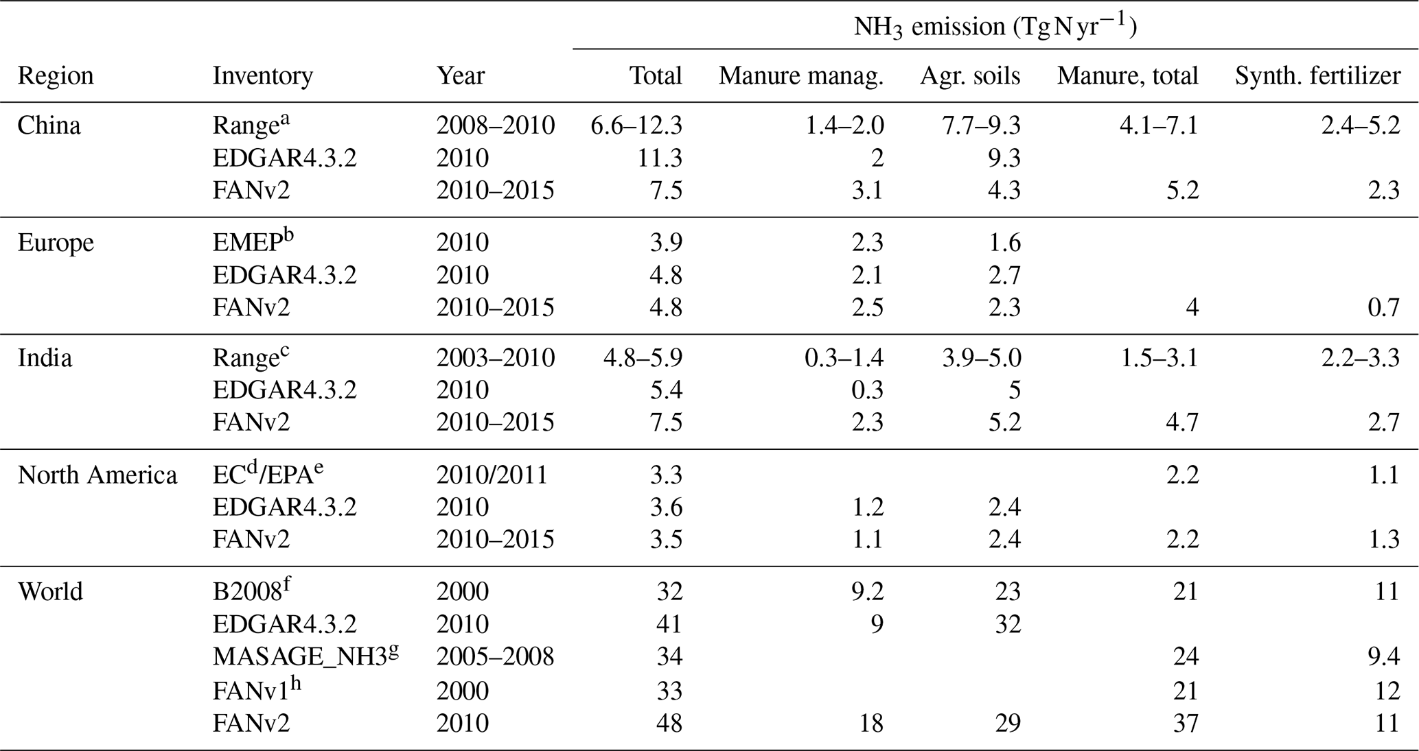
a Kang et al. (2016); Xu et al. (2018); Kurokawa et al. (2013); L. Zhang et al. (2018); X. Zhang et al. (2017).
b EMEP/CEIP 2018, https://www.ceip.at/webdab-emission-database/emissions-as-used-in-emep-models (last access: 13 September 2020).
c Aneja et al. (2012); Kurokawa et al. (2013); Xu et al. (2018).
d https://pollution-waste.canada.ca/air-emission-inventory (last access: 5 July 2018)
e https://www.epa.gov/air-emissions-inventories/2011-national-emissions-inventory-nei-data (last access: 5 April 2018)
f Beusen et al. (2008).
g Paulot et al. (2014).
h Riddick et al. (2016).
Ammonia emissions in China have been studied intensively, and only studies with the base year 2008 or later are included in Table 2. The FANv2 emissions (7.5 Tg N) are within the range of published estimates, albeit on the lower end, mainly due to lower emissions from fertilizer application. In contrast, the FANv2 emissions for India are about 25 %–50 % higher than in previously published global and regional inventories, mainly due to higher emissions from manure management and grazing.
We are not aware of regional emission inventories covering all of South and Central America, but national inventories have been compiled for Chile (Muñoz et al., 2016, livestock only) and Argentina (Castesana et al., 2018). For Chile, the estimate of Muñoz et al. (2016) of 57 Gg N (69 Gg NH3) from livestock for 2013 is comparable to the FANv2-simulated emission of 70 Gg N for 2010–2015. For Argentina, Castesana et al. (2018) estimated annual emissions of 139 Gg N (169 Gg NH3) from manure and 119 Gg N (145 Gg NH3) from mineral fertilizers in 2010–2012 – far less than the corresponding FAN emissions of 760 and 260 Gg N. The higher fertilizer emissions in Argentina simulated by FANv2 are largely explained by higher fertilizer use in the CLM dataset (1400 Gg N compared to 400–900 Gg N reported by Castesana et al., 2018). The fertilizer use of Castesana et al. (2018) is consistent with the IFA statistics for 2010–2015. However, the difference in manure NH3 emissions appears to be caused by a much higher emission factor implied by the FANv2 simulation.
In Africa, the FANv2 emissions from grazing alone (3.4 Tg N) exceed the total NH3 emissions (2.4 Tg N) reported in the EDGAR inventory. Comprehensive regional NH3 emission inventories for Africa are not available. However, assuming a fixed 30 % volatilization loss, Delon et al. (2010) estimated 1.5 ± 0.8 Tg N yr−1 emitted within the Sahel region, which is consistent with the FANv2 emissions of 1.2 Tg N yr−1 for the same region.
Compared to FANv1, the total emissions in FANv2 are about 45 % higher. This difference is mainly caused by the volatilization loss from manure, which is 31 % of manure N in FANv2 but only 17 % in FANv1. As a consequence, the total emissions in FANv1 were relatively low, especially for China (5.2 Tg N) and Europe (1.9 Tg N), and for these regions, the emissions simulated by FANv2 (Table 2) are closer to the available regional inventories. The volatilization rates for synthetic fertilizers differ between FANv1 and FANv2, albeit less drastically: FANv1 treated all fertilizers as urea, resulting in a higher total volatilization rate (19 %) for synthetic fertilizers than FANv2 (13 %) – however, the mean volatilization rate for urea in FANv2 is 19 %, which is similar to FANv1.
The FANv1 emissions include a fixed 60 % reduction to account for canopy uptake of ammonia. However, the formulation in FANv1 did not include a soil resistance, which in FANv2 largely controls the emission flux. The 60 % reduction in FANv1 therefore has to be understood to include the effects of both soil resistance and the canopy uptake, which makes a quantitative comparison between the two model versions difficult. In addition to the reduction factor, a major difference between FANv1 and FANv2 is that FANv1 does not differentiate between emissions in storage and housing, manure application, and grazing. This may explain why the difference in the volatilization rates is larger for manure than for synthetic fertilizers.
3.3 Sensitivity to model parameters
As a process model FANv2 uses a number of poorly constrained parameters. A set of 2-year simulations was run to investigate the model's sensitivity to its parameters as described Sect. S5 in the Supplement. The sensitivity experiments used a different meteorological forcing than the main simulations (GSWP3 instead of the CAM simulation), which increased the global emissions for 2010–2011 by 2 %. On a global level, the model therefore appears fairly robust with regard to the meteorological input.
Overall, the model was also relatively insensitive (<10 % change in global emission, ∼ 0.1 %–0.2 % per percent change in parameter) to parameters affecting any individual process, such as slurry infiltration, urea hydrolysis, or the timing of fertilization (Table S2 in the Supplement). The parameters with a more systematic effect, and therefore higher sensitivity, included the thickness of the model layer (Δz), the adsorption parameter Kd, the manure TAN fraction fTAN, and the maximum grazing fraction (, Sect. 2.5.1). A 10 % change in the TAN fraction or the grazing fraction changes the global manure NH3 emission by 3–4 and 8 %, respectively.
The sensitivity for both Δz and Kd was higher for fertilizers than for manure. Varying Kd between 0 and 10 times the default changed the manure emissions by −29 % to +11 %, while for fertilizers, the range was −55 % to +30 %. For manure, varying Δz (by default 2 cm) between 4 and 1 cm changed the emission by −19 % to +6 %. However, for fertilizers, doubling the Δz to 4 cm reduced the emissions by 52 %, while halving Δz increased the emissions by 41 %. This response is roughly comparable with the observed effect of incorporating urea into soil as evaluated in the literature survey of Rochette et al. (2013); in the polynomial fit of Rochette et al. (2013) increasing the incorporation depth from 2 to 4 cm reduces emissions by ∼ 40 %, while reducing the depth to 1 cm increases emissions by ∼ 23 %.
3.4 Sensitivity to mean temperature and precipitation
The characterization of ammonia emission rates on climate and interannual timescales is important for climate, pollution, ecological, and agricultural applications, but it remains poorly quantified. Based on a synthesis of empirical and theoretical considerations, Sutton et al. (2013) estimated the ammonia emission from fertilizers and manure to increase by 3 %–7 % for each 1 K increase in mean temperature. Consistent with the analysis of Sect. 2.2, Sutton et al. (2013) note that the sensitivity observed empirically was typically lower than implied by the thermodynamic partitioning between gaseous and dissolved NH3 (Eq. 3).
Although only present-day emissions were evaluated in this study, the simulated geographical variation in volatilization rates can be used to derive a crude estimate of how NH3 emissions respond to changes in mean temperature and rainfall. The response was evaluated using the linear regression approach described in Sect. S6 in the Supplement. In brief, we first categorize the model grid cells by yearly rainfall, then for each category linearly regress the average volatilization rate (NH3 emission divided by N application) with the mean temperature, and finally apply the regression slope weighted by the N application in each category to obtain the average temperature sensitivity for manure, urea, and other fertilizers.
The temperature sensitivity (Table 3) was higher for fertilizers (6 % K−1–10 % K−1) than for manure (2 % K−1). The overall temperature sensitivity of ammonia emissions from all sources was ∼ 3 % K−1, which is at the lower end of the range given by Sutton et al. (2013). However, the FANv2 estimate implicitly includes changes in agricultural practices due to the effect of increased grazing and earlier planting dates in warmer climates, which reduce the effective temperature sensitivity. For synthetic fertilizers, the temperature sensitivity varied with rainfall but was highest for the intermediate categories in which most of the fertilizer N was also used.
Table 3Temperature sensitivity of NH3 emissions from fertilizers and manure as estimated by linear regression for regions with varying annual precipitation. The coefficient of determination (R2) is shown for the linear fits for each precipitation class. The linear fits are statistically significant at p<0.001 except where noted otherwise. The regression slope and intercept parameters are given in Table S3 in the Supplement. The sensitivities for total emissions (with no R2 given) are obtained as weighted means of the sensitivities in each subcategory (Sect. S6 in the Supplement).
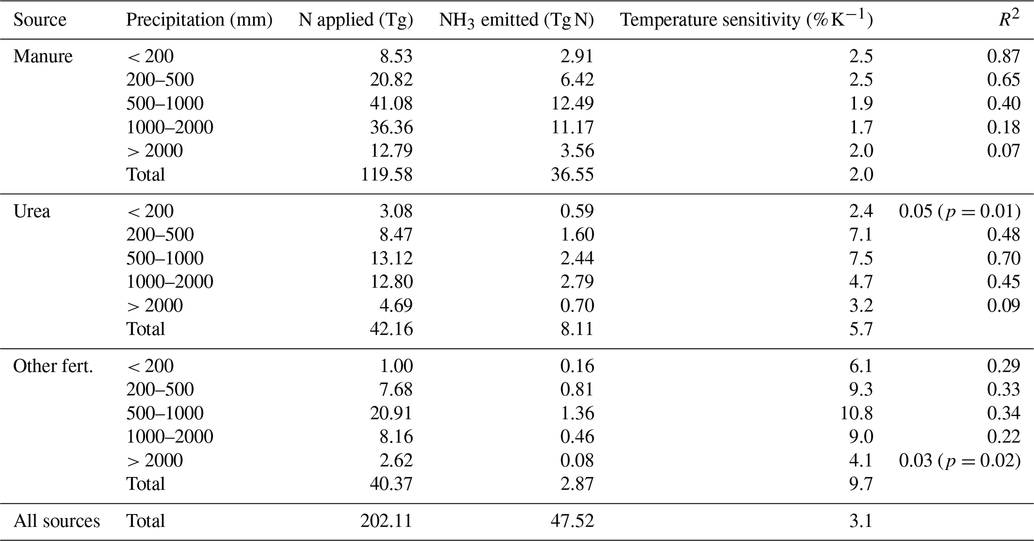
Although the linear temperature responses were significant (p≤0.02) for all categories, the R2 of the linear fits varied strongly between different sources and precipitation ranges. The R2 (0.07–0.87) values for manure were higher than for urea (0.05–0.70) or other fertilizers (0.03–0.34); the lowest R2 values below 0.1 were associated with regions with a yearly rainfall above 2000 mm or below 200 mm. The variation of R2 indicates that the annual temperature alone may be too coarse of a parameter for assessing the climate response of NH3 emissions.
Agricultural ammonia emissions are determined by both agricultural activity and environmental conditions. Both of these aspects of ammonia emissions have been incorporated into the process model FANv2, which embedded within the CESM simulates agricultural ammonia emissions globally. While we simulated the response of emissions from various agricultural processes to meteorological forcing on a yearly level, FANv2 could be used to estimate how the emissions respond to climate change on decadal to century timescales or how emissions respond to weather anomalies on hourly to daily timescales.
Global datasets have been used to quantify some regional agricultural practices in FANv2. For example, regional nitrogen excretion rates and synthetic fertilizer usage and type have been included. Regional agricultural practices also reflect variations in local meteorology, and these variations can be parameterized within an Earth system model. In FANv2 we use the local meteorological conditions to parameterize the timing of fertilizer application and the extent to which domestic animals excrete manure on pastures. The advantage of these meteorological-dependent parameterizations is that the impacts of climate change on these aspects of agricultural management are built implicitly into the model; the disadvantage is that these meteorological parameterizations do not always conform to regional agricultural practices.
Some regional aspects of agriculture remain simplified in the model. In particular, livestock manure is treated everywhere as a slurry and applied on land. This is likely to lead to uncertainties where handling manure as slurry is uncommon (e.g., Ndambi et al., 2019, for sub-Saharan Africa) or where a significant fraction of manure is discharged to waterways (e.g., Strokal et al., 2016, for China and IAEA, 2008, for Southeast Asia). Emissions from manure applications constitute only 10 %–15 % of the simulated total emissions outside Europe, North America, and China; nevertheless, with globally available information, FANv2 could be configured to include further details on regional agricultural practices and their changes.
Distinct from FANv2, most other available ammonia emission inventories make use of empirical factors relating ammonia emissions to livestock N excretion and fertilizer usage. The disadvantage of this approach is that it does not fully take into account variations in the environmental parameters that partially govern ammonia emissions. On the other hand, many emission inventories take regional and local agricultural practices into account. Over North America and Europe, the FANv2 NH3 emissions (3.5 and 4.8 Tg N yr−1, respectively) are within ∼ 25 % of established emission inventories (Table 2). This is perhaps not very surprising, as some of the simulated processes, such as handling manure as slurry, primarily reflect North American and European agricultural practices. Furthermore, some of the model parameters, such as average losses from animal housings and manure storage, were explicitly chosen to reproduce emission factors used in Europe. In contrast, for most other parts of the world, the FANv2 simulations differ from previous emission estimates.
In China, the FANv2 emissions (7.5 Tg N yr−1) are lower than the majority of recent global and regional estimates. The difference appears to be caused by the relatively low simulated emission losses from fertilizer in FANv2. Part of the difference can be attributed to differences in fertilizer use; 20.9 Tg N was applied in China in this study based on the CLM5 dataset (Sect. 2.5.2), which is less than the 22–25 Tg N in the inventories of Huang et al. (2012) and L. Zhang et al. (2018) and much less than the 37.1 Tg N in the inventory of X. Zhang et al. (2017). However, the lower fertilizer input alone is not enough to explain the lower NH3 emission in FANv2. Namely, FANv2 predicts that the fractions of urea or other fertilizers volatilized in China are similar to those in Europe or North America, in contrast to regional studies such as those by X. Zhang et al. (2017) and L. Zhang et al. (2018), which use higher emission factors compiled from empirical studies. The emission factor implied by FANv2 for China (Table 1) is 11 % for total fertilizer N and 14 % for urea. In comparison, the average emission factor for fertilizer N was 18.1 % in X. Zhang et al. (2017) and 16.6 % in L. Zhang et al. (2018).
It is difficult to isolate any particular factor that causes FANv2 to underestimate Chinese emission factors compared to the other inventories. Based on the sensitivity analysis (Sect. 3.3 and Sect. S5) in the Supplement, differences in soil adsorption, soil pH, and fertilizer incorporation could explain some of the discrepancy. Also, FANv2 and the CLM do not explicitly simulate rice paddies, which might play a role since rice cultivation is a major source of NH3 emissions in China (Xu et al., 2019), and the processes controlling NH3 volatilization in paddies are likely different from those in upland crops. For Chinese rice paddies, Wang et al. (2018) report an average emission factor of about 18 % for urea, which is higher than the factor calculated from FANv2 but not significantly higher than the overall emission factors used by X. Zhang et al. (2017) and L. Zhang et al. (2018). This suggests that the omission of rice paddies in FANv2 is not solely responsible for the discrepancy in emissions.
In contrast to China, in India FANv2 predicts higher NH3 emissions (7.5 Tg N yr−1) than previous inventories. In FANv2, the total volatilization loss of manure N is 35 % in India, which is ∼ 50 % higher than the 23 % emission factor used by Xu et al. (2018). The 27 % loss simulated for urea is also higher than the 19 % loss evaluated by Xu et al. (2018) but nevertheless similar to the 25 % emission factor used by Aneja et al. (2012). While the emissions from agricultural soils are similar in India in FANv2 and EDGAR, emissions from manure management in FANv2 are 7 times as high as those in EDGAR. A higher fraction of grazing in FANv2 would act to reduce the overall emissions, since the volatilization loss (Table 1) is 21 % for manure N excreted on pastures in FANv2, while the joint loss for barns, stores, and manure application is 57 % of the N excreted in barns. In FANv2 about 8 Tg of the total 13 Tg of manure N is excreted on pastures in India, which is limited by the maximum grazing fraction for mixed production systems in FANv2. Increasing the grazing fraction could reduce the simulated NH3 emissions by up to 1.8 Tg N, which would result in emissions similar to those in EDGAR.
It is unclear if a grazing fraction this high would be realistic, given that Mohini et al. (2016, cited by Prasad et al., 2017) report that in India the fraction of manure input on grazed fields is 35 %–45 % depending on the type of livestock. However, Prasad et al. (2017) note that a similar fraction of manure is used for fuel, and thus removed from the agricultural system. This is not taken into account in FANv2, but since the manure N in fuel is likely to be mainly in organic form with a low potential for ammonia volatilization, the reduction in NH3 emissions would likely be lower than the fraction of N in fuel.
The fractional volatilization losses (Table 1) were generally more variable regionally for synthetic fertilizers than for manure. The volatilization loss from synthetic fertilizers ranges between 6 % in Europe and 26 % in India. The different climates in Europe and India result in a variation of ∼ 15 %–27 % in the volatilization loss for urea. However, in Europe ∼ 20 % of fertilizer N was applied as urea and ∼ 30 % as nitrate according to the IFA fertilizer consumption data, while in India, the corresponding fractions were ∼ 85 % as urea and < 2 % as nitrate. Thus, the climate-driven difference in volatilization rates is amplified by the strong contrast in the usage of different fertilizers.
For manure, the overall fractional volatilization in FANv2 ranges from 23 % to 35 %. Manure emissions are split between emissions from grazing and emissions from manure housing, storage, and subsequent spreading. Large regional differences are apparent in the emissions from manure spreading, ranging from approximately 30 % of the TAN applied under cooler conditions (North America and Europe) to ∼ 75 % of the TAN applied in the warmest regions (Africa and India; Table 1). However, these regional variations in emissions are compensated for by regional variations in the extent of grazing, which ranges from ∼ 30 % in Europe (not shown) up to 75 % in Africa. The higher fraction of grazing in Africa compared to Europe is due to a longer grazing season, smaller proportion of non-grazing livestock (pigs, poultry), and larger proportion of pastoral livestock systems. Thus, in cooler regions animals spend more time in housing, so the overall emission factors due to housing, storage, and spreading are relatively high, while in warmer regions animals spend more time grazing and the emission factors are relatively low. The combination of regional practices and meteorological conditions acts to mute regional differences in manure NH3 emissions – contrary to the fertilizer NH3 emissions.
Globally, in FANv2, the simulated volatilization loss for fertilizers (13 %) is similar to the central estimate (14 %) given by Beusen et al. (2008). However, the average volatilization loss for manure (∼ 30 %) is about 60 % higher than the 19 % loss in the study of Beusen et al. (2008), wherein the manure emissions were based on the emission factors in Bouwman et al. (1997), hereafter B97. The difference stems largely from assumptions regarding geographical differences in NH3 volatilization from manure, which in B97 is represented by two aggregated regions.
In both FANv2 and B97 the overall volatilization loss from grazing animals is significantly less than the losses from barns and manure storage and spreading. For region I countries (developed countries), the 36 % volatilization loss from manure N excreted by cattle, pigs, and poultry in barns in B97 is similar to that in FANv2 (38 % in the same region, including losses in housing, storage, and spreading). The higher total volatilization loss (29 % in FANv2 vs. 21 % in B97) for manure N in region I countries is therefore explained by the higher volatilization rate for manure on pastures (15 % vs. 7 %) and the lower proportion of N excreted on pastures in Europe (28 % in FANv2 vs. 51 % for region I in B97). In North America, the fraction of N excreted on pastures is 50 % in FANv2, in agreement with B97.
In region II countries (developing countries), the fraction of N excreted on pastures in FANv2 (59 %) agrees with B97 (62 %). The corresponding volatilization rate is higher in FANv2 (18 %) than in B97 (13 %), but this difference alone is not enough to explain the difference in the total manure N volatilization. However, B97 assumed that the effect of higher average temperatures on animal housings in region II is compensated for by a lower TAN content in manure and therefore used the same emission factors for manure N excreted in barns for regions I and II. This resulted in a 21 % overall volatilization loss for both regions. In contrast, the TAN fraction in FANv2 is fixed at 60 % and therefore does not compensate for the higher volatilization rate (50 % for barns, storage, and spreading in region II). Together with the higher volatilization loss for grazing, this explains the higher volatilization loss (31 % vs. 21 %) in areas corresponding to region II in B97.
We have described a process-based model for evaluating ammonia volatilization losses from synthetic fertilizers and livestock wastes, evaluated the model with experimental data, and presented simulated global ammonia emissions obtained by coupling the process model into the land component of the Community Earth System Model (CESM). Compared to the initial version (Riddick et al., 2016), FANv2 improves the representation of soil processes as well as fertilization and manure management practices. The model evaluates ammonia emissions interactively with the simulated atmosphere and therefore responds to variations in the meteorological forcing. The impacts of different agricultural practices and their changes have also been incorporated into the model. Thus, FANv2, embedded within an Earth system model, represents a platform with which to investigate how ammonia emissions change as agricultural practices and climate change as we head into the future.
Comparison with data from 21 volatilization experiments shows that FANv2 successfully reproduces variations in volatilization between different types of manures and fertilizers. The model also reproduced variations stemming from environmental factors, albeit with a higher uncertainty. The mean model bias was small both within the categories and over the whole dataset.
Based on global simulations for 2010–2015, we estimate an average yearly NH3 emission of 48 Tg N consisting of 37 Tg from manure and 11 Tg from synthetic fertilizers. The volatilization losses correspond to 31 % of excreted manure N and 13 % applied fertilizer N. The simulated total emission is 30 %–40 % larger than previous estimates for 2010, which is mainly caused by higher simulated emissions from livestock wastes in Africa, India, and Latin America. The simulated emissions are in agreement with regional inventories for Europe and North America, and within the range of previous estimates for China.
In a preliminary estimate based on a statistical regression on geographical variations of simulated NH3 volatilization, the emission of NH3 was estimated to increase on average by ∼ 3 % for a 1 K increase in yearly mean temperature. This response includes the effect of increasing grazing and earlier crop planting dates in warmer climates.
Global NH3 emissions and their geographic distribution were sensitive to assumptions regarding livestock N excretion and the prevalence of grazing in mixed livestock production systems. Differences in these assumptions may explain some of the differences between FANv2 and earlier emission inventories.
The simulated emissions were coupled to the CAM-Chem chemistry–climate model, which allows for a further evaluation of the emission estimates via comparison with atmospheric observations. This path will be taken in a subsequent paper (Vira et al., 2020), which compares the atmospheric simulation with datasets of ammonia and ammonium concentrations and wet depositions.
| Variable | Equation | ||
| TAN | (A1) | ||
| Urea | (A2) | ||
| NA and NR | (A3) | ||
| Diagnostic concentrations | |||
| Quantity | Unit | Description | |
| [urea (aq, srf)] | g N m−3 | Dissolved urea at surface | (A4) |
| [TAN (aq, srf)] | g N m−3 | Dissolved TAN at surface | [TAN (aq, srf)]= |
| (A5) | |||
| where | |||
| χa=[NH3 (g,atm)] | |||
| x1=εKd | |||
| x2=Kdθ | |||
| Symbol | Unit | Description | Equation |
| Diffusion | |||
| ξgas | Tortuosity for gas-phase diffusion | (A6) | |
| (Millington and Quirk, 1961) | |||
| ξaq | Tortuosity for aqueous-phase diffusion | (A7) | |
| (Millington and Quirk, 1961) | |||
| m2 s−1 | Molecular diffusivity of in water | (A8) | |
| (Van Der Molen et al., 1990a) | |||
| m2 s−1 | Molecular diffusivity of NH3 in air | , (A9) | |
| where Mair=29.0, , Σairvi=20.1, | |||
| and p=1.0 | |||
| (Fuller et al., 1966) | |||
| Equilibrium constants | |||
| KH | NH3 (aq) ⇌ NH3 (g) | (A10) | |
| (Sutton et al., 1994), where Tref=298.15 K | |||
| mol L−1 | (A11) | ||
| (Sutton et al., 1994), where Tref is as in Eq. (A10) | |||
| [NH3 (g)]∕[TAN (aq)] | (A12) | ||
| Kd | [TAN (s)]∕[TAN (aq)] | Kd=1.0(A13) | |
| Symbol | Unit | Description | Equation |
| Decomposition rates | |||
| s−1 | Nitrification rate | ,(A14) | |
| where (Riddick et al., 2016) | |||
| and the gravimetric soil moisture | |||
| Σ(Tg) | Temperature response function | , (A15) | |
| where topt=301 K and , and aΣ=2.4 | |||
| (Stange and Neue, 2009) | |||
| Π(θ) | Moisture response function | ,(A16) | |
| where mcrit=0.12(Stange and Neue, 2009) | |||
| and θg is as in Eq. (A14) | |||
| ka, kr | s−1 | Decomposition rate for NA and NR | ka,r=Ba,rTR(Tg)Pψ(ψ),(A17) |
| where and | |||
| (Gilmour et al., 2003; Vigil and Kissel, 1995) | |||
| TR | Temperature dependence of ka and kb | ,(A18) | |
| where tr1=0.0106 and | |||
| (Vigil and Kissel, 1995) | |||
| Pψ | Soil moisture dependency ka and kb | ,(A19) | |
| where ψ is the soil matric potential (MPa), | |||
| and | |||
| (Lawrence et al., 2018) | |||
| ku | s−1 | Decomposition rate for NU | (A20) |
| Agehara and Warncke (2005) | |||
| Symbol | Unit | Description | Equation |
| Approximate expressions for the volatilization rate | |||
| Fdry | NH3 flux in nearly dry soil | (A21) | |
| for | |||
| Fsat | NH3 flux in nearly saturated soil | (A22) | |
| for and θ∼θs | |||
Table B1Experimental studies used in model evaluation (Sect. 2.6). Soil pH and cation exchange capacity are shown when reported. The synthetic fertilizers are abbreviated as AS (ammonium sulfate), CAN (calcium ammonium nitrate), and DAP (diammonium phosphate). The measurements of Bittman et al. (2005) and Dowling et al. (2008) were extracted from the ALFAM2 database (Hafner et al., 2018).
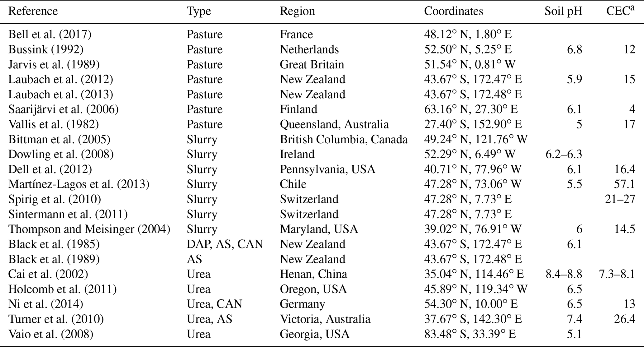
a Cation exchange capacity (cmolc kg−1).
Table B2Main datasets used in this study. In addition, the simulations use the standard input datasets of CAM4 (Lamarque et al., 2012) and CLM5 (Lawrence et al., 2018).
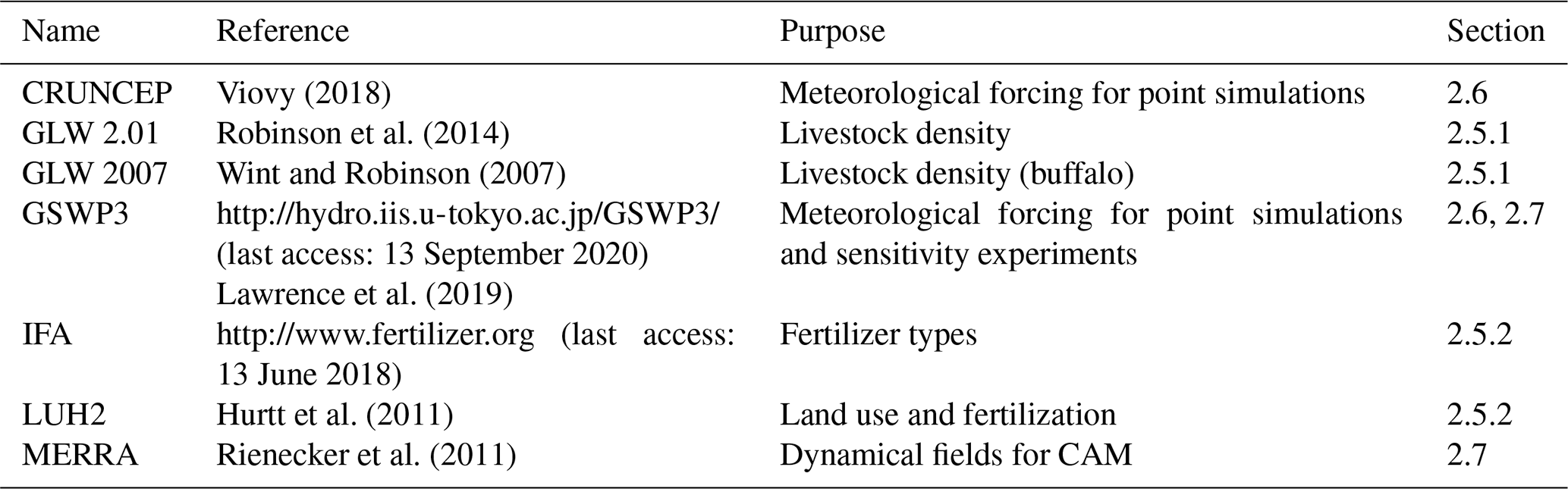
The Community Earth System Model, including the Community Land Model (CLM), is available at http://www.cesm.ucar.edu (last access: 13 September 2020). The modified version of CLM used in this paper is available at https://doi.org/10.5281/zenodo.3841776 (Vira et al., 2019). The full modified version of CESM, including changes to CAM and the coupler interface, requires access to the CAM development repository, which can be granted by UCAR upon agreement with the terms of use. Potential users are suggested to contact the authors for the latest version of the code. The simulated monthly NH3 emissions and model input data prepared for this study are available at https://doi.org/10.5281/zenodo.3841723 (Vira et al., 2020) and included in the Supplement; other model outputs are available on request.
The supplement related to this article is available online at: https://doi.org/10.5194/gmd-13-4459-2020-supplement.
JV, PH, and JM formulated the model. JV and WRW implemented the model in CLM. JV designed and performed the simulation experiments and analyzed the output with contributions from PH. JV and PH prepared the paper with contributions from JM and WRW.
The authors declare that they have no conflict of interest.
This work was funded in part by the Department of Energy (no. DE-SC0016361) and was supported in part by the National Center for Atmospheric Research, which is a major facility sponsored by the National Science Foundation, under cooperative agreement no. 1852977. Computing resources (https://doi.org/10.5065/D6RX99HX) were provided by the Climate Simulation Laboratory at NCAR's Computational and Information Systems Laboratory, sponsored by the National Science Foundation and other agencies. William R. Wieder was supported by the US Department of Agriculture NIFA award number 2015-67003-23485 and the Environmental Protection Agency's National Center for Environmental Assessment through an interagency agreement with the National Science Foundation and the National Center for Atmospheric Research (no. DW-49-92447301-0). The authors thank Susan Cheng, Susan Riha, and Jinyun Tang for valuable discussions and Marje Prank for comments on the paper. We also thank Rongting Xu and the two anonymous reviewers for their feedback on the paper.
This research has been supported by the U.S. Department of Energy (grant no. DE-SC0016361), the National Science Foundation (grant no. 1852977), the U.S. Department of Agriculture (grant no. 2015-67003-23485), and the U.S. Environmental Protection Agency (grant no. DW-49-92447301-0).
This paper was edited by Jason Williams and reviewed by Rongting Xu and two anonymous referees.
Agehara, S. and Warncke, D. D.: Soil Moisture and Temperature Effects on Nitrogen Release from Organic Nitrogen Sources, Soil Sci. Soc. Am. J., 69, 1844–1855, https://doi.org/10.2136/sssaj2004.0361, 2005. a, b, c
Aneja, V. P., Schlesinger, W. H., Erisman, J. W., Behera, S. N., Sharma, M., and Battye, W.: Reactive nitrogen emissions from crop and livestock farming in India, Atmos. Environ., 47, 92–103, https://doi.org/10.1016/j.atmosenv.2011.11.026, 2012. a, b
Badger, A. M. and Dirmeyer, P. A.: Climate response to Amazon forest replacement by heterogeneous crop cover, Hydrol. Earth Syst. Sci., 19, 4547–4557, https://doi.org/10.5194/hess-19-4547-2015, 2015. a
Bash, J. O., Cooter, E. J., Dennis, R. L., Walker, J. T., and Pleim, J. E.: Evaluation of a regional air-quality model with bidirectional NH3 exchange coupled to an agroecosystem model, Biogeosciences, 10, 1635–1645, https://doi.org/10.5194/bg-10-1635-2013, 2013. a
Battye, W., Aneja, V. P., and Schlesinger, W. H.: Is nitrogen the next carbon?, Earths Future, 5, 894–904, https://doi.org/10.1002/2017EF000592, 2017. a
Bear, J. and Verruijt, A.: Modeling groundwater flow and pollution, D. Reidel Publishing Company, Dordrecht, 1987. a
Bell, M., Flechard, C., Fauvel, Y., Häni, C., Sintermann, J., Jocher, M., Menzi, H., Hensen, A., and Neftel, A.: Ammonia emissions from a grazed field estimated by miniDOAS measurements and inverse dispersion modelling, Atmos. Meas. Tech., 10, 1875–1892, https://doi.org/10.5194/amt-10-1875-2017, 2017. a, b
Beusen, A. H., Bouwman, A. F., Heuberger, P. S., Van Drecht, G., and Van Der Hoek, K. W.: Bottom-up uncertainty estimates of global ammonia emissions from global agricultural production systems, Atmos. Environ., 42, 6067–6077, https://doi.org/10.1016/j.atmosenv.2008.03.044, 2008. a, b, c, d, e, f, g, h
Bittman, S., Van Vliet, L. J., Kowalenko, C. G., McGinn, S., Hunt, D. E., and Bounaix, F.: Surface-banding liquid manure over aeration slots: A new low-disturbance method for reducing ammonia emissions and improving yield of perennial grasses, Agron. J., 97, 1304–1313, https://doi.org/10.2134/agronj2004.0277, 2005. a, b
Black, A. S., Sherlock, R. R., Smith, N. P., Cameron, K. C., and Goh, K. M.: Effects of form of nitrogen, season, and urea application rate on ammonia volatilisation from pastures, New Zeal. J. Agr. Res., 28, 469–474, https://doi.org/10.1080/00288233.1985.10417992, 1985. a, b, c, d
Black, A. S., Sherlock, R. R., Smith, N. P., and Cameron, K. C.: Ammonia volatilisation from urea broadcast in spring on to autumn-sown wheat, New Zeal. J. Crop Hort., 17, 175–182, https://doi.org/10.1080/01140671.1989.10428028, 1989. a, b
Bouwman, A. F., Lee, D. S., Asman, W. A., Dentener, F. J., Van Der Hoek, K. W., and Olivier, J. G.: A global high-resolution emission inventory for ammonia, Global Biogeochem. Cy., 11, 561–587, https://doi.org/10.1029/97GB02266, 1997. a, b
Bouwman, A. F., Boumans, L. J. M., and Batjes, N. H.: Estimation of global NH3 volatilization loss from synthetic fertilizers and animal manure applied to arable lands and grasslands, Global Biogeochem. Cy., 16, 8-1–8-14, https://doi.org/10.1029/2000GB001389, 2002. a, b, c, d, e, f
Bouwman, A. F., Van Der Hoek, K. W., Eickhout, B., and Soenario, I.: Exploring changes in world ruminant production systems, Agr. Syst., 84, 121–153, https://doi.org/10.1016/j.agsy.2004.05.006, 2005. a
Buss, S. R., Herbert, A. W., Morgan, P., Thornton, S. F., and Smith, J. W. N.: A review of ammonium attenuation in soil and groundwater, Q. J. Eng. Geol. Hydroge., 37, 347–359, 2004. a, b
Bussink, D. W.: Ammonia volatilization from grassland receiving nitrogen fertilizer and rotationally grazed by dairy cattle, Fert. Res., 33, 257–265, https://doi.org/10.1007/bf01050881, 1992. a, b, c, d, e
Bussink, D. W., Huijsmans, J. F. M., and Ketelaars, J. J. M. H.: Ammonia volatilization from nitric-acid-treated cattle slurry surface applied to grassland, Netherlands Journal of Agricultural Science, 42, https://doi.org/10.18174/njas.v42i4.590, 1994. a
Cai, G. X., Chen, D. L., Ding, H., Pacholski, A., Fan, X. H., and Zhu, Z. L.: Nitrogen losses from fertilizers applied to maize, wheat and rice in the North China Plain, Nutr. Cycl. Agroecosys., 63, 187–195, https://doi.org/10.1023/A:1021198724250, 2002. a
Castesana, P. S., Dawidowski, L. E., Finster, L., Gómez, D. R., and Taboada, M. A.: Ammonia emissions from the agriculture sector in Argentina; 2000–2012, Atmos. Environ., 178, 293–304, https://doi.org/10.1016/j.atmosenv.2018.02.003, 2018. a, b, c, d
Cooter, E. J., Bash, J. O., Walker, J. T., Jones, M. R., and Robarge, W.: Estimation of NH3 bi-directional flux from managed agricultural soils, Atmos. Environ., 44, 2107–2115, https://doi.org/10.1016/j.atmosenv.2010.02.044, 2010. a
Crippa, M., Guizzardi, D., Muntean, M., Schaaf, E., Dentener, F., van Aardenne, J. A., Monni, S., Doering, U., Olivier, J. G. J., Pagliari, V., and Janssens-Maenhout, G.: Gridded emissions of air pollutants for the period 1970–2012 within EDGAR v4.3.2, Earth Syst. Sci. Data, 10, 1987–2013, https://doi.org/10.5194/essd-10-1987-2018, 2018. a, b
Dell, C. J., Kleinman, P. J., Schmidt, J. P., and Beegle, D. B.: Low-Disturbance Manure Incorporation Effects on Ammonia and Nitrate Loss, J. Environ. Qual., 41, 928–937, https://doi.org/10.2134/jeq2011.0327, 2012. a, b
Delon, C., Galy-Lacaux, C., Boone, A., Liousse, C., Serça, D., Adon, M., Diop, B., Akpo, A., Lavenu, F., Mougin, E., and Timouk, F.: Atmospheric nitrogen budget in Sahelian dry savannas, Atmos. Chem. Phys., 10, 2691–2708, https://doi.org/10.5194/acp-10-2691-2010, 2010. a
Dentener, F., Drevet, J., Lamarque, J. F., Bey, I., Eickhout, B., Fiore, A. M., Hauglustaine, D., Horowitz, L. W., Krol, M., Kulshrestha, U. C., Lawrence, M., Galy-Lacaux, C., Rast, S., Shindell, D., Stevenson, D., Van Noije, T., Atherton, C., Bell, N., Bergman, D., Butler, T., Cofala, J., Collins, B., Doherty, R., Ellingsen, K., Galloway, J., Gauss, M., Montanaro, V., Müller, J. F., Pitari, G., Rodriguez, J., Sanderson, M., Solmon, F., Strahan, S., Schultz, M., Sudo, K., Szopa, S., and Wild, O.: Nitrogen and sulfur deposition on regional and global scales: A multimodel evaluation, Global Biogeochem. Cy., 20, GB4003, https://doi.org/10.1029/2005GB002672, 2006. a
Dowling, C., Curran, T., and Lanigan, G.: The effect of application timing on ammonia emissions from cattle slurry in Ireland, in: 13th Int. RAMIRAN Proceedings, Albena, 11–14 June 2008, p. 4, 2008. a, b
Duprè, C., Stevens, C. J., Ranke, T., Bleekers, A., Peppler-Lisbach, C., Gowing, D. J. G., Dise, N. B., E, D., Bobbink, R., and Diekmann, M.: Changes in species richness and composition in European acidic grasslands over the past 70 years: the contribution of cumulative atmospheric nitrogen deposition, Glob. Change Biol., 16, 344–357, https://doi.org/10.1111/j.1365-2486.2009.01982.x, 2010. a
EEA: EMEP/EEA air pollutant emission inventory guidebook 2016, Tech. rep., European Environmental Agency, Publications Office of the European Union, Luxembourg, 2016. a
FAO/IIASA/ISCRIC/IIS-CAS/JRC: Harmonized World Soil Database (version 1.1), FAO, Rome, Italy and IIASA, Laxenburg, Austria, 2009.
Fuller, E. N., Schettler, P. D., and Giddings, J. C.: A new method for prediction of binary gas-phase diffusion coefficients, Ind. Eng. Chem., 58, 18–27, https://doi.org/10.1021/ie50677a007, 1966. a
Genermont, S. and Cellier, P.: A mechanistic model for estimating amnmonia volatilization from slurry applied to bare soil, Agr. Forest Meteorol., 88, 145–167, 1997. a
Gilmour, J. T., Cogger, C. G., Jacobs, L. W., Evanylo, G. K., and Sullivan, D. M.: Decomposition and plant-available nitrogen in biosolids, J. Environ. Qual., 32, 1498–1507, 2003. a
Giltrap, D., Saggar, S., Rodriguez, J., and Bishop, P.: Modelling NH3 volatilisation within a urine patch using NZ-DNDC, Nutr. Cycl. Agroecosys., 108, 267–277, https://doi.org/10.1007/s10705-017-9854-x, 2017. a
Gyldenkærne, S., Skjøth, C. A., Hertel, O., and Ellermann, T.: A dynamical ammonia emission parameterization for use in air pollution models, J. Geophys. Res.-Atmos., 110, 1–14, https://doi.org/10.1029/2004JD005459, 2005. a, b, c, d
Hafner, S. D., Pacholski, A., Bittman, S., Burchill, W., Bussink, W., Chantigny, M., Carozzi, M., Génermont, S., Häni, C., Hansen, M. N., Huijsmans, J., Hunt, D., Kupper, T., Lanigan, G., Loubet, B., Misselbrook, T., Meisinger, J. J., Neftel, A., Nyord, T., Pedersen, S. V., Sintermann, J., Thompson, R. B., Vermeulen, B., Vestergaard, A. V., Voylokov, P., Williams, J. R., and Sommer, S. G.: The ALFAM2 database on ammonia emission from field-applied manure: Description and illustrative analysis, Agr. Forest Meteorol., 258, 66–79, https://doi.org/10.1016/j.agrformet.2017.11.027, 2018. a
Hamaoui-Laguel, L., Meleux, F., Beekmann, M., Bessagnet, B., Génermont, S., and Celier, P.: Modelling agricultural ammonia emissions : impact on particulate matter formation, Conference “Nitrogen & global change: key findings and future challenges”, pp. 3–4, 11–15 April 2011, Edingbourgh, UK, 2011. a
Harper, L. A.: Ammonia: Measurement Issues, in: Micrometeorology in Agricultural Systems, Agronomy Monograph no. 47, edited by: Hatfield, J. L. and Baker, J. M., American Society of Agronomy, Inc., Crop Science Society of America, Inc, and Soil Science Society of America, Inc. Madison, Wisconsin, USA, pp. 345–379, https://doi.org/10.2134/agronmonogr47.c15, 2005. a
Heald, C. L., Collett Jr., J. L., Lee, T., Benedict, K. B., Schwandner, F. M., Li, Y., Clarisse, L., Hurtmans, D. R., Van Damme, M., Clerbaux, C., Coheur, P.-F., Philip, S., Martin, R. V., and Pye, H. O. T.: Atmospheric ammonia and particulate inorganic nitrogen over the United States, Atmos. Chem. Phys., 12, 10295–10312, https://doi.org/10.5194/acp-12-10295-2012, 2012. a
Holcomb, J. C., Sullivan, D. M., Horneck, D. A., and Clough, G. H.: Effect of Irrigation Rate on Ammonia Volatilization, Soil Sci. Soc. Am. J., 75, 2341–2347, https://doi.org/10.2136/sssaj2010.0446, 2011. a, b, c
Huang, X., Song, Y., Li, M., Li, J., Huo, Q., Cai, X., Zhu, T., Hu, M., and Zhang, H.: A high-resolution ammonia emission inventory in China, Global Biogeochem. Cy., 26, 1–14, https://doi.org/10.1029/2011GB004161, 2012. a
Hurtt, G. C., Chini, L. P., Frolking, S., Betts, R. A., Feddema, J., Fischer, G., Fisk, J. P., Hibbard, K., Houghton, R. A., Janetos, A., Jones, C. D., Kindermann, G., Kinoshita, T., Klein Goldewijk, K., Riahi, K., Shevliakova, E., Smith, S., Stehfest, E., Thomson, A., Thornton, P., van Vuuren, D. P., and Wang, Y. P.: Harmonization of land-use scenarios for the period 1500–2100: 600 years of global gridded annual land-use transitions, wood harvest, and resulting secondary lands, Climatic Change, 109, 117–161, https://doi.org/10.1007/s10584-011-0153-2, 2011. a, b
IAEA: Guidelines for sustainable manure management in Asian livestock production systems, Tech. Rep. IAEA-TECDOC-1582, IAEA, Vienna, 2008. a
IPCC: 2006 IPCC Guidelines for National Greenhouse Gas Inventories, IGES, Hayama, Kanagawa, Japan, Japan, 2006. a
Jarvis, S. C., Sherwood, M., and Steenvoorden, J.: Nitrogen losses from animal manures: from grazed pastures and from applied slurry, in: Animal Manure on Grassland and Fodder Crops. Fertilizer or Waste?, edited by: Van Der Meer, H. G., Unwin, R. J., Van Dijk, T. A., and Ennik, G. C., Martinus Nijhoff Publishers, Dordrecht, pp. 195–212, 1987. a
Jarvis, S. C., Hatch, D. J., and Roberts, D. H.: The effects of grassland mangement on nitrogen losses from grazedswards through ammonia volatilization: the relationship to excretal N returns from cattle, J. Agr. Sci., 112, 205–216, 1989. a, b
Kang, Y., Liu, M., Song, Y., Huang, X., Yao, H., Cai, X., Zhang, H., Kang, L., Liu, X., Yan, X., He, H., Zhang, Q., Shao, M., and Zhu, T.: High-resolution ammonia emissions inventories in China from 1980 to 2012, Atmos. Chem. Phys., 16, 2043–2058, https://doi.org/10.5194/acp-16-2043-2016, 2016. a
Klimont, Z. and Brink, C.: Modeling of emissions of air pollutants and greenhouse gases from agricultural sources in Europe, Tech. rep., International Institute for Applied Systems Analysis, Laxenburg, Austria, 2004. a
Kurokawa, J., Ohara, T., Morikawa, T., Hanayama, S., Janssens-Maenhout, G., Fukui, T., Kawashima, K., and Akimoto, H.: Emissions of air pollutants and greenhouse gases over Asian regions during 2000–2008: Regional Emission inventory in ASia (REAS) version 2, Atmos. Chem. Phys., 13, 11019–11058, https://doi.org/10.5194/acp-13-11019-2013, 2013. a, b
Lamarque, J.-F., Emmons, L. K., Hess, P. G., Kinnison, D. E., Tilmes, S., Vitt, F., Heald, C. L., Holland, E. A., Lauritzen, P. H., Neu, J., Orlando, J. J., Rasch, P. J., and Tyndall, G. K.: CAM-chem: description and evaluation of interactive atmospheric chemistry in the Community Earth System Model, Geosci. Model Dev., 5, 369–411, https://doi.org/10.5194/gmd-5-369-2012, 2012. a, b
Laubach, J., Taghizadeh-Toosi, A., Sherlock, R. R., and Kelliher, F. M.: Measuring and modelling ammonia emissions from a regular pattern of cattle urine patches, Agr. Forest Meteorol., 156, 1–17, https://doi.org/10.1016/j.agrformet.2011.12.007, 2012. a, b, c
Laubach, J., Taghizadeh-Toosi, A., Gibbs, S. J., Sherlock, R. R., Kelliher, F. M., and Grover, S. P. P.: Ammonia emissions from cattle urine and dung excreted on pasture, Biogeosciences, 10, 327–338, https://doi.org/10.5194/bg-10-327-2013, 2013. a, b
Lawrence, D., Fisher, R., Koven, C., Oleson, K., Swenson, S., and Vertenstein, M.: Technical Description of version 5.0 of the Community Land Model (CLM), Tech. rep., National Center for Atmospheric Research, Boulder, CO, 2018. a, b, c, d
Lawrence, D. M., Hurtt, G. C., Arneth, A., Brovkin, V., Calvin, K. V., Jones, A. D., Jones, C. D., Lawrence, P. J., de Noblet-Ducoudré, N., Pongratz, J., Seneviratne, S. I., and Shevliakova, E.: The Land Use Model Intercomparison Project (LUMIP) contribution to CMIP6: rationale and experimental design, Geosci. Model Dev., 9, 2973–2998, https://doi.org/10.5194/gmd-9-2973-2016, 2016. a
Lawrence, D. M., Fisher, R. M., Koven, C. D., Oleson, K. W., Swenson, S. C., Bonan, G., Ghimere, B., van Kampenhout, L., Kennedy, D., Kluzek, E., Lawrence, P. J., Li, F., Li, H., Lombardozzi, D. L., Riley, W. J., Sacks, W. J., Shi, M., Vertenstein, M., Wieder, W. R., Xu, C., Ali, A. A., Badger, A. M., Bisht, G., van den Broeke, M., Brunke, M. A., Burns, S. P., Buzan, J., Clark, M., Craig, A., Dahlin, K., Drewniak, B., Fisher, J. B., Flanner, M., Fox, A. M., Gentine, P. G., Hoffman, F., Keppel-Aleks, G., Knox, R., Kumar, S., Lenaerts, J., Leung, L. R., Lipscomb, W. H., Lu, Y., Pandey, A., Pelletier, J. D., Perket, J., Randerson, J. T., Ricciuto, D. M., Sanderson, B. M., Slater, A., Subin, Z. M., Tang, J., Thomas, R. Q., Val Martin, M., and Zeng, X.: Community Land Model version 5: Description of new features, benchmarking, and impact of forcing uncertainty, J. Adv. Model. Earth Syst., 11, 4245–4287, https://doi.org/10.1029/2018MS001583, 2019. a, b, c, d, e
Levis, S., Bonan, G. B., Kluzek, E., Thornton, P. E., Jones, A., Sacks, W. J., and Kucharik, C. J.: Interactive crop management in the Community Earth System Model (CESM1): Seasonal influences on land–atmosphere fluxes, J. Climate, 25, 4839–4859, 2012. a
Levis, S., Badger, A., Drewniak, B., Nevison, C., and Ren, X.: CLMcrop yields and water requirements: avoided impacts by choosing RCP 4.5 over 8.5, Climatic Change, 146, 501–515, 2018. a, b
Li, C., Salas, W., Zhang, R., Krauter, C., Rotz, A., and Mitloehner, F.: Manure-DNDC: A biogeochemical process model for quantifying greenhouse gas and ammonia emissions from livestock manure systems, Nutr. Cycl. Agroecosys., 93, 163–200, https://doi.org/10.1007/s10705-012-9507-z, 2012. a
Li, J., Yang, H., Zhou, F., Zhang, X., Luo, J., Li, Y., Lindsey, S., Shi, Y., He, H., and Zhang, X.: Effects of maize residue return rate on nitrogen transformations and gaseous losses in an arable soil, Agr. Water Manage., 211, 132–141, https://doi.org/10.1016/j.agwat.2018.09.049, 2019. a
Lombardozzi, D. L., Lu, Y., Lawrence, P. J., Lawrence, D. M., Swenson, S., Oleson, K. W., Wieder, W. R., and Ainsworth, E. A.: Simulating Agriculture in the Community Land Model Version 5, J. Geophys. Res.-Biogeo., 125, 1–19, https://doi.org/10.1029/2019jg005529, 2020. a, b
Lorimor, J., Powers, W., and Sutton, A.: Manure Characteristics, in: Manure Management Systems Series, Midwest Plan Service, Ames, Iowa, pp. 1–23, 2001. a
Manzoni, S. and Porporato, A.: Soil carbon and nitrogen mineralization: Theory and models across scales, Soil Biol. Biochem., 41, 1355–1379, https://doi.org/10.1016/j.soilbio.2009.02.031, 2009. a
Martínez-Lagos, J., Salazar, F., Alfaro, M., and Misselbrook, T.: Ammonia volatilization following dairy slurry application to a permanent grassland on a volcanic soil, Atmos. Environ., 80, 226–231, https://doi.org/10.1016/j.atmosenv.2013.08.005, 2013. a
Meisinger, J. J. and Jokela, W. E.: Ammonia volatilization from dairy and poultry manure, in: Proceedings from managing nutrients and pathogens from animal agriculture, Camp Hill, Pennsylvania, 28–30 March 2000, pp. 334–354, 2000. a
Millington, R. J. and Quirk, J. P.: Permeability of porous solids, T. Faraday Soc., 57, 1200–1207, 1961. a, b, c
Misselbrook, T., Misselbrook, T., Scholefield, D., and Parkinson, R.: Using time domain reflectometry to characterize cattle and pig slurry infiltration into soil, Soil Use and Manage., 21, 167–172, https://doi.org/10.1111/j.1475-2743.2005.tb00121.x, 2005a. a
Misselbrook, T. H., Nicholson, F. A., and Chambers, B. J.: Predicting ammonia losses following the application of livestock manure to land, Bioresource Technol., 96, 159–168, https://doi.org/10.1016/j.biortech.2004.05.004, 2005b. a, b, c
Mohini, M., Mondal, G., Thakur, S. S., and Gupta, S.: Trends in methane emission from Indian livestock, in: Proceedings of XVI Biennial Animal Nutrition Conference on Innovative Approaches for Animal Feeding and Nutritional Research, NDRI, 6–8 February 2016, Karnal, 2016. a
Móring, A., Vieno, M., Doherty, R. M., Laubach, J., Taghizadeh-Toosi, A., and Sutton, M. A.: A process-based model for ammonia emission from urine patches, GAG (Generation of Ammonia from Grazing): description and sensitivity analysis, Biogeosciences, 13, 1837–1861, https://doi.org/10.5194/bg-13-1837-2016, 2016. a, b
Muñoz, E., Navia, R., Zaror, C., and Alfaro, M.: Ammonia emissions from livestock production in Chile: an inventory and uncertainty analysis, J. Soil Sci. Plant Nut., 16, 60–75, https://doi.org/10.4067/S0718-95162016005000005, 2016. a, b
Ndambi, O. A., Pelster, D. E., Owino, J. O., de Buisonjé, F., and Vellinga, T.: Manure Management Practices and Policies in Sub-Saharan Africa: Implications on Manure Quality as a Fertilizer, Frontiers in Sustainable Food Systems, 3, 29, https://doi.org/10.3389/fsufs.2019.00029, 2019. a
Ni, K., Pacholski, A., and Kage, H.: Ammonia volatilization after application of urea to winter wheat over 3 years affected by novel urease and nitrification inhibitors, Agr. Ecosyst. Environ., 197, 184–194, https://doi.org/10.1016/j.agee.2014.08.007, 2014. a
Pain, B. F., Phillips, V. R., Clarkson, C. R., and Klarenbeek, J. V.: Loss of nitrogen through ammonia volatilisation during and following the application of pig or cattle slurry to grassland, J. Sci. Food Agr., 47, 1–12, https://doi.org/10.1002/jsfa.2740470102, 1989. a
Pan, B., Lam, S. K., Mosier, A., Luo, Y., and Chen, D.: Ammonia volatilization from synthetic fertilizers and its mitigation strategies: A global synthesis, Agr. Ecosyst. Environ., 232, 283–289, https://doi.org/10.1016/j.agee.2016.08.019, 2016. a
Pang, P. C., Hedlin, R. A., and Cho, C. M.: Transformation and movement of band-applied urea, ammonium sulfate, and ammonium hydroxide during incubation in several manitoba soils, Can. J. Soil Sci., 53, 331–341, 1973. a
Paulot, F., Jacob, D. J., Pinder, R. W., Bash, J. O., Travis, K., and Henze, D. K.: Ammonia emissions in the United States, european union, and China derived by high-resolution inversion of ammonium wet deposition data: Interpretation with a new agricultural emissions inventory (MASAGE_NH3), J. Geophys. Res., 119, 4343–4364, https://doi.org/10.1002/2013JD021130, 2014. a, b
Paulot, F., Ginoux, P., Cooke, W. F., Donner, L. J., Fan, S., Lin, M.-Y., Mao, J., Naik, V., and Horowitz, L. W.: Sensitivity of nitrate aerosols to ammonia emissions and to nitrate chemistry: implications for present and future nitrate optical depth, Atmos. Chem. Phys., 16, 1459–1477, https://doi.org/10.5194/acp-16-1459-2016, 2016. a
Payne, R. J., Dise, N. B., Field, C. D., Dore, A. J., Caporn, S. J., and Stevens, C. J.: Nitrogen deposition and plant biodiversity: past, present, and future, Front. Ecol. Environ., 15, 431–436, https://doi.org/10.1002/fee.1528, 2017. a
Petersen, S. O. and Andersen, M. N.: Influence of soil water potential and slurry type on denitrification activity, Soil Biol. Biochem., 28, 977–980, https://doi.org/10.1016/0038-0717(96)00067-3, 1996. a
Pinder, R. W., Pekney, N. J., Davidson, C. I., and Adams, P. J.: A process-based model of ammonia emissions from dairy cows: Improved temporal and spatial resolution, Atmos. Environ., 38, 1357–1365, https://doi.org/10.1016/j.atmosenv.2003.11.024, 2004. a
Pleim, J. E., Ran, L., Appel, W., Shephard, M. W., and Cady-Pereira, K.: New Bidirectional Ammonia Flux Model in an Air Quality Model Coupled With an Agricultural Model, J. Adv. Model. Earth Sy., 11, 2934–2957, https://doi.org/10.1029/2019ms001728, 2019. a
Potter, P., Ramankutty, N., Bennett, E. M., and Donner, S. D.: Characterizing the spatial patterns of global fertilizer application and manure production, Earth Interact., 14, 1–22, https://doi.org/10.1175/2009EI288.1, 2010. a
Prasad, C. S., Gowda, N. K. S., Anandan, S., Sharma, K., and Mohini, M.: Reactive Nitrogen in Environment vis-à-vis Livestock Production System: Possible Remedies, in: The Indian Nitrogen Assessment, edited by: Abrol, Y. P., Adhya, T. K., Aneja, V. P., Raghuram, N., Pathak, H., Kulshrestha, U., Sharma, C., and Singh, B., Elsevier, 235–247, https://doi.org/10.1016/B978-0-12-811836-8.00016-1, 2017. a, b
Rachhpal-Singh and Nye, P.: A model of ammonia volatilization from applied urea. I. development of the model, J. Soil Sci., 37, 9–20, https://doi.org/10.1111/j.1365-2389.1986.tb00002.x, 1986. a
Riddick, S., Ward, D., Hess, P., Mahowald, N., Massad, R., and Holland, E.: Estimate of changes in agricultural terrestrial nitrogen pathways and ammonia emissions from 1850 to present in the Community Earth System Model, Biogeosciences, 13, 3397–3426, https://doi.org/10.5194/bg-13-3397-2016, 2016. a, b, c, d, e, f, g
Rienecker, M. M., Suarez, M. J., Gelaro, R., Todling, R., Bacmeister, J., Liu, E., Bosilovich, M. G., Schubert, S. D., Takacs, L., Kim, G.-K., Bloom, S., Chen, J., Collins, D., Conaty, A., da Silva, A., Gu, W., Joiner, J., Koster, R. D., Lucchesi, R., Molod, A., Owens, T., Pawson, S., Pegion, P., Redder, C. R., Reichle, R., Robertson, F. R., Ruddick, A. G., Sienkiewicz, M., and Woollen, J.: MERRA: NASA's modern-era retrospective analysis for research and applications, J. Climate, 24, 3624–3648, 2011. a
Robinson, T. P., Thornton, P. K., Franceschini, G., Kruska, R. L., Chiozza, F., Notenbaert, A., Cecchi, G., Herrero, M., Epprecht, M., Fritz, S., You, L., Conchedda, G., and See, L.: Global livestock production systems, FAO and ILRI, Rome, 2011. a
Robinson, T. P., Wint, G. R. W., Conchedda, G., Van Boeckel, T. P., Ercoli, V., Palamara, E., Cinardi, G., D'Aietti, L., Hay, S. I., and Gilbert, M.: Mapping the global distribution of livestock, PloS ONE, 9, e96084, https://doi.org/10.1371/journal.pone.0096084, 2014. a, b
Rochette, P., Angers, D. A., Chantigny, M. H., Gasser, M.-O., MacDonald, J. D., Pelster, D. E., and Bertrand, N.: Ammonia Volatilization and Nitrogen Retention: How Deep to Incorporate Urea?, J. Environ. Qual., 42, 1635, https://doi.org/10.2134/jeq2013.05.0192, 2013. a, b
Ryden, J., Whitehead, D., Lockyer, D., Thompson, R., Skinner, J., and Garwood, E.: Ammonia emission from grassland and livestock production systems in the UK, Environ. Pollut., 48, 173–184, https://doi.org/10.1016/0269-7491(87)90032-7, 1987. a
Saarijärvi, K., Mattila, P. K., and Virkajärvi, P.: Ammonia volatilization from artificial dung and urine patches measured by the equilibrium concentration technique (JTI method), Atmos. Environ., 40, 5137–5145, https://doi.org/10.1016/j.atmosenv.2006.03.052, 2006. a
Sadeghi, A. M., Kissel, D. E., and Cabrera, M. L.: Estimating molecular diffusion coefficients of urea in unsaturated soil, Soil Sci. Soc. Am. J., 53, 15–18, 1989. a
Seré, C., Steinfeld, H., and Groenewold, J.: World livestock production systems, Food and Agriculture Organization of the United Nations, 1996. a
Sherlock, R. and Goh, K.: Dynamics of ammonia volatilization from simulated urine patchese and aqueous urea applied to pasture. I. Field Experiments, Fert. Res., 5, 181–195, https://doi.org/10.1007/BF01052715, 1984. a, b
Sherlock, R. R. and Goh, K. M.: Dynamics of ammonia volatilization from simulated urine patches and aqueous urea applied to pasture. II. Theoretical derivation of a simplified model, Fert. Res., 6, 3–22, 1985. a, b
Sherlock, R. R., Sommer, S. G., Khan, R. Z., Wood, C. W., Guertal, E. A., Freney, J. R., Dawson, C. O., and Cameron, K. C.: Ammonia, Methane and Nitrous Oxide Emission from Pig Slurry Applied to a Pasture in New Zealand, J. Environ. Qual., 31, 1491–1501, 2002. a
Sintermann, J., Ammann, C., Kuhn, U., Spirig, C., Hirschberger, R., Gärtner, A., and Neftel, A.: Determination of field scale ammonia emissions for common slurry spreading practice with two independent methods, Atmos. Meas. Tech., 4, 1821–1840, https://doi.org/10.5194/amt-4-1821-2011, 2011. a, b, c, d
Sintermann, J., Neftel, A., Ammann, C., Häni, C., Hensen, A., Loubet, B., and Flechard, C. R.: Are ammonia emissions from field-applied slurry substantially over-estimated in European emission inventories?, Biogeosciences, 9, 1611–1632, https://doi.org/10.5194/bg-9-1611-2012, 2012. a
Smith, K. A., Jackson, D. R., and Pepper, T. J.: Nutrient losses by surface run-off following the application of organic manures to arable land. 1. Nitrogen, Environ. Pollut., 112, 41–51, 2001. a
Sommer, S. G.: Ammonia volatilisation from livestock slurries and mineral fertilisers, Ph.D. thesis, Syddansk Universitet, Odense, 2013. a, b, c
Sommer, S. G. and Hutchings, N. J.: Ammonia emission from field applied manure and its reduction – invited paper, Eur. J. Agron., 15, 1–15, 2001. a, b, c
Sommer, S. G. and Jacobsen, O. H.: Infiltration of slurry liquid and volatilization of ammonia from surface applied pig slurry as affected by soil water content, J. Agr. Sci., 132, 297–303, https://doi.org/10.1017/S0021859698006261, 1999. a
Sommer, S. G. and Olesen, J. E.: Effects of Dry Matter Content and Temperature on Ammonia Loss from Surface-Applied Cattle Slurry, J. Environ. Qual., 20, 679–683, 1991. a, b
Sommer, S. G., Friis, E., Bach, A., and Schørring, J. K.: Ammonia volatilization from pig slurry applied with trail hoses or broadspread to winter wheat: effects of crop developmental stage, microclimate, and leaf ammonia adsorption, J. Environ. Qual., 26, 1153–1160, https://doi.org/10.1002/0470848944, 1997. a, b
Sommer, S. G., Génermont, S., Cellier, P., Hutchings, N. J., Olesen, J. E., and Morvan, T.: Processes controlling ammonia emission from livestock slurry in the field, Eur. J. Agron., 19, 465–486, https://doi.org/10.1016/S1161-0301(03)00037-6, 2003. a, b
Sommer, S. G., Schjoerring, J. K., and Denmead, O. T.: Ammonia emission from mineral fertilizers and fertilized crops, Adv. Agron., 82, 82 004–82 008, 2004. a, b, c
Sommer, S. G., Jensen, L. S., Clausen, S. B., and Søgaard, H. T.: Ammonia volatilization from surface-applied livestock slurry as affected by slurry composition and slurry infiltration depth, J. Agr. Sci., 144, 229–235, https://doi.org/10.1017/S0021859606006022, 2006. a, b
Spirig, C., Flechard, C. R., Ammann, C., and Neftel, A.: The annual ammonia budget of fertilised cut grassland – Part 1: Micrometeorological flux measurements and emissions after slurry application, Biogeosciences, 7, 521–536, https://doi.org/10.5194/bg-7-521-2010, 2010. a, b, c, d
Spurway, C. H.: Soil reaction (pH) preferences of plants., Special Bulletin, Michigan Agricultural Experiment Station, East Lansing, 306, 1941. a
Stange, C. F. and Neue, H.-U.: Measuring and modelling seasonal variation of gross nitrification rates in response to long-term fertilisation, Biogeosciences, 6, 2181–2192, https://doi.org/10.5194/bg-6-2181-2009, 2009. a, b, c
Strokal, M., Ma, L., Bai, Z., Luan, S., Kroeze, C., Oenema, O., Velthof, G., and Zhang, F.: Alarming nutrient pollution of Chinese rivers as a result of agricultural transitions, Environ. Res. Lett., 11, 024014, https://doi.org/10.1088/1748-9326/11/2/024014, 2016. a
Sutton, M. A., Asman, W. A. H., and Schørring, J. K.: Dry deposition of reduced nitrogen, Tellus B, 46, 255–273, 1994. a, b, c
Sutton, M. A., Reis, S., Riddick, S. N., Dragosits, U., Nemitz, E., Theobald, M. R., Tang, Y. S., Braban, C. F., Vieno, M., Dore, A. J., Mitchell, R. F., Wanless, S., Daunt, F., Fowler, D., Blackall, T. D., Milford, C., Flechard, C. R., Loubet, B., Massad, R., Cellier, P., Personne, E., Coheur, P. F., Clarisse, L., Van Damme, M., Ngadi, Y., Clerbaux, C., Skjøth, C. A., Geels, C., Hertel, O., Kruit, R. J., Pinder, R. W., Bash, J. O., Walker, J. T., Simpson, D., Horváth, L., Misselbrook, T. H., Bleeker, A., Dentener, F., and de Vries, W.: Towards a climate-dependent paradigm of ammonia emission and deposition, Philos. T. R. Soc. B,, 368, 20130166, https://doi.org/10.1098/rstb.2013.0166, 2013. a, b, c, d
Tang, J. Y. and Riley, W. J.: Technical Note: Simple formulations and solutions of the dual-phase diffusive transport for biogeochemical modeling, Biogeosciences, 11, 3721–3728, https://doi.org/10.5194/bg-11-3721-2014, 2014. a
Thompson, R. B. and Meisinger, J. J.: Gaseous nitrogen losses and ammonia volatilization measurement following land application of cattle slurry in the mid-Atlantic region of the USA, Plant Soil, 266, 231–246, https://doi.org/10.1007/s11104-005-1361-1, 2004. a, b
Turner, D. A., Edis, R. B., Chen, D., Freney, J. R., Denmead, O. T., and Christie, R.: Determination and mitigation of ammonia loss from urea applied to winter wheat with N-(n-butyl) thiophosphorictriamide, Agr. Ecosyst. Environ., 137, 261–266, https://doi.org/10.1016/j.agee.2010.02.011, 2010. a
Vaio, N., Calvert, V. H., Rema, J. A., Cabrera, M. L., Kissel, D., and Newsome, J. F.: Ammonia Volatilization from Urea-Based Fertilizers Applied to Tall Fescue Pastures in Georgia, USA, Soil Sci. Soc. Am. J., 72, 1665–1671, https://doi.org/10.2136/sssaj2007.0300, 2008. a
Vallis, L., Harper, A., Catchpoole, V. R., and Weier, K. L.: Volatilization of ammonia from urine patchcs in a subtropical pasture, Aust. J. Agr. Res., 33, 97–107, 1982. a, b, c, d, e, f, g
Van Der Molen, J., Beljaars, A. C. M., Chardon, W. J., Jury, W. A., and Van Faassen, H. G.: Ammonia volatilization from arable land after surface application or incorporation of dairy cattle slurry. 2. Derivation of a transfer model, Netherlands Journal of Agricultural Science, 38, 239–254, 1990a. a
Van Der Molen, J., Van Faassen, H. G., Leclerc, M. Y., Vriesma, R., and Chardon, W. J.: Ammonia volatilization from arable land after surface application or incorporation of dairy cattle slurry. 1. Field estimates, Neth. J. Agr. Sci., 38, 145–158, 1990b. a
Vandre, R., Clemens, J., Goldbach, H., and Kaupenjohann, M.: NH3 and N2O Emissions after Landspreading of Slurry as Influenced by Application Technique and Dry Matter-Reduction. I. NH3 Emissions, J. Plant Nutr. Soil Sc., 160, 303–307, 1997. a
Vet, R., Artz, R. S., Carou, S., Shaw, M., Ro, C. U., Aas, W., Baker, A., Bowersox, V. C., Dentener, F., Galy-Lacaux, C., Hou, A., Pienaar, J. J., Gillett, R., Forti, M. C., Gromov, S., Hara, H., Khodzher, T., Mahowald, N. M., Nickovic, S., Rao, P. S., and Reid, N. W.: A global assessment of precipitation chemistry and deposition of sulfur, nitrogen, sea salt, base cations, organic acids, acidity and pH, and phosphorus, Atmos. Environ., 93, 3–100, https://doi.org/10.1016/j.atmosenv.2013.10.060, 2014. a
Vigil, M. F. and Kissel, D. E.: Rate of nitrogen mineralized from incorporated crop residues as influenced by temperature, Soil Sci. Soc. Am. J., 59, 1636–1644, 1995. a, b
Viovy, N.: CRUNCEP Version 7 – Atmospheric Forcing Data for the Community Land Model, Research Data Archive at the National Center for Atmospheric Research, Computational and Information Systems Laboratory, Boulder, Colorado, https://doi.org/10.5065/PZ8F-F017, 2018. a, b
Vira, J., Hess, P., Melkonian, J., and Wieder, W. R.: Flow of Agricultural Nitrogen, version 2 (FANv2) (Version May 2020), Zenodo, https://doi.org/10.5281/zenodo.3841776, 2019. a
Vira, J., Hess, P., Melkonian, J., and Wieder, W.: Flow of Agricultural Nitrogen, version 2 (FANv2): Model input and output data (Version Revised May 2020) [Data set], Zenodo, https://doi.org/10.5281/zenodo.3841723, 2020. a
Wang, H., Zhang, D., Zhang, Y., Zhai, L., Yin, B., Zhou, F., Geng, Y., Pan, J., Luo, J., Gu, B., and Liu, H.: Ammonia emissions from paddy fields are underestimated in China, Environ. Pollut., 235, 482–488, https://doi.org/10.1016/j.envpol.2017.12.103, 2018. a
Wesely, M. L.: Parameterization of surface resistances to gaseous dry deposition in regional-scale numerical models, Atmos. Environ., 23, 1293–1304, 1989. a
Whitehead, D. C. and Raistrick, N.: Ammonia volatilization from five nitrogen compounds used as fertilizers following surface application to soil, J. Soil Sci., 41, 387–394, 1990. a, b, c
Whitehead, D. C. and Raistrick, N.: Effects of plant material on ammonia volatilization from simulated livestock urine applied to soil, Biol. Fert. Soils, 13, 92–95, 1992. a
Wint, W. and Robinson, T.: Gridded livestock of the world 2007, FAO, Roma (Italia), 2007. a
Xu, R., Tian, H., Pan, S., Prior, S. A., Feng, Y., Batchelor, W. D., Chen, J., and Yang, J.: Global ammonia emissions from synthetic nitrogen fertilizer applications in agricultural systems: Empirical and process-based estimates and uncertainty, Glob. Change Biol., 25, 314–326, https://doi.org/10.1111/gcb.14499, 2019. a, b, c
Xu, R. T., Pan, S. F., Chen, J., Chen, G. S., Yang, J., Dangal, S. R. S., Shepard, J. P., and Tian, H. Q.: Half-Century Ammonia Emissions From Agricultural Systems in Southern Asia: Magnitude, Spatiotemporal Patterns, and Implications for Human Health, GeoHealth, 2, 40–53, https://doi.org/10.1002/2017GH000098, 2018. a, b, c, d
Zaehle, S. and Dalmonech, D.: Carbon-nitrogen interactions on land at global scales: Current understanding in modelling climate biosphere feedbacks, Curr. Opin. Env. Sust., 3, 311–320, https://doi.org/10.1016/j.cosust.2011.08.008, 2011. a
Zhang, B., Tian, H., Lu, C., Dangal, S. R. S., Yang, J., and Pan, S.: Global manure nitrogen production and application in cropland during 1860–2014: a 5 arcmin gridded global dataset for Earth system modeling, Earth Syst. Sci. Data, 9, 667–678, https://doi.org/10.5194/essd-9-667-2017, 2017. a
Zhang, L., Chen, Y., Zhao, Y., Henze, D. K., Zhu, L., Song, Y., Paulot, F., Liu, X., Pan, Y., Lin, Y., and Huang, B.: Agricultural ammonia emissions in China: reconciling bottom-up and top-down estimates, Atmos. Chem. Phys., 18, 339–355, https://doi.org/10.5194/acp-18-339-2018, 2018. a, b, c, d, e, f
Zhang, X., Wu, Y., Liu, X., Reis, S., Jin, J., Dragosits, U., Van Damme, M., Clarisse, L., Whitburn, S., Coheur, P. F., and Gu, B.: Ammonia emissions may be substantially underestimated in China, Environ. Sci. Technol., 51, 12 089–12 096, https://doi.org/10.1021/acs.est.7b02171, 2017. a, b, c, d, e