the Creative Commons Attribution 4.0 License.
the Creative Commons Attribution 4.0 License.
 | 17 Sep 2020
The urban dispersion model EPISODE v10.0 – Part 1: An Eulerian and sub-grid-scale air quality model and its application in Nordic winter conditions
Sam-Erik Walker
Gabriela Sousa-Santos
Matthias Vogt
Dam Vo-Thanh
Susana Lopez-Aparicio
Philipp Schneider
Martin O. P. Ramacher
Matthias Karl
This paper describes the Eulerian urban dispersion model EPISODE. EPISODE was developed to address a need for an urban air quality model in support of policy, planning, and air quality management in the Nordic, specifically Norwegian, setting. It can be used for the calculation of a variety of airborne pollutant concentrations, but we focus here on the implementation and application of the model for NO2 pollution. EPISODE consists of an Eulerian 3D grid model with embedded sub-grid dispersion models (e.g. a Gaussian plume model) for dispersion of pollution from line (i.e. roads) and point sources (e.g. chimney stacks). It considers the atmospheric processes advection, diffusion, and an NO2 photochemistry represented using the photostationary steady-state approximation for NO2. EPISODE calculates hourly air concentrations representative of the grids and at receptor points. The latter allow EPISODE to estimate concentrations representative of the levels experienced by the population and to estimate their exposure. This methodological framework makes it suitable for simulating NO2 concentrations at fine-scale resolution (<100 m) in Nordic environments. The model can be run in an offline nested mode using output concentrations from a global or regional chemical transport model and forced by meteorology from an external numerical weather prediction model; it also can be driven by meteorological observations. We give a full description of the overall model function and its individual components. We then present a case study for six Norwegian cities whereby we simulate NO2 pollution for the entire year of 2015. The model is evaluated against in situ observations for the entire year and for specific episodes of enhanced pollution during winter. We evaluate the model performance using the FAIRMODE DELTA Tool that utilises traditional statistical metrics, e.g. root mean square error (RMSE), Pearson correlation R, and bias, along with some specialised tests for air quality model evaluation. We find that EPISODE attains the DELTA Tool model quality objective in all of the stations we evaluate against. Further, the other statistical evaluations show adequate model performance but that the model scores greatly improved correlations during winter and autumn compared to the summer. We attribute this to the use of the photostationary steady-state scheme for NO2, which should perform best in the absence of local ozone photochemical production. Oslo does not comply with the NO2 annual limit set in the 2008/50/EC directive (AQD). NO2 pollution episodes with the highest NO2 concentrations, which lead to the occurrence of exceedances of the AQD hourly limit for NO2, occur primarily in the winter and autumn in Oslo, so this strongly supports the use of EPISODE for application to these wintertime events. Overall, we conclude that the model is suitable for an assessment of annual mean NO2 concentrations and also for the study of hourly NO2 concentrations in the Nordic winter and autumn environment. Further, in this work we conclude that it is suitable for a range of policy applications specific to NO2 that include pollution episode analysis, evaluation of seasonal statistics, policy and planning support, and air quality management. Lastly, we identify a series of model developments specifically designed to address the limitations of the current model assumptions. Part 2 of this two-part paper discusses the CityChem extension to EPISODE, which includes a number of implementations such as a more comprehensive photochemical scheme suitable for describing more chemical species and a more diverse range of photochemical environments, as well as a more advanced treatment of the sub-grid dispersion.
- Article
(9638 KB) - Full-text XML
- Companion paper
-
Supplement
(766 KB) - BibTeX
- EndNote


Air pollution represents a major hazard to human health. An estimated 3 million people die each year worldwide due to ambient air pollution (World Health Organization, 2016), which includes combined effects from O3, NO2, SO2, and particulate matter (PM). Of these listed pollutants, PM has the largest impact on mortality and disease burden worldwide; 90 % of the world's population breathes air that does not comply with WHO guidelines (World Health Organization, 2016). Further, human exposure to poor air quality is disproportionately weighted to populations living in urban areas where population densities, relatively high levels of pollutant emissions, and consequent high background levels of pollutants coincide spatially.
The European Commission Directive 2008/50/EC (EU, 2008) requires that air quality be monitored and assessed via measurement and/or modelling for 13 key pollutants in European cities with populations larger than 250 000 people. Measurements are required in all cases except when pollutant concentrations are very low. In addition, directive 2008/50/EC indicates that, where possible, modelling should be applied to allow the wider spatial interpretation of in situ measurement data. Norway, as a European Economic Area (EEA) member, adopted these regulations within its own laws.
The health impacts of urban air pollution and the requirements from legislation to provide air quality assessment and management for urban areas combine to create a need to develop urban air quality models. Such models need to provide air quality exposure mapping and to further support policy-making through assessment of emission abatement measures and understanding of the sources, causes, and processes that define the air quality.
Due to the historical need and priority to assess transboundary pollution (e.g. Fagerli et al., 2017), finite computational power that limits model resolution, and the resolution of the most commonly used compiled emission inventories, the majority of existing air quality models operate at a regional scale. See, for example, the regional production of the Copernicus Atmospheric Monitoring System (Marécal et al., 2015) that includes seven chemical transport models (CTMs) run operationally over a European domain at ∼10 km resolution. In another case the CALIOPE system is being run operationally over Spain at ∼4 km resolution (Baldasano et al., 2011; Pay et al., 2010) using the Community Multiscale Air Quality Modelling (CMAQ) system, and CMAQ is also being run operationally for the United States at 12 km resolution (Foley et al., 2010). The resolution of regional models means they can provide information at the background scale for urban areas, but this limits them in terms of providing the necessary information for policy-makers (e.g. exposure mapping and assessment of abatement measures) at urban and street scales. This limitation stems from a lack of dispersion at the scale of tens to hundreds of metres that prevents them from simulating the typically higher concentrations found close to pollution sources, which are frequently found in areas of higher population density. In addition, the gridded nature of most emission inventories specifically prevents them from representing the actual geometry of emission sources at the sub-kilometre scale, i.e. line (along roads) and point (e.g. industrial stack emissions) sources. The widely used operational regional air quality models operating on the scale of 4–20 km resolution are therefore unsuitable for studying air quality at urban and street scales.
Microscale models offer an alternative approach to regional models for simulating pollution dispersion in urban areas at scales relevant for exposure mapping and assessment. Such methods include computational fluid dynamics (CFD), large eddy simulations (LESs), and Gaussian dispersion modelling. The review of Lateb et al. (2016) and the guidelines of Franke et al. (2011) (including references therein) provide a good overview of the successful application of these methods in this context. In the case of CFD and LES methods, they are typically applied to limited areas in a city and/or for simulations of a short duration due to their computational expense. This therefore limits their application for longer-term or wider-scale studies of the urban environment.
Given the limitations of regional-scale air quality models and microscale models, a need existed to develop the EPISODE urban-scale air quality model (Slørdal et al., 2003) with the specific aim of addressing many of their weaknesses. EPISODE is a 3D Eulerian CTM that includes several sub-grid-scale processes, i.e. emissions represented as line sources and point sources, Gaussian dispersion, and estimation of concentrations at the sub-grid scale in locations specified by the user. EPISODE is typically run at 1 km×1 km resolution over an entire city with domains up to ∼1000 km2 in size. These features allow EPISODE to simulate pollutant dispersion at the city scale and microscale simultaneously. EPISODE's typical model resolution, scale of representation (i.e. down to tens of metres), size of domain (i.e. city scale), level of detail of its sub-grid-scale transport processes (i.e. Gaussian dispersion), and receptor point sampling place it in the gap between regional-scale air quality models and models able to explicitly capture mean flow and turbulent dispersion due to microscale surface characteristics like urban obstacles.
Other modelling systems have been developed for urban-scale air quality modelling motivated by similar needs for urban-scale air quality mapping and decision support systems. These include the Danish AirGIS system (Jensen et al., 2001) using the street canyon air quality model OSPM, the CALIOPE-Urban system that couples the CALIOPE regional air quality model with the urban roadway dispersion model R-LINE (Baldasano et al., 2011; Benavides et al., 2019; Pay et al., 2010), the Swedish Enviman system (Tarodo, 2003), and the Austrian Airware system (Fedra and Haurie, 1999). These other models follow different approaches, but they all perform a necessary role in support of air quality management and fill a gap between regional-scale air quality models and more computationally expensive microscale modelling approaches. Development on EPISODE originally began in the 1980s, which was at a similar point in time as models such as AirGIS (outlined in Jensen et al., 2001, and references therein). Therefore, at the point of its original inception EPISODE was consistent with the state of the art at that time.
The only existing technical description of EPISODE, e.g. Slørdal et al. (2003), describes an older version of EPISODE and is a technical report that has not been peer-reviewed. A strong motivation for this two-paper series is therefore to provide a definitive, up-to-date, and peer-reviewed record of EPISODE v10.0 and its extensions. This first paper (henceforth Part 1) of the series describes the components of EPISODE v10.0, i.e. Eulerian grid processes, photochemistry based on the photostationary state (PSS) approximation for NO, NO2, and O3 photochemistry, sub-grid processes, and various preprocessing utilities. Importantly, the limitations of the PSS approximation for the NO, NO2, and O3 chemical system limit EPISODE's application to conditions in which net photochemical production of O3 makes little contribution to background O3 levels. Part 1 therefore examines an application of EPISODE in the Nordic winter setting. Part 1 also briefly outlines the updates in v10.0 relative to the technical description in Slørdal et al. (2003). The second paper in the series, Part 2 (Karl et al., 2019), describes the EPISODE–CityChem extensions to EPISODE, which includes the implementation of a more comprehensive photochemical scheme that can have wider applicability including lower-latitude locations. Part 2 describes an application of EPISODE–CityChem for the city of Hamburg.
Section 2 of this paper describes the EPISODE model and all of its components including external preprocessing utilities. Section 3 describes the case study and EPISODE model setup for seven cities in Norway. Section 4 describes the results from the case study and provides an evaluation of the model performance. Section 5 contains a summary and Sect. 6 the future work we have planned to further develop EPISODE independently of the planned work to develop EPISODE–CityChem described in Part 2 (Karl et al., 2019).
2.1 Overview of EPISODE v10.0 model components
The EPISODE v10.0 CTM simulates the emission, photochemistry, and transport of NOx in urban areas with the specific aim of simulating the pollutant NO2. Figure 1 provides an overview of each of the model components, i.e. model inputs and processes, and how they interact with one another.

Figure 1Schematic diagram of the EPISODE model. The large blue box represents operations carried out during the execution of the EPISODE model. The components of the EPISODE model are the Eulerian grid model and the sub-grid models. The inputs for EPISODE are specified on the periphery.
The Eulerian 3D grid model is described in Sect. 2.2.1 and consists of an advection scheme, vertical and horizontal diffusion schemes, and area gridded emissions. The Eulerian grid model also includes the treatment of the initial and boundary conditions from background concentrations of pollutants and the photostationary state scheme for NO2, NO, and O3 chemistry. We also discuss the topography inputs and the surface roughness inputs there.
The sub-grid model components in EPISODE are described in Sect. 2.2.2. They consist of line- and point-source sub-grid emissions and Gaussian dispersion of both source types. The last component of the sub-grid model consists of a concentration sampling methodology for Gaussian dispersion at user-specified receptor points. As a result, EPISODE provides output concentrations in the 3D grid and at the receptor points. The user defines the location of the receptor points and practically EPISODE can be run with up to 35 000 receptor points distributed over a city before significant degradation in computational performance occurs with higher numbers of points. The user can freely either define a regular grid at a fine scale, align the receptor points near pollution sources, e.g. along road routes, or enact some combination of both strategies. Note that the solution to the PSS for NO2, NO, and O3 is also calculated at each receptor point.
The emissions inputs can be set up in a fully customisable manner such that emissions from a single sector or subsector can be emitted as area gridded emissions, sub-grid emissions, or both. In practice, the choice to emit a pollutant as area gridded or sub-grid emissions depends on the specific application of the EPISODE model and the level of detail that exists on the spatial distribution for a particular emission sector.
EPISODE is driven by different meteorological inputs in the Eulerian 3D grid (described in Sect. 2.3). In addition, external preprocessing utilities are used to prepare some of the meteorological inputs and other inputs into specific formats (e.g. emissions and boundary conditions) required by EPISODE (see Sect. 2.4).
EPISODE v10.0 advances beyond the EPISODE version described in (Slørdal et al., 2003) in the following ways:
-
adaptation to run with meteorological input from NWP models;
-
adaptation to handle NetCDF I/O;
-
adaptation to run with background chemical forcing from a regional air quality (AQ) model;
-
simplification of the line-source and receptor point dispersion that removes the possibility of double counting errors and saves computation time;
-
adaptation to be a stand-alone model separate from the AirQUIS air quality management system (Sivertsen and Bøhler, 2000; Slørdal et al., 2008a, b);
-
calculation of the PSS every dynamical time step instead of every hour and throughout the entire vertical extent of the model instead of only at the surface; and
-
addition of a new treatment of vertical eddy diffusivity specialised for urban conditions.
EPISODE can also simulate the emission and transport of both PM2.5 and PM10 using all of the modelling components relevant for NO2 except the PSS. Currently, both PM2.5 and PM10 are treated as inert tracers with just a single size bin and no secondary aerosol formation, but this will be modified in future versions of the model (see Sect. 6 and Part 2 of Karl et al., 2019, for further explanation). In addition, this future work will be supported by recent developments in PM emission process modelling (Denby et al., 2013; Grythe et al., 2019).
2.2 Description of individual model components
2.2.1 Eulerian grid model
The model horizontal gridding is specified in Universal Transverse Mercator (UTM) coordinates. The horizontal resolution has ranged between 200 m×200 m and 1 km×1 km in all recent applications of the model, but 1 km×1 km is the resolution most typically used. The vertical grid is a terrain-following sigma coordinate system defined from an idealised hydrostatic pressure distribution. EPISODE is typically run with a relatively high vertical resolution for a CTM with a surface layer thickness of only between 19 and 24 m in height. This helps EPISODE to represent higher concentrations in the surface layer. We usually include between 6 and 14 vertical layers within the lowest 500 m of the atmosphere, between 3 and 11 vertical layers between 500 m and 1.5 km of the atmosphere, and between 4 and 11 vertical layers above 1.5 km in the free troposphere up to the typical vertical limit at 4000 m. Note that this upper limit is not a hard limit. The topography within the domain is defined on the Eulerian horizontal grid in terms of the average elevation above sea level in metres. It is specified as an input file to the model in ASCII format either according to mapping information or as a constant across the domain.
The horizontal resolution of the Eulerian gridding in EPISODE has constraints applied on it arising from the equations governing the transport. The terms describing the vertical turbulent diffusion are represented according to the mixing length theory (Monin–Obukhov similarity theory). Monin–Obukhov similarity theory is only applicable as long as the chemical reaction processes are slow compared to the speed of the turbulent transport. This condition is not satisfied only in cases with extremely fast chemical systems, e.g. oxidation of monoterpenes above forest canopies. The O3 and NOx chemical system is sufficiently slow for this condition to be satisfied. In addition, the characteristic time and length scales for changes in the mean concentration field must be large compared with the scales for turbulent transport (Seinfeld and Pandis, 2006), e.g. the scale at which large eddies are resolved. The validity of Monin–Obukhov similarity theory at small spatial scales places a limit on the resolution of the Eulerian main grid in EPISODE. In our applications here, we use a horizontal resolution of 1 km×1 km, which should be well above the limitation created by these issues.
The pollutant concentrations are calculated by integrating forward in time the solutions for the 3D advection, diffusion, and photochemistry equations using operator splitting to separately solve the processes. The transport of pollutants in and out of the model domain is implicitly considered within the 3D advection equations. The derivation of the sigma coordinate transform of the advection–diffusion equation is described in the technical report (Slørdal et al., 2003).
EPISODE's numerical time step is calculated dynamically based on the critical time steps associated with the solution of the 3D advection and diffusion processes. The shortest critical time step across the three processes is then selected and applied for each process, including the PSS chemistry for NO2, NO, and O3 at the grid scale. The time step is rounded downward to ensure that n steps = 3600(s)∕dt is always an integer value. This way, all operations are performed an even number of times so that every second operator sequence is a mirror in time of the first sequence to reduce time-splitting errors. The dynamical time step typically has a duration of a few minutes.
Different schemes have been developed for the 3D advection and diffusion transport processes (see Table 1), as well as for other processes on the 3D grid, e.g. the treatment of background pollutant concentrations (see Table 2). These different schemes are described below.
Table 1A compilation of all of the possible 3D advection and diffusion schemes usable for the EPISODE Eulerian grid transport.

Table 2A list and description of all of the possible methods to include initial and background pollutant concentrations in EPISODE model simulations.
3D advection schemes
Advection is used in EPISODE to represent both bulk transport both in the horizontal and the vertical. In the vertical dimension the advection term encompasses bulk vertical transport arising from convection that is assumed to be represented at the grid scale in the input wind fields. For example, in the case in which EPISODE uses 1 km×1 km meteorological input (see the Sect. 3 case study) from the Applications of Research to Operations at Mesoscale (AROME) (Bengtsson et al., 2017) NWP model, deep convection is explicitly resolved (Seity et al., 2011) at this resolution, while shallow convection is represented by a parameterisation (Pergaud et al., 2009).
Two different horizontal advection schemes are implemented in EPISODE and a single scheme for vertical advection. The first advection scheme is an implementation of Bott (1989, 1992, 1993) consisting of a fourth-order positive definite scheme. The scheme calculates fluxes between the grid cells based on a local area-preserving fourth-degree polynomial describing the concentration fluctuations locally. The Bott scheme (1989, 1992, 1993) has good numerical properties and small numerical diffusion, i.e. <1 % in the most extreme cases (refer to Fig. 1f in Bott, 1989). Artificial numerical diffusion is expected to arise in any Eulerian scheme, e.g. close to large pollution sources. It employs a time-splitting method to solve advection separately in the x and y directions with the order of operations for the x and y axes alternating every second time step. This scheme is used in every current application of the EPISODE model.
The second advection scheme is a variation of the first Bott scheme and consists of a fourth-order positive definite and monotone scheme. This implementation of the Bott scheme has only been used experimentally in EPISODE.
EPISODE has various methods for specifying the boundary conditions for background concentrations (see Sect. 2.2.1). For each method after the first time step (in which case background concentrations are set as the initial concentrations in the entire model domain), the background concentrations are specified in grid cells bordering the model domain (with the same horizontal and vertical resolution) in the x, y, and z dimensions at every time step. The background concentrations in these grid cells are included in the solution for the advection, and by this mechanism background concentrations are transported into the domain. Imposing a background concentration in the boundary grid cells can result in spurious wave reflections at the inflow–outflow boundary. This problem is addressed via a modification of Bott's scheme for advection near the boundaries. A first-order polynomial is used in the model grid cells bordering the model domain boundary, i.e. [1,y], [X,y], [x,1], or [x,Y] (X and Y represent the last grid cells in the x and y dimension), to compute the fluxes in and out of the model domain across the boundary. A second-order polynomial is used in the second cells of the model domain from the boundary, i.e. [2,y], [], [x,2], or []. The Bott scheme fourth-order polynomial is used in the third cells of the model domain from the boundary, i.e. [3,y], [], [x,3], or [], and the other cells of the inner model domain. As a test of the model's treatment of boundary conditions, the entrainment of ozone and PM2.5 from the boundaries into the inner domain was studied in an artificial simulation in Appendix D in Part 2 of this article (Karl et al., 2019).
Vertical advection is calculated using the simple upstream method, which has the property of being strongly diffusive. However, this numerical diffusion is insignificant in comparison to the magnitude of the vertical turbulent diffusion term. The upstream method implicitly assumes that the three-dimensional wind field is free of divergence and that it therefore attributes vertical motion to either convergence or divergence in the input horizontal wind fields. This ensures that the upstream method maintains mass conservation. This assumption should be satisfied within the wind fields from an NWP model, for example.
Vertical and horizontal diffusion schemes
The values of the eddy diffusivities depend on the properties of the flow field, which is difficult to solve in the grid resolution used here. Therefore, both the horizontal and vertical eddy diffusivities are calculated on the Eulerian grid using parameterisations. The transport of pollutants in the vertical direction is often dominated by turbulent diffusion. The parameterisation of the vertical eddy diffusivity therefore has important consequences for the vertical profiles of pollutant concentrations.
In the case of horizontal diffusion, a single parameterisation scheme has been implemented that consists of the fully explicit forward Euler scheme (Smith, 1985).
In EPISODE, the model user can choose between two different parameterisations of the vertical variations of vertical eddy diffusivity, K(z): (1) the standard K(z) method, which is the default used in every current application of EPISODE, or (2) the new urban K(z) method, which has been newly implemented in the EPISODE model. These are both described below. Both parameterisations depend on the atmospheric stability of the planetary boundary layer (PBL) and the vertical wind shear. The stability regime (related to atmospheric buoyancy in the PBL) affecting these K(z) methods is defined with a non-dimensional number z∕L, where z is the height above the ground and L is the Monin–Obukhov length. The vertical wind shear is defined by the friction velocity, u∗ (m s−1). Both L and u∗ are estimated from the input meteorological variables on the 3D Eulerian grid; please refer to Sect. 2.2.2 in Part 2 of this paper (Karl et al., 2019) for further details. Note that the surface roughness is also required for the computation of u∗. In accordance with Monin–Obukhov similarity theory, it is assumed that chemical species have non-dimensional profile characteristics similar to potential temperature, θ, such that K(z) equals the eddy diffusivity of the heat flux. In order to model the turbulent processes in the PBL in a realistic manner, it is essential to consider the vertical variation of the exchange coefficients. In the explicit closure schemes used here, profiles of K(z) are reconstructed from L and u* to account for the vertical variation of the turbulent exchange coefficients.
The applied vertical eddy diffusivity, K(z), is defined as a sum of two terms:
where is a parameterisation depending on the stability regime and is an added background diffusivity term. is only applied within the boundary layer.
The standard K(z) method is based upon the description given in Byun et al. (1999) and included in Sect. S1 of the Supplement. The standard K(z) method uses a constant background diffusivity of m2 s−1.
We now describe the new urban K(z) method here in the main text. For neutral conditions the expression from Shir (1973) is adopted:
where κ=0.41 is the von Kármán constant, and f is the Coriolis parameter.
For unstable conditions, we use the complex polynomial expression by Lamb and Durran (1978), which is applied as a component within a more comprehensive scheme in McRae et al. (1982).
For stable conditions, a modified equation by Businger and Arya (1974) is used. Businger and Arya (1974) developed a steady-state, first-order numerical K(z) model based on a non-dimensional eddy viscosity derived from the empirical log-linear profile for the stable atmospheric surface layer. In this equation, the temperature gradient parameterisation from Businger et al. (1971) is replaced by the non-dimensional temperature gradient (ΦH) given by Beljaars and Holtslag (1991):
where the suggested values of the empirical coefficients are α=1, , γ=5, and δ=0.35. The expression of Businger and Arya (1974) for the vertical eddy diffusivity under stable conditions consequently becomes
Note that the expression from Beljaars and Holtslag (1991) is scaled by 0.8 to be in better agreement with the temperature gradient from LES computations of the stable boundary layer made by Basu and Porté-Agel (2006).
The new urban K(z) method considers a baseline turbulent mixing due to the urban roughness and anthropogenic heating effect in cities, with an apparent eddy diffusivity of (Slørdal et al., 2003)
and a linear variation of between the two u∗ limits.
The particular choice of is based on a scale analysis. This analysis assumes that the respective minimum values of K(z) should be large enough to mix an air column with a thickness of Δz1 or 2 Δz1 during a 1 h period (thickness of the surface layer, i.e. the lowermost model layer) when u∗ is less than 0.1 m s−1 or larger than 0.2 m s−1, respectively (Slørdal et al., 2003). For u∗ less than 0.1 m s−1 and Δz1=20 m, becomes equal to 0.11 m2 s−1. For u∗ greater than 0.2 m s−1 and Δz1=20 m, becomes equal to 0.44 m2 s−1. The dimensionless parameter, surface roughness, z0, is required by the vertical diffusion schemes to help calculate the extent of the vertical turbulent mixing. Surface roughness has to be specified on the Eulerian grid within an ASCII input file. Surface roughness can be specified as a constant across the whole domain, specified according to an external map of the land cover type across the domain, or imported from the NWP into EPISODE.
Area gridded emissions
Emissions in EPISODE can be input directly into the 3D Eulerian grid as area-source emissions. In this case, emission inputs have to be specified on the domain grid at the working resolution of the model for every hour of the simulation. EPISODE also supports full customisability for the injection heights, allowing any proportion of emissions to be emitted at a particular layer. Further details on the area emissions and the input files are described in Appendix A.
EPISODE is typically run using either top-down or bottom-up emissions that undergo preprocessing to set any desired temporal variability (hourly, daily, and weekly) in the emissions.
Boundary and initial conditions from the pollutant background concentrations
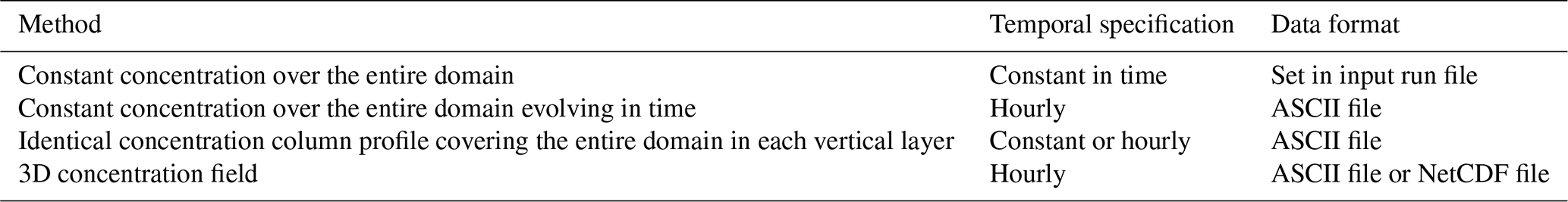
Three options exist (see Table 2) for the specification of pollutant initial and boundary conditions in EPISODE. The first option is to specify a single background concentration at all locations in both the model domain (for initial conditions) and in the grid cells adjoining the model domain. In this case, concentrations can be specified to be time-varying on an hourly basis (only recommended in specific instances) or to remain constant in time (only recommended for testing purposes). This option could be used in a situation when only a single background observation station existed near a city in order to create a time series for a pollutant. The time-varying background concentration is specified in an ASCII input file, while the time-invariant concentration is specified in the EPISODE run file.
The second option is to specify a single vertical profile of background concentrations for every grid cell in the horizontal domain and adjoining background grid cells. The vertical profile must have a vertical resolution matching the model's configuration. This can be done so that the profile is defined on an hourly basis or remains constant in time. The latter option is only recommended for testing purposes, but the time-varying option would be appropriate if the background concentrations are defined by a coarse-horizontal-resolution (i.e. >50 km) regional or global CTM. If used, the temporally varying vertical profiles and the constant vertical profile need to be specified in ASCII input files that are referenced in the EPISODE run file. The last option allows for the specification of background concentrations on the 3D-grid of the model. In this case, the concentrations are specified on the same horizontal and vertical grid as the model and the adjoining grid cells outside the model domain in the x, y, and z dimensions. The background concentrations are specified on an hourly basis in NetCDF or ASCII input files. This option in EPISODE gives the opportunity to run EPISODE in a one-way nesting configuration embedded within a regional-scale CTM. So far, this option has been used with three different regional-scale CTMs to provide the fields of pollutant background concentrations. In the first example, outputs from the Copernicus Atmospheric Monitoring Services (CAMS) regional production (Marécal et al., 2015) were interpolated from their 10 km horizontal resolution down to a resolution of 1 km. This configuration has been used in the Nasjonal Beregningsverktøy (NBV) (Tarrasón et al., 2017) and BedreByLuft projects (Denby et al., 2017), which both focused on air quality in Norwegian cities. In the second example, output from the EMEP CTM model (Simpson et al., 2012) was also used in a similar fashion to provide background concentrations. In the third example, the CMAQ model (Byun and Schere, 2006) was used to provide background concentrations with the CMAQ output interpolated from 4 km horizontal resolution down to ∼1 km. CMAQ is used in the example presented in Part 2 of this article (Karl et al., 2019).
Photostationary state scheme
EPISODE has been designed to be used in urban environments at high latitudes. Under conditions that are polluted (in terms of NOx) and that have relatively low levels of sunlight, it is possible to make simplifying assumptions about the photochemistry governing the pollutant NO2.
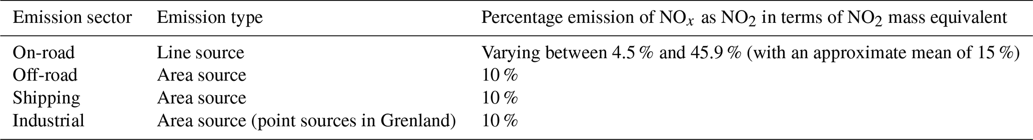
Only a small fraction of NOx emitted from motor vehicles and combustion sources is in the form of NO2 (e.g. with an approximate mean of 15 %), the largest fraction being NO. The majority of ambient NO2 originates from the subsequent chemical oxidation of NO. Under polluted, low-light conditions, the vast majority of this oxidation occurs via reaction with O3 (Reaction R1).
NO2 readily undergoes photolysis via Reaction (R2).
Even at the latitude of Oslo, NO2 can have a lifetime with respect to photolysis on the order of minutes at midday in winter. Reaction (R2) and the subsequent reformation of O3 via Reaction (R3) must therefore be considered if we want to describe NO2 concentrations under these conditions.
Reaction (R3) between the oxygen radical (O(3P)) and molecular oxygen (O2) occurs very rapidly and can be assumed to occur instantaneously. We can then reduce the photochemical system describing NO2, NO, and O3 to the equilibrium reaction described in Reaction (R4):
whereby the forward reaction describes the production of NO2 via Reaction (R1) (reaction coefficient k(O3+NO)), and the backward reaction (rate coefficient described by JNO2) consists of the combined photodissociation of NO2 (via Reaction R2) and the subsequent, assumed, instantaneous formation of O3 (via Reaction R3). The reaction rate for Reaction (R2) is calculated with a parameterisation (Simpson et al., 1993) that uses sun angle and cloud cover to calculate JNO2, which is described by Eq. (S2.2b) within Sect. S2 in the Supplement. We assume that this photochemical mechanism is adequate for polluted Nordic wintertime conditions when net photochemical production of O3 and losses of NOx via nitric acid production are at a minimum. However, when solar ultraviolet (UV) radiation is stronger, in particular during summer months or at more southerly locations, net ozone formation may take place in urban areas at a certain distance from the main emission sources (Baklanov et al., 2007). Please refer to Part 2 of this article (Karl et al., 2019) wherein the EPISODE–CityChem model is described, which uses a more comprehensive photochemical scheme suitable for more sunlit environments.
The PSS approximation is used to resolve the NO2, NO, and O3 photochemistry on the 3D Eulerian grid and at the receptor points for the sub-grid-scale model. The PSS is an analytical mathematical solution that can be applied to Reaction (R4) to estimate the concentrations of NO2, NO, and O3. The PSS has two key assumptions. First, the chemical system is in equilibrium; second, equilibrium is attained instantaneously. These assumptions imply that the residence time of pollutants is much larger than the chemical reaction timescale, and they are valid for polluted urban conditions. Section S2 in the Supplement gives an in-depth explanation of the PSS and how it is applied in this case for Reaction (R4).
Taken together, the PSS and its application to Reaction (R4) are therefore adequate for the Nordic case studies we present in this paper and for the previous and existing applications of the EPISODE model in Norway.
2.2.2 Sub-grid-scale model components
Line- and point-source emissions
We describe here the implementation of the sub-grid-scale emissions in EPISODE. The line-source and point-source emissions are prepared in advance by one of two possible preprocessing utilities. These utilities are described in Sect. 2.4.
For the line sources, these tools prepare two emission files that are defined in the run file and read directly into EPISODE at runtime. The files describe necessary details such as location, road length, and emission source strength. Further details of both files are described in Appendix A. The point-source emissions are used for describing emissions from stacks. The details of each stack are specified in a separate emission file that details the emission source, e.g. stack height and emission rate. Further details are described in Appendix A. EPISODE reads in this information at runtime and calculates the injection heights for the point-source emission using a parameterisation based on Briggs (1969, 1971, 1974, 1975) that considers the processes of stack downwash and buoyancy-driven plume rise under different stability conditions.
The stack downwash process modifies the physical height of the chimney to estimate an effective stack height (Briggs, 1974). Buoyancy-driven plume rise will affect the final plume height in different ways according to the boundary layer stability conditions, and therefore there are different parameterisations for either unstable and neutral conditions or stable conditions. The final injection height is calculated by taking into account the effects of the adjacent building (considering its height and width) on building-induced disturbances of the plume flow, plume penetration through elevated stable layers, and topography. Further details of the parameterisations are described in Sect. S3 of the Supplement.
Line-source Gaussian dispersion
The line-source model is based upon the steady-state integrated Gaussian plume model HIWAY-2 (Petersen, 1980). A fixed rectangular area of influence surrounds each road link that defines the zone within which emissions from line sources are assumed to affect concentrations at receptor points within a single dynamical time step. Figure 2 shows an illustration of the area of influence around an example road link. The boundaries of the distance of influence extend Rinf (the influence distance) from the road link centres perpendicular to the road link direction. In the longitudinal direction, the distance of influence extends Rinf from the two ends of each road link. The area of influence excludes receptor points assumed to be on the road links themselves, which is defined by the distance Rmin (Fig. 2). Rmin is 5 m plus half the road link width.
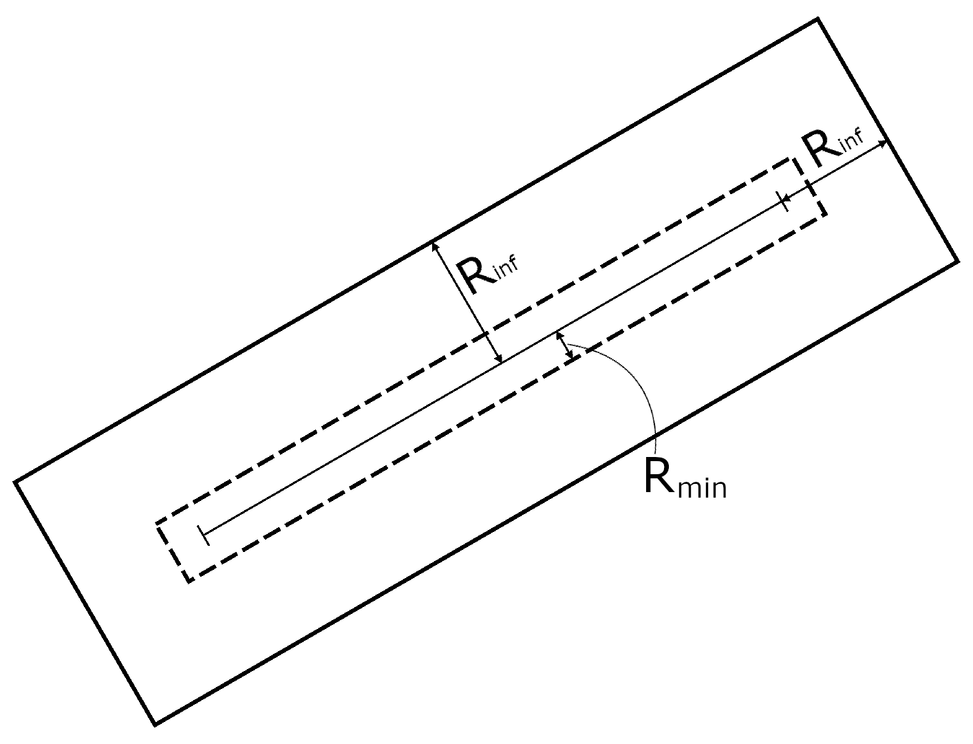
Figure 2An illustration of the rectangular area of influence around an example road link showing the minimum (Rmin) and maximum (Rinf) distances influenced by a line source.
HIWAY-2 resolves the dispersion from the line sources by splitting each road link up into smaller line-source segments and then calculating the dispersion from these segments individually. The line-source segments are of equal length and are spaced equally along the road links. The emission intensities from each segment, El, are calculated as a fraction of the total emission along the road link, ER, according to
where Dl is the length of the line-source segment and DR is the total length of the road link. Therefore, all of the segments emit equal pollutant mass, which is proportional to the fractional length of the road segment Dl∕DR. Note that El is in grams per second (g s−1), whereas ER is in grams per second per metre (g s−1 m−1).
HIWAY-2 only calculates the dispersion from the line sources to each of the receptor points within their respective areas of influence during the last dynamical time step of each hour. Note that EPISODE only outputs pollutant concentrations on an hourly basis. Prior to the last dynamical time step, line-source emissions are only emitted directly into the Eulerian grid (see Sect. 2.2.2). The implicit assumption is that due to the short transport distance, emissions from road links can only affect receptor point concentrations within the distance of influence, Rinf, on short timescales equivalent to a single dynamical time step. The length of the dynamical time step scales with the wind speed such that higher wind speeds result in shorter dynamical time steps. The user can set the Rinf for each road link, but typically a value of 300 m is used. That is the Rinf used in the case study in this paper, which corresponds to a value well below the simulated distance typically travelled by an air mass in a single dynamical time step.
The line-source dispersion model is described in further detail in Sect. S4 of the Supplement.
Point-source Gaussian dispersion
Two point-source plume parameterisations have been implemented in EPISODE to represent dispersion from chimney stacks. The first scheme is a Gaussian segmented plume model called SEGPLU (Walker and Grønskei, 1992) following the general method described by Irwin (1983). The second scheme is a puff model called INPUFF (Petersen and Lavdas, 1986). Both schemes use point-source emissions and their injection heights calculated following Briggs (1969, 1971, 1974) described earlier in Sects. 2.2.2 and S3 of the Supplement. The emissions from point sources are treated as a sequence of instantaneous releases of a specified pollutant mass that then, in turn, becomes a discrete puff or plume segment. The subsequent position, size, and concentration of each plume segment or puff is then calculated in time by the model during each dynamical time step. This information is used to calculate a plume segment's or puff's contribution to the receptor point surface concentrations during the last dynamical time step of each hour.
Plume segments and puffs stop being traced during any dynamical time step in the following cases: (1) they move outside the model domain; (2) they become too large; (3) they encounter a large change in wind direction causing them to become spatially separated. If the segments or puffs become too large or are separated whilst within the model domain, the pollutant mass within them is transferred to the grids in which they currently reside during that dynamical time step; otherwise, they are deleted (see Sect. 2.2.2 for more details).
The SEGPLU and INPUFF models are described in further detail in Sects. S5 and S6 of the Supplement, respectively.
Receptor point concentration calculation
The concentrations at receptor points are calculated at the end of each hour by combining the concentrations at the surface layer of the Eulerian grid with the contributions from line and point sources. Up until that time step, the model only calculates the chemistry and transport on the Eulerian grid, while also simultaneously calculating the position and concentration of plume segments and/or puffs. The receptor point concentration at the end of each hour can be described by Eq. (7):
where is the receptor point concentration at receptor point r* at time t, is the Eulerian grid concentration from the penultimate dynamical time step during each hour (for the grid cell where r* is located), is the line-source segment concentration contribution from line-source segment l, and is the point-source concentration contribution from a plume segment or puff, p. To resolve Eq. (7), EPISODE sums up the concentration contributions from the total number of line-source segments, L, within Rinf distance of the receptor point and the total number of point sources P. The Eulerian grid concentration from the penultimate dynamical time step, , is used to prevent double counting because it does not include line- and point-source emission contributions from the final, and current, dynamical time step in the hour. Testing (not shown) demonstrates that using this assumption in combination with an Rinf of 300 m (see Sect. 2.2.2) reliably reduces double counting of emissions to negligible levels. For the simulation of NO2, EPISODE resolves Eq. (7) for both NO and NO2, thus calculating ) for both compounds. Using the Eulerian grid concentration of ozone combined with the NO and NO2 receptor point concentrations, the photochemistry is solved at each receptor point using the PSS to create updated concentrations for NO2, NO, and ozone that are provided as the hourly model outputs.
Interaction between receptor and Eulerian grid concentrations
Until the final dynamical time step of the hour, the emissions from line-source segments are emitted directly into the grid in which they reside during each time step. Each line-source segment in an Eulerian grid cell () makes a contribution to the Eulerian grid concentration, Cm, which can be described as a tendency, , via
where is the volume of the Eulerian grid cell () into which the emissions occur, and dt is the length of the dynamical time step. Since we are discussing line segments within a specific grid cell we use a specific and distinct notation different from that in Eq. (7). Therefore, a line-source segment in a particular grid cell () is denoted as l∗ and the total number of line segments in a grid cell as L∗. In practice, the emissions from road links are emitted directly into the lowest layer of the Eulerian grid. Line segments are sufficiently short in length that each one can emit entirely within a single Eulerian grid cell.
The change in grid concentration, , due to line-source segment contributions is calculated via
In the last dynamical time step of the hour, pollutants from line sources are both emitted directly into the Eulerian grid according to Eq. (8) and are also dispersed to the receptor points according to the descriptions in Sects. 2.2.2 and S4 of the Supplement.
Point-source emissions also contribute to the concentrations at receptor points and the Eulerian grid. Point sources continually emit plume segments or puffs every dynamical time step that are dispersed and advected according to Sect. 2.2.2 and Sects. S5 and S6 of the Supplement. At the end of each hour, plume segments and/or puffs are assessed to see if they co-locate with receptor points at the surface; in this case, they contribute to the receptor point concentrations via Eq. (7). In the case that plume segments or puffs become invalid, they will be deleted, and the pollutant mass within them, mp, will be added to the concentration of the grid cell in which they reside as a tendency specific to that plume segment or puff, . This tendency is calculated via
and the change in grid concentration, ΔCm,p, resulting from the deleted plume segment or puff mass is calculated via
2.3 Meteorological inputs
The meteorological inputs can be provided by a separate NWP, from The Air Pollution Model (TAPM), or from an observationally driven diagnostic model called MCWIND. These different meteorological inputs drive the transport processes at both the grid and sub-grid scales.
The Applications of Research to Operations at Mesoscale (AROME) (Bengtsson et al., 2017) and Weather Research and Forecasting (WRF) (Skamarock et al., 2019) NWP models have both been used to provide inputs for EPISODE. In the case of AROME, we access the Norwegian Meteorological Institute's THREDDS server (https://thredds.met.no/thredds/catalog.html, last access: 7 April 2020) to retrieve the data that are needed. We run the WRF model for the specific cases we study for situations when AROME data are not available. TAPM (Hurley, 2008; Hurley et al., 2005) is a prognostic meteorological and air pollution model that can be used to create meteorological input for EPISODE; please consult Part 2 of this paper for more details on TAPM and an example of its application (Karl et al., 2019).
The MCWIND utility produces a diagnostic wind field and other meteorological fields for the defined model grid by first constructing an initial first-guess wind field based on the measurements of the horizontal wind and vertical temperature differential at two or more meteorological stations. Then the horizontal 2D fields are interpolated to the 3D grid of the model domain by applying Monin–Obukhov similarity theory. Finally, the first-guess 3D wind field is adjusted to the given topography by requiring the resulting wind field in each model layer to be non-divergent and mass-consistent.
The meteorological inputs have to be provided on the 3D spatial gridding used by the EPISODE model, which is defined in the EPISODE input run file. Thus, in the case of AROME, WRF, TAPM, and MCWIND, these external models and utilities have to be run at the same spatial resolution as the planned EPISODE simulations. In most applications EPISODE is run at 1 km×1 km horizontal resolution but has been run at 200 m×200 m resolution. The typical vertical resolution used is such that the layer adjacent to the surface is 24 m thick, there are 20 layers within the first kilometre, 8 layers between 1 and 2 km in altitude, and a further 7 beyond that up to 3.5 km. The meteorological inputs are typically provided at hourly intervals and have been done so for all current and recent applications. However, the interval can be set to different times depending on the limitations of the input meteorological data.
2.4 Preprocessing utilities
Several preprocessing utilities are used in conjunction with the EPISODE model. These utilities are used for preparing meteorological inputs, emissions files, and boundary condition files used in the running of an EPISODE simulation. The preprocessing utilities are as follows:
-
CAMSBC (collection of routines to convert CAMS regional production to EPISODE background input) – the CAMS regional data can be used as background pollutant concentrations and can be downloaded directly from the CAMS online data portal (CAMS online data portal: https://atmosphere.copernicus.eu/data, last access: 7 April 2020);
-
UECT (interface for line-source, point-source, and area-source emissions; allows the use of EPISODE independent of AirQUIS);
-
TAPM4CC (interface to convert TAPM meteorology output when TAPM is used as a source of meteorological input); and
-
utilities to generate auxiliary input.
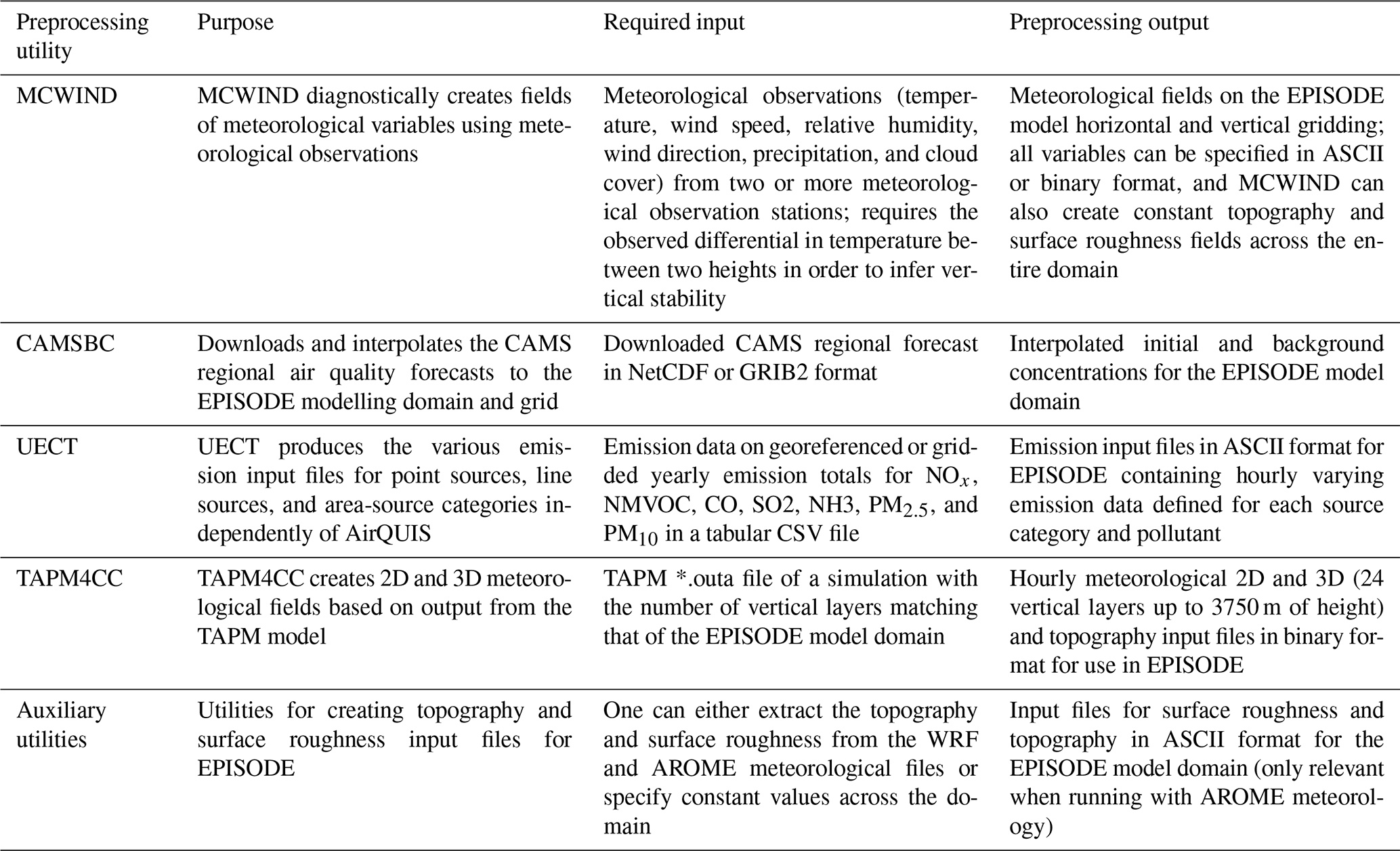
Table 3 gives an overview of the purpose of the preprocessing utilities as well as outlining the input and output formats and descriptions.
Table 3Description of the preprocessing utilities used for preparing input files for the EPISODE model.
As a demonstration and validation of EPISODE's capabilities we carry out simulations of NO2 concentration levels over six Norwegian cities. The chosen urban areas are Oslo, Trondheim, Stavanger, Drammen, Grenland (including the city of Skien), and Nedre Glomma (encompassing both Fredrikstad and Sarpsborg on the Glomma river). The model domains for these urban areas are shown in Fig. 3. The EPISODE model is run for the entire year of 2015 using meteorological input from the AROME model, which was run operationally over the six city domains by the Norwegian Meteorological Institute (Denby and Süld, 2016). The AROME model simulations are carried out at 1 km×1 km horizontal spatial resolution on the exact same gridding and domain as the EPISODE model simulations for each city. The AROME meteorological outputs are provided every hour and are read into EPISODE at the same frequency. Further details of the meteorological fields used in EPISODE are documented in Sect. S7 of the Supplement. AROME provides NetCDF files for input, and the surface roughness and topography used in AROME were extracted from these files.
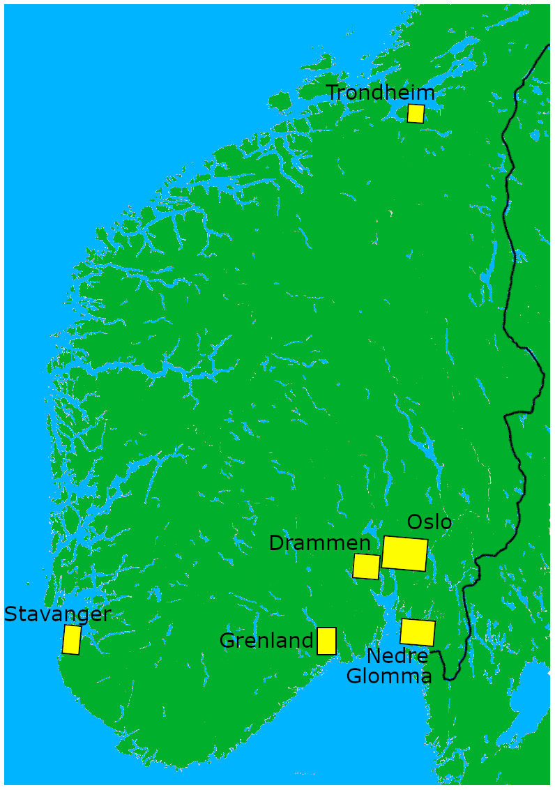
Figure 3A map of the southern part of Norway showing the location and extent of the six modelling domains Stavanger, Trondheim, Grenland, Drammen, Oslo, and Nedre Glomma.
The NOx emissions used for the simulations for each of the six city domains were developed as part of the NBV project (Tarrasón et al., 2017). The methodologies for the creation of the emission datasets are described in Lopez-Aparicio and Vo (2015). The data sources, methodology, and emission reference years are summarised in Table 4 for each sector.
Table 4A description of the data sources, the methodology used, and the reference years for the emission inventories for each emission sector used in the case studies. NRA: Norwegian Road Administration. OFV: Opplysningsrådet for Veitrafikken. HBEFA: Handbook Emission Factors for Road Transport. NCA: Norwegian Coastal Administration. NPRTR: Norwegian Pollutant Release and Transfer Registers.
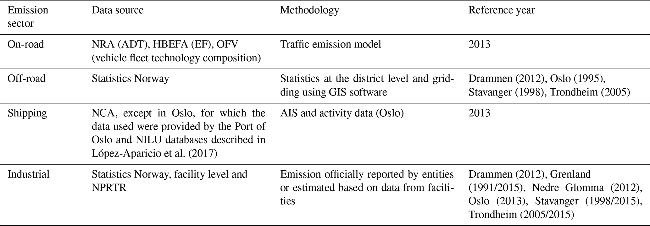
Different approaches were used to compile the emission datasets depending on the data availability for the specific emission sector. On-road traffic emissions are estimated based on a bottom-up traffic emission model. The traffic emission model produces emissions for each road link. It takes into account traffic volume (i.e. average daily traffic, ADT) and the heavy-duty fraction of traffic on specific road types (e.g. highway, city street). In addition, the emission model considers the road slope. This information is obtained from the Norwegian Road Administration. The ADT is combined with temporal profiles of daily traffic to obtain hourly ADT at the road level. The vehicle fleet composition is defined as a fraction of each vehicle technology class (EURO standard) and fuel type, which, combined with the HBEFA emission factors and the hourly fraction of ADT, results in emissions on each road segment. The information regarding the vehicle technology class is obtained from regional statistics (Opplysningsrådet for Veitrafikken, 2013).
Emissions from non-road mobile machinery in construction, industry, and agriculture were originally produced by Statistics Norway, spatially distributed at the district level and thereafter gridded at 1 km×1 km resolution. The previous data stem from different years in each model domain: Drammen from 2012, Oslo from 1995, Stavanger from 1998, and Trondheim from 2005. Non-road mobile machinery is not available in Grenland and Nedre Glomma.
For all cities except Oslo, emissions from shipping are obtained from the Norwegian Coastal Administration based upon the automatic identification system (AIS) following the methodology of Winther et al. (2014). In the case of Oslo, emissions were estimated following a bottom-up approach based on the port activity registering system (López-Aparicio et al., 2017). This includes detailed information on arrivals, departures, and operating times for individual vessels. Industrial emissions were originally provided by Statistics Norway. Industrial emissions are usually linked to the geographical position of large point sources. In the case of Grenland and Nedre Glomma sufficient information (i.e. emission rate, location, stack height and diameter, flue gas speed, and plume temperature) on industrial point sources existed to be able to represent these pollution sources as point sources and to calculate their buoyancy-driven plume rise. However, when achieving this level of detail this was not possible for industrial sources, as in the case for Oslo, Stavanger, Trondheim, and Drammen, they were distributed spatially based on surrogate data, e.g. employment figures in the industrial sector. Finally, for some locations (e.g. Grenland; Table 4), the original dataset of industrial emissions was outdated. In this case, emissions were evaluated and updated based on information from the Norwegian Pollutant Release and Transfer Register.
Table 5 describes how each sector is represented by the different possible emission types, e.g. line or area sources, and presents the ratios between NO and NO2 for the NOx emissions. The fraction of NO2 in emitted NOx (as NO2 mass equivalent) varies between 4.5 % and 45.9 % depending on the source.
Table 5A description of the emission type and the percentage emission of NOx as NO2 (as NO2 mass equivalent) for each sector considered in the model simulation case studies.
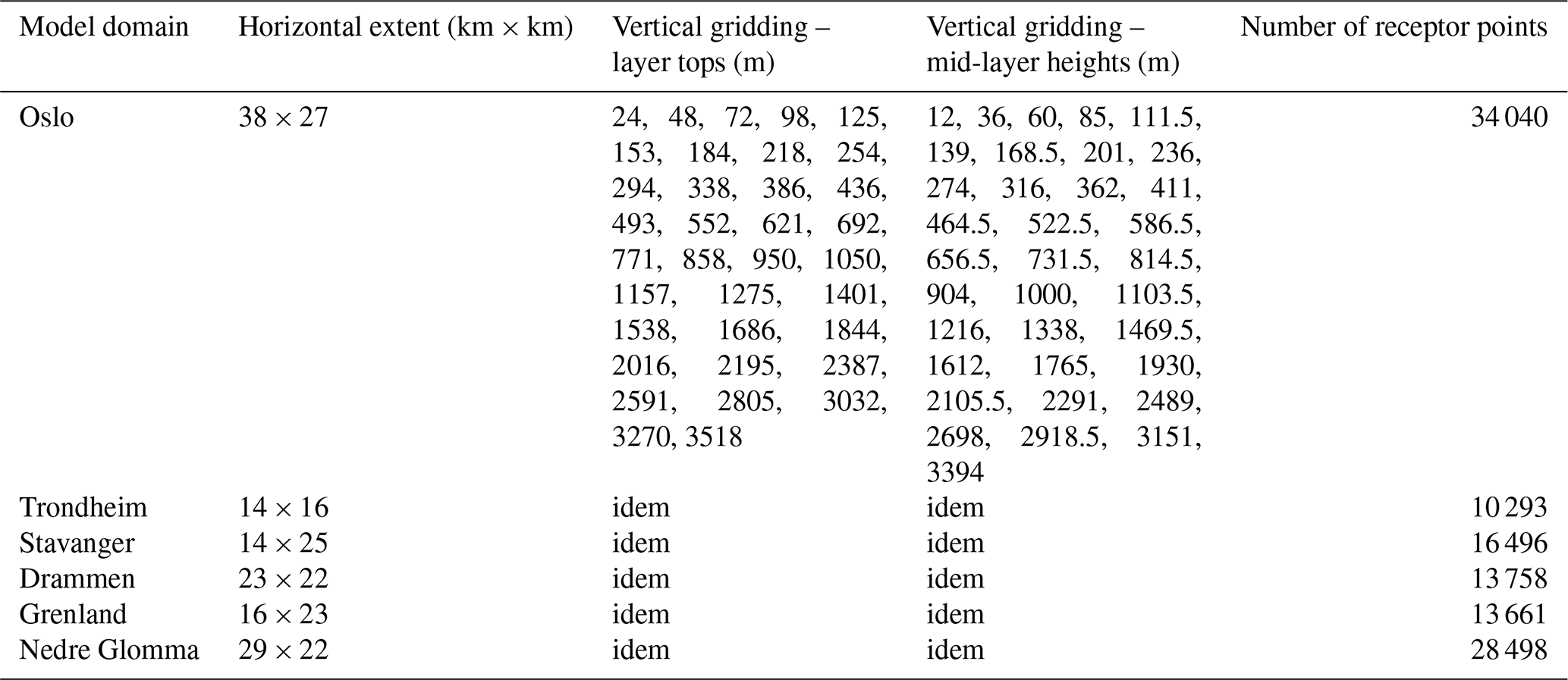
The initial and background hourly concentrations used in the simulations are obtained from the CAMS regional air quality forecast production system (Marécal et al., 2015). The NetCDF files containing NO, NO2, and ozone for a domain covering all of Norway and all vertical levels (0, 50, 250, 500, 1000, 2000, 3000, and 5000 m) came from the CAMS online data portal: https://atmosphere.copernicus.eu/data (last access: 7 April 2020). The CAMS regional forecast data are selected for each city domain and then interpolated horizontally and vertically to the gridding used in EPISODE. In this case study, we used the 34 vertical levels shown in Table 6. Table 6 also gives information on the size of each model domain and the number of receptor points used.
Table 6A description of the horizontal extent, vertical gridding (shown as the height at the top and at the mid-level of each layer, with the mid-level points shown in brackets), and number of receptor points for each model domain. Note that identical vertical gridding was used for all six cities.
4.1 Mapping and evaluation of annual and seasonal model results
4.1.1 Annual mean concentration mapping
Annual mean NO2 concentrations are relevant for air quality mapping since the 2008/50/EC directive (AQD) defines an annual mean NO2 concentration limit value of 40 µg m−3. We therefore present annual mean NO2 concentration maps for four out of the six model domains as a demonstration of EPISODE's application: Oslo (Fig. 4), Drammen (Fig. 5), Nedre Glomma (Fig. 6), and Grenland (Fig. 7). The four selected cities represent the general features that we see in each domain, cover all of the types of simulated spatial variability, and therefore provide a representative sample of the whole.
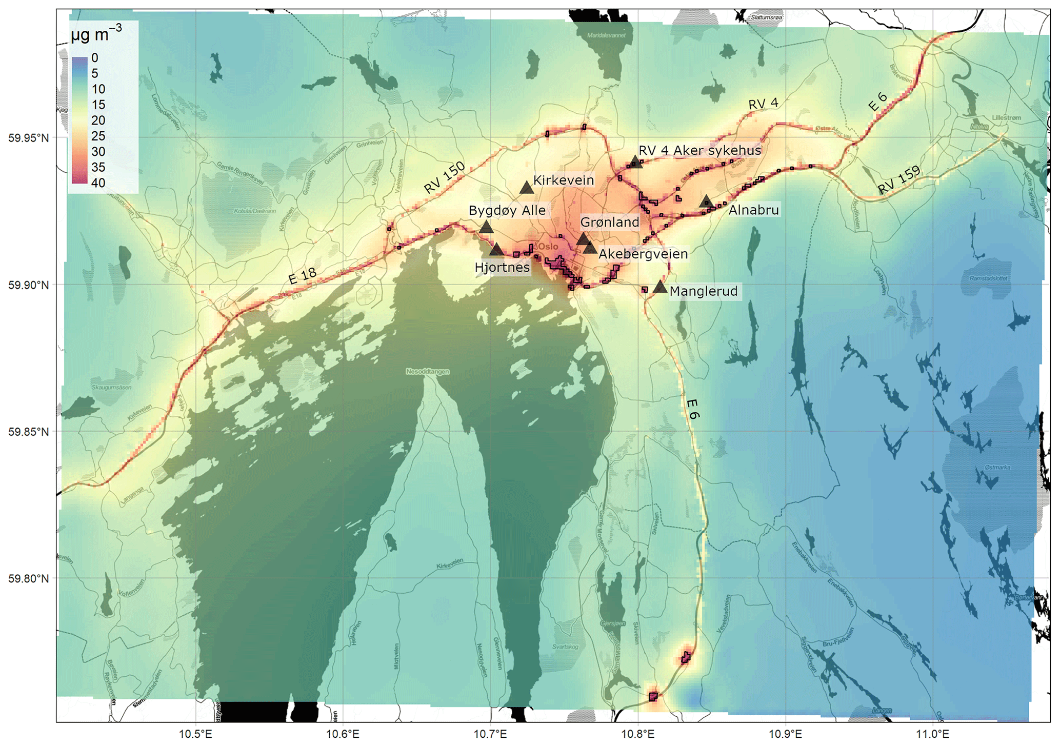
Figure 4Annually averaged NO2 concentrations (µg m−3) from the EPISODE model over the Oslo domain at 100 m×100 m horizontal resolution. The concentrations are derived from the receptor point concentrations and then re-gridded onto a 100 m grid. The colour scale shows the range in annual mean NO2 concentrations between 0 and 40 µg m−3. The black triangles indicate the locations of the air quality observation stations (Table 7). The dark shaded areas represent the sea, lakes, and rivers. The black lines are roads. © OpenStreetMap contributors 2019. Distributed under a Creative Commons BY-SA License.

Figure 5Annually averaged NO2 concentrations (µg m−3) from the EPISODE model over the Drammen domain at 100 m×100 m horizontal resolution. The concentrations are derived from the receptor point concentrations and then re-gridded onto a 100 m grid. The colour scale shows the range in annual mean NO2 concentrations between 0 and 40 µg m−3. The black triangles indicate the locations of the air quality observation stations (Table 7). The dark shaded areas represent the sea, lakes, and rivers. The black lines are roads. © OpenStreetMap contributors 2019. Distributed under a Creative Commons BY-SA License.

Figure 6Annually averaged NO2 concentrations (µg m−3) from the EPISODE model over the Nedre Glomma domain at 100 m×100 m horizontal resolution. The concentrations are derived from the receptor point concentrations and then re-gridded onto a 100 m grid. The colour scale shows the range in annual mean NO2 concentrations between 0 and 40 µg m−3. The black triangles indicate the locations of the air quality observation stations (Table 7). The dark shaded areas represent the sea, lakes, and rivers. The black lines are roads. © OpenStreetMap contributors 2019. Distributed under a Creative Commons BY-SA License.
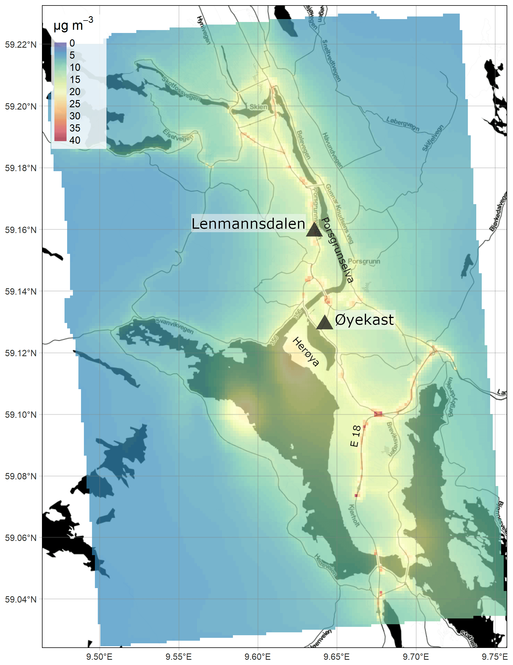
Figure 7Annually averaged NO2 concentrations (µg m−3) from the EPISODE model over the Grenland domain at 100 m×100 m horizontal resolution. The concentrations are derived from the receptor point concentrations and then re-gridded onto a 100 m grid. The colour scale shows the range in annual mean NO2 concentrations between 0 and 40 µg m−3. The black triangles indicate the locations of the air quality observation stations (Table 7). The dark shaded areas represent the sea, lakes, and rivers. The black lines are roads. © OpenStreetMap contributors 2019. Distributed under a Creative Commons BY-SA License.
A primary aim behind the development of EPISODE was to create a model capable of mapping air pollution at high spatial resolution at scales relevant for human exposure within urban areas. We apply a post-processing methodology (outlined in Appendix B: Pollution mapping post-processing methodology) to the irregularly spaced receptor points in order to create pollution maps for each city on a regular 100 m grid. Note that this post-processing method is only applied for visualisation purposes and that for model evaluation (see Sect. 4.1.2) and exposure assessment purposes, the receptor point concentrations (Crec) are used directly.
The most notable features of the spatial patterns present in all of the maps are the elevated concentrations along the principal segments of the road network and main intersections. For example, motorway E18 is visible in the Oslo domain (Fig. 4) running in the east–west direction along the Oslo fjord, in the Drammen domain (Fig. 5) running in the north–south direction on the right side of the map, and in the Grenland domain (Fig. 7) in the southeast corner of the domain. In addition, the E6, another motorway, is visible in Oslo running north–south to the east of the fjord and in Nedre Glomma (Fig. 6) running north–south on the east side of the map. Also visible are district roads like the ones to the east of Oslo (RV4, RV163, and RV159) and road N234 along the north of Drammensfjorden. This reflects the main source for NOx emissions in Norwegian cities: traffic. Oslo has the largest population and largest number of commuters, and this is reflected in the largest hotspot area of concentrations ≥40 µg m−3 of the four presented maps.
Other notable features of elevated NO2 pollution on the maps are what appear to be point-source emissions: in Oslo in the southernmost region of the domain along the E6 (59.74∘ N, 10.82∘ E) (Fig. 5) and in Drammen at 59.738∘ N, 10.16∘ E and 59.73∘ N, 10.22∘ E (Fig. 6). These elevated levels are due to emissions from tunnel mouths. In the Oslo this is the north–south entrances of Nøstvet Tunnel on the E6 and in Drammen the east–west entrances of Strømså Tunnel. The tunnel mouth emissions are prescribed by creating road segments at either end with elevated traffic levels.
Oslo and Drammen are characterised by annual mean suburban NO2 concentrations of 10–20 µg m−3. Oslo, with higher emissions, shows higher background concentrations and a smoother gradient from the city centre to the forested areas with concentrations in the range 0–5 µg m−3. Despite Drammen having similar levels of population as the cities in Nedre Glomma and Grenland, it still shows some relatively high NO2 concentrations compared to these two domains. This is because Drammen sits on the primary commuting route between Oslo and cities to the west and thus has significant commuting traffic.
Both the Nedre Glomma and Grenland model domains have populations divided into two main agglomerations: Sarpsborg and Fredrikstad in Nedre Glomma and Porsgrunn and Skien in Grenland. This leads to NO2 annual mean concentrations in the city centres and suburban areas lower than either Oslo or Drammen. In Nedre Glomma (Fig. 6) the annual average NO2 concentrations reflect the background outside the urban areas and away from the main roads. The background mean NO2 concentration in this area does not fall below 5 µg m−3 because the rural areas in this domain are actually mostly farmland with many off-road service roads that support farmland. This means there is much greater off-road activity and off-road emission sources in this area compared to the other domains.
One aspect of the Grenland domain is the prevalence of industrial pollution sources. Industry is concentrated on the Herøya peninsula at the mouth of the Posrgrunnselva river (in the centre of the domain) and on the western side of the fjord in the southern half of the domain. Mean annual NO2 concentrations are somewhat elevated in these areas with values ∼25 µg m−3. The industrial emissions are treated as stack emissions injected into model layers tens of metres above the surface due to their plume buoyancy and the stack height. This explains why their impact is seen as a more diffuse zone of pollution around the industrial areas.
4.1.2 Full-year and seasonal model evaluation
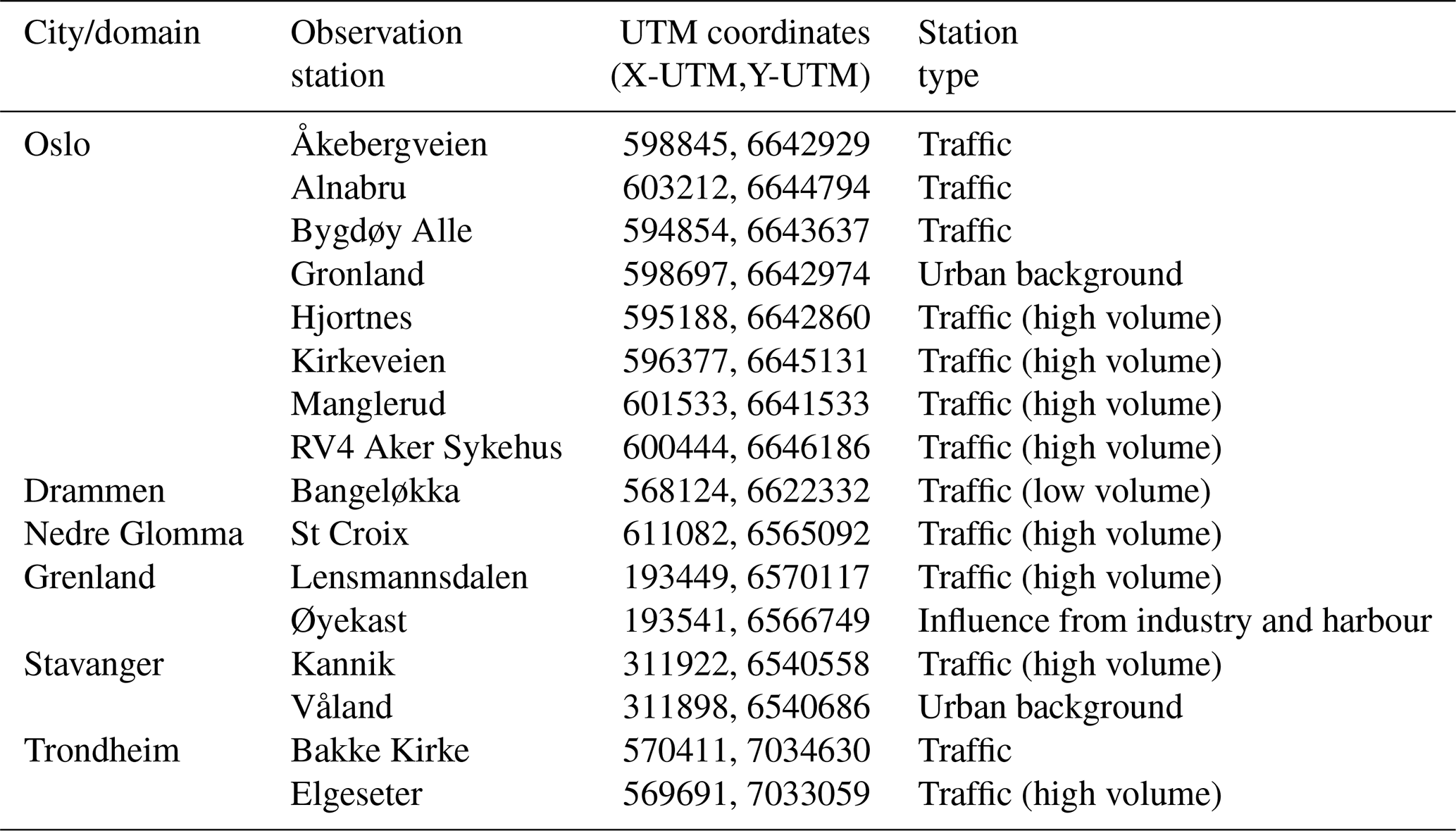
We evaluate the year-long NO2 simulations for 2015 for all six domains (Oslo, Drammen, Grenland, Nedre Glomma, Stavanger, and Trondheim) using in situ air quality observations of NO2. Both the model and observation data will be evaluated in hourly format unless otherwise stated. Due to its size and population Oslo has an increased regulatory requirement to monitor its pollution, and it is therefore the most well-sampled city with a total of eight in situ measurement sites compared to only two at most in the other domains. A receptor point is placed at the coordinate and height of each in situ station shown in Table 7. The simulated concentrations at these receptor points are then used in the evaluation.
Table 7Observation stations used in the evaluation of the EPISODE model results for the six different city domains. The location of each station is shown in UTM coordinates along with the corresponding UTM grid.
We present Taylor diagrams to evaluate the model results compared to the in situ observations. Taylor diagrams visually represent the results of three statistical tests (Pearson correlation coefficient, the root mean square error, and the ratio of the model standard deviation to the observed standard deviation) in a simultaneous fashion. The Taylor diagrams provide a good overall indication of the model performance purely from a statistical standpoint.
Figure 8 shows the results of the statistical tests for the year-long simulation during 2015. Looking at the σM∕σO ratios, we see in general that the model captures the amplitude of NO2 concentration variability reasonably well across all but one of the stations (Våland) with a range in σM∕σO from 0.62 to 1.40. There is a tendency of the model to neither overestimate nor underestimate σ, with an almost equal number of stations above and below 1.0. Only Våland (Stavanger) shows a high spread in modelled NO2 concentrations compared to the observations, with a σM∕σO ratio of 1.67. We can rule out the effect of a persistent bias at Våland since the model shows only a small positive bias (+1.64 µg m−3) with respect to these observations. Instead, this overestimate in the dynamic range appears to be linked to an overestimation in the NO2 diurnal variability during summer. It is possible this is due to an error in the emission magnitude and variability local to Våland during summertime. The comparison with the Kannik station, also in Stavanger, supports this notion since it shows a value of σM∕σO much closer to 1.0 than for Våland. All but 1 of the 16 in situ stations score values of R between 0.5 and 0.67, with only Kannik scoring lower than 0.5 at 0.49. The RMSE ranges between 0.77 and 1.18 µg m−3 for 15 out of the 16 stations. Only Våland has a much higher RMSE at 1.45 µg m−3, which is linked to its high σM∕σO ratio. The results of each statistical test for each station are shown in the Taylor diagrams (Figs. 8, 9, and 10) and are summarised in Table 8. The mean values of R, RMSE, and σM∕σO for all 16 stations are 0.6, 0.96, and 1.06 µg m−3, respectively. This characterises the general model performance.

Figure 8A Taylor diagram calculated using the annual hourly time series of NO2 concentrations for all 16 in situ stations used for the model evaluation across all six domains. The symbols are colour-coded according to each model domain: Drammen is red, Oslo is cyan, Trondheim is green, Stavanger is pink, Grenland is dark blue, and Nedre Glomma is orange. The x and y axes both represent the ratio of the model standard deviation to the observed standard deviation in NO2 concentrations for a particular station such that points can be plotted on concentric circles centred on the x and y origin. The correlation is plotted according to the azimuthal angle from the origin represented as a series of straight lines emanating from the x and y origin. Lastly, the RMSE (µg m−3) is also represented for each station according to their linear distance from 1.0 on the x axis.
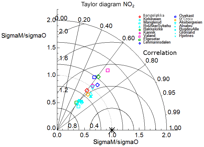
Figure 9A Taylor diagram calculated using the winter-only (January, February, and December) hourly time series of NO2 concentrations for all 16 in situ stations used for the model evaluation across all six domains. The symbols are colour-coded according to each model domain: Drammen is red, Oslo is cyan, Trondheim is green, Stavanger is pink, Grenland is dark blue, and Nedre Glomma is orange. The x and y axes both represent the ratio of the model standard deviation to the observed standard deviation in NO2 concentrations for a particular station such that points can be plotted on concentric circles centred on the x∕y origin. The correlation is plotted according to the azimuthal angle from the origin represented as a series of straight lines emanating from the x∕y origin. Lastly, the RMSE (µg m−3) is also represented for each station according to their linear distance from 1.0 on the x axis.
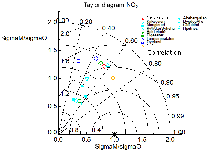
Figure 10A Taylor diagram calculated using the summer-only (June, July, and August) hourly time series of NO2 concentrations for 13 in situ stations used for the model evaluation across five out of the six domains (excluding Stavanger). The symbols are colour-coded according to each model domain: Drammen is red, Oslo is cyan, Trondheim is green, Stavanger is pink, Grenland is dark blue, and Nedre Glomma is orange. The x and y axes both represent the ratio of the model standard deviation to the observed standard deviation in NO2 concentrations for a particular station such that points can be plotted on concentric circles centred on the x∕y origin. The correlation is plotted according to the azimuthal angle from the origin represented as a series of straight lines emanating from the x∕y origin. Lastly, the RMSE (µg m−3) is also represented for each station according to their linear distance from 1.0 on the x axis.
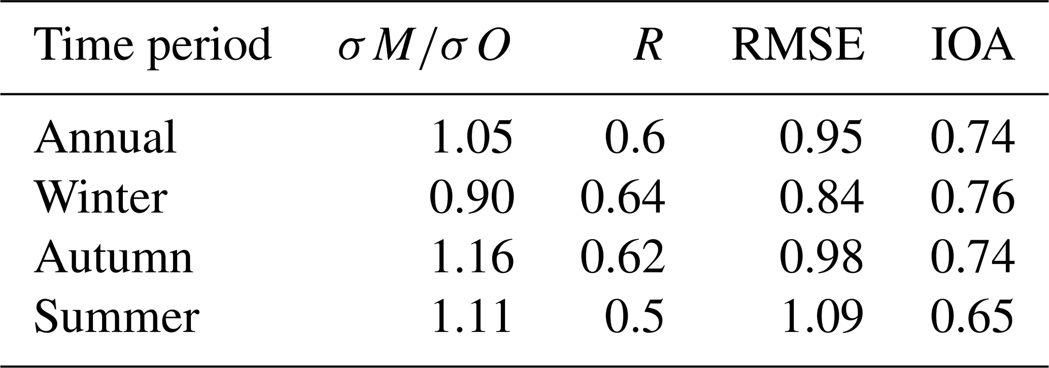
Table 8Mean statistics presented in the Taylor diagram for all 16 observation stations for the full year and the winter, autumn, and summer seasons. σM∕σO is the ratio of the model and observed standard deviation in NO2 concentrations, R is the Pearson correlation coefficient, RMSE is the root mean squared error (µg m−3), and IOA is the index of agreement. These statistical metrics are explained in further detail in Appendix C.
We next evaluate the EPISODE model simulations using only data from the wintertime (January, February, and December combined). We carry out this specific evaluation in order to test the EPISODE model under conditions in which the PSS approximation is likely fulfilled. The PSS is expected to be a reasonable approximation for conditions lacking local photochemical ozone production such as during winter in Nordic environments. Figure 9 shows the results of this evaluation in a Taylor diagram. Evaluating the model solely during winter conditions leads to a substantial improvement in model performance scores. Now 14 out of 16 in situ stations have R values above 0.6, peaking up to 0.69. Only the stations Elgeseter (Trondheim) and Øyekast (Grenland) score below 0.6, both with values of 0.58. Excluding Våland (Stavanger), which has a σM∕σO ratio of 1.42, the σM∕σO ratios range between 0.54 and 1.23 for the remaining stations. Please refer to the earlier discussion of Fig. 8 regarding the high modelled NO2 concentration variability at Våland. Compared to the evaluation of the annual results, the wintertime results show lower values of σM∕σO and a tendency of the model to underestimate the standard deviation of the NO2 concentrations. The temporal variability (not shown) indicates that the stations with the lowest σM∕σO, i.e. Manglerud, Kirkeveien, Bygdøy Alle, Hjortnes, and Alnabru in Oslo and Elgeseter in Trondheim, all tend to underestimate peak daytime NO2 concentrations. The RMSE is reduced overall for the 16 stations: the RMSE ranges between 0.74 and 1.00 µg m−3 with only Våland showing and an RMSE of 1.09 µg m−3 for similar reasons as explained earlier. The mean wintertime statistics are shown in Table 8, which demonstrate a notable improvement in performance compared to the annual statistics. We also checked the statistics during the autumn (no figures shown) and see an improved performance during the period 1 September to 30 November (see Table 8) relative to the rest of the year and the summer.
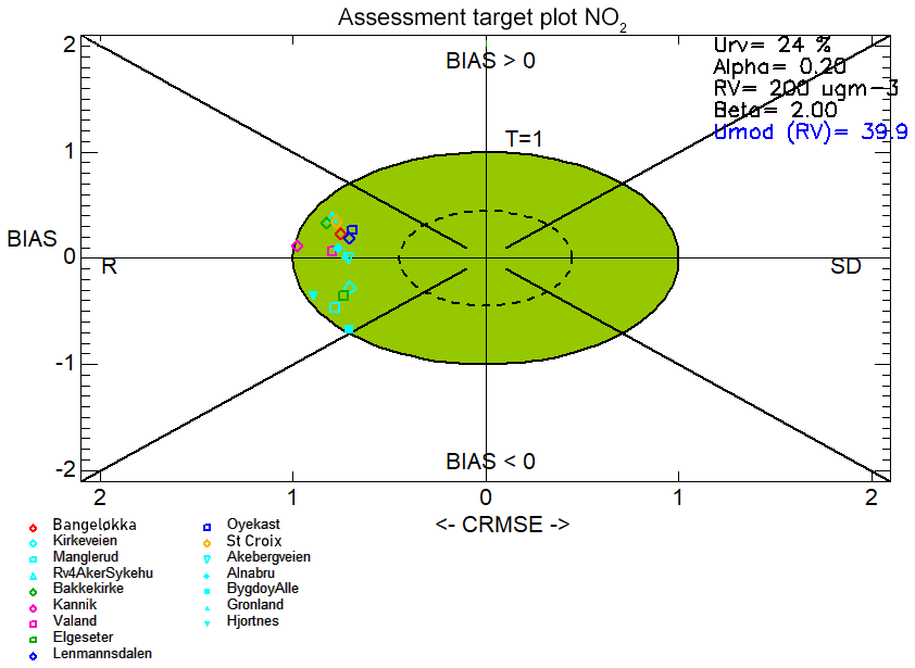
Figure 11Target plots created with hourly time series of NO2 concentrations for 2015 for all 16 in situ stations used for the model evaluation across all six domains. The symbols are colour-coded according to each model domain: Drammen is red, Oslo is cyan, Trondheim is green, Stavanger is pink, Grenland is dark blue, and Nedre Glomma is orange.
The expectation is that the PSS should provide a reasonable approximation of NO2 photochemistry during the winter months. This seems to be supported here by the improved statistics that we see during wintertime compared to the entire year. Furthermore, experiments in Part 2 (Karl et al., 2019) comparing the PSS to the more comprehensive EmChem09 chemical mechanism (70 compounds, 67 thermal reactions, and 25 photolysis reactions) show that it performs adequately within the vicinity of NOx sources. However, despite these encouraging results, the PSS does not include N2O5 formation and subsequent hydrolysis to form HNO3. These reaction pathways are an important sink for NOx during the night (Dentener and Crutzen, 1993), and this is therefore an important limitation of the PSS.
We present evaluation results only for the summertime in the Taylor diagram shown in Fig. 10. We see a notable degradation in model performance in terms of R and RMSE for all stations. In addition, half of the model stations show anomalously high σM∕σO ratio with values of 1.3 or above. We attribute this poorer model performance to the lack of photochemical production of NO2 and ozone represented in the PSS chemistry scheme; without this process we should expect a different diurnal variability in NO2 concentrations from that observed. Even in Oslo, we expect ozone production during the summer months. This is therefore a clear limitation of the PSS, which should have a greater impact in locations further from pollution sources (Karl et al., 2019). Table 8 shows the mean statistics for the 13 stations shown in Fig. 10, and the R and RMSE statistics show an overall degraded performance relative to the annual and wintertime evaluations.
We next evaluate the model performance using the DELTA Tool target plots (Monteiro et al., 2018; Thunis and Cuvelier, 2018; Thunis et al., 2012). These plots offer a means of evaluating different aspects of model performance directly on the axes of the plots, i.e. normalised bias and the centred root mean square error (CRMSE) on the x and y axes, respectively. The DELTA Tool plots also offer a means to evaluate the model within the context of the EC directive while also considering the observation uncertainty. Thus, this type of evaluation offers a different perspective from the statistical measures in the Taylor diagram evaluations. For further details of the DELTA Tool method, consult Appendix C and the references above. The position of a particular model–observation pair (individual points show the results for single stations) in each quadrant reveals which type of error dominates over the other. Specifically, correlation error expressed as R dominates over standard deviation error in the left quadrants, and vice versa in the right quadrants. Meanwhile, points in the upper quadrants indicate positive model bias and the opposite in the lower quadrants. Additionally, the tool uses the CRMSE and normalised bias to calculate a target value, which is also visualised on the target plot as the distance from the origin. The objective is to have points with a target value of 1 or less and thus lie within the green area of the plots.
Figure 12Target plots created using the winter-only (December, January, and February) hourly time series of NO2 concentrations for all 16 in situ stations used for the model evaluation across all six domains. The symbols are colour-coded according to each model domain: Drammen is red, Oslo is cyan, Trondheim is green, Stavanger is pink, Grenland is dark blue, and Nedre Glomma is orange.
Separately, the DELTA Tool calculates the model quality indicator (MQI) (see Appendix C and references therein for further details), which determines whether the model–observation bias is less than the observation uncertainty. Furthermore, Monteiro et al. (2018) and Thunis and Cuvelier (2018) define the model quality objective (MQO) as whether the 90th percentile of MQI for all stations is less than 1. If this criterion is satisfied the model quality objective is satisfied.
Figures 11, 12, and 13 show the target plots for the year-round evaluation, the wintertime-only evaluation, and the summertime-only evaluation, respectively. The target plots highlight an important and consistent feature of the model performance throughout the year, which is that all of the model–observation evaluation pairs lie in the upper and lower left-hand quadrants. This indicates that the correlation error, expressed as R, dominates the contribution to the CRMSE error term.
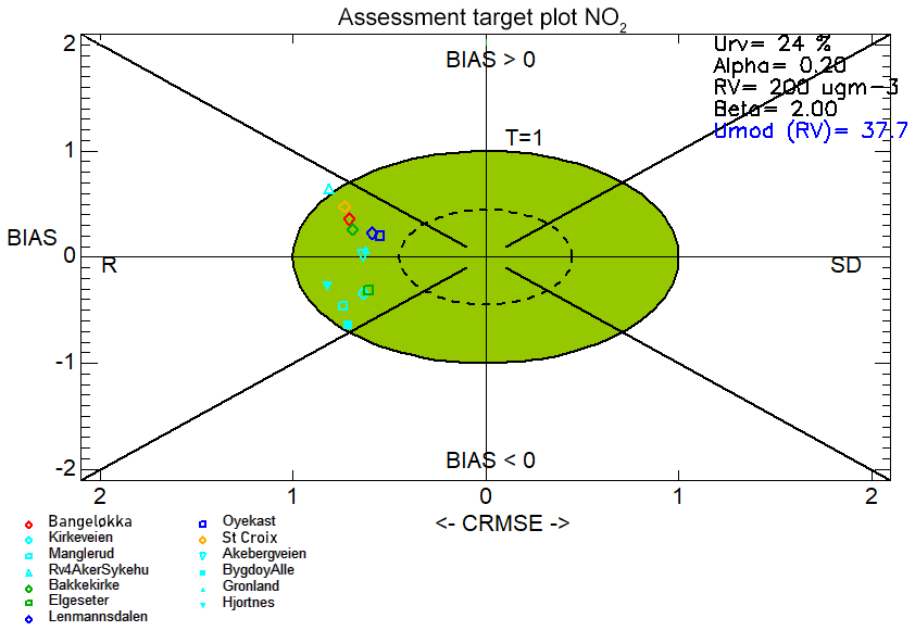
Figure 13Target plots created using the summer-only (June, July, and August) hourly time series of NO2 concentrations for 13 in situ stations used for the model evaluation across five out of the six domains (excluding Stavanger). The symbols are colour-coded according to each model domain: Drammen is red, Oslo is cyan, Trondheim is green, Stavanger is pink, Grenland is dark blue, and Nedre Glomma is orange. Note that there are three missing stations (RV4 Aker Sykehus, Kannik, and Våland) during the summer analysis due to insufficient data.
We first discuss the annual evaluation shown in Fig. 11. The MQO is satisfied for the annual evaluation with the 90th percentile of the MQI calculated at 0.971. Only one station, Bygdøy Alle, has a large enough negative bias to have a specific MQI value above 1. Overall, an equal number of stations have a positive and negative normalised bias. However, there is an apparent signal in the Oslo results for a negative bias in this evaluation, and the magnitude of the negative biases is slightly larger than the positive biases.
EPISODE achieves the MQO during winter with the 90th percentile of MQI being calculated at 0.995. This is despite two stations in Oslo, Åkebergveien and Bygdøy Alle, showing larger than acceptable low biases during the wintertime period. Both stations are visible in the lower left quadrant outside the green target zone. Given the reasonable correlations at both stations, we can perhaps infer that a persistent model or emission process is the cause of this effect. Further study will be required to determine in detail the cause of this, but one possibility is the current lack of a specific consideration of cold-engine starts that have a tendency to increase NOx emissions from vehicle sources during wintertime. Such an explanation would be consistent with the overall bias evaluation in the target plot where we see that there are more stations with a negative bias than a positive bias. Similarly as in Fig. 11, the magnitude of the negative bias is larger than the magnitude of the positive bias, and, similarly, it is the Oslo stations that have a greater tendency to show a negative bias. We note that the MQO is also satisfied during the autumn (figure not shown) with the 90th percentile of the MQI being calculated at 0.996.
Despite the degraded performance shown in the Taylor diagram for the summer in Fig. 10, the MQO is satisfied for the summertime analysis with the 90th percentile MQI being calculated at 0.933. Please note the exclusion of the Kannik and Våland stations due to lack of data. Following guidelines from the EC air quality directive, neither had sufficient observations during the summer to be able to perform the DELTA Tool target plot analysis. Despite this limitation, we can show that the MQO is satisfied across the 13 remaining stations, indicating that the model bias is consistently low enough at these locations on an hour-by-hour basis. The overall bias statistics show no strong prevalence for a negative or positive bias, but, as before, the magnitude of the negative bias is slightly larger and we see a negative bias affecting the Oslo stations in preference to the other cities.
4.2 The model's capability to capture pollution episodes
We now present examples of EPISODE mapping NO2 during pollution events. We select two periods of interest for Oslo and Drammen during which NO2 concentrations became elevated over a few days. The first is an event that took place in Oslo between 9 and 13 December, and the second took place in Drammen between 4 and 7 January. We analyse each event using daily mean maps from the worst day of the pollution event, time series for selected stations, and statistical scores for the available stations.
4.2.1 Oslo pollution episode, 10–13 December 2015
Figure 14 is a plot of the time series for the observed and modelled NO2 concentrations at two measuring sites in Oslo (Åkebergveien and Manglerud) throughout the duration of the event. These two stations are selected because they exhibit different characteristics of the pollution episode with different timings for the onset, and the model exhibits different performance statistics for each station (see Table 9). The pollution event began on 10 December with a period of relatively mild temperatures and moderate southwesterly winds; at this point a peak in NO2 (>60 µg m−3) is only visible at Manglerud (and other stations in the west of Oslo). On the 11 December there was a transition into colder conditions with very light southerly winds that coincided with a worsening of the pollution episode as seen in Fig. 14 at Åkebergveien. The model captures this difference at both stations. Further, the model captures the shorter duration of the peak in NO2 concentrations at Manglerud on 10 December compared to the other days. The cold and light wind conditions persisted for the remainder of the pollution event. For further details on the meteorological conditions for the period 9 to 13 December and for a comparison between the meteorological input to EPISODE and observations, please consult the Supplement Sect. S8.
Table 9Compiled statistics for the comparison between the observed and modelled NO2 concentrations during the 10 to 13 December pollution episode in Oslo. Statistics for each station are shown along with the mean of all of the statistics. σM∕σO is the ratio of the model and observed standard deviation in NO2 concentrations, R is the Pearson correlation coefficient, RMSE is the root mean squared error (µg m−3), and IOA is the index of agreement. These statistical metrics are explained in further detail in Appendix C.
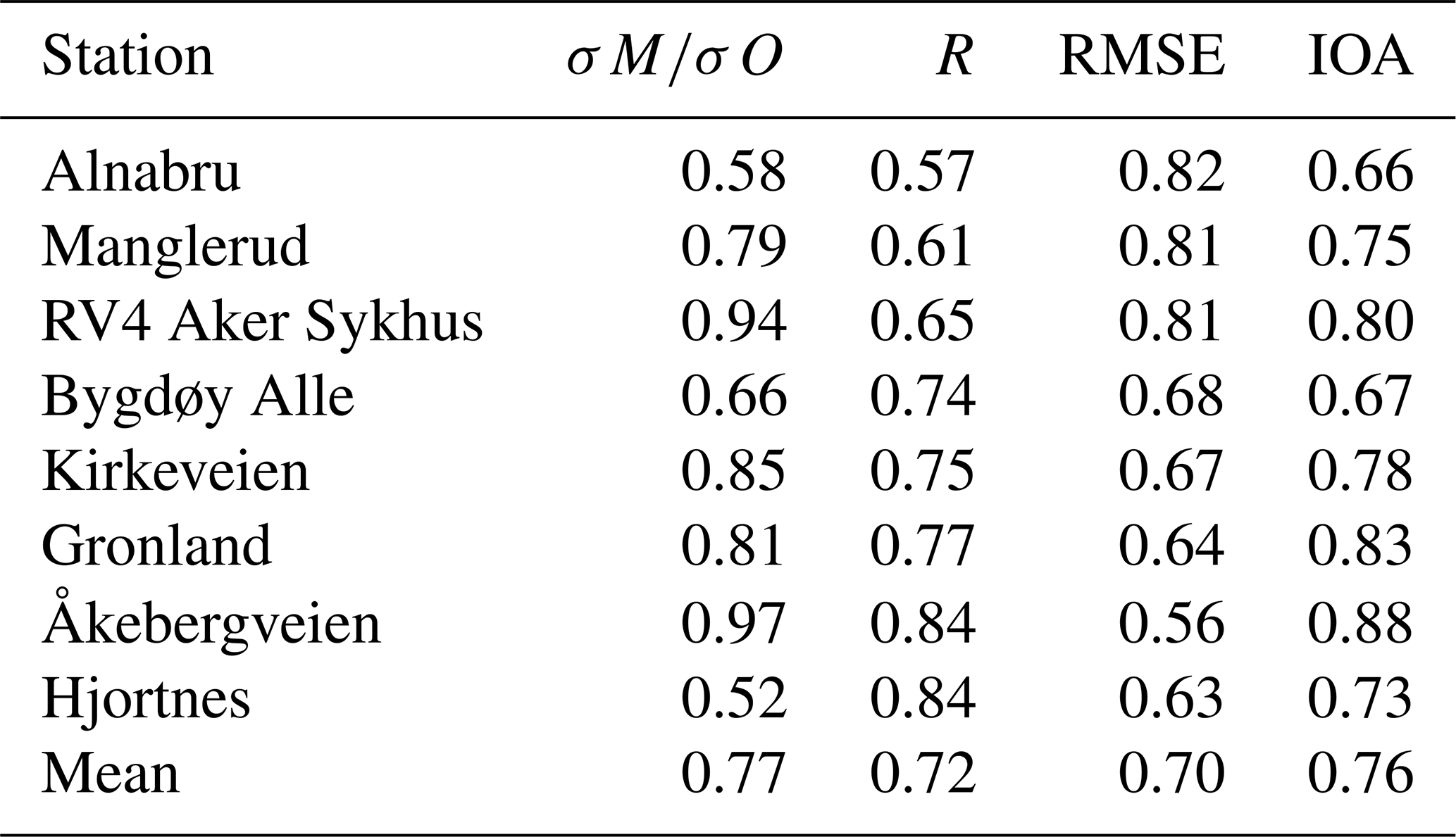
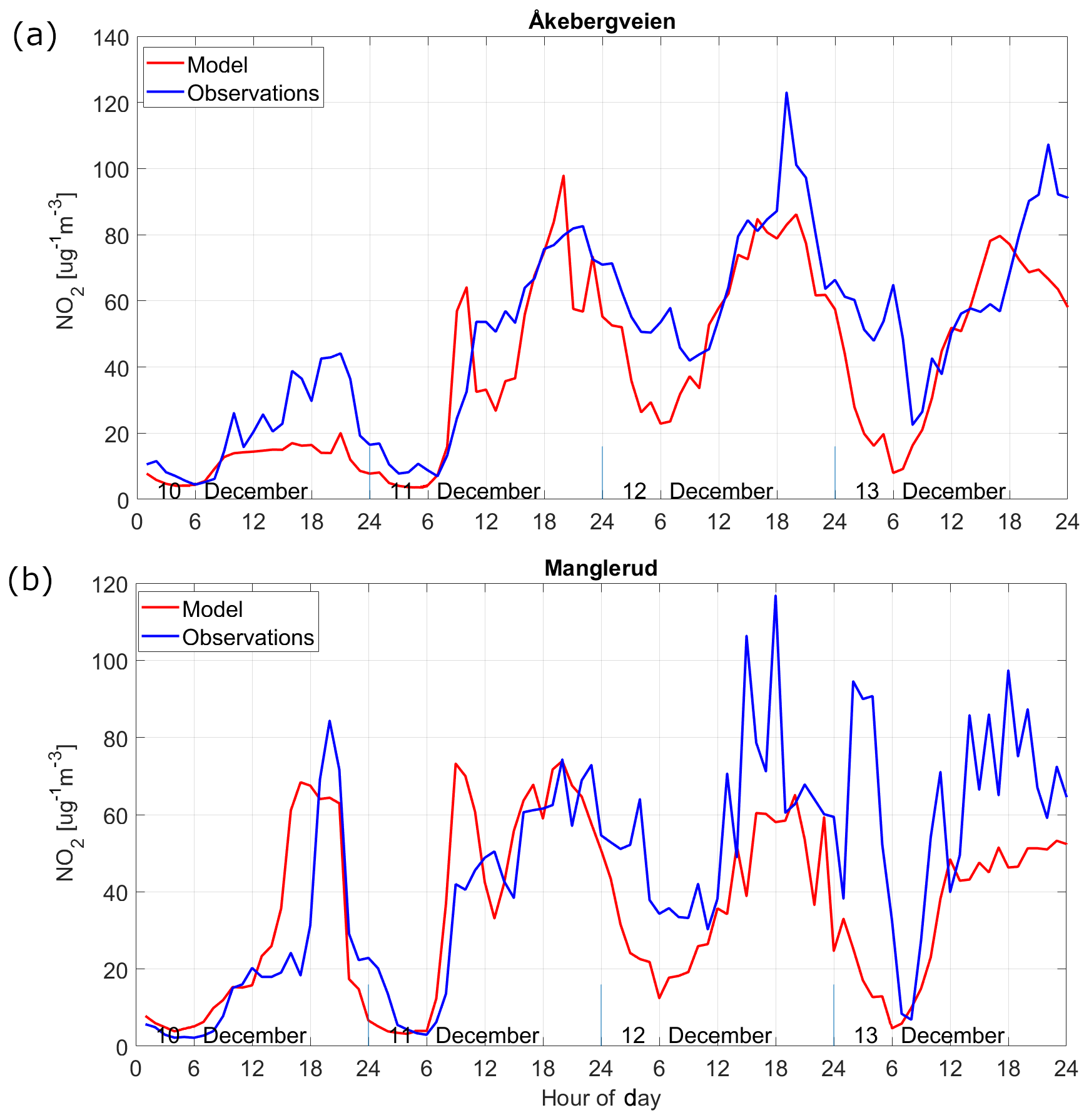
Figure 14Time series of NO2 concentrations for the (a) Åkebergveien and (b) Manglerud measuring stations in Oslo during a pollution episode lasting from 10 to 13 December 2015. Receptor point concentrations from the model are shown in red, and the observed concentrations are shown in blue.
Figure 15 shows a map of the daily mean NO2 concentrations over the Oslo domain for 11 December. The map shows significantly elevated NO2 concentrations over large areas of the domain. Average levels of 40 µg m−3 and higher were present over most of the urban areas in and around the city, with levels of 60 µg m−3 and higher in the central and eastern areas of Oslo and along major roads outside the city. On 11 December the effect of the southerly winds is clearly visible in the form of plumes to the north of roads running east–west to the east of Oslo.

Figure 15Simulated daily mean NO2 concentrations for 11 December from the EPISODE model over the Oslo domain at 100 m×100 m spatial resolution. This day was selected from a pollution episode lasting from 9 until 13 December. The concentrations are derived from the receptor point concentrations and then re-gridded onto a 100 m grid. The colour scale shows the range in annual mean NO2 concentrations between 0 and 60 µg m−3. The black triangles indicate the locations of the air quality observation stations (Table 7). The dark shaded areas represent the sea, lakes, and rivers. The black lines are roads. © OpenStreetMap contributors 2019. Distributed under a Creative Commons BY-SA License.
In Table 9 we can see that the σM∕σO ratio is lower than 1.0 for all comparisons against in situ stations. Looking at Fig. 14 we can see that the model captures the night-time minima reasonably well but underestimates peak NO2 concentrations. This underestimate of the peak is due to uncertainties in boundary layer meteorology, the emissions magnitude, or the time variability of the emissions. Further study will be required to determine the exact cause. Overall, these scores demonstrate acceptable model performance during this pollution episode. This highlights the fact that EPISODE can capture individual pollution events when coupled with meteorological forcing and background pollutant concentrations of sufficient quality.
4.2.2 Drammen pollution episode, 4–7 January 2015
We display the time series of the observed and modelled receptor point NO2 concentrations for Bangeløkka in Fig. 16. Details on the meteorological situation are presented in the Supplement Sect. S8. The onset of the event (>60 µg m−3) started on the afternoon of 4 January during a period of light westerly winds with temperatures close to 0∘C. The pollution worsened (>100 µg m−3) on 5 January during a colder period with very low wind speeds. From 6 January onwards there was no clear wind direction but more moderate wind speeds. Notably, on 6 January the input meteorology overestimates the wind speed, which leads to an underestimate in the peak NO2 concentration that day. Further details on the meteorological situation are presented in the Supplement Sect. S8.
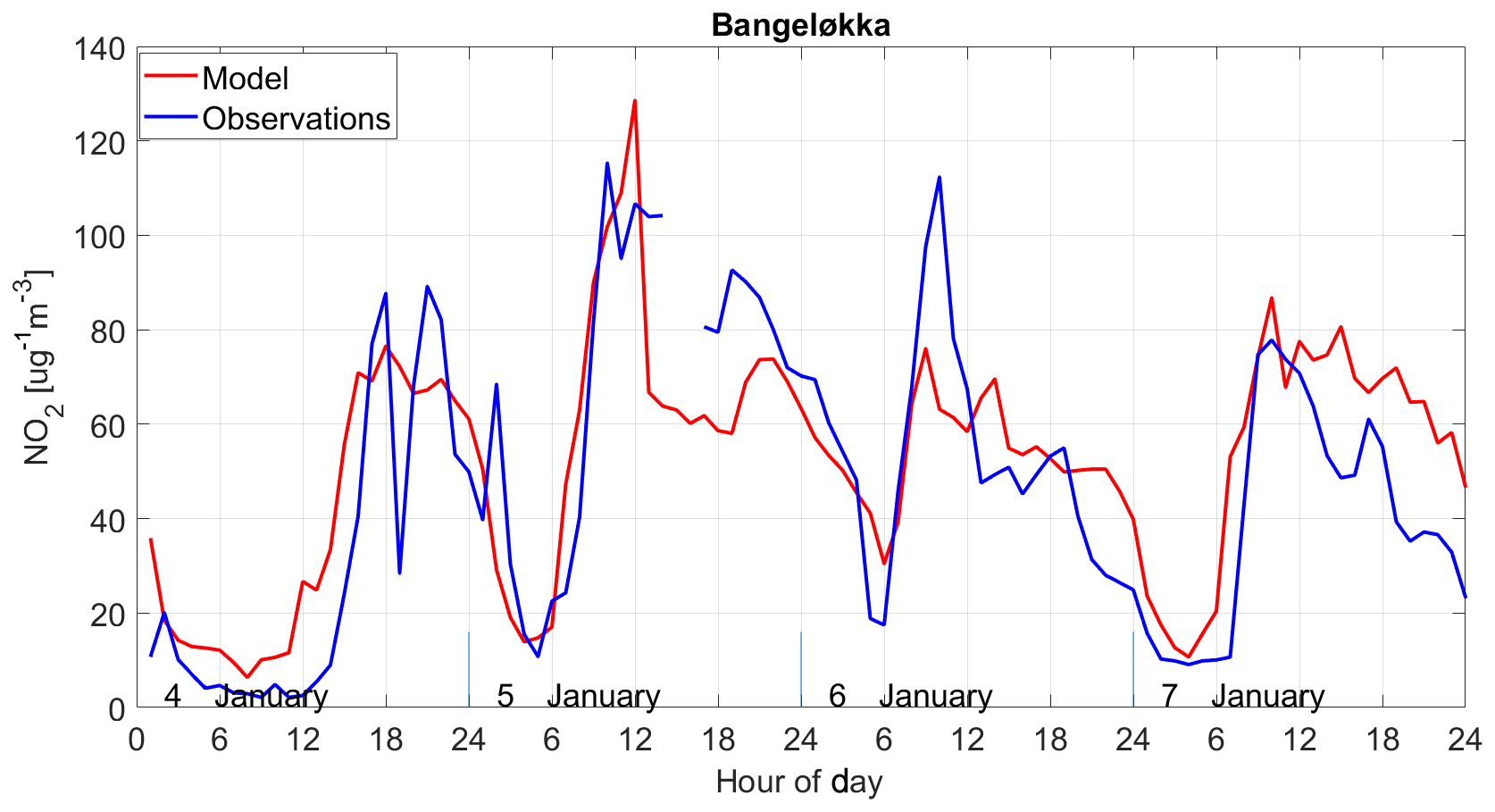
Figure 16Time series of NO2 concentrations for the Bangeløkka measuring station in Drammen during a pollution episode lasting from 4 to 7 January 2015. Receptor point concentrations from the model are shown in red, and the observed concentrations are shown in blue.
Figure 17 shows a map of the mean NO2 concentrations over Drammen for 5 January when the worst pollution occurred. EPISODE simulates concentrations of 30 µg m−3 and higher over much of the populated areas in and around Drammen, along the Drammenselva river, and to the north and south of the fjord along the E18 highway. Only the settlement of Konnerud (in the south-central area of the domain) avoided levels over 30 µg m−3.
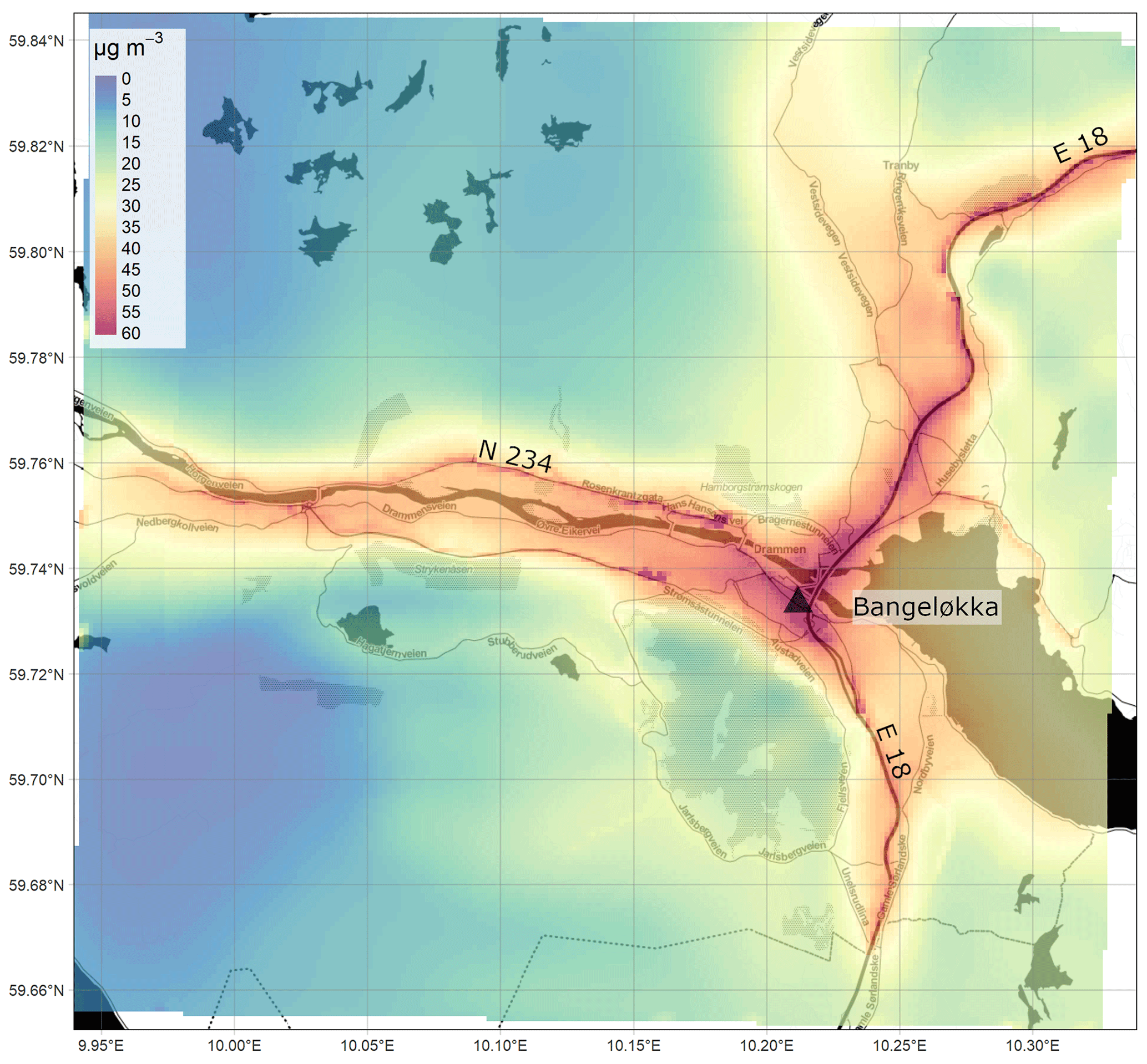
Figure 17Simulated daily mean NO2 concentrations for 5 January from the EPISODE model over the Drammen domain at 100 m×100 m spatial resolution. This day was selected from a pollution episode lasting from 4 until 7 January. The concentrations are derived from the receptor point concentrations and then re-gridded onto a 100 m grid. The colour scale shows the range in annual mean NO2 concentrations between 0 and 60 µg m−3. The black triangles indicate the locations of the air quality observation stations (Table 7). The dark shaded areas represent the sea, lakes, and rivers. The black lines are roads. © OpenStreetMap contributors 2019. Distributed under a Creative Commons BY-SA License.
Evaluating the model performance against the Bangeløkka in situ station in Drammen, we find that the ratio of the modelled and observed standard deviation, σM∕σO, was 0.82, indicating lower than observed model variability. The Pearson correlation R was 0.8, the RMSE was equal to 0.59 µg m−3, and the mean bias was +4.3 µg m−3. The model captures the extent of the night-time minimum in NO2 concentrations (0∕24 to 6 h) on two out of four occasions but does not capture the full extent of the maximum on three out of four days (this is linked to an overestimate of the wind speed on 6 January). Unfortunately, we only have one in situ station available to evaluate the model in the Drammen domain for this pollution episode, which prevents a wider evaluation. Within this limitation, the statistics show acceptable model performance at one of the most polluted sites in Drammen. This again highlights the fact that when coupled with meteorological forcing of acceptable quality and background concentrations of pollutants, EPISODE can capture individual pollution events sufficiently well.
The EPISODE urban dispersion model was presented, which serves as the base model for the EPISODE–CityChem extension described in Part 2 of this paper (Karl et al., 2019). EPISODE combines a 1 km×1 km 3D Eulerian grid with sub-grid-scale dispersion from point and line sources to receptor points. This allows EPISODE to provide a finer-scale and higher-resolution representation of pollution in urban environments than regional chemistry transport models. It thus addresses one of the main weaknesses of regional air quality models, i.e. the recurring problem of representing a diverse range of urban environments (from street-side to urban background) all within a 10+ km scale grid. We presented here the simulation of NO2 pollution at high resolution using a PSS chemistry scheme consisting of NO2, NO, and O3. This scheme was designed to simulate NO2 pollution in Nordic low-sunlight environments for which its usage was considered appropriate. The EPISODE–CityChem extension in Part 2 includes a more comprehensive chemistry scheme suitable for a wider range of environments. We demonstrate the application of EPISODE in six case studies in Norwegian cities for the entire year of 2015. We evaluated the model against in situ observations of NO2 concentrations in all six cities and present more traditional statistical metrics including RMSE, R, and σM∕σO (the ratio of simulated and observed standard deviations), as well as dedicated metrics for evaluating air quality models, e.g. target plot analysis and a model quality objective (Monteiro et al. 2018; Thunis and Cuvelier 2018; Thunis et al., 2012). The model satisfies the model quality objective for every time period it was evaluated for (annual, winter, autumn, and summer), and only 2 stations out of 16 failed the target plot analysis. The statistics over the whole year demonstrate an overall reasonable performance throughout the year. However, more in-depth analysis of the model performance during the different seasons demonstrates significantly improved performance in terms of both correlation and RMSE during autumn and winter compared to summer. The degraded performance of the model during summer is a strong indication of the limitations of the PSS during such conditions. This is consistent with the expectation that the PSS chemistry should perform well during the darker months of the year in polluted environments. The findings in Part 2 of this paper series (Karl et al., 2019) comparing the PSS and EmChem09 chemical mechanisms also support this. Together, these findings demonstrate the suitability of EPISODE for studying the NO2 pollution problem within urban environments in Norway since the most elevated NO2 pollution levels occur during autumn and winter. For this application, we conclude that EPISODE is suitable for the scientific study of NO2 air pollution and also to support policy applications, e.g. NO2 pollution episode analysis, seasonal statistics, policy and planning support, and air quality management.
We outline several developments that are planned in the near future aimed at improving the representation of NO2 in EPISODE simulations. The first is to simulate the entrainment of ozone within NOx-rich plumes from traffic emissions. Currently, the PSS is solved at each receptor point using the NO and NO2 transported from the pollution sources and the grid ozone. We propose replacing the current treatment of ozone and include a simulation of ozone mixing into the NOx-rich plumes linked to the stability conditions.
Another weakness of the PSS is that it solves the chemistry to equilibrium instantaneously regardless of the distance of a receptor point from a pollution source. In reality, the equilibrium between NO2, NO, and ozone may take minutes to achieve. On the short transport timescales of only tens of metres from a pollution source, this may be problematic and a treatment of the chemistry accounting for the time to reach equilibrium and the transport distance may be more appropriate. We plan to modify the PSS calculations to account for this type of situation.
Lastly, we plan to introduce another modification to the photostationary steady state that will simulate the formation of N2O5, which is an important wintertime sink for NOx (Dentener and Crutzen, 1993). This will require the introduction of the chemical species NO3 and N2O5 into the photostationary steady-state scheme. N2O5 loss onto aerosols will be considered via an uptake coefficient onto a dynamically calculated particulate matter surface area derived from the simulation of particulate matter concentrations. We are planning to carry out a comprehensive and focused evaluation of the new urban K(z) method described in Sect. 2.2.1 in a dedicated separate study in the near future. This is dependent on obtaining suitable observations, which we plan on gathering at the earliest opportunity.
It is already possible to simulate particulate matter concentrations for PM2.5 and PM10 with the EPISODE model (in separate simulations from the NO2 runs), but we chose not to present case studies for these pollutants in this paper. Compared to NO2, the current model uncertainties for simulating PM2.5 and PM10 are much more linked to emission processes, i.e. wood burning and road dust resuspension, respectively. Both emission processes require dedicated models external to EPISODE to estimate realistic emissions, which are beyond the scope of this paper. Running without the inclusion of these emission processes results in significantly degraded model performance compared to the NO2 simulations. The stand-alone emission models are the MEDVED model for wood burning emissions (Grythe et al., 2019) and the NORTRIP model for road dust resuspension (Denby et al., 2013). The offline coupling of both emission models into EPISODE for PM simulations is planned and will greatly enhance the model's capability to simulate particulate matter pollution. In addition to this, a stand-alone traffic exhaust emission model is being developed that will replace many of the functionalities of the AirQUIS system.
To further enhance the simulation of PM within the model, we plan to soon implement PM removal processes, i.e. below-cloud wet scavenging and sedimentation. We will also implement size bins for PM, which will improve the representation of PM removal processes that are affected by particle size, e.g. impaction, diffusion, and interception.
To further benchmark the EPISODE model, it would be interesting to perform an intercomparison with other urban-scale air quality models using identical inputs for a particular case study. The evaluation could then be made using a standardised and accepted evaluation method, e.g. DELTA Tool (Monteiro et al., 2018).
A1 Area gridded emissions
The units of the emissions are grams per second (g s−1), and in the case of NO and NOx this is in terms of the mass of NO2 equivalent. The input format for the area-source emissions is ASCII.
A2 Line-source emissions
The line-source emissions are described in two ASCII input files. The first file describes the road links, giving the UTM coordinates of the road link beginning and end points, the width, the height at the beginning and end points, and the area of influence, Rinf, around a road link. The second contains the hourly total emission intensity along each road link, ER (g s−1 m), for each time step of the simulation. Road link emissions are assumed to be evenly distributed along a single road link.
A3 Point-source emissions
The point-source emission files are in ASCII format and contain the following information for each stack: their hourly emission rates (g s−1), the geographical location of the stack in UTM coordinates, the building width and height, the stack height and diameter, the temperature of the plume gas, and the speed at which the plume is expelled from the chimney.
The visualisation in the maps is created by first subtracting from each receptor point concentration, Crec, the Eulerian grid concentration, Cm, for the corresponding grid square in which the receptor point resides, following
which leaves the local concentration residual, Clocal. Next, the Eulerian grid concentration field at 1 km resolution, Cm, is interpolated to the coordinates, (), of each receptor point using a spline method to give Cm,rec, following
Then, both the residual from Eq. (B1) and Cm,rec are added together to determine the receptor point concentration, Crec∗, which now contains both the receptor point and the interpolated Eulerian grid components. Finally, the modified concentrations for all of the irregularly spaced receptor points, Crec∗, are then re-gridded onto a 100 m×100 m grid covering the entire domain using trilinear interpolation.
In practice, there are many areas within the urban centre with receptor point sampling at spatial resolutions higher than 100 m. Thus, 100 m represents a conservative choice for the effective mapping resolution in these important areas. This post-processing step also serves to remove the visual imprint of the 1 km×1 km Eulerian grid (remember that receptor point concentrations are a sum of the Eulerian grid and local contribution following Eq. (7) from the gridded receptor point concentrations).
The model is evaluated with the following statistical metrics: the ratio of the modelled and observed standard deviation (σM∕σO), root mean squared error (RMSE), centred root mean square error (CRMSE), Pearson's correlation coefficient (R), normalised mean bias (NMB), and index of agreement (IOA).
The respective standard deviations of the model and observations are calculated via
The RMSE provides a representation of the magnitude of the error for each hourly model–observation pair and is defined as (RMSE shares the units of the variables being evaluated: µg m−3)
The IOA is defined as
When the IOA is equal to 1 it indicates perfect agreement between the model and observations, and a value of zero indicates no agreement at all.
The CRMSE and normalised mean bias are used in the axes of the DELTA Tool target plots and are calculated as follows:
In addition to these metrics, we also evaluate the model according to the DELTA Tool model quality indicator (MQI) and the related model quality objective (MQO) (Monteiro et al., 2018; Thunis and Cuvelier, 2018). The MQI calculation provides an advanced evaluation of model performance by considering the observation uncertainty on each individual measurement, U95(Oi), which is defined as
where is the relative measurement uncertainty estimated around a reference value, RV, for a given time averaging, e.g. hourly or daily limit values of the air quality directive. α2 is the fraction of the uncertainty around RV, which is non-proportional to the concentration level, and k is the coverage factor that scales the error in order to achieve a specific confidence interval. k is most typically set to 2 in order to achieve a 95 % confidence interval.
The root mean square of the observation error is calculated via
The MQI is then defined as the ratio between the absolute model–observation bias and a quantity proportional to the observation uncertainty via
where β is a scaling set to 2 in the DELTA Tool. In the DELTA Tool target plots, MQI is the distance between the origin and a point on the plot for a given station. The MQO is considered fulfilled when MQI ≤1. Following the air quality directive requirements, the DELTA Tool sets criteria whereby the MQO is defined as being satisfied when the MQI is fulfilled for at least 90 % of the stations. In other words, ranking the station MQIs in ascending order, the inferred 90th percentile must be 1 or lower.
The source code for the EPISODE model version 10 is available under the RPL 1.5 license at https://doi.org/10.5281/zenodo.3244056 (Slørdal et al., 2019). The model compilation requires installation of the GCC/GFortran Fortran90 compiler (version 4.4. or later) and the NetCDF library (version 3.6.0 or later).
Model input datasets are available from the NILU FTP server upon request. These datasets include meteorological, emission, and ancillary input files for the entire year of 2015; output model data for all of the 2015 simulations; and data in the format for the DELTA Tool analysis package.
The supplement related to this article is available online at: https://doi.org/10.5194/gmd-13-4323-2020-supplement.
PDH wrote the main text of the paper, developed a technical description of the model based on an in-depth evaluation of the code, developed the scientific questions, ran the model case studies for the six Norwegian cities, and analysed and evaluated the EPISODE model results presented in this work.
SEW implemented the HIGHWAY-2 line-source dispersion model and the two point-source dispersion models in EPISODE.
GSS supported the scientific design of the six city case studies and made significant developments to the EPISODE code, e.g. the development of coupling with AROME meteorological data.
PS post-processed the EPISODE model results and visualised the results as the maps.
MV post-processed the EPISODE model results and visualised the results as the maps.
DVT prepared the emissions used in the EPISODE model runs.
SAL provided technical and scientific guidance for the preparation of the emissions used in the EPISODE model runs.
MOPR tested the UECT and TAPM4CC preprocessing utilities and assisted with the DELTA Tool.
MK prepared the observation and modelling data into the correct formats for the DELTA Tool, wrote the technical Supplement, and made contributions to the main text.
The authors declare that they have no conflict of interest.
The authors thank NILU for internal funding used to support this work. NILU thanks Leif Håvard Slørdal (retired) for his major contributions to the development of EPISODE. Leif Håvard Slørdal declined co-authorship, but EPISODE exists today due to his dedicated work. Paul D. Hamer wishes to thank Virginie Marécal and Massimo Cassiani for their scientific discussion in support of this article.
This paper was edited by David Topping and reviewed by three anonymous referees.
Baklanov, A., Hänninen, O., Slørdal, L. H., Kukkonen, J., Bjergene, N., Fay, B., Finardi, S., Hoe, S. C., Jantunen, M., Karppinen, A., Rasmussen, A., Skouloudis, A., Sokhi, R. S., Sørensen, J. H., and Ødegaard, V.: Integrated systems for forecasting urban meteorology, air pollution and population exposure, Atmos. Chem. Phys., 7, 855–874, https://doi.org/10.5194/acp-7-855-2007, 2007.
Baldasano, J., Pay, M., Jorba, O., Gassó, S. and Jimenez-Guerrero, P.: An annual assessment of air quality with the CALIOPE modeling system over Spain, Sci. Total Environ., 409, 2163–2178, 2011.
Basu, S. and Porté-Agel, F.: Large-eddy simulation of stably stratified atmospheric boundary layer turbulence: A scale-dependent dynamic modelling approach, J. Atmos. Sci., 63, 2074–2091, 2006.
Beljaars, A. C. M. and Holtslag, A. A. M.: Flux parameterization over land surfaces for atmospheric models, J. Appl. Meteorol., 30, 327–341, 1991
Benavides, J., Snyder, M., Guevara, M., Soret, A., Pérez García-Pando, C., Amato, F., Querol, X., and Jorba, O.: CALIOPE-Urban v1.0: coupling R-LINE with a mesoscale air quality modelling system for urban air quality forecasts over Barcelona city (Spain), Geosci. Model Dev., 12, 2811–2835, https://doi.org/10.5194/gmd-12-2811-2019, 2019.
Bengtsson, L., Andrae, U., Aspelien, T., Batrak, Y., Calvo, J., de Rooy, W., Gleeson, E., Hansen-Sass, B., Homleid, M., Hortal, M., Ivarsson, K.-I., Lenderink, G., Niemelä, S., Nielsen, K. P., Onvlee, J., Rontu, L., Samuelsson, P., Muñoz, D. S., Subias, A., Tijm, S., Toll, V., Yang, X. and Køltzow, M. Ø.: The HARMONIE–AROME Model Configuration in the ALADIN–HIRLAM NWP System, Mon. Weather Rev., 145, 1919–1935, https://doi.org/10.1175/MWR-D-16-0417.1, 2017.
Bott, A.: A Positive Definite Advection Scheme Obtained by Nonlinear Renormalization of the Advective Fluxes, Mon. Weather Rev., 117, 1006–1016, https://doi.org/10.1175/1520-0493(1989)117<1006:APDASO>2.0.CO;2, 1989.
Bott, A.: Monotone Flux Limitation in the Area-preserving Flux-form Advection Algorithm, Mon. Weather Rev., 120, 2592–2602, https://doi.org/10.1175/1520-0493(1992)120<2592:MFLITA>2.0.CO;2, 1992.
Bott, A.: The monotone area-preserving flux-form advection algorithm: reducing the time-splitting error in two-dimentional flow fields, Mon. Weather Rev., 121, 2637–2641, https://doi.org/10.1175/1520-0493(1993)121<2637:TMAPFF>2.0.CO;2, 1993.
Briggs, G. A.: Plume rise, U.S. Atomic Energy Commission, Oak Ridge Tennessee, 1969.
Briggs, G. A.: Some recent analyses of plume rise observation, in: Proceedings of the Second International Clean Air Congress, edited by: Englund, H. M. and Berry, W. T., Academic Press, New York, 1029–1032, 1971.
Briggs, G. A.: Diffusion estimation for small emissions, Environmental research laboratories air resources atmospheric turbulence and diffusion laboratory 1973 annual report, USAEC Rep ATDL-106 Natl. Oceanic Atmos. Admin., Washington, DC, 1974.
Briggs, G. A.: Plume rise predictions, in: Lectures on Air Pollution and Environmental Impact Analysis, edited by: Haugen, D. A., Amer. Meteor. Soc., Boston, MA, 59–111, 1975.
Businger, J. A. and Arya, S. P. S.: Height of the mixed layer in the stably stratified planetary boundary layer, in: Turbulent Diffusion in Environmental Pollution, edited by: Frenkiel, F. N. and Munn, R. E., Adv. Geophys., 18A, Academic Press, New York, 73–92, 1974.
Businger, J. A., Wyngaard, J. C., Izumi, Y. and Bradley, E. F.: Flux-profile relationships in the atmospheric surface layer, J. Atmos. Sci., 28, 181–189, 1971.
Byun, D. and Schere, K. L.: Review of the governing equations, computational algorithms, and other components of the Models-3 Community Multiscale Air Quality (CMAQ) modeling system, Appl. Mech. Rev., 59, 51–77, 2006.
Byun, D. W., Young, J., Pleim, J., Odman, M. T., and Alapaty, K.: Chapter 7, Numerical Transport Algorithms for the Community Multiscale Air Quality (CMAQ) Chemical Transport Model in Generalized Coordinates, in: Science Algorithms of the EPA Models-3 Community Multiscale Air Quality (CMAQ) Modeling System. EPA/600/R-99/030, U.S. Environmental Protection Agency, Office of Research and Development, Washington, DC, 1999.
Denby, B. R. and Süld, J. K.: NBV report on meteorological data for 2015. Deliverable 6, Work package 3 (Met Report, 2016). Oslo: Norwegian Meteorological Institute, ISSN 2387-4201, 2016.
Denby, B. R., Sundvor, I., Johansson, C., Pirjola, L., Ketzel, M., Norman, M., Kupiainen, K., Gustafsson, M., Blomqvist, G., and Omstedt, G.: A coupled road dust and surface moisture model to predict non-exhaust road traffic induced particle emissions (NORTRIP). Part 1: Road dust loading and suspension modelling, Atmos. Environ., 77, 283–300, 2013.
Denby, B. R., Sundvor, I., Høiskar, B. A. K., and Kristensen, A.: Bedre byluft 2016 – Forskningsresultater og utvikling av prognoser for meteorologi og luftkvalitet i norske byer 2016, Norwegian Meteorological Institute, Oslo, 2017.
Dentener, F. J. and Crutzen, P. J.: Reaction of N2O5 on tropospheric aerosols: Impact on the global distributions of NOx, O3, and OH, J. Geophys. Res.-Atmos., 98, 7149–7163, 1993.
EU: Directive 2008/50/EC of the European Parliament and of the Council of 21 May 2008 on ambient air quality and cleaner air for Europe, Off. J. Eur. Communities, 152, 1–43, available at: http://eur-lex.europa.eu/LexUriServ/LexUriServ.do?uri=OJ:L:2008:152:0001:0044:EN:PDF (last access: 11 September 2020), 2008.
Fagerli, H., Tsyro, S., Denby, B. R., Gauss, M., Simpson, D., Wind, P., Benedictow, A., Jonson, J. E., Klein, H., Schulz, M., Griesfeller, J., Aas, W., Hjellbrekke, A., Solberg, S., Platt, S. M., Fiebig, M., Yttri, K. E., Rud, R. O., Mareckova, K., Pinterits, M., Tista, M., Ullrich, B., Posch, M., Imhof, H., Putaud, J., Cavalli, F., Poulain, L., Schlag, P., Heikkinen, L. M., Swietlicki, E., Martinsson, J., Vana, M., Smejkalova, A. H., Kouvarakis, G., and Mihalopoulos, N.: Transboundary particulate matter, photo-oxidants, acidifying and eutrophying components, EMEP Status Report 2017, available at: http://emep.int/publ/reports/2017/EMEP_Status_Report_1_2017.pdf (last access: 11 September 2020), 2017.
Fedra, K. and Haurie, A.: A decision support system for air quality management combining GIS and optimisation techniques, Int. J. Environ. Pollut., 12, 125–146, 1999.
Foley, K. M., Roselle, S. J., Appel, K. W., Bhave, P. V., Pleim, J. E., Otte, T. L., Mathur, R., Sarwar, G., Young, J. O., Gilliam, R. C., Nolte, C. G., Kelly, J. T., Gilliland, A. B., and Bash, J. O.: Incremental testing of the Community Multiscale Air Quality (CMAQ) modeling system version 4.7, Geosci. Model Dev., 3, 205–226, https://doi.org/10.5194/gmd-3-205-2010, 2010.
Franke, J., Hellsten, A., Schlunzen, K. H., and Carissimo, B.: The COST 732 Best Practice Guideline for CFD simulation of flows in the urban environment: a summary, Int. J. Environ. Pollut., 44, 419–427, 2011.
Grythe, H., Lopez-Aparicio, S., Vogt, M., Vo Thanh, D., Hak, C., Halse, A. K., Hamer, P., and Sousa Santos, G.: The MetVed model: development and evaluation of emissions from residential wood combustion at high spatio-temporal resolution in Norway, Atmos. Chem. Phys., 19, 10217–10237, https://doi.org/10.5194/acp-19-10217-2019, 2019.
Hurley P.: TAPM v. 4, Part 1: Technical Description, CSIRO Marine and Atmospheric Research Paper No. 25, 2008.
Hurley, P., Physick, W., and Luhar, A.: TAPM – a practical approach to prognostic meteorological and air pollution modelling, Environ. Modell. Softw., 20, 737–752, https://doi.org/10.1016/j.envsoft.2004.04.006, 2005.
Irwin, J. S.: Estimating Plume Dispersion-A Comparison of Several Sigma Schemes, J. Clim. Appl. Meteorol., 22, 92–114, https://doi.org/10.1175/1520-0450(1983)022<0092:EPDACO>2.0.CO;2, 1983.
Jensen, S. S., Berkowicz, R., Sten Hansen, H., and Hertel, O.: A Danish decision-support GIS tool for management of urban air quality and human exposures, Transport. Res. D-Tr. E., 6, 229–241, https://doi.org/10.1016/S1361-9209(00)00026-2, 2001.
Karl, M., Walker, S.-E., Solberg, S., and Ramacher, M. O. P.: The Eulerian urban dispersion model EPISODE – Part 2: Extensions to the source dispersion and photochemistry for EPISODE–CityChem v1.2 and its application to the city of Hamburg, Geosci. Model Dev., 12, 3357–3399, https://doi.org/10.5194/gmd-12-3357-2019, 2019.
Lamb, R. G. and Durran, D. R.: Eddy diffusivities derived from a numerical model of the convective boundary layer, Il Nuovo Cimento, 1c, 1–17, 1978.
Lateb, M., Meroney, R. N., Yataghene, M., Fellouah, H., Saleh, F., and Boufadel, M. C.: On the use of numerical modelling for near-field pollutant dispersion in urban environments – A review, Environ. Pollut., 208, 271–283, https://doi.org/10.1016/j.envpol.2015.07.039, 2016.
Lopez-Aparicio, S. and Vo, D. T.: Emission estimates for Norwegian cities, NBV_Emission Database v.0. Norsk institutt for luftforskning (NILU), Kjeller, available at: https://www.nilu.no/wp-content/uploads/dnn/35-2015-NBV_DeliverableAP2_D3_accepted-rnh.pdf. (last access: 11 September 2020), 2015.
López-Aparicio, S., Tønnesen, D., Thanh, T. N., and Neilson, H.: Shipping emissions in a Nordic port: Assessment of mitigation strategies, Transport. Res. D-Tr. E., 53, 205–216, 2017.
Marécal, V., Peuch, V.-H., Andersson, C., Andersson, S., Arteta, J., Beekmann, M., Benedictow, A., Bergström, R., Bessagnet, B., Cansado, A., Chéroux, F., Colette, A., Coman, A., Curier, R. L., Denier van der Gon, H. A. C., Drouin, A., Elbern, H., Emili, E., Engelen, R. J., Eskes, H. J., Foret, G., Friese, E., Gauss, M., Giannaros, C., Guth, J., Joly, M., Jaumouillé, E., Josse, B., Kadygrov, N., Kaiser, J. W., Krajsek, K., Kuenen, J., Kumar, U., Liora, N., Lopez, E., Malherbe, L., Martinez, I., Melas, D., Meleux, F., Menut, L., Moinat, P., Morales, T., Parmentier, J., Piacentini, A., Plu, M., Poupkou, A., Queguiner, S., Robertson, L., Rouïl, L., Schaap, M., Segers, A., Sofiev, M., Tarasson, L., Thomas, M., Timmermans, R., Valdebenito, Á., van Velthoven, P., van Versendaal, R., Vira, J., and Ung, A.: A regional air quality forecasting system over Europe: the MACC-II daily ensemble production, Geosci. Model Dev., 8, 2777–2813, https://doi.org/10.5194/gmd-8-2777-2015, 2015.
McRae, G. J., Goodin, W. R., and Seinfeld, J. H.: Development of a second-generation mathematical model for urban air pollution – I. Model formulation, Atmos. Environ., 16, 679–696, 1982.
Monteiro, A., Durka, P., Flandorfer, C., Georgieva, E., Guerreiro, C., Kushta, J., Malherbe, L., Maiheu, B., Miranda, A. I., Santos, G., Stocker, J., Trimpeneers, E., Tognet, F., Stortini, M., Wesseling, J., Janssen, S., and Thunis, P.: Strengths and weaknesses of the FAIRMODE benchmarking methodology for the evaluation of air quality models, Air Qual. Atmos. Hlth., 11, 373–383, 2018.
Pay, M. T., Piot, M., Jorba, O., Gassó, S., Gonçalves Basart, M., S., Dabdub, D., Jiménez-Guerrero, P., and Baldasano, J. M.: A full year evaluation of the CALIOPE-EU air quality modeling system over Europe for 2004, Atmos. Environ., 44, 3322–3342, https://doi.org/10.1016/j.atmosenv.2010.05.040, 2010.
Pergaud, J., Masson, V., Malardel, S., and Couvreux, F.: A parameterization of dry thermals and shallow cumuli for mesoscale numerical weather prediction, Bound.-Lay. Meteorol., 132, 82, https://doi.org/10.1007/s10546-009-9388-0, 2009.
Petersen, W. B.: User's guide for HIWAY-2. A highway air pollution model, U.S. Environmental Protection Agency, Washington, D.C., EPA/600/8-80/018 (NTIS PB80227556), 1980.
Petersen, W. B. and Lavdas, L. G.: INPUFF 2. 0-a multiple-source Gaussian puff dispersion algorithm, User's guide, Final report, 1986.
Seinfeld, J. H. and Pandis, S. N.: Ch. 18.4, Equations Governing the Mean Concentration of Species in Turbulence, in: Atmospheric Chemistry and Physics, From Air Pollution to Climate Change, 2nd Edn., John Wiley & Sons Inc., Hoboken, NJ, USA, 2006
Seity, Y., Brousseau, P., Malardel, S., Hello, G., Bénard, P., Bouttier, F., Lac, C., and Masson, V.: The AROME-France convective-scale operational model, Mon. Weather Rev., 139, 976–991, 2011.
Shir, C. C.: A preliminary numerical study of atmospheric turbulent flows in the idealized planetary boundary layer, J. Atmos. Sci., 30, 1327–1339, 1973.
Simpson, D., Andersson-Skøld, Y., and Jenkin, M. E.: Updating the chemical scheme for the EMEP MSC-W oxidant model:current status, Oslo, available at: https://emep.int/publ/reports/1993/EMEP_1993_N2.pdf (last access: 11 September 2020), 1993.
Simpson, D., Benedictow, A., Berge, H., Bergström, R., Emberson, L. D., Fagerli, H., Flechard, C. R., Hayman, G. D., Gauss, M., Jonson, J. E., Jenkin, M. E., Nyíri, A., Richter, C., Semeena, V. S., Tsyro, S., Tuovinen, J.-P., Valdebenito, Á., and Wind, P.: The EMEP MSC-W chemical transport model – technical description, Atmos. Chem. Phys., 12, 7825–7865, https://doi.org/10.5194/acp-12-7825-2012, 2012.
Sivertsen, B. and Bøhler, T.: On-line Air Quality Management System for Urban Areas in Norway, air our cities–it's everybody's business”, Euro-CASE and European Council of Applied Sciences and Engineering, Paris, France, 16–18 February, ETDE-FR-20133814, 44–47, 2000.
Skamarock, W. C., Klemp, J. B., Dudhia, J., Gill, D. O., Liu, Z., Berner, J., Wang, W., Powers, J. G., Duda, M. G., Barker, D. M., and Huang, X.-Y.: A Description of the Advanced Research WRF Version 4, NCAR Tech, Note NCAR/TN-556+STR, 145, https://doi.org/10.5065/1dfh-6p97, 2019.
Slørdal, L. H., Solberg, S., and Walker, S.-E.: The Urban Air Dispersion Model EPISODE applied in AirQUIS2003, Technical description, Kjeller, Norway, 2003.
Slørdal, L. H., McInnes, H., and Krognes, T.: The Air Quality Information System AirQUIS, Info. Techn. Environ. Eng, 1, 21–33, 2008a.
Slørdal, L. H., McInnes, H., and Krognes, T.: The air quality information system AirQUIS, Environ. Sci. Eng., 1, 40–47, 2008b.
Slørdal, L. H., Walker, S.-E., Hamer, P., Sousa Santos, G., Weydahl, T., and Karl, M.: EPISODE Urban Air Quality Model (Version 10.0), Zenodo, https://doi.org/10.5281/zenodo.3244056, 2019.
Smith, G. D.: Numerical solution of partial differential equations: finite difference methods, Clarendon Press, Oxford, UK, 1985.
Tarodo, J.: Continuous emission monitoring, World cement, 34, 67–72, 2003.
Tarrasón, L., Santos, G. S., Thanh, D. V., López-aparicio, S., Denby, B., and Tønnesen, D.: Air quality in Norwegian cities in 2015, Evaluation Report for NBV Main Results, NILU-Norwegian Institute for Air Research, Kjeller, 2017.
Thunis, P. and Cuvelier, C.: DELTA Version 5.6 Concepts, User's Guide, Diagrams, Ispra, 2018.
Thunis, P., Pederzoli, A., and Pernigotti, D.: Performance criteria to evaluate air quality modeling applications, Atmos. Environ., 59, 476–482, 2012.
Walker, S. E. and Grønskei, K.: Spredningsberegninger for on-line overvåking i Grenland, Programbeskrivelse og brukerveiledning, Lillestrøm, 1992.
Winther, M., Christensen, J. H., Plejdrup, M. S., Ravn, E. S., Eriksson, O. F., and Kristensen, H. O.: Emission inventories for ships in the arctic based on satellite sampled AIS data, Atmos. Environ., 91, 1–14, 2014.
World Health Organization: Ambient Air Pollution: A global assessment of exposure and burden of disease, World Heal. Organ., 1–131, 2016.
- Abstract
- Introduction
- Description of EPISODE v10.0
- Case study description and model setup
- Results and evaluation of model performance
- Summary
- Future work
- Appendix A: Emission input method
- Appendix B: Pollution mapping post-processing methodology
- Appendix C: Statistical indicators and model performance indicators
- Code and data availability
- Author contributions
- Competing interests
- Acknowledgements
- Review statement
- References
- Supplement