the Creative Commons Attribution 4.0 License.
the Creative Commons Attribution 4.0 License.
 | 13 Sep 2020
PAMTRA 1.0: the Passive and Active Microwave radiative TRAnsfer tool for simulating radiometer and radar measurements of the cloudy atmosphere
Maximilian Maahn
Stefan Kneifel
Davide Ori
Emiliano Orlandi
Pavlos Kollias
Vera Schemann
Susanne Crewell
Forward models are a key tool to generate synthetic observations given knowledge of the atmospheric state. In this way, they are an integral part of inversion algorithms that aim to retrieve geophysical variables from observations or in data assimilation. Their application for the exploitation of the full information content of remote sensing observations becomes increasingly important when these are used to evaluate the performance of cloud-resolving models (CRMs). Herein, CRM profiles or fields provide the input to the forward model whose simulation results are subsequently compared to the observations. This paper introduces the freely available comprehensive microwave forward model PAMTRA (Passive and Active Microwave TRAnsfer), demonstrates its capabilities to simulate passive and active measurements across the microwave spectral region for upward- and downward-looking geometries, and illustrates how the forward simulations can be used to evaluate CRMs and to interpret measurements to improve our understanding of cloud processes.
PAMTRA is unique as it treats passive and active radiative transfer (RT) in a consistent way with the passive forward model providing upwelling and downwelling polarized brightness temperatures and radiances for arbitrary observation angles. The active part is capable of simulating the full radar Doppler spectrum and its moments. PAMTRA is designed to be flexible with respect to instrument specifications and interfaces to many different formats of input and output, especially CRMs, spanning the range from bin-resolved microphysical output to one- and two-moment schemes, and to in situ measured hydrometeor properties. A specific highlight is the incorporation of the self-similar Rayleigh–Gans approximation (SSRGA) for both active and passive applications, which becomes especially important for the investigation of frozen hydrometeors.
- Article
(6967 KB) - Full-text XML
- BibTeX
- EndNote


The use of passive and active microwave sensors in atmospheric research has experienced rapid growth in the last decades due to their unique ability to provide information on clouds and precipitation as well as for thermodynamic profiling even under cloudy conditions. Passive and active microwave sensors are highly complementary and are therefore often collocated on spaceborne, airborne, or ground-based observing platforms. The strength of this combination is based on the ability of the radar to provide very detailed information about the vertical structure of hydrometeors, in-cloud dynamics (Borque et al., 2016), and microphysical processes (Kalesse et al., 2016), while the passive sensors add information on thermodynamic profiles, constrain column-integrated hydrometeor quantities, and provide wide swath information from satellites. Prominent examples for combined satellite sensors are the Tropical Rainfall Measurement Mission (TRMM; Kummerow et al., 1998), the Global Precipitation Mission (GPM; Hou et al., 2014), and the Afternoon-Train (A-Train; L'Ecuyer and Jiang, 2011). Passive and active microwave instruments are also commonly combined in airborne observatories such as the High Altitude and LOng range research aircraft (HALO) Microwave Package (HAMP; Mech et al., 2014) or the remote sensing package of the Wyoming King Air (Wang et al., 2012). From the ground, the standard configuration needed to determine detailed cloud vertical profile information (e.g., the CloudNet algorithm; Illingworth et al., 2015) at several ground-based super-sites (Mather and Voyles, 2013; Löhnert et al., 2015) includes a cloud radar, a microwave radiometer, and a ceilometer.
To fully exploit remote sensing measurements, radiative transfer (RT) models are needed, which convert an atmospheric state into a synthetic measurement. They are key tools for the design of new sensors, the development of retrieval algorithms, and the improvement of atmospheric models for both numerical weather prediction (NWP) and climate applications. Herein, a particular challenge is the realistic description of hydrometeors and their particle size distributions (PSDs) as well as their respective single-scattering properties (Petty, 2001), which are required when solving the RT equation. Specifically, an accurate but also computationally efficient description of the scattering properties of ice and snow particles for global applications is needed (Geer and Baordo, 2014). Closure studies in which detailed in situ measurements of hydrometeor properties and corresponding remote sensing measurements are connected with the help of an RT model can improve our knowledge of these interaction processes (e.g., Tridon et al., 2019).
The connection between atmospheric models and RT is twofold. On the one hand, realistic representations of the atmospheric state with an emphasis on hydrometeors are needed as input for the RT together with instrument models to yield synthetic measurements (e.g., sampling geometry, noise characteristics). Thus, cloud-resolving models (CRMs) are frequently used as RT input in design studies and retrieval development (Chaboureau et al., 2008; Matsui et al., 2013). On the other hand, remote sensing measurements are used to improve atmospheric models, or, most directly, measurements are used in data assimilation together with fast RT operators to infer the initial conditions for NWP models. This is especially demanding under cloudy conditions but is of growing importance for NWP (Geer et al., 2017). To improve the representation of clouds and precipitation in atmospheric models in general, microphysical schemes are under development with a tendency towards increasing the number of hydrometeor categories and PSD moments incorporated. Microwave measurements are well suited for evaluating the performance of these schemes, but a thorough matching of the predicted hydrometeor properties and the assumptions in the RT needs to be realized (e.g., Han et al., 2013; Matsui et al., 2013; Schemann and Ebell, 2020).
In summary, various applications require RT models to be flexible with respect to the adaptation of the given hydrometeor information and the different instrument specifics. Here we present the Passive and Active Microwave radiative TRAnsfer operator (PAMTRA), which has been developed exactly for this purpose. Along with the increasing use of microwave remote sensing several RT models have already been developed in the past. In the following, we give examples of important RT models to provide context to our motivation to develop a new RT framework.
The Radiative Transfer for the TIROS Operational Vertical Sounder (TOVS) (RTTOV; Saunders et al., 1999, 2018) has been developed for the specific application of NWP data assimilation to respond to the requirement of high computational performance. For this purpose, RTTOV employs parameterizations tailored to specific microwave satellite radiometers. It provides the tangent linear, adjoint, and Jacobian matrix to enable all-sky data assimilation. Recently, RTTOV-gb has been released, which also allows simulating ground-based sensors (De Angelis et al., 2016). Similar to RTTOV, the Community Radiative Transfer Model (CRTM; Ding et al., 2011) has been developed to efficiently simulate specific sensors (e.g., satellite instrumentation).
For developing the parameterizations for the fast RT models, i.e., determining sensor-specific coefficients, reference RT simulations with line-by-line models are needed. These are typically one-dimensional models that assume a plane-parallel atmosphere. For example, AMSUTRAN (Turner et al., 2019) calculates profiles of layer-to-space transmittances as the basis for the training of RTTOV. It includes absorption routines based on the Millimeter-wave Propagation Model (MPM; Liebe et al., 1991, 1993) with subsequent spectroscopic modifications.
The RT can be solved if gas absorption and single-scattering properties for hydrometeors are specified. A realistic representation of the single-scattering properties of frozen particles is still a particular challenge for any RT. The number of databases including scattering properties of various habits, densities, orientations, and composition has rapidly increased during recent years (Kneifel et al., 2018). However, many RT models are still using spheroidal approximations due to their low computational costs and flexibility to account for particle properties such as mass–size relation. New approximations, which take the fractal properties of aggregates better into account, recently became available (Hogan and Westbrook, 2014; Hogan et al., 2017).
Two widely used codes for polarized microwave radiation are the RT3 and RT4 models provided by Evans and Stephens (1991, 1995, 2010). RT3 solves RT for atmospheres with randomly oriented particles; RT4 is an extension of RT3 and also accepts azimuthal symmetrically oriented particles. Several RT models have implemented these codes as the RT solving algorithm (Deiveegan et al., 2008; Buehler et al., 2018) with different options for information on gaseous absorption or single-scattering properties. RT4 is also used for the passive component of the RT framework presented in this paper.
For active microwave sensors, QuickBeam (Haynes et al., 2007) is able to simulate radar reflectivity profiles for bottom-up and top-down perspectives and is part of the CFMIP (Cloud Feedback Model Intercomparison Project) Observation Simulator (COSP; Bodas-Salcedo et al., 2011). Higher Doppler spectral moments (Kollias et al., 2007) and radar polarimetry that are often provided by ground-based Doppler cloud radars can be calculated with the Cloud Resolving Model Radar Simulator (CR-SIM; Oue et al., 2020). The POLArimetric Radar Retrieval and Instrument Simulator (POLARRIS) recently presented by Matsui et al. (2019) is a forward and inverse model for polarimetric radar observables.
Very few RT models provide simultaneous passive and active simulations. Two examples are the Passive and Active Microwave-Vector Radiative Transfer (PAM-VRT; Yang and Min, 2015) and the Atmospheric Radiative Transfer Simulator (ARTS; Eriksson et al., 2011; Buehler et al., 2018). Both are suited to simulate spaceborne and ground-based sensors including more complex (nonspheroidal) single-scattering databases for frozen particles. However, they do not provide simulations of the full Doppler spectrum.
Though several studies in the past have already used parts of the Passive and Active Microwave TRAnsfer (PAMTRA) tool, e.g., Acquistapace et al. (2017) for optimized drizzle detection, Cadeddu et al. (2020) for ground-based radiometer retrieval in raining conditions, Maahn and Löhnert (2017) for simulations of in situ aircraft measurements, and Heinze et al. (2017) and Schemann and Ebell (2020) for CRM evaluation, it has now been converted into a versatile, freely available tool. Herein the main motivation was the need to have an RT tool that can simulate microwave and Doppler radars for ground-based, airborne, or spaceborne platforms using state-of-the-art scattering models. PAMTRA provides passive and active RT simulations in a consistent way for a plane-parallel, one-dimensional, horizontally homogeneous atmosphere with hydrometeors for upwelling and downwelling microwave radiances. A particular focus in the design of PAMTRA was on providing maximum flexibility to various model outputs (one-moment, two-moment, or full-bin schemes) and in situ measured hydrometeor properties. We also intended to allow the user to select a number of scattering and absorption models for maximum flexibility in the assumptions made in the microphysical parameterizations.
This paper provides a description of the first comprehensive PAMTRA version 1.0 and advocates its use with a range of examples demonstrating its value in investigating cloud and precipitation processes. Section 2 gives an overview of the general architecture of PAMTRA including the description of the passive and active RT. This general part of the RT is followed by descriptions of how atmospheric properties such as gas absorption, particle size distribution, scattering and absorption of hydrometeors, and boundary conditions are treated in PAMTRA. It also provides an overview of the wide range of selectable user options, e.g., scattering and absorption models and databases. Application examples (Sect. 3) include ground-based, airborne, and satellite perspectives for passive and active microwave sensors. In Sect. 4 a summary and future perspectives are given.
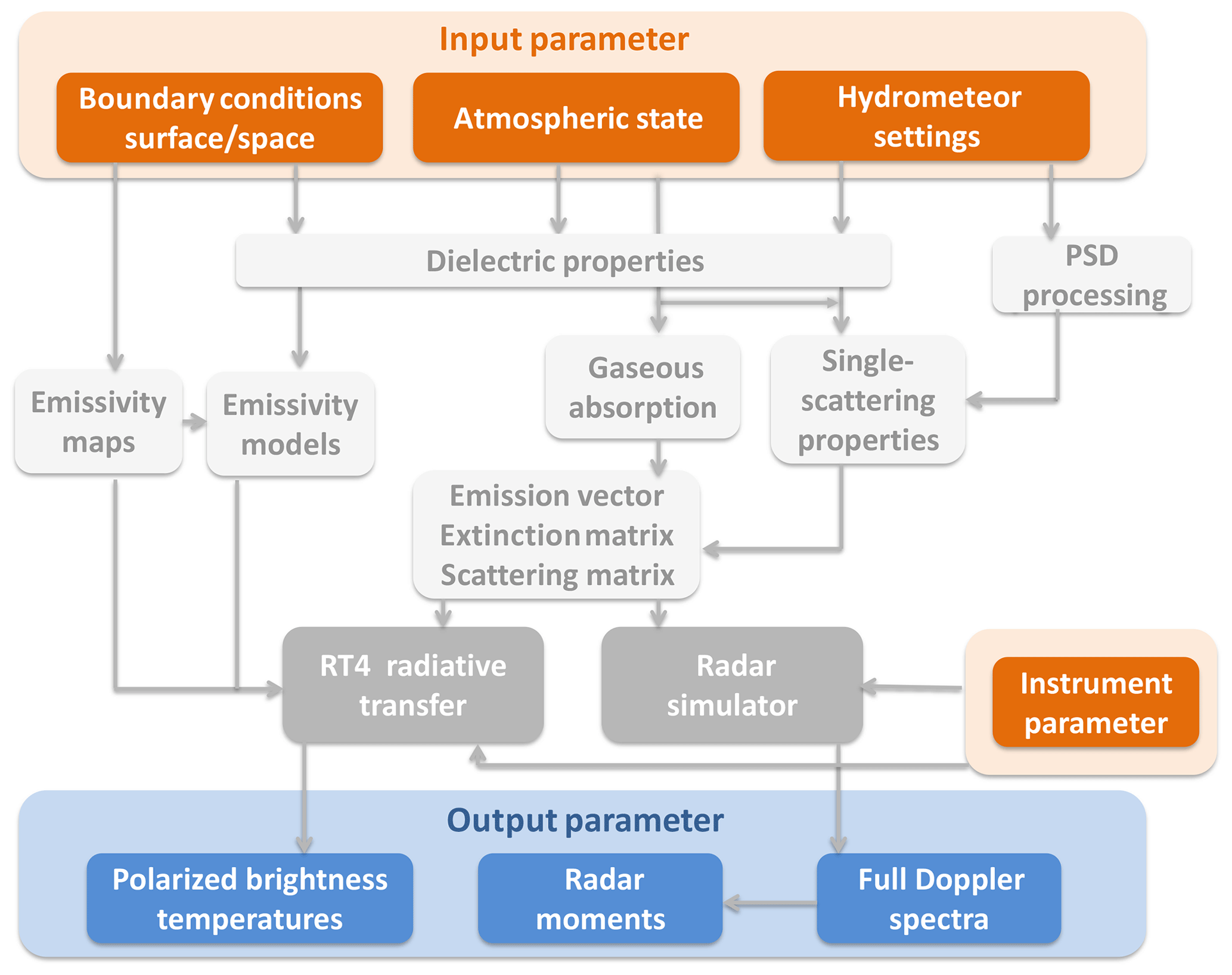
Figure 1Flowchart of the various steps performed during a PAMTRA simulation. Orange areas describe input parameters given by the user with the Python interface or text files. Gray boxes are the Fortran model parts where the various interaction parameters are generated and the radiative transfer or the radar simulator gets processed. Blue boxes describe the model output.
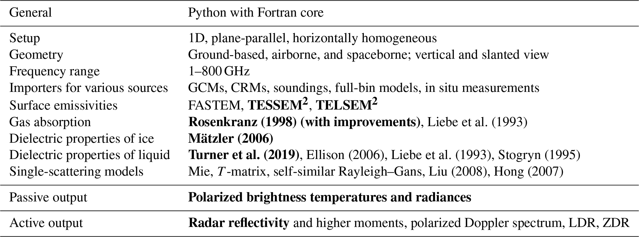
PAMTRA is a Fortran–Python model framework for the simulation of passive and active RT (including radar Doppler spectra) in a plane-parallel, one-dimensional, and horizontally homogeneous atmosphere for the microwave frequency range. Figure 1 shows a flow diagram of the various steps performed in the Fortran core of the present model setup. For the simulation, the model needs various inputs (shown in reddish colors) that describe the atmospheric state, the assumption on absorption, scattering, and surface emissivity, and instrument specifications. Depending on this input, the interaction parameters within various modules (white boxes) are generated. These parameters serve as input for the solving routines for the passive and active part (shown in gray). The simulations produce polarized radiances or brightness temperatures (TB) for the passive part and radar polarimetric Doppler spectra (and derived moments such as reflectivity, mean Doppler velocity, skewness, and kurtosis, as well as left and right slopes) for the active part. The simulation is performed at any observation geometry (zenith- and nadir-looking or slanted). Table 1 summarizes the main features of PAMTRA.
Rosenkranz (1998)Liebe et al. (1993)Turner et al. (2019)Ellison (2006)Liebe et al. (1993)Stogryn (1995)Liu (2008)Hong (2007)Table 1Main characteristics and features of PAMTRA. Default options are written in bold.
By pyPAMTRA a Python framework has been added around the Fortran core that allows calling PAMTRA directly from Python without using the Fortran I/O routines. Consequently, pyPAMTRA is a more user-friendly way to access the PAMTRA model and is the common way to use the model framework. It includes a collection of supporting routines, e.g., for importing model data or producing file or graphical output of the simulation results. With pyPAMTRA, parallel execution of PAMTRA on multicore processor machines and clusters is possible. Furthermore, by using Python for I/O and flow control, it is easier to interface PAMTRA to instruments or atmospheric models and post-processing routines.
2.1 Microwave radiometer simulator
For the passive part, the one-dimensional, polarized, and monochromatic vector RT equation for an azimuthally symmetric scattering media in a plane-parallel atmosphere applying the independent column approximation is solved using the RT4 code of Evans and Stephens (1995). 3D effects cannot be modeled, but horizontal inhomogeneity can be taken into account by the independent column approximation by realistically describing atmospheric variations along the path (Meunier et al., 2013). The assumption of a plane-parallel geometry is sufficient for most RT problems in the microwave spectral range with the exception of strongly scattering precipitation situations in which the radiation does not originate within the instruments' field of view (Battaglia and Tanelli, 2011). The RT equation is described by the formulation in Eq. (2.22) by Evans and Stephens (1993) or Eq. (1) in Evans and Stephens (1995). It is solved numerically by the doubling and adding method, which is formulated and described in detail by several textbooks (i.e., Liou, 2002, p. 290). RT4 requires as input the vertical profiles of temperature and gaseous absorption coefficients and a lower and upper boundary condition. If hydrometeors are present, the profiles of the single-scattering properties are required as well. Since a plane-parallel geometry with isotropic thermal emission is considered and all the particles are assumed to be azimuthally randomly oriented and mirror-symmetric, the radiation fluxes are also isotropic in azimuth. This symmetry in azimuth implies that the third and fourth Stokes components are zero and the RT problem simplifies to the first two components. RT4 does not make use of the Rayleigh–Jeans approximation, which relates the Planck function linearly to the brightness temperature and is widely used in the microwave regions.
As mentioned above, the doubling and adding are done in PAMTRA by RT4. In comparison to the formerly introduced RT3 (Evans and Stephens, 1991), RT4 enables the user to perform polarized RT calculations for particles that are nonspherical and holding a preferential horizontal alignment. Since one of the major goals in developing PAMTRA was to handle hydrometeor interactions as flexibly as possible, the possibility to simulate the RT for oriented particles with any shape is mandatory. RT4 calculates polarized TB (vertical and horizontal) for each discrete quadrature angle and frequency as well as upward- and downward-looking geometries at any height within the atmosphere.
2.2 Radar simulator
The PAMTRA radar simulator estimates the full radar Doppler spectrum based on the single-scattering properties of each hydrometeor species (see Sect. 2.5.2); it is mainly based on the concepts developed by Oue et al. (2020). First, the backscattering cross section σB(D) in square meters (m2) of the individual hydrometeor particles with maximum dimension D is converted to the volumetric backscattering ηD(D) in the unit of spectral radar reflectivity ():
where λ is the wavelength in meters, n(D) is the normalized PSD (m−4), and is the dielectric factor of water related to the refractive index. It is a common convention to use the value for liquid water at centimeter wavelengths (; Ulaby et al., 1981) regardless of whether ice or liquid clouds are observed. Nevertheless, as also depends on frequency, it is possible to change it for optimal adaptation to a specific problem. Currently, the simulation of multiple-scattering effects is not implemented in PAMTRA. Multiple scattering generally increases with the number of scatterers, with a larger measurement volume, and with increasing radar frequency (Battaglia et al., 2010). For satellite radars, such as CloudSat, multiple-scattering effects have to be accounted for in the case of heavy precipitation events (Matrosov and Battaglia, 2009). Due to the smaller measurement volume of common ground-based cloud radars, multiple scattering can usually be neglected for this application.
The radar reflectivity factor Ze can simply be obtained from Eq. (1) by integrating over the PSD. Unlike other radar simulators (e.g., Haynes et al., 2007; Buehler et al., 2005), PAMTRA provides the option to simulate the full radar Doppler spectrum, which is necessary to derive higher radar moments (mean Doppler velocity MDV, skewness, kurtosis). Deriving the radar moments from the simulated spectra also allows the user to account for instrument-specific characteristics such as the intensity and variance of the spectral noise. Those instrument characteristics can have an impact on the derived moments and are hence important to take into account when aiming to simulate observations of a specific radar system (see also examples in Sect. 3). The radar Doppler spectra simulator included in PAMTRA is partly based on the concept of Kollias et al. (2011, 2014), and the basic working principle is explained in the following.
As the measured Doppler spectrum is a function of fall velocity rather than particle size, the size descriptor of the spectral radar reflectivity ηD is changed from D to fall velocity v with
where, after the transformation by the differential (measured in s), the spectral radar reflectivity ηv(v) assumes the measuring units of . The user can choose between various hydrodynamical models to estimate hydrometeor terminal velocity v and based on their physical properties and environmental conditions such as air density, temperature, and pressure. For liquid drops, PAMTRA uses the relation provided by Khvorostyanov and Curry (2002) as a default. For ice and snow particles, the modified relation by Heymsfield and Westbrook (2010) is recommended because it is in better agreement with recent experiments using ice analogs (Westbrook and Sephton, 2017). For PAMTRA, v is defined such that positive values refer to particles moving towards the radar.
The velocity resolution of ηv(v) is related to the bin spacing of the particle size distribution. The maximum–minimum Doppler velocity of a real radar Doppler spectra is determined by the Nyquist velocity , which depends on the pulse repetition frequency PRF and the radar wavelength λ used. The velocity resolution is determined by the number of fast Fourier transform (FFT) points nfft used to derive the radar Doppler spectrum. These parameters are adjustable in the radar Doppler spectra simulator. The ηv(v) of all hydrometeors is then linearly interpolated onto the spectral resolution of the simulated radar. Furthermore, if the fall velocity exceeds vnyq, the simulator adds velocity-folding effects (aliasing) to the spectrum.
In reality, the idealized ηv(v) spectrum is affected by attenuation, kinematic broadening, vertical air motion, and radar noise (Doviak and Zrnic, 1993). In PAMTRA, the attenuated ηv(v) is obtained by subtracting the cumulative path-integrated attenuation, which is estimated from the extinction of gases and hydrometeors depending on measurement geometry (ground-based, airborne, or space-based). Kinematic broadening is assumed to have a Gaussian distribution that is convoluted with ηv(v) to simulate the broadening of the Doppler spectrum due to air motions (Gossard and Strauch, 1989) as described in detail in Maahn et al. (2015). In addition to kinematic broadening, a constant vertical air motion Vair can also be added that shifts the Doppler peak in the velocity spectrum without broadening the peak. To account for the radar receiver noise, the radar receiver noise power NP (unit: mm6 m−3, in accordance with Ze) is added to the spectrum ηv(v). To account for the loss of radar sensitivity due to range, NP is scaled with range squared. Because the noise is assumed to be white, random perturbations are added to every bin i of the spectrum in order to account for random noise effects following Zrnić (1975). To make the simulations by the radar simulator reproducible, the random seed used to obtain r(i) can be defined in PAMTRA. Finally, the spectrum is successively averaged nave times to account for smoothing and turbulence broadening.
Once the simulation of the nonidealized radar Doppler spectrum is complete, the corresponding moments are estimated similar to a real radar data processing scheme (e.g., Maahn and Kollias, 2012): first, the noise is removed from the spectrum; second, the moments of the hydrometeor peak are determined. In the case of several hydrometeor peaks in the same spectrum that are fully separated by the noise floor (multimodal spectra, e.g., Williams et al., 2018), PAMTRA can estimate the moments of individual peaks independently ordered by maximum spectral reflectivity. The main difference to a real radar data processing scheme is that the noise Ni is already known in advance. Therefore, the user can choose between using the known Ni or applying the method by Hildebrand et al. (2002) for estimating Ni. Based on the noise-corrected radar Doppler spectrum ηv(i)′, the moments (Ze, MDV, Doppler spectrum width σ, skewness γ, and kurtosis κ) and slopes (left, right) of the radar Doppler spectrum are estimated as discussed in Maahn and Löhnert (2017). The higher moments and the slopes depend on the instrument noise; therefore, it is crucial to configure PAMTRA in accordance with the radar specifications. All radar moments and the Doppler spectrum are available nonpolarized (NN), but if required also for HV (horizontal receive, vertical transmit), VH, VV, and HH polarization. This allows for the estimation of differential reflectivity and the linear depolarization ratio , among others.
2.3 Gaseous absorption
Absorption by atmospheric gases in the microwave range can be separated into contributions by resonant line absorption (i.e., H2O, O2, and O3) and the water vapor and dry continuum. PAMTRA implements various models to calculate the absorption coefficients of atmospheric gases. The model by Rosenkranz (2015), including modifications of the water vapor continuum absorption (Turner et al., 2009) and the line width modification of the 22.235 GHz H2O line (Liljegren et al., 2005), is selected as default. Alternatively, the Millimeter-wave Propagation Model (MPM93) developed by Liebe et al. (1993) can be used to simulate the absorption by the gaseous atmosphere. The clear interface structure of PAMTRA gives the possibility to easily include future improvements in gas absorption models, i.e., developments of models in the submillimeter wavelength range (Mattioli et al., 2019), and the implementation of absorption catalogs (Feist, 2004). This provides the possibility to also account for trace gases, which show abundant but weak absorption features in the microwave frequency range above 200 GHz.
2.4 Boundary conditions
The atmosphere is bounded at its upper end by the free space. The radiation emitted by this upper boundary can be described by the cosmic background with its mean radiative temperature of 2.73 K (Fixsen, 2009). The lower boundary of the atmosphere interacting with radiation is the Earth's surface. Thereby, the amount of radiation emitted in each upward direction is defined by the surface temperature and its type, which is determined by setting the emissivity and the model of scattering or reflection. This is not only important for upwelling geometries but also for downwelling in the case of a strongly scattering atmosphere (Kneifel et al., 2010). In PAMTRA, scattering and reflection properties of the surface are estimated assuming either a specular, Lambertian, or Fresnel reflection type (Mätzler, 2006, p. 225). Reflection on natural surfaces can be described by Fresnel equations. For idealized simulations, the emissivity can be fixed. Over land surfaces, PAMTRA makes use of the Tool to Estimate Land Surface Emissivity from Microwave to sub-Millimeter waves (TELSEM2; Wang et al., 2017; Aires et al., 2011), which provides emissivities based on geographic location and time information as angle- and frequency-dependent monthly mean values based on satellite observations.
The reflection of flat ocean surfaces can also be calculated with the Fresnel reflection formulae. The intensity of the reflection is strongly polarization- and angle-dependent and characterized by the dielectric properties of the ocean surface as a function of the sea surface temperature and salinity. With the Fresnel reflection formulae, the reflection coefficients and the Stokes reflection matrix can be calculated, as can the angle- and polarization-dependent emissivity. Since the reflection and emissivity calculated with the Fresnel relations are valid for calm surfaces and deviate significantly for high wind speeds, corrections for wind speed and therefore sea surface roughness and foam coverage have to be applied. PAMTRA utilizes the Tool to Estimate Sea‐Surface Emissivity from Microwaves to sub‐Millimeter waves (TESSEM2; Prigent et al., 2017). It is based on the FAST microwave Emissivity Model (FASTEM; Liu et al., 2011) and is designed for frequencies up to 700 GHz.
2.5 Hydrometeor description
PAMTRA has been designed to be flexible considering the treatment of hydrometeors, enabling the use of a wide variety of input data. Hydrometeor classes can be defined in a flexible way that allows for the exact matching of the properties of particles measured, e.g., by in situ microphysical probes or for consistency with assumptions on PSD, density, and shape made in CRMs. In addition to the assumptions on hydrometeors, the calculation of their interaction parameters (mainly absorption, scattering, and backscattering) and the integration over the PSD of the specific hydrometeor class are central parts of the RT framework (Johnson et al., 2012).
PAMTRA can handle a flexible number of hydrometeor classes. As an example, for the simulations based on the output of a CRM (see example Sect. 3.2), which provides hydrometeor content and total number concentration for cloud liquid, cloud ice, graupel, snow, rain, and hail, the number of hydrometeor classes would be six. For each hydrometeor class, the user can specify their microphysical and scattering properties.
The single particle properties are defined in PAMTRA with respect to the particle 3D maximum dimension (D), which is also uniquely defined for complex shapes such as snowflakes. Microphysical properties, such as PSD, mass–size relation, and velocity–size relation, can be easily defined by the user with the help of built-in functions. The user can select either size-resolved distributions of particles directly or the functional form of the PSD.
2.5.1 Particle size distribution
Most atmospheric models assume a moment-based bulk microphysical scheme for the treatment of cloud processes. In these schemes, the PSD for each hydrometeor category is assumed to follow a predefined functional form, and one or multiple moments of the PSD are simulated as prognostic variables. Using PAMTRA, it is straightforward to ingest the moments of the hydrometeor distributions and reconstruct the full PSD from them.
The PSD forms that are built into PAMTRA include the monodisperse, the inverse exponential, the modified gamma, and lognormal distributions. Some variations of these four main distributions have been implemented to facilitate the interface with some specific weather models. As an example, the formulation used by the two-category ice scheme in the COSMO model (see Doms et al., 2005, p. 69) assumes monodisperse distribution whereby the number concentration is dependent on the ambient temperature. Also, the relations reported by Field et al. (2005) and Ryan (2002) relating the inverse exponential distribution parameters to the atmospheric temperature and hydrometeor content are already implemented.
In the PSD construction, one or two PSD parameters are free parameters depending on the settings. PAMTRA derives the values of the unknown parameters by resolving the system of equations for the moments Mk that are given by the model output. The kth moment of a generic size distribution f(D) is defined as . At the current development stage, PAMTRA can use three different quantities related to the PSD moments as input, namely the total number concentration NT=M0, the effective radius , and the mass mixing ratio q=aMb, where a and b are the parameters of the power law defining the mass–size relation m(D)=aDb.
PAMTRA can also handle size-resolved distributions of particles, giving the largest flexibility in the definition of hydrometeor content and properties. With this tool, it is possible to set the properties (i.e., mass, area, hydrometeor terminal velocity) of particles for each size range, allowing PAMTRA to ingest in situ observations (see example Sect. 3.4) or the output of numerical models employing size-resolved (binned) microphysical schemes. This flexible interface can also be used to connect PAMTRA with atmospheric models that do not require predefined hydrometeor properties such as those involving the Particle Prediction Properties (P3; Morrison and Milbrandt, 2015) microphysical scheme or even the semi-Lagrangian super-particle models used for snow (McSnow; Brdar and Seifert, 2018) and drizzle formation (Hoffmann et al., 2017; Maahn et al., 2019).
2.5.2 Single-scattering and absorption properties
For liquid hydrometeors, such as cloud droplets, drizzle, or raindrops, the single-scattering properties are calculated using Mie theory (Mie, 1908). A large number of refractive index models for liquid water have been published over the last decades (Liebe et al., 1991, 1993; Ellison, 2006, 2007; Stogryn, 1995; Rosenkranz, 2015; Turner et al., 2016). Some of them, such as Liebe et al. (1991, 1993), are well accepted and very commonly used for liquid water in microwave RT. For liquid water at temperatures higher than 0 ∘C and the lower-frequency range (<150 GHz), the refractive indices of various models are relatively similar. However, for supercooled liquid water (i.e., liquid water at temperatures below freezing) and higher frequencies, the models increasingly deviate from each other because laboratory measurements of the refractive index in this region are lacking (Kneifel et al., 2014; Cadeddu and Turner, 2011). Recent observations of supercooled clouds at various sites (Kneifel et al., 2014) triggered the development of new refractive index models that combine the existing laboratory data set with the new cloud observations (Rosenkranz, 2015; Turner et al., 2016). The model of Turner et al. (2016) is used as the default liquid water refractive index model in PAMTRA. Other models, such as Liebe et al. (1993), Ray (1972), Stogryn (1995), and Ellison (2006), can be chosen by the user in order to allow comparison studies with other RT models or with previous RT simulations.
Frozen hydrometeors, such as ice crystals, snowflakes, or rimed particles, comprise a large natural variability of habits, densities, and orientations. This variability also affects their interaction with electromagnetic radiation, which explains the still large uncertainties in simulating their radiative properties. As a result, the number of scattering databases with various levels of complexity is rapidly increasing (Kneifel et al., 2018). In PAMTRA, there are several options regarding the definition of particle properties and the selection of scattering models. If the ice refractive index is not implicitly included in the selected scattering database, it is calculated using the model by Mätzler (2006).
Some of the most widely used approximations for ice and snow particles are spheres or spheroids (Bennartz and Petty, 2002; Petty, 2001; Honeyager et al., 2016; Hogan et al., 2012; Tyynela et al., 2011; Matrosov, 2015). Frozen hydrometeors are usually not composed of a homogeneous medium but rather a mixture of ice, air, and liquid water. Hence, spheroidal approximations always require the calculation of an effective refractive index. In PAMTRA, the generic mixing rule by Sihvola and Shivola (1989) is used. It should be noted that differences between various mixing formulas might be significant, and we have adopted the mixing rule that Petty and Huang (2009) found to cause the smallest deviation of the scattering properties of spheres when compared with more realistic snowflake shapes. PAMTRA allows defining either a constant density or a size-dependent mass–size relation. Dependent on the requirements on computational speed and particle properties, the scattering properties can be calculated using Mie (Mie, 1908) or T-matrix theory (Mishchenko and Travis, 1994); for the latter, the orientation and aspect ratio of the particles also have to be defined.
The spheroidal approximations, in particular the effective refractive index calculations, become increasingly unrealistic as soon as the wavelength becomes similar to the particle size. However, the size at which more complex particle models should be used also depends on the scattering variable (Schrom and Kumjian, 2017). The Discrete Dipole Approximation (DDA; Purcell and Pennypacker, 1973) is considered a reference method to compute the scattering properties of complex-shaped particles. An increasing number of databases with various particles and scattering variables have been developed during recent years (Kneifel et al., 2018). At the moment, the user can select particles of the DDA databases from Liu (2008) and Hong et al. (2009), which provide a number of single ice crystal types and a small number of aggregates. In particular for aggregates, PAMTRA also includes the very recent SSRGA for active and passive simulations (Hogan et al., 2017). The SSRGA is a cost-effective method to calculate the full phase function representative for an ensemble of aggregates. Unlike the soft spheroidal approximations, no effective refractive index is needed, but the fluctuations of mass, which mainly characterize non-Rayleigh scattering, are described with a number of coefficients. Those have been derived from a large ensemble of aggregates as described in detail in Hogan et al. (2017). The method is also applicable with reasonable accuracy to light and moderately rimed aggregates (Leinonen et al., 2018). A limitation of the SSRGA is that polarimetric variables cannot be estimated because the interaction of the scattering elements inside the particle is neglected. To our knowledge, PAMTRA is the first RT model that allows the use of SSRGA for passive microwave simulations.
When developing PAMTRA, specific emphasis was on its ability to interface a broad spectrum of microwave instruments and observing geometries with common atmospheric models and their different output variables and hydrometeor schemes. Here, we demonstrate the high versatility of PAMTRA with a number of application examples based on data from recent field campaigns and state-of-the-art atmospheric models.
All following simulations assume spheres (Mie) for the hydrometeor categories liquid water, rain, graupel, and hail. The SSRGA with the coefficients as in Mason et al. (2019) are used for cloud ice and snow. Herein, using the SSRGA allows us to ensure maximum consistency regarding particle properties such as the mass–size relation assumed in the microphysical schemes. The benefit of the SSRGA is illustrated for satellite measurements within a case study using the Integrated Forecasting System (IFS) from the European Centre for Medium-Range Weather Forecasts (ECMWF) model output together with passive microwave satellite observations (Sect. 3.1). How PAMTRA can be used for understanding cloud and precipitation processes as well as their representation in the novel ICOsahedral Non-hydrostatic atmosphere model (ICON; Zängl et al., 2015) is shown for both ground-based (Sect. 3.2) and airborne measurements (Sect. 3.3). While PAMTRA is interfaced with the two-moment microphysical scheme by Seifert and Beheng (2006) for the ICON application, Sect. 3.4 demonstrates PAMTRA's ability to ingest spectrally resolved information – in this case provided by airborne in situ measurements. The scripts to reproduce the simulations and all following figures are available in the Supplement.
3.1 Satellite perspective
Microwave satellite observations from polar orbiters, e.g., the Advanced Microwave Sounding Unit-A/B (AMSU-A/B) and the Microwave Humidity Sounder (MHS), have provided fundamental insights into tropical storms due to their unique ability to penetrate even opaque cloud systems (Kidder et al., 2000). Furthermore, their assimilation into NWP strongly contributes to forecast skills (Geer et al., 2017), though assimilation at higher frequencies becomes difficult due to the complex interaction of microwave radiation with frozen hydrometeors in the forward simulation.
To illustrate the benefit of the SSRGA compared to the conventional Mie approach for frozen hydrometeors, we selected a scene from ex-tropical storm Karl, which was investigated during the North Atlantic Waveguide and Downstream impact EXperiment (NAWDEX; Schäfler et al., 2018). The ECMWF IFS cycle 41r2 with a 0.1∘ grid (6 to 7 km) resolution provides the atmospheric input fields for PAMTRA. The IFS applies a one-moment microphysical scheme having four hydrometeor categories with the monodisperse cloud categories liquid and ice and exponentially distributed rain and snow (Forbes et al., 2011) as prognostic variables. Because the convective rain and snow flux profiles are not available in the standard output, we – in contrast to Geer and Baordo (2014) – cannot consider their contribution, which may modify the results. More details on the treatment of the IFS microphysics in PAMTRA are given in Appendix A1.
Microwave TB contains frequency-dependent contributions from atmospheric gases and hydrometeors that are difficult to disentangle as can be seen for AMSU-A/MHS measurements (Fig. 2a–c). Liquid clouds and precipitation usually appear as enhanced TB over radiatively cold surfaces like the ocean (emissivity of 0.5–0.7). Scattering at frozen hydrometeors, i.e., ice, snow, graupel, or hail, leads to a depression in TB (observed from space), which becomes stronger with increasing frequency. Due to the also increasing absorption by water vapor with higher frequencies, the surface influence is reduced and the scattering effects are better distinguishable from the surface effects (Skofronick-Jackson and Johnson, 2011). In order to illustrate the scattering effect, three window channels, i.e., 50.3, 89, and 157 GHz, were selected. The observed scenes clearly reveal the cyclonic nature of the storm. The occurrence of snow precipitation in its northeasterly sector can be clearly identified by its scattering effect, which leads to stronger decreases in TB with increasing frequency (Fig. 2a–c).

Figure 2Observations with AMSU-A at 50.3 GHz (a) as well as MHS at 89.0 (b) and 157.0 GHz (c) for ex-tropical cyclone Karl on 26 September 2016 during the NAWDEX campaign over the North Atlantic; simulations with IFS and PAMTRA with single-scattering properties calculated with Mie theory (d–f) and simulations with SSRGA for ice and snow (g–i). Difference in TB for Obs-Mie (j–l), Obs-SSRGA (m–o), and SSRGA-Mie (p–r). Integrated contents as the sum of cloud water and rainwater path (CWP+RWP) (s), ice water path (IWP) (t), and snow water path (SWP) (u).
PAMTRA was run twice, once using Mie theory for the calculation of the single-scattering properties of cloud ice and snow particles and once using the SSRGA. To match the output to the satellite observation, simulated TB values were convoluted according to the satellite geometry. Looking at the differences in TB between observation and both simulations (j–o), it can be seen that, especially for the lower two frequencies, the simulations show slightly lower values, especially in the southern part of the area. At these frequencies, the signal is mainly driven by emissions from the surface, water vapor, and liquid hydrometeors but not so much by scattering at frozen hydrometeors (Skofronick-Jackson and Johnson, 2011). Since the ocean surface signal in the microwave region can be model quite well by TESSEM2 and the sea surface temperature in the model and reality does not differ that much, the differences in TB can most likely be attributed to an underestimation of the liquid water contents (Fig. 2s) or the water vapor field (not shown). At the higher frequency of 157 GHz (Fig. 2l, o), the scattering at larger frozen hydrometeors becomes more important. In the Mie simulation, a clear underestimation of the scattering effect can be noted as no TB depression is present in the simulated field (Fig. 2f), although the IFS produces considerable amounts of snow as shown in the integrated hydrometeor contents with a snow water path up to 6 kg m−2 (Fig. 2u). The underestimation of the scattering by Mie theory is in accordance with previous studies that find spherical particles introducing significant positive biases in simulated TB (Geer and Baordo, 2014). In contrast, simulations with SSRGA (Hogan and Westbrook, 2014; Hogan et al., 2017) are in general able to produce TB depressions in agreement with the observations. For the simulations shown here based on IFS and PAMTRA using SSRGA for the frozen hydrometeors, the depression is much stronger than for Mie (Fig. 2r), and comparing it to the observation (Fig. 2o), it can be seen that it is even stronger than in the observation of MHS for the northeastern area, although the contributions to the total precipitating hydrometeor amount through convection are not included in the simulations. With the aforementioned capability of SSRGA to reproduce TB depressions in agreement with observations, this overestimation might be connected to either an overestimation of the snow water content of ECMWF IFS, especially in the middle and upper troposphere, or to an overestimation of the scattering by the SSRGA.
3.2 Ground-based perspective
Novel remote sensing instrumentation combined with high-resolution modeling is seen as a way forward to better understand cloud and precipitation processes. In this case study, we demonstrate how PAMTRA can be used to simulate a wealth of state-of-the-art ground-based active and passive microwave observations including radar Doppler spectra at multiple frequencies. The observations shown in Fig. 3 were recorded on 19 November 2015 as part of the TRIple-frequency and Polarimetric radar Experiment for improving process observation of winter precipitation campaign (TRIPEx; Dias Neto et al., 2019) at the Jülich Observatory for Cloud Evolution Core Facility (JOYCE-CF; Löhnert et al., 2015). The data have been carefully quality-controlled and corrected for radar calibration biases and attenuation by gases and hydrometeors as described in detail in Dias Neto et al. (2019).
The novel ICON model in its large eddy version (ICON-LEM; Heinze et al., 2017), with a horizontal resolution of 600 m and 150 vertical layers, is used as input to PAMTRA. ICON-LEM is forced by initial and lateral boundary conditions from the ECMWF IFS. The ICON-LEM version used here implements the two-moment microphysical scheme from Seifert and Beheng (2006). The cloud scheme has six hydrometeor classes (cloud drops, rain, cloud ice, snow, graupel, and hail), which are assumed to be distributed according to a modified gamma function (Petty and Huang, 2011). The model simulates the evolution of two moments of the hydrometeor distributions, namely the mass mixing ratio q and the total number concentration N. Details on the treatment of the ICON microphysical scheme are given in Appendix A2. The forward simulations take the different radar specifications (e.g., sensitivity, beam widths, and averaging interval) as described in Dias Neto et al. (2019) into account. TB is simulated for the 14 channels of the Humidity and Temperature PROfiler (HATPRO; Rose et al., 2005). The passage of a cold front on 19 November 2015 (Fig. 3) is nicely captured by the ICON simulations regarding both vertical and temporal evolution. The first 6 h of model simulations are likely affected by the spin-up of the model (started at 00:00 UTC) and have therefore been excluded from the figure.
The cloud and precipitation field associated with the cold front causes similar reflectivity structures in the forward simulations as observed. Although the ICON–PAMTRA setup currently does not include a melting layer model, the transition from ice to rain at 1.5–2 km can be clearly seen in the reflectivity and particularly in the mean Doppler velocity (note the well-matched increase in melting layer height). During periods of most intense rainfall (up to 5.6 mm h−1 between 14:00 and 15:00 UTC), attenuation effects are somewhat overestimated in the model, but overall the observed signatures are well captured. Passive observations are unreliable during rainy periods due to potential liquid water on the radome (Cadeddu et al., 2017). During non-precipitating conditions, the overall spectral response of the different channels matches the observations very well, although the high-frequency fluctuations associated with liquid cloud in the observed TB are missed. This might be due to the lower spatiotemporal resolution of the ICON simulation that reproduces the basic temporal evolution, but small-scale fluctuations cannot be captured with the resolution used.
A more detailed comparison of modeled and observed microphysical processes is possible due to the ability of PAMTRA to simulate the entire radar Doppler spectrum (Fig. 4). The vertical distribution of the Doppler spectrum during the core precipitation period nicely shows the transition from the slow and narrow ice and snow spectra to wider and faster rainfall at around 2 km of height in both simulations and observations. In the ice part, the simulated spectra sometimes reveal bimodalities and fall velocities that are too large (up to 2 m s−1). This might indicate some discrepancies in the transition from ice to the snow hydrometeor category in the ICON model or rimed particles in the model with larger fall velocities that are not observed. The observations show at certain heights dynamical effects such as shifting due to vertical air motions or broadening due to turbulence. PAMTRA is in principle able to account for these effects if vertical air motion or the eddy dissipation rate is provided. Looking at individual spectra in the ice part (Fig. 4c, d), one can see that the noise levels and the shape and velocity region of the ice Doppler spectra are very well matched. In the rain part (Fig. 4e, f), the Doppler spectra reveal typical resonances at larger drop diameters (first minimum at 6 m s−1 corresponding to 1.7 mm size drops; Kollias et al., 2002), which are also well captured by the PAMTRA forward simulations. The differences in the noise levels (especially the Ka band) are due to known saturation effects in the Ka-band receiver that enhances the spectral noise. The slight mismatch of the W-band noise level is due to the height-dependent chirp table configuration and associated variable sensitivity (Küchler et al., 2018). In this simulation, PAMTRA was configured to match the highest chirp sequence, and hence the noise level at lower ranges is underestimated.
The ability of PAMTRA to consistently simulate a multitude of radar observables in combination with passive observations provides new opportunities to evaluate microphysics schemes on a process level. For example, the multifrequency radar observations can be used to distinguish aggregation- and riming-dominated regions (Kneifel et al., 2015). Additional constraints on, e.g., the assumed PSD or terminal velocity–size relation used in a microphysics scheme can be provided by multifrequency Doppler spectra (Li and Moisseev, 2019; Kneifel et al., 2016). Finally, the passive observations add information on temperature and humidity profiles as well as on vertically integrated liquid water and ice content (Kneifel et al., 2010). PAMTRA is thus not only an important tool to derive new retrievals (Maahn and Löhnert, 2017) but can also be used to develop new microphysical parameterizations as new schemes can be directly confronted with observational characteristics (e.g., typical properties of the radar Doppler spectra).
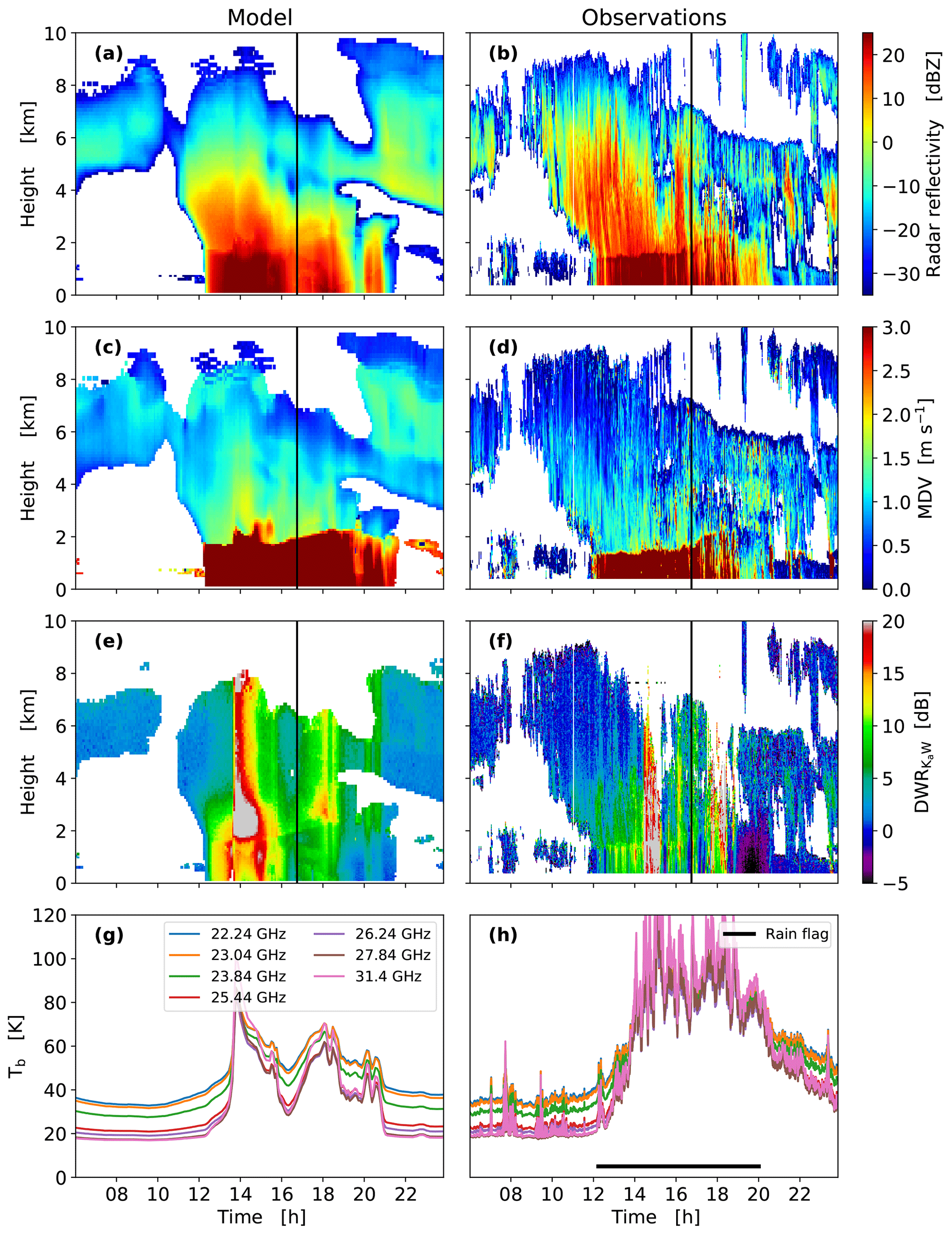
Figure 3Case study of a cold front observed at the JOYCE site on 19 November 2015. From top to bottom: time versus height above ground, showing equivalent radar reflectivity factor Ze (dBZ) at the Ka band (a, b), mean Doppler velocity MDV (m s−1) (c, d), dual-wavelength ratio DWR between the Ka and W band (dB) (e, f), and TB (K) of the HATPRO microwave radiometer for the seven water vapor channels (g, h). The right side shows the observations; PAMTRA simulations based on the ICON-LEM output are shown in the left column. The black horizontal bar in the HATPRO observation plots indicates periods of an active rain flag for the microwave radiometer; data during this period are likely to be disturbed by rain on the radome. The vertical black line in the radar time–height plots indicates the time used for the spectra comparison in Fig. 4.

Figure 4Comparison of simulated (a, c, e) and observed (b, d, f) Doppler spectra at 16:20 UTC for the same frontal case from 19 November 2015 shown in Fig. 3. From top to bottom: Ka-band spectrograms (a, b); example Ka- and W-band Doppler spectra in the ice (c, d) and the rain (e, f) parts of the cloud. The horizontal red lines in the spectrograms indicate the heights at which the example spectra of the successive panels have been extracted.
3.3 Airborne remote sensing perspective
Widespread Arctic mixed-phase clouds present one of the largest challenges to atmospheric models for weather and climate applications (Morrison and Milbrandt, 2015). Airborne campaigns can provide unique information in this area where ground-based observations are made at very few stations and where polar-orbiting satellites have a rather coarse spatial resolution. Here we want to demonstrate how airborne active and passive microwave observations can be exploited with the help of PAMTRA simulations to constrain microphysical schemes in CRMs. For this purpose, PAMTRA settings are adapted to mimic the measurements of upward-directed passive and active radiation made by the airborne Microwave Radar/radiometer for Arctic Clouds (MiRAC; Mech et al., 2019a) flown during the Arctic CLoud Observations Using airborne measurements during polar Day (ACLOUD; Wendisch et al., 2019) campaign. MiRAC combines a 94 GHz frequency-modulated continuous wave (FMCW) radar with its integrated passive 89 GHz channel and novel 180–340 GHz radiometer. It was operated aboard the Polar 5 research aircraft of the Alfred Wegener Institute, Helmholtz Centre for Polar and Marine Research (AWI), over the Arctic Ocean and the sea ice northwest of Svalbard in May–June 2017.
The measurements were taken on a flight section of research flight 5 in a cold air outbreak over the Fram Strait west of Svalbard on 25 May 2017 between 11:30 and 12:00 UTC. The aircraft was flying from west to east over open ocean perpendicular to the atmospheric flow. The reflectivity measurements shown in Fig. 5 nicely depict the typical roll cloud structure that develops when an Arctic air mass transitions from the central Arctic to the open ocean during a cold air outbreak (Liu et al., 2006). Their vertical extent is around 750 m with horizontal length scales of up to 3 km in the observations. By the strong reflectivities in the lowest atmospheric layers, it can be seen that some of the rolls are connected to precipitation, most likely as snow. The enhanced TB of the 89 GHz passive channel indicates the presence of liquid water over the radiatively cold ocean. A simple regression algorithm for liquid water path (LWP) has been derived from PAMTRA-simulated TB using nearby dropsondes and artificial clouds, giving an estimate of a maximum LWP of 80 g m−2.
Similar to the example shown for ground-based perspectives (Sect. 3.2), ICON-LEM was used to simulate the atmospheric conditions this time in a nested approach with the final horizontal resolution of 150 m. Two different simulations have been performed: the first with a standard, fixed vertical profile for cloud condensation nuclei (CCN) and ice nuclei (IN) and the second with a parameterization for CCN and IN activation based on Hande et al. (2016). For the second realization, the fixed profile was replaced by prognostic CCN and IN, and the major part of the change was caused by the activation scheme by Phillips et al. (2008). The sea surface emissivity is calculated by TESSEM2 based on the ICON-LEM input, i.e., wind speed and sea surface temperature. Gaseous absorption has been calculated according to the Rosenkranz 98 model.
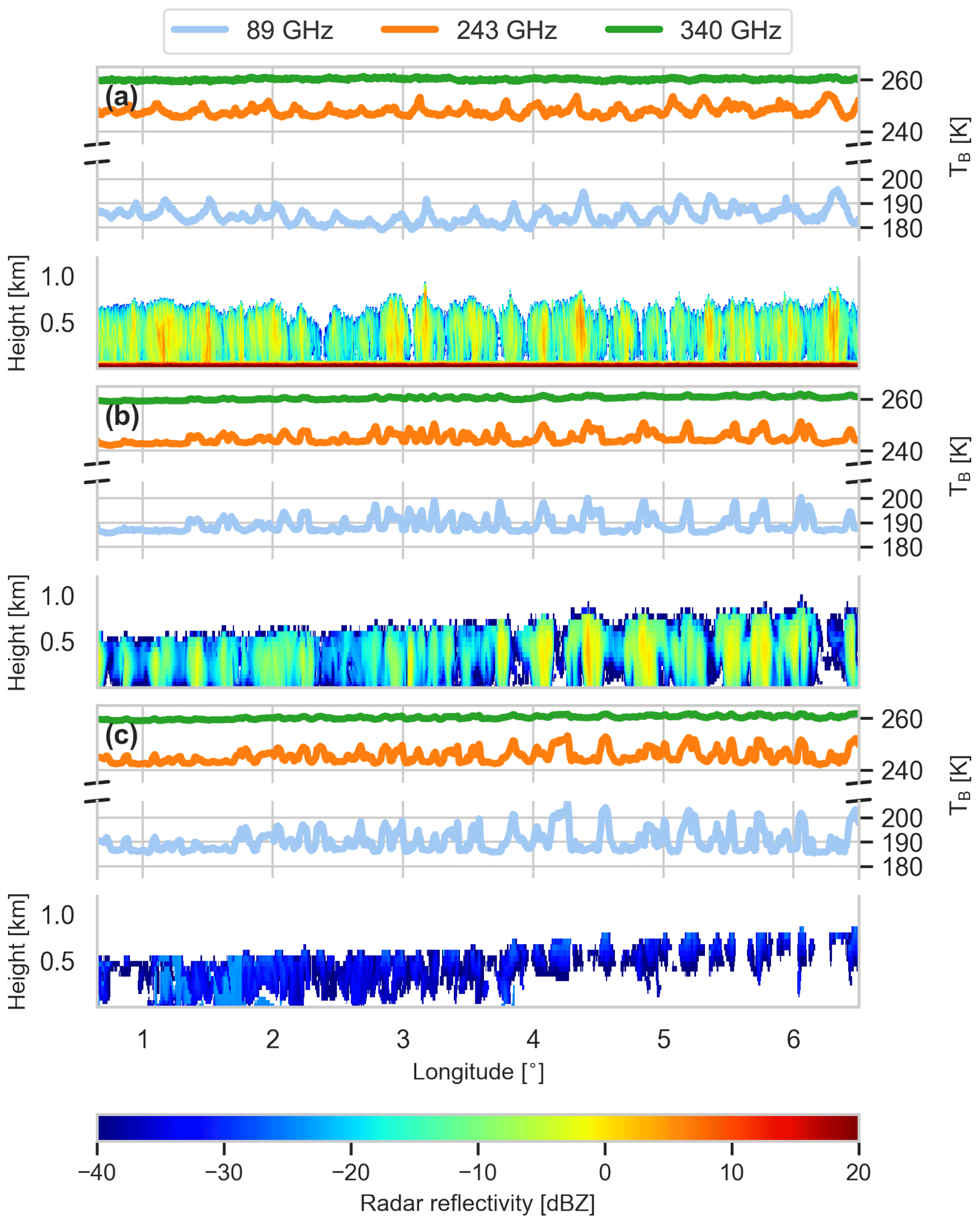
Figure 5Radar reflectivity at 94 GHz and TB at 89 GHz (blue) with horizontal polarization as well as at 243 (orange) and 340 GHz (green) with mixed polarization as measured by the MiRAC instrument (a) during a 30 min flight section in the west–east direction over the Fram Strait on 25 May 2017. Simulated radar reflectivity and TB with ICON-LEM and PAMTRA after improvements made to the microphysical scheme in ICON-LEM (b) and before (c). Note that the radar and 89 GHz measurements were performed under an angle of 25∘ backwards.
As can be seen in Fig. 5, the general structure of the roll clouds with an approximately 800 m top height is well captured with the ICON model resolution of 150 m in both simulations. The vertical and horizontal scales of the roll clouds are similar to the observations. The simulated radar reflectivities with the ICON standard setup (Fig. 5c) are much lower than the observed ones and basically confined to a cloud layer a few hundred meters thick. Hardly any precipitation reaching the ground is visible, in strong contrast to observations. Since the reflectivity at this frequency is mainly driven by large frozen hydrometeors, this indicates too few snow hydrometeors in the simulations. The simulated brightness temperatures agree better with their observational counterpart, though a slightly enlarged amplitude – indicating higher LWP – can be seen in the simulations. Looking at the ICON simulation with modified CCN and IN activation, radar reflectivities are generally enhanced compared to the original simulation, with maxima of +10 dBZ compared to −20 dBZ in the original run, and are now much closer to the observations. As the amplitude of the TB signal is slightly reduced, one can conclude that the modified scheme is able to convert liquid water more efficiently into ice precipitation.
For the same scene coarser-resolution ICON standard runs were also evaluated, which revealed an even larger underestimation of radar reflectivities. While much larger samples of observations and simulations are needed to draw solid conclusions, this case study demonstrates the ability of PAMTRA in testing different microphysical schemes and suitability.
3.4 Airborne in situ perspective
In the previous examples, typical bulk microphysical schemes were employed in atmospheric models that implicitly assume a functional relation of hydrometeor properties (e.g., PSD) to which the prognostic model variables, e.g., mixing ratios and number concentrations, can be directly related. New model developments, such as the P3 microphysical scheme (Morrison and Milbrandt, 2015), pose a challenge for RT as their hydrometeor properties, e.g., density, are variable. Similarly, Lagrangian super-particle models (Brdar and Seifert, 2018), models with full-bin microphysics, and box models (Hoffmann et al., 2017) require similar flexibility in the assumptions of hydrometeor properties from the RT. PAMTRA addresses those needs with a full-bin interface (Maahn et al., 2019). In order to demonstrate this feature, we simulate radar Doppler spectra based on airborne in situ observations of liquid clouds. The direct use, i.e., without the need to fit any functional form to the particle properties, of in situ observations in the RT provides numerous possibilities for closure studies between in situ and remotely sensed observations.
The in situ observations of liquid cloud properties have been obtained from the 5th Department of Energy Atmospheric Radiation Measurement (DOE ARM) Program's Airborne Carbon Measurements (ACME-V) campaign obtained at the North Slope of Alaska in summer 2015. The ARM Gulfstream G-159 (G-1) aircraft of the ARM aerial facility (Schmid et al., 2014, 2016) measured the cloud droplet number concentration for droplets larger than 1.5 µm using a combination of optical cloud probes. The probes and the processing of the cloud probe data set following Wu and McFarquhar (2016) are detailed in Maahn et al. (2017). In contrast to the other examples, no particle size distribution is assumed, but the measured PSD is directly used in PAMTRA through the full-bin interface. Besides the PSD, the particle mass, density, cross section area, and aspect ratio also need to be defined in PAMTRA for every size bin, which is trivial for liquid particles. To focus on the idealized development of the spectrum, vertical air motions are not considered in this example.
Figure 6 shows the observed PSD and the resulting simulated radar Doppler spectrum for a vertically sampled cloud at around 22:36 UTC on 27 June 2015. The observed PSD and effective diameter (the ratio of the third- and the second-moment analog to the effective radius) clearly show the increase in droplet size with increasing height caused by condensation. When forward-modeled with PAMTRA, this leads to an increase in Ze because droplet backscattering scales with diameter D6. In the height-resolved Doppler spectra (Fig. 6b), this is mainly reflected in the increased spectral reflectivity within the cloud mode with height. Herein, due to the low fall velocity of cloud droplets, their Doppler velocities are basically limited to below 0.5 m s−1, even close to cloud top where droplets are largest. However, the radar Doppler spectra reveal Doppler velocities up to 1 m s−1 at certain heights, sometimes showing a clear bimodality of the spectra, e.g., 800 and 1000 m. These can clearly be attributed to the high impact of low-concentration drizzle droplets on radar observations. These drizzle droplets are not visible in Fig. 6a despite the logarithmic color scale as they are rare. The small sampling volume of the optical probes used during ACME-V leads to poor statistics for drizzle drops, which can explain the presence of inhomogeneities in the spectra forward-modeled with PAMTRA (Fig. 6b). This example has shown how spectrally resolved information can be exploited by PAMTRA to investigate the impact of different hydrometeors on radar Doppler spectra. Even the simple example of liquid-only hydrometeors has shown the high impact of few larger particles on the shape of Doppler spectra. Therefore, higher moments of the Doppler spectra, e.g., skewness and kurtosis, contain information that can be used in retrieval algorithms to disentangle the cloud and drizzle contribution to Ze (Küchler et al., 2018). Fingerprinting of characteristic hydrometeor signatures in the spectra becomes even more important for frozen hydrometeors, allowing for detailed process studies (Kalesse et al., 2016).
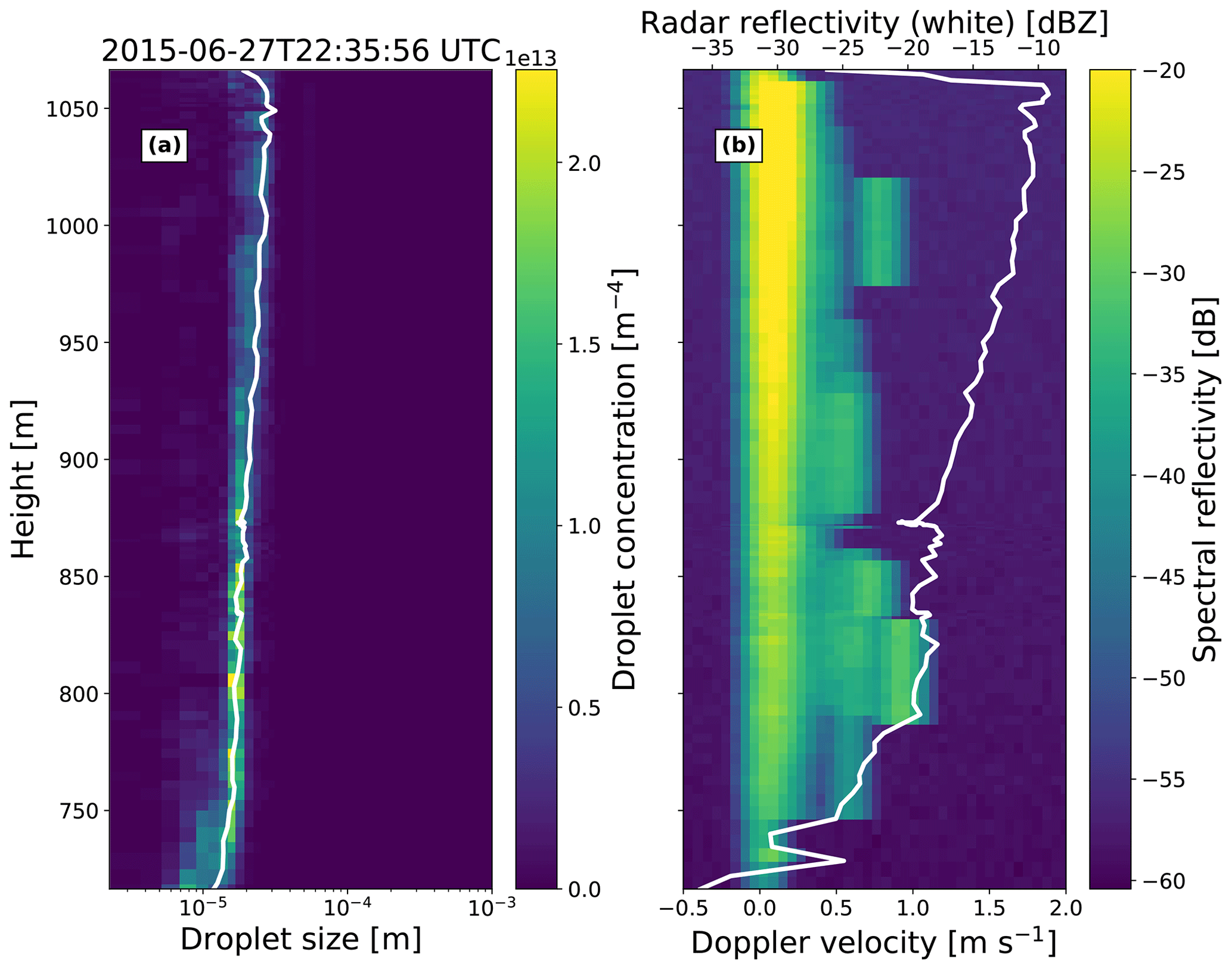
Figure 6(a) Observed drop size distribution and (b) forward-modeled radar Doppler spectrum of the sample cloud in the ACME-V campaign. The white line denotes (a) the effective diameter and (b) the radar reflectivity Ze.
This study introduced the first publicly available version of the PAMTRA forward operator, whose development was motivated by the growing interest in better exploiting the unique characteristics of microwave observations to provide information on clouds and precipitation. Specifically, the combination of passive and active microwave sensors on different platforms is very attractive due to their complementary information. To fully exploit the information of the measurements for process studies, as well as the evaluation and further development of cloud-resolving models, PAMTRA has been designed as a versatile tool to be compliant with a wide variety of model output and in situ observations as input. Furthermore, PAMTRA aims to support the ongoing development and application of ground-based instrumentation, in particular for multifrequency radar Doppler spectra measurements, airborne active–passive instrument packages, and satellite measurements, which will be further extended into the submillimeter range, i.e., by the Ice Cloud Imager (ICI; Kangas et al., 2014) including channels up to 664 GHz.
PAMTRA simulates one-dimensional radiative transfer in a plane-parallel atmosphere for the polarized passive and the full radar Doppler spectrum for active applications in up- and down-looking mode. PAMTRA has many features already included, i.e., different gas absorption modules, models for the calculation of the surface emissivity, and different methods to calculate the single-scattering properties of hydrometeors. Herein, it is unique as the SSRGA can be applied for both passive and active applications. Due to its modularity, it can be easily extended when new developments, e.g., new absorption models and single-scattering databases, become available. As some applications require massive calculations, e.g., databases for retrieval development or model evaluation, the implementation of parallelization features into PAMTRA supports high-performance computing.
Within an example section several applications of PAMTRA as a forward simulator were introduced, which can be reproduced by the interested reader with the help of Jupyter notebooks (https://github.com/igmk/pamtra/, last access: 6 September 2020). The examples consider different geometries, i.e., ground-based, aircraft, and satellite, and different input sources such as airborne in situ hydrometeor spectra, two-moment cloud-resolving model simulations, and NWP (ECMWF-IFS) analysis. It should be noted that the modular setup of PAMTRA also allows for simpler information such as idealized atmospheric profiles or radiosonde measurements. The latter are especially common for classical retrieval or information content studies for passive microwave measurements such as in Ebell et al. (2013).
The representation of cloud and precipitation processes is a long-standing problem for atmospheric models, and the development of new parameterizations and schemes is ongoing, in particular for frozen hydrometeors. Microwave scattering by frozen particles provides, on the one hand, insights into the dominating hydrometeors, and on the other hand it is also rather challenging due to the wide variety of particles and thus single-scattering properties. Progress can only be achieved by the interplay of cloud and RT modeling and its confrontation with measurements. In this context, the first example (Sect. 3.1) demonstrates that, especially for higher frequencies, i.e., millimeter and submillimeter range, the conventional Mie approach is not useful. PAMTRA can also use the T-matrix approach for single-scattering calculations, which, however, requires knowledge of particle orientation. Therefore, the SSRGA approach already used successfully in the radar community has also been implemented for passive RT and shows promising capabilities.
That the forward approach is helpful in disentangling the different contributions of hydrometeors in the measurements is illustrated by further examples. Herein it is important that PAMTRA can be run in high consistency with the models' microphysical assumptions. From the ground where novel technologies can be deployed fast, multiple-frequency radar provides exciting insights into precipitation formation via the ice phase (Sect. 3.2). Airborne measurements allow access to remote areas such as the Arctic where complex mixed-phase clouds are observed in cold air outbreaks. How active–passive microwave measurements of such clouds can constrain microphysical schemes in the novel ICON model is shown in Sect. 3.3 by the different response of radar reflectivities and brightness temperatures with respect to the relative contributions by frozen and liquid hydrometeors.
We did not show an example for the classical observation-to-model approach whereby databases of synthetic measurements and corresponding variables of interest are generated for subsequent retrieval development (e.g., Chaboureau et al., 2008). However, by illustrating how cloud droplet spectra from in situ measurements can be used as PAMTRA input for simulating radar Doppler spectra (Sect. 3.4) we could illustrate that higher moments of the spectra can be suitable as retrieval input as they show clear drizzle signatures (Acquistapace et al., 2019; Küchler et al., 2018). Along this line the passive microwave signatures of drizzle can also be simulated to support related retrieval development (Cadeddu et al., 2020). In general, PAMTRA is well suited for synergetic retrieval development as a multitude of microwave measurement quantities, i.e., multifrequency polarized brightness temperatures and Doppler spectra moments, can be simulated consistently for the same atmospheric scene.
For the future development of PAMTRA, namely PAMTRA2.0, it is planned to move on to an even more modular code based on Python3 to allow an enhanced parallelization. Further features to be taken into account in the development of PAMTRA2.0 are improvements in the simulation of spectral radar polarimetry, the parameterization of frozen surface emissivity, and simpler adaptations to slant observation geometry. Interested scientists are cordially invited to contribute to PAMTRA through our online repository.
This section provides details on how the model output of IFS and ICON-LEM is converted into hydrometeor PSDs in PAMTRA for the computations shown in the example in Sect. 3.1, 3.2, and 3.3.
A1 IFS microphysical scheme
The IFS model uses a one-moment microphysical scheme with four hydrometeor classes, namely cloud drops, cloud ice, snow, and rain. The prognostic moment simulated by the scheme is the mass mixing ratio q.
The liquid cloud drops and cloud ice are assumed to be monodispersed with all the particles having an equal maximum diameter D and an equal mass m. As a consequence of that these particles will also have an equal density ρ (Forbes et al., 2011), and therefore it is possible to derive the number concentration of the particles N by dividing q by the specific volume of the hydrometeors:
The rain and snow are assumed to be distributed according to an inverse exponential size distribution:
The relations between the mass and size of each particle and the N0 and Λ parameters of N(D) are both assumed to follow the power-law form
and
Equation (A5) is solved for Λ through the analytic inversion of the equation for the mixing ratio:
A2 ICON-LEM microphysical scheme SB06
As already mentioned in Sect. 3.2 and 3.3, the ICON-LEM version used in the examples implements the two-moment Seifert and Beheng (2006) microphysical scheme (hereafter SB06). SB06 predicts the evolution of six hydrometeor classes, namely cloud drops, rain, cloud ice, snow, graupel, and hail. For each of these hydrometeor classes it is assumed that the mass m is distributed according to a modified gamma distribution. Also, the mass of each hydrometeor is related to its maximum size through a power-law function:
and
By applying the change of variable rule f(m)dm=N(D)dD, one can see that the size distribution N(D) assumed in PAMTRA is again of the modified gamma functional form
The parameters of the PAMTRA size distribution N(D) (primed variables) can be derived from those of the mass distribution f(x) using the following substitutions:
with
and
For each hydrometeor class the parameters μ and γ are fixed and thus also the PAMTRA parameters μ′ and γ′. PAMTRA derives the free parameters and Λ′ by solving the system of equations for the two prognostic moments in the SB06 scheme:
and
which have an analytic solution through the use of the complete gamma function Γ(x) for values of .
The current version of PAMTRA can be found in a publicly available GitHub repository distributed under a GPLv3.0 license at https://github.com/igmk/pamtra (Mech et al., 2019c). The exact version of PAMTRA used for this paper is archived on Zenodo (https://doi.org/10.5281/zenodo.3582992, Mech et al., 2019b), including the scripts and data to produce the plots shown in the “Application examples” section. The code documentation and user manual are compiled into a “Read the Docs” web page available at https://pamtra.readthedocs.io (last access: 6 September 2020), and Jupyter notebooks that introduce the PAMTRA usage by presenting documented examples and links to the required data are included in the public GitHub repository.
MarM originally created the PAMTRA model framework consisting of the passive part and the basic methods for gaseous absorption and single-scattering calculations. MaxM developed the active radar simulator and the pyPamtra framework as well as designing the documentation and example framework. MarM and MaxM are the main authors of PAMTRA. PK supported the implementation of the radar Doppler spectra simulator in PAMTRA. DO implemented the SSRGA and is strongly involved in the complete development of the single-scattering section and the examples. SK significantly contributed to the methods of the model for the single-scattering calculations, the dielectric properties, and the gaseous absorption. EO designed the hydrometeor interface and the particle size distribution methods. VS performed the cloud-resolving model simulations with the ICON-LEM and is strongly involved in the interfacing of atmospheric models to PAMTRA. SC contributed to the interpretation of the simulation results and the basic model and paper design. MarM prepared the paper with contributions from all co-authors.
The authors declare that they have no conflict of interest.
The authors would like to thank K. Franklin Evans and Graeme L. Stephens for making their model RT4 publicly available.
The authors would also like to thank Heini Wernli for preparing the ECMWF data and Richard Forbes for his support in working with the ECMWF data.
We gratefully acknowledge the funding by the Deutsche Forschungsgemeinschaft (DFG, German Research Foundation) – Projektnummer 268020496 – TRR 172, within the Transregional Collaborative Research Center “ArctiC Amplification: Climate Relevant Atmospheric and SurfaCe Processes, and Feedback Mechanisms (AC)3”. Partial support for this research was provided by the DFG priority program “High Altitude and Long Range Research Aircraft (HALO)” SPP 1294 “Using the HALO Microwave Package (HAMP) for cloud and precipitation research”, grant CR 111/9-1.
This work was also partially funded by the Federal Ministry of Education and Research (BMBF) within the program High Definition Clouds and Precipitation for advancing Climate Prediction (HD(CP)2) under grant 01LK1211.
Contributions by Stefan Kneifel and Davide Ori were funded by the German Research Foundation (Deutsche Forschungsgemeinschaft, DFG) under grant KN 1112/2-1 as part of the Emmy-Noether Group OPTIMIce.
Maximilian Maahn was supported by the US Department of Energy (DOE) Atmospheric Systems Research (ASR) program (DE-SC0013306) and the National Oceanic and Atmospheric Administration (NOAA) Physical Sciences Lab (PSL). ACME-V data were obtained from the Atmospheric Radiation Measurement (ARM) Program sponsored by the US Department of Energy, Office of Science, Office of Biological and Environmental Research, Climate and Environmental Sciences Division. The authors would like to thank Greg McFarquhar and Wei Wu for supporting us with the use of ACME-V data.
This research has been supported by the Deutsche Forschungsgemeinschaft (grant nos. 268020496, CR 111/9-1, and KN 1112/2-1). The Federal Ministry of Education and Research (BMBF) supported this work with grant no. 01LK1211. The US Department of Energy (DOE) Atmospheric Systems Research (ASR) program supported the work with grant no. DESC0013306.
This paper was edited by Volker Grewe and reviewed by two anonymous referees.
Acquistapace, C., Kneifel, S., Löhnert, U., Kollias, P., Maahn, M., and Bauer-Pfundstein, M.: Optimizing observations of drizzle onset with millimeter-wavelength radars, Atmos. Meas. Tech., 10, 1783–1802, https://doi.org/10.5194/amt-10-1783-2017, 2017. a
Acquistapace, C., Löhnert, U., Maahn, M., and Kollias, P.: A New Criterion to Improve Operational Drizzle Detection with Ground-Based Remote Sensing, J. Atmos. Ocean. Tech., 36, 781–801, https://doi.org/10.1175/jtech-d-18-0158.1, 2019. a
Aires, F., Prigent, C., Bernardo, F., Jiménez, C., Saunders, R., and Brunel, P.: A Tool to Estimate Land-Surface Emissivities at Microwave Frequencies (TELSEM) for Use in Numerical Weather Prediction, Q. J. Roy. Meteor. Soc., 137, 690–699, https://doi.org/10.1002/qj.803, 2011. a
Battaglia, A. and Tanelli, S.: DOMUS: DOppler MUltiple-Scattering Simulator, IEEE T. Geosci. Remote S., 49, 442–450, https://doi.org/10.1109/TGRS.2010.2052818, 2011. a
Battaglia, A., Tanelli, S., Kobayashi, S., Zrnic, D., Hogan, R. J., and Simmer, C.: Multiple-Scattering in Radar Systems: A Review, J. Quant. Spectrosc. Ra., 111, 917–947, https://doi.org/10.1016/j.jqsrt.2009.11.024, 2010. a
Bennartz, R. and Petty, G. W.: The Sensitivity of Microwave Remote Sensing Observations of Precipitation to Ice Particle Size Distributions, J. Appl. Meteorol., 40, 345–364, https://doi.org/10.1175/1520-0450(2001)040<0345:tsomrs>2.0.co;2, 2002. a
Bodas-Salcedo, A., Webb, M. J., Bony, S., Chepfer, H., Dufresne, J.-L. L., Klein, S. A., Zhang, Y., Marchand, R., Haynes, J. M., Pincus, R., and John, V. O.: COSP: Satellite Simulation Software for Model Assessment, B. Am. Meteorol. Soc., 92, 1023–1043, https://doi.org/10.1175/2011BAMS2856.1, 2011. a
Borque, P., Luke, E., and Kollias, P.: On the Unified Estimation of Turbulence Eddy Dissipation Rate Using Doppler Cloud Radars and Lidars, J. Geophys. Res., 121, 5972–5989, https://doi.org/10.1002/2015JD024543, 2016. a
Brdar, S. and Seifert, A.: McSnow: A Monte-Carlo Particle Model for Riming and Aggregation of Ice Particles in a Multidimensional Microphysical Phase Space, J. Adv. Model. Earth Sy., 10, 187–206, https://doi.org/10.1002/2017MS001167, 2018. a, b
Buehler, S. A., Eriksson, P., Kuhn, T., von Engeln, A., and Verdes, C.: ARTS, the Atmospheric Radiative Transfer Simulator, J. Quant. Spectrosc. Ra., 91, 65–93, https://doi.org/10.1016/j.jqsrt.2004.05.051, 2005. a
Buehler, S. A., Mendrok, J., Eriksson, P., Perrin, A., Larsson, R., and Lemke, O.: ARTS, the Atmospheric Radiative Transfer Simulator – version 2.2, the planetary toolbox edition, Geosci. Model Dev., 11, 1537–1556, https://doi.org/10.5194/gmd-11-1537-2018, 2018. a, b
Cadeddu, M. P. and Turner, D. D.: Evaluation of Water Permittivity Models from Ground-Based Observations of Cold Clouds at Frequencies between 23 and 170 GHz, IEEE T. Geosci. Remote S., 49, 2999–3008, https://doi.org/10.1109/TGRS.2011.2121074, 2011. a
Cadeddu, M. P., Marchand, R., Orlandi, E., Turner, D. D., and Mech, M.: Microwave Passive Ground-Based Retrievals of Cloud and Rain Liquid Water Path in Drizzling Clouds: Challenges and Possibilities, IEEE T. Geosci. Remote S., 55, 6468–6481, https://doi.org/10.1109/TGRS.2017.2728699, 2017. a
Cadeddu, M. P., Ghate, V. P., and Mech, M.: Ground-based observations of cloud and drizzle liquid water path in stratocumulus clouds, Atmos. Meas. Tech., 13, 1485–1499, https://doi.org/10.5194/amt-13-1485-2020, 2020. a, b
Chaboureau, J.-P. P., Söhne, N., Pinty, J.-P. P., Meirold-Mautner, I., Defer, E., Prigent, C., Pardo, J. R., Mech, M., and Crewell, S.: A Midlatitude Precipitating Cloud Database Validated with Satellite Observations, J. Appl. Meteorol. Clim., 47, 1337–1353, https://doi.org/10.1175/2007JAMC1731.1, 2008. a, b
De Angelis, F., Cimini, D., Hocking, J., Martinet, P., and Kneifel, S.: RTTOV-gb – adapting the fast radiative transfer model RTTOV for the assimilation of ground-based microwave radiometer observations, Geosci. Model Dev., 9, 2721–2739, https://doi.org/10.5194/gmd-9-2721-2016, 2016. a
Deiveegan, M., Balaji, C., and Venkateshan, S. P.: A Polarized Microwave Radiative Transfer Model for Passive Remote Sensing, Atmos. Res., 88, 277–293, https://doi.org/10.1016/j.atmosres.2007.11.023, 2008. a
Dias Neto, J., Kneifel, S., Ori, D., Trömel, S., Handwerker, J., Bohn, B., Hermes, N., Mühlbauer, K., Lenefer, M., and Simmer, C.: The TRIple-frequency and Polarimetric radar Experiment for improving process observations of winter precipitation, Earth Syst. Sci. Data, 11, 845–863, https://doi.org/10.5194/essd-11-845-2019, 2019. a, b, c
Ding, S., Yang, P., Weng, F., Liu, Q., Han, Y., van Delst, P., Li, J., and Baum, B.: Validation of the Community Radiative Transfer Model, J. Quant. Spectrosc. Ra., 112, 1050–1064, https://doi.org/10.1016/J.JQSRT.2010.11.009, 2011. a
Doms, G., Forstner, J., Heise, E., Herzog, H.-J., Raschendorfer, M., Reinhardt, T., Ritter, B., Schrodin, R., Schulz, J.-P., and Vogel, G.: A Description of the Nonhydrostatic Regional Model LM. Part 2: Physical Parameterizations, Tech. rep., DWD, 2005. a
Doviak, R. J. and Zrnic, D. S.: Doppler Radar & Weather Observations, Second Edition, Academic Press, 2nd Edn., 1993. a
Ebell, K., Orlandi, E., Hünerbein, A., Löhnert, U., and Crewell, S.: Combining Ground-Based with Satellite-Based Measurements in the Atmospheric State Retrieval: Assessment of the Information Content, J. Geophys. Res.-Atmos., 118, 6940–6956, https://doi.org/10.1002/jgrd.50548, 2013. a
Ellison, W.: Dielectric Properties of Natural Media, in: Thermal Microwave Radiation: Applications for Remote Sensing, edited by: Mätzler, C., The Institution of Engineering and Technology (IET), London, 427–506, https://doi.org/10.1049/pbew052e_ch5, 2006. a, b, c
Ellison, W. J.: Permittivity of Pure Water, at Standard Atmospheric Pressure, over the Frequency Range 0–25 THz and the Temperature Range 0–100 ∘C, J. Phys. Chem. Ref. Data, 36, 1–18, https://doi.org/10.1063/1.2360986, 2007. a
Eriksson, P., Buehler, S. A., Davis, C. P., Emde, C., and Lemke, O.: ARTS, the Atmospheric Radiative Transfer Simulator, Version 2, J. Quant. Spectrosc. Ra., 112, 1551–1558, https://doi.org/10.1016/j.jqsrt.2011.03.001, 2011. a
Evans, K. F. and Stephens, G. L.: A New Polarized Atmospheric Radiative Transfer Model, J. Quant. Spectrosc. Ra., 46, 413–423, https://doi.org/10.1016/0022-4073(91)90043-P, 1991. a, b
Evans, K. F. and Stephens, G. L.: Microwave Remote Sensing Algorithms for Cirrus Clouds and Precipitation., Tech. Rep. 540, Dept. of Atmospheric Science,Colorade State University, Fort Collins, CO, 1993. a
Evans, K. F. and Stephens, G. L.: Microwave Radiative Transfer through Clouds Composed of Realistically Shaped Ice Crystals. Part II. Remote Sensing of Ice Clouds, J. Atmos. Sci., 52, 2058–2072, https://doi.org/10.1175/1520-0469(1995)052<2058:mrttcc>2.0.co;2, 1995. a, b, c
Evans, K. F. and Stephens, G. L.: Many Polarized Radiative Transfer Models, J. Quant. Spectrosc. Ra., 111, 1686–1688, https://doi.org/10.1016/j.jqsrt.2010.01.029, 2010. a
Feist, D. G.: The BErnese Atmospheric Multiple Catalog Access Tool (BEAMCAT): A Tool for Users of Popular Spectral Line Catalogs, J. Quant. Spectrosc. Ra., 85, 57–97, https://doi.org/10.1016/S0022-4073(03)00196-1, 2004. a
Field, P. R., Hogan, R. J., Brown, P. R. A., Illingworth, A. J., Choularton, T. W., and Cotton, R. J.: Parametrization of Ice-Particle Size Distributions for Mid-Latitude Stratiform Cloud, Q. J. Roy. Meteorol. Soc., 131, 1997–2017, https://doi.org/10.1256/qj.04.134, 2005. a
Fixsen, D. J.: The Temperature of the Cosmic Microwave Background, Astrophys. J., 707, 916–920, https://doi.org/10.1088/0004-637X/707/2/916, 2009. a
Forbes, R., Tompkins, A., and Untch, A.: A New Prognostic Bulk Microphysics Scheme for the IFS, Tech. rep., ECMWF, 2011. a, b
Geer, A., Ahlgrimm, M., Bonavita, M., English, S., Forbes, R., Hogan, R., Elias, H., Janiskov, M., Lopez, P., Matricardi, M., Sandu, I., and Weston, P.: Assimilating Observations Sensitive to Cloud and Precipitation, Tech. Rep. October, European Centre for Medium-Range Weather Forecasts, 2017. a, b
Geer, A. J. and Baordo, F.: Improved scattering radiative transfer for frozen hydrometeors at microwave frequencies, Atmos. Meas. Tech., 7, 1839–1860, https://doi.org/10.5194/amt-7-1839-2014, 2014. a, b, c
Gossard, E. E. and Strauch, R. G.: Further Guide for the Retrieval of Dropsize Distributions in Water Clouds with a Ground-Based Clear-Air-Sensing Doppler Radar, NASA STI/Recon Technical Report n, U.S. Department of Commerce, National Oceanic and Atmospheric Administration, Environmental Research Laboratories, 1989. a
Han, M., Braun, S. A., Matsui, T., and Williams, C. R.: Evaluation of Cloud Microphysics Schemes in Simulations of a Winter Storm Using Radar and Radiometer Measurements, J. Geophys. Res.-Atmos., 118, 1401–1419, https://doi.org/10.1002/jgrd.50115, 2013. a
Hande, L. B., Engler, C., Hoose, C., and Tegen, I.: Parameterizing cloud condensation nuclei concentrations during HOPE, Atmos. Chem. Phys., 16, 12059–12079, https://doi.org/10.5194/acp-16-12059-2016, 2016. a
Haynes, J. M., Marchand, R. T., Luo, Z., Bodas-Salcedo, A., and Stephens, G. L.: A Multipurpose Radar Simulation Package: QuickBeam, B. Am. Meteorol. Soc., 88, 1723–1728, https://doi.org/10.1175/BAMS-88-11-1723, 2007. a, b
Heinze, R., Dipankar, A., Henken, C. C., Moseley, C., Sourdeval, O., Trömel, S., Xie, X., Adamidis, P., Ament, F., Baars, H., Barthlott, C., Behrendt, A., Blahak, U., Bley, S., Brdar, S., Brueck, M., Crewell, S., Deneke, H., Di Girolamo, P., Evaristo, R., Fischer, J., Frank, C., Friederichs, P., Göcke, T., Gorges, K., Hande, L., Hanke, M., Hansen, A., Hege, H. C., Hoose, C., Jahns, T., Kalthoff, N., Klocke, D., Kneifel, S., Knippertz, P., Kuhn, A., van Laar, T., Macke, A., Maurer, V., Mayer, B., Meyer, C. I., Muppa, S. K., Neggers, R. A., Orlandi, E., Pantillon, F., Pospichal, B., Röber, N., Scheck, L., Seifert, A., Seifert, P., Senf, F., Siligam, P., Simmer, C., Steinke, S., Stevens, B., Wapler, K., Weniger, M., Wulfmeyer, V., Zängl, G., Zhang, D., and Quaas, J.: Large-Eddy Simulations over Germany Using ICON: A Comprehensive Evaluation, Q. J. Roy. Meteor. Soc., 143, 69–100, https://doi.org/10.1002/qj.2947, 2017. a, b
Heymsfield, A. J. and Westbrook, C. D.: Advances in the Estimation of Ice Particle Fall Speeds Using Laboratory and Field Measurements, J. Atmos. Sci., 67, 2469–2482, https://doi.org/10.1175/2010jas3379.1, 2010. a
Hildebrand, P. H., Sekhon, R. S., Hildebrand, P. H., and Sekhon, R. S.: Objective Determination of the Noise Level in Doppler Spectra, J. Appl. Meteorol., 13, 808–811, https://doi.org/10.1175/1520-0450(1974)013<0808:odotnl>2.0.co;2, 2002. a
Hoffmann, F., Noh, Y., and Raasch, S.: The Route to Raindrop Formation in a Shallow Cumulus Cloud Simulated by a Lagrangian Cloud Model, Jo. Atmos. Sci., 74, 2125–2142, https://doi.org/10.1175/JAS-D-16-0220.1, 2017. a, b
Hogan, R. J. and Westbrook, C. D.: Equation for the Microwave Backscatter Cross Section of Aggregate Snowflakes Using the Self-Similar Rayleigh–Gans Approximation, J. Atmos. Sci., 71, 3292–3301, https://doi.org/10.1175/jas-d-13-0347.1, 2014. a, b
Hogan, R. J., Tian, L., Brown, P. R., Westbrook, C. D., Heymsfield, A. J., and Eastment, J. D.: Radar Scattering from Ice Aggregates Using the Horizontally Aligned Oblate Spheroid Approximation, J. Appl. Meteorol. Clim., 51, 655–671, https://doi.org/10.1175/JAMC-D-11-074.1, 2012. a
Hogan, R. J., Honeyager, R., Tyynelä, J., and Kneifel, S.: Calculating the Millimetre-Wave Scattering Phase Function of Snowflakes Using the Self-Similar Rayleigh–Gans Approximation, Q. J. Roy. Meteor. Soc., 143, 834–844, https://doi.org/10.1002/qj.2968, 2017. a, b, c, d
Honeyager, R., Liu, G., and Nowell, H.: Voronoi Diagram-Based Spheroid Model for Microwave Scattering of Complex Snow Aggregates, J. Quant. Spectrosc. Ra., 170, 28–44, https://doi.org/10.1016/j.jqsrt.2015.10.025, 2016. a
Hong, G.: Radar Backscattering Properties of Nonspherical Ice Crystals at 94 GHz, J. Geophys. Res.-Atmos., 112, D22203, https://doi.org/10.1029/2007JD008839, 2007. a
Hong, G., Yang, P., Baum, B. A., Heymsfield, A. J., Weng, F., Liu, Q., Heygster, G., and Buehler, S. A.: Scattering Database in the Millimeter and Submillimeter Wave Range of 100–1000 GHz for Nonspherical Ice Particles, J. Geophys. Res.-Atmos., 114, D06201, https://doi.org/10.1029/2008JD010451, 2009. a
Hou, A. Y., Kakar, R. K., Neeck, S., Azarbarzin, A. A., Kummerow, C. D., Kojima, M., Oki, R., Nakamura, K., and Iguchi, T.: The Global Precipitation Measurement Mission, B. Am. Meteorol. Soc., 95, 701–722, https://doi.org/10.1175/BAMS-D-13-00164.1, 2014. a
Illingworth, A. J., Barker, H. W., Beljaars, A., Ceccaldi, M., Chepfer, H., Clerbaux, N., Cole, J., Delanoë, J., Domenech, C., Donovan, D. P., Fukuda, S., Hirakata, M., Hogan, R. J., Huenerbein, A., Kollias, P., Kubota, T., Nakajima, T., Nakajima, T. Y., Nishizawa, T., Ohno, Y., Okamoto, H., Oki, R., Sato, K., Satoh, M., Shephard, M. W., Velázquez-Blázquez, A., Wandinger, U., Wehr, T., and Van Zadelhoff, G. J.: The EarthCare Satellite: The next Step Forward in Global Measurements of Clouds, Aerosols, Precipitation, and Radiation, B. Am. Meteorol. Soc., 96, 1311–1332, https://doi.org/10.1175/BAMS-D-12-00227.1, 2015. a
Johnson, B. T., Petty, G. W., and Skofronick-Jackson, G.: Microwave Properties of Ice-Phase Hydrometeors for Radar and Radiometers: Sensitivity to Model Assumptions, J. Appl. Meteorol. Clim., 51, 2152–2171, https://doi.org/10.1175/JAMC-D-11-0138.1, 2012. a
Kalesse, H., Szyrmer, W., Kneifel, S., Kollias, P., and Luke, E.: Fingerprints of a riming event on cloud radar Doppler spectra: observations and modeling, Atmos. Chem. Phys., 16, 2997–3012, https://doi.org/10.5194/acp-16-2997-2016, 2016. a, b
Kangas, V., D'Addio, S., Klein, U., Loiselet, M., Mason, G., Orlhac, J. C., Gonzalez, R., Bergada, M., Brandt, M., and Thomas, B.: Ice Cloud Imager Instrument for MetOp Second Generation, in: 13th Specialist Meeting on Microwave Radiometry and Remote Sensing of the Environment, MicroRad 2014 – Proceedings, 228–231, https://doi.org/10.1109/MicroRad.2014.6878946, 2014. a
Khvorostyanov, V. I. and Curry, J. A.: Terminal Velocities of Droplets and Crystals: Power Laws with Continuous Parameters over the Size Spectrum, J. Atmos. Sci., 59, 1872–1884, https://doi.org/10.1175/1520-0469(2002)059<1872:TVODAC>2.0.CO;2, 2002. a
Kidder, S. Q., Goldberg, M. D., Zehr, R. M., DeMaria, M., Purdom, J. F., Velden, C. S., Grody, N. C., and Kusselson, S. J.: Satellite Analysis of Tropical Cyclones Using the Advanced Microwave Sounding Unit (AMSU), B. Am. Meteorol. Soc., 81, 1241–1259, https://doi.org/10.1175/1520-0477(2000)081<1241:SAOTCU>2.3.CO;2, 2000. a
Kneifel, S., Löhnert, U., Battaglia, A., Crewell, S., and Siebler, D.: Snow Scattering Signals in Ground-Based Passive Microwave Radiometer Measurements, J. Geophys. Res.-Atmos., 115, D16214, https://doi.org/10.1029/2010JD013856, 2010. a, b
Kneifel, S., Redl, S., Orlandi, E., Löhnert, U., Cadeddu, M. P., Turner, D. D., and Chen, M. T.: Absorption Properties of Supercooled Liquid Water between 31 and 225 GHz: Evaluation of Absorption Models Using Ground-Based Observations, J. Appl. Meteorol. Clim., 53, 1028–1045, https://doi.org/10.1175/JAMC-D-13-0214.1, 2014. a, b
Kneifel, S., von Lerber, A., Tiira, J., Moisseev, D., Kollias, P., and Leinonen, J.: Observed Relations between Snowfall Microphysics and Triple-Frequency Radar Measurements, J. Geophys. Res., 120, 6034–6055, https://doi.org/10.1002/2015JD023156, 2015. a
Kneifel, S., Kollias, P., Battaglia, A., Leinonen, J., Maahn, M., Kalesse, H., and Tridon, F.: First Observations of Triple-Frequency Radar Doppler Spectra in Snowfall: Interpretation and Applications, Geophys. Res. Lett., 43, 2225–2233, https://doi.org/10.1002/2015GL067618, 2016. a
Kneifel, S., Neto, J. D., Ori, D., Moisseev, D., Tyynelä, J., Adams, I. S., Kuo, K. S., Bennartz, R., Berne, A., Clothiaux, E. E., Eriksson, P., Geer, A. J., Honeyager, R., Leinonen, J., and Westbrook, C. D.: Summer Snowfall Workshop: Scattering Properties of Realistic Frozen Hydrometeors from Simulations and Observations, as Well as Defining a New Standard for Scattering Databases, B. Am. Meteorol. Soc., 99, ES55–ES58, https://doi.org/10.1175/BAMS-D-17-0208.1, 2018. a, b, c
Kollias, P., Albrecht, B. A., and Marks Jr., F.: Why Mie?: Accurate Observations of Vertical Air Velocities and Raindrops Using a Cloud Radar, B. Am. Meteorol. Soc., 83, 1471–1483, https://doi.org/10.1175/BAMS-83-10-1471, 2002. a
Kollias, P., Clothiaux, E. E., Miller, M. A., Albrecht, B. A., Stephens, G. L., and Ackerman, T. P.: Millimeter-Wavelength Radars: New Frontier in Atmospheric Cloud and Precipitation Research, B. Am. Meteorol. Soc., 88, 1608–1624, https://doi.org/10.1175/BAMS-88-10-1608, 2007. a
Kollias, P., Rémillard, J., Luke, E., and Szyrmer, W.: Cloud Radar Doppler Spectra in Drizzling Stratiform Clouds: 1. Forward Modeling and Remote Sensing Applications, J. Geophys. Res.-Atmos., 116, D13201, https://doi.org/10.1029/2010JD015237, 2011. a
Kollias, P., Tanelli, S., Battaglia, A., and Tatarevic, A.: Evaluation of EarthCARE Cloud Profiling Radar Doppler Velocity Measurements in Particle Sedimentation Regimes, J. Atmos. Ocean. Tech., 31, 366–386, https://doi.org/10.1175/JTECH-D-11-00202.1, 2014. a
Küchler, N., Kneifel, S., Kollias, P., and Löhnert, U.: Revisiting Liquid Water Content Retrievals in Warm Stratified Clouds: The Modified Frisch, Geophys. Res. Lett., 45, 9323–9330, https://doi.org/10.1029/2018GL079845, 2018. a, b, c
Kummerow, C., Barnes, W., Kozu, T., Shine, J., and Simpson, J.: The Tropical Rainfall Measuring Mission (TRMM) Sensor Package, J. Atmos. Ocean. Tech., 15, 808–816, 1998. a
L'Ecuyer, T. S. and Jiang, J. H.: Touring the Atmosphere Aboard the A-Train, AIP Conference Proceedings, 1401, 245–256, https://doi.org/10.1063/1.3653856, 2011. a
Leinonen, J., Kneifel, S., and Hogan, R. J.: Evaluation of the Rayleigh–Gans Approximation for Microwave Scattering by Rimed Snowflakes, Q. J. Roy. Meteor. Soc., 144, 77–88, https://doi.org/10.1002/qj.3093, 2018. a
Li, H. and Moisseev, D.: Melting Layer Attenuation at Ka- and W-Bands as Derived from Multifrequency Radar Doppler Spectra Observations, J. Geophys. Res.-Atmos., 124, 9520–9533, https://doi.org/10.1029/2019JD030316, 2019. a
Liebe, H. J., Hufford, G. A., and Manabe, T.: A Model for the Complex Permittivity of Water at Frequencies below 1 THz, Int. J. Infrared Milli., 12, 659–675, https://doi.org/10.1007/BF01008897, 1991. a, b, c
Liebe, H. J., Hufford, G. A., and Cotton, M. G.: Propagation modeling of moist air and suspended water/ice particles at frequencies below 1000 GHz, Specialist Meeting of the Electromagnetic Wave Propagation Panel, Adv. Group for Aerosp. Res. and Dev., Palma de Mallorca, Spain, 1993. a, b, c, d, e, f, g
Liljegren, J. C., Boukabara, S. A., Cady-Pereira, K., and Clough, S. A.: The Effect of the Half-Width of the 22-GHz Water Vapor Line on Retrievals of Temperature and Water Vapor Profiles with a 12-Channel Microwave Radiometer, IEEE T. Geosci. Remote S., 43, 1102–1108, https://doi.org/10.1109/TGRS.2004.839593, 2005. a
Liou, K.-N. N.: An Introduction to Atmospheric Radiation, Academic Press, 2002. a
Liu, A. Q., Moore, G. W. K., Tsuboki, K., and Renfrew, I. A.: The Effect of the Sea-Ice Zone on the Development of Boundary-Layer Roll Clouds during Cold Air Outbreaks, Bound.-Lay. Meteorol., 118, 557–581, https://doi.org/10.1007/s10546-005-6434-4, 2006. a
Liu, G.: A Database of Microwave Single-Scattering Properties for Nonspherical Ice Particles, B. Am. Meteorol. Soc., 89, 1563–1570, https://doi.org/10.1175/2008BAMS2486.1, 2008. a, b
Liu, Q., Weng, F., and English, S. J.: An Improved Fast Microwave Water Emissivity Model, IEEE T. Geosci. Remote S., 49, 1238–1250, https://doi.org/10.1109/TGRS.2010.2064779, 2011. a
Löhnert, U., Schween, J. H., Acquistapace, C., Ebell, K., Maahn, M., Barrera-Verdejo, M., Hirsikko, A., Bohn, B., Knaps, A., O'Connor, E., Simmer, C., Wahner, A., and Crewell, S.: JOYCE: Jülich Observatory for Cloud Evolution, B. Am. Meteorol. Soc., 96, 1157–1174, https://doi.org/10.1175/BAMS-D-14-00105.1, 2015. a, b
Maahn, M. and Kollias, P.: Improved Micro Rain Radar snow measurements using Doppler spectra post-processing, Atmos. Meas. Tech., 5, 2661–2673, https://doi.org/10.5194/amt-5-2661-2012, 2012. a
Maahn, M. and Löhnert, U.: Potential of Higher-Order Moments and Slopes of the Radar Doppler Spectrum for Retrieving Microphysical and Kinematic Properties of Arctic Ice Clouds, J. Appl. Meteorol. Clim., 56, 263–282, https://doi.org/10.1175/JAMC-D-16-0020.1, 2017. a, b, c
Maahn, M., Löhnert, U., Kollias, P., Jackson, R. C., and McFarquhar, G. M.: Developing and Evaluating Ice Cloud Parameterizations for Forward Modeling of Radar Moments Using in Situ Aircraft Observations, J. Atmos. Ocean. Tech., 32, 880–903, https://doi.org/10.1175/JTECH-D-14-00112.1, 2015. a
Maahn, M., de Boer, G., Creamean, J. M., Feingold, G., McFarquhar, G. M., Wu, W., and Mei, F.: The observed influence of local anthropogenic pollution on northern Alaskan cloud properties, Atmos. Chem. Phys., 17, 14709–14726, https://doi.org/10.5194/acp-17-14709-2017, 2017. a
Maahn, M., Hoffmann, F., Shupe, M. D., de Boer, G., Matrosov, S. Y., and Luke, E. P.: Can liquid cloud microphysical processes be used for vertically pointing cloud radar calibration?, Atmos. Meas. Tech., 12, 3151–3171, https://doi.org/10.5194/amt-12-3151-2019, 2019. a, b
Mason, S. L., Hogan, R. J., Westbrook, C. D., Kneifel, S., Moisseev, D., and von Terzi, L.: The importance of particle size distribution and internal structure for triple-frequency radar retrievals of the morphology of snow, Atmos. Meas. Tech., 12, 4993–5018, https://doi.org/10.5194/amt-12-4993-2019, 2019. a
Mather, J. H. and Voyles, J. W.: The ARM Climate Research Facility: A Review of Structure and Capabilities, B. Am. Meteorol. Soc., 94, 377–392, https://doi.org/10.1175/BAMS-D-11-00218.1, 2013. a
Matrosov, S. Y.: Evaluations of the Spheroidal Particle Model for Describing Cloud Radar Depolarization Ratios of Ice Hydrometeors, J. Atmos. Ocean. Tech., 32, 865–879, https://doi.org/10.1175/JTECH-D-14-00115.1, 2015. a
Matrosov, S. Y. and Battaglia, A.: Influence of Multiple Scattering on CloudSat Measurements in Snow: A Model Study, Geophys. Res. Lett., 36, L12806, https://doi.org/10.1029/2009GL038704, 2009. a
Matsui, T., Iguchi, T., Li, X., Han, M., Tao, W.-K., Petersen, W., L'Ecuyer, T., Meneghini, R., Olson, W., Kummerow, C. D., Hou, A. Y., Schwaller, M. R., Stocker, E. F., and Kwiatkowski, J.: GPM Satellite Simulator over Ground Validation Sites, B. Am. Meteorol. Soc., 94, 1653–1660, https://doi.org/10.1175/bams-d-12-00160.1, 2013. a, b
Matsui, T., Dolan, B., Rutledge, S. A., Tao, W.-K. K., Iguchi, T., Barnum, J., and Lang, S. E.: POLARRIS: A POLArimetric Radar Retrieval and Instrument Simulator, J. Geophys. Res.-Atmos., 124, 4634–4657, https://doi.org/10.1029/2018JD028317, 2019. a
Mattioli, V., Accadia, C., Prigent, C., Crewell, S., Geer, A., Eriksson, P., Fox, S., Pardo, J. R., Mlawer, E. J., Cadeddu, M., Bremer, M., De Breuck, C., Smette, A., Cimini, D., Turner, E., Mech, M., Marzano, F. S., Brunel, P., Vidot, J., Bennartz, R., Wehr, T., Di Michele, S., and John, V. O.: Atmospheric Gas Absorption Knowledge in the Submillimeter: Modeling, Field Measurements, and Uncertainty Quantification, B. Am. Meteorol. Soc., 100, ES291–ES295, https://doi.org/10.1175/BAMS-D-19-0074.1, 2019. a
Mätzler, C.: Thermal Microwave Radiation: Applications for Remote Sensing, IET Digital Library, https://doi.org/10.1049/PBEW052E, 2006. a, b
Mech, M., Orlandi, E., Crewell, S., Ament, F., Hirsch, L., Hagen, M., Peters, G., and Stevens, B.: HAMP – the microwave package on the High Altitude and LOng range research aircraft (HALO), Atmos. Meas. Tech., 7, 4539–4553, https://doi.org/10.5194/amt-7-4539-2014, 2014. a
Mech, M., Kliesch, L.-L., Anhäuser, A., Rose, T., Kollias, P., and Crewell, S.: Microwave Radar/radiometer for Arctic Clouds (MiRAC): first insights from the ACLOUD campaign, Atmos. Meas. Tech., 12, 5019–5037, https://doi.org/10.5194/amt-12-5019-2019, 2019a. a
Mech, M., Maahn, M., Ori, D., and Orlandi, E.: PAMTRA: Passive and Active Microwave TRAnsfer Tool v1.0, Zenodo, https://doi.org/10.5281/ZENODO.3582992, 2019b. a
Mech, M., Maahn, M., Ori, D., Kneifel, S., and Orlandi, E.: PAMTRA Package – Passive and Active Microwave TRANsfer, available at: https://github.com/igmk/pamtra (last access: 6 September 2020), 2019c. a
Meunier, V., Löhnert, U., Kollias, P., and Crewell, S.: Biases caused by the instrument bandwidth and beam width on simulated brightness temperature measurements from scanning microwave radiometers, Atmos. Meas. Tech., 6, 1171–1187, https://doi.org/10.5194/amt-6-1171-2013, 2013. a
Mie, G.: Beiträge Zur Optik Trüber Medien, Speziell Kolloidaler Metallösungen, Ann. Phys., 330, 377–445, https://doi.org/10.1002/andp.19083300302, 1908. a, b
Mishchenko, M. I. and Travis, L. D.: T-Matrix Computations of Light Scattering by Large Spheroidal Particles, Opt. Commun., 109, 16–21, https://doi.org/10.1016/0030-4018(94)90731-5, 1994. a
Morrison, H. and Milbrandt, J. A.: Parameterization of Cloud Microphysics Based on the Prediction of Bulk Ice Particle Properties. Part I: Scheme Description and Idealized Tests, J. Atmos. Sci., 72, 287–311, https://doi.org/10.1175/JAS-D-14-0065.1, 2015. a, b, c
Oue, M., Tatarevic, A., Kollias, P., Wang, D., Yu, K., and Vogelmann, A. M.: The Cloud-resolving model Radar SIMulator (CR-SIM) Version 3.3: description and applications of a virtual observatory, Geosci. Model Dev., 13, 1975–1998, https://doi.org/10.5194/gmd-13-1975-2020, 2020. a, b
Petty, G. W.: Physical and Microwave Radiative Properties of Precipitating Clouds. Part II: A Parametric 1D Rain-Cloud Model for Use in Microwave Radiative Transfer Simulations, J. Appl. Meteorol., 40, 2115–2129, https://doi.org/10.1175/1520-0450(2001)040<2115:PAMRPO>2.0.CO;2, 2001. a, b
Petty, G. W. and Huang, W.: Microwave Backscatter and Extinction by Soft Ice Spheres and Complex Snow Aggregates, J. Atmos. Sci., 67, 769–787, https://doi.org/10.1175/2009jas3146.1, 2009. a
Petty, G. W. and Huang, W.: The Modified Gamma Size Distribution Applied to Inhomogeneous and Nonspherical Particles: Key Relationships and Conversions, J. Atmos. Sci., 68, 1460–1473, https://doi.org/10.1175/2011JAS3645.1, 2011. a
Phillips, V. T. J., DeMott, P. J., and Andronache, C.: An Empirical Parameterization of Heterogeneous Ice Nucleation for Multiple Chemical Species of Aerosol, J. Atmos. Sci., 65, 2757–2783, https://doi.org/10.1175/2007JAS2546.1, 2008. a
Prigent, C., Aires, F., Wang, D., Fox, S., and Harlow, C.: Sea-Surface Emissivity Parametrization from Microwaves to Millimetre Waves, Q. J. Roy. Meteor. Soc., 143, 596–605, https://doi.org/10.1002/qj.2953, 2017. a
Purcell, E. M. and Pennypacker, C. R.: Scattering and Absorption of Light by Nonspherical Dielectric Grains, Astrophys. J., 186, 705–714, https://doi.org/10.1086/152538, 1973. a
Ray, P. S.: Broadband Complex Refractive Indices of Ice and Water, Appl. Optics, 11, 1836, https://doi.org/10.1364/ao.11.001836, 1972. a
Rose, T., Crewell, S., Löhnert, U., and Simmer, C.: A Network Suitable Microwave Radiometer for Operational Monitoring of the Cloudy Atmosphere, Atmos. Res., 75, 183–200, https://doi.org/10.1016/j.atmosres.2004.12.005, 2005. a
Rosenkranz, P. W.: Water Vapor Microwave Continuum Absorption: A Comparison of Measurements and Models, Radio Sci., 33, 919–928, https://doi.org/10.1029/98RS01182, 1998. a
Rosenkranz, P. W.: A Model for the Complex Dielectric Constant of Supercooled Liquid Water at Microwave Frequencies, IEEE T. Geosci. Remote S., 53, 1387–1393, https://doi.org/10.1109/TGRS.2014.2339015, 2015. a, b, c
Ryan, B. F.: A Bulk Parameterization of the Ice Particle Size Distribution and the Optical Properties in Ice Clouds, J. Atmos. Sci., 57, 1436–1451, https://doi.org/10.1175/1520-0469(2000)057<1436:abpoti>2.0.co;2, 2002. a
Saunders, R., Matricardi, M., and Brunel, P.: An Improved Fast Radiative Transfer Model for Assimilation of Satellite Radiance Observations, Q. J. Roy. Meteor. Soc., 125, 1407–1425, https://doi.org/10.1002/qj.1999.49712555615, 1999. a
Saunders, R., Hocking, J., Turner, E., Rayer, P., Rundle, D., Brunel, P., Vidot, J., Roquet, P., Matricardi, M., Geer, A., Bormann, N., and Lupu, C.: An update on the RTTOV fast radiative transfer model (currently at version 12), Geosci. Model Dev., 11, 2717–2737, https://doi.org/10.5194/gmd-11-2717-2018, 2018. a
Schäfler, A., Craig, G., Wernli, H., Arbogast, P., Doyle, J. D., Mctaggart-Cowan, R., Methven, J., Rivière, G., Ament, F., Boettcher, M., Bramberger, M., Cazenave, Q., Cotton, R., Crewell, S., Delanoë, J., Dörnbrack, A., Ehrlich, A., Ewald, F., Fix, A., Grams, C. M., Gray, S. L., Grob, H., Groß, S., Hagen, M., Harvey, B., Hirsch, L., Jacob, M., Kölling, T., Konow, H., Lemmerz, C., Lux, O., Magnusson, L., Mayer, B., Mech, M., Moore, R., Pelon, J., Quinting, J., Rahm, S., Rapp, M., Rautenhaus, M., Reitebuch, O., Reynolds, C. A., Sodemann, H., Spengler, T., Vaughan, G., Wendisch, M., Wirth, M., Witschas, B., Wolf, K., and Zinner, T.: The North Atlantic Waveguide and Downstream Impact EXperiment, B. Am. Meteorol. Soc., 99, 1607–1637, https://doi.org/10.1175/BAMS-D-17-0003.1, 2018. a
Schemann, V. and Ebell, K.: Simulation of mixed-phase clouds with the ICON large-eddy model in the complex Arctic environment around Ny-Ålesund, Atmos. Chem. Phys., 20, 475–485, https://doi.org/10.5194/acp-20-475-2020, 2020. a, b
Schmid, B., Tomlinson, J. M., Hubbe, J. M., Comstock, J. M., Mei, F., Chand, D., Pekour, M. S., Kluzek, C. D., Andrews, E., Biraud, S. C., and McFarquhar, G. M.: The DOE ARM Aerial Facility, B. Am. Meteorol. Soc., 95, 723–742, https://doi.org/10.1175/BAMS-D-13-00040.1, 2014. a
Schmid, B., Ellingson, R. G., and McFarquhar, G. M.: ARM Aircraft Measurements, Meteor. Mon., 57, 10.1–10.13, https://doi.org/10.1175/AMSMONOGRAPHS-D-15-0042.1, 2016. a
Schrom, R. S. and Kumjian, M. R.: Bulk-Density Representations of Branched Planar Ice Crystals: Errors in the Polarimetric Radar Variables, J. Appl. Meteorol. Clim., 57, 333–346, https://doi.org/10.1175/JAMC-D-17-0114.1, 2017. a
Seifert, A. and Beheng, K. D.: A Two-Moment Cloud Microphysics Parameterization for Mixed-Phase Clouds. Part 1: Model Description, Meteorol. Atmos. Phys., 92, 45–66, https://doi.org/10.1007/s00703-005-0112-4, 2006. a, b, c
Sihvola, A. H. and Shivola, A.: Self-Consistency Aspects of Dielectric Mixing Theories, IEEE T. Geosci. Remote S., 27, 403–415, https://doi.org/10.1109/36.29560, 1989. a
Skofronick-Jackson, G. and Johnson, B. T.: Surface and Atmospheric Contributions to Passive Microwave Brightness Temperatures for Falling Snow Events, J. Geophys. Res.-Atmos., 116, D02213, https://doi.org/10.1029/2010JD014438, 2011. a, b
Stogryn, A. P.: The Microwave Dielectric Properties of Sea and Fresh Water, Aerojet, Internal Report 23, GenCorp Aerojet, Azusa, CA, 1995. a, b, c
Tridon, F., Battaglia, A., Chase, R. J., Turk, F. J., Leinonen, J., Kneifel, S., Mroz, K., Finlon, J., Bansemer, A., Tanelli, S., Heymsfield, A. J., and Nesbitt, S. W.: The Microphysics of Stratiform Precipitation during OLYMPEX: Compatibility between Triple-Frequency Radar and Airborne in Situ Observations, J. Geophys. Res.-Atmos., 124, 8764–8792, https://doi.org/10.1029/2018jd029858, 2019. a
Turner, D. D., Cadeddu, M. P., Lohnert, U., Crewell, S., and Vogelmann, A. M.: Modifications to the Water Vapor Continuum in the Microwave Suggested by Ground-Based 150-GHz Observations, IEEE T. Geosci. Remote S., 47, 3326–3337, https://doi.org/10.1109/TGRS.2009.2022262, 2009. a
Turner, D. D., Kneifel, S., and Cadeddu, M. P.: An Improved Liquid Water Absorption Model at Microwave Frequencies for Supercooled Liquid Water Clouds, J. Atmos. Ocean. Tech., 33, 33–44, https://doi.org/10.1175/JTECH-D-15-0074.1, 2016. a, b, c
Turner, E., Rayer, P., and Saunders, R.: AMSUTRAN: A Microwave Transmittance Code for Satellite Remote Sensing, J. Quant. Spectrosc. Ra., 227, 117–129, https://doi.org/10.1016/j.jqsrt.2019.02.013, 2019. a, b
Tyynela, J., Leinonen, J., Moisseev, D., and Nousiainen, T.: Radar Backscattering from Snowflakes: Comparison of Fractal, Aggregate, and Soft Spheroid Models, J. Atmos. Ocean. Tech., 28, 1365–1372, https://doi.org/10.1175/JTECH-D-11-00004.1, 2011. a
Ulaby, F. T., Moore, R. K., and Fung, A. K.: Microwave Remote Sensing: Active and Passive, Artech House, London, 1981. a
Wang, D., Prigent, C., Kilic, L., Fox, S., Harlow, C., Jimenez, C., Aires, F., Grassotti, C., and Karbou, F.: Surface Emissivity at Microwaves to Millimeter Waves over Polar Regions: Parameterization and Evaluation with Aircraft Experiments, J. Atmos. Ocean. Tech., 34, 1039–1059, https://doi.org/10.1175/JTECH-D-16-0188.1, 2017. a
Wang, Z., French, J., Vali, G., Wechsler, P., Haimov, S., Rodi, A., Deng, M., Leon, D., Snider, J., Peng, L., and Pazmany, A. L.: Single Aircraft Integration of Remote Sensing and in Situ Sampling for the Study of Cloud Microphysics and Dynamics, B. Am. Meteorol. Soc., 93, 653–668, https://doi.org/10.1175/BAMS-D-11-00044.1, 2012. a
Wendisch, M., Macke, A., Ehrlich, A., Lüpkes, C., Mech, M., Chechin, D., Dethloff, K., Velasco, C. B., Bozem, H., Brückner, M., Clemen, H. C., Crewell, S., Donth, T., Dupuy, R., Ebell, K., Egerer, U., Engelmann, R., Engler, C., Eppers, O., Gehrmann, M., Gong, X., Gottschalk, M., Gourbeyre, C., Griesche, H., Hartmann, J., Hartmann, M., Heinold, B., Herber, A., Herrmann, H., Heygster, G., Hoor, P., Jafariserajehlou, S., Jäkel, E., Järvinen, E., Jourdan, O., Kästner, U., Kecorius, S., Knudsen, E. M., Köllner, F., Kretzschmar, J., Lelli, L., Leroy, D., Maturilli, M., Mei, L., Mertes, S., Mioche, G., Neuber, R., Nicolaus, M., Nomokonova, T., Notholt, J., Palm, M., Van Pinxteren, M., Quaas, J., Richter, P., Ruiz-Donoso, E., Schäfer, M., Schmieder, K., Schnaiter, M., Schneider, J., Schwarzenböck, A., Seifert, P., Shupe, M. D., Siebert, H., Spreen, G., Stapf, J., Stratmann, F., Vogl, T., Welti, A., Wex, H., Wiedensohler, A., Zanatta, M., Zeppenfeld, and Sebastian: The Arctic Cloud Puzzle: Using ACLOUD/PASCAL Multiplatform Observations to Unravel the Role of Clouds and Aerosol Particles in Arctic Amplification, B. Am. Meteorol. Soc., 100, 841–871, https://doi.org/10.1175/BAMS-D-18-0072.1, 2019. a
Westbrook, C. D. and Sephton, E. K.: Using 3-D-Printed Analogues to Investigate the Fall Speeds and Orientations of Complex Ice Particles, Geophys. Res. Lett., 44, 7994–8001, https://doi.org/10.1002/2017GL074130, 2017. a
Williams, C. R., Maahn, M., Hardin, J. C., and de Boer, G.: Clutter mitigation, multiple peaks, and high-order spectral moments in 35 GHz vertically pointing radar velocity spectra, Atmos. Meas. Tech., 11, 4963–4980, https://doi.org/10.5194/amt-11-4963-2018, 2018. a
Wu, W. and McFarquhar, G. M.: On the Impacts of Different Definitions of Maximum Dimension for Nonspherical Particles Recorded by 2D Imaging Probes, J. Atmos. Ocean. Tech., 33, 1057–1072, https://doi.org/10.1175/JTECH-D-15-0177.1, 2016. a
Yang, J. and Min, Q.: A Passive and Active Microwave-Vector Radiative Transfer (PAM-VRT) Model, J. Quant. Spectrosc. Ra., 165, 123–133, https://doi.org/10.1016/J.JQSRT.2015.06.028, 2015. a
Zängl, G., Reinert, D., Rípodas, P., and Baldauf, M.: The ICON (ICOsahedral Non-Hydrostatic) Modelling Framework of DWD and MPI-M: Description of the Non-Hydrostatic Dynamical Core, Q. J. Roy. Meteor. Soc., 141, 563–579, https://doi.org/10.1002/qj.2378, 2015. a
Zrnić, D. S.: Simulation of Weatherlike Doppler Spectra and Signals, J. Appl. Meteorol., 14, 619–620, https://doi.org/10.1175/1520-0450(1975)014<0619:SOWDSA>2.0.CO;2, 1975. a