the Creative Commons Attribution 4.0 License.
the Creative Commons Attribution 4.0 License.
 | 04 Sep 2020
Constraining the response of phytoplankton to zooplankton grazing and photo-acclimation in a temperate shelf sea with a 1-D model – towards S2P3 v8.0
Angela A. Bahamondes Dominguez
Anna E. Hickman
Robert Marsh
C. Mark Moore
An established one-dimensional Shelf Sea Physics and Primary Production (S2P3) model has been developed into three different new models: S2P3-NPZ which includes a nutrient–phytoplankton–zooplankton (NPZ) framework, where the grazing rate is no longer fixed but instead varies over time depending on different functions chosen to represent the predator–prey relationship between zooplankton and phytoplankton; S2P3-Photoacclim which includes a representation of the process of photo-acclimation and flexible stoichiometry in phytoplankton; and S2P3 v8.0 which combines the NPZ framework and the variable stoichiometry of phytoplankton at the same time. These model formulations are compared to buoy and conductivity–temperature–depth (CTD) observations, as well as zooplankton biomass and in situ phytoplankton physiological parameters obtained in the central Celtic Sea (CCS). Models were calibrated by comparison to observations of the timing and magnitude of the spring phytoplankton bloom, magnitude of the spring zooplankton bloom, and phytoplankton physiological parameters obtained throughout the water column. A sensitivity study was also performed for each model to understand the effects of individual parameters on model dynamics. Results demonstrate that better agreement with biological observations can be obtained through the addition of representations of photo-acclimation, flexible stoichiometry, and grazing provided these can be adequately constrained.
- Article
(7845 KB) - Full-text XML
- BibTeX
- EndNote


Shelf seas are ocean regions where water depth is less than a few hundred metres (∼200 m) and represent only ∼10 % by area of the global ocean. However, these systems have a disproportionate importance because of their exceptionally high biological productivity (Holt and Proctor, 2008), being responsible for 15 % to 30 % of the total oceanic primary production (PP) (Wollast, 1998; Muller-Karger et al., 2005; Davis et al., 2014). Research vessels and remote, autonomous vehicles have been used to study shelf sea regions such as in the Shelf Sea Biogeochemistry (SSB) research programme (https://www.uk-ssb.org/, last access: December 2019), whose aim was to increase the understanding of how physical, chemical, and biological processes interact on UK and European shelf seas, collecting observations throughout 2014 and 2015 in different regions of the UK shelf sea, although these data are not synoptic (i.e. they are not sampled at different locations simultaneously). To complement the available data from research vessels, ocean models have been used to study and understand marine biogeochemistry, including a variety of high-spatial-resolution models to represent the biogeochemistry of shelf seas with high complexity and horizontal spatial resolution (Sharples, 1999, 2008; Edwards et al., 2012; Marsh et al., 2015).
Different models have been developed to study plankton communities, ranging from very simple ones, e.g. the Lotka–Volterra competition model (Volterra, 1926; Lotka, 1932), to more sophisticated ones, adding more degrees of complexity by including representation of the physical processes of advection and diffusion, or more complexity in ecosystem functions through representation of different groups of organisms and/or size structure. For example, coupled models such as the Nucleus for European Modelling of the Ocean (NEMO) and European Regional Seas Ecosystem Model (ERSEM) (Edwards et al., 2012), Regional Oceanic Modelling System (ROMS) (Shchepetkin and McWilliams, 2005), and Finite Volume Community Ocean Model (FVCOM) (Chen et al., 2003). Although complexity can be useful for describing the interacting behaviour of multiple system components, incomplete understanding of the ecology and key processes of the organisms, and the lack of data for validation (Anderson, 2005) can reduce the reliability of predictions. Moreover, simulations of models like NEMO-ERSEM, ROMS, and FVCOM rely on high-performance computing resources, and running multiple sensitivity analyses and experiments is difficult. In contrast, simpler models like the Shelf Sea Physics and Primary Production (S2P3) model (Sharples, 1999; Simpson and Sharples, 2012) have been used to study the dynamics of shelf seas and to simulate seasonal stratification with greater computational efficiency by using a 1-D nutrient–phytoplankton (NP) model to represent physical and biogeochemical processes in the water column. In temperate shelf seas, away from advective sources such as the shelf break or plumes from rivers, horizontal processes can be neglected in comparison to vertical processes; thus, although S2P3 does not consider advective fluxes, it can make a good representation of the dynamics in the water column for temperate shelf seas (Sharples et al., 2006; Sharples, 2008; Marsh et al., 2015). Understanding and management of shelf sea ecosystems depend on the level of understanding of factors that influence the communities of resident organisms, and ecosystem models can provide a useful tool to explore these processes. Computationally inexpensive 1-D models like S2P3 can provide useful tools for investigating how different drivers, like changes in the physical environment (Sharples et al., 2006), can influence shelf sea biogeochemistry. The simplicity of such models combined with the ability to run multiple experiments and long time series can facilitate wider adoption of such models, including by graduate and undergraduate students (Simpson and Sharples, 2012).
The S2P3 v7.0 model was introduced and developed in the work of Marsh et al. (2015), where it was outlined that further development of that model would include resolving phytoplankton physiology. In this study, the S2P3 v7.0 model is developed by allowing variations in light intensity to produce phenotypic adjustments in the phytoplankton cells by changing the chlorophyll content of the phytoplankton and therefore the cellular absorption cross section (Macintyre et al., 2002). This phenotypic change in response to variations in the photon flux density is called photo-acclimation (Falkowski and Laroche, 1991; Moore et al., 2006). The main property of photo-acclimation is the reduction of photosynthetic pigment content in response to increased irradiance (Falkowski and Laroche, 1991). Moreover, changes in nutrient availability can further alter cellular chlorophyll and nitrogen quotas (Droop, 1983; Geider et al., 1998), incorporating a combined representation of these two processes (Geider et al., 1998). This new version of S2P3 v7.0 is termed S2P3-Photoacclim and relates phytoplankton growth rates to cell quota (Droop, 1983), describing the light, nutrient, and temperature dependencies of phytoplankton growth rate to varying ratios of N : C : Chl (Geider et al., 1998). On the other hand, simpler models using an NPZ or NPZD framework, with the use of nutrients, phytoplankton, zooplankton, and detritus as the main model components (e.g. Steele, 1974; Wroblewski et al., 1988; Anderson, 2005), have shown good agreement with observations in terms of chlorophyll and PP, by simulating the timing and magnitude of the spring phytoplankton bloom in different regions of the ocean. Despite their relative simplicity, NPZ models can be a better option to approach an understanding of the physics and biology of an ecosystem, which leads to a further development of the S2P3 v7.0 model where the simplest assumption of a fixed proportion of phytoplankton being grazed and remineralised into the DIN pool (grazing rate) is developed into an NPZ framework (S2P3-NPZ model), using a Holling type 2 or Ivlev grazing functional response of zooplankton grazing on phytoplankton (Franks, 2002), which shows a saturating response to increasing food.
A combination of photo-acclimation, flexible stoichiometry (S2P3-Photoacclim model), and NPZ framework (S2P3-NPZ model) is then performed to produce a newly developed model called S2P3 v8.0 (Fig. 1). This paper presents a thorough analysis in terms of sensitivity to biological parameter values in each new developed model, resulting in differences of the model structure. A comparison between each model demonstrates how structural differences influence the representation of the spring phytoplankton bloom and annual PP. The aim of this paper is to provide a better understanding of the predator–prey relationship between zooplankton and phytoplankton, the effects of photo-acclimation, and flexible stoichiometry in a simple 1-D model. Model outputs are compared with observations of phytoplankton responses to physical forcing to illustrate the importance of different processes' representation.
This study is focused on the central Celtic Sea (CCS), a region located in the northwestern (NW) European shelf, which is characterised by its tidally dynamic environment and summer stratification (Pingree et al., 1978; Sharples and Holligan, 2006; Hickman et al., 2012). Daily meteorological data, available from the National Centers for Environmental Prediction (NCEP) reanalysis (http://www.esrl.noaa.gov/psd, last access: December 2019), are used to force the model at the CCS site, located at 49.4∘ N, 8.6∘ W. Wind speed (m s−1), cloud coverage (%), air temperature (∘C), and relative humidity (%) variables from this dataset are all used to force each model version.
The following description of model setup is applied to each model structure developed in this work. Tidal components consist of the u component (semi-major axis) and the v component (semi-minor axis) for the M2, S2, and N2 tidal constituents. Tidal data are obtained from a fine mesh (12 km resolution) covering the UK shelf. Tidal currents are predicted using the Proudman Oceanographic Laboratory Coastal Ocean Modelling Systems (POLCOMS) 3-D shelf model (Holt et al., 2009; Wakelin et al., 2009) with an output extracted for the CCS location. Moreover, each model is initialised on 1 January of the first year of simulation with a temperature of 10.10 ∘C at all depths and water column presumed mixed throughout, including a vertical resolution of 1 m (i.e. 140 vertical levels). Initial values of physical variables are consistent with former studies (Sharples, 1999, 2008; Marsh et al., 2015), whereas initial values of biological variables are based on observations of zooplankton biomass at the CCS location over winter months of 0.02 mmol N m−3 (Giering et al., 2018); phytoplankton chlorophyll correspond to a typical winter value of 0.2 mg Chl m−3 for the CCS location, and the DIN initial value is 7 mmol N m−3. The initialised variables are only set up at the start of each simulation and do not reset in between years.
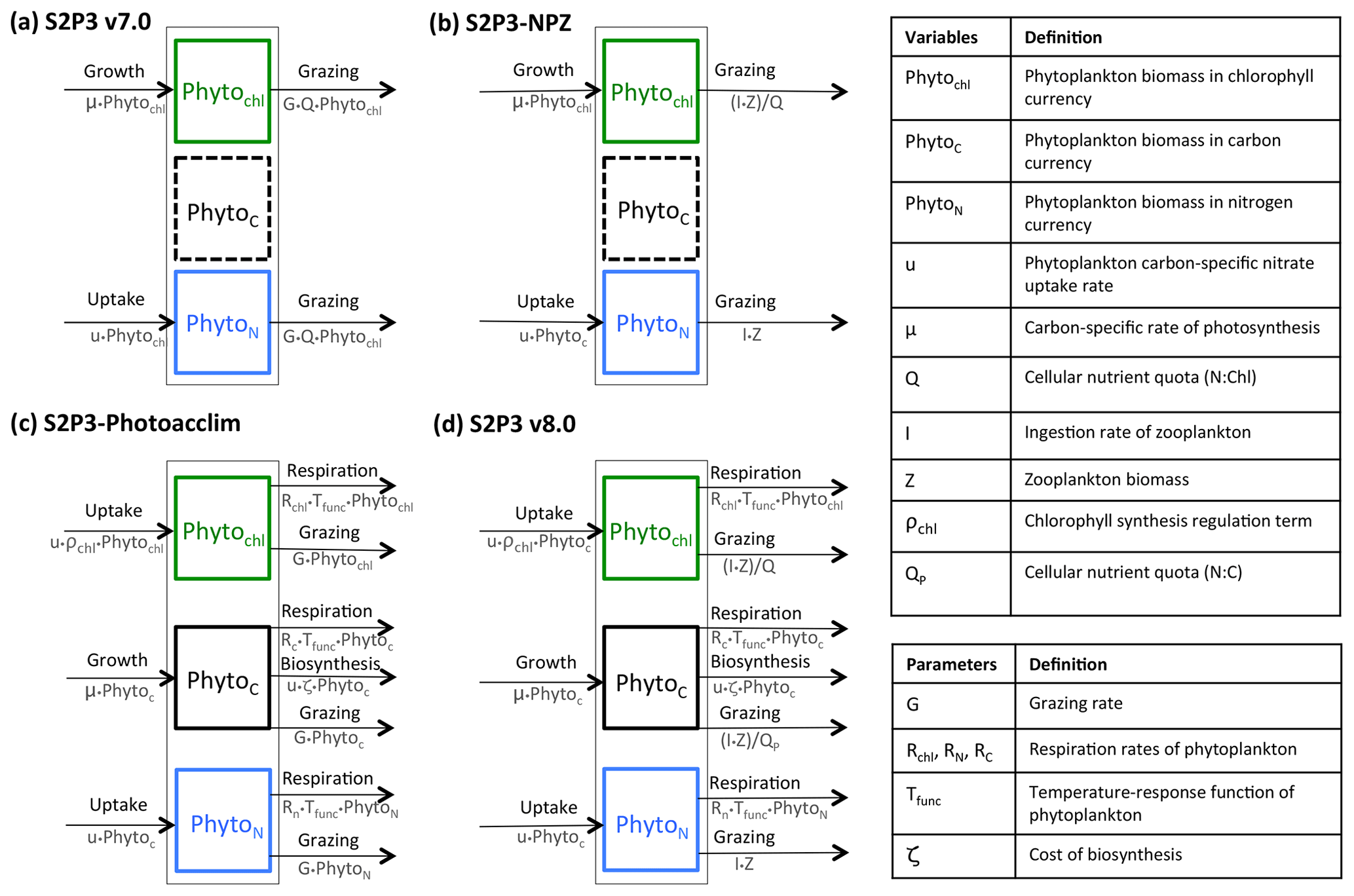
Figure 1Structure of the phytoplankton growth formulations: (a) S2P3 v7.0 model, with constant PhytoN : PhytoChl ratio (Q); (b) S2P3-NPZ model, including explicit zooplankton with an associated ingestion rate of phytoplankton (I) based on the Ivlev grazing type; (c) S2P3-Photoacclim model, with varying ratios of N : C : Chl, with phytoplankton chlorophyll content regulated by a coefficient of chlorophyll synthesis (ρChl), which reflects the ratio of energy assimilated to energy absorbed (Geider et al., 1996), and with phytoplankton carbon regulated through a cost associated with biosynthesis (uζ) (Vries et al., 1974; Geider, 1992; Geider et al., 1998), respiration, and grazing (G); (d) the S2P3 v8.0 model, including two different varying quotas for PhytoN : Phytoc and PhytoN : PhytoChl.
The S2P3 v7.0 model can be divided into two different components: a physical part and a biological part. For this research, the model is an improved version of the original described in Sharples et al. (2006) to be compiled and executed in a Unix environment (Marsh et al., 2015), allowing a 1-D representation of physical and biological processes in shelf seas by simulating the seasonal cycle of phytoplankton, water column stratification, and PP at a selected location defined by water depth and tidal current amplitude. The physical part of the model has been greatly described in many other studies (Sharples, 1999, 2008; Sharples et al., 2006; Simpson and Sharples, 2012; Marsh et al., 2015) and is not described in this section again. This model uses the turbulence closure scheme based on Canuto et al. (2001). Likewise, the biological part of the S2P3 v7.0 model is described in Marsh et al. (2015) (Fig. 1a).
In order to explicitly account for the influence of zooplankton grazing, and hence predator–prey dynamics, the S2P3 v7.0 model (Sharples et al., 2006; Marsh et al., 2015) is developed into an NPZ framework. This new version of the model (S2P3-NPZ) includes zooplankton as a state variable, contrary to the S2P3 v7.0 model where grazing (G) is calculated as a fixed seasonal cycle represented as a sink term in the phytoplankton tendency equation. Addition of an explicit grazer also allows comparison to zooplankton biomass observations. As within S2P3 v7.0, the biological part of the S2P3-NPZ model calculates phytoplankton biomass in chlorophyll currency (PhytoChl; mg Chl m−3). Similar to the S2P3 v7.0 model, the growth of phytoplankton biomass (μ) can be either nutrient limited or temperature limited, with the maximum growth rate of phytoplankton being related to temperature through an Eppley function and being modified by a nutrient quota (Q), which corresponds to a varying ratio between phytoplankton nitrogen and phytoplankton chlorophyll biomass (). Additionally, phytoplankton are modelled in terms of nitrogen (mmol N m−3) represented by PhytoN. Zooplankton biomass and external DIN are likewise modelled in terms of nitrogen (mmol N m−3; Fig. 1b).
The S2P3-Photoacclim model is a new version of the S2P3 v7.0 model, incorporating a more complete representation of phytoplankton physiology (Geider et al., 1998). This model allows phytoplankton to acclimate to changes in light and nutrients; therefore, the ratios of N : C : Chl and characteristics of phytoplankton physiology can vary, allowing direct comparison to physiological data. The biological part of the S2P3-Photoacclim model uses three currencies of phytoplankton biomass: carbon (PhytoC; mg C m−3), nitrogen (PhytoN; mg N m−3), and chlorophyll (PhytoChl; mg Chl m−3). The S2P3-Photoacclim model calculates phytoplankton growth as a function of both nitrogen assimilation and carbon fixation (i.e. variable Chl : N and Chl : C ratios). It is assumed that respiration (R) is equal for all cellular components as a function of temperature: , where Rref (d−1) is a degradation rate constant at a reference temperature (Fig. 1c).
The S2P3 v8.0 model describes a combination of zooplankton and physiological acclimation components in order to provide a more realistic representation of the ecosystem dynamics (Fig. 1d). This model can be divided into two different components: a physical part and a biological part. Full details and model equations of the biological part of the model are described below. Details of the variables and parameters are listed in Appendix A.
The biological part of the S2P3 v8.0 model calculates changes in phytoplankton carbon biomass (PhytoC) over time as
where μ is the growth rate of phytoplankton, RC is a respiration rate constant of phytoplankton, Tfunc is a temperature-response function of phytoplankton, u is the phytoplankton carbon-specific nitrate uptake rate, ζ is the cost of biosynthesis, I is the ingestion rate of zooplankton, and QP is the cellular nutrient : carbon quota.
Phytoplankton biomass is also modelled in terms of internal nitrogen, PhytoN. S2P3 v8.0 calculates PhytoN as
where Rn is the nitrate remineralisation constant.
The rate of change of phytoplankton biomass in terms of chlorophyll (PhytoChl) is described by
where ρChl is a chlorophyll synthesis regulation term, RChl is the chlorophyll degradation rate constant, and Q is the cellular nutrient quota (N : Chl).
The change in time of external DIN is calculated as
where γ1 is the grazing inefficiency or “messy feeding” that returns a fraction of grazed material back into the DIN pool, γ2 is the fraction of dead zooplankton that goes into the sediments, and m is the loss rate of zooplankton due to predation and physiological death.
Zooplankton grazing on phytoplankton response depends on a Holling type 2 or Ivlev grazing (Franks, 2002), with the ingestion rate of zooplankton (I) described as
where Rmax is the zooplankton maximal grazing rate (d−1) and λ is the rate at which saturation is achieved with increasing food levels (mmol N m−3)−1.
Zooplankton biomass is therefore modelled as
The carbon-specific, light-saturated photosynthetic rate depends on the internal nitrogen of phytoplankton described as a factor f based on the work of Moore et al. (2001):
where is the maximum value of the carbon-specific rate of photosynthesis and the factor f is defined as
Nitrogen assimilation is calculated as a saturating function of external nutrient content, the internal nutrient quota and the maximum nitrogen assimilation rate (umax) according to (Geider et al., 1998; Moore et al., 2001)
where kn is the half-saturation constant for nitrate uptake.
The carbon-specific photosynthesis is a saturating function of irradiance and it is calculated as
where αChl is the chlorophyll-specific initial slope of the photosynthesis–light curve, θ is the cellular chlorophyll : phytoplankton carbon ratio, and IPAR is the photosynthetically available radiation.
Finally, chlorophyll a synthesis depends on the rates of photosynthesis and light absorption:
where is the maximum value of the cellular chlorophyll : phytoplankton nitrogen ratio.
To calibrate or tune each model, they were adjusted on a trial-and-error basis until disagreement with the in situ observations was minimised, allowing investigation of the sensitivity of each model to changes in the parameters listed in Table 1.
4.1 UK SSB programme
Time series of surface chlorophyll a concentrations (mg Chl m−3) from long-term mooring deployments including the Carbon and Nutrient Dynamics and Fluxes over Shelf Systems (CaNDyFloSS) Smartbuoy (Mills et al., 2003) were collected at the CCS location (49.4∘ N, 8.6∘ W; depth of 145.8 m), gathering data for 5 min every 30 min during the years 2014 and 2015 as part of the research cruise expeditions DY029 and DY033. The phytoplankton community fluorescence from the water samples was calculated as a proxy for chlorophyll a and calibrated taking into account daytime fluorescence quenching which results in a reduction of fluorescence per unit chlorophyll. For this study, daytime data were removed.
Conductivity–temperature–depth (CTD) casts were performed in different locations on the NW European shelf from the CCS location to the shelf break, with discrete samples of temperature, DIN, and chlorophyll a collected using Niskin bottles as part of the research cruise expeditions DY029 and DY033. At the CCS location, the CTD samples were collected from pre-dawn to midday with a 1 m vertical resolution over the whole water column (140 m depth) during the year 2015. CTD casts for the CCS location were chosen to validate the model during spring and summer. Relevant information about dates and positions from other CTD casts taken during spring and summer of the year 2015 is listed in Table A1. CTD casts chosen to compare the each model are marked in bold in Table B1.
4.2 Zooplankton biomass
Zooplankton biomass samples were collected at the CCS location (49∘25 N, 8∘35 W; ∼150 m water depth) during four periods: 5–12 August, 10–29 November 2014, 3–28 April, and 13–31 July 2015 for the cruises DY026, DY018, DY029, and DY033, respectively (Giering et al., 2018). Zooplankton were fractionated into microplankton, small mesozooplankton, and large mesozooplankton by using different mesh sizes. For zooplankton biomass samples, net rings of 57 cm diameter were used and fitted with two different mesh sizes of 63 and 200 µm. The nets had a closing mechanism when deployed, sampling zooplankton biomass during daytime and nighttime at different depths: above and below the thermocline, and, when present, across the deep chlorophyll maximum (DCM; determined based on fluorescence measurements). The thermocline and DCM were determined from CTD casts immediately prior to the net deployments. The 63 and 200 µm mesh nets were hauled at 0.2 and 0.5 m s−1, respectively.
For the S2P3-NPZ and the S2P3 v8.0 models, only mesozooplankton biomass were considered, with a community composition that included amphipods, appendicularian, Chaetognatha, copepods, Euphausiacea, Polychaeta, and others (e.g. cladocerans, dinoflagellates, echinoderm, eggs, foraminifera, Gymnosomata, unidentified larvae, nauplii, ostracods, and radiolarian, all of which contributed <3 % in all samples). A FlowCam (Fluid Imaging Technologies Inc.) and a ZooScan were used to scan zooplankton individuals with images processed using ZooProcess 7.19 and Plankton Identifier 1.3.4 software (Gorsky et al., 2010). From these images, biovolume spectra were calculated and converted into image-derived dry weight (DW). The total 246 net hauls collected for biomass samples provided 44 vertical depth profiles, integrating zooplankton biomass typically between 0 and 120 m at the CCS location. The complete dataset can be obtained from the British Oceanographic Data Centre (BODC; http://www.bodc.ac.uk/data, last access: December 2019.) as reported in Giering et al. (2018).
4.3 Physiological observations
Water samples were collected in the Celtic Sea from cruises JR98 and CD173 using 10 L Niskin bottles for four of the sites (CS1, CS2, CS3, and IS1) (Fig. 2) during 24 h periods on 31 July, 29 July, 5 August, and 2 August, respectively. Multiple samples were collected at the surface and in deeper layers (in the surface mixed layer (SML) and the DCM) to obtain different phytoplankton populations throughout the photoperiod. The JR98 cruise was undertaken from 24 July to 14 August of 2003. Stations, from the Irish Sea to the Celtic Sea shelf break, ranged in characteristics from very strong, narrow thermoclines in the southern Celtic Sea (CS1), to the weak, deep surface layer associated with internal wave mixing at the shelf edge (CS2). On the other hand, the CD173 cruise was undertaken from 15 July to 6 August of 2005, from the stratified region of the Celtic Sea shelf (stations D2, CS1, CS3, U2) and shelf break (stations CS2, N1). For this work, observations from both cruises were used, considering only the stations from the seasonally stratified sites (B2, CS1, CS3, D2, JB1, OB, P1, U2, and ctd16) and excluding stations CS2 and N1 which are close to the shelf edge where advective fluxes are more relevant than in the stations closer to the CCS location and none of the models used here consider advective fluxes.
Photosynthesis vs. irradiance (P vs. E) experiments were conducted in short-term incubations (2–4 h) using a photosynthetron (Moore et al., 2006). From these P vs. E experiments, chlorophyll a normalised PP was derived from 14C uptake to obtain the chlorophyll a specific maximum light-saturated photosynthesis rate (mg C (mg Chl a)−1 h−1) and the maximum light utilisation coefficient, αChl (mg C (mg Chl a)−1 h−1 (µE m−2 s−1)−1) (Jassby and Platt, 1976; Hickman et al., 2012). Values of αChl and the light saturation parameter, Ek (µE m−2 s−1) (given by ) were spectrally corrected to the in situ irradiance at the sample depth according to the phytoplankton light absorption (Moore et al., 2006). The maximum light utilisation coefficient (αChl) was constrained for the S2P3-Photoacclim and the S2P3 v8.0 models by finding the mean from all observations: mg C (mg Chl a)−1 h−1 (µE m−2 s (ranges of this parameter accounted from to mg C (mg Chl a)−1 h−1 (µE m−2 s; SD ), and therefore the values of and Ek were used as variables for comparison with equivalent modelled values.
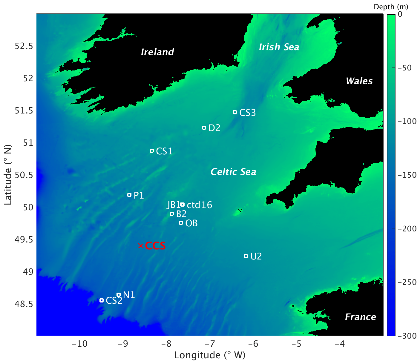
Figure 2Map of study area and stations for the JR98 and CD173 cruises, including the CCS location (in red colour). The image was created with MATLAB using the repository data for gridded bathymetry provided by General Bathymetric Chart of the Oceans (GEBCO). Bathymetric data are only considered for the shelf sea region (0 to 300 m depth) with open ocean depth neglected (deeper than 300 m). Continents considered in black colour (over 0 m elevation).
Table 1List of parameter values, including units and definitions for the calibrated S2P3-NPZ, S2P3-Photoacclim, and S2P3 v8.0 models.

4.4 Model calibration
For this study, approximately 2 years of phytoplankton chlorophyll data were available for the CCS location, while in the case of the zooplankton biomass observations, these were collected only during certain days per year allowing only a discrete representation of the seasonal cycle of zooplankton. Finally, profiles of physiological data were only collected during summertime of the years 2003 and 2005. The calibrated version of the S2P3-NPZ model shows differences in the timing of the spring phytoplankton bloom for the year 2015 in comparison to observations of surface chlorophyll (Fig. 3a), with a later bloom from the S2P3-NPZ model, reaching a peak bloom about a month later. Additionally, the magnitude of the spring phytoplankton bloom is also higher in the model in comparison to observations. Phytoplankton are able to escape grazing control in April and early May, with the spring zooplankton bloom occurring about a month later (Fig. 3b). Similar differences can be observed between the calibrated S2P3-Photoacclim model, demonstrating that constraining the timing of the spring phytoplankton bloom is a complex process. Tuning model parameters to generate earlier blooms modifies the magnitude of the spring phytoplankton bloom by increasing it to unrealistic levels. Figure 3 shows that between the three models the best agreement found in comparison to buoy observations correspond to the S2P3 v8.0 model, although the timing and magnitude of the spring phytoplankton bloom show some remaining small differences, with higher concentrations of surface chlorophyll a during spring (∼10 mg Chl m−3). Moreover, the timing of the spring phytoplankton bloom during the year 2014 matches the observations but a delayed bloom is shown during the year 2015. On the other hand, zooplankton biomass is higher than in the S2P3-NPZ and the predator–prey relationship is well represented, with the spring zooplankton bloom happening approximately a month later than the spring phytoplankton bloom during the year 2014, but this difference is lower during the year 2015, with the start of the zooplankton bloom happening about half a month after the start of the spring phytoplankton bloom. Remaining mismatches between the calibrated models and observations may be driven by water column processes including advection and diffusion that were not considered in these 1-D models but affects the real water column where the observations were taken. Furthermore, photo-acclimation and grazing depend on changes in temperature (Geider, 1987; Vázquez-Domínguez et al., 2013) and other ecosystem processes which are not explicitly represented, potentially explaining remaining mismatches between the observations and the calibrated S2P3 v8.0 model.
To provide a quantitative index of bloom timing, we consider a threshold criterion (Siegel et al., 2002; Greve et al., 2005; Fleming and Kaitala, 2006; Henson et al., 2009). In this study, the spring phytoplankton bloom is defined as when surface chlorophyll reaches more than 1.5 mg Chl m−3 (see Table B2). For the S2P3-Photoacclim model in comparison to CTD cast during spring (Fig. 4b), the model has not yet reached the spring phytoplankton bloom, whereas observations indicate the spring phytoplankton bloom has already started; the S2P3-Photoacclim model shows low chlorophyll a concentrations at the surface, with DIN concentrations not being depleted at this stage (Fig. 4c). Similar results can be seen for the S2P3-NPZ, although Table B2 shows that the spring phytoplankton bloom has already started in this model, but it is still later than in the observations. The S2P3 v8.0 model, on the contrary, shows a better agreement in terms of the timing of the spring phytoplankton bloom with the CTD observations. During summer months, the models are able to reproduce the subsurface mixed layer observed in the CTD profile (Fig. 4e) with a similar magnitude but shallower by approximately 20 m. On the other hand, the physical structure of the model shows good agreement with the observations during spring (Fig. 4a), but there are differences during summer (Fig. 4d). The lack of a marked mixed layer depth in all the models is likely related to short-term meteorology forcing: during 24 July 2015, the air temperature was high (∼20 ∘C) and wind speed was low (∼5 m s−1). However, the thermocline shows a sharp development in the CTD observations that cannot be constrained better in the models by parameterising values of the turbulent closure scheme, light attenuation in the water column, and mixing control parameters (data not shown).
The S2P3-Photoacclim and the S2P3 v8.0 models were further compared with phytoplankton physiological variability observations (Fig. 5). Figure 5 shows that near the sea surface, where light levels are high, photo-acclimation of phytoplankton, values of and Ek are higher than in deeper layers of the water column. The observed ranges approximately 0.5–2.5 × 10⁻³ (mg C (mg Chl a)−1 s−1) in the surface waters (first 5 m), while this range is smaller in deeper layers (0–1.0 mg C (mg Chl a)−1 s−1), e.g. at 40 m depth. Similar variability can be observed with Ek, having lower values in deeper layers of the water column, but the largest variability occurs in the surface layer (∼ 100–250 µE m−2 s−1). The S2P3-Photoacclim and S2P3 v8.0 models show good agreement with the observations, with plausible values of and Ek found through the water column particularly in terms of the magnitude of the vertical gradients. However, the version of the S2P3 v8.0 model which has the best parameterisations when tuned to fit the timing of the spring bloom has remaining discrepancies when compared to the physiological observations, showing an overestimation of and Ek at depth. Calibration of these models against physiological data is relatively novel as such comparisons remain rare. Greater complexity allowed the S2P3 v8.0 model to resolve a more diverse range of biogeochemical dynamics, explicitly accounting for zooplankton biomass and for the dynamics of internal quotas of phytoplanktonic cells, with phytoplankton biomass being in carbon, nitrogen, and chlorophyll currencies, allowing the decoupling of nutrient uptake from carbon fixation (Klausmeier et al., 2004; Flynn, 2008; Bougaran et al., 2010; Bernard, 2011; Mairet et al., 2011; Ayata et al., 2013). Including additional parameters in models can add more unconstrained degrees of freedom (Ward et al., 2010) but also allows for more parameter combinations and therefore more flexibility to constrain S2P3 v8.0 in order to reproduce observations. The new added parameters and variables in the S2P3 v8.0 model, were carefully chosen to allow the model to be constrained against additional data, specifically zooplankton abundances and photosynthetic physiological measurements; therefore, a higher complexity allowed better representations of the temporal dynamics. Additionally, despite having more sophisticated formulations of the ecosystem, the S2P3 v8.0 model continues to be a 1-D model, allowing multiple experiments to be run at the same time with relatively low computational cost.
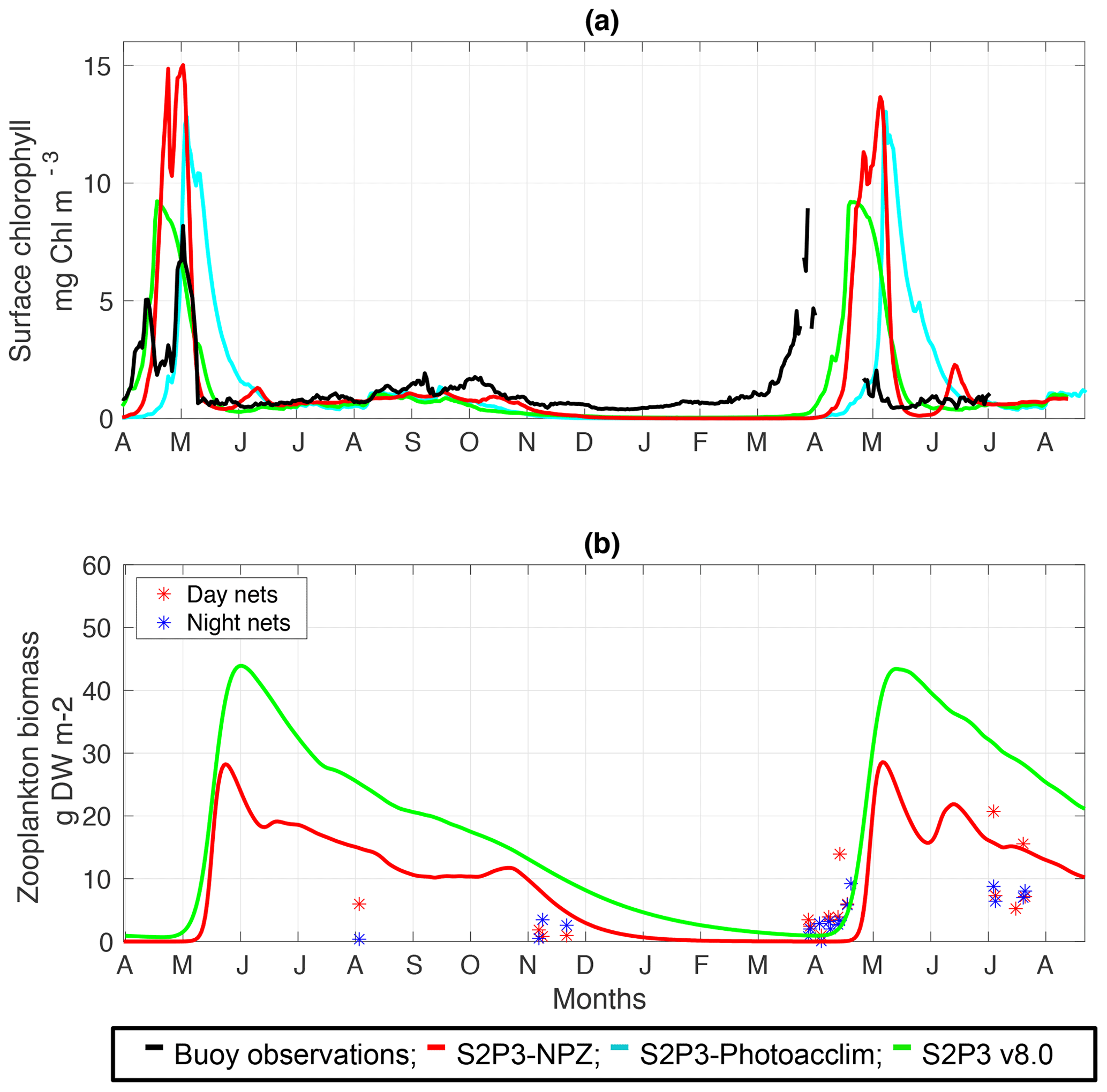
Figure 3(a) SSB observations of surface chlorophyll a (black line), along with the modelled surface chlorophyll a for the S2P3-NPZ (red line), S2P3-Photoacclim (cyan line), and S2P3 v8.0 (green line) calibrated models. (b) Observations of zooplankton biomass presented as discrete points for day nets (red dots) and night nets (blue dots) taken during the cruises DY026, DY018, DY029, and DY033; modelled zooplankton biomass from the S2P3-NPZ (red line) and S2P3 v8.0 (green line) calibrated models.
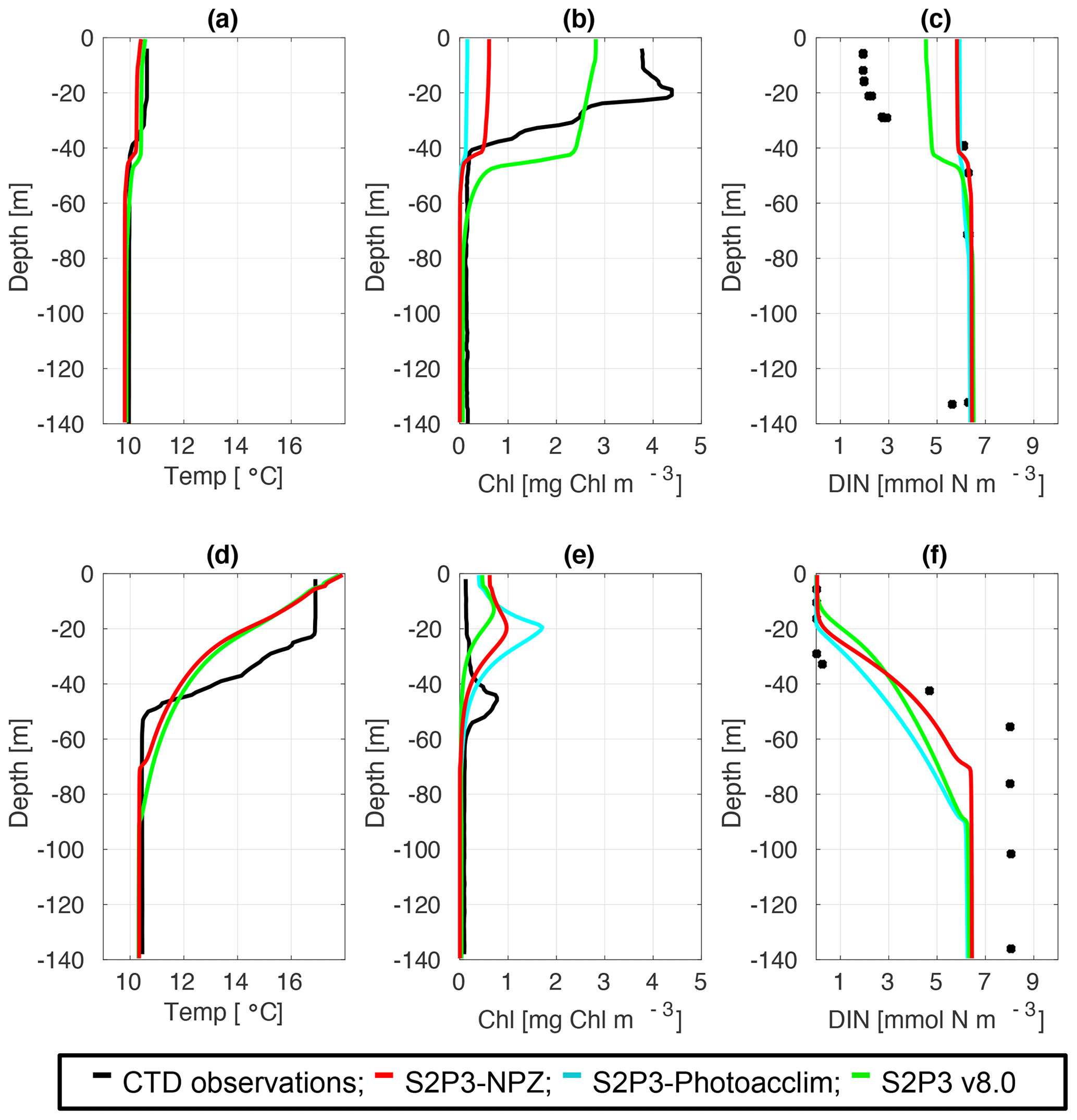
Figure 4CTD observations from the SSB programme (black lines) including data for springtime (20 April 2015) (a) temperature, (b) chlorophyll a, and (c) DIN (black dots); for summertime (24 July 2015) (d) temperature, (e) chlorophyll a, and (f) DIN (black dots) along the S2P3-NPZ (red line), S2P3-Photoacclim (cyan line), and S2P3 v8.0 (green line) calibrated models.
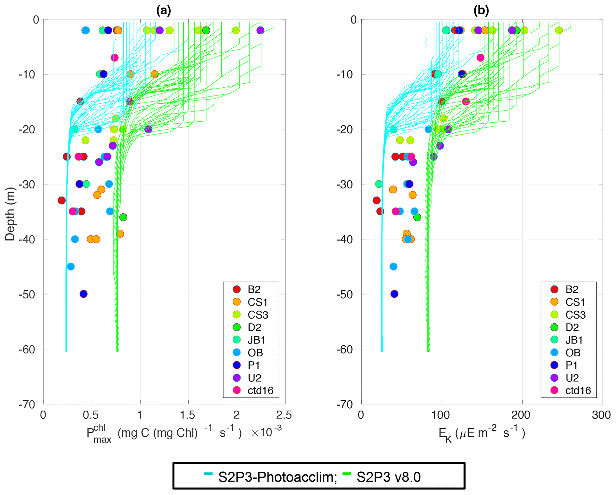
Figure 5Observations from the cruises CD173 and JR98 for (a) chlorophyll a specific maximum light-saturated photosynthesis rate in different locations in the Celtic Sea and for the calibrated S2P3-Photoacclim model (cyan lines) and the S2P3 v8.0 model (green lines); (b) observations of the light saturation parameter (Ek) for different stations across the Celtic Sea and for the calibrated S2P3-Photoacclim model (cyan lines) and the S2P3 v8.0 model (green lines). The data from both models were plotted for the same days that the observations were collected.
The behaviour of the S2P3 v8.0 model calibrated for the CCS location is displayed in Figs. 6 and 7. Figure 6 shows contour plots from daily profiles of the S2P3 v8.0 model for temperature (Fig. 6a), phytoplankton chlorophyll a (Fig. 6b), zooplankton biomass (Fig. 6c), phytoplankton chlorophyll : phytoplankton carbon ratio (Fig. 6d), and DIN (Fig. 6e) for the years 2014 and 2015 which correspond to the observation period of the SSB programme. Figure 6 allows a more detailed overview of the model dynamics. Water column temperature increases from April of each year, reaching a maximum value at the surface during summer months. At the same time, the spring phytoplankton bloom can be observed during April, reaching ∼10 mg Chl m−3. Additionally, the spring zooplankton bloom can be observed approximately a month after the spring phytoplankton bloom is developed, with zooplankton being able to grow during summer months and decreasing until a minimum value during winter. These spring blooms also mark the start of DIN depletion at the surface, a state that lasts until the end of summer. Finally, the phytoplankton chlorophyll : phytoplankton carbon ratio shows the highest values during winter months when irradiance levels are low, with the Chl : N ratio decreasing until the end of summer due to the lower concentrations of chlorophyll in the cell to avoid internal damage due to high irradiance during this period, highlighting the photo-acclimation of phytoplankton and flexible stoichiometry of the S2P3 v8.0 model.
Figure 7 provides a general overview of the dynamics of the calibrated S2P3 v8.0 model, representing the interannual variability of each variable using the median (black lines), and lower and upper quantiles (red lines; 95 % of the data distribution) during 1965 to 2015. Figure 7a shows the start of thermal stratification during early spring with observable interannual variability in the extent of stratification. Once the water column is stratified, the spring phytoplankton bloom can be observed (Fig. 7b), followed by the start of the spring zooplankton bloom (Fig. 7c). As phytoplankton grow, DIN concentrations at the surface start to deplete reaching a minimum value during spring and summer months, and increasing when thermal stratification breaks down during winter months (Fig. 7d). Finally, net primary production (NPP) time series show seasonal and interannual phytoplankton dynamics (Fig. 7e). All variables of the S2P3 v8.0 model shown in Fig. 7 provide the spectrum of interannual variability of 95 % of the data using the upper and lower quantile values (red lines), demonstrating that the interannual variability of thermal stratification provides variability for the timing and magnitude of the spring phytoplankton bloom as well as summer growth.

Figure 6Contoured daily vertical profiles for the start of 2014 to the end of 2015 for the calibrated version of the S2P3 v8.0 model including (a) temperature (∘C), (b) phytoplankton chlorophyll a (mg Chl m−3), (c) zooplankton biomass (mmol N m−3), (d) phytoplankton chlorophyll : phytoplankton carbon ratio (mg Chl (mg C)−1), and (e) DIN (mmol N m−3).
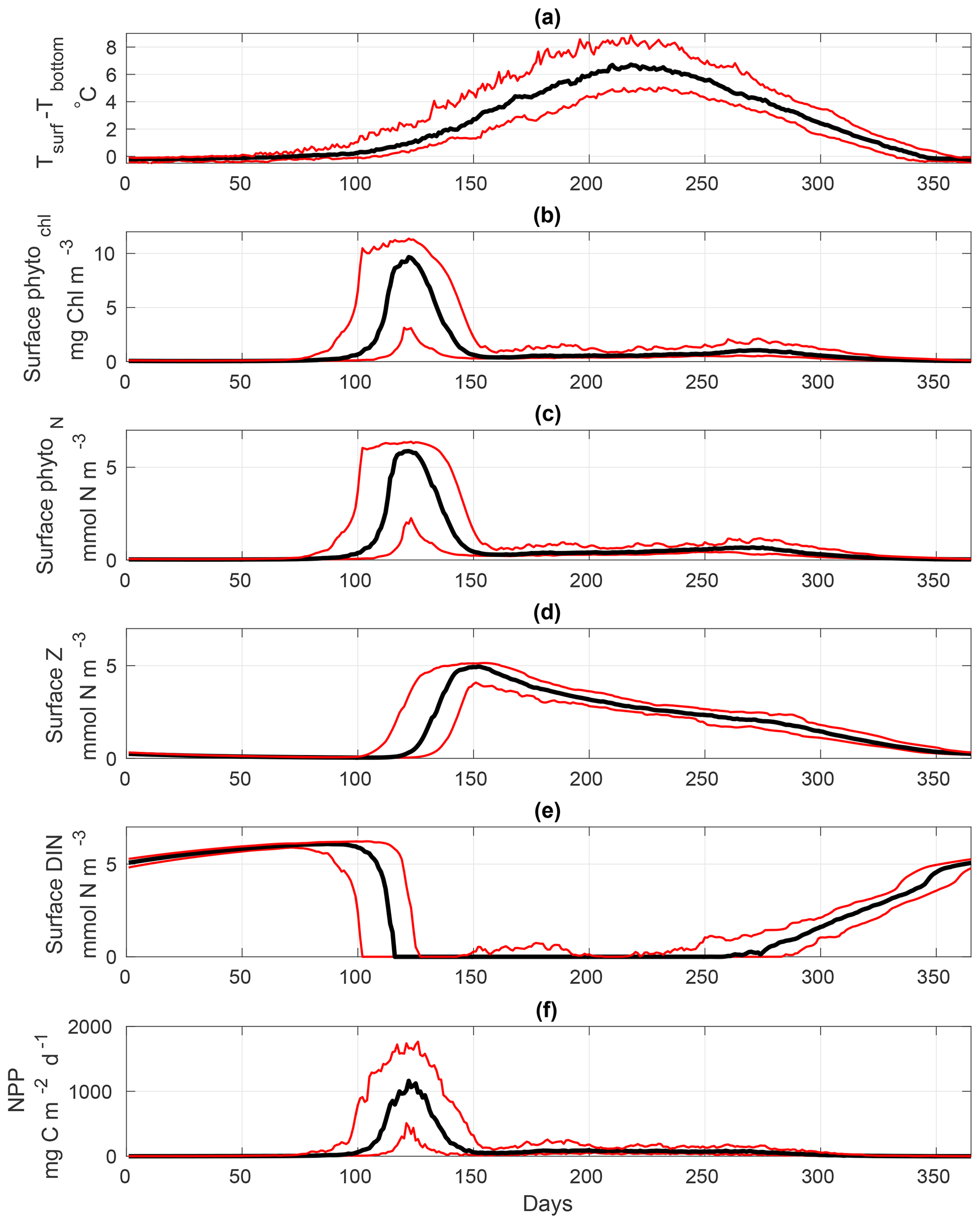
Figure 7Annual representation of the median (black lines) calculated from 1965 to 2015 for the S2P3 v8.0 model calibrated for the CCS location and forced with all meteorological components (i.e. wind speed, cloud coverage, air temperature, and relative humidity). Red lines represent the annual lower and upper quantiles for each variable of the model (95 % distribution of the data) over 1965–2015. (a) Surface temperature minus bottom temperature (∘C), (b) surface chlorophyll a (mg Chl m−3), (c) surface zooplankton biomass (mmol N m−3), (d) surface DIN (mmol N m−3), and (e) net primary production (NPP) (mg C m−2 d−1).
Table 2List of the most sensitive experiments run for the S2P3 v8.0 model calibrated for the CCS location, including the year of observations, timing and magnitude of the spring phytoplankton bloom, and total annual zooplankton biomass values.
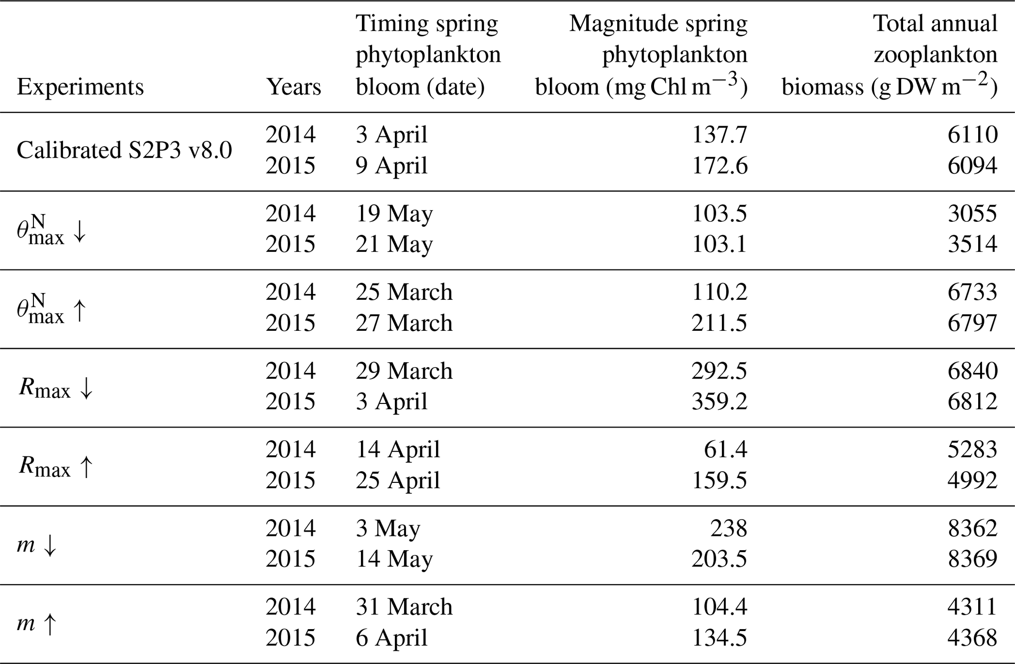
An analysis was performed to assess the sensitivity of the model to selected parameter values for the S2P3 v8.0 model. Each parameter listed in Table 1 was varied in turn in order to understand how sensitive the model is to those changes and the effect that they have on the modelled ecosystem dynamics at the CCS location. In each case, parameters were varied from the best calibrated value by +50 % and −50 %. Sensitivity studies are important tools to improve the accuracy of shelf sea models (Chen et al., 2013), but developing these analyses has to be done carefully in order to identify which processes are responsible for the observed model behaviour (Ward et al., 2013). A direct comparison was calculated in terms of the S2P3 v8.0 model attributes considering the timing and magnitude of the spring phytoplankton bloom, and the total annual zooplankton biomass for the calibrated version of the model and each experiment, providing better insights on the effects that each parameter produces in the behaviour of each model. Table 2 only shows the experiments involving the zooplankton maximal grazing rate (Rmax), mortality of zooplankton (m), and the maximum value of the Chl : N ratio (), as they were demonstrated to be the most significant parameters in terms of the sensitivity of the model according to the attributes calculated, with the rest of the experiments omitted for this discussion. The S2P3 v8.0 model is strongly influenced by NPZ parameters, with the zooplankton maximal grazing rate (Rmax) (Stegert et al., 2007) and zooplankton mortality rate (m) having the largest effect in the magnitude of the spring phytoplankton bloom (Figs. C1a, C4a) and in the total annual zooplankton biomass (Figs. C1b, C4b). The effect of Rmax implies that lower values in the maximum ingestion rate of phytoplankton can produce earlier and larger spring phytoplankton blooms compared to the calibrated S2P3 v8.0 model. On the other hand, a higher value of Rmax shows a delayed spring phytoplankton bloom (Fig. C2) compared to the CTD observations. Additionally, zooplankton mortality produced differences in the timing of the spring phytoplankton bloom, with delays of 30 d (year 2014) and 35 d (year 2015) when there is less zooplankton mortality, affecting the timing and magnitude of the spring zooplankton bloom, therefore generating low values of surface chlorophyll a during spring (Fig. C5). It is well known that zooplankton are key players in the biogeochemical cycling of carbon and nutrients in marine ecosystems (Beaugrand and Kirby, 2010; Beaugrand et al., 2010), influencing the export of organic matter to the deep ocean (González et al., 2009; Juul-Pedersen et al., 2010). Additionally, grazing responses comprise the dominant losses for phytoplankton in the ocean (Banse, 1994), influencing plankton stocks and primary production (Franks et al., 1986).
Table 2 presents differences for the S2P3 v8.0 model calibrated for the CCS location and for selected sensitivity experiments in terms of the timing of the spring phytoplankton bloom (days), defined as in Table B2, using a threshold for phytoplankton biomass (> 1.5 mg Chl m−3); the magnitude of the spring phytoplankton bloom (mg Chl m−3); and the total annual zooplankton biomass (g DW m−2). Representation of phytoplankton physiology had an important influence on the timing of the spring phytoplankton bloom (Table 2), with affecting the S2P3 v8.0 model the most in terms of this attribute of the model structure, showing less productive and delayed spring blooms when is lower (Figs. C7a, C8b). Changes in the timing and magnitude of the spring zooplankton bloom coincide with the changes of the timing and magnitude of the phytoplankton blooms (Fig. C7b). These changes in the plankton communities over the year due to different values of , also have an effect on the values of DIN (Fig. C8c, f), with the largest differences shown during springtime at the surface (Fig. C8c). These differences agree with the results found by Ayata et al. (2013), where it was demonstrated that taking into account photo-acclimation and variable stoichiometry of phytoplankton growth in marine ecosystem models produces qualitative and quantitative differences in phytoplankton dynamics. Moreover, these quota formulations in S2P3 v8.0 were compared to the available dataset of physiological observations (Fig. C9). It is interesting to note that the sensitivity analysis of NPZ parameters produced differences in the physiological variables and Ek, specially at the surface (Figs. C3, C6), suggesting that the predator–prey interactions are indirectly influencing phytoplankton physiology, presumably through feedbacks between zooplankton and the nutrient cycling, which subsequently have an effect on phytoplankton physiology due to the dependency of nutrient quotas to the availability of inorganic nutrients. The current study thus demonstrates how a greater variety of data, spanning multiple trophic levels and incorporating information on physiological status as well as standing stocks, provides additional constraints on model validation and hence constraints on parameterisation.
Table 3Comparison between the S2P3 v7.0, S2P3-NPZ, S2P3-Photoacclim, and S2P3 v8.0 models calibrated for the CCS location, in terms of the total spring NPP, total summer NPP, and total annual NPP calculated from 1965 to 2015, including the mean, maximum, minimum, and SD values.
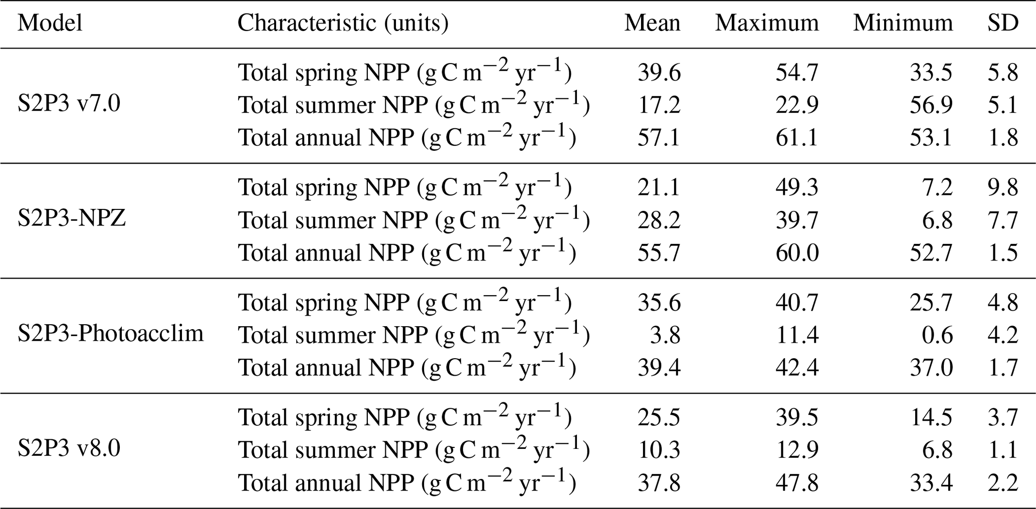
The S2P3 v7.0 (Sharples et al., 2006; Marsh et al., 2015), S2P3-NPZ, S2P3-Photoacclim, and S2P3 v8.0 models were calibrated for the CCS location and further analysis was undertaken by running each model for a extended period (1965–2015) to evaluate the statistics of productivity, partitioned between spring and summer. Table 3 shows that for the S2P3 v7.0 model, on average, 69.2 % of the annual phytoplankton production occurs during the spring phytoplankton bloom. On the other hand, for the S2P3-NPZ model, on average, only 37.8 % of the annual production occurs during spring months, showing that the predator–prey relationship has a strong influence on the magnitude of the spring phytoplankton bloom every year. Additionally, the S2P3-Photoacclim model shows a very strong spring phytoplankton bloom, corresponding to 90 % of the total annual NPP. Finally, for the S2P3 v8.0 model, only 67.4 % of the annual production corresponds to the spring bloom period. It is clear that, on average, the least productive model overall was S2P3 v8.0, followed by the S2P3-NPZ, S2P3 v7.0, and S2P3-Photoacclim. This shows the impact and complexity that the predator–prey relationship has on the model dynamics, with the addition of explicit zooplankton and their grazing activity as one of the main losses of phytoplankton (Franks et al., 1986). On the other hand, the S2P3 v7.0 model has, on average, more total annual NPP than the S2P3-NPZ model, suggesting that the influence of a constant grazing rate is not as strong in comparison to the one provided by the zooplankton grazing (NPZ framework), because the predator–prey relationship cannot be entirely represented in the S2P3 v7.0 model.
This study demonstrates that the combination of an NPZ framework, photo-acclimation, and flexible stoichiometry of phytoplankton in one model produces a better representation of the ecosystem based on the comparison to observations. This combined framework offers an improvement to the S2P3 v7.0 model for application to the CCS location and more broadly within shelf sea systems. The model validation, using both zooplankton biomass and physiological rates of phytoplankton observations, is rarely found in the literature, providing a novel contribution to the marine biogeochemistry modelling field of shelf seas. The development of the S2P3 v8.0 model provides a better fit to observations in comparison to the S2P3 v7.0, S2P3-NPZ, and S2P3-Photoacclim models. Improved confidence in the S2P3 v8.0 model thus suggests improved insights in studies about the effects of physical forcing through tides (Sharples, 2008), intra- and interannual variations in meteorology (Sharples et al., 2006) and other drivers on PP, and phytoplankton dynamics would be possible.
Appropriate parameterisations to represent shelf seas is a subject that should be further supported by fieldwork campaigns and future work should aim to include additional datasets with longer time series (Friedrichs et al., 2007; Ward et al., 2010). For this study, constraining the seasonal cycle of the phytoplankton physiology is not possible due to the lack of physiological observations during other periods of the year; furthermore, phytoplankton and zooplankton biomass datasets only include the years 2014 and 2015 but longer time series would help to improve the model calibration. Many model parameters quantities are poorly constrained observationally mainly due to the fact that model state variables are highly integrated pools, which are affected by biotic and abiotic factors in the environment, making them difficult to be determined by in situ measurements (Fennel et al., 2001).
The tuning and sensitivity analysis performed in this work allows a better understanding of the ecosystem dynamics represented in the model and how it is influenced by each parameter. By considering the timing and magnitude of the spring phytoplankton bloom, the annual zooplankton biomass, and summer phytoplankton photosynthetic physiology as features to be calculated, a quantitative and clearer comparison between each model could be developed. Finally, the model calibration will never be in perfect agreement with all the observations, particularly in this case, where only one type of phytoplankton and zooplankton was considered. Thus, responses must represent some typical or average dynamics and cannot represent any effects of competition between types. Additionally, no stages of zooplankton growth were taken into account, which might affect the predator–prey interactions (Wroblewski, 1982; Fennel, 2001). Despite such potential limitations, the S2P3 v8.0 model is able to reasonably represent the integrated behaviour of the mixture of species that inhabit the NW European shelf sea.
Table A1List of all variables for the biological part of the S2P3 v8.0 model.
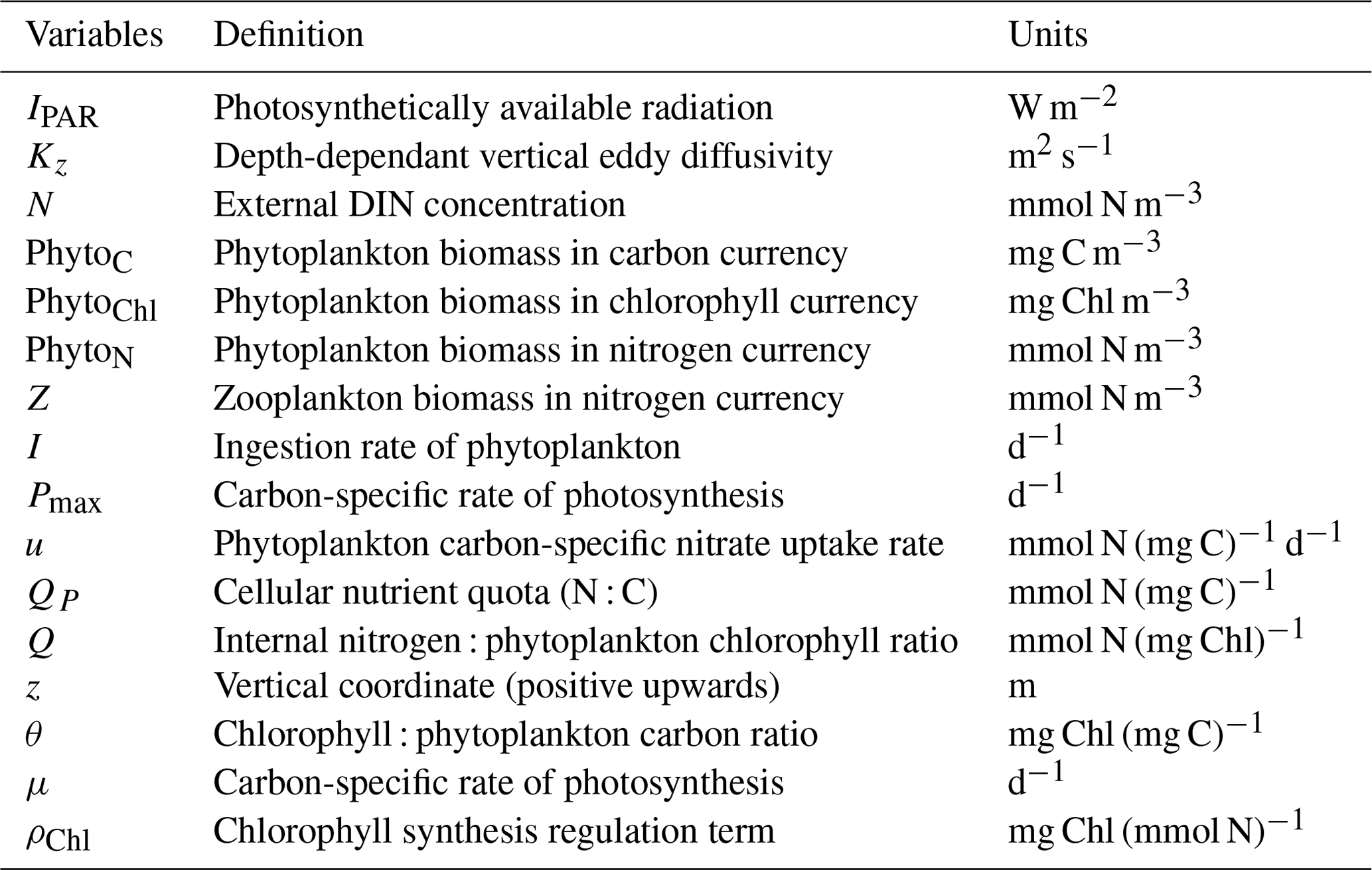
Table A2List of parameters, with their respective definitions, units, and initialised values for the biological part of the S2P3 v8.0 model.

Table B1List of relevant CTD casts for the CCS location from DY029 and DY033 cruises considering the date, location (latitude and longitude), and depth. CTD casts in bold are the ones chosen in this work to validate each model during spring and summer.

Table B2Quantitative comparison of the timing of the spring phytoplankton bloom between the buoy observations, S2P3-NPZ, S2P3-Photoacclim, and S2P3 v8.0 models.
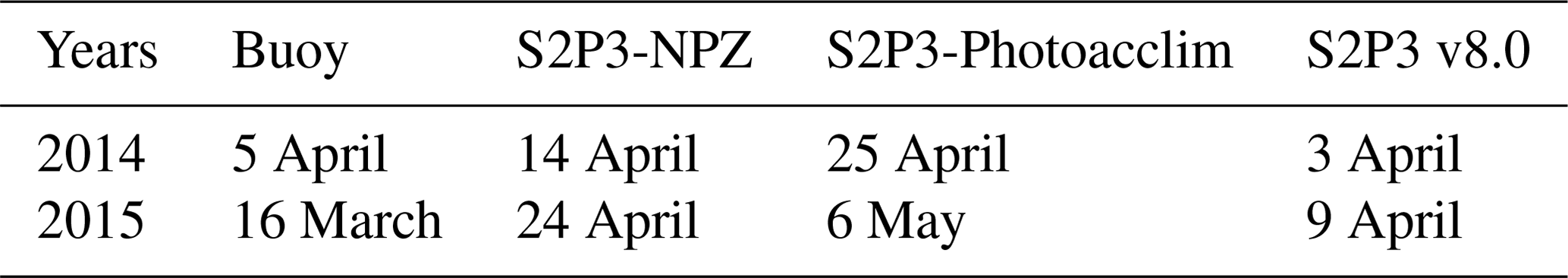
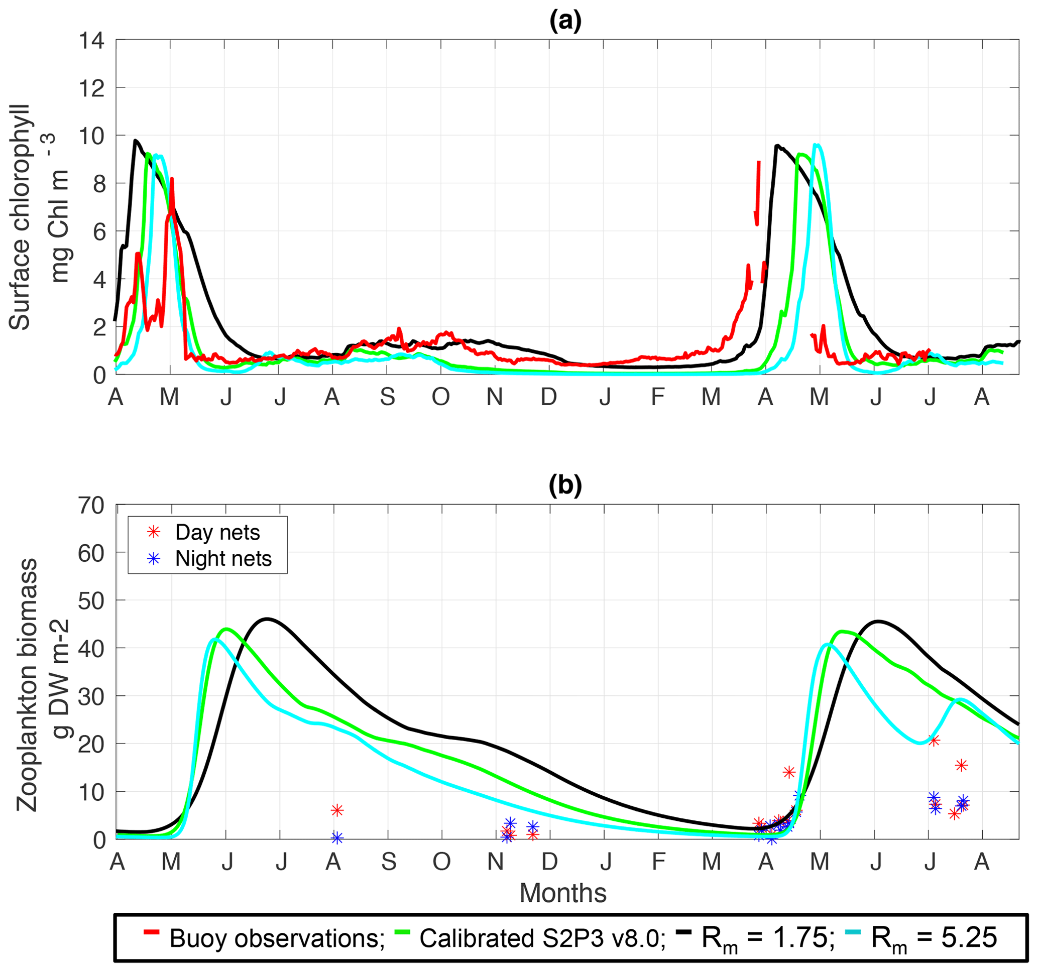
Figure C1(a) SSB observations of surface chlorophyll a (red line), along with the modelled surface chlorophyll a for the calibrated S2P3 v8.0 model (green line), and experiments Rmax=1.75 (black line) and Rmax=5.25 (cyan line). (b) Observations of zooplankton biomass presented as discrete points for day nets (red dots) and night nets (blue dots) taken during the cruises DY026, DY018, DY029, and DY033; modelled zooplankton biomass from the calibrated S2P3 v8.0 model (green line) and experiments Rmax=1.75 (black line) and Rmax=5.25 (cyan line).
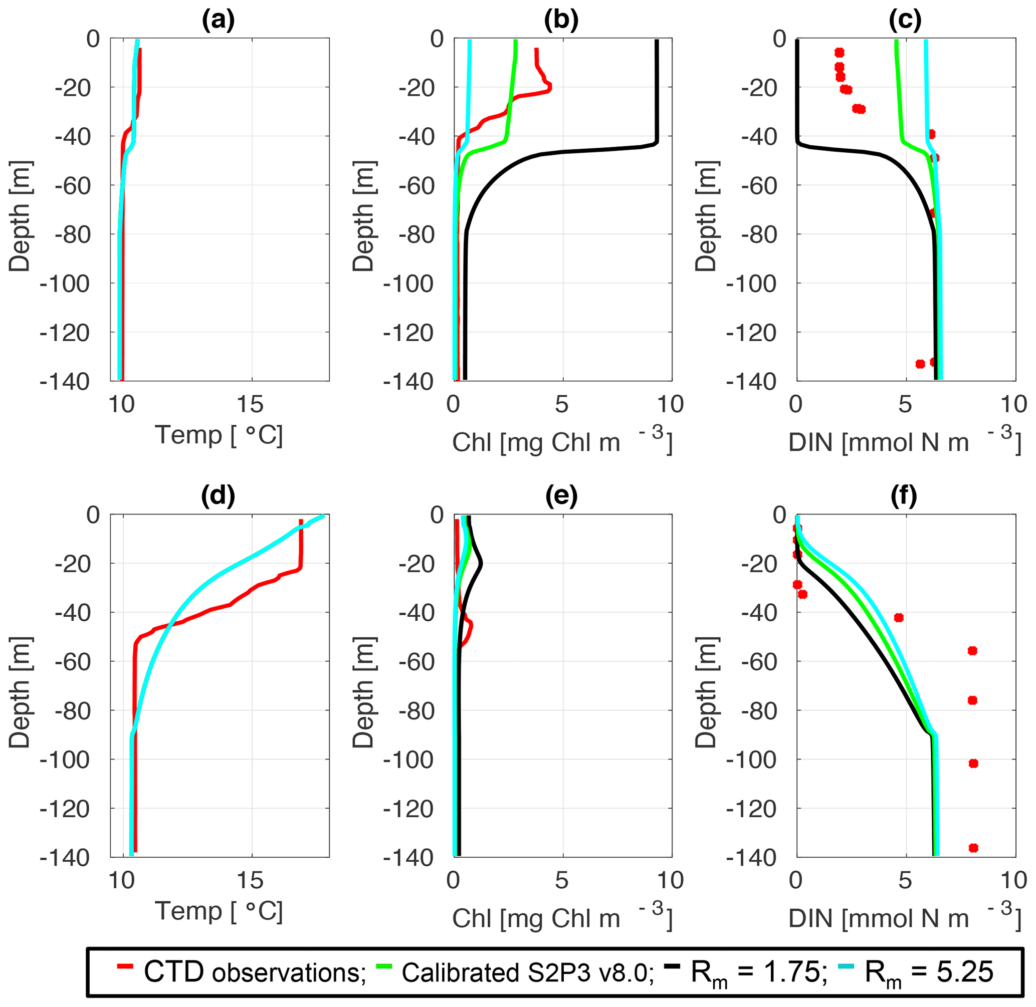
Figure C2CTD observations from the SSB programme (red line) including data for springtime (20 April 2015) (a) temperature, (b) chlorophyll a, and (c) DIN (red dots); for summertime (24 July 2015) for (d) temperature, (e) chlorophyll a, and (f) DIN (red dots) along the calibrated S2P3 v8.0 model (green line), experiments Rmax=1.75 (black line) and Rmax=5.25 (cyan line).
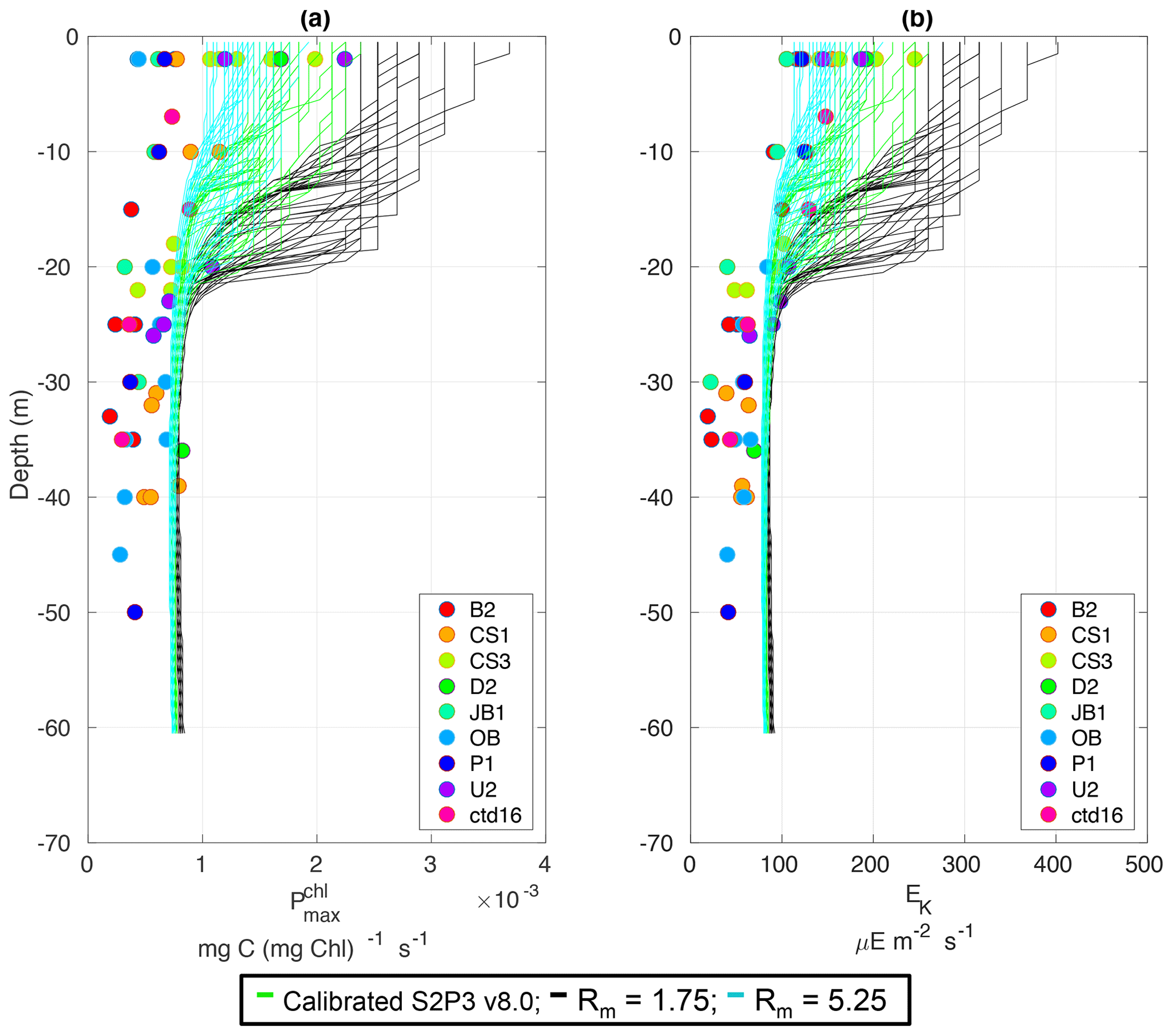
Figure C3Observations from the cruises CD173 and JR98 in different locations in the Celtic Sea, including the calibrated S2P3 v8.0 model (green lines), experiments Rmax=1.75 (black lines) and Rmax=5.25 (cyan lines) for (a) chlorophyll a specific maximum light-saturated photosynthesis rate and (b) light saturation parameter (Ek).
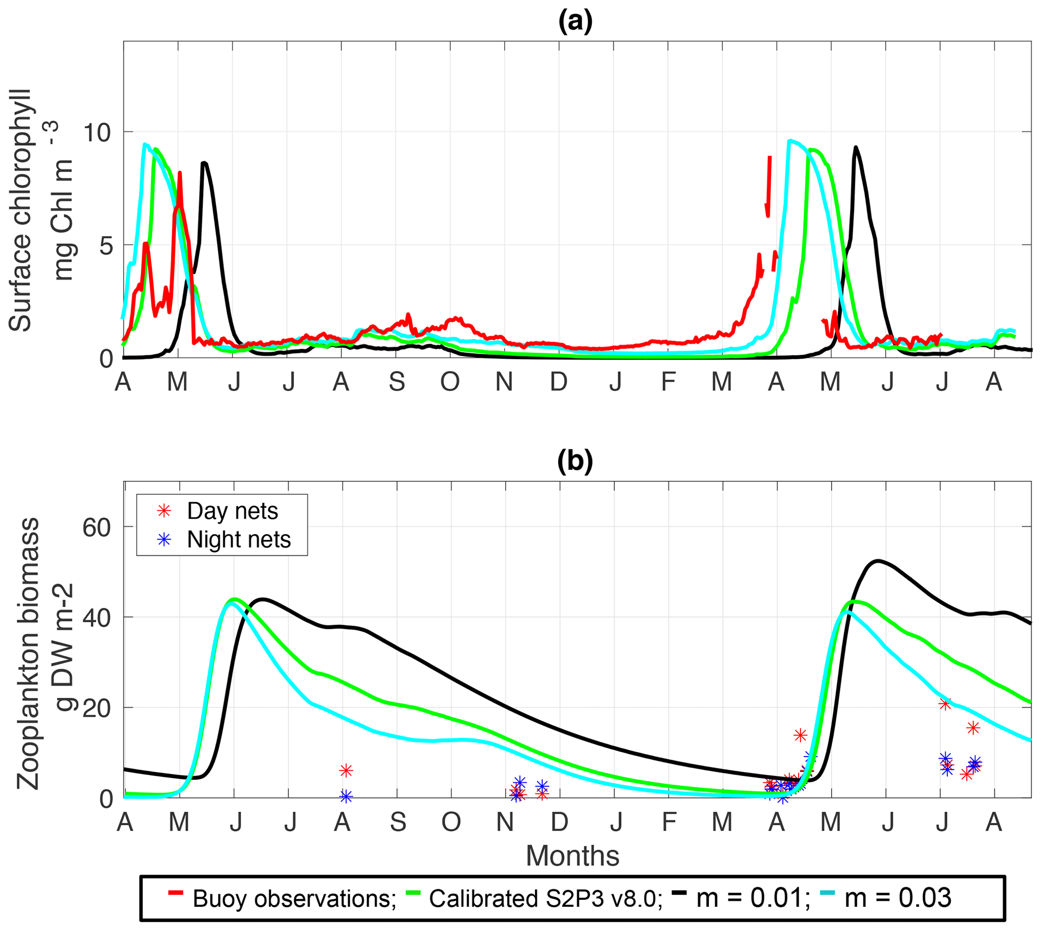
Figure C4(a) SSB observations of surface chlorophyll a (red line), along with the modelled surface chlorophyll a for the calibrated S2P3 v8.0 model (green line), and experiments m=0.01 (black line) and m=0.03 (cyan line). (b) Observations of zooplankton biomass presented as discrete points for day nets (red dots) and night nets (blue dots) taken during the cruises DY026, DY018, DY029, and DY033; modelled zooplankton biomass from the calibrated S2P3 v8.0 model (green line) and experiments m=0.01 (black line) and m=0.03 (cyan line).
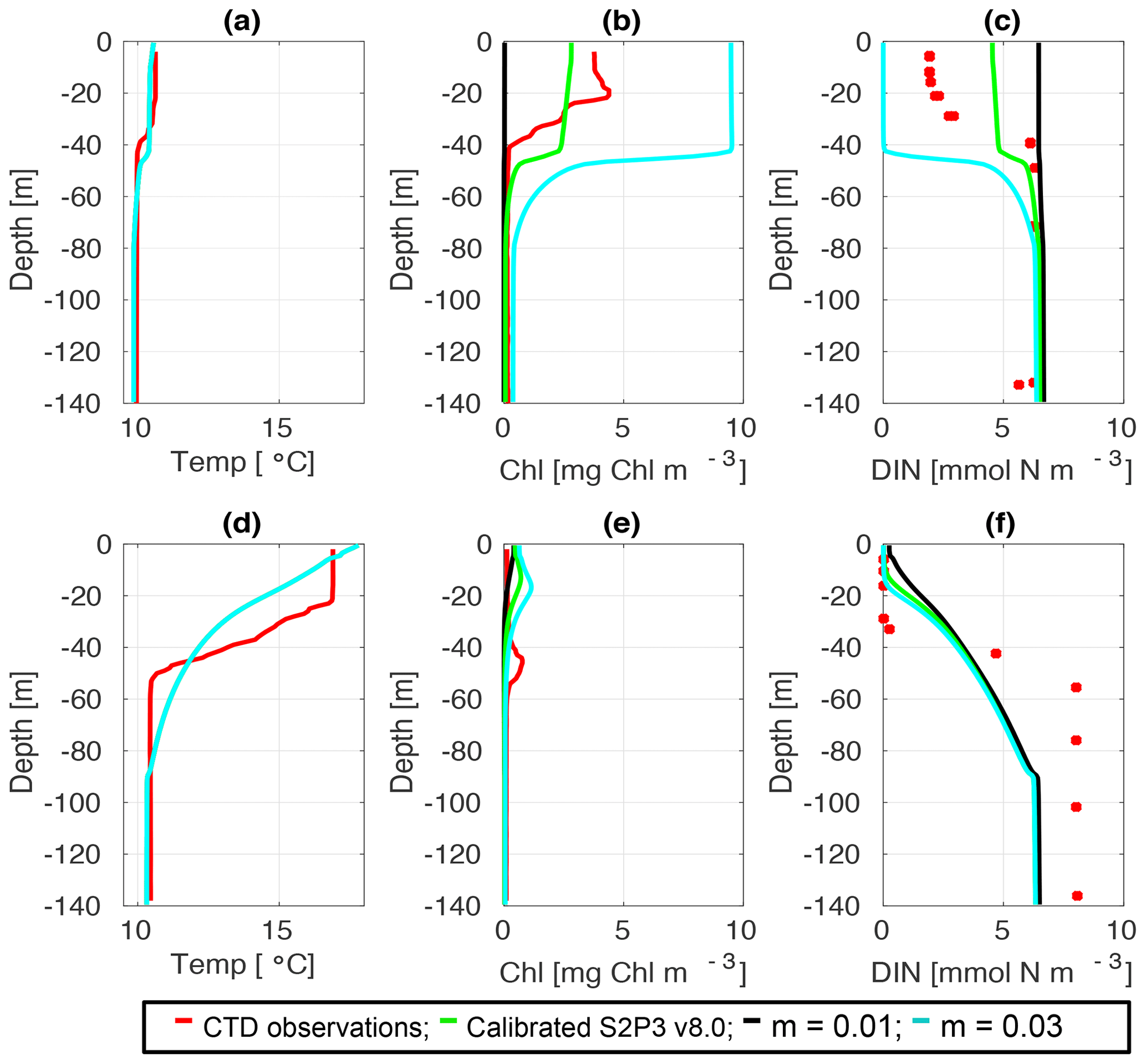
Figure C5CTD observations from the SSB programme (red line) including data for springtime (20 April 2015) (a) temperature, (b) chlorophyll a, and (c) DIN (red dots); for summertime (24 Jul 2015) for (d) temperature, (e) chlorophyll a, and (f) DIN (red dots) along the calibrated S2P3 v8.0 model (green line), experiments m=0.01 (black line) and m=0.03 (cyan line).
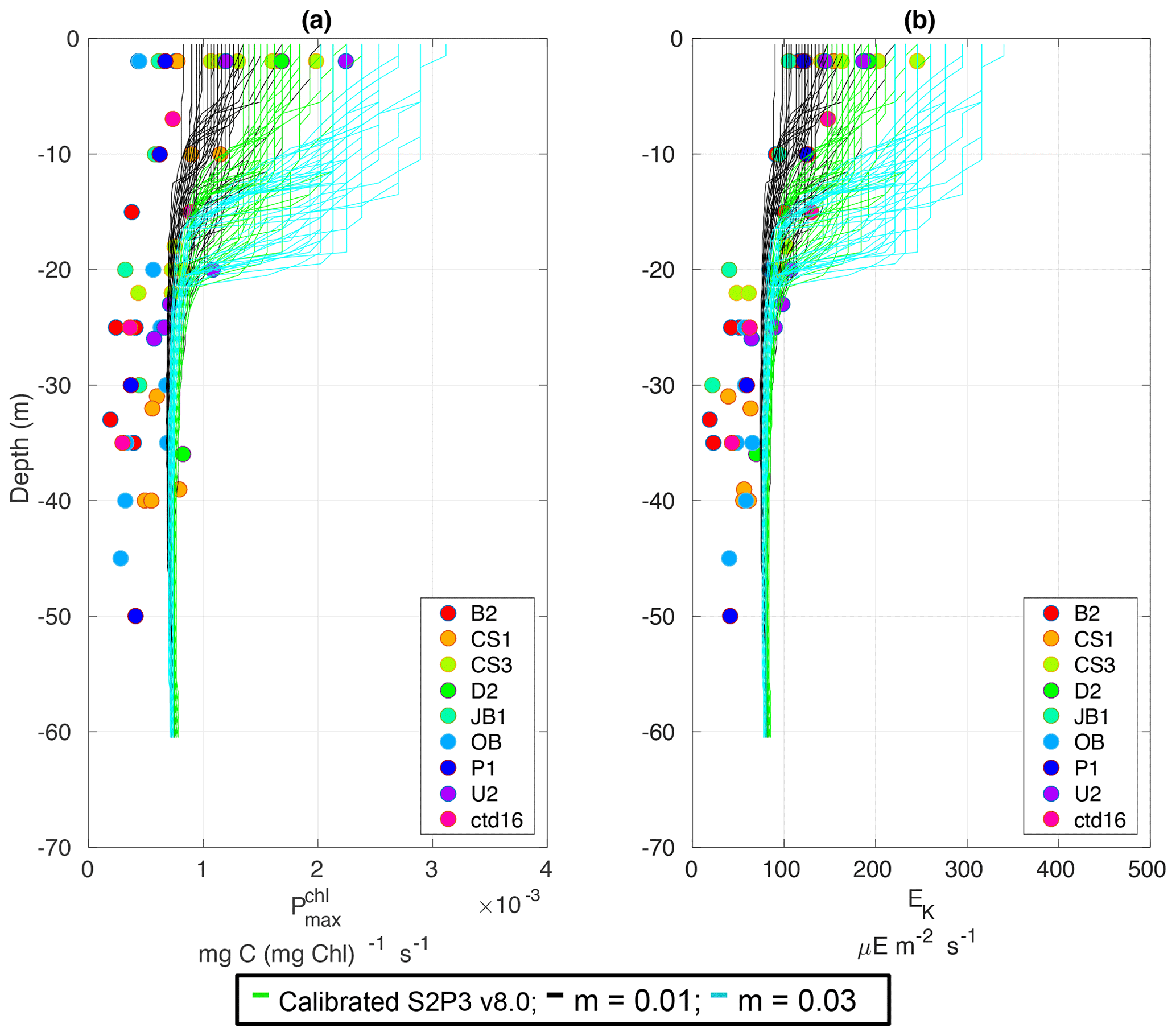
Figure C6Observations from the cruises CD173 and JR98 in different locations in the Celtic Sea, including the calibrated S2P3 v8.0 model (green lines), experiments m=0.01 (black lines) and m=0.03 (cyan lines) for (a) chlorophyll a specific maximum light-saturated photosynthesis rate () and (b) light saturation parameter (Ek).
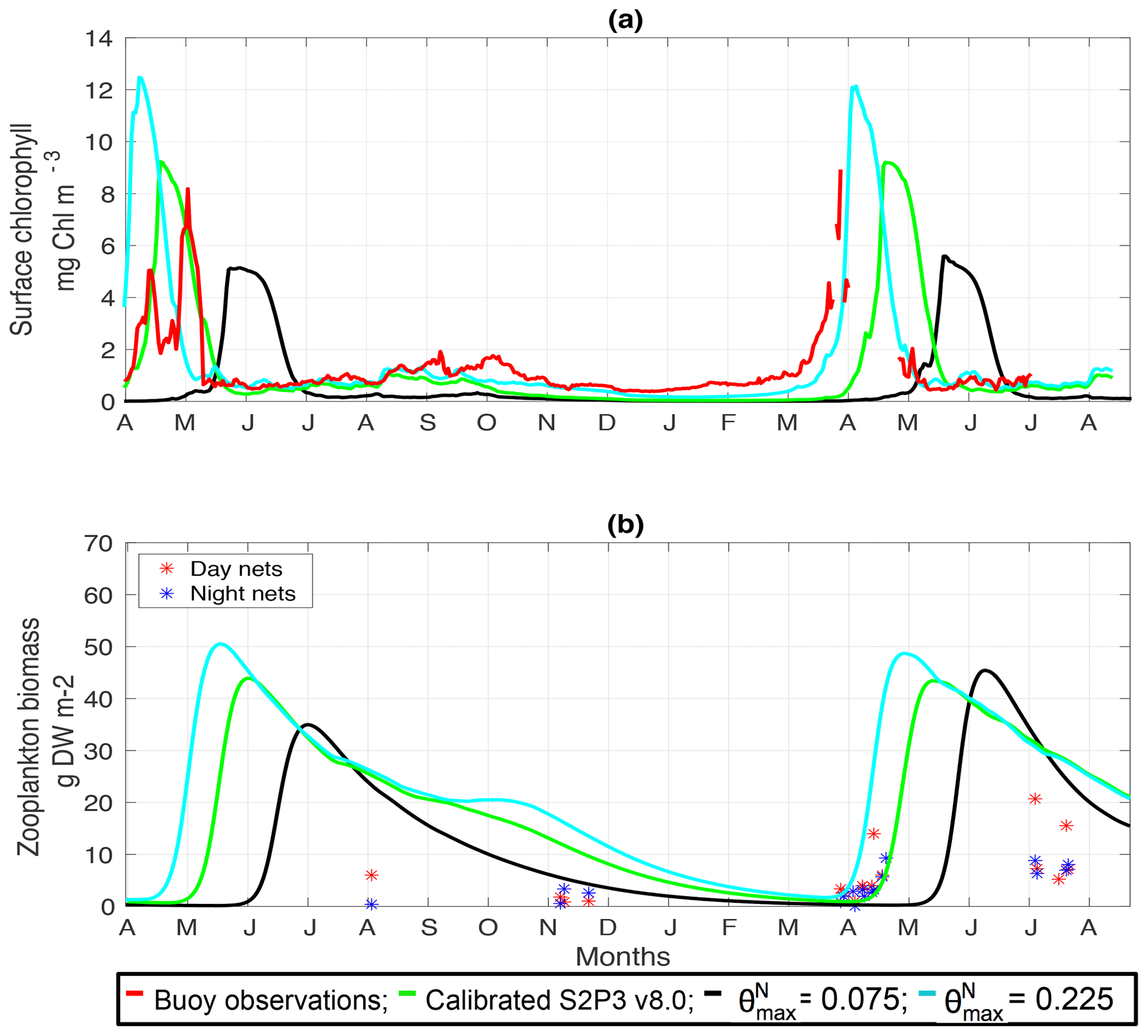
Figure C7(a) SSB observations of surface chlorophyll a (red line), along with the modelled surface chlorophyll a for the calibrated S2P3 v8.0 model (green line), and experiments (black line) and (cyan line). (b) Observations of zooplankton biomass presented as discrete points for day nets (red dots) and night nets (blue dots) taken during the cruises DY026, DY018, DY029, and DY033; modelled zooplankton biomass from the calibrated S2P3 v8.0 model (green line) and experiments (black line) and (cyan line).
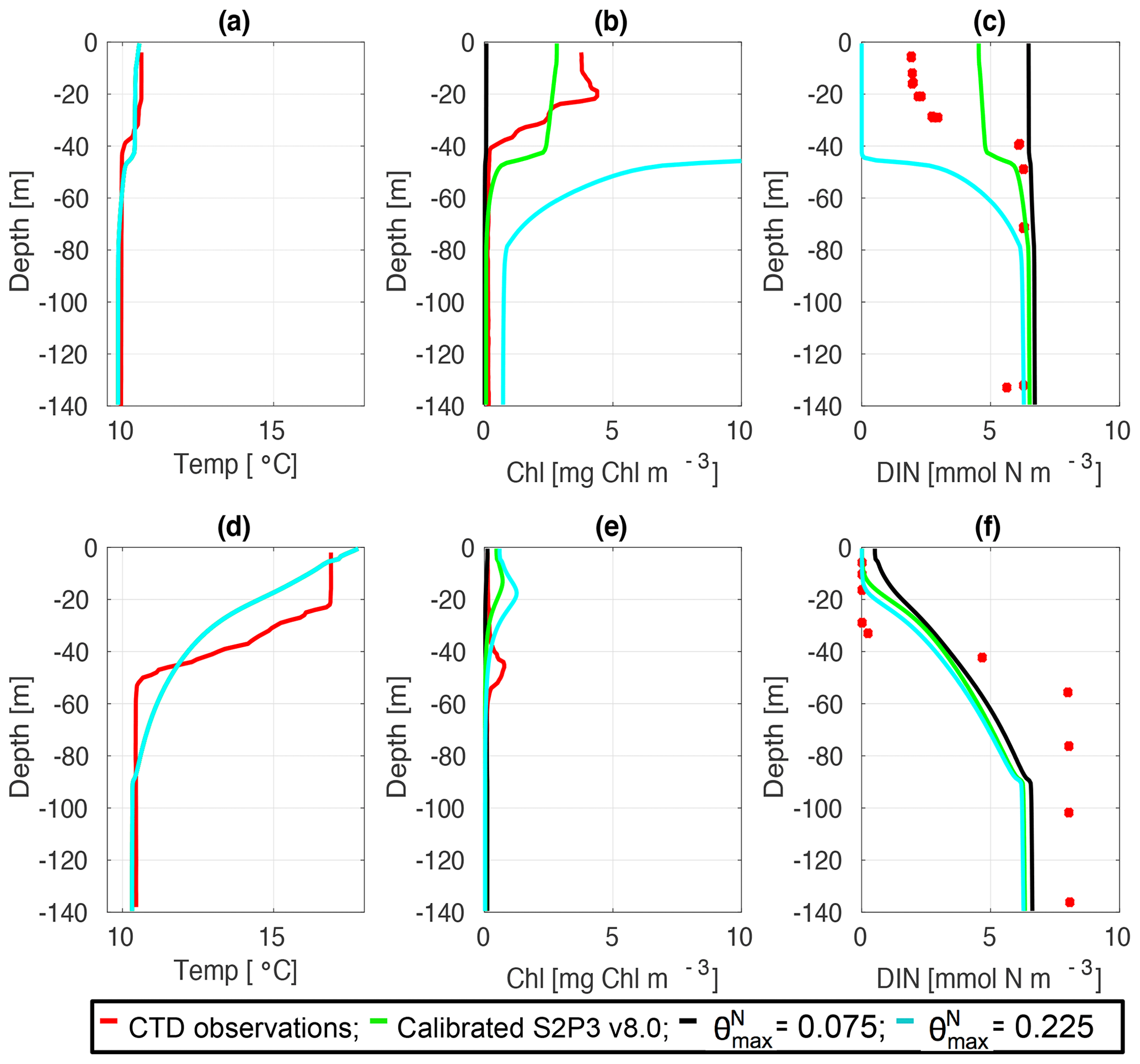
Figure C8CTD observations from the SSB programme (red line) including data for springtime (20 April 2015) (a) temperature, (b) chlorophyll a, and (c) DIN (red dots); for summertime (24 July 2015) for (d) temperature, (e) chlorophyll a, and (f) DIN (red dots) along the calibrated S2P3 v8.0 model (green line), experiments (black line) and (cyan line).
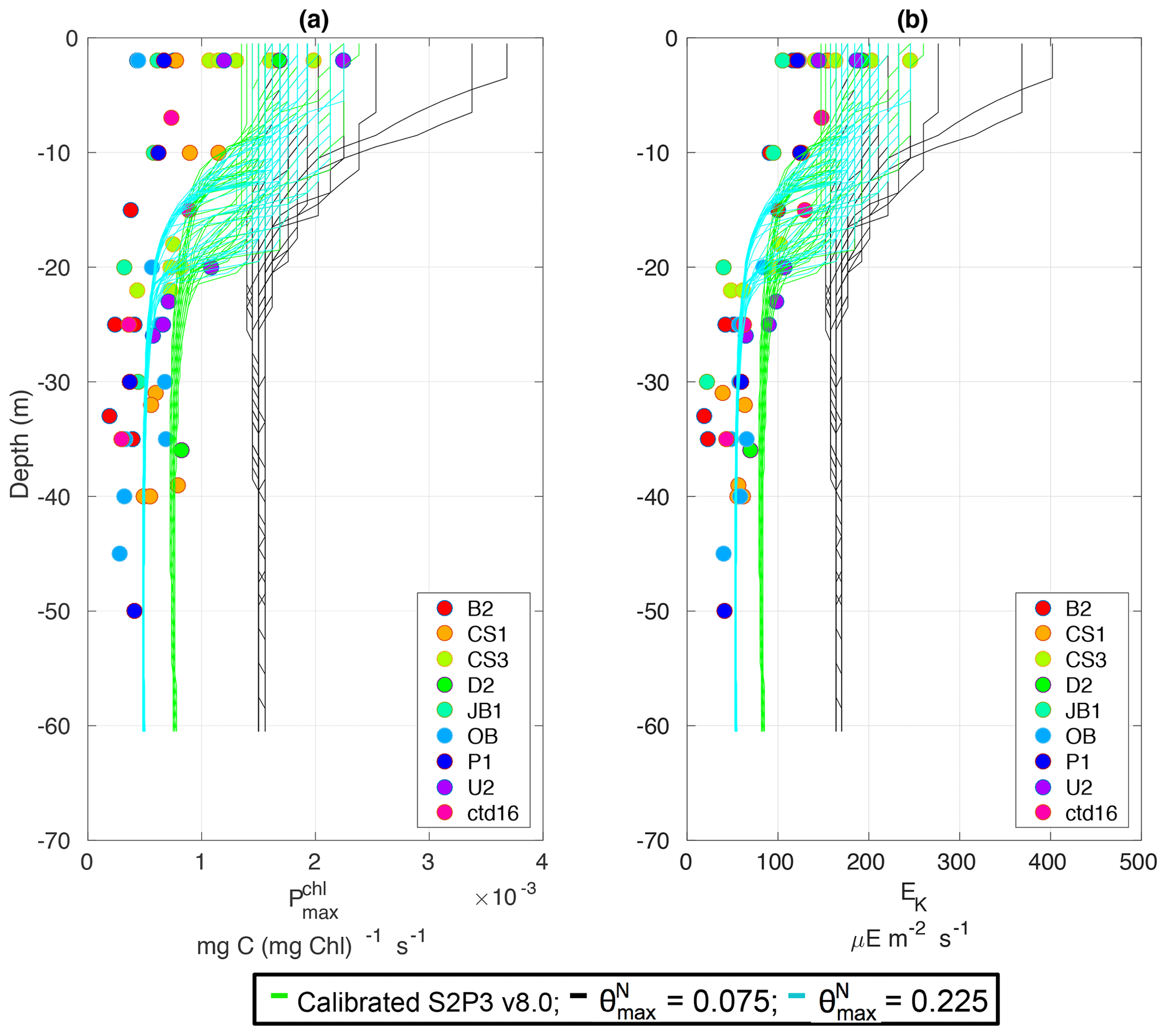
Figure C9Observations from the cruises CD173 and JR98 in different locations in the Celtic Sea, including the calibrated S2P3 v8.0 model (green lines), experiments (black lines) and (cyan lines) form (a) chlorophyll a specific maximum light-saturated photosynthesis rate and (b) light saturation parameter (Ek).
The current version of model is available from https://doi.org/10.5281/zenodo.3600467 (Bahamondes Dominguez et al., 2020) under the Creative Commons Attribution 4.0 international license. The exact version of the model used to produce the results used in this paper is archived on Zenodo (https://zenodo.org/record/3600467#.XyqbKhNKhBw, last access: 10 August 2020), as are input data and scripts to run the model and produce the plots for all the simulations presented in this paper.
Unzipped and uncompressed, the directory /s2p3v8.0 contains several subdirectories:
-
/main contains the source code, s2p3_v8.f90, which is compiled “stand-alone”, and executed using accompanying scripts.
-
/domain contains location (latitude and longitude), tidal components, and bathymetry (total depth) for the central Celtic Sea in the western English Channel (s12_m2_s2_n2_h_tim.dat).
-
/met contains 2000–2015 meteorological forcing (Falmouth_met_i143_j17_2000-2015 ASCII file).
-
/output contains example output data from experiments that show the calibrated version of each model (S2P3v8, S2P3-Photoacclim, and S2P3-NPZ).
-
/plotting contains MATLAB scripts for plotting time series data from experiments S2P3v8, S2P3-Photoacclim, and S2P3-NPZ. This folder also include all the datasets from observations used to validate each model.
The ancillary files needed for simulations are available on request from the author (e-mail: aab1g15@soton.ac.uk).
AABD developed the model code, performed the simulations, and prepared the manuscript with contributions from all co-authors.
The authors declare that they have no conflict of interest.
Hydrographic and biological observations used were acquired through the Natural Environment Research Council (NERC) funded UK Shelf Sea Biogeochemistry (SSB) research programme. Data used were requested from and are available from the British Oceanographic Data Centre (BODC). Sari Giering is thanked both for original collection and generation of the zooplankton data and discussion on interpretation of this data. NCEP/NCAR reanalysis 1 data were provided by the NOAA/OAR/ESRL PSD, Boulder, Colorado, USA, from their website at https://www.esrl.noaa.gov/psd/ (last access: December 2019). We thank the topical editor Paul Halloran and two anonymous reviewers for a series of insightful comments that helped to improve the manuscript.
This research has been supported by the CONICYT PFCHA/DOCTORADO BECAS CHILE/2015 (grant no. 72160249).
This paper was edited by Paul Halloran and reviewed by two anonymous referees.
Anderson, T. R.: Plankton functional type modelling: running before we can walk?, J. Plankton Res., 27, 1073–1081, 2005. a, b
Ayata, S. D., Levy, M., Aumont, O., Sciandra, A., Sainte-Marie, J., Tagliabue, A., and Bernard, O.: Phytoplankton growth formulation in marine ecosystem models: Should we take into account photo-acclimation and variable stoichiometry in oligotrophic areas?, J. Marine Syst., 125, 29–40, 2013. a, b
Bahamondes Dominguez, A., Hickman, A. E., Marsh, R., and Moore, C. M.: Constraining the response of phytoplankton to zooplankton grazing and photo-acclimation in a temperate shelf sea with a 1-D model – towards S2P3 v8.0 (Version 8.0), Zenodo, https://doi.org/10.5281/zenodo.3600467, 2020. a
Banse, K.: Grazing and Zooplankton Production as Key Controls of Phytoplankton Production in the Open Ocean, Oceanography, 7, 13–20, https://doi.org/10.5670/oceanog.1994.10, 1994. a
Beaugrand, G. and Kirby, R. R.: Climate, plankton and cod, Glob. Change Biol., 16, 1268–1280, https://doi.org/10.1111/j.1365-2486.2009.02063.x, 2010. a
Beaugrand, G., Edwards, M., and Legendre, L.: Marine biodiversity, ecosystem functioning, and carbon cycles, P. Natl. Acad. Sci. USA, 107, 10120–10124, https://doi.org/10.1073/pnas.0913855107, 2010. a
Bernard, O.: Hurdles and challenges for modelling and control of microalgae for CO2 mitigation and biofuel production, J. Process. Contr., 21, 1378–1389, https://doi.org/10.1016/j.jprocont.2011.07.012, 2011. a
Bougaran, G., Bernard, O., and Sciandra, A.: Modeling continuous cultures of microalgae colimited by nitrogen and phosphorus, J. Theor. Biology., 265, 443–454, https://doi.org/10.1016/j.jtbi.2010.04.018, 2010. a
Canuto, V., Howard, A., Cheng, Y., and Dubovikov, M.: Ocean Turbulence. Part I: One-Point Closure Model—Momentum and Heat Vertical Diffusivities, J. Phys. Oceanogr., 31, 1413–1426, https://doi.org/10.1175/1520-0485(2001)031<1413:OTPIOP>2.0.CO;2, 2001. a
Chen, C., Liu, H., and Beardsley, R.: An Unstructured Grid, Finite-Volume, Three-Dimensional, Primitive Equations Ocean Model: Application to Coastal Ocean and Estuaries, J. Atmos. Ocean. Tech., 20, 159–186, https://doi.org/10.1175/1520-0426(2003)020<0159:AUGFVT>2.0.CO;2, 2003. a
Chen, F., Shapiro, G., and Thain, R.: Sensitivity of Sea Surface Temperature Simulation by an Ocean Model to the Resolution of the Meteorological Forcing, ISRN Oceanography, 2013, https://doi.org/10.5402/2013/215715, 2013. a
Davis, C., Mahaffey, C., Wolff, G., and Sharples, J.: A storm in a shelf sea: Variation in phosphorus distribution and organic matter stoichiometry, Geophys. Res. Lett., 41, 8452–8459, https://doi.org/10.1002/2014GL061949, 2014. a
Droop, M. R.: 25 years of algal growth kinetics, Bot. Mar., 26, 99–112, 1983. a, b
Edwards, K. P., Barciela, R., and Butenschön, M.: Validation of the NEMO-ERSEM operational ecosystem model for the North West European Continental Shelf, Ocean Sci., 8, 983–1000, https://doi.org/10.5194/os-8-983-2012, 2012. a, b
Falkowski, P. and Laroche, J.: Acclimation to Spectral Irradiance in Algae, J. Phycol., 27, 8–14, https://doi.org/10.1111/j.0022-3646.1991.00008.x, 1991. a, b
Fennel, K., Losch, M., Schröter, J., and Wenzel, M.: Testing a marine ecosystem model: Sensitivity analysis and parameter optimization, J. Marine Syst., 28, 45–63, https://doi.org/10.1016/S0924-7963(00)00083-X, 2001. a
Fennel, W.: Modeling of copepods with links to circulation models, J. Plankton Res., 23, 1217–1232, https://doi.org/10.1093/plankt/23.11.1217, 2001. a
Fleming, V. and Kaitala, S.: Phytoplankton Spring Bloom Intensity Index for the Baltic Sea Estimated for the years 1992 to 2004, Hydrobiologia, 554, 57–65, https://doi.org/10.1007/s10750-005-1006-7, 2006. a
Flynn, K.: The importance of the form of the quota curve and control of non-limiting nutrient transport in phytoplankton models, J. Plankton Res., 30, 423–438, https://doi.org/10.1093/plankt/fbn007, 2008. a
Franks, P. J. S.: NPZ Models of Plankton Dynamics: Their Construction, Coupling to Physics, and Application, J. Oceanogr., 58, 379–387, https://doi.org/10.1023/A:1015874028196, 2002. a, b
Franks, P. J. S., Wroblewski, J. S., and Flierl, G. R.: Behavior of a simple plankton model with food-level acclimation by herbivores, Mar. Biol., 91, 121–129, https://doi.org/10.1007/BF00397577, 1986. a, b
Friedrichs, M., Dusenberry, J., Anderson, L., Armstrong, R., Chai, F., Christian, J., Doney, S., Dunne, J., Fujii, M., Hood, R., Mcgillicuddy, D., Moore, J., Schartau, M., Spitz, Y., and Wiggert, J.: Assessment of skill and portability in regional marine biogeochemical models: Role of multiple planktonic groups, J. Geophys. Res.-Oceans, 112, C08001, https://doi.org/10.1029/2006JC003852, 2007. a
Geider, R. J.: Light and temperature dependence of the carbon to chlorophyll-a ratio in microalgae and cyanobacteria: implications for physiology and growth of phytoplankton, New Phytol., 106, 1–34, https://doi.org/10.1111/j.1469-8137.1987.tb04788.x, 1987. a
Geider, R. J.: Respiration: Taxation Without Representation?, Springer US, Boston, MA, USA, 333–360, https://doi.org/10.1007/978-1-4899-0762-2_19, 1992. a
Geider, R. J., MacIntyre, H. L., and Kana, T. M.: A dynamic model of photoadaptation in phytoplankton, Limnol. Oceanogr., 41, 1–15, https://doi.org/10.4319/lo.1996.41.1.0001, 1996. a
Geider, R. J., Maclntyre, H. L., and Kana, T. M.: A dynamic regulatory model of phytoplanktonic acclimation to light, nutrients, and temperature, Limnol. Oceanogr., 43, 679–694, https://doi.org/10.4319/lo.1998.43.4.0679, 1998. a, b, c, d, e, f
Giering, S. L., Wells, S. R., Mayers, K. M., Schuster, H., Cornwell, L., Fileman, E. S., Atkinson, A., Cook, K. B., Preece, C., and Mayor, D. J.: Seasonal variation of zooplankton community structure and trophic position in the Celtic Sea: A stable isotope and biovolume spectrum approach, Prog. Oceanogr., 177, 101943, https://doi.org/10.1016/j.pocean.2018.03.012, 2018. a, b, c
González, H. E., Daneri, G., Iriarte, J. L., Yannicelli, B., Menschel, E., Barría, C., Pantoja, S., and Lizárraga, L.: Carbon fluxes within the epipelagic zone of the Humboldt Current System off Chile: The significance of euphausiids and diatoms as key functional groups for the biological pump, Prog. Oceanogr., 83, 217–227, https://doi.org/10.1016/j.pocean.2009.07.036, 2009. a
Greve, W., Prinage, S., Zidowitz, H., Nast, J., and Reiners, F.: On the phenology of North Sea ichthyoplankton, ICES, J. Mar. Sci., 62, 1216–1223, https://doi.org/10.1016/j.icesjms.2005.03.011, 2005. a
Henson, S. A., Dunne, J. P., and Sarmiento, J. L.: Decadal variability in North Atlantic phytoplankton blooms, J. Geophys. Res.-Oceans, 114, C04013, https://doi.org/10.1029/2008JC005139, 2009. a
Hickman, A., Moore, M., Sharples, J., Lucas, M., Tilstone, G., Krivtsov, V., and Holligan, P.: Primary production and nitrate uptake within the seasonal thermocline of a stratified shelf sea, Marine Ecol.-Prog. Ser., 463, 39–57, https://doi.org/10.3354/meps09836, 2012. a, b
Holt, J. and Proctor, R.: The seasonal circulation and volume transport on the northwest European continental shelf: A fine-resolution model study, J. Geophy. Res.-Oceans, 113, C06021, https://doi.org/10.1029/2006JC004034, 2008. a
Holt, J., Wakelin, S., and Huthnance, J.: Downwelling circulation of the northwest European continental shelf: A driving mechanism for the continental shelf carbon pump, Geophys. Res. Lett., 36, L14602, https://doi.org/10.1029/2009GL038997, 2009. a
Jassby, A. D. and Platt, T.: Mathematical formulation of the relationship between photosynthesis and light for phytoplankton, Limnol. Oceanogr., 21, 540–547, https://doi.org/10.4319/lo.1976.21.4.0540, 1976. a
Juul-Pedersen, T., Michel, C., and Gosselin, M.: Sinking export of particulate organic material from the euphotic zone in the eastern Beaufort Sea, Marine Ecol.-Prog. Ser., 410, 55–70, 2010. a
Klausmeier, C., Litchman, E., and Levin, S.: Phytoplankton growth and stoichiometry under multiple nutrient limitation, Limnol. Oceanogr., 49, 1463–1470, https://doi.org/10.4319/lo.2004.49.4_part_2.1463, 2004. a
Lotka, A. J.: The growth of mixed populations: Two species competing for a common food supply, J. Washington Acad. Sci., 22, 461–469, 1932. a
Macintyre, H., Kana, T., Anning, T., and Geider, R.: Photoacclimation of photosynthesis irradiance response curves and photosynthetic pigments in microalgae and cyanobacteria, J. Phycol., 38, 17–38, https://doi.org/10.1046/j.1529-8817.2002.00094.x, 2002. a
Mairet, F., Bernard, O., Masci, P., Lacour, T., and Sciandra, A.: Modelling neutral lipid production by the microalga Isochrysis aff. galbana under nitrogen limitation, Bioresource Technol., 102, 142–149, https://doi.org/10.1016/j.biortech.2010.06.138, 2011. a
Marsh, R., Hickman, A. E., and Sharples, J.: S2P3-R (v1.0): a framework for efficient regional modelling of physical and biological structures and processes in shelf seas, Geosci. Model Dev., 8, 3163–3178, https://doi.org/10.5194/gmd-8-3163-2015, 2015. a, b, c, d, e, f, g, h, i
Mills, D., Laane, R., Rees, J., van der Loeff, M. R., Suylen, J., Pearce, D., Sivyer, D., Heins, C., Platt, K., and Rawlinson, M.: Smartbuoy: A marine environmental monitoring buoy with a difference, in: Building the European Capacity in Operational Oceanography, edited by: Dahlin, H., Flemming, N., Nittis, K., and Petersson, S., Elsev. Oceanogr. Serie, 69, 311–316, https://doi.org/10.1016/S0422-9894(03)80050-8, 2003. a
Moore, J., Doney, S. C., Kleypas, J. A., Glover, D. M., and Fung, I. Y.: An intermediate complexity marine ecosystem model for the global domain, Deep-Sea Res. Pt. II, 49, 403–462, https://doi.org/10.1016/S0967-0645(01)00108-4, 2001. a, b
Moore, M., Suggett, D., Hickman, A., Kim, Y., Tweddle, J., Sharples, J., Geider, R., and Holligan, P.: Phytoplankton photoacclimation and photoadaptation in response to environmental gradients in a shelf sea, Limnol. Oceanogr., 51, 936–949, https://doi.org/10.4319/lo.2006.51.2.0936, 2006. a, b, c
Muller-Karger, F., Varela, R., Thunell, R., Luerssen, R., Hu, C., and Walsh, J.: The important of continental margins in the global carbon cycle, Geophys. Res. Lett., 32, L01602, https://doi.org/10.1029/2004GL021346, 2005. a
Pingree, R., Holligan, P., and Mardell, G.: The effects of vertical stability on phytoplankton distributions in the summer on the northwest European Shelf, Deep-Sea Res., 25, 1011–1028, https://doi.org/10.1016/0146-6291(78)90584-2, 1978. a
Sharples, J.: Investigating the seasonal vertical structure of phytoplankton in shelf seas, Marine Models, 1, 3–38, https://doi.org/10.1016/S0079-6611(99)00002-6, 1999. a, b, c, d
Sharples, J.: Potential impacts of the spring-neap tidal cycle on shelf sea primary production, J. Plankton Res., 30, 183–197, https://doi.org/10.1093/plankt/fbm088, 2008. a, b, c, d, e
Sharples, J. and Holligan, P. M.: Interdisciplinary studies in the Celtic Seas, vol. 14B, Harvard University Press, Boston, MA, USA, 2006. a
Sharples, J., Ross, O., Scott, B., Greenstreet, S., and Fraser, H.: Inter-annual variability in the timing of stratification and the spring bloom in the North-western North Sea, Cont. Shelf Res., 26, 733–751, https://doi.org/10.1016/j.csr.2006.01.011, 2006. a, b, c, d, e, f, g
Shchepetkin, A. F. and McWilliams, J. C.: The regional oceanic modeling system (ROMS): a split-explicit, free-surface, topography-following-coordinate oceanic model, Ocean Model., 9, 347–404, https://doi.org/10.1016/j.ocemod.2004.08.002, 2005. a
Siegel, D. A., Doney, S. C., and Yoder, J. A.: The North Atlantic Spring Phytoplankton Bloom and Sverdrup's Critical Depth Hypothesis, Science, 296, 730–733, https://doi.org/10.1126/science.1069174, 2002. a
Simpson, J. H. and Sharples, J.: Introduction to the Physical and Biological Oceanography of Shelf Seas, Cambridge University Press, https://doi.org/10.1017/CBO9781139034098, 2012. a, b, c
Steele, J. H.: The Structure of Marine Ecosystems, vol. 184, Harvard University Press, Cambridge, MA, USA, https://doi.org/10.1126/science.184.4137.682-a, 1974. a
Stegert, C., Kreus, M., Carlotti, F., and Moll, A.: Parameterisation of a zooplankton population model for Pseudocalanus elongatus using stage durations from laboratory experiments, Ecol. Model., 206, 213–230, https://doi.org/10.1016/j.ecolmodel.2007.04.012, 2007. a
Vázquez-Domínguez, E., Moran, X. A. G., and Lopez-Urrutia, A.: Photoacclimation of picophytoplankton in the central Cantabrian Sea, Mar. Ecol. Prog. Ser., 493, 43–56, 2013. a
Volterra, V.: Fluctuations in the Abundance of a Species considered Mathematically, Nature, 118, 558–560, 1926. a
Vries, F. D., Brunsting, A., and Laar, H. V.: Products, requirements and efficiency of biosynthesis a quantitative approach, J. Theor. Biol., 45, 339–377, https://doi.org/10.1016/0022-5193(74)90119-2, 1974. a
Wakelin, S., Holt, J., and Proctor, R.: The influence of initial conditions and open boundary conditions on shelf circulation in a 3-D ocean-shelf model of the North East Atlantic, Ocean Dynam., 59, 67–81, https://doi.org/10.1007/s10236-008-0164-3, 2009. a
Ward, B. A., Friedrichs, M. A., Anderson, T. R., and Oschlies, A.: Parameter optimisation techniques and the problem of underdetermination in marine biogeochemical models, J. Marine Syst., 81, 34–43, https://doi.org/10.1016/j.jmarsys.2009.12.005, 2010. a, b
Ward, B. A., Schartau, M., Oschlies, A., Martin, A. P., Follows, M. J., and Anderson, T. R.: When is a biogeochemical model too complex? Objective model reduction and selection for North Atlantic time-series sites, Prog. Oceanogr., 116, 49–65, https://doi.org/10.1016/j.pocean.2013.06.002, 2013. a
Wollast, R.: Evaluation and comparison of the global carbon cycle in the coastal zone and in the open ocean, The Sea, 213–251, 1998. a
Wroblewski, J.: Interaction of currents and vertical migration in maintaining Calanus marshallae in the Oregon upwelling zone – a simulation, Deep-Sea Res., 29, 665–686, https://doi.org/10.1016/0198-0149(82)90001-2, 1982. a
Wroblewski, J., Sarmiento, J., and Flierl, G.: An Ocean Basin Scale Model of plankton dynamics in the North Atlantic: 1. Solutions For the climatological oceanographic conditions in May, Global Biogeochem. Cy., 2, 199–218, https://doi.org/10.1029/GB002i003p00199, 1988. a
- Abstract
- Introduction
- Study region and model setup
- Model development
- Validation of the models: observations
- Sensitivity studies
- Comparison of overall model performance
- Conclusions
- Appendix A: Model variables and parameters
- Appendix B: Model calibration
- Appendix C: Sensitivity studies
- Code and data availability
- Author contributions
- Competing interests
- Acknowledgements
- Financial support
- Review statement
- References