the Creative Commons Attribution 4.0 License.
the Creative Commons Attribution 4.0 License.
 | 03 Sep 2020
Role of vegetation in representing land surface temperature in the CHTESSEL (CY45R1) and SURFEX-ISBA (v8.1) land surface models: a case study over Iberia
Clément Albergel
Souhail Boussetta
Frederico Johannsen
Isabel F. Trigo
Sofia L. Ermida
João P. A. Martins
Emanuel Dutra
Earth observations were used to evaluate the representation of land surface temperature (LST) and vegetation coverage over Iberia in two state-of-the-art land surface models (LSMs) – the European Centre for Medium-Range Weather Forecasts (ECMWF) Carbon-Hydrology Tiled ECMWF Scheme for Surface Exchanges over Land (CHTESSEL) and the Météo-France Interaction between Soil Biosphere and Atmosphere model (ISBA) within the SURface EXternalisée modeling platform (SURFEX-ISBA) for the 2004–2015 period. The results showed that the daily maximum LST simulated by CHTESSEL over Iberia was affected by a large cold bias during summer months when compared against the Satellite Application Facility on Land Surface Analysis (LSA-SAF), reaching magnitudes larger than 10 ∘C over wide portions of central and southwestern Iberia. This error was shown to be tightly linked to a misrepresentation of the vegetation cover. In contrast, SURFEX simulations did not display such a cold bias. We show that this was due to the better representation of vegetation cover in SURFEX, which uses an updated land cover dataset (ECOCLIMAP-II) and an interactive vegetation evolution, representing seasonality. The representation of vegetation over Iberia in CHTESSEL was improved by combining information from the European Space Agency Climate Change Initiative (ESA-CCI) land cover dataset with the Copernicus Global Land Service (CGLS) leaf area index (LAI) and fraction of vegetation coverage (FCOVER). The proposed improvement in vegetation also included a clumping approach that introduces seasonality to the vegetation cover. The results showed significant added value, removing the daily maximum LST summer cold bias completely, without reducing the accuracy of the simulated LST, regardless of season or time of the day. The striking performance differences between SURFEX and CHTESSEL were fundamental to guiding the developments in CHTESSEL highlighting the importance of using different models. This work has important implications: first, it takes advantage of LST, a key variable in surface–atmosphere energy and water exchanges, which is closely related to satellite top-of-atmosphere observations, to improve the model's representation of land surface processes. Second, CHTESSEL is the land surface model employed by ECMWF in the production of their weather forecasts and reanalysis; hence systematic errors in land surface variables and fluxes are then propagated into those products. Indeed, we showed that the summer daily maximum LST cold bias over Iberia in CHTESSEL is present in the widely used ECMWF fifth-generation reanalysis (ERA5). Finally, our results provided hints about the interaction between vegetation land–atmosphere exchanges, highlighting the relevance of the vegetation cover and respective seasonality in representing land surface temperature in both CHTESSEL and SURFEX. As a whole, this work demonstrated the added value of using multiple earth observation products for constraining and improving weather and climate simulations.
- Article
(8424 KB) - Full-text XML
-
Supplement
(671 KB) - BibTeX
- EndNote


Land surface temperature (LST) plays a central role in the land–atmosphere energy, water, and carbon exchanges. Specifically, the LST is a key variable for the emission of longwave radiation by the surface. Additionally, the LST modulates the evaporation fluxes and heat exchanges with the underlying soil layer and overlying atmosphere, affecting directly and indirectly (via soil water) plant growth. Given the crucial role of LST for the Earth's climate system, it has been considered as an essential climate variable in the Global Climate Observing System (Bojinski et al., 2014)
Currently, remote sensing techniques represent the best means to estimate land surface properties with adequate temporal and spatial sampling, ensuring a wide spatial coverage at high resolution. LST may be estimated from remote sensing observations as the directional radiometric temperature of the surface (Norman and Becker, 1995). Here we consider satellite-based LST estimates derived from the outgoing thermal infrared radiation (TIR) measured at the top of the atmosphere (TOA). This spectral band (corresponding to the 8–13 µm range) is particularly appropriate as it presents relatively weak atmospheric attenuation under clear-sky conditions and includes the peak of the Earth's spectral radiance (Li et al., 2013; Ermida et al., 2019). On the negative side, LST estimates derived from TIR are limited to clear-sky observation, representing a significant limitation to its coverage (e.g., Trigo et al., 2011; Li et al., 2013; Ermida et al., 2019). Alternatively, LST estimates may also be derived from satellite passive microwave (MW) measurements. Although this method has the main advantage of allowing LST estimates under all-weather conditions, MW LST estimates have usually lower spatial resolution and lower accuracy values, typically in the 4–6 K range (e.g., Aires et al., 2001; Prigent et al., 2016; Duan et al., 2017), when compared with TIR LST, generally within 1–4 K (e.g. Trigo et al., 2011; Göttsche et al., 2016; Ermida et al., 2019; Martins et al., 2019).
LST estimates may also be obtained from land surface model (LSM) simulations. These models are physically based, consistent throughout the entire simulation period (while satellite-based records are affected by the decay and replacement of the instruments), available under all-sky conditions, and not limited to the satellite period (they can be extended into the past or future, given the appropriate forcing). However, the model-based approach is affected by uncertainties in the model formulation due to the limited grid resolution and incomplete knowledge of the wide range of physical processes involved. Additionally, model LST values are also affected by uncertainties in the atmospheric conditions and incoming surface radiative fluxes, provided as input to LSMs and in the surface properties represented in the model (vegetation coverage, albedo, roughness lengths, etc.). Hence, it is not surprising that several previous studies have reported significant errors in LST estimated by LSMs (e.g., Garand, 2003; Mitchell et al., 2004; Edwards, 2010; Zheng et al., 2012; Scarino et al., 2013; Wang et al., 2014; Trigo et al., 2015; Orth et al., 2016; Zhou et al., 2017; Johannsen et al., 2019). In fact, in the case of simulating latent and sensible heat fluxes, previous works have shown that physically based LSMs can be outperformed by statistical data-only-driven models (Best et al., 2015; Haughton et al., 2016).
Previous works have shown that improved LST estimates may be obtained by combining information from satellite and LSMs (Ghilain et al., 2011; Martins et al., 2019). The most straightforward way to combine models and observations is to use satellite products to assess LSMs' LST estimates. Another example is the data assimilation of LST and other satellite-derived surface variables by numerical weather prediction models, which has been demonstrated to lead to improved forecasts accuracy of different atmospheric and surface variables at short to subseasonal scales (e.g., Schlosser and Dirmeyer, 2001; Pipunic et al., 2008; Ghent et al., 2010; Koster et al., 2010; de Rosnay et al., 2013; Bauer et al., 2015; Candy et al., 2017; Massari et al., 2018; Albergel et al., 2019; Sassi et al., 2019). An alternative path, which is explored here, is the use of remote sensing observations to estimate model surface parameters, which are otherwise difficult to measure directly. For example, Trigo et al. (2015) used the satellite-based LST estimates from the Satellite Application Facility Land Surface Analysis (LSA-SAF) dataset to constrain leaf area index (LAI) and the surface roughness lengths for heat and momentum over most of Africa and Europe in the European Centre for Medium-Range Weather Forecasting (ECMWF) Integrated Forecast System (IFS), which uses the Carbon Hydrology Tiled ECMWF Scheme for Surface Exchanges over Land (CHTESSEL; van den Hurk et al., 2000; Balsamo et al., 2009; Dutra et al., 2010; Boussetta et al., 2013) as LSM. The changes to LAI were found to have a positive but limited impact on simulated LST, while the revised surface roughness lengths lead to overall positive impacts on LST. The improvements were particularly pronounced over arid and semiarid regions (including wide portions of Iberia) where daytime skin temperature was affected by a significant cold bias in the original formulation. Subsequently, Johannsen et al. (2019) (henceforth JO19) used the LSA-SAF dataset as reference to compare the estimates of summer daily maximum LST over Iberia between the ECMWF fourth- and fifth-generation reanalysis, respectively, ERA-Interim and ERA5. ERA5 presented an overall improvement compared to ERA-Interim. However, both reanalysis displayed a large cold bias in the daily maximum LST over most of Iberia. Additionally, this cold bias was shown to be tightly related to the differences in the fraction of vegetation coverage (FCOVER) in the CHTESSEL land surface model (which is the land surface component ERA5) and the satellite-based FCOVER estimates from the Copernicus Global Land Service (CGLS). By focusing on four grid points in southern Portugal, JO19 found that a significant reduction in the LST cold bias could be obtained by correcting the model high- and low-vegetation fractions using the satellite-based European Space Agency Climate Change Initiative (ESA-CCI) land cover dataset. Finally, a sensitivity test showed that the model vegetation density parameter (which controls the percentage of bare soil in CHTESSEL) played a critical role for the summer daily maximum LST in these four grid points. Similarly, Guo et al. (2019) used leaf area index (LAI) estimates from MODIS (MODerate resolution Imaging Spectroradiometer) to revise several vegetation coverage parameters over China in a regional climate model. The revised parameters were shown to have a positive impact on near-surface air temperature (a variable highly correlated with LST) and precipitation when compared to a gridded dataset interpolated from (station) in situ measurements. Zheng et al. (2012) evaluated the LST from the National Centers for Environmental Prediction (NCEP) Global Forecast System (GFS) over the continental United States (CONUS) against GOES and in situ data for the summer of 2007. They found a large cold bias over the arid western CONUS during daytime, which was largely reduced by including a new vegetation-dependent formulation of momentum and thermal roughness lengths in GFS.
Building on these previous works, here we use the LSA-SAF LST estimates, together with the CGLS FCOVER and LAI products and with the ESA-CCI vegetation cover dataset, to make an extensive revision of the vegetation cover in CHTESSEL over Iberia. This revision includes the model vegetation types and fractions, LAI, and parameterization of vegetation density, which in turn impacts several other parameters, such as the surface roughness lengths for momentum and heat, along with skin conductivity. Additionally, we also evaluate the most recent version (v8.1) of Météo-France modeling platform SURFEX (SURface EXternalisée; Masson et al., 2013), which provides an additional constraint, given its use of the recent ECOCLIMAP-II land cover database. The present paper is organized as follows: the datasets and models are described in Sect. 2; the vegetation coverage revision and the offline LSM simulations performed in the study are described in Sect. 3; the analysis of the ERA5 and control offline CHTESSEL simulation (with the original vegetation coverage) are described in Sect. 4; the results of the simulations with revised vegetation coverage are presented in Sect. 5; the results are discussed in Sect. 6, and the main conclusions of this study are presented in Sect. 7.
2.1 Datasets
ERA5 is the latest global atmospheric reanalysis produced by the ECMWF, currently extending from 1979 to present (see Hersbach et al., 2018, for a detailed description of ERA5). It is based on a recent version of the ECMWF Integrated Forecast System (IFS cycle 41r2; more information at https://www.ecmwf.int/en/forecasts/documentation-and-support/changes-ecmwf-model/ifs-documentation, last access: November 2019), including several improvements compared to the version used in ERA-Interim (the ECMWF's previous generation reanalysis; Dee et al., 2011). Namely, ERA5 features increased temporal, horizontal, and vertical resolutions (respectively, 1 h, ∼31 km, and 137 vertical levels extending from surface to 0.01 hPa). ERA5 also benefits from improvements to several model parameterizations (e.g., convection and microphysics) and to the 4-dimensional variational data assimilation scheme (Hersbach et al., 2018), resulting in an overall better accuracy in representing several climate variables compared to ERA-Interim, including LST, near-surface air temperature, wind, radiation, and rainfall (e.g., Urraca, 2018; Beck et al., 2019; JO19; Belmonte Rivas and Stoffelen, 2019; Nogueira, 2020). Additionally, an increased number and more recent versions of a wide variety of observational datasets are assimilated in ERA5. In this study, we use ERA5 reanalysis LST, total cloud cover (TCC), and surface evaporation fields, all retrieved at hourly frequency over a regular grid for the 2004 to 2015 period from the Copernicus Climate Change Service Information website (https://climate.copernicus.eu/climate-reanalysis, last access: November 2019).
The LSA-SAF LST is derived from measurements performed by the Spinning Enhanced Visible and InfraRed Imager (SEVIRI) on board the Meteosat Second Generation (MSG) series of satellites by employing the generalized “split-window” technique described in Freitas et al. (2010). The LSA-SAF LST estimates are available every 15 min for all (clear-sky) land pixels within the MSG disc, comprising satellite zenith view angles between 0 and 80∘, with a resolution of 3 km at the nadir.
Estimates of daily surface evaporation were obtained from the Global Land Evaporation Amsterdam Model version 3.3b (GLEAMv3b; Martens et al., 2017). GLEAMv3b provides daily estimates of surface evaporative flux at resolution covering the entire globe. It is based on the Priestley–Taylor expression (Priestley and Taylor, 1972) using only remotely sensed data.
The CGLS FCOVER and LAI estimates were obtained at 1 km resolution covering the entire globe. Both CGLS LAI and CGLS FCOVER estimates are derived from the SPOT-VEGETATION and PROBA-V satellite observations using the algorithm described by Verger et al. (2014).
The ESA-CCI land cover dataset was also considered in the present investigation. This dataset is derived by combining remotely sensed surface reflectance and ground-truth observations (Defourny et al., 2014). It provides consistent maps at 300 m spatial resolution on an annual basis from 1992 to 2015. It includes a total of 22 level-1 land cover classes and level-2 subclasses, based on the land cover classification system developed by the United Nations Food and Agriculture Organization. In this study the 2010 data were chosen, considered to be representative of the full 1992–2015 period, since land cover changes over Iberia were very minor during that time interval.
2.2 Land surface models
CHTESSEL is the land surface model of the ECMWF IFS which underlies ERA5. CHTESSEL represents a surface skin layer with zero heat capacity, which separates the atmosphere from the subsoil and where the exchanges between surface and atmosphere take place. Each grid point of the skin layer can be divided into different tiles, representing different types of land cover: the dominant type of low and high vegetation, bare ground, intercepted water (on the canopy), and shaded and exposed snow. This information is then used to generate spatial fields of the surface parameters that control the land–atmosphere interactions (surface albedo, emissivity, momentum, and heat roughness lengths, etc.).
The vegetation coverage in CHTESSEL corresponds to 2-dimensional static input fields. These fields provide, for each grid point, the fraction of low vegetation (CVl), the fraction of high vegetation (CVh), the dominant type of low vegetation (TVl), and the dominant type of high vegetation (TVh). Additionally, the vegetation density parameters for low and high vegetation (respectively, cvegl and cvegh, which range between 0 and 1) determine the fraction of the high- and low-vegetation tiles (Cl and Ch, respectively) that are effectively covered by vegetation, such that
The effective grid cell total vegetation coverage is equal to Cl+Ch, and thus, neglecting snow and water bodies (which cover only a minor fraction of Iberia) the bare ground fraction is given by
In CHTESSEL, the vegetation fractions and types are derived from the Global Land Cover Characteristics (GLCC) data (Loveland et al., 2000). The vegetation density parameters for low and high vegetation are obtained from lookup tables as a function of the respective dominant type of vegetation (see Supplement Table S1). Here the LST was derived from CHTESSEL as the temperature of the skin layer over each grid box. This skin temperature is computed by the model from the surface energy balance equation calculated independently for each tile. The grid box skin temperature is then defined as the weighted average of the LST on each tile fraction. This variable, defining the model's longwave radiation emitted by the surface, is close to LST obtained from TIR observations, which in turn correspond to a radiative temperature of the surface within the satellite field of view (e.g., Trigo et al., 2015).
SURFEX (v8.1) was employed here using a CO2-responsive version of the Interaction between Soil Biosphere Atmosphere (ISBA) land-surface scheme, which includes interactive vegetation (ISBA-Ags; Calvet et al., 1998; Gibelin et al., 2006). The ISBA 12-layer explicit snow scheme (Boone and Etchevers, 2001; Decharme et al., 2016) and its multilayer soil diffusion scheme (ISBA-Dif), with 14 layers and the “NIT” biomass option (which includes explicit photosynthesis, nitrogen dilution, and evolving leaf area index) were used. The ISBA parameters are defined for 12 generic land surface patches, including bare soil, rocks, permanent snow and ice, and nine functional types (needle leaf trees, evergreen broadleaf trees, deciduous broadleaf trees, C3 crops, C4 crops, C4 irrigated crops, herbaceous, tropical herbaceous and wetlands). The land cover parameters (including vegetation coverage) in SURFEX are derived from the ECOCLIMAP-II database (Faroux et al., 2013), which is developed at a resolution of 1 km over Europe. ECOCLIMAP-II provides a static (representative of year 2000) land cover classification and associated surface parameters based on the Corine Land Cover map over Europe. It also uses other auxiliary data sources to derive the land cover classification and parameters, including the leaf area index (LAI) from MODIS and the normalized difference vegetation index (NDVI) from the SPOT-VEGETATION satellite mission.
3.1 Simulation description
An offline land-surface simulation covering Iberia was generated using CHTESSEL forced by ERA5 fields – namely near-surface (10 m) air temperature, humidity, and wind speed, surface pressure, rainfall, and solar and thermal downwelling radiative fluxes. The simulation domain corresponded to a regular grid covering the region from 35 to 45∘ N and from 5 to 10∘ W at resolution (see Fig. 1). The run was initialized in 2002 and extended until the end of 2015, with a 15 min time step. However, it should be noticed that the analysis of the simulation results was performed over the 2004–2015 period, with the first 2 years discarded due to model spinup. This simulation represents a baseline for the CHTESSEL simulations with updated vegetation coverage presented below and, thus, was named CTR (control). A similar land-surface offline simulation was generated with SURFEX, henceforth denoted SFX, which covered the same spatial domain and period and was forced by the same ERA5 fields.
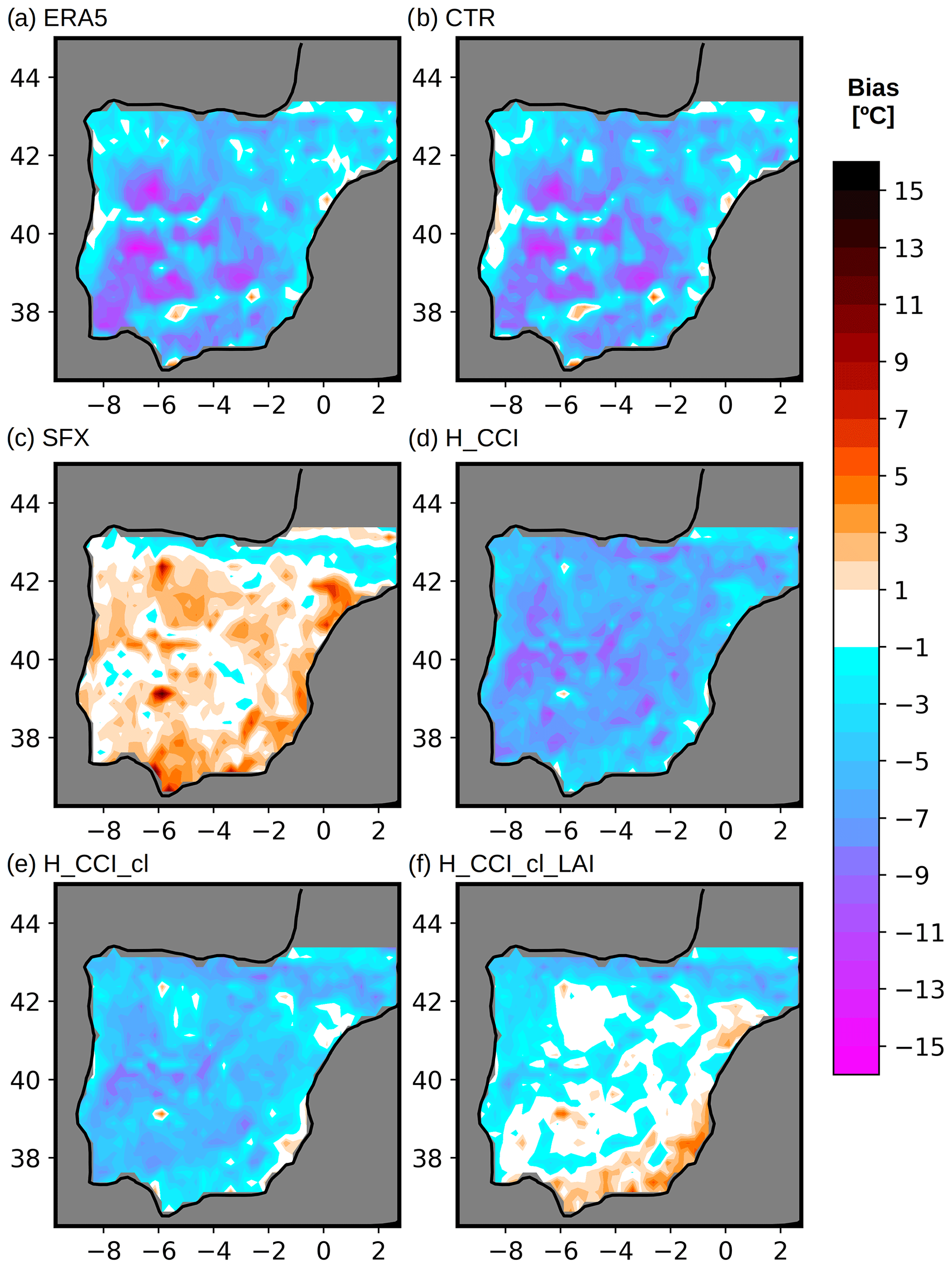
Figure 1Maps of JJA daily maximum LST bias over Iberia under clear-sky conditions, computed for different simulations. (a) ERA5; (b) CHTESSEL offline (CTR); (c) SURFEX offline (SFX); (d) H_CCI; (e) H_CCI_cl; and (f) H_CCI_cl_LAI. LSA-SAF LST was considered as reference for computing the simulation errors.
In addition to CTR and SFX, three additional simulations were performed with CHTESSEL, representing three different levels of updated vegetation coverage compared to CTR (see Table 1 for a summarized description of the main characteristics of the simulations considered in the present investigation). These additional simulations were carried over the same domain and period.
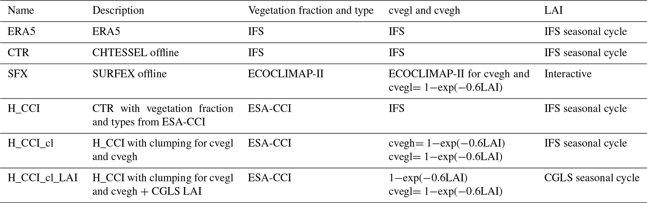
The first revised simulation, denoted H_CCI, focused on the vegetation fractions and types. In this revision, the high- and low-vegetation fractions and types were replaced in all grid points over Iberia by the data derived from the ESA-CCI land cover dataset. The original 300 m ESA-CCI land cover classes were spatially aggregated to the regular grid, generating fields with the fraction of each of the ESA-CCI 22 land cover class. These fractions were computed by counting the number of 300 m pixels of each class occurring within each of the grid cells. These fractional classes were then converted to the CHTESSEL land cover classes using a cross-walking table adapted from Poulter et al. (2015). These new land cover fractions were then processed to compute the fractional cover of low and high vegetation (CVl, CVh) and the dominant types of low and high vegetation attributed to each grid point. The vegetation density parameters (and other parameters associated with each dominant vegetation type) were obtained from the CHTESSEL lookup tables (see Table S1), analogous to the procedure in CTR, but taking the updated vegetation types and cover into account. The maps of CVl and CVh of CTR and H_CCI are shown in Supplement Fig. S1, along with a comparison between the dominant low- and high-vegetation types in CTR and H_CCI.
The two other simulations, denoted H_CCI_cl and H_CCI_cl_LAI, used the same updated vegetation based on ESA-CCI as H_CCI, but the low and high vegetation density parameters were revised. Following Alessandri et al. (2017), we employed clumping for high and low vegetation in both simulations, by introducing a Lambert–Beer law exponential dependence on LAI for both cvegl and cvegh as follows:
Equation (3) introduces a representation of the seasonal cycle for the high- and low-vegetation coverage. Notice that the vegetation clumping employed here is similar to the computation of cvegl in SURFEX (Le Moigne, 2018). However, in SURFEX cvegh was obtained from lookup tables based on vegetation cover types. In a preliminary analysis we tested the clumping for high and low vegetation or only for low vegetation in CHTESSEL. The results showed better performance of LST simulation when clumping was introduced for both high and low vegetation. Here a value of was considered for Eq. (3), which is the same value used in SURFEX for cvegl. Alessandri et al. (2017) used , but the impact of using 0.5 or 0.6 in the LST simulation was small.
The difference between H_CCI_cl and H_CCI_cl_LAI simulations was in the LAI fields provided as input to CHTESSEL. Notice that in all CHTESSEL simulations, LAI was prescribed as a mean monthly climatology for each grid point. Simulation H_CCI_cl used the original LAI fields in CHTESSEL (as in CTR and H_CCI). But H_CCI_cl_LAI used the LAI fields from the CGLS database. For this purpose, the 10-daily version 2 CGLS LAI was processed for the period 1999–2018 to generate the mean monthly climatology computing the monthly mean for each calendar month in the full 20-year period. This generated a climatology at 1 km that was then aggregated to the regular resolution by mapping the 1 km grid into the coarser grid. The motivation for updating the LAI fields in H_CCI_cl_LAI was provided by the high sensitivity of maximum daily LST on the vegetation density parameters reported by JO19. Consequently, Eq. (3) should introduce a significant sensitivity of daily maximum LST on LAI.
3.2 Simulation evaluation metrics
An overall evaluation of the clear-sky skin temperature estimates derived from the considered model-based datasets is shown in Table 2, using the LSA-SAF LST product as reference. Restricting the analysis to summer months (June–July–August, JJA) maximized the sampling for both model and satellite LST values, since cloud coverage remains relatively low in Iberia during summer months, as shown by JO19. We notice that, although the sample of LSA-SAF LST estimates was reduced outside the summer months due to cloud cover, it was still possible to perform a comparison of the seasonal cycle of daytime maximum and nighttime minimum LST using the available clear-sky data points amongst the different datasets considered in the present investigation. This comparison provides a quantitative measure of the impact of the use of different land surface models and different vegetation coverage formulations throughout the seasonal cycle.
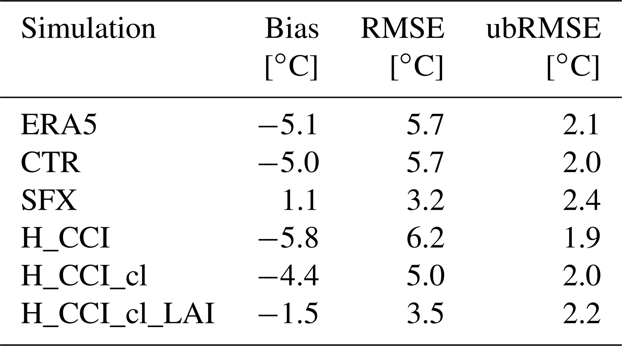
Table 2Bias, RMSE, and ubRMSE (unbiased RMSE) computed from JJA daily maximum LST bias average over entire Iberia, for each model-based dataset considered in the present study, using LSA-SAF LST as reference.
For the comparison between simulated and observed LST to be consistent, we performed an upscaling of the LSA-SAF LST hourly data, by computing the median of the whole group of LSA-SAF LST pixels (at 3 km resolution) inside each grid cell. The spatial aggregation using the mean was also tested, and the differences, when compared with the median, were negligible. The fraction of valid pixels (each grid cell and time) was retained during the upscaling procedure and used as a proxy to compute clear-sky fraction. Subsequently, for each grid cell over Iberia, only the instances where the percentage of valid LSA-SAF pixels was greater than 70 % and the ERA5 total cloud cover was below 30 % were considered for dataset comparison. These two thresholds were chosen based on JO19, corresponding to a balance between ensuring most of the grid cell to be cloud-free while keeping a large amount of valid data for the JJA 2004–2015 period over Iberia.
The daily maximum LST (LSTmax) was computed as the maximum value over the 11:00 to 18:00 UTC interval, while daily minimum LST (LSTmin) was computed as the minimum over the 00:00 to 07:00 UTC interval. These ranges were chosen to avoid the identification of daily extremes during time periods which are not representative of the minimum nocturnal and maximum afternoon temperature (for example, under cloudy daytime and clear-sky nighttime conditions, one would identify LSTmax during the latter).
Additionally, we estimated the maximum monthly FCOVER over Iberia in the different simulations considered here and compared against the CGLS FCOVER. Here the assumption was that the maximum monthly FCOVER derived from the satellite corresponds to 1 minus the permanent bare soil coverage. In turn, the percentage of bare soil may be estimated from land surface models from by employing Eq. (2). We also compared the fractions of low and high vegetation (i.e., Cl and Ch, respectively) amongst the different simulations. When analyzing these comparisons amongst the vegetation coverage in the different simulations, it is important to keep in mind that the CGLS FCOVER is tightly related to the CGLS LAI (they are derived from the same observations), which is given as input for H_CCI_cl_LAI. Additionally, the ESA-CCI vegetation cover is also used in constructing the ECOCLIMAP-II used by SURFEX. Nonetheless, these comparisons provided relevant insights into the differences in the LST fields amongst the different simulations as discussed below.
Finally, we also compared the surface evaporation from the different simulations considered here and from the GLEAMv3b dataset over the different seasons. Surface evaporation estimates from GLEAMv3b have non-negligible uncertainties. In this sense it should be regarded as an additional product against which the also-uncertain simulated evaporation pattern can be compared, rather than the truth. Nonetheless, this multi-dataset comparison provided a quantitative measure into the potential impact of the changes in vegetation cover and LST to the surface water and energy balances over Iberia.
4.1 Evaluation of summer daily maximum LST over Iberia
The daily maximum LST from ERA5 displayed a large cold bias over Iberia during JJA (JO19 and Fig. 1a), with magnitudes larger than 10 ∘C over wide portions of central and southwestern Iberia. Fig. 1b shows that the spatial pattern of daily maximum LST bias over Iberia in ERA5 was very closely reproduced by the control CHTESSEL offline simulation (CTR). This result opened a path to investigate, attempt to understand, and correct the summer daily maximum LST error sources over Iberia focusing on limited area CHTESSEL offline simulations, rather than running the full global coupled IFS model.
The spatial pattern of JJA daily maximum LST bias over Iberia simulated by SURFEX (SFX; Fig. 1c) was clearly distinct from CTR. Overall SFX displayed a smaller magnitude and positive bias over most of Iberia, except for the northernmost regions. The lower magnitude of the JJA LSTmax over Iberia in SFX compared to CTR and ERA5 was further evidenced by comparing the JJA daily max LST RMSE maps (Fig. 2a–c). The RMSE averaged over all Iberia grid points was 3.2 ∘C in SFX, well below the 5.7 ∘C value found for ERA5 and CTR. Similarly, the JJA LSTmax bias averaged over all Iberia grid points was 1.1 ∘C in SFX but −5.1 ∘C in ERA5 and −5.0 ∘C in CTR (see Table 2 for a summary of the overall errors in all the considered simulations). Notice that the bias and RMSE patterns in Figs. 1 and 2 were closely related. The RMSE was used here to provide a better visualization of the reduction in the systematic error magnitude between different simulations, since the differences in unbiased RMSE amongst all simulations were within the observational uncertainty associated with LSA-SAF LST (cf. Supplement Fig. S2). The large differences in the LSTmax errors between ERA5/CTR and those of SFX suggest that the errors in CTR were not due to the atmospheric forcing since SFX was driven by the same data. Moreover, the spatial patterns of RMSE were also nearly identical between ERA5 and CTR, providing further support to the use of offline CHTESSEL simulations to investigate the causes of the LST systematic errors in ERA5 over Iberia during JJA.
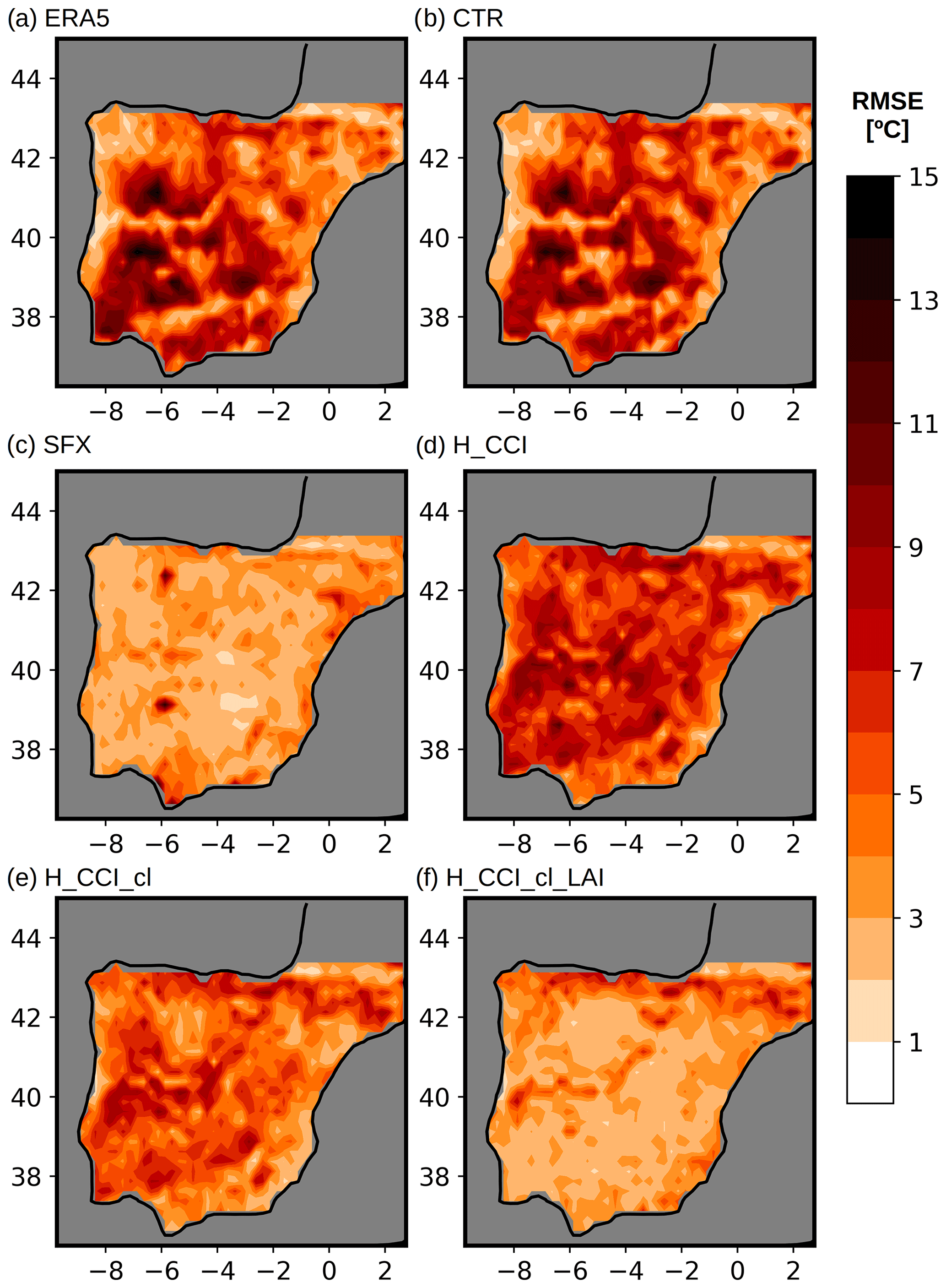
Figure 2Same as Fig. 1 but for RMSE.
4.2 Relation between the Iberia LST bias and the vegetation cover
Figure 3 shows scatterplots of JJA LSTmax bias versus the maximum monthly FCOVER error over Iberia. The latter was estimated from absolute differences between model and CGLS fractions of green vegetation cover. The results showed a relation between the LSTmax bias and the absolute error in maximum FCOVER in ERA5 (Fig. 3a) and CTR (Fig. 3b), with correlation coefficients of −0.4 and −0.5, respectively, and with largest LSTmax bias occurring for large FCOVER absolute errors. Furthermore, we found that, in general, the maximum monthly FCOVER in ERA5 and CTR (Fig. 4b) largely overestimated the CGLS FCOVER (Fig. 4a) over most of the regions of Iberia where large daily maximum LST bias (cf. Fig. 1) and RMSE (cf. Fig. 2) values were found for these datasets. We point out that the vegetation cover fields are identical in ERA5 and CTR. In contrast, SFX displayed lower values for both LST bias and absolute maximum monthly FCOVER error, with a correlation coefficient of only 0.2 between these two errors (Fig. 3d). Furthermore, the maximum FCOVER pattern estimated from SFX (Fig. 4c) was closer to the CGLS dataset, although SFX also tends to overestimate the FCOVER. Overall, these results support the hypothesis that at least part of the error in daily maximum LST during summer over Iberia in CHTESSEL (and thus in ECMWF products) was due to its misrepresentation of the vegetation coverage in this region. This hypothesis was also recently put forward in JO19, which reported a similar relation between the summer LST bias and the misrepresentation of summer FCOVER over Iberia. In the same sense, the significantly improved representation of the vegetation coverage over Iberia in SURFEX (largely due to its use of the ECOCLIMAP-II database) corresponds to a drastic reduction in the summer LST errors over Iberia.
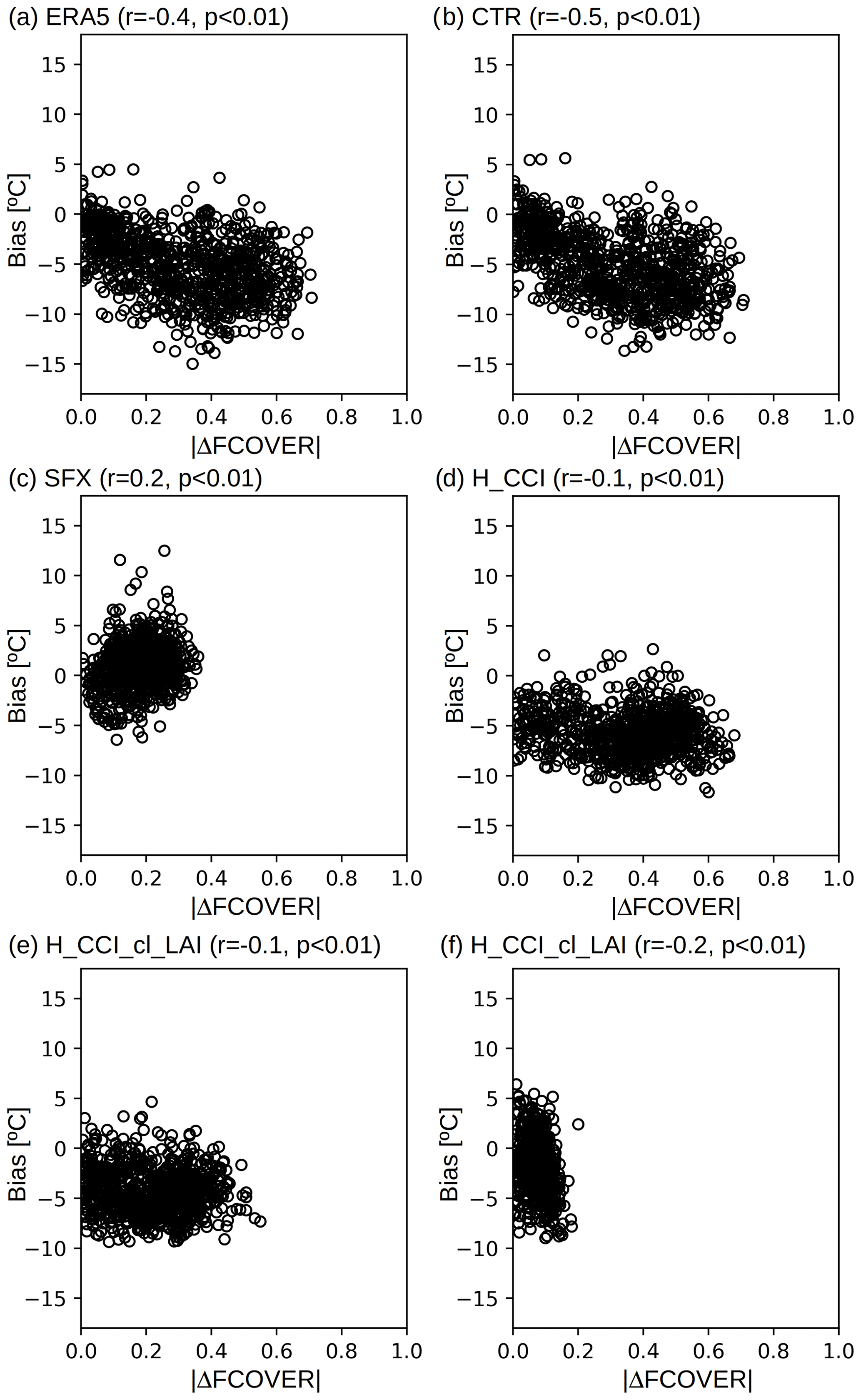
Figure 3Scatterplots of grid point JJA LSTmax bias over Iberia under clear-sky conditions against absolute error in monthly maximum FCOVER. (a) ERA5; (b) CTR; (c) SFX; (d) H_CCI; (e) H_CCI_cl; and (f) H_CCI_cl_LAI. LSA-SAF LST was considered as reference for computing the LSTmax errors, while CGLS FCOVER was considered as reference for computing the FCOVER errors. The Pearson correlation coefficient (r) and respective p value are shown for each simulation.
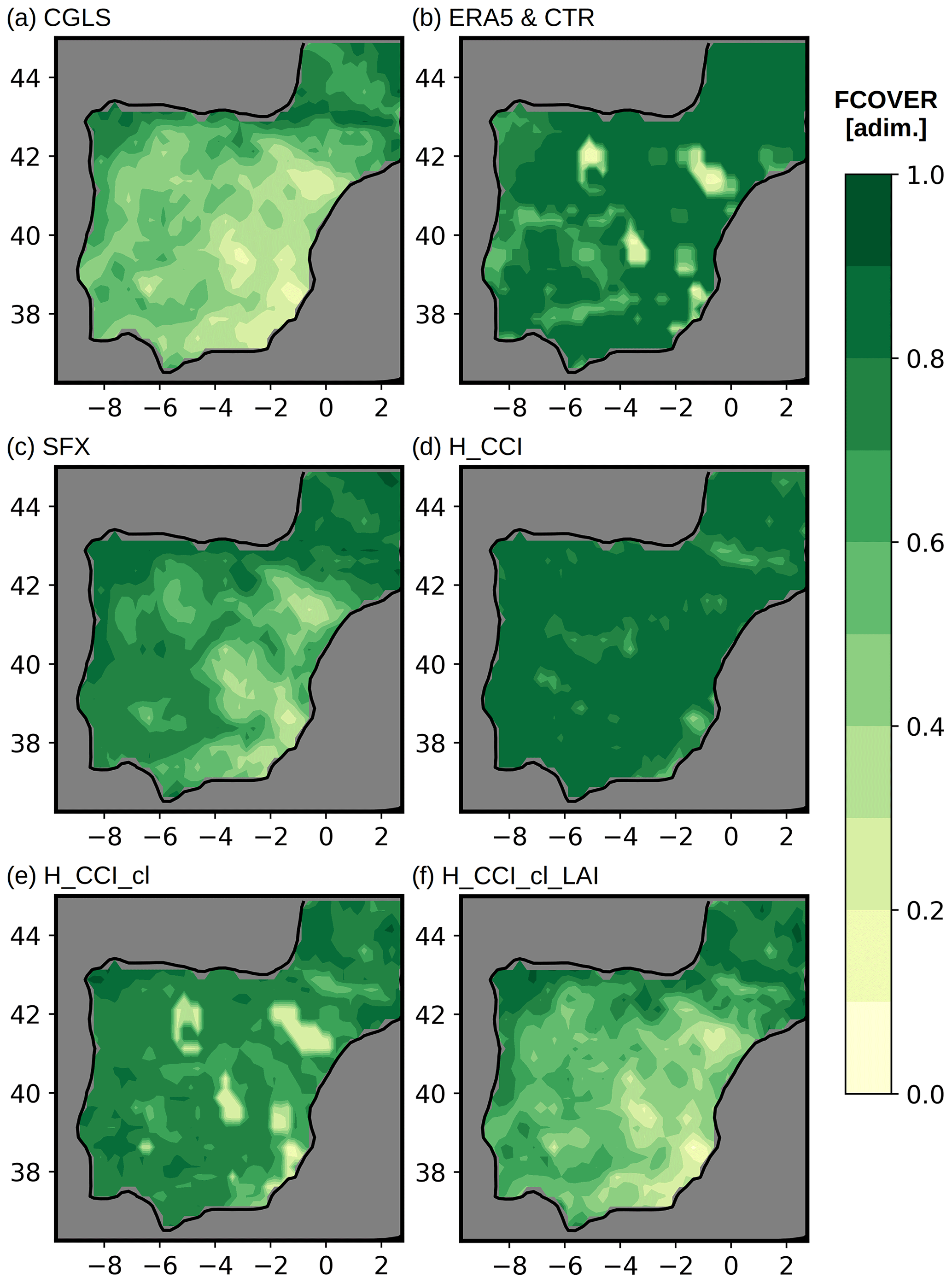
Figure 4Fraction of green vegetation coverage (FCOVER) from (a) CGLS dataset, (b) ERA5 and CTR (the FCOVER is identical for these two datasets), (c) SFX, (d) H_CCI, (e) H_CCI_cl, and (f) H_CCI_cl_LAI.
Subsequently, we compared the fractions of high and low vegetation (i.e., Ch and Cl) between the original CHTESSEL-based products (ERA5 and CTR) and SFX during JJA. On the one hand, the Cl over wide portions of Iberia was larger in the original CHTESSEL-based products (Fig. 5a, particularly in the north) than in SFX (Fig. 5c). On the other hand, ERA5 and CTR displayed significantly larger Ch values (Fig. 5b) compared to SFX (Fig. 5d) throughout most of Iberia, except for the northwestern region where the reverse is true. We notice that many of the regions with largest differences in Ch between CHTESSEL and SURFEX correspond to regions with the largest cold bias in summer daily maximum LST (cf. Fig. 1) and largest magnitude of RMSE (cf. Fig. 2) in ERA5 and CTR. Thus, we propose that the misrepresentation of the high- and low-vegetation coverages in CHTESSEL is a key source for the systematic cold bias found for the simulated summer daily maximum LST over Iberia.
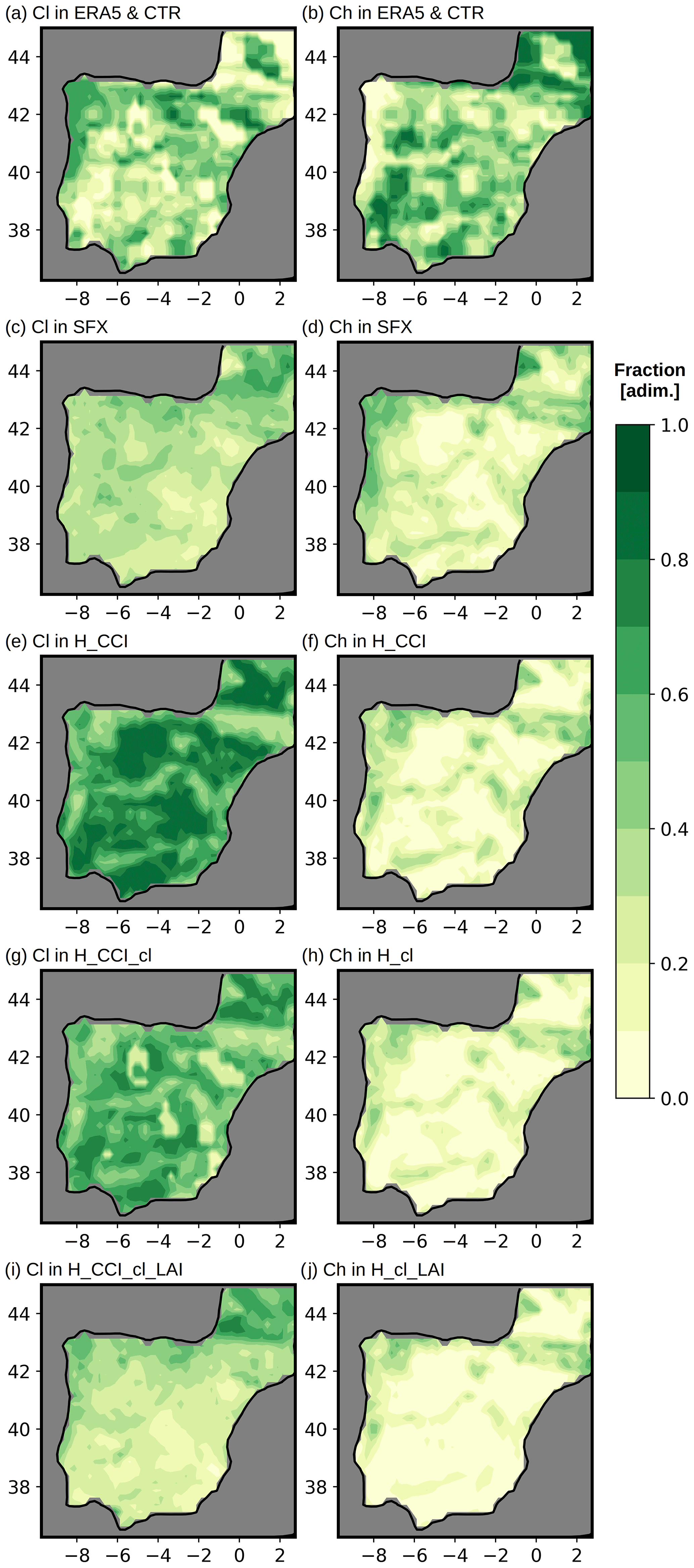
Figure 5Fraction of low-vegetation (Cl; left column) and high-vegetation (Ch; right column) coverage averaged over JJA. From top to bottom, the panels represent Cl and Ch in CTR (which is identical to ERA5), SFX, H_CCI, H_CCI_cl, and H_CCI_cl_LAI.
5.1 Impact of updated vegetation on JJA daily maximum LST
The results presented in Sect. 4 highlight the large cold bias affecting summer daily maximum LST over Iberia in the ECMWF products. In contrast, given the same atmospheric forcing, SURFEX displayed a lower-magnitude – and positive – LST bias. One of the key differences between the two models was the representation of vegetation coverage over Iberia. In this section, we evaluate the impact of the changes in vegetation coverage in the LST simulations. First, in simulation H_CCI the high- and low-vegetation fractions and types were modified based on the ESA-CCI database. Compared to CTR, H_CCI did not show a consistent reduction in summer daily maximum LST bias (Fig. 1d) nor RMSE (Fig. 2d) throughout most of Iberia. This was also illustrated by the bias and RMSE boxplots computed from CTR and H_CCI in Fig. 6. Although the largest-magnitude errors and overall error spread were reduced in H_CCI, the median increased slightly compared to CTR. Averaged over Iberia, the overall bias increased from −5.0 to −5.8 ∘C and the overall RMSE increased from 5.7 to 6.2 ∘C (see Table 2). The reason for the poor performance of H_CCI may be understood by analyzing its vegetation cover. Although H_CCI displayed a reduced correlation between LST bias and maximum monthly FCOVER absolute error (; Fig. 3d), it also displayed an overall larger overestimation of the maximum monthly FCOVER (Fig. 4d) when compared to CTR (Fig. 4b). The cause for this increased FCOVER was the widespread overestimation of the fraction of low vegetation (Fig. 5e), despite the fraction of high vegetation being significantly closer to SFX (Fig. 5f) (ECOCLIMAP-II was assumed here to have a more realistic vegetation coverage than the original CHTESSEL formulation).
The large overestimation of the fraction of low vegetation in H_CCI was due to an overestimation of the low vegetation density parameter, cvegl. This is a critical parameter in determining the amplitude of the diurnal cycle of LST over Iberia during summer months, as shown by JO19. In the original CHTESSEL formulation, the vegetation density parameters were obtained from lookup tables, based on the dominant vegetation types for each grid box. With the clumping parameterization introduced in H_CCI_cl, the vegetation density parameters were estimated as a function of the LAI, following Eq. (3), while considering the default LAI data used in the CTR. This resulted in a moderate reduction in the summer fraction of low vegetation (Cl; Fig. 5g) compared to CTR and to H_CCI, while the fraction of high vegetation remained nearly identical to H_CCI (Ch; Fig. 5h). Consequently, the Cl reduction leads to a moderate reduction in the maximum monthly FCOVER in H_CCI_cl (Fig. 4e) compared to CTR (Fig. 4b) and to H_CCI (Fig. 4d). As expected, the increased amount of bare soil (by reducing the vegetation coverage) leads to enhanced daytime warming, thus reducing the magnitude of the cold LSTmax bias over most of Iberia (Fig. 1f) and, consequently, also reducing the RMSE (Fig. 2f). The overall summer LSTmax bias averaged over Iberia was −4.4 ∘C in H_CCI_cl, −5.0 ∘C in CTR, and −5.8 ∘C in H_CCI (Table 2). The overall RMSE reduced from 5.7 ∘C in CTR (and 6.2 ∘C in H_CCI) to 5.0 ∘C in H_CCI_cl. The bias and RMSE boxplots in Fig. 6 also illustrate this reduction, although they also evidence that the errors in summer LSTmax in SFX were lower than in H_CCI_cl.
The maximum monthly FCOVER from H_CCI_cl (Fig. 4e) still represents an overestimation of the CGLS dataset (Fig. 4a), although slightly improved compared to CTR (Fig. 4b) and H_CCI (Fig. 4d). The pattern of summer fraction of high vegetation in H_CCI_cl (Fig. 5h) was similar to H_CCI (Fig. 5f) and SFX (Fig. 5d). However, the large overestimation of the summer fraction of low vegetation in H_CCI (Fig. 5e) was only moderately decreased in H_CCI_cl (Fig. 5g) and still larger than the values found in SFX over most of Iberia (Fig. 5c). Updating the vegetation fractions and types based on ESA-CCI resulted in major changes in the areas dominated by high and low vegetation between CTR and H_CCI or H_CCI_cl (Fig. 4). However, the LAI field used in H_CCI_cl to compute the vegetation density parameters was not updated and corresponds to the original vegetation distributions in CTR. We argue that this can generate some inconsistencies and limits the potential improvement in the representation of summer LST in H_CCI_cl. Consequently, a third simulation was introduced (denoted H_CCI_cl_LAI), which included the revised vegetation fractions and types based on ESA-CCI, the clumping parameterization, and updated LAI fields from CGLS database. Figure 5 shows that the summer fractions of high vegetation in H_CCI_cl_LAI were also similar to CTR, H_CCI, and H_CCI_cl. However, it also shows that the summer fraction of low vegetation was significantly reduced in H_CCI_cl_LAI compared to the other CHTESSEL simulations, rendering its pattern much closer to SFX.
The maximum monthly FCOVER was also reduced in H_CCI_cl_LAI over wide portions of Iberia, resulting in a closer match to the CGLS FCOVER compared to the previous CHTESSEL simulations (Fig. 4). This match in FCOVER between H_CCI_cl_LAI and CGLS was not surprising since the CGLS LAI and the CGLS FCOVER are tightly related to each other. A better, more independent way, to evaluate the impact of the revised vegetation cover is to analyze the simulated summer LSTmax fields. The results showed that the overall bias averaged over Iberia was −1.5 ∘C for H_CCI_cl_LAI (Table 2). This was much lower than the values of −4.4 ∘C in H_CCI_cl and −5.0 ∘C for CTR and closer in magnitude to the 1.1 ∘C found for SFX. Similarly, the overall RMSE was 3.5 ∘C for H_CCI_cl_LAI, 5.0 ∘C in H_CCI_cl, 3.2 ∘C in SFX, and 5.7 ∘C in CTR. The boxplots of summer daily maximum LST bias and RMSE over Iberia confirm the large error reduction in H_CCI_cl_LAI compared to all other CHTESSEL simulations, with the overall performance becoming very close to SFX. This is also illustrated by comparing the spatial patterns of bias and RMSE in Figs. 1 and 2, respectively. Finally, it should be noted that LST bias and RMSE patterns attained by SFX and H_CCI_cl_LAI were already very close to the accuracy values generally attributed to satellite LST values (Trigo et al., 2011; Göttsche et al., 2016).
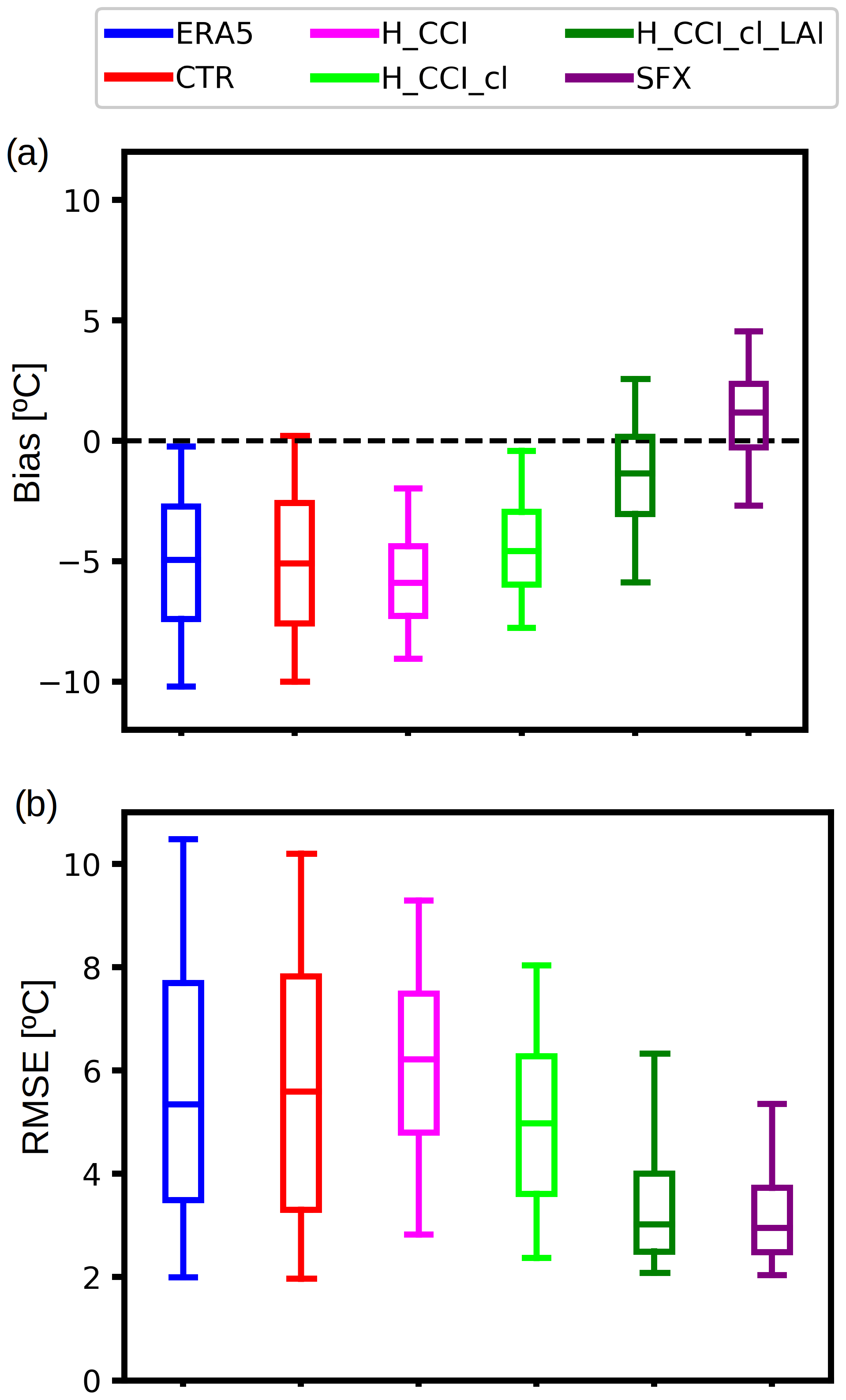
Figure 6Boxplots of JJA daily maximum (a) LST bias and (b) RMSE computed over the 2004–2015 period for from ERA5 (blue), CTR (red), H_CCI (pink), H_CCI_cl (light green), H_CCI_cl_LAI (dark green), and SFX (purple). The boxplot spread represents different grid points over Iberia. Only time instants under clear-sky conditions are considered. The boxes represent the 25th-to-75th percentiles, while the whiskers represent the 5th and 95th percentiles.

Figure 7Diurnal cycles of JJA (a) LST, (b) latent heat flux, and (c) sensible heat flux averaged over all Iberia grid points, computed from LSA-SAF (black), ERA5 (blue), SFX (purple), CTR (red), H_CCI (pink), H_CCI_cl (light green), and H_CCI_cl_LAI (dark green). Only time instants under clear-sky conditions were considered.
We compared the full diurnal cycle of the summer LST in all datasets considered here, in order to assess the differences in the Iberia summer LST amongst datasets outside of the time of daytime maximum. Figure 7 shows the JJA LST at each hour of the day averaged over the 2004–2015 period and over all Iberia grid points (only considering clear-sky conditions in both satellite and simulations). The average warming rate during the morning in LSA-SAF was overestimated in SFX, resulting in a slight warm bias of LSTmax, but underestimated by CHTESSEL, resulting in the cold bias found for CTR and ERA5. H_CCI displayed a slightly larger underestimation of the morning warming rate compared to CTR, thus increasing the magnitude of the cold bias. H_CCI_cl showed only a slight increase in the morning warming rate compared to CTR but was still well below the LSA-SAF warming rate. In H_CCI_cl_LAI the morning warming rate was much closer to LSA-SAF, resulting in larger reduction in the LSTmax cold bias, of similar magnitude to the warm bias in SFX. During the afternoon the cooling rate tends to be slightly slower in all models than in observations, but the resulting differences in nighttime LST are relatively small amongst all datasets (below 2 ∘C) and, thus, within the typical uncertainty associated with the LSA-SAF LST estimates of around 1–2 K over Iberia (Trigo et al., 2011).
One must notice the slight shift of the time of maximum LST in all simulations using CHTESSEL (ERA5, CTR, H_CCI, H_CCI_cl, and H_CCI_cl_LAI) to 14:00 UTC, 1 h later than for LSA-SAF. We point out that SFX did not display this phase shift, peaking at 13:00 UTC. The latent heat fluxes (Fig. 7b) also displayed a noticeable shift between SFX and CHTESSEL-based simulations, but no reliable subdaily observations were available to provide a baseline for this comparison. JO19 identified a large shift in the diurnal cycle of simulated LST simulations when using 1 h time step in offline CHTESSEL simulations. This was partially mitigated with the reduction in the time step to 15 min (as used in this study). Also in that study, the increased vertical resolution in the soil (changing the top layer from 7 to 1 cm) had a positive impact on the diurnal cycle shift. Therefore, this shift was mainly attributed to the numerics of the model, and further attention is required, looking at the time step (implicit coupling between skin energy balance solver and soil vertical diffusion), vertical discretization of the soil, and coupling between skin layer and underlying soil. However, such detailed investigation of this issue is beyond the scope of this study. Nonetheless, despite the noticeable time lag, the diurnal cycle in Fig. 7a revealed that the SFX and H_CCI_cl_LAI correspond to a much better representation of the observed diurnal cycle amplitude compared to ERA5 and CTR.
5.2 Impact of updated vegetation on LST outside summer
The seasonal cycle of LSTmax averaged over Iberia during the 2004–2015 period from all datasets is shown Fig. 8a considering all-sky conditions and in Fig. 8b considering clear-sky conditions. The respective seasonal cycle of LSTmin under all-sky and clear-sky conditions are shown in Fig. 8c and Fig. 8d. The monthly mean LSTmax averaged over Iberia was identical between ERA5 and CTR throughout the entire year both under all-sky (Fig. 8a) and clear-sky conditions (Fig. 8b), providing further robustness to the use of the offline simulations to assess the systematic errors of LST over Iberia in ERA5 dataset and their main sources.
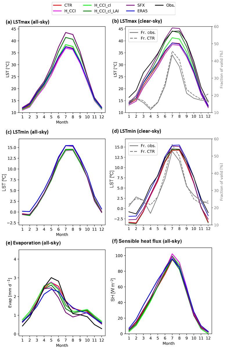
Figure 8Seasonal cycles of daily maximum LST (a) under all-sky and (b) clear-sky conditions; daily minimum LST under (c) all-sky and (d) clear-sky conditions; (e) daily total evaporation under all-sky conditions and (f) daily mean sensible heat flux under all-sky conditions. All panels represent averages taken over all Iberia grid points considering all-sky conditions, for each month during the 2004–2015 period. Observations are available for LST under clear-sky conditions (LSA-SAF, black lines in panels b and d) and for evaporation (GLEAM dataset, black line in panel c). The gray lines in panels (b) and (d) represent the fraction of valid data points used to compute the clear-sky averages for LSA-SAF (full line) and model simulations (dashed), with the scale given by the y axis on the righthand side.
The monthly-averaged LSTmax was generally warmer throughout the entire yearly cycle for clear-sky (Fig. 8b) conditions than for all-sky conditions (Fig. 8a). This was expected given the tight relation between LSTmax and downward solar radiation at the surface. The difference between clear- and all-sky conditions was largest during summer months for simulations using clumping (H_CCI_cl and H_CCI_cl_LAI) due to the increased bare soil in these cases. Nonetheless, similar conclusions may be derived for the seasonal cycle of LSTmax under both all-sky and clear-sky conditions. First and foremost, during colder months the differences amongst all simulations are below ∼1 ∘C and, thus, within observational uncertainty. This means that the differences in LSTmax between simulations outside the warm months were essentially neutral (within the LSA-SAF LST uncertainty), both considering all-sky and clear-sky conditions. Interestingly, Fig. 8b shows a systematic underestimation of simulated LSTmax during cold months compared to observations. However, this systematic error should be interpreted with care, since Fig. 8b also shows that the fraction of valid data points (out of all the available data points, including all pixels in Iberia and all days in the 2004–2015 period) reduces from ∼40 % during JJA to ∼20 % or less during December–January–February. On the other hand, during warm months (roughly April to September), where the fraction of clear-sky data points increases, we found large reductions in the LSTmax cold bias for simulations H_CCI_cl_LAI and SFX.
The seasonal cycle of LSTmin averaged over Iberia is shown in Fig. 8c considering all-sky conditions and in Fig. 8d considering clear-sky conditions. Both clear- and all-sky averages revealed that the differences amongst all the considered datasets (LSA-SAF, ERA5, CTR, H_CCI, H_CCI_cl, H_CCI_cl_LAI, and SFX) were all below 1.2 ∘C and, thus, within the LSA-SAF LST uncertainty. Overall, these results show that the systematic errors associated with LSTmin were lower than for LSTmax and that the updated vegetation coverage had little impact on the nighttime minimum temperature throughout the entire year, in agreement with the results of the JJA LSTmin diurnal cycle in Fig. 7.
Simulation H_CCI_cl_LAI features an updated representation of vegetation over Iberia compared to the original CHTESSEL formulation, namely with revised LAI and vegetation fractions and types, and a clumping parameterization for the vegetation density parameters. Compared to the CTR simulation, H_CCI_cl_LAI resulted in a closer agreement to the fractions of low and high vegetation during summer in SFX, derived from ECOCLIMAP-II. Additionally, it also resulted in a closer match to the maximum monthly FCOVER from the CGLS dataset. Both these comparisons must be interpreted with care. On the one hand, H_CCI_cl_LAI uses the CGLS LAI, which in turn is tightly related to the CGLS FCOVER. On the other hand, ECOCLIMAP-II uses information on the vegetation cover from the ESA-CCI dataset. Furthermore, SFX also uses a clumping parameterization for the low vegetation density parameter (but not for the high vegetation parameter).
Nonetheless, a robust support to the added value of the corrections implemented in H_CCI_cl_LAI was provided by comparing the simulated LST amongst datasets. Our results showed a large reduction in the summer daily maximum LST cold bias in H_CCI_cl_LAI when compared to CTR. Additionally, we found relatively small differences (within typical LSA-SAF LST observation uncertainty of 1–2 K; Göttsche et al., 2016) amongst these two datasets during winter and during nighttime. This suggests that the implemented changes were robust, in the sense that the simulated LST is improved during daytime in warm months, with negligible impacts in all other months and hours of the day. Furthermore, the fact that SFX displayed similar performance in the simulation of LST provided further support to the results of H_CCI_cl_LAI.
Interestingly, simulation H_CCI did not reduce the cold bias in summer daily maximum LST over Iberia, while H_CCI_cl resulted only in a slight reduction. These results highlight an important point: the revision of the vegetation coverage in the CHTESSEL model must be implemented consistently throughout its multiple dimensions. Updating the vegetation types and fractions based on ESA-CCI from the original CHTESSEL formulation resulted in an error reduction for the JJA LSTmax over the regions affected by the largest bias (Fig. 9b), which were dominated by high vegetation in the original CHTESSEL and became dominated by low vegetation in H_CCI. However, over the regions which were dominated by low vegetation in the original CHTESSEL formulation and became dominated by high vegetation in H_CCI, the RMSE increased (cf. Figs. 9b and 5). Sensitivity tests over these regions of increased error suggest that this was due to an overestimation of the low vegetation density parameters. Indeed, introducing clumping in H_CCI_cl slightly reduced the cvegl parameter over these regions, reducing the errors (Fig. 9c). However, the LAI used for the clumping parameterization in H_CCI_cl corresponded to the original CHTESSEL data, where the grid points dominated by low and high vegetation were essentially reversed when compared to ESA-CCI (Fig. 5). Thus, updating the LAI becomes necessary after updating the vegetation fractions and types and introducing clumping. Indeed, H_CCI_cl_LAI resulted in significantly larger error reduction over the regions of large cold bias and only very slight error increases (within observation uncertainty) over the regions where the updated model is dominated by high vegetation (Fig. 9d). Similarly, SFX, which features similar vegetation types and fractions, clumping for low vegetation and interactive LAI (thus coherent with its vegetation cover), resulted in much lower bias compared to CTR over regions dominated by low vegetation and similar bias over regions dominated by high vegetation (Fig. 9a).
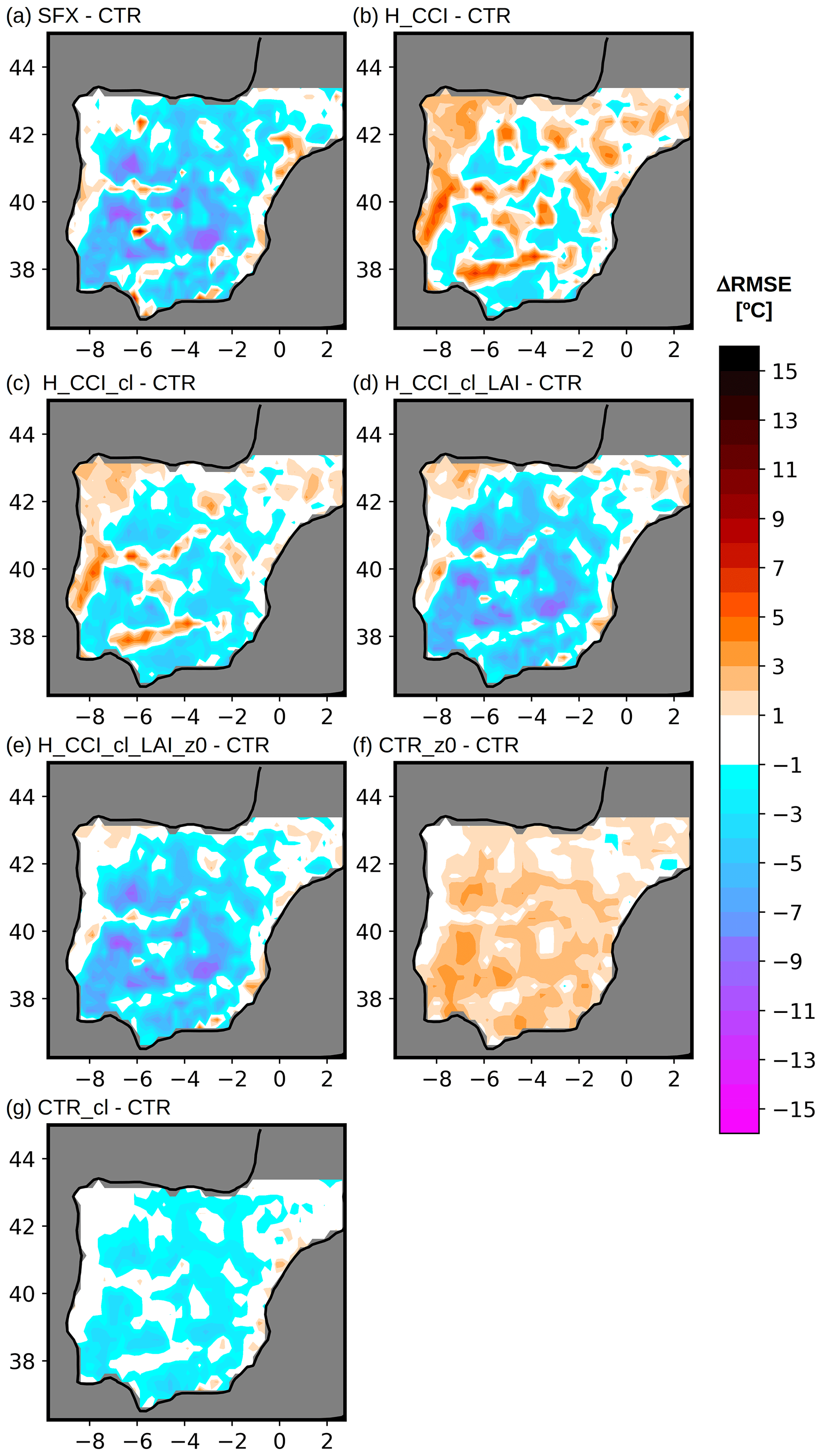
Figure 9Difference in RMSE computed for daily maximum LST over Iberia in (a) SFX minus CTR, (b) H_CCI minus CTR, (c) H_CCI_cl minus CTR, (d) H_CCI_cl_LAI minus CTR, (e) H_CCI_cl_LAI_z0 (same as H_CCI_cl_LAI but with z0h reduced by a factor of 10) minus CTR, (f) CTR_z0 (same as CTR but with z0h reduced by a factor of 10) minus CTR, and (g) CTR_cl (same as CTR but with clumping parameterization for high and low vegetation) minus CTR.
We point out that further improvement of the simulated surface temperature may be obtained by changing other relevant surface parameters. For example, we tested changing the surface roughness length for heat transfer, z0h, which plays an important role for the surface skin layer energy budget. We notice that in the original CHTESSEL formulation, z0h is equal to surface roughness length for momentum, z0m, only for high-vegetation-dominated regions, while for low-vegetation-dominated regions z0h is lower than z0m by a factor of 100 (see Supplement Table S1). Reducing the roughness length for heat transfer for high-vegetation types in simulation H_CCI_cl_LAI by a factor of 10 results in a further reduction in the daily maximum LST errors over the regions dominated by high vegetation, essentially removing all error increases compared to CTR (Fig. 9e). It is important to highlight that the roughness length change was not effective by itself in removing the JJA cold bias in daily maximum LST over Iberia, but it played a relevant role for this purpose when updated together with all other corrections in H_CCI_cl_LAI. Indeed, Fig. 9f shows that reducing the roughness length for heat transfer by a factor of 10 for high-vegetation types directly in simulation CTR resulted in an overall increase in the errors over most of Iberia (particularly over all regions that were dominated by high vegetation in CTR). Other surface parameters also play an important role in simulated surface temperature, such as albedo and emissivity, which are also related to the surface vegetation coverage in LSMs (e.g., Nogueira and Soares, 2019).
Further support to the relevance of a systematic and coherent update of all dimensions of the surface vegetation coverage was provided by introducing the clumping parameterization directly in CTR, without updating LAI nor the vegetation fractions and types. This resulted only in moderate error reduction throughout Iberia (Fig. 9g), representing a much lower improvement when compared to H_CCI_cl_LAI.
Finally, the evaluation of other relevant surface variables is critical. For example, the changes to the vegetation cover and LST between H_CCI_cl_LAI and CTR should have a relevant impact on the surface energy and water budgets. Thus, evaluating the simulated surface water variables and water and energy fluxes is required for a complete validation of the implemented changes. However, these fields are strongly dependent on the surface–atmospheric feedbacks, and its validation based on offline simulation alone is not complete. Furthermore, there are very few reliable observational datasets over Iberia for these variables with appropriate accuracy to perform an effective model validation. In order to illustrate this problem, we compared the surface evaporation amongst the simulation datasets and with GLEAMv3b (Fig. 8e). During August to February, ERA5 and all offline simulations displayed a similar magnitude overestimation of GLEAMv3b evaporation. Surprisingly, the best performing simulations in terms of summer LSTmax (i.e., SFX and H_CCI_cl_LAI) showed the largest differences from GLEAMv3b during March to July. These differences were associated with a reduction in evaporation compared to CTR (Fig. 7b). Interestingly, the reduction in evaporation in SFX and H_CCI_cl_LAI compared to GLEAMv3b occurred over northwestern Iberia, which was dominated by low vegetation in CTR but became dominated by high vegetation in these two simulations (Fig. S3 in the Supplement). However, we notice that the seasonal cycle of Iberia average surface evaporation showed large differences between ERA5 and offline CHTESSEL, particularly between March and July, where ERA5 showed lower evaporation than GLEAMv3b (Fig. 8e). Indeed, the differences between ERA5 and CTR (which were primarily due to the soil moisture land data assimilation increments in ERA5) were of the same order of magnitude as the differences between CTR and H_CCI_cl_LAI.
The seasonal cycles of daily average sensible heat flux (Fig. 8f) displayed relatively small differences amongst the different simulations, which were similar to the differences between ERA5 and CTR. The summer mean diurnal cycle of sensible heat flux points out that differences up to ∼50 W m−2 may exist between different simulations (Fig. 7c), particularly for H_CCI. But these differences were removed by including clumping and updating LAI. In fact, the JJA sensible heat flux diurnal cycle in SFX and H_CCI_LAI_cl was closer to ERA5 than CTR. Yet, it is important to state that a rigorous evaluation of the changes to the surface energy and water budget associated with the proposed changes to CHTESSEL vegetation is required, using coupled land–atmosphere simulations covering a domain where appropriate surface flux observations are available. This task will be the subject of a subsequent work.
We used the LSA-SAF satellite product to evaluate the summer LST over Iberia simulated by two LSMs – CHTESSEL and SURFEX – during the 2004–2015 period. Both LSMs were run offline, forced by the same atmospheric forcing fields obtained from the recently released ERA5 reanalysis.
The results show a large cold bias of the JJA LSTmax simulated by CHTESSEL, reaching magnitudes larger than 10 ∘C over wide portions of central and southwestern Iberia. This large cold bias was shown to be tightly linked to a misrepresentation of the Iberia vegetation cover in CHTESSEL, when compared against ESA-CCI land cover dataset, CGLS FCOVER and ECOCLIMAP-II dataset. We show that this misrepresentation includes not only significant differences between the areas dominated by high- and low-vegetation types but also the amount of bare soil and the fractions of green cover. This result agreed with recent investigations reporting a tight link between the misrepresentation of the vegetation coverage and the errors in LST simulated by different LSMs over different regions of the globe (Zheng et., 2012; Trigo et al., 2015; Gou et al., 2019; and JO19). Accordingly, the summer LSTmax over Iberia simulated by SURFEX displayed a much smaller magnitude (positive) bias, which was within the uncertainty associated with LSA-SAF LST. One of the key reasons for this difference was the fact that SURFEX uses the updated land cover dataset ECOCLIMAP-II, and it includes interactive vegetation evolution, with a clumping parameterization for the low vegetation density parameter.
We propose a methodology to improve the representation of vegetation over Iberia in CHTESSEL by combining information from the ESA-CCI land cover dataset with the CGLS LAI. The proposed improvement in vegetation included an update of the LAI data and high- and low-vegetation fractions and types, together with introducing a clumping parameterization for both high and low vegetation density. The clumping introduced seasonality to the vegetation coverage due to an exponential dependence on the LAI. We demonstrate that the proposed improved representation of vegetation has significant added value, removing the daily maximum LST summer cold bias completely while never reducing the accuracy over all seasons and hours of the day.
By analyzing different simulations with different degrees of changes to the vegetation coverage in CHTESSEL, we show that in order for the vegetation revision to be effective, it must be implemented consistently across its multiple dimensions. Specifically, we showed that updating the vegetation types and fractions without a coherent update to the vegetation density parameters results in a slight degradation of the simulated LST compared to the original CHTESSEL simulation. Additionally, revising the vegetation density parameters by introducing the clumping parameterization introduced a strong dependency of the vegetation fraction on the LAI, which had only moderate benefit if the LAI fields was not revised. It was the combination of these multiple coherent improvements that resulted in a large bias reduction, towards error magnitudes that are within values of the LSA-SAF LST uncertainty. We point out that the proposed revised vegetation in CHTESSEL reduced the errors in JJA LSTmax without degrading the simulated LST for other times of the day or for other months of the year (to within the typical uncertainty associated with LSA-SAF estimates).
Finally, we point out that in the present study the proposed formulation was only tested for the offline simulated LST. It is important to assess the results of the revised vegetation coverage in other components of the surface water and energy budgets. However, as shown here for evaporation, this requires coupled land–atmosphere simulations, which will be the subject of a subsequent investigation. Furthermore, it requires accurate validation datasets, which are not always available.
Nonetheless, the present work has important implications. First, LST plays a central role in the surface–atmosphere energy and water exchanges, and thus, its accurate representation in LSMs is crucial for accurate Earth system models. Second, CHTESSEL is the LSM employed by ECMWF in the production of their weather forecasts and reanalysis; hence systematic errors in CHTESSEL are expected to affect these products. Indeed, we showed that pattern of the summer daily maximum LST cold bias over Iberia in CHTESSEL is also present in the widely used ERA5 reanalysis, while JO19 showed that it was also present in the ECMWF previous generation reanalysis ERA-Interim. In fact, the extensive similarity in summer LSTmax error patterns between ERA5 and the offline CHTESSEL simulation provided support for using the offline setup employed here to assess and improve the simulation of LST. Yet, we point out the necessity for future evaluation of the proposed updates to the CHTESSEL vegetation in coupled land–atmosphere simulations, as well as its extension to the rest of the globe. Finally, our results provided further support to the important role played by vegetation in land–atmosphere exchanges. Specifically, we highlight the relevance of consistent vegetation cover and corresponding seasonality for LST simulated by CHTESSEL and SURFEX, and we point out that Earth observations may be used for constraining and improving weather and climate simulations.
The SURFEX modeling platform of Météo-France is open source, can be downloaded freely at http://www.umr-cnrm.fr/surfex/ (CNRM, 2016), and uses the CECILL-C license (a French equivalent to the L-GPL license; http://cecill.info/licences/Licence_CeCILL_V1.1-US.html; CEA-CNRS-Inria, 2013). It is updated at a relatively low frequency (every 3 to 6 months). If more frequent updates are needed – or if what is required is not in Open-SURFEX (DrHOOK, FA/LFI formats or GAUSSIAN grid) – you are invited to follow the procedure to get an SVN account and to access real-time modifications of the code (see the instructions in the first link). The developments presented in this study stem from SURFEX version 8.1.
The ECMWF land surface model configurations described here are based on the CHTESSEL model. The CHTESSEL source code is available subject to a license agreement with ECMWF. ECMWF member state weather services and their approved partners will be granted access. The CHTESSEL code without modules related to data assimilation is also available for educational and academic purposes as part of the OpenIFS project (https://software.ecmwf.int/wiki/display/OIFS/OpenIFS+Home, last access: 31 August 2020, and https://confluence.ecmwf.int/display/OIFS/Offline+Surface+Model+User+Guide, last access: 31 August 2020). Further details regarding data availability and model configurations, including the information required to reproduce the presented results on ECMWF systems, are available from the authors on request.
ERA5 data can be obtained freely from the Copernicus Climate Change Service Information website (https://climate.copernicus.eu/, Copernicus Climate Change Service (C3S), 2019).
The CGLS FCOVER and LAI can be obtained freely from the CGLS website (https://land.copernicus.eu/, last access: 31 August 2020).
The ESA-CCI land cover can be obtained freely from their website (https://www.esa-landcover-cci.org/, last access: 31 August 2020).
The LSA-SAF LST can be obtained freely from their website (https://landsaf.ipma.pt/, last access: 31 August 2020).
All the considered fields (LST, evaporation, LAI, FCOVER, Ch, and Cl) from all the considered simulations considered in the present study as well as the source code of SURFEX-ISBA model are freely available at https://doi.org/10.5281/zenodo.3701230 (Nogueira et al., 2020). Due to license restrictions, the source of CHTESSEL cannot be made available publicly.
The supplement related to this article is available online at: https://doi.org/10.5194/gmd-13-3975-2020-supplement.
Conceptualization was done by MN and ED; numerical simulations and model development were done by ED, MN, CA, and SB; data acquisition and processing were done by FJ, SE, JPM, ED, and MN; formal analysis was done by MN; funding acquisition was done by ED; all authors contributed to writing, reviewing,and editing the paper
The authors declare no conflict of interest. The funders had no role in the design of the study; in the collection, analyses, or interpretation of data; in the writing of the manuscript or in the decision to publish the results.
This research was funded by Fundação para a Ciência e a Tecnologia (FCT) grant number PTDC/CTA-MET/28946/2017 (CONTROL). Emanuel Dutra was funded by FCT research grant IF/00817/2015. The authors would also like to acknowledge the financial support of FCT through project UIDB/50019/2020 – IDL. Acknowledgment is made for the use of ECMWF's computing and archive facilities in this research.
This research was funded by Fundação para a Ciência e a Tecnologia (FCT) under project CONTROL (grant number PTDC/CTA-MET/28946/2017) and also by grant UIDB/50019/2020 – IDL. Emanuel Dutra was funded by FCT research grant IF/00817/2015.
This paper was edited by Jatin Kala and reviewed by three anonymous referees.
Aires, F., Prigent, C., Rossow, W. B., and Rothstein, M.: A new neural network approach including first-guess for retrieval of atmospheric water vapor, cloud liquid water path, surface temperature and emissivities over land from satellite microwave observations, J. Geophys. Res., 106, 887–907, 2001.
Albergel, C., Dutra, E., Bonan, B., Zheng, Y., Munier, S., Balsamo, G., Rosnay, P. D., Sabater, J. M., and Calvet, J.: Monitoring and Forecasting the Impact of the 2018 Summer Heatwave on Vegetation, Remote Sensing, 11, 520, https://doi.org/10.3390/rs11050520, 2019.
Alessandri, A., Catalano, F., De Felice, M., Van Den Hurk, B., Doblas Reyes, F., Boussetta, S., Balsamo, G., and Miller, P. A.: Multi-scale enhancement of climate prediction over land by increasing the model sensitivity to vegetation variability in EC-Earth, Clim. Dynam., 49, 1215–1237, 2017.
Balsamo, G., Viterbo, P., Beljaars, A., van den Hurk, B., Hirschi, M., Betts, A. K., and Scipal, K.: A Revised Hydrology for the ECMWF Model: Verification from Field Site to Terrestrial Water Storage and Impact in the Integrated Forecast System, J. Hydrometeorol., 10, 623–643, 2009.
Bauer, P., Thorpe, A., and Brunet, G.: The quiet revolution of numerical weather prediction, Nature 525, 47–55, https://doi.org/10.1038/nature14956, 2015.
Beck, H. E., Pan, M., Roy, T., Weedon, G. P., Pappenberger, F., van Dijk, A. I. J. M., Huffman, G. J., Adler, R. F., and Wood, E. F.: Daily evaluation of 26 precipitation datasets using Stage-IV gauge-radar data for the CONUS, Hydrol. Earth Syst. Sci., 23, 207–224, https://doi.org/10.5194/hess-23-207-2019, 2019.
Belmonte Rivas, M. and Stoffelen, A.: Characterizing ERA-Interim and ERA5 surface wind biases using ASCAT, Ocean Sci., 15, 831–852, https://doi.org/10.5194/os-15-831-2019, 2019.
Best, M. J., Abramowitz, G., Johnson, H. R., Pitman, A. J., Balsamo, G., Boone, A. Cuntz, M., Decharme, B., Dirmeyer, P. A., Dong, J., Ek, M., Guo, Z., Haverd, V., van den Hurk, B. J., Nearing, G. S., Pak, B., Peters-Lidard, C., Santanello, J. A., Stevens, L., and Vuichard, N.: The Plumbing of Land Surface Models: Benchmarking Model Performance, J. Hydrometeorol., 16, 1425–1442, https://doi.org/10.1175/JHM-D-14-0158.1, 2015.
Bojinski, S., Verstraete, M., Peterson, T. C., Richter, C., Simmons, A., and Zemp, M.: The Concept of Essential Climate Variables in Support of Climate Research, Applications, and Policy, B. Am. Meteorol. Soc., 95, 1431–1443, https://doi.org/10.1175/BAMS-D-13-00047.1, 2014.
Boone, A. and Etchevers, P.: An Intercomparison of Three Snow Schemes of Varying Complexity Coupled to the Same Land Surface Model: Local-Scale Evaluation at an Alpine Site, J. Hydrometeorol., 2, 374–394, https://doi.org/10.1175/1525-7541(2001)002<0374:AIOTSS>2.0.CO;2, 2001.
Boussetta, S., Balsamo, G., Beljaars, A., Panareda, A.-A-, Calvet, J.-C., Jacobs, C., van den Hurk, B., Viterbo, P., Lafont, S., Dutra, E., Jarlan, L., Balzarolo, M., Papale, D., and van der Werf, G.: Natural land carbon dioxide exchanges in the ECMWF Integrated Forecasting System: Implementation and Offline validation, J. Geophys. Res., 118, 1–24, https://doi.org/10.1002/jgrd.50488, 2013.
Calvet, J.-C., Noilhan, J., Roujean, J.-L., Bessemoulin, P., Cabelguenne, M., Olioso, A., and Wigneron, J.-P.: An interactive vegetation SVAT model tested against data from six contrasting sites, Agr. Forest Meteorol., 92, 73–95, 1998.
Candy, B., Saunders, R. W., Ghent, D., and Bulgin, C. E.: the impact of satellite-derived land surface temperatures on numerical weather prediction analyses and forecasts, J. Geophys. Res.-Atmos., 122, 9783–9802, https://doi.org/10.1002/2016JD026417, 2017.
Copernicus Climate Change Service (C3S): ERA5: Fifth generation of ECMWF atmospheric reanalyses of the global climate, Copernicus Climate Change Service Climate Data Store (CDS), available at: https://cds.climate.copernicus.eu/ (last access: 15 June 2020), 2019.
Decharme, B., Brun, E., Boone, A., Delire, C., Le Moigne, P., and Morin, S.: Impacts of snow and organic soils parameterization on northern Eurasian soil temperature profiles simulated by the ISBA land surface model, The Cryosphere, 10, 853–877, https://doi.org/10.5194/tc-10-853-2016, 2016.
Dee, D. P., Uppala, S. M., Simmons, A. J., Berrisford, P., Poli, P., Kobayashi, S., Andrae, U., Balmaseda, M. A., Balsamo, G., Bauer, P., Bechtold, P., Beljaars, A.C.M., van de Berg, L., Bidlot, J., Bormann, N., Delsol, C., Dragani, R., Fuentes, M., Geer, A. J., Haimberger, L., Healy, S. B., Hersbach, H., Hólm, E. V., Isaksen, L., Kållberg, P., Köhler, M., Matricardi, M., McNally, A. P., Monge‐Sanz, B.M., Morcrette, J.-J., Park, B.-K., Peubey, C., de Rosnay, P., Tavolato, C., Thépaut, J.‐N., and Vitart, F.: The ERA‐Interim reanalysis: configuration and performance of the data assimilation system, Q. J. Roy. Meteor. Soc., 137, 553–597, https://doi.org/10.1002/qj.828, 2011.
Defourny, P., Boettcher, M., Bontemps, S., Kirches, G., Krueger, O., Lamarche, C., Lembrée, C., Radoux, J., and Verheggen, A.: Algorithm theoretical basis document for land cover climate change initiative, Technical report, European Space Agency, 2014.
de Rosnay, P., Drusch, M., Vasiljevic, D., Balsamo, G., Albergel, C., and Isaksen, L.: A simplified Extended Kalman Filter for the global operational soil moisture analysis at ECMWF, Q. J. Roy. Meteor. Soc., 139, 1199–1213, https://doi.org/10.1002/qj.2023, 2013.
Duan, S.-B., Li, Z.-L., and Leng, P.: A framework for the retrieval of all-weather land surface temperature at a high spatial resolution from polar-orbiting thermal infrared and passive microwave data, Remote Sens. Environ., 195, 107–117, 2017.
Dutra, E., Balsamo, G., Viterbo, P., Miranda, P. M. A., Beljaars, A., Schär, C., and Elder, K.: An improved snow scheme for the ECMWF land surface model: description and offline validation, J. Hydrometeorol., 11, 899–916, https://doi.org/10.1175/2010JHM1249.1, 2010.
Edwards, J. M.: Assessment of Met Office forecasting models with SEVIRI LSTs, Proceedings of the 4th LSA SAF User Training Workshop, 15–17 November 2010, Météo-France, Toulouse, France, 2010.
Ermida, S. L., Trigo, I. F., DaCamara, C. C., Jiménez, C., and Prigent, C.: Quantifying the Clear-Sky Bias of Satellite Land Surface Temperature Using Microwave-Based Estimates, J. Geophys. Res.-Atmos., 124, 844–857, 2019.
Faroux, S., Kaptué Tchuenté, A. T., Roujean, J.-L., Masson, V., Martin, E., and Le Moigne, P.: ECOCLIMAP-II/Europe: a twofold database of ecosystems and surface parameters at 1 km resolution based on satellite information for use in land surface, meteorological and climate models, Geosci. Model Dev., 6, 563–582, https://doi.org/10.5194/gmd-6-563-2013, 2013.
Freitas, S. C., Trigo, I. F., Bioucas-Dias, J. M., and Goettsche, F.-M.: Quantifying the Uncertainty of Land Surface Temperature Retrievals From SEVIRI/Meteosat, IEEE T. Geosci. Remote Sens., 48, 523–534, https://doi.org/10.1109/TGRS.2009.2027697, 2010.
Garand, L.: Toward an integrated land–ocean surface skin temperature analysis from the variational assimilation of infrared radiances, J. Appl. Meteorol., 42, 570–583, https://doi.org/10.1175/1520-0450(2003)0422.0.CO;2, 2003.
Ghent, D., Kaduk, J., Remedios, J., Ardö, J., and Balzter, H.: Assimilation of land surface temperature into the land surface model JULES with an ensemble Kalman filter, J. Geophys. Res., 115, D19112, https://doi.org/10.1029/2010jd014392, 2010.
Ghilain, N., Arboleda, A., and Gellens-Meulenberghs, F.: Evapotranspiration modelling at large scale using near-real time MSG SEVIRI derived data, Hydrol. Earth Syst. Sci., 15, 771–786, https://doi.org/10.5194/hess-15-771-2011, 2011.
Gibelin, A.-L., Calvet, J.-C., Roujean, J.-L., Jarlan, L., and Los, S. O.: Ability of the land surface model ISBA-A-gs to simulate leaf area index at the global scale: Comparison with satellites products, J. Geophys. Res., 111, D18102, https://doi.org/10.1029/2005JD006691, 2006.
Göttsche, F.-M., Olesen, F.-S., Trigo, I. F., Bork-Unkelbach, A., and Martin, M. A.: Long term validation of land surface temperature retrieved from MSG/SEVIRI with continuous in-situ measurements in Africa, Remote Sensing, 8, 410, https://doi.org/10.3390/rs8050410, 2016.
Gou, J., Wang, F., Jin, K., Mu, X., and Chen, D.: More realistic land-use and vegetation parameters in a regional climate model reduce model biases over China, Int. J. Climatol., 39, 4825–4837, https://doi.org/10.1002/joc.6110, 2019.
Haughton, N., Abramowitz, G., Pitman, A. J., Or, D., Best, M. J., Johnson, H. R., Balsamo, G., Boone, A., Cuntz, M., Decharme, B., Dirmeyer, P. A., Dong, J., Ek, M., Guo, Z., Haverd, V., van den Hurk, B., Nearing G. S., Pak, B., Santanello Jr., J. A., Stevens L. E., and Vuichard, N.: The Plumbing of Land Surface Models: Is Poor Performance a Result of Methodology or Data Quality?, J. Hydrometeorol., 17, 1705–1723, 2016.
Hersbach, H., de Rosnay, P., Bell, B., Schepers, D., Simmons, A., Soci, C., Abdalla, S., Alonso-Balmaseda, M., Balsamo, G., Bechtold, P., Berrisford, P., Bidlot, J.-R., de Boisséson, E., Bonavita, M., Browne, P., Buizza, R., Dahlgren, P., Dee, D., Dragani, R., Diamantakis, M., Flemming, J., Forbes, R., Geer, A.J., Haiden, T., Hólm, E., Haimberger, L., Hogan, R., Horányi, A., Janiskova, M., Laloyaux, P., Lopez, P., Munoz-Sabater, J. Peubey, C. Radu, R. Richardson, D. Thépaut, J.-N., Vitart, F., Yang, X., Zsótér, E., and Zuo, H.: Operational global reanalysis: progress, future directions and synergies with NWP, ERA Report Series 27, ECMWF, Reading, UK, 2018.
Johannsen, F., Ermida, S., Martins, J. P. A., Trigo, I. F., Nogueira, M., and Dutra, E.: Cold Bias of ERA5 Summertime Daily Maximum Land Surface Temperature over Iberian Peninsula, Remote Sensing, 11, 2570, https://doi.org/10.3390/rs11212570, 2019.
Koster, R. D., Mahanama, S. P. P., Yamada, T. J., Balsamo, G., Berg, A. A., Boisserie, M., Dirmeyer, P. A., Doblas-Reyes, F. J., Drewitt, G., Gordon, C. T., Guo, Z., Jeong, J.‐H., Lawrence, D. M., Lee, W.‐S., Li, Z., Luo, L., Malyshev, S., Merryfield, W. J., Seneviratne, S. I., Stanelle, T., van den Hurk, B. J. J. M., Vitart, F., and Wood, E. F.: Contribution of land surface initialization to subseasonal forecast skill: First results from a multi-model experiment, Geophys. Res. Lett., 37, L02402, https://doi.org/10.1029/2009GL041677, 2010.
Le Moigne, P. (Ed.): SURFEX Scientific Documentation, V8.1, available at: http://www.umr-cnrm.fr/surfex/IMG/pdf/surfex_scidoc_v8.1.pdf (last access: 15 May 2019), 2018.
Li, Z.-L., Tang, B.-H., Wu, H., Ren, H., Yan, G., Wan, Z., Trigo, I. F., and Sobrino, J. A.: Satellite-derived land surface temperature: Current status and perspectives, Remote Sens. Environ., 131, 14–37, 2013.
Loveland, T. R., Reed, B. C., Brown, J. F., Ohlen, D. O., Zhu, Z., Yang, L., and Merchant, J. W.: Development of a global land cover characteristics database and IGBP DISCover from 1 km AVHRR data, Int. J. Remote Sens., 21, 1303–1330, 2000.
Martens, B., Miralles, D. G., Lievens, H., van der Schalie, R., de Jeu, R. A. M., Fernández-Prieto, D., Beck, H. E., Dorigo, W. A., and Verhoest, N. E. C.: GLEAM v3: satellite-based land evaporation and root-zone soil moisture, Geosci. Model Dev., 10, 1903–1925, https://doi.org/10.5194/gmd-10-1903-2017, 2017.
Martins, J. P. A., Trigo, I. F., Ghilain, N., Jimenez, C., Göttsche, F.-M., Ermida, S. L., Olesen, F.-S., Gellens-Meulenberghs, F., and Arboleda, A.: An All-Weather Land Surface Temperature Product Based on MSG/SEVIRI Observations, Remote Sensing, 11, 3044, https://doi.org/10.3390/rs11243044, 2019.
Massari, C., Camici, S., Ciabatta, L., and Brocca, L.: Exploiting Satellite-Based Surface Soil Moisture for Flood Forecasting in the Mediterranean Area: State Update Versus Rainfall Correction, Remote Sensing, 10, 292, https://doi.org/10.3390/rs10020292, 2018.
Masson, V., Le Moigne, P., Martin, E., Faroux, S., Alias, A., Alkama, R., Belamari, S., Barbu, A., Boone, A., Bouyssel, F., Brousseau, P., Brun, E., Calvet, J.-C., Carrer, D., Decharme, B., Delire, C., Donier, S., Essaouini, K., Gibelin, A.-L., Giordani, H., Habets, F., Jidane, M., Kerdraon, G., Kourzeneva, E., Lafaysse, M., Lafont, S., Lebeaupin Brossier, C., Lemonsu, A., Mahfouf, J.-F., Marguinaud, P., Mokhtari, M., Morin, S., Pigeon, G., Salgado, R., Seity, Y., Taillefer, F., Tanguy, G., Tulet, P., Vincendon, B., Vionnet, V., and Voldoire, A.: The SURFEXv7.2 land and ocean surface platform for coupled or offline simulation of earth surface variables and fluxes, Geosci. Model Dev., 6, 929–960, https://doi.org/10.5194/gmd-6-929-2013, 2013.
Mitchell, K., Lohman, D., Houser, P., Wood, E., Schaake, J., Robock, A., Cosgrove, B., Sheffield, J., Duan, Q., Luo, L., Higgins, R., Pinker, R., Tarpley, J., Lettenmaier, D., Marshall, C., Entin, J., Pan, M., Shi, W., Koren, V., Meng, J., Ramsay, B., and Bailey, A.: The multi-institution North American Land Data Assimilation System (NLDAS): Utilizing multiple GCIP products and partners in a continental distributed hydrological modeling system, J. Geophys. Res., 109, D07S90, https://doi.org/10.1029/2003JD003823, 2004
Nogueira, M.: Inter-comparison of ERA-5, ERA-Interim and GPCP rainfall over the last 40 years: process-based analysis of systematic and random differences, J. Hydrol., 583, 124632, https://doi.org/10.1016/j.jhydrol.2020.124632, 2020.
Nogueira, M. and Soares, P. M. M.: A surface modelling approach for attribution and disentanglement of the effects of global warming from urbanization in temperature extremes: application to Lisbon, Environ. Res. Lett., 14, 114023, https://doi.org/10.1088/1748-9326/ab465f, 2019
Nogueira, M., Albergel, C., Boussetta, S., Johannsen, F., Trigo, I. F., Ermida, S. L., and Dutra, E.: Role of vegetation in representing land surface temperature in the CHTESSEL and SURFEX-ISBA land surface models: a case study over Iberia (Version 1), Zenodo, https://doi.org/10.5281/zenodo.3701230, 2020.
Norman, J. M. and Becker, F., Terminology in thermal infrared remote sensing of natural surfaces, Agr. Forest Meteorol., 77, 153–166, 1995.
Orth, R., Dutra, E., and Pappenberger, F.: Improving Weather Predictability by Including Land Surface Model Parameter Uncertainty, Mon. Weather Rev., 144, 1551–1569, 2016.
Pipunic, R. C., Walker, J. P., and Western, A.: Assimilation of remotely sensed data for improved latent and sensible heat flux prediction: A comparative synthetic study, Remote Sensi. Environ., 112, 1295–1305, https://doi.org/10.1016/j.rse.2007.02.038, 2008.
Poulter, B., MacBean, N., Hartley, A., Khlystova, I., Arino, O., Betts, R., Bontemps, S., Boettcher, M., Brockmann, C., Defourny, P., Hagemann, S., Herold, M., Kirches, G., Lamarche, C., Lederer, D., Ottlé, C., Peters, M., and Peylin, P.: Plant functional type classification for earth system models: results from the European Space Agency's Land Cover Climate Change Initiative, Geosci. Model Dev., 8, 2315–2328, https://doi.org/10.5194/gmd-8-2315-2015, 2015.
Prigent, C., Jimenez, C., and Aires, F.: Toward “all weather”, long record, and real‐time land surface temperature retrievals from microwave satellite observations, J. Geophys. Res.-Atmos., 121, 5699–5717, https://doi.org/10.1002/2015JD024402, 2016.
Priestley, J. H. C. and Taylor, J.: On the assessment of surface heat flux and evaporation using large-scale parameters, Mon. Weather Rev., 100, 81–92, 1972.
Sassi, M. Z., Fourrié, N., Guidard, V., and Birman, C.: Use of Infrared Satellite Observations for the Surface Temperature Retrieval over Land in a NWP Context, Remote Sensing, 11, 2371, https://doi.org/10.3390/rs11202371, 2019.
Scarino, B., Minnis, P., Palikonda, R., Reichle, R. H., Morstad, D., Yost, C., Shan, B., and Liu, Q.: Retrieving clear-sky surface skin temperature for numerical weather prediction applications from geostationary satellite data, Remote Sens., 5, 342–366, https://doi.org/10.3390/rs5010342, 2013.
Schlosser, A. and Dirmeyer, P.: Potential preditability of Eurasian snow cover, Atmos. Sci. Lett., 2, 1–8, 2001.
Trigo, I. F., Da Camara, C. C., Viterbo, P., Roujean, J. L., Olesen, F., Barroso, C., Camacho-de Coca, F., Carrer, D., Freitas, S. C., Garcia-Haro, J., Geiger, B., Gellens-Meulenberghs, F., Ghilain, N., Meliá, J., Pessanha, L., Siljamo, N., and Arboleda, A.: The satellite application facility on land surface analysis, Int. J. Remote Sens., 32, 2725–2744, https://doi.org/10.1080/01431161003743199, 2011.
Trigo, I. F., Boussetta, S., Viterbo, P., Balsamo, G., Beljaars, A., and Sandu, I.: Comparison of model land skin temperature with remotely sensed estimates and assessment of surface-atmosphere coupling, J. Geophys. Res.-Atmos., 120, 12–96, 2015.
Urraca, R., Huld, T., Gracia-Amillo, A., Martinez-de-Pison, F. J., Kaspar, F., and Sanz-Garcia, A.: Evaluation of global horizontal irradiance estimates from ERA-5 and COSMO-REA6 reanalysis using ground and satellite-based data, Sol. Energy, 164, 339–354, https://doi.org/10.1016/j.solener.2018.02.059, 2018.
van den Hurk, B. J. J. M., Viterbo, P., Beljaars, A. C. M., and Betts, A. K.: Offline validation of the ERA-40 surface scheme. ECMWF Tech. Memo. No. 295, 2000.
Verger, A., Baret, F., and Weiss, M.: Near Real-Time Vegetation Monitoring at Global Scale, IEEE J. Sel. Top. Appl., 7, 3473–3481, 2014.
Wang, A., Barlage, M., Zeng, X., and Draper, C. S.: Comparison of land skin temperature from a land model, remote sensing and in situ measurement, J. Geophys. Res.-Atmos., 119, 3093–3106, https://doi.org/10.1002/2013JD021026, 2014.
Zheng, W., Wei, H., Wang, Z., Zeng, X., Meng, J., Ek, M., Mitchell, K., and Derber, J.: Improvement of daytime land surface skin temperature over arid regions in the NCEP GFS model and its impact on satellite data assimilation, J. Geophys. Res., 117, D06117, https://doi.org/10.1029/2011JD015901, 2012.
Zhou, C., Wang, K., and Ma, Q.: Evaluation of Eight Current Reanalyses in Simulating Land Surface Temperature from 1979 to 2003 in China, J. Climate, 30, 7379–7398, 2017.
- Abstract
- Introduction
- Data and methods
- Land-surface simulations and revised vegetation coverage
- Results
- Correcting the vegetation coverage over Iberia in CHTESSEL
- Discussion
- Conclusions
- Code availability
- Data availability
- Author contributions
- Competing interests
- Acknowledgements
- Financial support
- Review statement
- References
- Supplement