the Creative Commons Attribution 4.0 License.
the Creative Commons Attribution 4.0 License.
 | 01 Sep 2020
Taiwan Earth System Model Version 1: description and evaluation of mean state
Wei-Liang Lee
Yi-Chi Wang
Chein-Jung Shiu
I-chun Tsai
Chia-Ying Tu
Yung-Yao Lan
Jen-Ping Chen
Hua-Lu Pan
Huang-Hsiung Hsu
The Taiwan Earth System Model (TaiESM) version 1 is developed based on Community Earth System Model version 1.2.2 of National Center for Atmospheric Research. Several innovative physical and chemical parameterizations, including trigger functions for deep convection, cloud macrophysics, aerosol, and three-dimensional radiation–topography interaction, as well as a one-dimensional mixed-layer model optional for the atmosphere component, are incorporated. The precipitation variability, such as diurnal cycle and propagation of convection systems, is improved in TaiESM. TaiESM demonstrates good model stability in the 500-year preindustrial simulation in terms of the net flux at the top of the model, surface temperatures, and sea ice concentration. In the historical simulation, although the warming before 1935 is weak, TaiESM captures the increasing trend of temperature after 1950 well. The current climatology of TaiESM during 1979–2005 is evaluated by observational and reanalysis datasets. Cloud amounts are too large in TaiESM, but their cloud forcing is only slightly weaker than observational data. The mean bias of the sea surface temperature is almost 0, whereas the surface air temperatures over land and sea ice regions exhibit cold biases. The overall performance of TaiESM is above average among models in Coupled Model Intercomparison Project phase 5, particularly in that the bias of precipitation is smallest. However, several common discrepancies shared by most models still exist, such as the double Intertropical Convergence Zone bias in precipitation and warm bias over the Southern Ocean.
- Article
(22138 KB) - Full-text XML
- BibTeX
- EndNote


The Earth system model (ESM) is a state-of-the-art tool that can simulate the long-term evolution of the climate system including the atmosphere, ocean, land, and cryosphere and provide future projections from the scientific aspect to study the impact of global climate change on the natural environment, ecosystem, and human society (IPCC, 2013). Because of the constraint of computing power, the spatial resolution of ESMs participating in the Coupled Model Intercomparison Project Phase 5 (CMIP5; Taylor et al., 2012) is generally on the order of approximately 100 km. However, this coarse resolution is unsuitable for climate studies in the Taiwan area because this island is 400 km long and 150 km wide and occupies only several grid boxes in these ESMs. For the Taiwanese scientific community, developing a global model to provide climate data in various future scenarios with high temporal resolutions – daily or hourly – for dynamical or statistical downscaling is desirable. Taiwan's National Science Council (now Ministry of Science and Technology) has accordingly launched a project to increase climate modeling capability and capacity in Taiwan, the core component of which is Taiwan Earth System Model (TaiESM) development.
In Taiwan, man power and expertise for climate research are limited; thus, we could not create an ESM from scratch. Therefore, TaiESM version 1 is developed on the basis of the Community Earth System Model version 1.2.2 (CESM1.2.2; Hurrell et al., 2013) from the National Center for Atmospheric Research (NCAR) sponsored by the National Science Foundation and the Department of Energy of the United States. TaiESM consists of the Community Atmosphere Model version 5.3 (CAM5), Community Land Model version 4 (CLM4), Parallel Ocean Program version 2 (POP2), and Community Ice Code version 4 (CICE4). We replace or modify existing parameterizations in CAM5, including new trigger functions for the deep convection scheme (Y.-C. Wang et al., 2015), a new cloud macrophysics scheme for cloud fraction calculation (Shiu et al., 2020), and a three-moment aerosol scheme (Chen et al., 2013). A novel parameterization for the impact of three-dimensional (3D) radiation–topography interactions (Lee et al., 2013) is added to CLM4. In addition, a one-dimensional (1D) mixed-layer ocean model with a high vertical resolution (Tsuang et al., 2009) is used for CAM5 with slab ocean simulation in TaiESM.
An object of TaiESM development is to improve the simulations of climate variability in various spatial and temporal scales for more reliable climate projections in Taiwan. Weather and climate in Taiwan are deeply affected by capricious East Asia and western North Pacific monsoon and typhoons. In addition, because of its small size and steep terrain, predicting the frequencies of severe weather and heavy precipitation in Taiwan is highly difficult (Hsu et al., 2011). Therefore, the parameterizations selected for TaiESM are for enhancing variability simulation. The trigger functions for the deep convection scheme in TaiESM, adopted from the National Centers for Environmental Prediction (NCEP) Global Forecast System (GFS) with the Simplified Arakawa–Schubert scheme (SAS; Pan and Wu, 1995; Han and Pan, 2011), aim to improve the timing of convective precipitation occurrence. As demonstrated by Lee et al. (2008), by using GFS, these trigger functions are key to improved simulations of the diurnal rainfall cycle over the Southern Great Plains (SGP) in the United States. The parameterization for 3D radiation–topography interactions accounts for the effects of shadows and reflections from subgrid topographic variation on the surface solar flux (Lee et al., 2011) designed for the application to general circulation models (GCMs). The high-resolution 1D mixed-layer model can resolve fast change in the skin temperature of the sea surface (Tu and Tsuang, 2005).
The organization of this paper is as follows: Sect. 2 describes TaiESM, particularly the new and modified schemes different from CESM1.2.2. Section 3 presents the design of model experiments. Sections 4 and 5 provide the description of TaiESM performance in preindustrial and historical simulations, respectively. Summary and conclusions are given in Sect. 6.
The development of TaiESM is based on CESM1.2.2, in which the ocean, sea ice, and river components, as well as the infrastructure of the model, remain unchanged. For the atmosphere, several physical and chemical parameterizations are modified, as two trigger functions are added to the default deep convection scheme, and cloud macrophysics and aerosol schemes are replaced. A parameterization of surface albedo adjustment is added to CLM4 to account for the topographic effect on surface solar radiation. In addition, a 1D mixed-layer ocean model is integrated to TaiESM for simulations of CAM5 coupled with a slab ocean.
2.1 Atmosphere
The atmosphere model in TaiESM is based on CAM version 5.3 (Neale et al., 2010). The dynamic core is Finite-Volume (Lin, 2004) in a hybrid sigma-pressure vertical coordinate. The Rapid Radiative Transfer Model for GCMs (RRTMG; Iacono et al., 2008) with two-stream approximation, correlated k-distribution, and Monte Carlo Independence Column Approximation (McICA; Pincus et al., 2003) is employed to calculate radiative fluxes and heating rates in the atmosphere. The shallow convection and moist turbulence schemes are based on those reported by Park and Bretherton (2009) and Bretherton and Park (2009), respectively. A two-moment cloud microphysics scheme (Morrison and Gettelmen, 2008) is used to predict changes in the mass and number of cloud droplets and to diagnose stratiform precipitation.
2.1.1 Trigger function for deep convection
Convective trigger function is a critical part of the cumulus parameterization scheme to determine the initiation of precipitating convection and thus has a critical role in rainfall variability simulation. With the Zhang–McFarlane scheme framework (Zhang and McFarlane, 1995; Neale et al., 2008), TaiESM has adopted two convection triggers proposed by Y.-C. Wang et al. (2015): unrestricted launching level (ULL) and convective inhibition (CIN). By modifying the deep convection scheme in CESM1.0.3–CAM5.1 Y.-C. Wang et al. (2015) reported significant improvements in the diurnal rainfall peak at the Atmospheric Radiation Measurement (ARM) SGP site, mainly because of the suppression of daytime spurious convection by the CIN trigger and initiation of nighttime mid-level convection by the ULL trigger. ULL may also aid in improving diurnal rainfall phase in many other areas worldwide when implemented in the newly developed Energy Exascale Earth System Model version 1 (E3SMv1) of the U.S. Department of Energy (Xie et al., 2019).
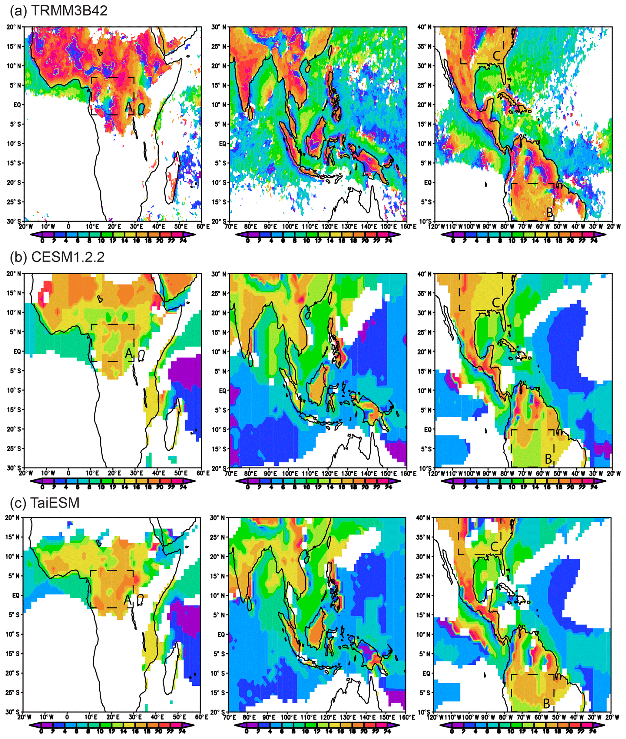
Figure 1Peak phase of diurnal rainfall cycle over three major tropical regions: central Africa, southeast Asia, and Amazonia in (a) TRMM3B42 (2001–2011), (b) CESM1.2.2 (1979–2005), and (c) TaiESM (1979–2005). Areas with an amplitude of diurnal precipitation smaller than 0.5 mm d−1 are masked out.
Similar to that in E3SM, improvement in the diurnal rainfall cycle is found in TaiESM. Figure 1 displays local times (LTs) of the diurnal rainfall peak occurrence, referred to as the peak phase from the 11-year (2001–2011) Tropical Rainfall Measuring Mission (TRMM) merged satellite data (Huffman et al., 2007) and the historical model runs during 1979–2005. Areas with an amplitude of diurnal rainfall cycle smaller than 0.5 mm d−1 are masked to emphasize the regions with strong diurnal rainfall signals. Two distinct changes in diurnal rainfall cycle are found in TaiESM compared with those in CESM1.2.2. First, the simulated diurnal rainfall peak over the tropical land areas is improved. For example, the observed peaks in the central Africa (Box A) and the Amazon Basin (Box B) occur around 20:00–22:00 and 18:00–20:00 LT, respectively. These peaks are delayed from 12:00–14:00 LT in CESM1.2.2 to 14:00–18:00 LT in TaiESM. A similar delay is also found in islands such as Borneo and Sumatra. As a result, nocturnal rainfall in TaiESM is increased compared with that in CESM1.2.2.
Second, the propagation of convective organizations is better simulated. Propagating convective systems originating from coastlines or topographical regions could be demonstrated by the gradual phase change in Fig. 1, such as the eastern slope of the Rocky Mountains (Box C) and northern South America (north of Box B). More specifically, Fig. 2 shows the Hovmöller diagram of longitude and local time for TaiESM, CESM1.2.2, and TRMM observations over SGP (35–40∘ N, 90–110∘ W) in Box C. Convection occurs at 104∘ W in the evening and propagates eastward in the observation (Carbone and Tuttle, 2008). In CESM1.2.2, convection occurs in the early afternoon and peaks before midnight, but it is stationary at the same location. TaiESM successfully captures the eastward propagation of the rainfall and a better occurrence time of convection in the late afternoon, as well as the more realistic rainfall intensity. This result is consistent with the single-column model tests of Y.-C. Wang et al. (2015), indicating that their proposed convective trigger may be the cause of these improvements. Furthermore, Wang and Hsu (2019) demonstrate that the improvement of nocturnal rainfall over SGP is mainly from the superior response of the ULL + CIN convective trigger to the low-level convergence between the branch of the mountain–plain solenoid and low-level jet from the Gulf of Mexico. With the horizontal resolution on the order of 100 km, this result suggests that the convective trigger of TaiESM captures the large-scale preconditioning related to the convective organization there (Dirmeyer et al., 2011) rather than only the convective systems itself.
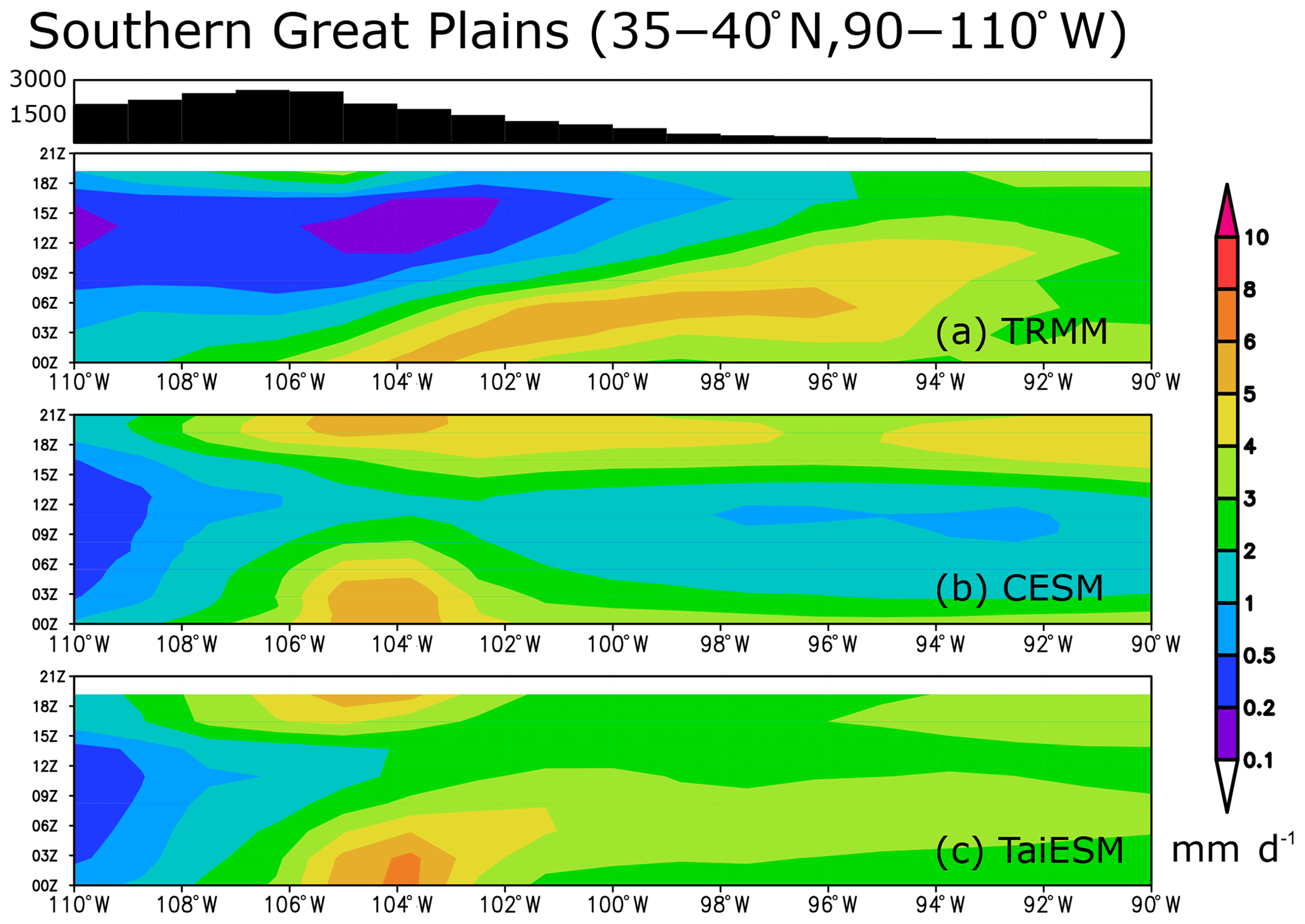
Figure 2Time–longitude Hovmöller diagrams for diurnal rainfall cycle over the SGP observed by the TRMM3B42 dataset (2001–2011, a) and simulated by CESM1.2.2 (b) and TaiESM (c), with the elevation of topography on top.
2.1.2 Cloud fraction
The cloud macrophysics scheme used in TaiESM is the GFS–TaiESM–Sundqvist (GTS) scheme (Shiu et al., 2020). Its prototype was first developed for the NCEP GFS model and has been further modified for the TaiESM. Similar to that in many numerical weather prediction and global climate models, the GTS scheme is based on the Sundqvist scheme (Sundqvist et al., 1989), which calculates changes in cloud condensates in a grid box on the basis of the budget equation for relative humidity (RH) with large-scale advection. The CAM5 macrophysics (Park et al., 2014) follows this approach and assumes empirical values of critical RH (RHc) as the threshold of condensation. The key difference of the GTS scheme from the CAM5 macrophysics is the re-derivation of the equation relating the change in the subgrid-scale cloud condensate using the distribution width of the mixing ratio of total water (qt) to replace RHc, as indicated in Tompkins (2005). The unnecessary use of RHc is consequently removed to allow an improved correlation among cloud fraction, RH, and condensates.
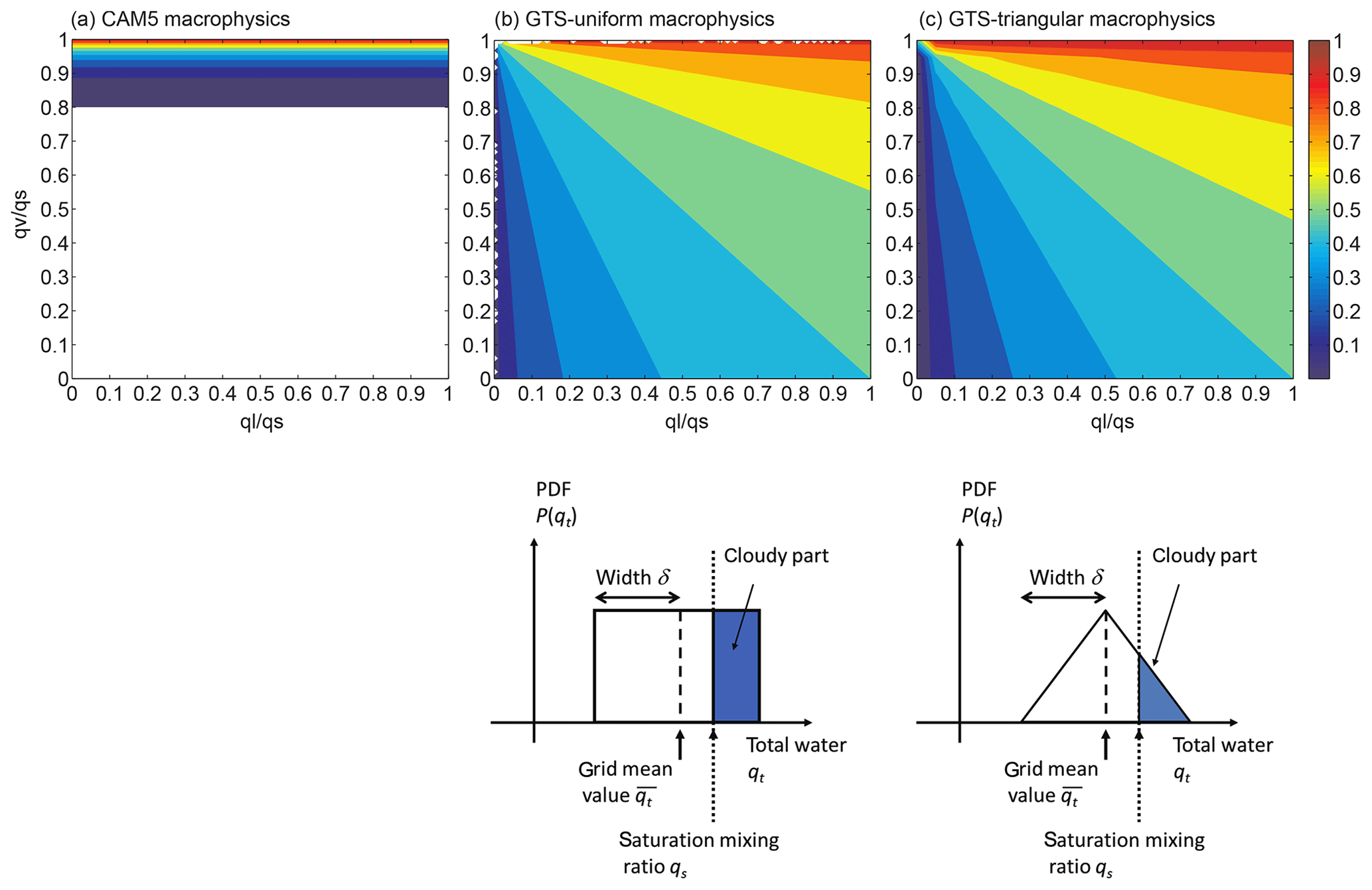
Figure 3Theoretical calculations of cloud fraction as a function of RH for water vapor and condensates: (a) CAM5 macrophysics scheme, (b) GTS macrophysics with uniform PDF, and (c) GTS macrophysics with triangular PDF.
Figure 3 illustrates cloud fraction as a function of RH of water vapor (qv∕qs) and RH of condensates (ql∕qs) for the CAM5 macrophysics and the GTS schemes with uniform and triangular probability density functions (PDFs) of qt in a grid box. Given the same RH of water vapor, the PDF-based calculation allows larger cloud fraction if more cloud condensates exist in the grid box than the CAM5 macrophysics. The difference in cloud fraction produced by the two PDFs is small, implying that this scheme might not be very sensitive to the shape of the distribution. The triangular PDF additionally provides rapid changes in cloud fraction when the RH of condensates and water vapor changes, and it is used as the default PDF of the GTS scheme.
2.1.3 Aerosol
The aerosol parameterization used in TaiESM is the Statistical-Numerical Aerosol Parameterization (SNAP; Chen et al., 2013). SNAP is a bulk parameterization, and the modal approach (Seigneur et al., 1986; Whitby and McMurry, 1997) is adopted to describe the particle size distribution. In contrast to conventional aerosol parameterizations in most ESMs, changes in the zeroth moment (number), second moment (surface area), and third moment (mass) due to physical processes are tracked in SNAP. The physical processes included in SNAP are emission, nucleation, coagulation, condensation, mixing, and dry and wet deposition. SNAP has been applied to the US EPA Models-3/Community Multi-scale Air Quality (CMAQ; Byun and Schere, 2006) modeling system and been verified by observations (Chen et al., 2013; Tsai et al., 2015) with the Weather Research and Forecasting Model (WRF; Skamarock et al., 2005).
2.2 Land
The land model in TaiESM is CLM4 (Oleson et al., 2010; Lawrence et al., 2011). The surface albedo is primarily a function of vegetation, soil moisture, solar zenith angle, and snow reflectivity calculated by the Snow, Ice, and Aerosol Radiative Model (SNICAR; Flanner and Zender, 2006), which considers the aerosol deposition of black carbon and dust, effective size of snow grains, and vertical profile of heating. As the albedo of a grid box is determined, it is then adjusted to include the topographic effect on surface solar radiation.
The parameterization for 3D radiation–topography interactions is to evaluate the impact of topography on surface solar radiation, including insolation on various slopes and aspects, shadow cast by nearby mountains, and reflections between surfaces (Lee et al., 2013). It is developed on the basis of numerous “exact” Monte Carlo calculations that simulate the scattering, reflection, and absorption of photons within the 3D atmosphere and surface (Chen et al., 2006; Liou et al., 2007; Lee et al., 2011). The parameterization adjusts surface albedo so that the solar radiation absorbed by the surface in the land model corresponds to the results of the Monte Carlo calculation. Several geographic parameters are used for input, including the slope, aspect, sky view factor, terrain configuration factor, standard deviation of elevation within a grid box, and solar zenith and azimuth angles. Gu et al. (2012) and Liou et al. (2013) demonstrate that this topographic effect can increase the amount of snowpack in the valley and enhance the snowmelt in mountains in the WRF simulations over the western United States. Lee et al. (2015, 2019) also demonstrate that incorporating this parameterization into the Community Climate System Model version 4 (CCSM4) can significantly improve the surface energy budget over the Rocky Mountains and the Tibetan Plateau and thus reduce the systematic cold bias in the CMIP5 models.
2.3 Ocean, sea ice, and river
The sea ice and dynamic ocean components of TaiESM are from the CICE4 (Hunke and Lipscomb, 2008) and POP2 (Smith et al., 2010) of Los Alamos National Laboratory, respectively. The River Transport Model (RTM; Oleson et al., 2010) is designed to route liquid and ice runoff to the ocean as one of the freshwater input to POP2. The configurations of CICE4, POP2, and RTM in the fully coupled TaiESM simulations are identical to those in CESM1.2.2. Note that there is no land ice model in TaiESM. Therefore, the formation of sea ice from the discharge of the ice sheet to the ocean is not simulated.
To save computational resources, a zero-dimensional slab ocean model without dynamical process is commonly used to simulate the thermodynamic interaction between the atmosphere and ocean. In TaiESM, an efficient 1D mixed-layer model is coupled with the atmosphere component to reveal the impact of the fast evolution in upper-ocean layers. The one-column ocean model Snow–Ice–Thermocline (SIT; Tu and Tsuang, 2005; Tsuang et al. 2009) is designed to simulate the sea surface temperature (SST) and upper-ocean temperature variations with a high vertical resolution, including cool skin, diurnal warm layer, and mixed layer of the upper ocean. SIT calculates changes in temperature, momentum, salinity, and turbulent kinetic energy driven by vertical fluxes parameterized using the classical K approach. Cool skin is derived by considering merely molecular transport for vertical diffusion of heat in the skin layer, where the skin layer thickness is calculated as described by Artale et al. (2002). Beneath the skin layer, eddy diffusivity is determined according to a second-order turbulence closure approach (Gaspar et al., 1990), and the 1 m vertical discretization is deployed down to a 10 m depth for resolving diurnal warm layer. Because of the lack of ocean circulation in the one-column ocean model, the calculated ocean temperatures are weakly nudged to climatology for ocean below 10 m depth to avoid climate drift. SIT and the atmospheric model exchange SST and fluxes at every time step in the tropics (30∘S–30∘ N), whereas climatological SST drives the atmospheric model elsewhere. Note that SIT is not integrated into the dynamic ocean model (POP2); therefore, fully coupled TaiESM simulations do not include SIT.
2.4 Model tuning
The preliminary version of TaiESM was very cold compared with CESM1.2.2 using the preindustrial greenhouse gas concentrations and aerosol emissions. The most apparent change was the significant increase in cloud cover, particularly low clouds, which was probably induced by GTS cloud macrophysics and SNAP aerosol schemes. Therefore, several parameters associated with cloud formation were adjusted to reduce shortwave cloud forcing. We first explored that aerosol–cloud interactions were very strong in TaiESM with the SNAP scheme. Therefore, the activation rate of aerosols to cloud condensation nuclei was reduced by 10 % in the microphysics scheme to weaken the aerosol indirect effect. The sizes of detrained liquid particles from shallow convection and solid particles from deep convection were increased from 10 µm in CESM1.2.2 to 14 µm and from 15 to 25 µm, respectively. Larger detrained particles have smaller cloud optical depth and shorter suspension time in the air when the detrained water content is the same. Both effects can reduce cloud albedo. Although RHc is removed from the GTS scheme for grid boxes with the presence of condensates, it is still required for the formation of clouds in a cloud-free grid box. The value of RHc was increased from 0.8 in the free atmosphere in CESM1.2.2 to 0.85 in TaiESM to make cloud formation less efficient. After these adjustments, the global mean surface temperature of TaiESM in the preindustrial simulation is comparable to that of CESM1.2.2 while the radiation imbalance at the top of the atmosphere (TOA) is minimized. Note that this model tuning is made only at the spatial resolution of about 1∘. Additional tuning would be required for stable simulations at higher or lower resolutions.
The horizontal resolution of the atmosphere and land in TaiESM is 0.9∘ latitude by 1.25∘ longitude, with 30 vertical layers and a model top at 2 hPa in the atmosphere. The ocean and sea ice components use the same horizontal resolution with 320×384 grid points (approximately 1∘) and 60 vertical layers in the ocean. TaiESM is spun-up using CMIP5 preindustrial conditions, such as greenhouse gas concentrations, surface aerosol emissions, solar constant, and land-use types. Because TaiESM is considerably similar to CESM1.2.2, we use the model restart files of CESM1.2.2 for the 1850 control run as the initial condition to reduce the computational effort, particularly for the ocean component that may need more than 1000 years to reach a steady state. The spin-up integration continues for 500 years, and the climate state at the end of year 500 is used as the initial condition for the 500-year preindustrial control (hereafter piControl) simulation. The historical simulation then starts at the end of piControl (i.e., year 1000) with observationally based forcing, including changes in the solar constant, greenhouse gas concentrations, surface aerosol emission, and volcanic eruptions, from 1850 to 2005.
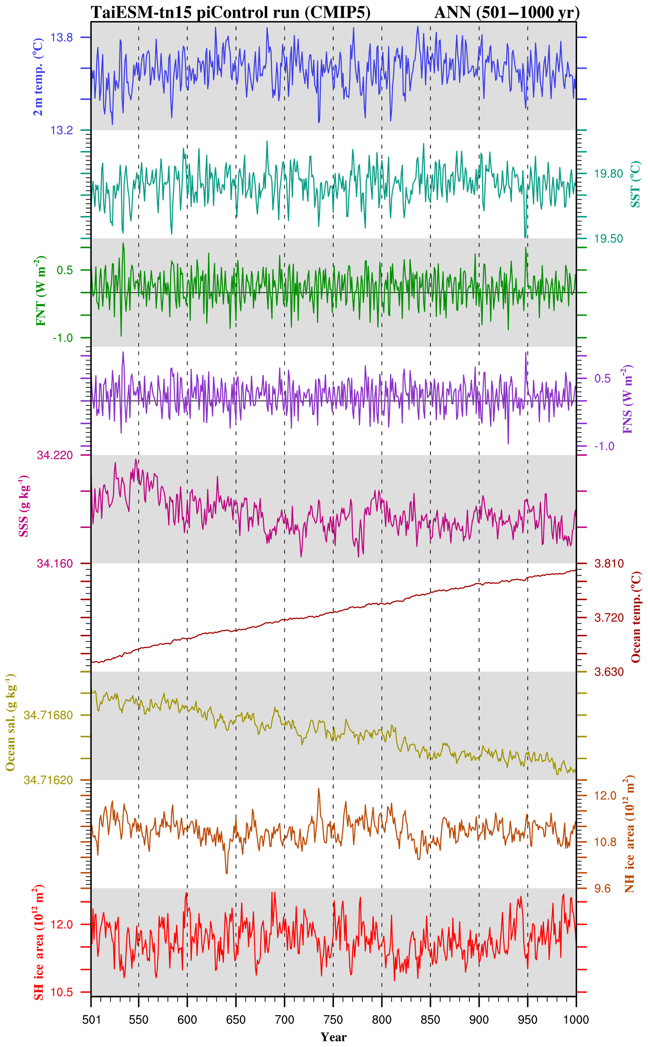
Figure 4A 500-year time series of annual mean climatological quantities in TaiESM piControl simulation (from top to bottom): SAT at 2 m height, SST, net flux at the TOA (FNT), net flux at the surface (FNS), SSS, volume-averaged ocean temperature, volume-averaged ocean salinity, and NH and SH sea ice areas. The horizontal lines in FNT and FNS indicate the zero value.
In this section, the global means of several climatological variables in the piControl run of TaiESM are evaluated. The climate drift from CESM1.2.2 initial conditions to TaiESM equilibrium during the spin-up is also assessed to represent differences between the two models caused by the new or modified physical processes in TaiESM.
4.1 Time series of climate states
Figure 4 illustrates the time series of several global mean variables in TaiESM piControl. The long-term global mean TOA net flux is 0.086 W m−2, and it decreases by 0.0054 W m−2 in 500 years, but insignificantly. Furthermore, the mean surface net flux is 0.081 W m−2 with an almost identical decreasing trend as TOA net flux. The imbalance at TOA causes heating of the whole model system, and the comparatively smaller imbalance at the surface indicates that a smaller part of excessive energy remains in the atmosphere in piControl. Consequently, the long-term trend of surface air temperature (SAT) is 0.0088 K century−1 in 500 years, which is statistically significant. By contrast, the trend of SST is 0.0047 K century−1, only about half of the SAT trend and insignificant. By breaking down the surface net flux, we found that the energy exchange between the atmosphere and land is less than 10−5 W m−2, whereas the net flux into the ocean is 0.114 W m−2 (figures not shown). The excessive energy enters the deep ocean and leads to a steady increase in global mean ocean temperature of 0.030 K century−1. Therefore, even after a 1000 years' simulation, the system does not reach the thermodynamic equilibrium. In addition, considering that the heat capacity of the entire ocean is approximately 1000 times larger than the atmosphere, the heating rates of the atmosphere caused by the residual net flux (0.005 W m−2) are too small compared with the heating rate of the ocean. It implies that an unknown energy leak may exist in the coupling between the atmosphere and ocean, which requires further investigation in programming to fix this problem.
The annual mean time series of sea ice area in the Northern Hemisphere (NH) and Southern Hemisphere (SH) are exhibited in the bottom panels of Fig. 4. The Arctic sea ice has a small but significant trend of km2 century−1, corresponding fairly well to the slight warming of the entire model. By contrast, the linear trend of the sea ice area in the Southern Ocean over the 500-year span is almost 0, even though the variation is much larger. The minimal change in the sea ice area indicates that the energy gain of the cryosphere could be negligible compared with other model components. The global mean sea surface salinity (SSS) reduces significantly by −0.0036 g kg−1 century−1. However, it can be found that SSS is almost constant with a slope of about 10−4 g kg−1 century−1 after year 700. On the other hand, there is a small but significant decreasing trend of the global mean ocean salinity of g kg−1 century−1, which is very close to the trend of SSS in the last 300 years.
Table 1Long-term global means of selected climatological variables from CESM1.2.2 and TaiESM
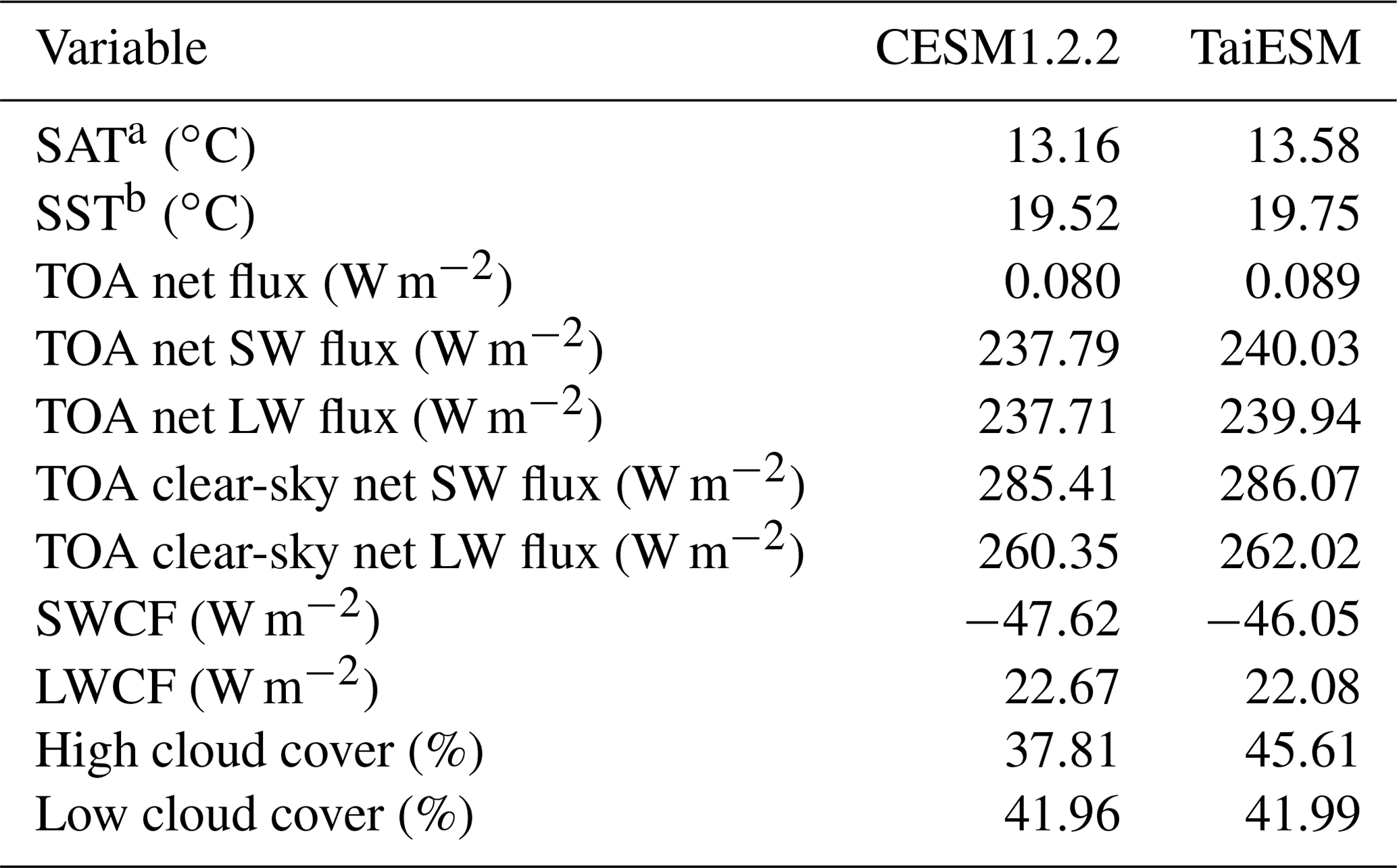
a Estimated observation value of SAT is 13.63 ∘C from BEST (Rohde et al., 2013). b Estimated observation value of SST is 19.27 ∘C in 1854 from Extended Reconstructed Sea Surface Temperature (ERSST; Huang et al., 2017)
4.2 Comparison with CESM
The long-term means of several variables in piControl runs performed by CESM1.2.2 and TaiESM are listed in Table 1. The TOA net flux in TaiESM and CESM1.2.2 are both within 0.09 W m−2. The magnitude of imbalance is acceptable, but it could lead to warming of the entire Earth system. The SAT and SST in TaiESM are higher than those in CESM1.2.2 by 0.42 and 0.23 K, respectively. Shortwave (SW) net flux at TOA in TaiESM is larger than CESM1.2.2 by 2.24 W m−2, which might be the primary cause of higher surface temperatures and consequently result in larger longwave (LW) net flux at TOA of 2.23 W m−2. The difference in the clear-sky net SW flux at TOA is only 0.66 W m−2, suggesting that the surface albedo difference is small, whereas the contribution from the difference in cloud reflection is larger. Although the high and low cloud covers in TaiESM are larger than those in CESM1.2.2, the magnitude of SW cloud forcing (SWCF) is smaller in TaiESM. It indicates that clouds in TaiESM are less reflective than that those in CESM1.2.2. By contrast, the differences in clear-sky net LW flux at TOA and LW cloud forcing (LWCF) are 1.67 and 0.59 W m−2, respectively; therefore, the warmer surface and atmosphere have greater contribution to additional outgoing longwave radiation (OLR) in TaiESM. However, the amount of high cloud in TaiESM is substantially larger than that in CESM1.2.2. This implies that the high clouds in TaiESM could be optically thinner. The different relation between cloud forcing and cloud cover in SW and LW in TaiESM is probably due to the GTS scheme, which can produce a larger fraction but less dense clouds compared with the cloud macrophysics scheme in CAM5.
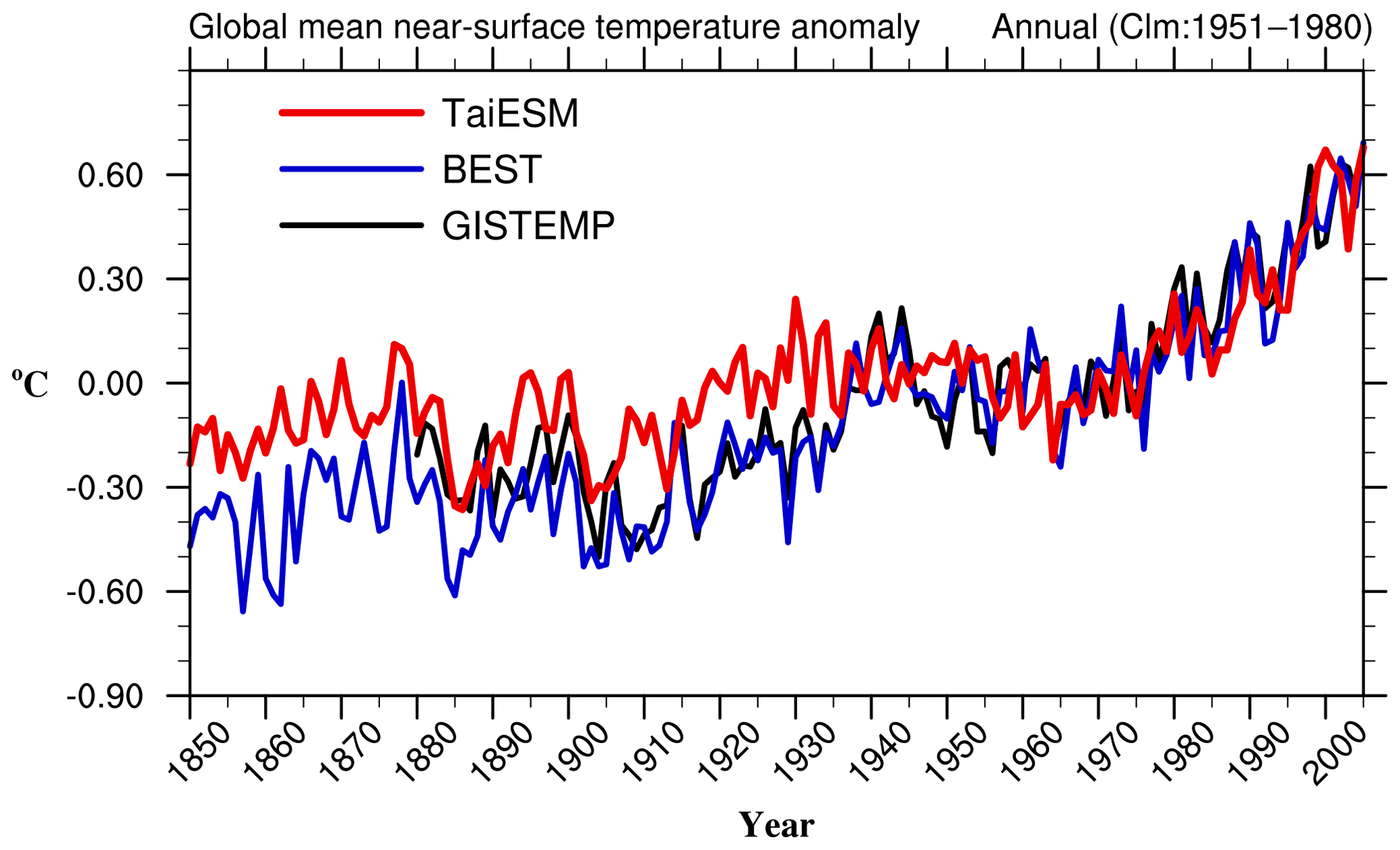
Figure 5Historical global mean SAT anomalies relative to the period of 1951–1980 from TaiESM historical simulation (red) and observational datasets of BEST (blue) and GISTEMP (black).
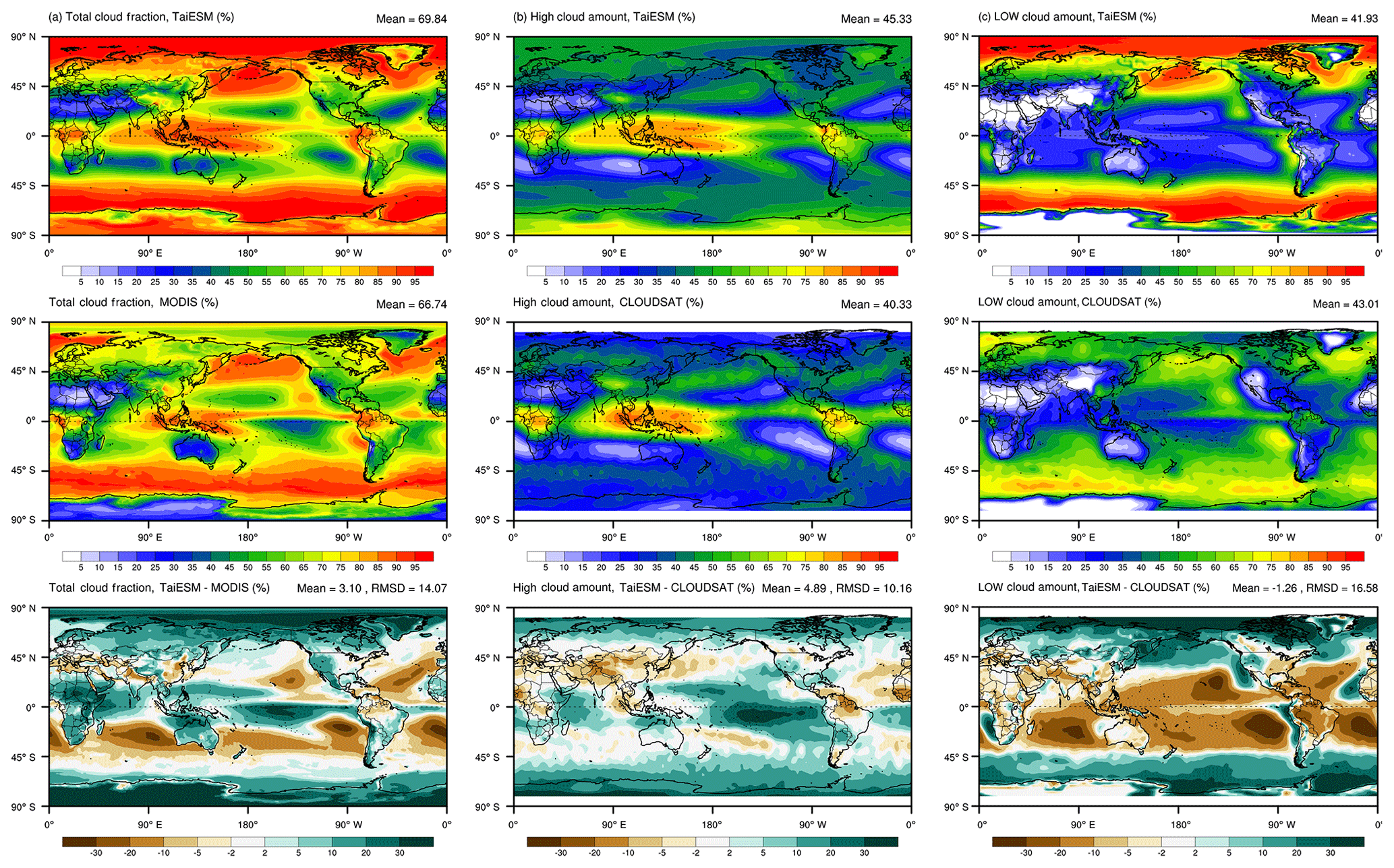
Figure 6Vertically integrated cloud fractions for (a) total cloud, (b) high cloud, and (c) low cloud in the 1979–2005 TaiESM historical run (top row), observations (MODIS for total cloud and CloudSat–CALIOP for high and low cloud, central row) and biases (bottom row).
In this section, we evaluate the performance of the TaiESM historical simulation against the observation or reanalysis data. The temporal evolution of global mean temperature from the preindustrial period to the present day is assessed. In the historical simulation, the mean states of the current climate, defined as the period of 1979–2005, are used for comparison. The behavior of the El Niño–Southern Oscillation (ENSO) in TaiESM is also evaluated.
5.1 Global mean temperature evolution
Figure 5 illustrates changes in the global mean near-surface temperature anomaly of TaiESM and two observations – Berkeley Earth Surface Temperature (BEST; Rohde et al., 2013) and Goddard Institute for Space Studies Surface Temperature (GISTEMP; Lenssen et al., 2019) – by using the mean temperature of 1951–1980 as the benchmark. The warming trend of TaiESM is weaker than the observation data during 1850–1935. The evolution of SAT in TaiESM exhibits fluctuation similar to observations, particularly before 1900, but with smaller amplitudes. The magnitudes of cooling induced by major volcanic eruptions, such as Krakatoa (1883), Santa Maria (1902), Agung (1963), and Pinatubo (1991), in TaiESM is close to those in the observational data, implying that the radiative forcing due to stratospheric aerosols is in good agreement with the observations. After 1950, the change in SAT of TaiESM follows the observations and captures the trend of global warming very well. The warming rate of TaiESM during 1950–2005 is 1.12 K century−1, comparable with 1.16 and 1.27 K century−1 of BEST and GISTEMP, respectively.
5.2 Cloud and radiation
Figure 6a demonstrates the comparison in the total cloud fraction between TaiESM and the Moderate Resolution Imaging Spectroradiometer (MODIS) Level 3 product during 2001–2012. TaiESM overestimates the total cloud fraction by approximately 3 % globally with a root-mean-square difference (RMSD) of 14.07. Almost all of the Arctic Ocean is overcast in TaiESM, which is approximately 30 % higher than observational data. Cloud fraction is also severely overestimated over the Antarctic continent and the Southern Ocean. TaiESM produces too much cloud over the southern branch of the Intertropical Convergence Zone (ITCZ) in the central and eastern Pacific, implying the prevalence of double ITCZ, which will be discussed in a subsequent section. An excessive amount of clouds is also noted in the Maritime Continent, western equatorial Indian Ocean, and most of the land areas. By contrast, cloud fraction is remarkably underestimated in the Amazon Basin and the subtropical ocean, particularly the stratocumulus near the western coasts of continents. Compared with the synergic CloudSat and Cloud-Aerosol Lidar with Orthogonal Polarization (CALIOP) data during 2006–2010 (Kay and Gettelman, 2009), low clouds in TaiESM are systematically underestimated over the entire tropical and subtropical regions, as shown in Fig. 6c, whereas they are overestimated in high-latitude areas. The total cloud fraction in the tropics is high because of excessive high cloud in the model (Fig. 6b).
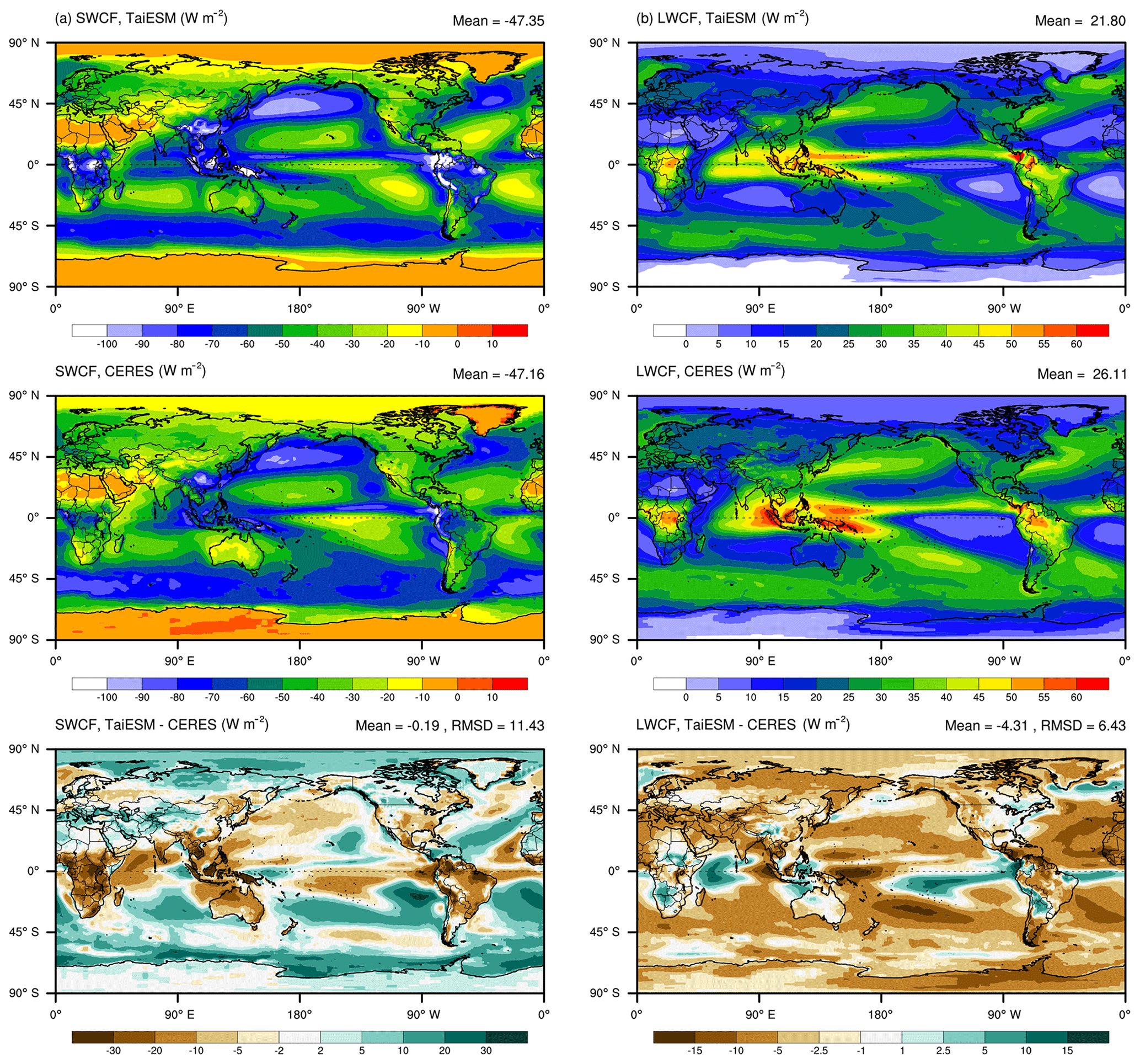
Figure 7Cloud forcing for (a) shortwave and (b) longwave in the 1979–2005 TaiESM historical run (top panels), observations (central panels, CERES–EBAF), and biases (bottom panels).
Clouds can substantially modulate the radiation field because of its high reflectivity in SW and high absorptivity in LW. Figure 7a illustrates the comparison of SWCF in TaiESM with that in Clouds and the Earth's Radiant Energy System–Energy Balanced and Filled data (CERES–EBAF; Kato et al., 2018) over 2000–2015. In terms of the global mean, SWCF in TaiESM is very close to that of the observational data with a difference of only 0.19 W m−2. Although there is excessive cloud over the polar regions in TaiESM, such as the Southern Ocean near the Antarctic continent and almost all of the Arctic Ocean, SWCF is not as strong as that in the observational data. It could be contributed from the optically thin polar clouds due to the GTS cloud macrophysics scheme and from the positive bias of sea ice albedo in the Arctic Ocean in TaiESM (not shown). In the subtropical and tropical regions, SWCF generally follows the spatial pattern of total cloud fraction – i.e., a larger cloud fraction produces stronger SWCF, such as the storm track in the North Pacific, southern branch of ITCZ, Maritime Continent, western tropical Indian Ocean, and south of the Sahara Desert. However, SWCF is too strong over the Amazon Basin in TaiESM, even though there is an underestimated amount of clouds. By contrast, because of the underestimated total cloud fraction, SWCF in TaiESM is too weak over the stratocumulus areas off the California and Peru coasts as well as over the subtropical Pacific, Atlantic, and Indian oceans in the SH.
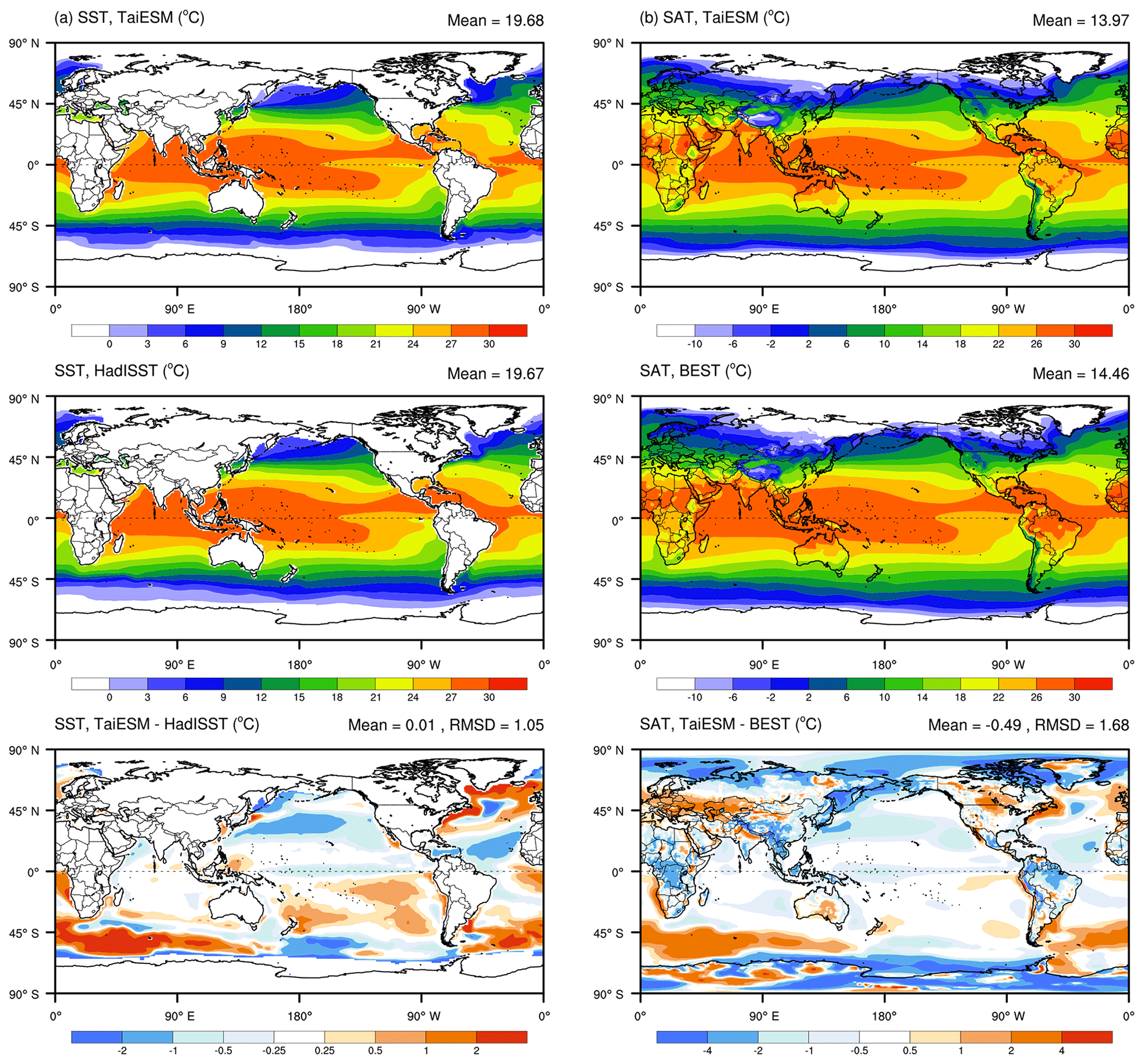
Figure 8(a) SST and (b) SAT in the 1979–2005 TaiESM historical run (top panels), observations (HadISST for SST and BEST for SAT, central panels), and biases (bottom panels).
The global mean of LWCF in TaiESM is significantly weaker (by 4.31 W m−2) than that in CERES–EBAF. As illustrated in Fig. 7b, TaiESM underestimates LWCF worldwide, and the magnitude of the LWCF bias generally follows the bias of high cloud. Positive LWCF bias only exists in some regions over the tropical ocean with too many high clouds in TaiESM. However, although more high clouds exist along the northern branch of the ITCZ, LWCF is weaker in the model. The remarkable negative LWCF bias seems incompatible with the overestimated high clouds because more high clouds should be able to intercept more LW radiation from the surface. This inconsistency is probably due to the lower altitude of the high clouds or the less dense clouds in TaiESM.
5.3 Surface temperature
Figure 8a illustrates the comparison of SST between TaiESM and the Hadley Centre Sea Ice and Sea Surface Temperature dataset (HadISST; Rayner et al., 2003). The regions with a long-term mean sea ice concentration larger than 15 % are not used for calculations of the mean and RMSD. The global mean bias of SST in TaiESM is 0.01 K with an RMSD of 1.05 K. The overestimated SST over the Southern Ocean and subtropical South Pacific is probably induced by additional downward SW radiation because of the inaccurate microphysical properties of polar clouds (Kay et al., 2016) and the negative bias of cloud fraction as shown in Fig. 6a. The warm bias in the major upwelling regions off the western coasts of the Americas and Africa is a common deficiency in many climate models (Griffies et al., 2009), caused by insufficient spatial resolution of the atmosphere and ocean. Warm bias can also be found in the North Atlantic including the coast of North America, the Labrador Sea, and south of Greenland. Negative biases exist in most of the North Pacific and subtropical North Atlantic, probably because of overestimated wind stress in these regions.
Although the SST bias in TaiESM is very small, the global mean SAT in TaiESM is substantially colder than the observational data (by 0.49 K with an RMSD of 1.68 K). This result indicates that the temperature over land and sea ice in TaiESM is severely underestimated (Fig. 8b). Cold bias exists over most of the polar regions, the Tibetan Plateau, and tropical land areas (e.g., Amazonia, central Africa, and southeast Asia). It must be due to the excessive cloud that reflects excessive sunlight. SAT bias over the ocean generally follows SST bias, except that the SAT bias in the subtropical South Pacific is very small despite the warm SST bias.
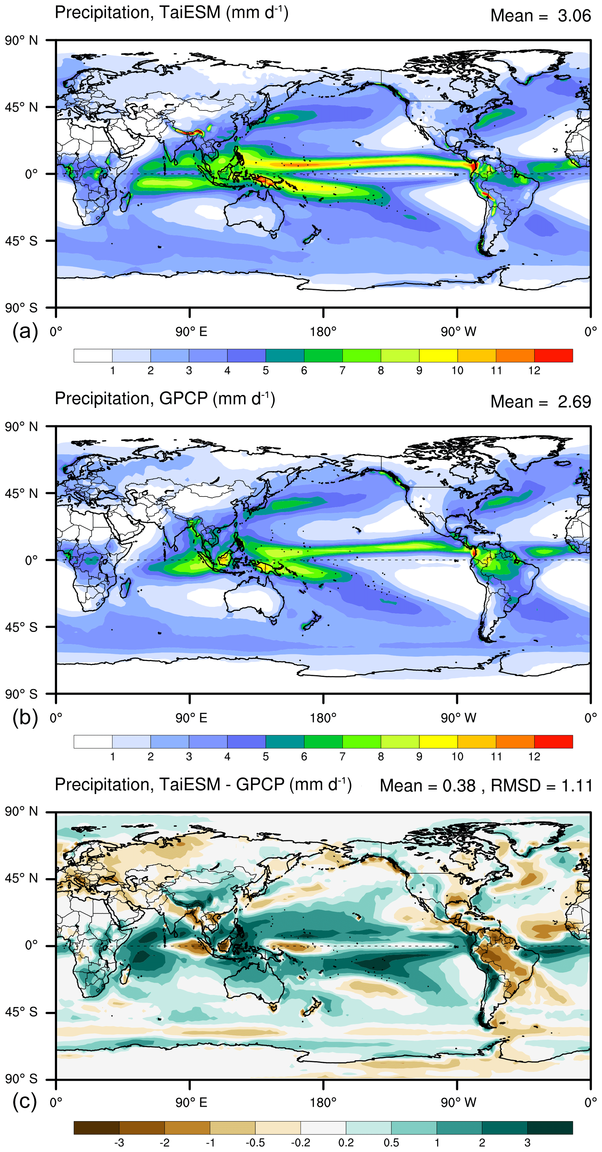
Figure 9Precipitation in the 1979–2005 TaiESM historical run (a), observations (GPCP, b), and biases (c).
5.4 Precipitation
Figure 9 illustrates the mean precipitation over 1979–2005 in TaiESM and Global Precipitation Climatology Project (GPCP; Huffman et al., 2009) 1-Degree Daily (1-DD) data. TaiESM overestimates the global precipitation by 0.38 mm d−1 with an RMSD of 1.11 mm d−1. The most pronounced bias in TaiESM is the double ITCZ – a common issue in most contemporary GCMs (Lin, 2007; Hirota and Takayabu, 2013) and in CESM1 (C.-c. Wang et al., 2015). The precipitation rates of both the northern and southern ITCZ branches are extremely strong. The overly intense convection strengthens the subsidence and consequently produces too little rainfall along the Equator. Precipitation is also overestimated in the Maritime Continent, while it is severely underestimated in Borneo. In TaiESM, the land–sea contrast in precipitation is not as apparent as in the observation over the warm pool region. The South Pacific convergence zone (SPCZ) is also too strong and too parallel to the ITCZ. The dipole bias in the tropical Indian Ocean, excessive rainfall in the western part and scant rainfall in the eastern part, still exists as in NCAR models (Gent et al., 2011). There is also a double ITCZ bias in the Atlantic Ocean in that the southern branch is too strong and the northern branch is too weak. In South America, precipitation over the Amazon Basin is considerably underestimated, whereas excessive orographic precipitation can be found along the Andes (Cook et al., 2012).
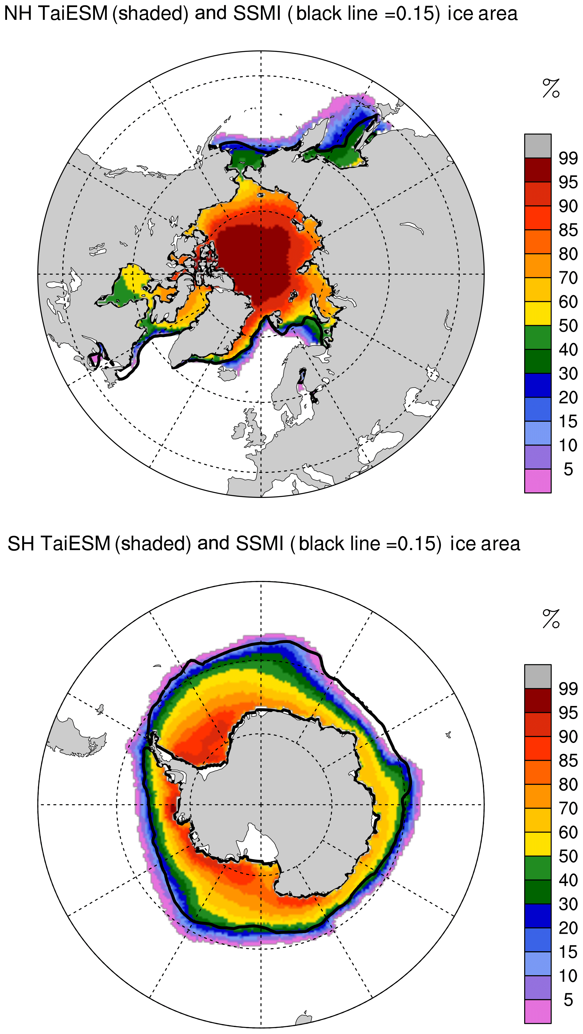
Figure 10Annual mean sea ice concentration in the 1979–2005 TaiESM historical run for both NH and SH. The solid black lines indicate the 15 % sea ice concentration from the observation (NSIDC–CDR, 1979–2005).
5.5 Sea ice
Figure 10 presents the annual mean of sea ice concentration in the Arctic Ocean and Southern Ocean in TaiESM, and the black lines indicate the 15 % mean concentration from the National Snow and Ice Data Center (NSIDC) Climate Data Record (CDR) of passive microwave sea ice concentration version 3 (Peng et al., 2013), during 1979–2005. In the NH, TaiESM severely overestimates sea ice concentration over the North Pacific, particularly in the Sea of Okhotsk. TaiESM also overestimates sea ice in the Barents Sea and near the east coast of Greenland but slightly underestimates sea ice in the Labrador Sea. In the SH, sea ice in TaiESM is generally in agreement with the observation. Excessive sea ice is noted in the area south of New Zealand, but in the Indian Ocean region, sea ice is scant. This deviation follows the SST bias presented previously.
Figure 11 illustrates the temporal evolution of the annual sea ice concentration in TaiESM compared with that in the CDR. The change in NH sea ice in TaiESM generally captures the trend in the observation before 2002. However, there is an increase in TaiESM in the last 4 years, in contrast to an accelerated reduction in observational data. This sea ice increase could be a fluctuation in a climate simulation, and it requires longer integration for additional investigation. In the SH, a decreasing trend of the sea ice concentration can be found in TaiESM, whereas it remains almost unchanged in observational data. Because there is no land ice model in TaiESM, the discharge of the ice sheet from the Antarctic continent to the Southern Ocean, the major source of SH sea ice, cannot be simulated accurately. Consequently, the sea ice concentration in the SH could be controlled primarily by temperature in TaiESM, leading to an unrealistic temporal evolution.

Figure 11Time series of annual mean total sea ice area for both NH and SH from TaiESM historical run and observation.
5.6 ENSO
To evaluate the ENSO behavior during 1976–2005 in TaiESM, the HadISST sea surface temperature and MRE2 reanalysis data in the same period are used. The observed and simulated spectra of the Nino 3.4 index presented in Fig. 12 reveal the adequate ability of TaiESM in reproducing the periodicity of El Niño. The observed Nino 3.4 index exhibits three statistically significant peaks between 2 and 6 years. TaiESM is able to simulate three spectral peaks with slightly shorter periods, while the amplitudes of all three peaks are larger than observations.
The anomalies of surface temperature, sea level pressure, and near-surface wind in December–February when the ENSO is at the mature stage are shown in Fig. 13, which is the composite of five and six El Niño events in observation and TaiESM simulation, respectively. The simulated SST anomaly (SSTA) is evidently larger in both amplitude and spatial coverage than the observed one and with the maximum shifted westward to the central equatorial Pacific compared with the observation, which is the common bias in many climate models. The horseshoe-like negative SSTA in the northwest, southwest, and west of the positive SSTA is stronger and covers much larger areas than the observed one. This over-simulated SSTA structure leads to some marked biases in the simulated atmospheric circulation and temperature, such as the cold bias in the western North Pacific and Maritime Continent, warm bias in the western Indian Ocean and Bering Sea, and too strong a convergence in the eastern equatorial Pacific.
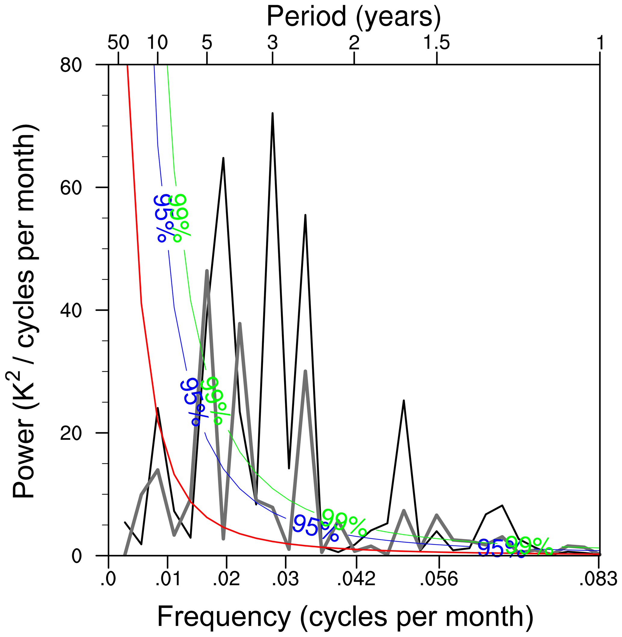
Figure 12Power spectra of Nino 3.4 index from TaiESM (thin black line) and HadISST (thick gray line) during 1976–2005. Color curves indicate the levels of significance at 99 % (green), 95 % (blue), and 90 % (red).
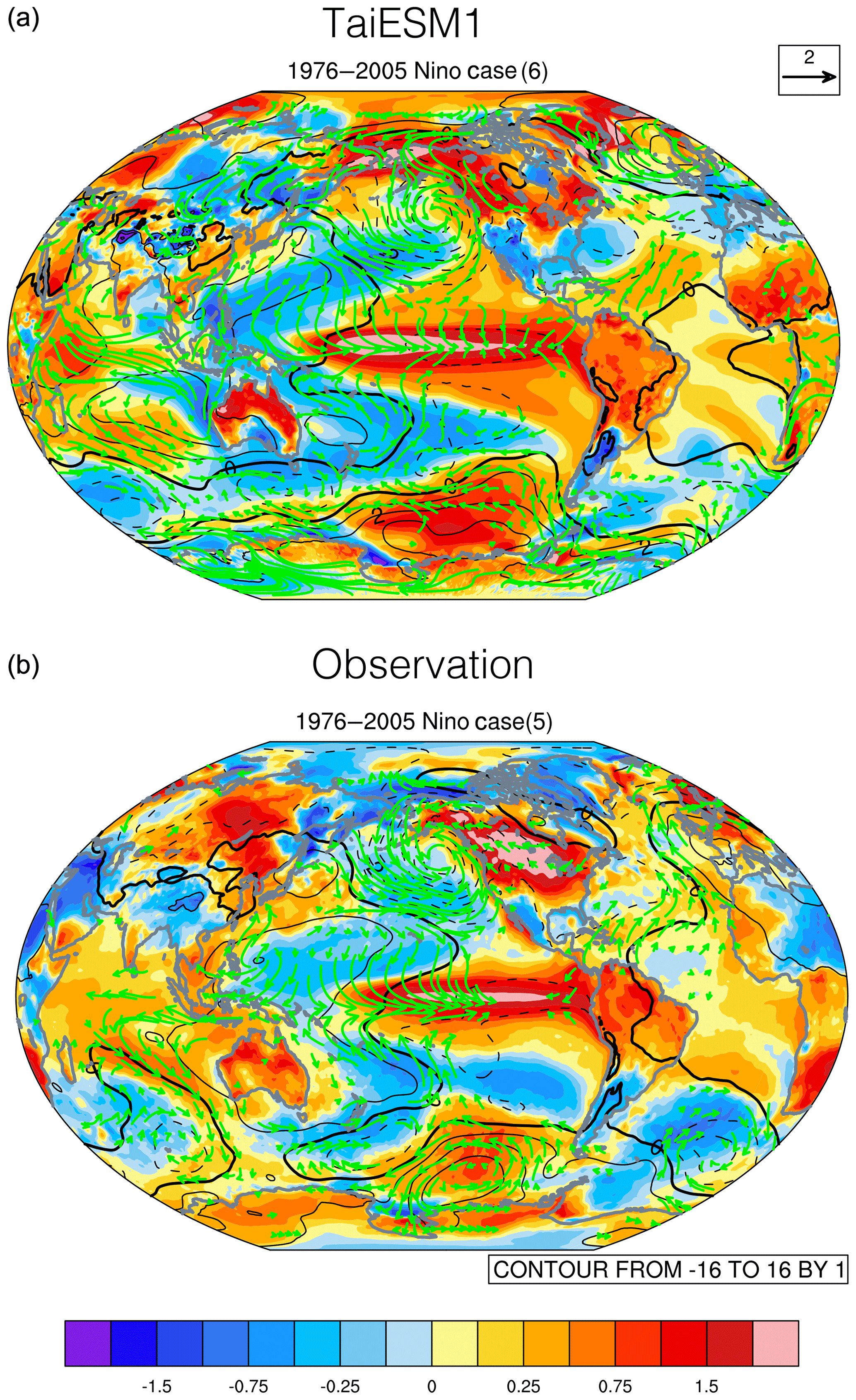
Figure 13Composite anomalies of surface temperature (shading), sea level pressure (contour), and near-surface wind (arrow) in December–February during El Niño years. There are six and five El Niño events during 1976–2005 in the TaiESM simulation (a) and observation (b), respectively.
5.7 Comparison with CMIP5 models
The overall performance of the TaiESM historical simulation during 1979–2005 is evaluated by comparing it with other CMIP5 models following the metrics introduced by Gleckler et al. (2008). Figure 14 shows the normalized space–time root-mean-square error (RMSE) of selected variables from TaiESM, several CMIP5 models, and a multi-model ensemble (MME) against reanalysis and observation datasets. The reference data of air temperatures (TA), zonal and meridional wind velocities (UA and VA), and geopotential height (ZG) at various pressure levels, as well as the surface air temperature (TAS), are from the Collaborative Reanalysis Technical Environment (CREATE) Multi-Reanalysis Ensemble version 2 (MRE2; Potter et al., 2018). The observational precipitation (PR) data are from GPCP. Upward longwave radiation in the total sky (RLUT) and clear sky (RLUTCS) and upward shortwave radiation in the total sky (RSUT) and clear sky (RSUTCS) are from CERES-EBAF. It is expected that the errors of CMIP5 MME are generally the smallest. TaiESM has the smallest bias in PR among all CMIP5 models, and its performance in RSUT and RLUT is also very good. The relatively poor performance in TAS is primarily due to the cold bias over land and sea ice areas. The RMSEs of all variables in TaiESM are smaller than the median CMIP5 error, indicating that the performance of TaiESM is above average among all CMIP5 models. The performance of TaiESM is comparable to that of CESM1-CAM5, and they have similar strengths and weaknesses. Note that three variables with an RMSE larger than the median in CESM1-CAM5 are all improved in TaiESM.
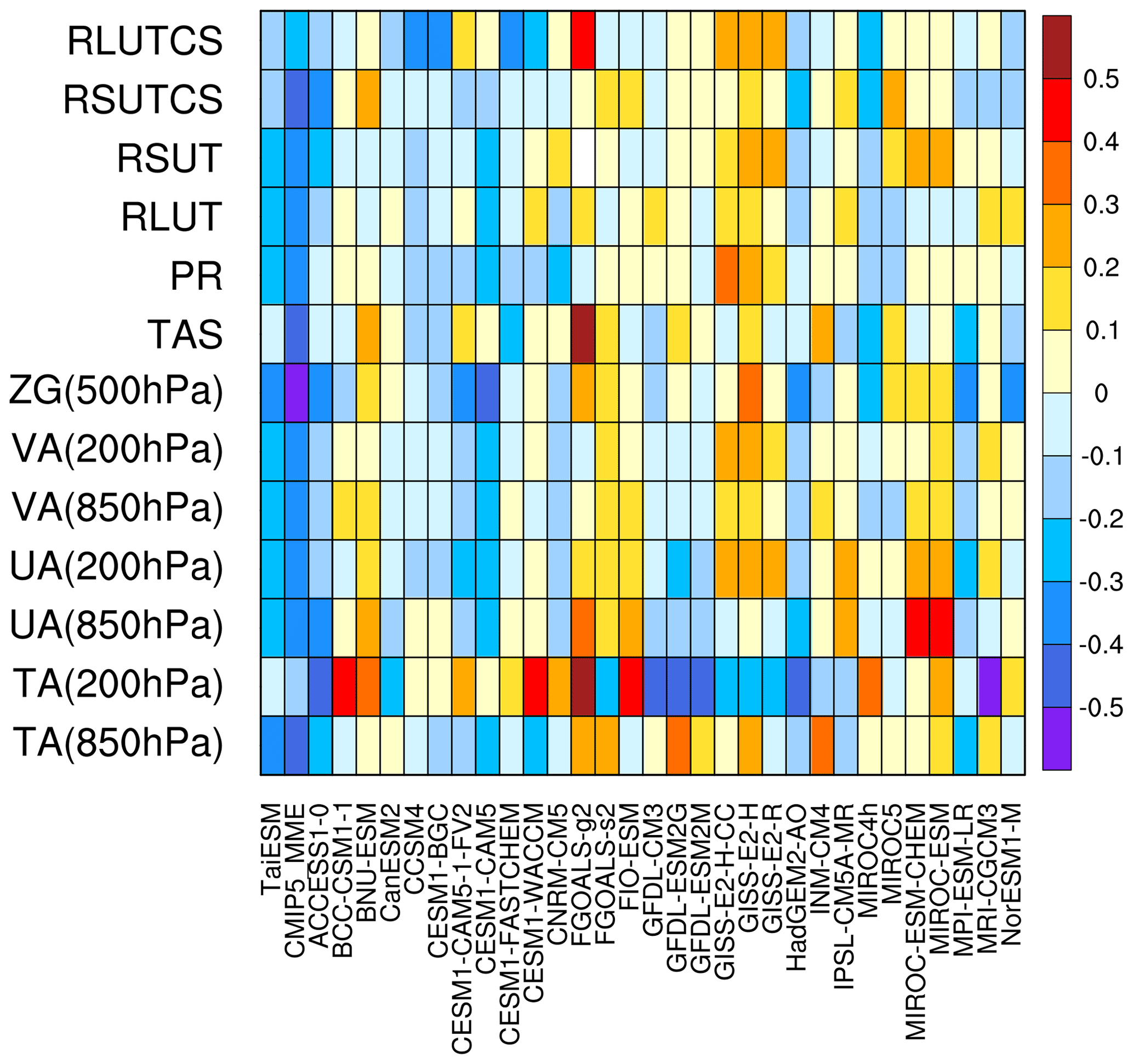
Figure 14The space–time RMSEs of upward longwave radiation at TOA in total sky and clear sky (RLUT and RLUTCS), upward shortwave radiation at TOA in total sky and clear sky (RSUT and RSUTCS), precipitation (PR), surface air temperature (TAS), geopotential height (ZG), meridional wind (VA), zonal wind (UA), and air temperature (TA) from TaiESM, CMIP5 models, and CMIP5 MME. The values of shading represent the magnitude of the normalized error with respect to the median CMIP5 error. For example, a value of −0.2 indicates that the RMSE of a model is 20 % smaller than the median error.
This paper documents the TaiESM version 1, developed on the basis of CESM1.2.2, with revised physical and chemical parameterizations, including (1) trigger functions for deep convection, which can improve the variability simulation in convective rainfall; (2) the GTS cloud macrophysics scheme to avoid an artificial RH threshold for cloud formation; (3) the three-moment SNAP aerosol scheme; (4) 3D radiation–topography interactions to account for the impact of shading and reflection on shortwave radiation in mountains. A 1D mixed-layer ocean model is incorporated into the atmosphere component to simulate the thermodynamic air–sea interaction, but it is not used for fully coupled simulations.
TaiESM stability is assessed using the 500-year piControl. Although constant imbalance in the net flux at the TOA exists, the drifts of global mean SAT and SST are very small, with long-term trends of 0.0088 and 0.0047 K century−1, respectively. The excessive energy enters the deep ocean and leads to continuous warming by 0.030 K century−1. The drifts in the sea ice concentration in both NH and SH are both small because of the nearly zero net energy flux from the atmosphere to sea ice. However, the global mean SSS and total ocean salinity both demonstrate significantly decreasing trends.
For the historical evolution of SAT, the warming of TaiESM from 1850 to 1935 is too weak compared with the observation. After 1950, TaiESM satisfactorily captures the trend of global warming with a heating rate of 1.12 K century−1 comparable to the observation of 1.16 K century−1.
The current climatology of TaiESM during 1979–2005 is generally in agreement with the observations. The overall performance of TaiESM is better than the median of CMIP5 models, particularly in that the RMSE of precipitation is smallest. There are too many clouds in TaiESM, whereas the SWCF and LWCF are mostly similar to and weaker than the observation, respectively. This result implies that the new cloud macrophysics scheme produces a larger amount of but optically thinner clouds. SST in TaiESM is very close to the observation, whereas SAT is significantly colder, implying remarkably underestimated SAT over land and sea ice surfaces. TaiESM produces excessive precipitation, and the biases of the double ITCZ and dipole in the tropical Indian Ocean exist, whereas there is a severe dry bias in the Amazon Basin. The trend of the NH sea ice concentration in TaiESM follows the observation well, whereas it might not capture the accelerating reduction in the 21st century. For the ENSO simulation, TaiESM is able to reproduce three spectral peaks similar to observation with periods between 2 and 6 years, while the variability of SST, including the magnitude of the anomaly and spatial coverage, is too strong.
This paper focuses on the evaluation of the long-term climatological state and evolution of global mean quantities in TaiESM in preindustrial and historical simulations. The other part of the characteristics of an ESM, climate variability, is also very critical to the performance of a model, and it requires additional in-depth research. Further investigation of climate variability in TaiESM, including the intraseasonal oscillation, monsoon, and extreme precipitation, will be documented in follow-up papers.
The model code of TaiESM version 1 is available at https://doi.org/10.5281/zenodo.3626654 (Lee et al., 2020). Output data of TaiESM using CMIP5 forcing, including preindustrial and historical simulations, are available at http://cclics.rcec.sinica.edu.tw/index.php/databases/data.html (last access: 10 August 2020).
HHH is the initiator and the primary investigator of the TaiESM project. WLL is the main model developer and wrote the majority of the paper. YCW is the developer and writer of trigger functions for deep convection. CJS and YCW are the developer and writers of cloud macrophysics. ICT and JPC are the developers and writers of SNAP aerosol scheme. CYT and YYL are developers of 1D mixed-layer model, and CYT is the writer of this section. HLP helped develop the theoretical basis of trigger functions for deep convection and cloud macrophysics.
The authors declare that they have no conflict of interest.
We thank the computational support from the National Center for High-performance Computing of Taiwan. An earlier version of this paper was edited by Wallace Academic Editing.
This research has been supported by the Ministry of Science and Technology, Taiwan (grant nos. MOST 106-2111-M-001-002, MOST 106-2111-M-001-005, and MOST 107-2111-M-001-012).
This paper was edited by Qiang Wang and reviewed by Ingo Bethke and one anonymous referee.
Artale, V., Iudicone, D., Santoleri, R., Rupolo, V., Marullo, S., and D'Ortenzio, F.: Role of surface fluxes in ocean general circulation models using satellite sea surface temperature: Validation of and sensitivity to the forcing frequency of the Mediterranean thermohaline circulation, J. Geophys. Res.-Oceans, 107, 29-1–29-24, 2002.
Bretherton, C. S. and Park, S.: A new moist turbulence parameterization in the Community Atmosphere Model, J. Climate, 22, 3422–2448, https://doi.org/10.1175/2008JCLI2556.1, 2009.
Byun, D. and Schere, K. L.: Review of the Governing Equations, Computational Algorithms, and Other Components of the Models-3 Community Multiscale Air Quality (CMAQ) Modeling System, Appl. Mech. Rev., 59, 51–77, 2006.
Carbone, R. E. and J. D. Tuttle: Rainfall occurrence in the U.S. warm season: The diurnal cycle, J. Climate, 21, 4132–4146, https://doi.org/10.1175/2008JCLI2275.1, 2008.
Chen, J.-P., Tsai, I.-C., and Lin, Y.-C.: A statistical–numerical aerosol parameterization scheme, Atmos. Chem. Phys., 13, 10483–10504, https://doi.org/10.5194/acp-13-10483-2013, 2013.
Chen, Y., Hall, A., and Liou, K. N.: Application of 3D solar radiative transfer to mountains, J. Geophys. Res., 111, D21111, https://doi.org/10.1029/2006JD007163, 2006.
Cook, K. H., Meel, G. A., and Arblaster, J. M.: Monsoon regimes and processes in CCSM4, part II: African and American monsoon systems, J. Climate, 25, 2609–2621, https://doi.org/10.1175/JCLI-D-11-00185.1, 2012.
Dirmeyer, P. A., Cash, B. A., Kinter, J. L., Jung, T., Marx, L., Satoh, M., Stan, C., Tomita, H., Towers, P., Wedi, N., Achuthavarier, D., Adams, J. M., Altshuler, E. L., Huang, B., Jin, E. K., and Manganello, J.: Simulating the diurnal cycle of rainfall in global climate models: resolution versus parameterization, Clim. Dynam., 39, 399–418, https://doi.org/10.1007/s00382-011-1127-9, 2011.
Flanner, M. G. and Zender, C. S.: Linking snowpack microphysics and albedo evolution, J. Geophys. Res., 111, D12208, https://doi.org/10.1029/2005JD006834, 2006.
Gaspar, P., Gregoris, Y., and Lefevre, J.-M.: A simple eddy kinetic energy model for simulations of the oceanic vertical mixing: Tests at station Papa and long-term upper ocean study site, J. Geophys. Res.-Oceans, 95, 16179–16193, 1990.
Gent, P. R., Danabasoglu, G., Donner, L. J., Holland, M. M., Hunke, E. C., Jayne, S. R., Lawrence, D. M., Neale, R. B., Rasch, P. J., Vertenstein, M., Worley, P. H., Yang, Z.-L., and Zhang, M.: The Community Climate System Model, version 4, J. Climate, 24, 4973–4991, 2011.
Gu, Y., Liou, K. N., Lee, W.-L., and Leung, L. R.: Simulating 3-D radiative transfer effects over the Sierra Nevada Mountains using WRF, Atmos. Chem. Phys., 12, 9965–9976, https://doi.org/10.5194/acp-12-9965-2012, 2012.
Gleckler, P. J., Taylor, K. E., and Doutriaux, C.: Performance metrics for climate models, J. Geophys. Res., 113, D06104, https://doi.org/10.1029/2007JD008972, 2008.
Griffies, S. M., Winton, M., Donner, L. J., horowitz, L. W., Downes, S. M., Farneti, R., Gnanadesikan, A., Hurlin, W. J., Lee, H. C., Liang, Z., Palter, J. B., Samuels, B. L., Wittenberg, A. T., Wyman, B. L., Yin J., and Zadeh, N.: The GFDL CM3 coupled climate model: characteristics of the ocean and sea ice simulations, J. Climate, 24, 3520–3544, https://doi.org/10.1175/2011JCLI3964.1, 2009.
Han, J. and Pan, H.-L.: Revision of convection and vertical diffusion schemes in the NCEP global forecast system, Weather Forecast., 26, 520–533, https://doi.org/10.1175/WAF-D-10-05038.1, 2011.
Hirota, N. and Takayabu, Y. N.: Reproducibility of precipitation distribution over the tropical oceans in CMIP5 multi-climate models compared to CMIP3, Climate Dyn., 41, 2909–2920, https://doi.org/10.1007/s00382-013-1839-0, 2013.
Hsu, H.-H., Chou, C., Wu, Y.-C., Lu, M.-M., Chen, C.-T., and Chen, Y.-M.: Climate change in Taiwan: Scientific Report 2011 (Summary), National Science Council, Taipei, Taiwan, 67 pp., 2011.
Huang, B., Thorne, P. W., Banzon, V. F., Boyer, T., Chepurin, G., Lawrimore, J. H., Menne, M. J., Smith, T. M., Vose, R. S., and Zhang, H.-M.: Extended reconstructed sea surface temperature, version 5 (ERSSTv5): upgrades, validations, and intercomparisons, J. Climate, 30, 8179–8205, https://doi.org/10.1175/JCLI-D-16-0836.1, 2017.
Huffman G. J., Adler, R. F., Bolvin, D. T., and Gu, G.: Improving the global precipitation record: GPCP version 2.1, Geophys. Res. Lett., 36, L17808, https://doi.org/10.1029/2009GL040000, 2009.
Huffman, G. J., Bolvin, D. T., Nelkin, E. J., Wolff, D. B., Adler, R. F., Gu, G., Hong, Y., Bowman, K. P., and Stocker, E. F.: The TRMM multisatellite precipitation analysis (TMPA): quasi-global, multiyear, combined-sensor precipitation estimates at fine scales, J. Hydrometeorol., 8, 38–55, https://doi.org/10.1175/JHM560.1, 2007.
Hunke, E. C. and Lipscomb, W. H.: CICE: The Los Alamos sea ice model. Documentation and Software User's Manual, Version 4.0, T-3 Fluid Dynamics Group, Los Alamos National Laboratory, Tech. Rep. LA-CC-06-012, 76 pp., 2008.
Hurrell, J. W., Holland, M. M., Gent, P. R., Ghan, S., Kay, J. E., Kushner, P. J., Lamarque, J.-F., Large, W. G., Lawrence, D., Lindsay, K., Lipscomb, W. H., Long, M. C., Mahowald, N., Marsh, D. R., Neale, R. B., Rasch, P., Vavrus, S., Vertenstein, M., Bader, D., Collins, W. D., Hack, J. J., Kiehl, J., and Marshall, S.: The community Earth system model: A framework for collaborative research, B. Am. Meteorol. Soc., 94, 1319–1360, https://doi.org/10.1175/BAMS-D-12-00121, 2013.
Iacono, M. J., Delamere, J. S., Mlawer, E. J., Shephard, M. W., Clough, S. A., and Collins, W. D.: Radiative forcing by long-lived greenhouse gases: Calculations with the AER radiative transfer models, J. Geophys. Res., 113, D13103, https://doi.org/10.1029/2008JD009944, 2008.
IPCC: Climate Change 2013: The Physical Science Basis, Contribution of Working Group I to the Fifth Assessment Report of the Intergovernmental Panel on Climate Change, edited by: Stocker, T. F., Qin, D., Plattner, G.-K., Tignor, M., Allen, S. K., Boschung, J., Nauels, A., Xia, Y., Bex, V., and Midgley, P. M., Cambridge University Press, Cambridge, UK, New York, NY, USA, 2013.
Kato, S., Rose, F. G., Rutan, D. A., Thorsen, T. J., Loeb, N. G., Doelling, D. R., Huang, X., Smith, W. L., Su, Wenying, and Ham, S.-H.: Surface irradiances of Edition 4.0 Clouds and the Earth's Radiant Energy System (CERES) Energy Balanced and Filled (EBAF) Data Product, J. Climate, 31, 4501–4527, https://doi.org/10.1175/JCLI-D-17-0523.1, 2018.
Kay, J. E. and Gettelman, A.: Cloud influence on and response to seasonal Arctic sea ice loss, J. Geophys. Res., 114, D18204, https://doi.org/10.1029/2009JD011773, 2009.
Kay, J. E., Bourdages, L., Miller, N. B., Morrison, A., Yettella, V., Chepfer, H., and Eaton, B.: Evaluating and improving cloud phase in the Community Atmosphere Model version 5 using spaceborne lidar observations, J. Geophys. Res.-Atmos., 121, 416-4176, https://doi.org/10.1002/2015JD024699, 2016.
Lawrence, D. M., Oleson, K. W., Flanner, M. G., Thornton, P. E., Swenson, S. C., Lawrence, P. J., Zeng, X., Yang, Z.-L., Levis, S., Sakaguchi, K., Bonan, G. B., and Slater, A. G.: Parameterization improvements and functional and structural advances in version 4 of the Community Land Model, J. Adv. Model. Earth Syst., 3, M03001, https://doi.org/10.1029/2011MS000045, 2011.
Lee, M.-I., Schubert, S. D., Suarez, M. J., Schemm, J.-K. E., Pan, H.-L., Han, J., and Yoo, S. H.: Role of convection triggers in the simulation of the diurnal cycle of precipitation over the United States Great Plains in a general circulation model, J. Geophys. Res., 113, D02111, https://doi.org/10.1029/2007JD008984, 2008.
Lee, W.-L., Liou, K. N., and Hall, A.: Parameterization of solar fluxes over mountain surfaces for application to climate models, J. Geophys. Res., 116, D01101, https://doi.org/10.1029/2010JD014722, 2011.
Lee, W.-L., Liou, K. N., and Wang, C.-c.: Impact of 3-D topography on surface radiation budget over the Tibetan Plateau, Theor. Appl. Climatol., 113, 95–103, https://doi.org/10.1007/s00704-012-0767-y, 2013.
Lee, W.-L., Gu, Y., Liou, K. N., Leung, L. R., and Hsu, H.-H.: A global model simulation for 3-D radiative transfer impact on surface hydrology over the Sierra Nevada and Rocky Mountains, Atmos. Chem. Phys., 15, 5405–5413, https://doi.org/10.5194/acp-15-5405-2015, 2015.
Lee, W.-L., Liou, K.-N., Wang, C.-c, Gu, Y., Hsu, H.-H., and Li, J.-L. F.: Impact of 3-D radiation-topography interactions on surface temperature and energy budget over the Tibetan Plateau in winter, J. Geophys. Res.-Atmos., 124, 1537–1549, https://doi.org/10.1029/2018JD029592, 2019.
Lee, W.-L., Wang, Y.-C., Shiu, C.-J., Tsai, I.-C., Tu, C.-Y., Lan, Y.-Y., and Hwang, G.-D.: Taiwan Earth System Model v1.0.0, Zenodo, https://doi.org/10.5281/zenodo.3626654, 2020.
Lenssen, N., Schmidt, G., Hansen, J., Menne, M., Persin, A., Ruedy, R., and Zyss, D.: Improvements in the GISTEMP uncertainty model, J. Geophys. Res.-Atmos., 124, 6307–6326, https://doi.org/10.1029/2018JD029522, 2019.
Lin, J.-L.: The double-ITCZ problem in IPCC AR4 coupled GCMs: ocean-atmosphere feedback analysis, J. Climate, 20, 4497–4525, https://doi.org/10.1175/JCLI4272.1, 2007.
Lin, S. J.: A “vertically Lagrangian” finite-volume dynamical core for global models, Mon. Weather Rev., 132, 2293–2307, 2004.
Liou, K. N., Lee, W.-L., and Hall, A.: Radiative transfer in mountains: Application to the Tibetan Plateau, Geophys. Res. Lett., 34, L23809, https://doi.org/10.1029/2007GL031762, 2007.
Liou, K. N., Gu, Y., Leung, L. R., Lee, W. L., and Fovell, R. G.: A WRF simulation of the impact of 3-D radiative transfer on surface hydrology over the Rocky Mountains and Sierra Nevada, Atmos. Chem. Phys., 13, 11709–11721, https://doi.org/10.5194/acp-13-11709-2013, 2013.
Morrison, H. and Gettelman, A.: A new two-moment bulk stratiform cloud microphysics scheme in the Community Atmosphere Model, version 3 (CAM3) – Part I: Description and numerical tests, J. Climate, 21, 3642–3659, https://doi.org/10.1175/2008JCLI2105.1, 2008.
Neale, R. B., Richter, J. H., and Jochum, M.: The impact of convection on ENSO: from a delayed oscillator to a series of events, J. Climate, 21, 5904–5924, https://doi.org/10.1175/2008JCLI2244.1, 2008.
Neale, R. B., Gettelman, A., Park, S., Chen, C.-C., Lauritzen, P. H., Williamson, D. L., Conley, A., J., Kinnison, D., Marsh, D., Smith, A. K., Lamarque, J.-F., Tilmes, S., Morrison, H., Cameron-Smith, P., Collins, W. D., Iacono, M. J., Liu, X., Rasch, P. J., and Taylor, M. A.: Description of the NCAR Community Atmosphere Model (CAM 5.0), NCAR Tech. Note, TN-486, National Center for Atmospheric Research, Boulder, CO, USA, 274 pp., 2010.
Oleson, K. W., Lawrence, D. M., Bonan, G. B., Flanner, M. G., Kluzek, E., Lawrence, P. J., Levis, S., Swenson, S., C., Thornton, P. E., Dai, A., Decker, M., Dickinson, R., Feddema, J., Heald, C. L., Hoffman, F., Lamarque, J.-F., Mahowald, N., Niu, G.-Y., Qian, T., Randerson, J, Running, S., Sakaguchi, K, and Slater, A.: Technical description of version 4.0 of the Community Land Model (CLM), Tech. Rep. NCAR/TN-478+STR, National Center for Atmospheric Research, Boulder, CO, USA, 257 pp., 2010.
Pan, H. and Wu, W.: Implementing a mass flux convection parameterization package for the NMC medium-range forecast model, Tech. Rep., NMC Office Note, No. 409, Washington DC, 1995.
Park, S. and Bretherton, C. S.: The University of Washington shallow convection and moist turbulence schemes and their impact on climate simulations with the Community Atmosphere Model, J. Climate, 22, 3449–3469, https://doi.org/10.1175/2008JCLI2557.1, 2009.
Park, S., Bretherton, C. S., and Rasch, P. J.: Integrating cloud processes in the community atmosphere model, version 5, J. Climate, 27, 6821–6856, 2014.
Peng, G., Meier, W. N., Scott, D. J., and Savoie, M. H.: A long-term and reproducible passive microwave sea ice concentration data record for climate studies and monitoring, Earth Syst. Sci. Data, 5, 311–318, https://doi.org/10.5194/essd-5-311-2013, 2013.
Pincus, R., Barker, H. W., and Morcrette, J.-J.: A fast, flexible, approximation technique for computing radiative transfer in inhomogeneous cloud fields, J. Geophys. Res., 108, 4376, https://doi.org/10.1029/2002JD003322, 2003.
Potter, G. L., Carriere, L., Hertz, J., Bosilovich, M., Duffy, D., Lee, T., and Williams, D. N.: Enabling reanalysis research using the Collaborative Reanalysis Technical Environment (CREATE), B. Am. Meteorol. Soc., 99, 677–687, https://doi.org/10.1175/BAMS-D-17-0174.1, 2018.
Rayner, N. A., Parker, D. E., Horton, E. B., Folland, C. K., Alexander, L. V., Rowell, D. P., Kent, E. C., and Kaplan, A.: Global analyses of sea surface temperature, sea ice, and night marine air temperature since the late nineteenth century, J. Geophys. Res., 108, 4407, https://doi.org/10.1029/2002JD002670, 2003.
Rohde, R., Muller, R. A., Jacobsen, R., Muller, E., Perlmutter, S., Rosenfeld, A., Wurtele, J., Groom, D., and Wickham, C.: A new estimate of the average Earth surface land temperature spanning 1753 to 2011, Geoinfor. Geostat.: An Overview, 1, 1, https://doi.org/10.4172/2327-4581.1000101, 2013
Seigneur, C., Hudischewskyj, A. B., Seinfeld, J. H., Whitby, K. T., and Whitby, E. R.: Simulation of Aerosol Dynamics: A Comparative Review of Mathematical Models, Systems Applications, Inc., San Rafael, CA, USA, 1986.
Shiu, C.-J., Wang, Y.-C., Hsu, H.-H., Chen, W.-T., Pan, H.-L., Sun, R., Chen, Y.-H., and Chen, C.-A.: GTS v1.0: A Macrophysics Scheme for Climate Models Based on a Probability Density Function, Geosci. Model Dev. Discuss., https://doi.org/10.5194/gmd-2020-144, in review, 2020.
Skamarock, W. C., Klemp, J. B., Dudhia, J., Gill, D. O., Barker, Duda, M. G., Huang, X.-Y., Wang, W., and Powers, J. G.: A description of the advanced research WRF version 3, NCAR Tech. Note 475+STR, National Center for Atmospheric Research, Boulder, CO, USA, 125 pp., 2005.
Smith, R., Jones, P., Briegleb, B., Bryan, F., Danabasoglu, G., Dennis, J., Dukowicz, J., Eden, C., Fox-Kemper, B., Gent, P., Hecht, M., Jayne, S., Jochum, M., Large, W., Lindsay, K., Maltrud, M., Norton, N., Peacock, S., Vertenstein, M., and Yeager, S.: The Parallel Ocean Program (POP) reference manual, Los Alamos National Laboratory Tech. Rep. LAUR-10-01853, 140 pp., 2010.
Sundqvist, H., Berge, E., and Kristjansson, J. E.: Condensation and cloud parameterization studies with a mesoscale numerical weather prediction model, Mon. Weather Rev., 117, 1641–1657, 1989.
Taylor, K. E., Stouffer, R. J., and Meehl, G. A.: An overview of CMIP5 and the experiment design. B. Am. Meteorol. Soc., 93, 485–498, https://doi.org/10.1175/BAMS-D-11-00094.1, 2012.
Tompkins, A. M.: The parameterization of cloud cover, ECMWF Technical Memorandum: Moist Processes Lecture Note Series, available at: https://www.ecmwf.int/sites/default/files/elibrary/2005/16958-parametrization-cloud-cover.pdf (last access: 15 August 2020), 2005.
Tsai, I.-C., Chen, J.-P., Lin, Y.-C., Chou, C. C.-K., and Chen, W.-N.: Numerical investigation of the coagulation mixing between dust and hygroscopic aerosol particles and its impacts, J. Geophys. Res.-Atmos., 120, 4213–4233, https://doi.org/10.1002/2014JD022899, 2015.
Tsuang, B.-J., Tu, C.-Y., Tsai, J.-L., Dracup, J. A., Arpe, K., and Meyers, T.: A more accurate scheme for calculating Earths skin temperature, Clim. Dynam., 32, 251–272, 2009.
Tu, C.-Y. and Tsuang, B.-J.: Cool-skin simulation by a one-column ocean model, Geophys. Res. Lett., 32, L22602, https://doi.org/10.1029/2005GL024252, 2005.
Wang, C.-c., Lee, W.-L., Chen, Y.-L., and Hsu, H.-H.: Processes leading to double intertropical convergence zone bias in CESM1/CAM5, J. Climate, 28, 2900–2915, https://doi.org/10.1175/JCLI-D-14-00622.1, 2015.
Wang, Y.-C. and Hsu, H.-H.: Improving diurnal rainfall phase over the Southern Great Plains in warm seasons by using a convective triggering design, Int. J. Climatol., 39, 5181–5190, https://doi.org/10.1002/joc.6117, 2019.
Wang, Y.-C., Pan, H.-L., and Hsu, H.-H.: Impacts of the triggering function of cumulus parameterization on warm-season diurnal rainfall cycles at the Atmospheric Radiation Measurement Southern Great Plains site, J. Geophys. Res.-Atmos., 120, 10681–10702, https://doi.org/10.1002/2015JD023337, 2015.
Whitby, E. R. and McMurry, P. H.: Model aerosol dynamics modeling, Aerosol Sci. Technol., 27, 673–688, https://doi.org/10.1080/02786829708965504, 1997.
Xie, S., Wang, Y.-C., Lin, W., Ma, H.-Y., Tang, Q., Tang, S., Zheng, X., Golaz, J.-C., Zhang, G. J., and Zhang, M.: Improved diurnal cycle of precipitation in E3SM with a revised convective triggering function, J. Adv. Model. Earth Syst., 11, 2290–2310, https://doi.org/10.1029/2019MS001702, 2019.
Zhang, G. J. and McFarlane, N. A.: Sensitivity of climate simulations to the parameterization of cumulus convection in the Canadian Climate Centre general circulation model, Atmos.-Ocean, 33, 407–446, https://doi.org/10.1080/07055900.1995.9649539, 1995.