HyLands 1.0: a hybrid landscape evolution model to simulate the impact of landslides and landslide-derived sediment on landscape evolution

Landslides are the main source of sediment in most mountain ranges. Rivers then act as conveyor belts, evacuating landslide-derived sediment. Sediment dynamics are known to influence landscape evolution through interactions among landslide sediment delivery, fluvial transport and river incision into bedrock. Sediment delivery and its interaction with river incision therefore control the pace of landscape evolution and mediate relationships among tectonics, climate and erosion. Numerical landscape evolution models (LEMs) are well suited to study the interactions among these surface processes. They enable evaluation of a range of hypotheses at varying temporal and spatial scales. While many models have been used to study the dynamic interplay between tectonics, erosion and climate, the role of interactions between landslide-derived sediment and river incision has received much less attention. Here, we present HyLands, a hybrid landscape evolution model integrated within the TopoToolbox Landscape Evolution Model (TTLEM) framework. The hybrid nature of the model lies in its capacity to simulate both erosion and deposition at any place in the landscape due to fluvial bedrock incision, sediment transport, and rapid, stochastic mass wasting through landsliding. Fluvial sediment transport and bedrock incision are calculated using the recently developed Stream Power with Alluvium Conservation and Entrainment (SPACE) model. Therefore, rivers can dynamically transition from detachment-limited to transport-limited and from bedrock to bedrock–alluvial to fully alluviated states. Erosion and sediment production by landsliding are calculated using a Mohr–Coulomb stability analysis, while landslide-derived sediment is routed and deposited using a multiple-flow-direction, nonlinear deposition method. We describe and evaluate the HyLands 1.0 model using analytical solutions and observations. We first illustrate the functionality of HyLands to capture river dynamics ranging from detachment-limited to transport-limited conditions. Second, we apply the model to a portion of the Namche Barwa massif in eastern Tibet and compare simulated and observed landslide magnitude–frequency and area–volume scaling relationships. Finally, we illustrate the relevance of explicitly simulating landsliding and sediment dynamics over longer timescales for landscape evolution in general and river dynamics in particular. With HyLands we provide a new tool to understand both the long- and short-term coupling between stochastic hillslope processes, river incision and source-to-sink sediment dynamics.

1 Introduction

Landsliding is a highly effective erosional mechanism that dominates sediment mobilization rates in moderate-to-steep topographic settings (Hovius et al., 1997; Ouimet et al., 2007; Broeckx et al., 2020). Nonetheless, long-term landscape evolution in non-glaciated settings is mainly controlled by the interplay between tectonic uplift and fluvial dynamics (Whipple and Tucker, 1999; Wobus et al., 2006). Fluvial channels in mountainous catchments play a dual role: they simultaneously incise into the bedrock and act as conveyor belts to carry eroded sediment out of the mountain range towards the ocean (Milliman and Meade, 1983). Through sediment evacuation and bedrock incision, fluvial incision lowers the base level for surrounding hillslopes, triggering hillslope failures. In turn, hillslope failure through mass wasting chokes the rivers with sediment and prevents further bedrock incision until landslide-derived sediment has been evacuated from the system (Larsen and Montgomery, 2012; Ouimet et al., 2007; Korup et al., 2010; Shobe et al., 2016; Glade et al., 2019).

Unraveling the dynamic interplay between landslides and fluvial processes is key to understanding long-term landscape evolution and the associated sediment dynamics in mountainous terrain (Egholm et al., 2013). Increased insight into the spatial distribution of landslides has resulted in improved landslide susceptibility assessments (Guzzetti et al., 2006), but processes regulating landslide rate assessments (Broeckx et al., 2020) and landslide-derived sediment dynamics remain less well understood (Hovius et al., 2011; Croissant et al., 2017, 2019; Zhang et al., 2019; Broeckx et al., 2020).

Numerical models are excellent tools to study relationships between processes regulating Earth surface dynamics and their interdependencies over various temporal and spatial scales (Tucker and Hancock, 2010). The past 20 years have seen the development of a plethora of landscape evolution models (LEMs), enabling studies of the interactions among climate, tectonics and erosion. A crucial ingredient for any LEM is a fluvial erosion component regulating the way in which rivers transport sediment and incise into bedrock. Fluvial incision is controlled by both water and sediment cascading through river channels (Whipple et al., 2000; Hancock and Anderson, 2002; Turowski et al., 2007). Most existing LEMs simulate river incision using one of two commonly used end-member models (Armitage et al., 2018). In one approach, river incision is simulated assuming a detachment-limited configuration where erosion is constrained by the power to erode particles from the riverbed and quantified using a scaling law between fluid stress and river incision rate (Seidl and Dietrich, 1992; Howard and Kerby, 1983; Campforts and Govers, 2015). In the other approach, river incision is simulated assuming a transport-limited configuration where erosion is constrained by the capacity of the river to carry sediment, where the carrying capacity is a function of the fluid stress (Willgoose et al., 1991; Paola and Voller, 2005). These two formulations lead to similar outcomes in steady-state channels (where the river erosion rate equals the rock uplift rate) but noticeably different outcomes during transient river response to tectonic and climatic perturbations (Whipple and Tucker, 1999).

In real settings, however, even steep mountain channels undergoing long-term bedrock incision may experience bed cover by alluvial sediment. Further, over geologic time as tectonic and climatic forcings change, it is likely that any given channel transitions between detachment-limited and transport-limited behavior. Such heterogeneous configurations require a model setup that can dynamically transition between detachment-limited and transport-limited regimes (e.g., Davy and Lague, 2009) and can simultaneously simulate fluvial sediment transport and river incision into bedrock (e.g., Lague, 2010). Recently, the SPACE (Stream Power with Alluvium Conservation and Entrainment) model approach was proposed to meet both of these needs (Shobe et al., 2017). Because SPACE is purely a river incision model, it does not simulate hillslope or mass wasting processes. Additional model components are therefore needed to simulate the impact of mass wasting on landscape evolution and sediment dynamics.

To understand how landslides influence landscape evolution, Densmore et al. (1998) proposed an approach, adapted by others (e.g., Champel, 2002; Egholm et al., 2013), to integrate stochastic landslide dynamics in a numerical landscape evolution model. Densmore et al. (1998) assume that (i) all hillslopes behave as Mohr–Coulomb materials (Taylor, 1948); (ii) landslides initialize near the toes of hillslopes; and (iii) landslide-derived sediment is spread under a constant slope, following the steepest downslope path. The approach of Densmore et al. (1998) does not allow for landslide-derived sediment to be deposited and spread over hillslopes. Rather, landslide debris is spread as tongues of sediment filling up the river channel.

Other researchers have developed mechanistic models to simulate shallow landslide activity at the landscape scale (e.g., Montgomery and Dietrich, 1994; Claessens et al., 2007). Such models typically involve the explicit simulation of a soil layer and a coupled hydrologic model to calculate how changing pore water pressures trigger landslides (Van Asch et al., 1999; Iverson, 2000; Baum et al., 2010). Although such mechanistic models are useful for assessing landslide hazards (e.g., to simulate landslide liquefaction associated with the Oso landslide; see Iverson and George, 2016), they typically involve a range of geophysical processes and require input parameters which may not be adequately known at large spatial scales. This can make the more detailed models sensitive to equifinality (Beven and Freer, 2001). Moreover, deep-seated bedrock landslides, rather than shallow landslides, mobilize the largest volumes of sediment and therefore have the largest impact on landscape evolution (Burbank, 2002; Dussauge et al., 2003; Jeandet et al., 2019; Korup et al., 2007; Broeckx et al., 2020).

Notwithstanding the prominent role of landslides in shaping Earth's surface and controlling sediment supply and transport, few efforts have been made to actively simulate the impact of stochastic landsliding on landscape evolution and sediment dynamics over large spatial and temporal scales. In this paper, we present HyLands, a new hybrid landscape evolution model for simulating the interaction of landslide dynamics and fluvial processes. The model is intended to simulate Earth surface evolution at large spatial scales with a special focus on landsliding and the long-term effects of landslide-derived sediment. HyLands is integrated in the TTLEM 1.0 landscape evolution model (Campforts et al., 2017). Unlike the existing implementation of TTLEM, HyLands is a fully mass conservative model where fluvial dynamics are modeled using the SPACE fluvial incision framework (Shobe et al., 2017), and hillslope-derived sediment discharge is explicitly simulated. In this paper, we first describe the fluvial and landslide components of the HyLands model. We verify the fluvial model component by comparing model behavior against known analytical solutions. Subsequently, we evaluate the performance of the landslide module by applying HyLands to a selected region of the landslide-prone Namche Barwa massif in eastern Tibet. We show that HyLands reproduces observed landslide scaling relationships. Next, we apply the model to a synthetic case to illustrate the potential of HyLands for studying the dynamic interaction between landslide activity and fluvial dynamics. We do this by evaluating how a steady-state landscape responds to an imposed pulse of landsliding activity. Finally, we discuss the current model limitations, future perspectives and a range of potential applications.

2 HyLands model description

HyLands is a MATLAB model code building on the existing TopoToolbox Landscape Evolution Model (TTLEM; Campforts et al., 2017). It simulates changes in bedrock height and sediment thickness on a regular grid. The model is mass conservative; sediment produced by river incision and hillslope processes such as landsliding is explicitly simulated in the model. At every model iteration, the elevation of all grid cells is updated according to the following conservation statement for sediment and rock:

$$\begin{array}{}\text{(1)}& \begin{array}{rl}{\displaystyle \frac{\partial \mathit{\eta }}{\partial t}}=& {\displaystyle \frac{\partial R}{\partial t}}+{\displaystyle \frac{\partial H}{\partial t}}\\ =& U-E_{{\mathrm{r}}_{\text{fluv}}}+\left({\displaystyle \frac{D_{{\mathrm{s}}_{\text{fluv}}}-E_{{\mathrm{s}}_{\text{fluv}}}}{\mathrm{1}-{\mathit{\varphi }}_{\mathrm{sed}}}}\right)\\ & -E_{{\mathrm{r}}_{\text{hill}}}+\left({\displaystyle \frac{D_{{\mathrm{s}}_{\text{hill}}}-E_{{\mathrm{s}}_{\text{hill}}}}{\mathrm{1}-{\mathit{\varphi }}_{\mathrm{sed}}}}\right),\end{array}\end{array}$$

where η (L) is the topographic elevation given by the sum of the bedrock elevation R (L) and the bed sediment thickness H (L). U (L T⁻¹) is the rock uplift rate, and ϕ_sed is the sediment porosity. $E_{{\mathrm{r}}_{\text{fluv}}}$ (L T⁻¹) is the fluvial volumetric erosion flux of bedrock per unit bed area, representing the amount of bedrock that is detached and entrained into the water column. $E_{{\mathrm{s}}_{\text{fluv}}}$ (L T⁻¹) is the fluvial volumetric entrainment flux of sediment per unit bed area, and $D_{{\mathrm{s}}_{\text{fluv}}}$ (L T⁻¹) is the fluvial volumetric deposition flux of sediment per unit bed area. $E_{{\mathrm{r}}_{\text{hill}}}$ (L T⁻¹) is the volumetric flux of hillslope bedrock erosion due to landsliding per unit bed area, representing the amount of bedrock that is detached. $E_{{\mathrm{s}}_{\text{hill}}}$ (L T⁻¹) is the volumetric entrainment flux of sediment erosion (produced by landsliding or creep) per unit bed area and $D_{{\mathrm{s}}_{\text{hill}}}$ (L T⁻¹) is the volumetric deposition flux of hillslope-derived sediment per unit bed area. Note that HyLands does not explicitly distinguish between river or hillslope cells: all equations are applied to the entire landscape. Processes affecting sediment thickness and bedrock elevation in each cell can be either fluvial dynamics (SPACE) or landslides – or a combination of both – hence the hybrid nature of HyLands.

2.1 River sediment transport and bedrock erosion

HyLands uses the SPACE river erosion model of Shobe et al. (2017). SPACE has two key advantages for the purposes of modeling river response to landslide sediment delivery. First, because of its derivation from the erosion–deposition family of models (e.g., Beaumont et al., 1992; Davy and Lague, 2009), it can dynamically shift between detachment-limited (erosion is limited by the rate of sediment or bedrock detachment from the bed) and transport-limited (erosion is limited by the capacity of the flow to move detached sediment) behavior. Second, it can simulate the full continuum of possible riverbed compositions from bare bedrock channels to mixed bedrock–alluvial channels to fully alluvial channels. This is accomplished by combining mass conservation of riverbed sediment with a bedrock erosion law to simultaneously solve for the time evolution of the bedrock and sediment surfaces. Note that this approach implies that all river cells in the landscape are assumed to occupy one grid cell of width dx, that channel width may be less than, equal to, or greater than dx, and that river width is only a function of contributing drainage area. We implement the SPACE model equations in the TTLEM MATLAB modeling framework. For a full overview of the SPACE model and comparison with other models for coupled sediment and bedrock channel evolution, see Shobe et al. (2017).

2.1.1 Fluvial sediment and rock mass conservation

Conservation of sediment closely follows the erosion-deposition approach of Davy and Lague (2009), with the addition of terms that represent the entrainment of detached bedrock in the water column (Fig. 1). The spatial change in volumetric sediment discharge $Q_{{\mathrm{s}}_{\text{fluv}}}$ (L³ T⁻¹) per unit width w (L) is written as

$$\begin{array}{}\text{(2)}& {\displaystyle \frac{\partial \left(Q_{{\mathrm{s}}_{\text{fluv}}}/w\right)}{\partial x}}=E_{{\mathrm{s}}_{\text{fluv}}}+\left(\mathrm{1}-F_{{\mathrm{f}}_{\text{fluv}}}\right)E_{{\mathrm{r}}_{\text{fluv}}}-D_{{\mathrm{s}}_{\text{fluv}}},\end{array}$$

where $F_{{\mathrm{f}}_{\text{fluv}}}$ is a unitless fraction of fine fluvial sediment. The factor $\mathrm{1}-F_{{\mathrm{f}}_{\text{fluv}}}$ (-) represents the idea that a fraction of the bedrock particles detached from the bed may be small enough to stay in permanent suspension and, therefore, should not be tracked as bed sediment.

2.1.2 Fluvial sediment entrainment, bedrock erosion and sediment deposition

To evaluate the impact of landslide-derived sediment on landscape evolution, it is critical to have a model that simulates simultaneous sediment entrainment and bedrock erosion and considers the influence of sediment cover on river erosion dynamics. In the SPACE model, sediment entrainment and bedrock erosion may occur simultaneously. Further, the magnitude of each process is set by the relative availability of sediment on the channel bed. SPACE accomplishes this by including the influence of the sediment layer on sediment and bedrock erosion rates.

Sediment entrainment and bedrock erosion are both governed by a unit stream power expression in which erosive power is a function of water discharge per unit width q (L² T⁻¹) and local channel slope S (e.g., Howard and Kerby, 1983; Whipple and Tucker, 1999; Davy and Lague, 2009). The sediment entrainment rate $E_{{\mathrm{s}}_{\text{fluv}}}$ and the bedrock erosion rate $E_{{\mathrm{r}}_{\text{fluv}}}$ are modified by a term $H/H_{*}$ (–) that encapsulates the ratio of bed sediment thickness H (L) to bedrock bed roughness H_* (L). High bed sediment thickness or low bedrock surface roughness leads to a condition in which $H/H_{*}$ is large and little bedrock is exposed to erosive flows. If bed sediment thickness is low or bedrock roughness is high, $H/H_{*}$ is small, and most of the in-channel bedrock is exposed to the flow.

SPACE assumes an exponential increase in sediment entrainment rate with increasing $H/H_{*}$ and a concomitant exponential decrease in bedrock erosion rate with increasing $H/H_{*}$ (Fig. 2). Rates of sediment entrainment and bedrock erosion can therefore be written as (assuming a negligible erosion threshold; see Shobe et al., 2017, for equations that relax this assumption)

$$\begin{array}{}\text{(3)}& E_{{\mathrm{s}}_{\text{fluv}}}=K_{\mathrm{s}}q{S}^n\left(\mathrm{1}-e^{-H/H_{*}}\right)\end{array}$$

for sediment and

$$\begin{array}{}\text{(4)}& E_{{\mathrm{r}}_{\text{fluv}}}=K_{\mathrm{r}}q{S}^n{e}^{-H/H_{*}}\end{array}$$

for bedrock. K_s and K_r (L⁻¹) are erodibility constants for sediment and rock, respectively. n is a constant set to 1 for all simulations in this paper but that does not need to be 1 for the SPACE model in general. There are a variety of ways to compute q. We use the common approach of calculating discharge as a function of drainage area such that q=k_qA^m, where m is a scaling exponent and k_q is a coefficient subsumed into the fluvial erosion coefficients K_s and K_r.

Sediment deposition is implemented similarly to Davy and Lague (2009) such that the deposition flux depends on volumetric sediment discharge $Q_{{\mathrm{s}}_{\text{fluv}}}$ (L³ T⁻¹) divided by the volumetric water discharge Q (L³ T⁻¹) and the effective sediment settling velocity V (L T⁻¹) as follows:

$$\begin{array}{}\text{(5)}& D_{{\mathrm{s}}_{\text{fluv}}}={\displaystyle \frac{Q_{{\mathrm{s}}_{\text{fluv}}}}{Q}}V.\end{array}$$

V is the net effective settling velocity, which represents the still-water particle settling velocity corrected for the upward effects of turbulence and the vertical gradient in sediment concentration through the water column (Davy and Lague, 2009). HyLands enables spatially variable values for V to distinguish between settling velocities in flooded and non-flooded areas.

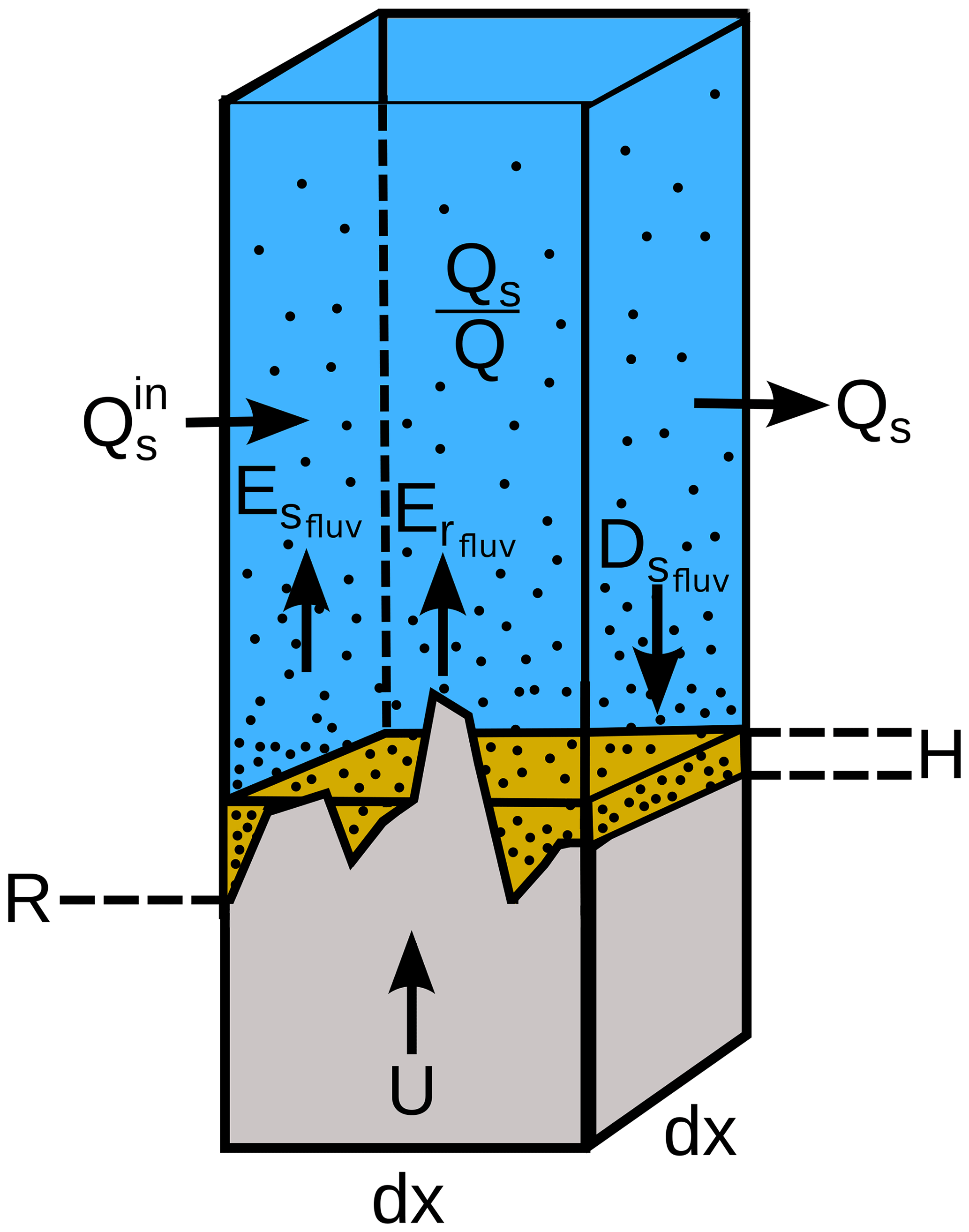
Figure 1 Sketch of fluvial SPACE component. Model setup and variable definitions for the SPACE bedrock–alluvial river erosion model. Entrainment and deposition of sediment, as well as erosion of bedrock, can occur simultaneously. This approach allows channels to dynamically transition among bedrock, bedrock–alluvial and fully alluviated states. At a given stream power, the relative rates of sediment entrainment $E_{{\mathrm{s}}_{\text{fluv}}}$ and bedrock erosion $E_{{\mathrm{r}}_{\text{fluv}}}$ are set by the ratio of sediment thickness H to the bedrock roughness height H_* (Fig. 2). Modified from Shobe et al. (2017).

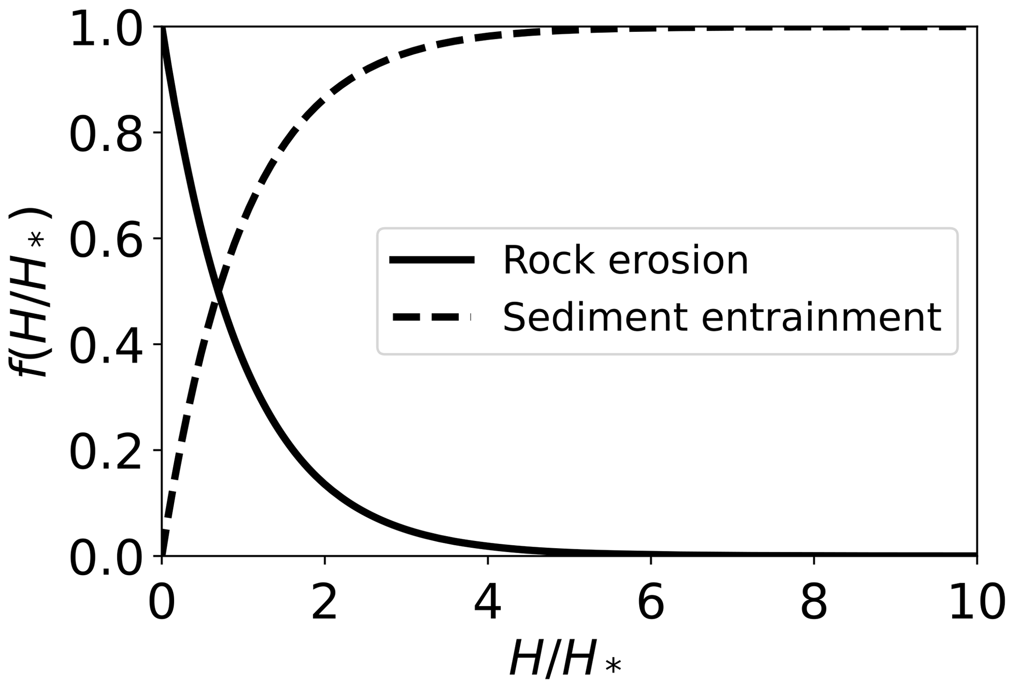
Figure 2 Relative efficiency of fluvial sediment entrainment and bedrock erosion, $f\left(H/H_{*}\right)$, as a function of the ratio of sediment thickness to bedrock roughness $H/H_{*}$. $f\left(H/H_{*}\right)$ depends only on the ratio $H/H_{*}$, varies between 0 and 1, and indicates the proportion of total stream power used to entrain sediment – see Eq. 3; $f\left(H/H_{*}\right)=\mathrm{1}-e^{-H/H_{*}}$ (dashed line) – or erode bedrock – see Eq. 4; $f\left(H/H_{*}\right)=e^{-H/H_{*}}$ (solid line). As sediment thickness H increases relative to the bedrock roughness length scale H_*, the sediment entrainment rate factor approaches 1 and the bedrock erosion rate factor approaches 0 because the bed becomes composed entirely of sediment, and no bedrock is exposed. As sediment thickness declines relative to the bedrock roughness length scale, the bedrock erosion rate increases exponentially because more bedrock is exposed, and the sediment entrainment rate declines exponentially due to a lack of available sediment. This approach implements the “cover effect”, in which the presence of sediment reduces bedrock erosion rates but does not incorporate the “tools effect”, in which mobile sediment enhances bedrock erosion. Modified from Shobe et al. (2017).

2.2 Landsliding

HyLands treats landslide erosion and deposition deterministically but uses a stochastic approach to calculating landslide occurrence. HyLands simulates deep-seated gravitational landslides eroding simultaneously the sediment layer and the bedrock (erosion terms $E_{{\mathrm{s}}_{\text{hill}}}$ and $E_{{\mathrm{r}}_{\text{hill}}}$, respectively, in Eq. 1). We assume that both the rock and the sediment layer behave as Mohr–Coulomb materials. In its current form, HyLands does not simulate shallow landslides where failure geometry is imposed by the depth and angle of soil–rock transitions. Landslide initiation does not involve a preceding triggering event (e.g., an earthquake) but is simulated using a probabilistic approach.

2.2.1 Landslide erosion

Following Densmore et al. (1998), we simulate landslide erosion using the Culmann theory for slope stability. Culmann (1875) proposes that hillslope failure will occur on the plane where the shear stress is balanced by the sliding resistance. Assuming Mohr–Coulomb materials, it has been shown that the failure plane with a dip θ_c bisects the local topographic slope β and the material's angle of internal friction ϕ (Densmore et al., 1998; Champel, 2002) as follows:

$$\begin{array}{}\text{(6)}& {\mathit{\theta }}_{\mathrm{c}}={\displaystyle \frac{\mathit{\beta }+\mathit{\varphi }}{\mathrm{2}}}.\end{array}$$

Note that Eq. (6) implies that failure occurs at angles higher than ϕ, being the consequence of the force balance controlled by material properties (Eq. 8) and the mass of the wedge above the failure plane (Culmann, 1875). The implementation of the Culmann theory in HyLands is illustrated in Fig. 3. For all points within the landscape where a landslide is initialized, the failure plane dipping at θ_c is extended until it daylights (i.e., intersects the topographic surface).

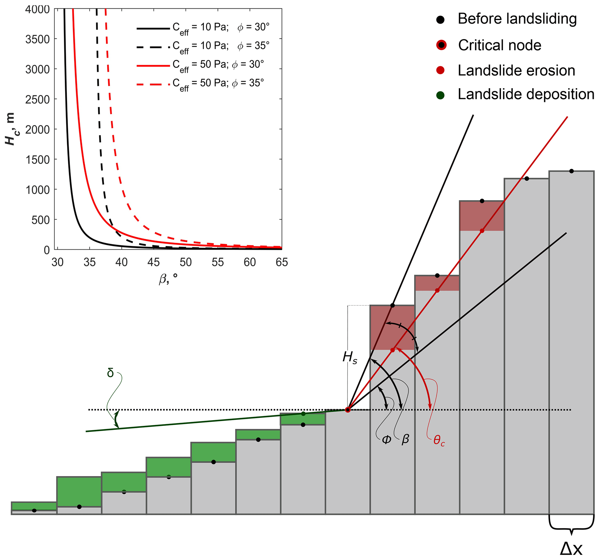
Figure 3 Sketch of landslide algorithm in two dimensions. Landslide erosion (red shaded area) is calculated using the Culmann approach (Culmann, 1875). β is the topographic slope; ϕ represents the angle of internal friction, and θ is the inclination of the rupture plane. Deposition of landslide-derived sediment (green shaded area) is calculated using a nonlocal diffusion equation (Eq. 11; see Carretier et al., 2016). δ is the minimal deposit surface angle at which landslide-derived sediment is distributed on the hillslope. This sketch illustrates a case where none of the landslide-derived sediment is in permanent suspension $(F_{{\mathrm{f}}_{\text{hill}}}=\mathrm{0})$ and the amount of eroded sediment (red shaded area) equals the amount of deposited sediment (green shaded area). If the deposited volume creates a downslope gradient which is lower than δ, the slope of the deposited volume is adjusted so that the deposit surface angle equals δ. Probability for sliding is calculated as the ratio of the local hillslope height H_s to the maximum hillslope height H_c (Eq. 7; see Densmore et al., 1998). The inset plot illustrates that H_c depends on the rock strength (cohesion C and internal friction angle ϕ) and the topographic slope β. The plotted lines are calculated using Eq. 8, where ρ is 2700 kg m⁻³ and g = 9.81 m s⁻².

Modeling landslide frequency and location depends critically on the identification of points in the landscape where landslides initiate. A wide variety of events ranging from coseismic activity and peak ground acceleration (Meunier et al., 2007) over intense storm events (Marc et al., 2018) to human hillslope destabilization (Guns and Vanacker, 2014) may trigger mass wasting through landslide activity. Although these triggers could be added, HyLands mainly aims to simulate the impact of topographic landscape configuration on landslide activity. Therefore, we follow Densmore et al. (1998) in identifying unstable grid cells as points in the landscape where the topographic slope (β) exceeds the angle of internal friction (ϕ). For all unstable cells, the probability for sliding, p_LS, is calculated as

$$\begin{array}{}\text{(7)}& p_{\mathrm{LS}}={\displaystyle \frac{H_{\mathrm{s}}}{H_{\mathrm{c}}}},\end{array}$$

where H_s is the local hillslope height calculated as difference between every cell in the landscape and its highest neighbor (Fig. 3), and H_c is the maximum stable hillslope height, which is calculated as (Densmore et al., 1998; Champel, 2002)

$$\begin{array}{}\text{(8)}& {\displaystyle }{H}_{\mathrm{c}}{\displaystyle }={\displaystyle \frac{\mathrm{4}C}{\mathit{\rho }g}}{\displaystyle \frac{\sin \mathit{\beta }\cos \mathit{\varphi }}{\mathrm{1}-\cos (\mathit{\beta }-\mathit{\varphi })}}.\end{array}$$

Here C is the cohesion (M L⁻¹ T⁻²), ρ is the rock density (M L⁻³) set to 2700 kg m⁻³, and g is the gravitational acceleration (g=9.81 ms⁻²). To simulate the random nature of landslides, grid cells where landslides initiate are selected using a stochastic sampling scheme:

$$\begin{array}{}\text{(9)}& r{\displaystyle \frac{\mathrm{d}t}{t_{\mathrm{LS}}}}\left\{\begin{array}{ll}>p_{\mathrm{LS}}& \text{No landsliding}\\ <p_{\mathrm{LS}}& \text{Landsliding, select as critical cell, }\end{array}\right.\end{array}$$

where r is a random number between 0 and 1, and t_LS is the return time for landslides with t_LS>=dt, where dt is the model time step. Unstable cells where a landslide is induced will further be referred to as critical cells (Fig. 3). At every model iteration, Eq. (9) is updated for all cells where the topographic gradient (β) exceeds the critical material friction angle (ϕ). From Eqs. (8) and (9), it follows that the probability for sliding depends on the topographic slope, β, and inversely correlates with the angle of internal friction, ϕ, and the cohesion of the material, C (see inset of Fig. 3). Cohesion is a scale-dependent variable, and parameter values covering several orders of magnitude have been reported (Sidle and Ochiai, 2006). Jeandet et al. (2019) inverted several landslide inventories and found effective cohesion values ranging between 10 and 35 kPa. These values are lower than geomechanical values representing large-scale rock strength (e.g., Densmore et al., 1998; Champel, 2002), which is attributed to the decrease in rock cohesion in the vicinity of faults following earthquakes (Gallen et al., 2015). In our experiments, we will use values for cohesion in the range reported by Jeandet et al. (2019), which represent effective cohesion following an earthquake or a storm.

The landslide return time t_LS controls the absolute number of critical cells where landslides are initiated. If t_LS equals the time step dt, the number of landslides per time step is solely controlled by the ratio H_s∕H_c. When $t_{\mathrm{LS}}\gg H_{\mathrm{s}}/H_{\mathrm{c}}$, however, the number of landslides per time step is reduced (Eq. 9). While the H_s∕H_c ratio controls the topographic location of landsliding onset and thus the landslide characteristics (size and volume), the landslide return time t_LS controls the absolute number of landslides and therefore overall landslide erosion rates.

HyLands enables the simulation of landslides at every location in the landscape. At every iteration, landslides are induced at critical cells sampled using the probabilistic approach outlined above (Eq. 9, Figs. 3 and 4). We propose a recursive approach to calculate the magnitude of a single landslide. For every critical cell, we build a stack of unstable (i.e., sliding) cells. The stack is initialized by adding the critical cell. Next, a recursive procedure is applied until the stack is empty. This procedure consists of the following steps: (i) select the first cell from the stack (thus starting with the critical cell). (ii) Evaluate all up-slope neighboring cells. If the elevation of a neighboring cell exceeds the elevation of the sliding plane defined by θ_c, the cell is identified as a sliding cell and added the to stack of landslide cells. (iii) Remove the first cell from the stack. This procedure is repeated until the stack is empty. HyLands offers the possibility to set a maximum landslide area $\left(A_{{\mathrm{LS}}_{\max }}\right)$. Once this maximum is achieved – or when no more cells are added to the stack of landslide cells – the landslide area is defined. All cells inside this area are eroded to the elevation of the sliding plane, thereby adjusting both $E_{{\mathrm{s}}_{\text{hill}}}$ and $E_{{\mathrm{r}}_{\text{hill}}}$ of Eq. (1) for all cells involved.

2.2.2 Hillslope-derived sediment

The spatial change in hillslope-derived volumetric sediment discharge $Q_{{\mathrm{s}}_{\text{hill}}}$ (L³ T⁻¹) per unit width w (L) is written as

$$\begin{array}{}\text{(10)}& {\displaystyle \frac{\partial \left(Q_{{\mathrm{s}}_{\text{Hill}}}/w\right)}{\partial x}}=E_{{\mathrm{s}}_{\text{hill}}}+\left(\mathrm{1}-F_{{\mathrm{f}}_{\text{hill}}}\right)E_{{\mathrm{r}}_{\text{hill}}}-D_{{\mathrm{s}}_{\text{hill}}},\end{array}$$

where $F_{{\mathrm{f}}_{\text{hill}}}$ is a unitless fraction of fine hillslope-derived sediment. The factor $\mathrm{1}-F_{{\mathrm{f}}_{\text{hill}}}$ (–) represents the idea that some fraction of the hillslope-derived sediment is rapidly evacuated in high suspension (Page et al., 1999; Hovius et al., 2000; Lin et al., 2008; Tenorio et al., 2018) and therefore should not be tracked as sediment. When $F_{{\mathrm{f}}_{\text{hill}}}=\mathrm{0}$, the system is fully mass conservative, and all sediments produced by landslide activity contribute to the sediment discharge (Eq. 1). Note that both $E_{{\mathrm{s}}_{\text{hill}}}$ and $D_{{\mathrm{s}}_{\text{hill}}}$ are corrected for dimensionless sediment porosity (ϕ_sed in Eq. 1), thereby factoring in the increase in bedrock-derived landslide sediment volumes during deposition due to the addition of pore spaces.

2.2.3 Deposition of landslide material

In the following we describe how deposition of landslide-derived material is being calculated. In HyLands, landslides can initiate at any point in the landscape (Fig. 4). A steepest-descent flow routing algorithm is known to be unrealistic for flow and sediment redistribution on hillslopes (Pelletier, 2010). Moreover, the use a constant spreading slope, as suggested by Densmore et al. (1998), does not take into account the topographic relief when redistributing landslide-derived sediment. When using a constant sediment spreading slope, sediment deposited on flat parts of the landscape is spread out over much longer distances than sediment deposited on steep parts. This is not realistic, as sediment travel distance should depend on topographic gradient: material traveling over steeper slopes should go farther, all else being equal (Roering et al., 1999; Campforts et al., 2016).

A common approach to simulate sediment transport and deposition on hillslopes while considering the topographic gradient is the use of linear or nonlinear diffusion equations (Roering et al., 1999; Andrews and Hanks, 1985). However, such an approach is not suited to simulate the distribution of landslide-derived sediment. While diffusion equations distribute sediment only between the neighboring cells of a cell, landslide-derived sediment has run-out distances that can be significantly longer than a single grid cell (Claessens et al., 2007). Therefore, we adopt a nonlinear, nonlocal deposition scheme for landslide-derived sediment outlined by Carretier et al. (2016):

$$\begin{array}{}\text{(11)}& D_{{\mathrm{s}}_{\text{hill}}}={\displaystyle \frac{Q_{{\mathrm{s}}_{\text{Hill}}}/w}{L}},\end{array}$$

where $D_{{\mathrm{s}}_{\text{hill}}}$ (L T⁻¹) is the volumetric deposition flux of hillslope-derived sediment per unit bed area and L (L) represents a sediment transport distance. The larger the L, the bigger the distance over which sediments are transported and the lower the local deposition rate. L is calculated for every grid cell as follows:

$$\begin{array}{}\text{(12)}& L={\displaystyle \frac{\mathrm{d}x}{\mathrm{1}-{\left(\frac{S}{S_{\mathrm{c}}}\right)}^{\mathrm{2}}}},\end{array}$$

where S_c is a critical slope which we further assume to be equal to the angle of internal friction (ϕ). When the hillslope gradient S≪S_c, most of the incoming sediment will be deposited, and the resulting outcome is similar to the one obtained using a regular diffusion equation, also referred to as a local solution (Furbish and Roering, 2013; Carretier et al., 2016). When S approaches S_c, L goes to infinity implying that no deposition will occur at the considered cell. At steep slopes, sediment transport therefore shows nonlocal behavior in the sense that erosion of nonlocal, upstream cells is integrated when calculating the sediment discharge Q_s (Carretier et al., 2016). When S>S_c, L is set to ∞, and there is no deposition at that cell. For negative values of S, which might occur for flooded cells, L is set to dx. A minimal angle (δ) under which landslide-derived sediments should be deposited can be set as a parameter value but is not required to run HyLands (Fig. 3).

Contrary to the fluvial component of the model (SPACE) where a single flow direction algorithm (steepest descent) is used, landslide-derived sediment is spread over the landscape using a multiple-flow-direction algorithm redistributing sediment over the downstream cells in proportion to the local slope (Fig. 4; see Carretier et al., 2016). When a lot of sediment is debouched into fluvial channels, rivers can be blocked by landslide dams. HyLands uses a lake identification algorithm to identify flooded cells during every model iteration. Lakes are identified by filling all sinks in a landscape to the brim (Schwanghart and Scherler, 2014). By default, flooded cells do not erode but do allow for sediment deposition (Eq. 5). HyLands enables spatially variable values for V (Eq. 5) to distinguish between settling velocities in non-flooded versus flooded cells by changing the values for V and V_Lake, respectively (see Table 1).

In the remainder of this paper, we will first evaluate the performance of the fluvial and landslide components of HyLands through a set of verification and validation runs. Next, the coupling between landslide activity and long-term landscape evolution will be evaluated using a synthetic model setup where a steady-state landscape is exposed to a pulse of landslides. All model experiments executed in the framework of this paper are available as executable MATLAB scripts and as dynamic landscape evolution movies (Table 2).

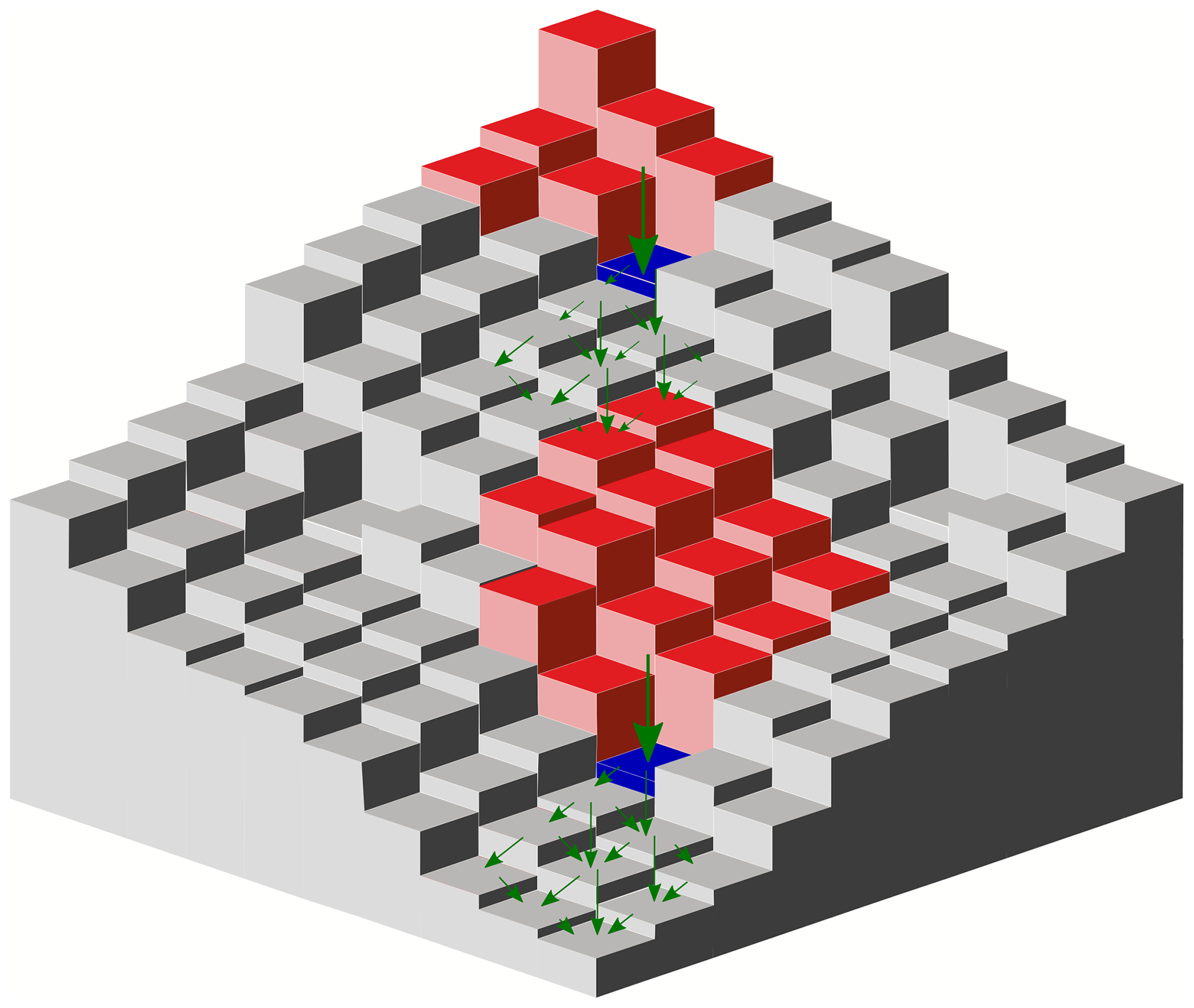
Figure 4 Sketch of landslide algorithm in three dimensions. Cells shaded in blue indicate the critical cells where landslides potentially initiate. Cells shaded in red represent the landslide source areas. After mass failing, sediment will be redistributed over the downslope cells using a multiple-flow-direction algorithm (indicated with green arrows). Sediment deposition rate depends on a transport distance L (see Eqs. 11 and 12).

3 Verification and evaluation

3.1 Comparison to analytical solutions for the fluvial component

In the first three test runs (detachment-limited, transport-limited and mixed), a steady-state artificial landscape is simulated using a square grid of 20 by 20 cells with a spatial resolution of 100 m. The landsliding component is turned off for these runs (i.e., only fluvial erosion according to the SPACE model occurs). Each run is initialized from a surface with randomly generated microtopography. The initial surface is a tilted plane which drains towards the southwestern corner, the only open boundary cell. Therefore sediment and water can only leave the domain through this southwestern corner. The setup is identical to the one proposed by Shobe et al. (2017) in order to facilitate comparison. The time step is set to 10 years. Under detachment-limited conditions (imposed by setting F_f=1), the sediment thickness H equals 0 everywhere through the entire model run and sediment produced by river incision into bedrock is instantaneously evacuated from the simulated domain. When assuming that water discharge is proportional to the drainage area (q∝A^m) it has been shown that fluvial erosion results in the following steady-state slope–area relationship (Shobe et al., 2017):

$$\begin{array}{}\text{(13)}& S={\left({\displaystyle \frac{U}{K_{\mathrm{r}}{A}^m}}\right)}^{\mathrm{1}/n}.\end{array}$$

Figure 5b illustrates that when using parameter values listed in Table 1, HyLands reproduces the slope–area relationship given by Eq. (13). Similarly, it can be shown that under transport-limited conditions where $H\gg H_{*}$, the theoretical slope–area relationship for fluvial incision can be written as (Shobe et al., 2017)

$$\begin{array}{}\text{(14)}& S={\left[{\displaystyle \frac{V}{r}}+\mathrm{1}\right]}^{\mathrm{1}/n}{\left[{\displaystyle \frac{U}{K_{\mathrm{s}}}}\right]}^{\mathrm{1}/n}{A}^{-m/n},\end{array}$$

where r represents the runoff rate (L T⁻¹). To mimic a transport-limited configuration, we run HyLands assigning an initial sediment thickness H of 100 m. Other parameters values are shown in Table 1. Figure 5d illustrates the slope–area plot for all cells of the simulated steady-state landscape showing a close match with the analytical prediction (14). Moreover, HyLands also reproduces the theoretical steady-state sediment discharge relationship for transport-limited conditions with $F_{{\mathrm{f}}_{\text{fluv}}}=\mathrm{0}$ (Shobe et al., 2017):

$$\begin{array}{}\text{(15)}& Q_{{\mathrm{s}}_{\text{fluv}}}=UA.\end{array}$$

Finally, we evaluate the hybrid nature of the SPACE component in simultaneously simulating fluvial bedrock incision and sediment dynamics. Under such conditions the slope–area relationship can be written as (Shobe et al., 2017)

$$\begin{array}{}\text{(16)}& S={\left[{\displaystyle \frac{UV}{K_{\mathrm{s}}{A}^{m}r}}+{\displaystyle \frac{U}{K_{\mathrm{r}}{A}^m}}\right]}^{\mathrm{1}/n}.\end{array}$$

At steady state, both the height of the bedrock and the sediment layer should remain unchanged so that

$$\begin{array}{}\text{(17)}& {\displaystyle \frac{\partial \mathit{\eta }}{\partial t}}={\displaystyle \frac{\partial R}{\partial t}}+{\displaystyle \frac{\partial H}{\partial t}}=\mathrm{0}+\mathrm{0}=\mathrm{0},\end{array}$$

which leads to a constant soil thickness over the landscape derived by (Shobe et al., 2017)

$$\begin{array}{}\text{(18)}& H=-H_{*}\ln \left[\mathrm{1}-{\displaystyle \frac{V}{\frac{K_{\mathrm{s}}r}{K_{\mathrm{r}}}+V}}\right].\end{array}$$

To evaluate the performance of the hybrid fluvial dynamics, we run HyLands to a steady state, starting from an initial surface without any sediment cover and using parameter values listed in Table 1. The obtained slope–area relationship (Fig. 5g) matches the theoretical relationship in Eq. (16) and so does the soil thickness H, which evolves toward a constant thickness (Eq. 18), and Q_s, adhering to the sediment discharge relationship (Eq. 15).

Table 1 Parameter values.

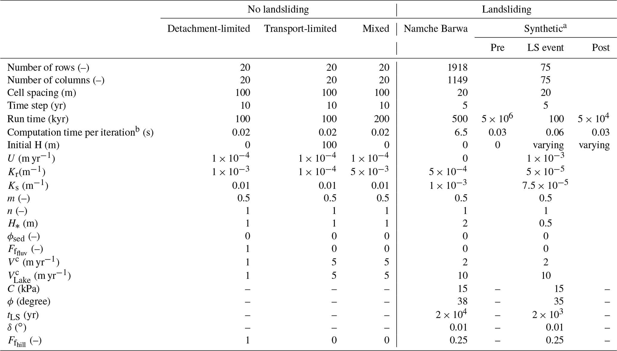
Not all parameters will influence the model outcome in all cases. For example, the value of V is irrelevant for the detachment-limited case when all eroded bedrock passes out of the model domain as permanently suspended fine sediment $(F_{{\mathrm{f}}_{\text{fluv}}}=\mathrm{1})$. Landslide parameters are only relevant for models where landslide activity is simulated. ^a The synthetic landscape evolution model consists of three stages: a pre-landslide stage, a landslide stage and a post-landslide stage. Only parameter values which differ for these stages are listed in the table. ^b Time spent to complete one full model iteration on a Windows PC, with an Intel® Core^™ i9-9880H CPU at 2.30 GHz and a RAM of 32 GB. ^c HyLands enables spatially variable values for V (Eq. 5) to distinguish between settling velocities in non-flooded versus flooded cells by changing the values for V and V_Lake, respectively.

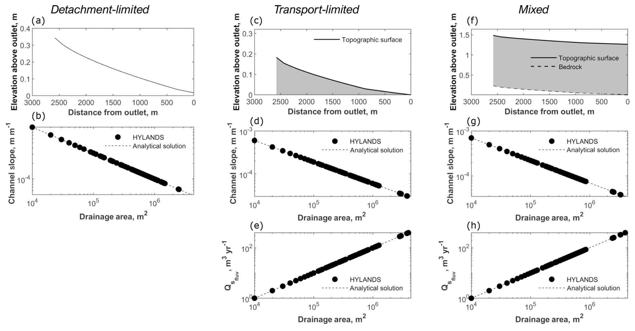
Figure 5 Verification of fluvial SPACE component. (a) Longitudinal profile of the trunk stream at steady state under detachment-limited conditions where no sediment is present because $F_{{\mathrm{f}}_{\text{fluv}}}=\mathrm{1}$, and all produced sediment is assumed to be evacuated instantaneously. At steady state, the concave-upward profile is in equilibrium with the imposed rock uplift pattern. The steady-state slope–area relationship (b) matches the analytical solution (Eq. 13). (c) Longitudinal profile of the trunk stream at steady state under transport-limited conditions. At steady state, the concave-upward profile is in equilibrium with the imposed rock uplift pattern. The steady-state slope–area relationship (d) matches the analytical solution (Eq. 14). Panel (e) illustrates the steady-state fluvial sediment discharge $\left(Q_{{\mathrm{s}}_{\mathrm{fluv}}}\right)$ as a function of the drainage area, which matches the analytical area–sediment discharge relationship (Eq. 15). (f) Longitudinal profile of the trunk stream at steady state under mixed bedrock–alluvial conditions. At steady state, both the topographic and bedrock profiles are in equilibrium with the imposed rock uplift pattern. The steady-state slope–area relationship (g) matches the analytical solution (Eq. 16). Panel (h) illustrates the steady-state fluvial sediment discharge $\left(Q_{{\mathrm{s}}_{\mathrm{fluv}}}\right)$ as a function of the drainage area, which matches the analytical area–sediment discharge relationship (Eq. 15).

3.2 Evaluation of the landslide component

Because landsliding is a stochastic process, it is not possible to derive an exact, analytical, solution to evaluate the performance of the landslide component in HyLands. However, it has been shown that most landslide inventories obey consistent magnitude–frequency and magnitude–volume relationships (Malamud and Turcotte, 1999; Stark and Hovius, 2001; Guzzetti et al., 2002; Korup, 2005; Guns and Vanacker, 2014; Larsen and Montgomery, 2012). To evaluate the performance of HyLands, we run the model over a limited amount of time for an area where both relationships are well constrained. The performance of the landslide module is evaluated based on its capacity to reproduce those calibrated relationships.

3.2.1 Landslide scaling relationships

A first empirical universal relationship is the landslide magnitude–frequency distribution that describes the number of landslide events of a given size. This relationship is characterized by a negative power law for landslides having an area greater than a given threshold value and a characteristic rollover for smaller landslides (Stark and Hovius, 2001; Malamud and Turcotte, 1999; Guzzetti et al., 2002). Magnitude–frequency distributions are typically described using a three-parameter inverse gamma distribution as (Malamud et al., 2004)

$$\begin{array}{}\text{(19)}& \begin{array}{rl}p(A_{\mathrm{L}};{\mathit{\rho }}_l,a_l,s_l)=& {\displaystyle \frac{\mathrm{1}}{a_l\mathrm{\Gamma }\left({\mathit{\rho }}_l\right)}}{\left[{\displaystyle \frac{a_l}{A_{\mathrm{L}}-s_l}}\right]}^{{\mathit{\rho }}_l+\mathrm{1}}\\ & \exp \left[-{\displaystyle \frac{a_l}{A_{\mathrm{L}}-s_l}}\right],\end{array}\end{array}$$

where A_L is the landslide area (L²), p(A_L) is the probability density of a landslide area (A_L), a_l, s_l, and ρ_l are empirical parameters, and Γ(ρ_l) is the gamma function of ρ_l. A second empirical universal relationship is the volume–area scaling relationship where the volume V_L of a given landslide is a function of its area A_L as (Hovius et al., 1997)

$$\begin{array}{}\text{(20)}& V_{\mathrm{L}}={\mathit{\alpha }}_l{A}_{\mathrm{L}}^{{\mathit{\gamma }}_l},\end{array}$$

where α_l is an intercept and γ_l a scaling exponent.

3.2.2 Applying HyLands to the Namche Barwa–Gyala Peri massif

To evaluate to the performance of HyLands, the model is applied to a digital elevation model (DEM) of the Eastern Himalaya where the Yarlung Tsangpo river cuts through the Namche Barwa–Gyala Peri massif (Fig. 6). The area is characterized by rapid exhumation (King et al., 2016), steep topography and steep river gradients causing high stream power (Finnegan et al., 2008). To quantify erosion rates in the area, Larsen and Montgomery (2012) mapped more than 15 000 landslides and constructed an inventory of landslides predating 1974 and an inventory containing all landslide events between 1974 and 2007 (Fig. 8a). We use this area solely to demonstrate and evaluate the performance of HyLands and do not aim to reproduce exact features of landscape exhumation in this region. We selected the Namche Barwa–Gyala Peri massif to evaluate the performance of HyLands given its unique geomorphologic configuration featuring amongst the highest globally documented river stream power in combination with very active hillslope processes (Larsen and Montgomery, 2012). With HyLands being designed to couple the role of fluvial and hillslope processes, this region makes for a good test environment. Note however that we do not intend to calibrate nor validate the model but run it using fixed, theoretical model parameters (Sect. 3.2.3). Applications of HyLands aiming to constrain the model through parameter calibration and validation (Sect. 4.3) would require additional data to ground-truth landslide inventories and to provide detailed records on landslide triggers such as earthquakes and storms.

Figure 6 Namche Barwa–Gyala Peri massif used for model evaluation. The red rectangle on the inset figure indicates the location of the study area. The green dashed rectangle indicates the part of the DEM used to evaluate HyLands. The shaded colors show elevation derived from the 30 m SRTM v3 DEM (Farr et al., 2007) and resampled to a higher resolution of 20 m using a bicubic interpolation method. Main map is produced with TopoToolbox (Schwanghart and Scherler, 2014). Inset map is made in QGIS 3.10.9, using Natural Earth vector and raster map data available at http://www.naturalearthdata.com (last access: 25 August 2020).

3.2.3 Model parameterization

We run HyLands using the NASA Shuttle Radar Topography Mission (SRTM) v3.0 elevation dataset as an initial surface (Farr et al., 2007), resampled to a higher resolution of 20 m using a bicubic interpolation method. We resampled the DEM to a resolution of 20 m in order to evaluate the capacity of HyLands to reproduce the rollover in the magnitude frequency distribution, often reported to occur for landslide areas <900 m², which would be the minimum landslide area when using the original SRTM data. As shown in Fig. 6, we only simulate part of the larger Namche Barwa–Gyala Peri massif studied by Larsen and Montgomery (2012). We selected a region mostly free of glaciers and surrounding the section of the Yarlung Tsangpo river where unit stream power is very high (ranging between 500 and 4000 W m²; Finnegan et al., 2008. The simulated grid is composed of 1918×1149 cells, covering a total area of ca. 960 km². We simulate landscape evolution over 500 years, using time steps of 5 years. For this experimental run, we assume that there is no uplift. We acknowledge that this condition is not met in the area, but imposing an uplift field is not necessary for evaluating the performance of the HyLands landsliding algorithm. Inserting realistic uplift patterns to simulate the dynamic evolution of the area would require (i) implementation of the complex tectonic configuration of the area (King et al., 2016) and (ii) simulation of a bigger area to capture the dynamic interplay between uplift and river dynamics. This is beyond the scope of the application, and we therefore assume that the tectonic configuration controlling landscape evolution over the limited timescale simulated in this experiment (500 years) is captured by the topography of the area (Kirby and Whipple, 2012).

We run HyLands assuming open boundary conditions: all sediment produced within the domain through river incision and landsliding can be exported from the domain across any of the four boundaries. For simplicity, we use a simple stream power formulation for river incision where thresholds for both sediment entrainment and bedrock erosion are negligible. Standard scaling exponents are used (m=0.5 and n=1 in Eq. 4), and the bed sediment porosity and the fraction of fine river sediments are assumed to be zero (ϕ_sed=0 and $F_{{\mathrm{f}}_{\text{fluv}}}=\mathrm{0}$ in Eq. 1). We calculate landslide activity using the landslide module of HyLands and assume that 25 % of the landslide-derived sediment is evacuated out of the system as fine material ($F_{{\mathrm{f}}_{\text{hill}}}=\mathrm{0.25}$). We assume that the angle of internal friction (ϕ) is comparable to the mode of the topographical slope distribution (Burbank et al., 1996; Korup, 2008; Montgomery and Gran, 2001), reported to range between 37 and 39^∘ and here set to 38^∘ (Larsen and Montgomery, 2012). Cohesion C is known to vary over a wide range and strongly depends on rock mechanical properties (Wyllie and Mah, 2017). Site-specific calibration would require detailed mapping of lithological units, and we therefore set C to 15 kPa, a value in the range of previously optimized cohesion for the Himalaya (12–20 Pa in Jeandet et al., 2019). Cohesion and the angle of internal friction influence the size distribution of landslides in several ways (Jeandet et al., 2019). The angle of internal friction ϕ controls the angle of the potential rupture plane such that lower values of ϕ will result in lower rupture dipping angles, which, for the same topographical configuration, results in thicker and larger landslides. The effective rock cohesion value C influences the critical hillslope height H_c in Eq. (6). Larger values for C will result in larger values for H_c, thus decreasing the probability of landslides on gentler slopes and resulting in fewer small landslides. The minimum value of the minimal deposit surface angle under which landslide-derived sediment is redistributed on hillslopes is set to 0.01^∘. We set the return time for landsliding t_LS to 2×10⁴ years. t_LS regulates the probability that unstable cells evolve into a landslide (Eq. 9) and therefore controls the number of landslide events per time step Δt. When applying HyLands to reconstruct or predict landslide activity, t_LS should be a function of the frequency (or return time) of triggering events (large earthquakes or rainfall events). Evaluation of model sensitivity to changing values for t_LS is a natural avenue for further work. A full overview of the model parameters is given in Table 1.

(Campforts, 2020b)(Campforts, 2020c)(Campforts, 2020d)(Campforts, 2020e)(Campforts, 2020f)(Campforts, 2020g)(Campforts, 2020h)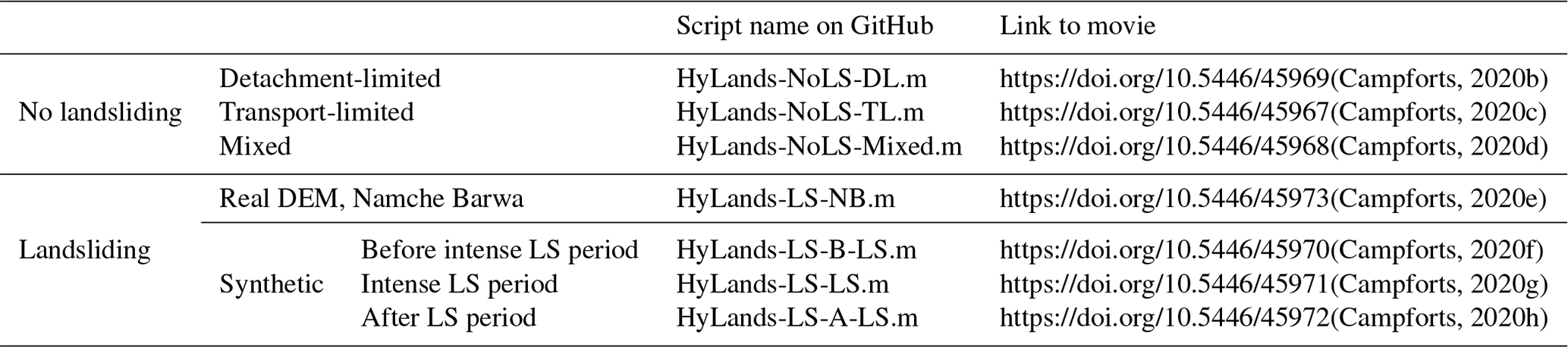

Table 2 Simulation movies and script names.

Figure 7 Time slices of HyLands model run for the Namche Barwa–Gyala Peri massif after 5, 165, 330 and 500 model years. Panels (a), (d), (g) and (j) indicate the location of the landslides at the given time step (black diamonds). Panels (b), (e), (h) and (k) zoom into the red squares in (a), (d), (g) and (j) showing simulated landslide erosion–deposition. The colors represent the square root (for ease of visualization) of landslide erosion (−) and deposition (+) during the presented time step. Panels (c), (f), (i) and (l) show the sediment thickness, H, generated through river incision (SPACE module) and landsliding. The underlying hillshade was derived from the 30 m SRTM v3 DEM (Farr et al., 2007).

3.2.4 Model evaluation results

Figure 7 shows time slices of the model run after 5 (initial iteration), 165, 330 and 500 (final iteration) model years. Locations for landslide initiation (critical cells) are well spread over the landscape. The number of landslide events (the number of black diamonds in Fig. 7) is mainly controlled by the return time for landsliding t_LS. The fan-shaped deposition zones of landslide-derived sediments reflect the use of a multiple-flow sediment routing algorithm. Landslide-derived sediment predominantly accumulates at hillslope toes, as well as in or near river channels. Some accumulation also occurs on hillslopes. Overall, landslides strongly influence the thickness of the alluvial bed sediment layer. Note that the shape of the erosion and deposition zones adjust through the course of the model run. The presence of previous landslide activity alters the topographic relief and hence determines which cells become susceptible to erosion and deposition as landscape evolution continues (e.g., the deposition pattern in Fig. 7h reflects the shape of erosion patterns resulting from previous landslide activity).

To quantitatively evaluate the performance of the HyLands landslide module, we compare modeled landslide properties against observed scaling relationships (Eqs. 19 and 20). Figure 8a compares the modeled and observed magnitude–frequency distribution. We observe good correspondence between the model and the data, with the power-law tail of the distribution falling within the envelope defined by the two inventories of Larsen and Montgomery (2012). Similarly to observed magnitude–frequency distributions, HyLands simulates the rollover or the transition from an increasing magnitude–frequency relationship to a decreasing one. This observation confirms that the shape of landslide magnitude–frequency distributions can be explained using mechanical landslide processes (see Sect. 2.2.1) and the topography of the studied region (Jeandet et al., 2019). Figure 8b shows that HyLands is capable of approaching the shape of the universal area–volume relationships found by Larsen et al. (2010). While HyLands seems to overestimate simulated landslide volumes for very small landslides, the area–volume relationship simulated with HyLands approaches a linear relationship in a log–log space for larger landslides, similar to the shape of the observed area–volume relationship. Note that overall, landslide volumes simulated with HyLands are overpredicted compared to observations. Study-area-specific model calibration would improve this fit but is beyond the scope of this model evaluation in which we evaluate the capacity of HyLands to reproduce the shape of the universal area–volume relationship. We attribute the positive deviation from the linear area–volume relationship in a log–log space for smaller landslides to the nature of the landslide algorithm. HyLands simulates deep-seated landslides; several of the smaller landslides are likely to be shallow landslides, which are currently not simulated. Moreover, HyLands does not allow any sediment to be deposited within the landslide scar, while this typically does occur in nature. Future developments of the algorithm could allow for shallow landsliding and in-scar deposition for more realistic simulations. Furthermore, there is a resolution effect: due to DEM noise or heterogeneity, the algorithm might select small landslides of one or two cells on very steep hillslope patches, thus resulting in high landslide volumes. However, such steep hillslope patches might represent noise in the DEM rather than actual steep slopes.

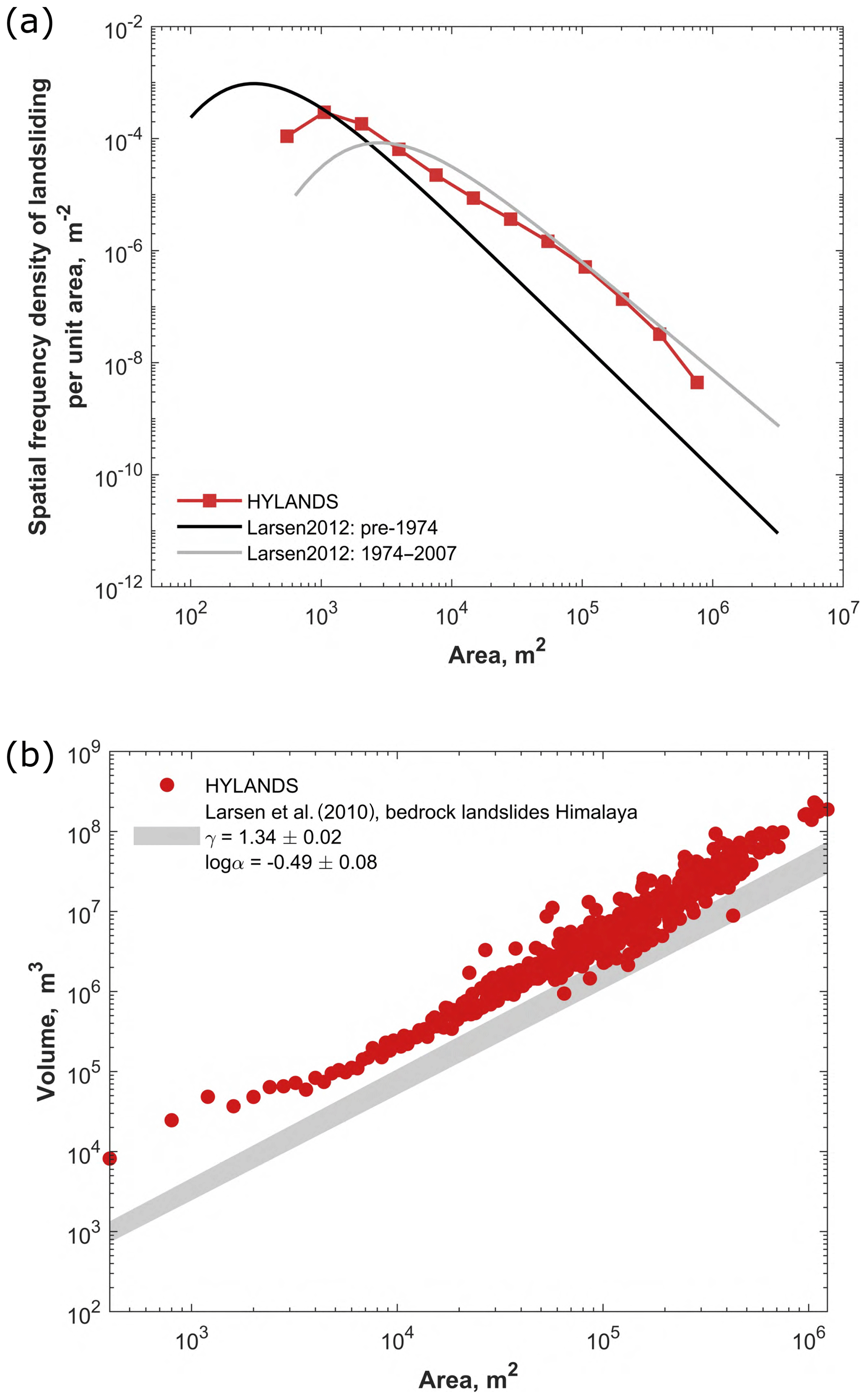
Figure 8 Comparison between modeled and observed characteristic landslide scaling relationships. (a) Magnitude–frequency relationship. The grey and black lines represent the best-fitting inverse gamma distribution (Eq. 19) of the landslide activity mapped before 1974 and between 1974 and 2012, respectively (Larsen and Montgomery, 2012). The fitting parameters are, respectively, ($a_l=\mathrm{768}\times {\mathrm{10}}^{-\mathrm{6}}$, $s_l=-\mathrm{32.6}\times {\mathrm{10}}^{-\mathrm{6}}$, ρ_l=1.27) and ($a_l=\mathrm{6100}\times {\mathrm{10}}^{-\mathrm{6}}$, $s_l=-\mathrm{311}\times {\mathrm{10}}^{-\mathrm{6}}$, ρ_l=0.96). The red dots represent the magnitude–frequency distribution simulated using HyLands. (b) Area–volume relationship. The grey dashed zone represents the expected area–volume scaling relationship, observed for bedrock landslides in the Himalaya (Larsen et al., 2010). Fit is calculated using Eq. (20) with fitting parameters $\mathit{\gamma }=\mathrm{1.32}\pm \mathrm{0.02}$ and ${}^{\mathrm{10}}\log \mathit{\alpha }=-\mathrm{0.49}\pm \mathrm{0.06}$. The red dots represent the geometry of the landslides simulated with HyLands.

3.3 Model application

The explicit coupling of landslides and landslide-derived sediment to long-term landscape evolution enables the study of a wide range of interactions which otherwise can only be inferred or partially simulated. A common application is to evaluate the coupling between landslides and riverbed morphology. To evaluate the impact of a landslide event on long-term channel profile evolution, we run a synthetic landscape evolution model to steady state. After 5 million years, we simulate a period of 100 years with intense landslide activity, analogous to a period of elevated landslide activity triggered by a series of seismic events. After 100 years of landslide activity, we assume that landslides are no longer triggered and let the landscape evolve back to its original steady state. Such an experiment not only allows evaluation of the extent to which landslides perturb the topography of river profiles but also enables estimates of the time required for a landscape to respond to a major perturbation (e.g., a series of earthquake-triggered landslides).

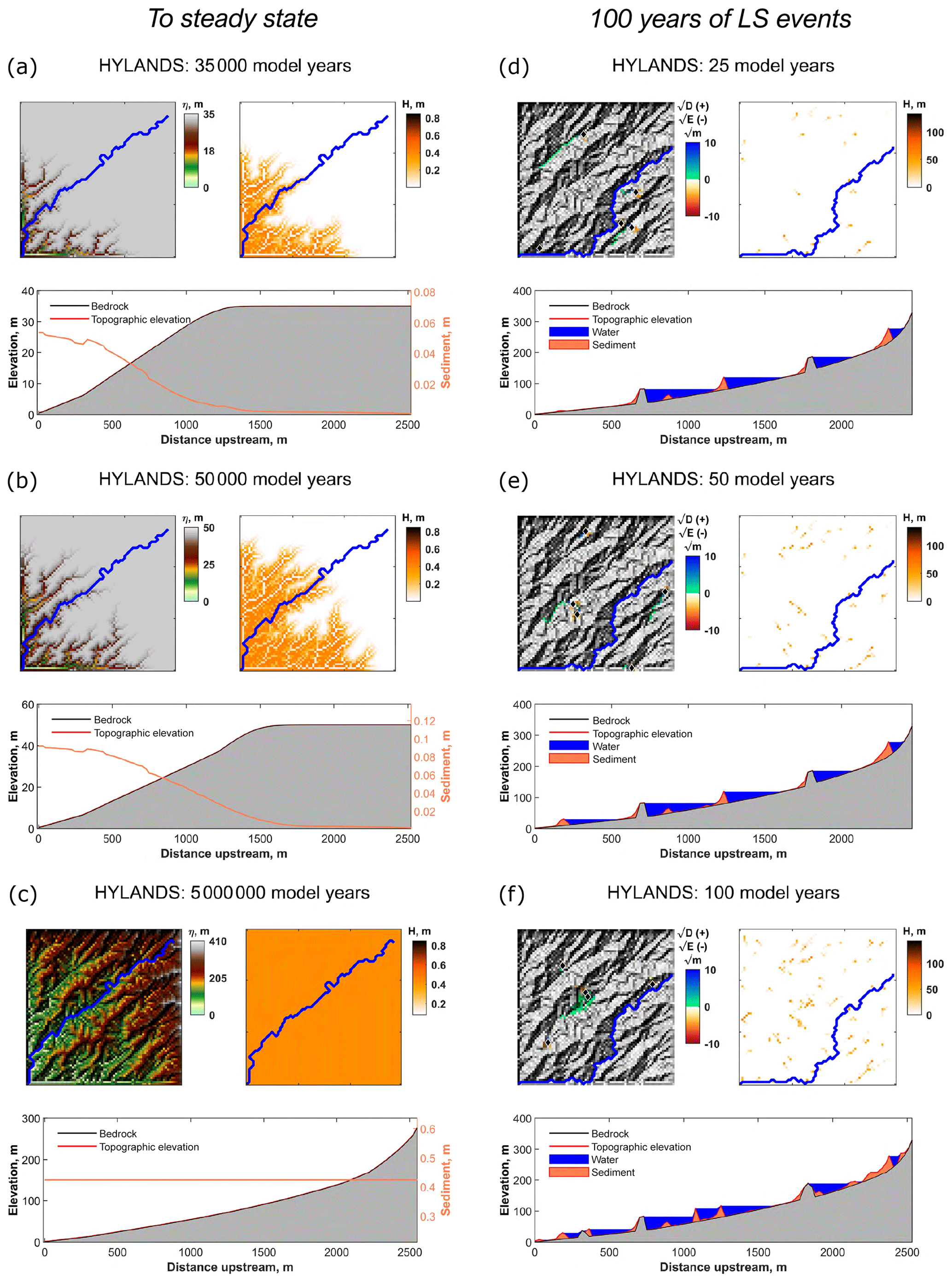
Figure 9 Synthetic model run showing landscape evolution to steady state followed by an intense landsliding period of 100 years. (a–c) Time slices showing evolution of the landscape to steady state, before the landslide period. The upper-left subplots show the evolution of topography through time. The upper-right subplots show the evolution of sediment thickness (H) through time. On both subplots, the blue line represents the location of the river plotted in the lower subplots. These lower subplots show the topographic and bedrock elevation (red and black line, respectively). The difference between the topographic elevation and the elevation of the bedrock represents the sediment thickness. With respect to total elevation, sediment thickness is small, so sediment thickness (orange line) is also plotted against the righthand y axis. The grey shaded area represents bedrock underlying the river profile. (d–f) Time slices showing the landslide period where intense landsliding is occurring over a period of 100 years. The upper-left subplots show the landslide activity. The location of landslides is indicated with black diamonds. The colors represent the square root of the landslide erosion (−) and deposition (+) during the presented time step. The upper-right subplots show the evolution of sediment thickness (H) through time. On both subplots, the blue line represents the location of the river plotted in the lower subplots. These lower subplots show the topographic and bedrock elevation (red and black line, respectively) as well as the volume occupied by sediments and water (orange and blue shaded area, respectively). Note that, during landsliding, both pure landslide dams arise as well as irregularities in the bedrock profile (the grey bumps). The latter originate from the river being redirected after landsliding, forming epigenetic gorges (see text).

The model run consists of three stages. In the first stage, the model is run to a steady state. For reasons of comparability, we simulate landscape evolution on a grid similar to the one used for the verification runs (Sect. 3), i.e., with a single open boundary cell in the southwestern corner. To simulate more realistic landscape scales, we use a domain of 75 by 75 cells with a higher resolution of 20 m. A complete overview of model parameter values is given in Table 1. The evolution of the landscape over time is shown in a series of time slices (Fig. 9a–c). Model behavior at this stage is as expected for the SPACE river erosion model when hillslope processes are not explicitly simulated (Shobe et al., 2017). During the first time steps, the drainage network establishes, and the landscape gradually approaches a steady state with uniform sediment thickness across the entire landscape.

In the second stage (Fig. 9d–f), we simulate a period of intense landslide activity by triggering a large number of landslides. Landslides are initiated based on their probability of sliding (Eq. 7) assuming an internal friction angle of 35^∘ and a low landslide return time $(t_{\mathrm{LS}}=\mathrm{2}\times {\mathrm{10}}^{\mathrm{3}}$ years). Under this configuration, many of the steep portions of the landscape become prone to landslide erosion and transform into a landslide source area. We assume that 25 % of the landslide-derived sediment is instantaneously evacuated out of the system as fine material ($F_{{\mathrm{f}}_{\text{hill}}}=\mathrm{0.25}$). Landslides trigger the formation of landslide dams, resulting in flooded river sections. Landslide dams not only alter the topographic elevation of the simulated domain but also change the drainage network. The location of the riverbed can change due to landslides and landslide-derived sediment rearranging the valley-bottom topography.

Immediately after the intense landsliding period, the trunk stream of the drainage network is still choked with sediment, and landslide dams are abundant (Fig. 10a–f). In the first few thousand years following the intense landsliding period, the lakes gradually fill with sediment. After 1500 years, most of the landslide-dammed lakes are filled with sediment. The fluvial profile is now characterized by a chain of knickpoints characteristic for fluvial profiles experiencing the delivery of debris by landslides (Ouimet et al., 2007) or other hillslope processes (Shobe et al., 2016, 2018). Where the in-channel bedrock is not covered with sediment, river incision into bedrock continues. However, upstream of landslide dams, the bed is choked with sediment, and the alluvial cover is too thick for bedrock incision to continue. As bedrock uplift continues and sediment is slowly evacuated from filled lakes, the bedrock profile adjusts, and small knickpoints are created along the river profile. While the specific cause is different (landslide dams ponding sediment vs. delivery of large-grained colluvium), the mechanism of knickpoint generation is similar to the numerical simulations of Shobe et al. (2016, 2018) in that a bare-bedrock reach downstream of a sediment-mantled reach can undergo faster erosion, thereby generating knickpoints that are decoupled from the base-level signal.

There are two distinct mechanisms for the generation of irregularities in the channel profiles: drainage rerouting due to landslide dams and knickpoint generation due to spatially varying sediment cover triggering differential erosion. The former mechanism can result in reaches where the bedrock slope is adverse relative to the water surface slope (the bumps in the bedrock profile in Figs. 9 and 10). The latter creates variability in the magnitude but not the direction of the bedrock slope. The drainage rerouting mechanism dominates in the simulations presented here and results in the formation of epigenetic river gorges (Fig. 10). Epigenetic gorges are characterized by rivers incising into the bedrock of former valley walls due to the blockage of the formal channel by landslide-derived sediment (Ouimet et al., 2008).

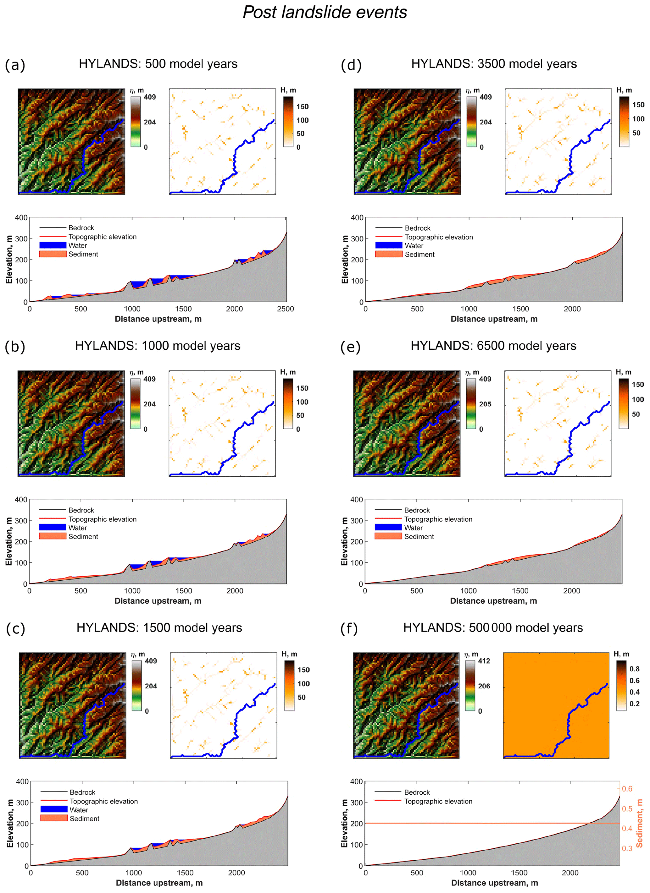
Figure 10 Synthetic model run showing recovery from intense landsliding illustrated in Fig. 9. (a–f) Time slices showing reestablishment of the landscape to steady state. Bedrock bumps created by landslide-induced drainage redirection are eroded, and the channel reattains its smoothly concave-up, steady-state configuration. For a detailed description of subplots and labels, see Fig. 9.

4 Discussion

Landscapes are the outcome of external perturbations, such as climate or tectonic variability, and internal dynamics originating from the coupling between fluvial incision and hillslope response (Burbank and Anderson, 2011; Glade et al., 2019). Much effort has been devoted to understanding the relationship between fluvial erosion efficiency and climate variability both through theoretical developments (Tucker, 2004; Lague, 2014) and observations (DiBiase and Whipple, 2011; Ferrier et al., 2013). A main finding is that the role of allogenic fluvial response (i.e., transient adjustment to an external perturbation) can only be understood when considering autogenic fluvial dynamics such as the existence of incision thresholds (Snyder et al., 2003; Lague et al., 2005) and the internal lithological heterogeneity in a landscape (Campforts et al., 2020; Glade et al., 2019). However, the role of landslides in long-term landscape evolution, especially the dynamic interaction between river incision and landslide activity, is only poorly understood. HyLands offers a tool to study dynamic feedbacks between landslides and river incision. The role of sediment dynamics in altering fluvial erosion and sediment transport is clearly illustrated in the numerical experiment (Figs. 9 and 10) where 5–10 kyr are required for the landscape to evolve back to a steady state after a pulse of landsliding. Not only does the delivery of landslide-derived sediment to the channel bed alter the topography of the channel profile but also it results in the formation of bedrock knickpoints and associated retreating incision waves. The HyLands output thereby corroborates earlier observations that landslides and tight channel–hillslope couplings in general are autogenic mechanisms altering the way in which landscapes respond to external (allogenic) perturbations (Ouimet et al., 2007; Shobe et al., 2016; Glade et al., 2019). HyLands is designed to study the dynamic feedbacks between landslides and river erosion at large spatial and temporal scales. To do so, the model integrates an algorithm for deep-seated landsliding with a recently proposed model for fluvial incision (Shobe et al., 2017). HyLands enables simulations over several millions of years and reproduces analytical predictions for fluvial dynamics and observed landslide scaling relationships.

4.1 Fluvial component

The SPACE river erosion model, which governs river evolution in HyLands, advances on existing river incision models in that it explicitly simulates the role of sediment in reducing the efficiency of bedrock incision (Beaumont et al., 1992; Lague, 2010). However, like SPACE, HyLands does not simulate the effect of increased bedrock incision efficiency due to mobile sediment acting as eroding tools (Sklar and Dietrich, 2004). Field observations warrant consideration of the tool effect (Cook et al., 2013; Beer et al., 2017), and theoretical predictions have shown that the interaction between sediment and bedrock incision is adjusted when the tool effect is considered (Gasparini et al., 2007). The impact of explicitly simulating the tool effect due to landslide-derived sediment has been evaluated in a numerical modeling study (Egholm et al., 2013). Egholm et al. (2013) concluded that landslide activity and its delivery of abrasive agents to the channel accelerate fluvial incision in actively uplifting mountain regions, whereas the lack of landslides in tectonically inactive mountain ranges strongly decreases erosion efficiency and enables topographic preservation. Adding the tool effect and evaluating its potential importance is therefore a primary goal for further model development in HyLands. Simulating the tool effect of sediments can be achieved by making the bedrock erosion function dependent (Eq. 4) on the sediment discharge Q_s (see e.g., Gasparini et al., 2007; Hobley et al., 2011; Zhang et al., 2018).

Like SPACE, HyLands does not include process-based approaches (Kean and Smith, 2004; Wobus et al., 2006; Davy and Lague, 2009; Coulthard et al., 2013), simplified adjustment rules (Lague, 2010; Yanites, 2018) or empirical closures (Attal et al., 2008) to dynamically calculate river width adjustments though time. HyLands assumes a relationship between drainage area and river width depending on the scaling exponent m (fixed in our simulations to 0.5; see also Table 1). It has however been shown that river width might vary as a function of sediment discharge or under varying tectonic configurations (Amos and Burbank, 2007; Turowski et al., 2009; Pfeiffer et al., 2017). Recent work using a two-dimensional hydro-sedimentary numerical model (Davy et al., 2017) based on the Saint-Venant equations has shown that river reorganization and narrowing after landslide events might strongly increase sediment transport capacity and alter sediment evacuation time after large landslide events (Croissant et al., 2017). While simulating dynamic river width reorganization at the landscape scale is currently not possible over longer timescales due to computational limitations, generic approximations for landslide-triggered channel narrowing (Croissant et al., 2019) could be integrated in future versions of HyLands.

4.2 Landslides

The landslide algorithm in HyLands is based on finite slope mechanics and assumes a planar rupture geometry. Although our approach reproduces observed magnitude–frequency and area–volume scaling relationships and is supported by previous work where landslides have been simulated using planar rupture surfaces (Jeandet et al., 2019), the use of more advanced rupture plane geometries has been proposed. Gallen et al. (2015) for example propose the use of concave-upward rupture planes to simulate coseismic landsliding. However, their approach is based on the statistical aggregation of one-dimensional slope-stability solutions and therefore simplifies the three-dimensional complexity of the topographic surface. Evaluating the role of varying rupture plane geometries in three dimensions is one of the potential future developments of HyLands.

At this stage HyLands does not explicitly simulate shallow landsliding, which typically occurs at the interface between the bedrock and the overlying sediment/regolith cover. Given the existing ability of HyLands to simultaneously simulate bedrock evolution and sediment thickness, adding a shallow landslide algorithm is feasible (Montgomery and Dietrich, 1994; Claessens et al., 2007) and would further our understanding of the coupling between climate variability and landscape stability (Parker et al., 2016). For shallow landslides to be added as a component in HyLands, the implementation and calibration of a regolith formation and soil flux model will be required (Campforts et al., 2016). Using additional model components to simulate soil formation and transport requires calibration of several additional processes components; care is needed to prevent over-calibration and over-parameterization of the model (Van Rompaey and Govers, 2002).

Our probabilistic sliding mechanism neglects seismic or hydrological landslide triggers (e.g., Keefer, 1984, 2002; Keefer and Larsen, 2007; Marc et al., 2015, 2018, 2019). Rather we simulate landslides as a stochastic process based on the mechanical stability of slope patches. Future developments could however adjust the spatial probability of landsliding by coupling an explicit earthquake model to HyLands (see Croissant et al., 2019). The probability of coseismic landslide activity can then be directly obtained by using constrained relationships between peak ground acceleration (PGA) and landslide initiation probabilities (Meunier et al., 2007).

HyLands uses a nonlinear, multiple-flow sediment redistribution scheme depending on topographic slope. Accurately simulating landslide sediment run-out distances is however a challenging process which is difficult to constrain and often simulated using empirical approximations (e.g., based on the absolute height difference within a landslide; Claessens et al., 2007). A potential way to validate and calibrate landslide runout distance would be to compare landslide-derived sediment distributions simulated with HyLands with runout distances simulated with higher-complexity models (Iverson, 2000; George, 2011; Zhou et al., 2020) or medium-complexity approaches such as RAMMS or Flow-R (Horton et al., 2013; Fan et al., 2017). Nevertheless, in its current form, HyLands reproduces characteristics of landscapes and channel profiles dominated by deep-seated landslides (Ouimet et al., 2007) and is, therefore, a useful tool to study the interaction between river incision and landslide dynamics at landscape evolution space scales and timescales.

4.3 Calibration of HyLands

A main challenge when applying HyLands in real settings is the calibration of both the river incision and landslide parameters. The power of any LEM lies in its capacity to integrate data over multiple spatial and temporal scales. Therefore, a range of datasets can be used to constrain model parameters. We identify three main categories of potential calibration data.

1. First are Topographic parameters that can be derived from DEMs. These include a range of metrics describing river characteristics (drainage density, river steepness, river stream power), hillslope properties (slope distribution, mean and median slope angles, aspect) and landslide scaling relationships (magnitude–frequency and area–volume distributions). All these metrics can be derived from topographic data and subsequently used to constrain HyLands erosion parameters (see Fig. 7).

2. Second are data directly constraining the integrated effects of river incision or landslide erosion. Ongoing efforts to map mass movements in landslide-prone areas now enable estimates of erosion rates over decadal timescales (Hovius et al., 1997; Larsen and Montgomery, 2012). Data on sediment redistribution following landslide events are however more difficult to collect (Fan et al., 2019). Although initial compilations now exist of global landslide sediment mobilization rates (Broeckx et al., 2020), such inventories remain incomplete. Data on landslide mobilization rates can be used to train HyLands while, in turn, HyLands can be used to further extend datasets on landslide mobilization rates and predict landslide sediment production rates in regions which are otherwise difficult to access.

3. Third are catchment-averaged cosmogenic radionuclide (CRN)-derived erosion rates. CRN data have been used to calibrate river incision models that explicitly integrate the stochastic nature of fluvial incision over time (DiBiase and Whipple, 2011; Scherler et al., 2017; Campforts et al., 2020). However, CRN data are sensitive to landslide activity (Niemi et al., 2005; Yanites et al., 2009; Wang et al., 2017; Tofelde et al., 2018), and the calibration of stochastic river incision models has been shown to be sensitive to landslide activity (Campforts et al., 2020). HyLands directly simulates stochastic landsliding and hence enables explicit simulation of the impact of landsliding on CRN-derived erosion rates.

4.4 Potential applications

Given the capacity of HyLands to explicitly simulate the interaction between fluvial dynamics and landslide triggering, it provides a unique toolbox to advance the field of geomorphology on several fronts. In the following we outline two example applications.

First, HyLands can be used as an experimental environment to test how landslides influence landscape response to external perturbations. Landslides are known to mediate long-term landscape evolution (Korup, 2005; Korup et al., 2007). By altering sediment discharge, landslides fundamentally alter the dynamic equilibrium between hillslopes and rivers, resulting in long-term implications for landscape evolution (Egholm et al., 2013). Moreover, large landslides are reported to critically alter drainage networks by causing major river captures (Korup et al., 2007; Dahlquist et al., 2018). A particular question which remains open for debate is the way in which landslides influence the evolution of a landscape to steady state. Although the stochastic nature of landslides prevents landscapes from evolving towards perfectly time- and space-invariant topographies, landslide-influenced landscapes will evolve towards a quasi-steady state if external drivers such as climate and tectonics remain constant. Though the study of steady-state landscapes improves our mechanistic understanding of landscape evolution, an even more interesting and challenging question would be to study the impact of landslides on the dynamic evolution of a landscape towards such a steady state. The latter problem is more relevant for most real-world landscapes, which are thought to be transient rather than in steady state (Mudd, 2017).

Second, HyLands can be used to evaluate the response of a landscape to a major landslide triggering event and to understand the timescales over which landslide-derived sediments are exported from the landscape (Wang et al., 2015; Li et al., 2016; Schwanghart et al., 2016; Robinson et al., 2017; Roback et al., 2018). As illustrated in this paper, a landscape requires a certain response time to recover from a landslide event – or a series of landslide events – and to evolve back to a steady-state configuration (Fig. 10). Landslide activity is typically manifested in downstream sediment dynamics, and LEMs are the right tool to simulate large-scale landscape response to landslide activity in upstream mountain regions. HyLands will enable prediction of downstream sediment response to landsliding, provided that the model can be calibrated effectively (Sect. 4.3).

5 Conclusions

We presented a new, fully coupled model for river incision into bedrock, sediment transport and bedrock landsliding. HyLands couples a mass conservative, sediment-discharge-dependent river incision model (SPACE; Shobe et al., 2017) with a deep-seated landslide algorithm (Densmore et al., 1998) and a multiple-flow sediment redistribution algorithm (Carretier et al., 2018). HyLands is designed to simulate landscape evolution at large temporal and spatial scales. The fluvial component of the model matches known, steady-state analytical solutions developed in earlier work (Davy and Lague, 2009; Shobe et al., 2017). Landslides produced by HyLands replicate observed scaling relationships, indicating the realism of the simulations. HyLands is implemented in the TopoToolbox GIS interface (Schwanghart and Scherler, 2014), thereby facilitating the use of rasterized field data for calibration and providing direct access to a wide range of GIS analysis tools. In an example application, we illustrated how HyLands can be used to evaluate the impact of landslide activity on fluvial and hillslope characteristics. We showed how landslide activity triggers the formation of landslide-dammed lakes and how HyLands is capable of simulating subsequent lake infilling and knickpoint formation, similar to reported landscape changes following landslide activity (Ouimet et al., 2007). The foremost advantage of HyLands is its capacity to explicitly simulate the role of landslides, landslide-derived sediment and fluvial dynamics at the landscape scale. The model is well suited to address a range of new questions related to how channel–hillslope coupling modulates landscape evolution and response to perturbations.