Development of the global atmospheric chemistry general circulation model BCC-GEOS-Chem v1.0: model description and evaluation

Chemistry plays an indispensable role in investigations of the atmosphere; however, many climate models either ignore or greatly simplify atmospheric chemistry, limiting both their accuracy and their scope. We present the development and evaluation of the online global atmospheric chemical model BCC-GEOS-Chem v1.0, coupling the GEOS-Chem chemical transport model (CTM) as an atmospheric chemistry component in the Beijing Climate Center atmospheric general circulation model (BCC-AGCM). The GEOS-Chem atmospheric chemistry component includes detailed tropospheric HO_x–NO_x–volatile organic compounds–ozone–bromine–aerosol chemistry and online dry and wet deposition schemes. We then demonstrate the new capabilities of BCC-GEOS-Chem v1.0 relative to the base BCC-AGCM model through a 3-year (2012–2014) simulation with anthropogenic emissions from the Community Emissions Data System (CEDS) used in the Coupled Model Intercomparison Project Phase 6 (CMIP6). The model captures well the spatial distributions and seasonal variations in tropospheric ozone, with seasonal mean biases of 0.4–2.2 ppbv at 700–400 hPa compared to satellite observations and within 10 ppbv at the surface to 500 hPa compared to global ozonesonde observations. The model has larger high-ozone biases over the tropics which we attribute to an overestimate of ozone chemical production. It underestimates ozone in the upper troposphere which is likely due either to the use of a simplified stratospheric ozone scheme or to biases in estimated stratosphere–troposphere exchange dynamics. The model diagnoses the global tropospheric ozone burden, OH concentration, and methane chemical lifetime to be 336 Tg, 1.16×10⁶ molecule cm⁻³, and 8.3 years, respectively, which is consistent with recent multimodel assessments. The spatiotemporal distributions of NO₂, CO, SO₂, CH₂O, and aerosol optical depth are generally in agreement with satellite observations. The development of BCC-GEOS-Chem v1.0 represents an important step for the development of fully coupled earth system models (ESMs) in China.

1 Introduction

Atmospheric chemistry plays an indispensable role in the evolution of atmospheric gases and aerosols and is also an essential component of the climate system due to its active interactions with atmospheric physics and biogeochemistry on various spatiotemporal scales. Climate modulates the natural emissions, chemical kinetics, and transport of atmospheric gases and aerosols, while changes in many of these constituents alter the radiative budgets of the climate system and also influence the biosphere (Jacob and Winner, 2009; Fiore et al., 2012; Lu et al., 2019a). Climate–chemistry coupled models are indispensable tools to quantify climate–chemistry interactions and to predict future air quality. However, coupling transport and chemistry of hundreds of chemical species on all spatiotemporal scales in climate system models (CSMs) poses a considerable challenge for model complexity and computational resources. Only 10 of the 39 CSMs in phase 5 of the Coupled Model Intercomparison Project (CMIP5) simulated atmospheric chemistry interactively (IPCC AR5, 2013). In the other models, including all the five Chinese CSMs, chemically active species were prescribed. The development of a climate–chemistry coupled model has been identified as a research frontier for atmospheric chemistry (National Research Council, 2012), and also a priority for CSM development particularly in China. An initiative to include the online simulation of atmospheric chemistry in CSMs, as an essential step toward building a climate–chemistry coupled model, was launched by the Beijing Climate Center (BCC) at the China Meteorological Administration (CMA) after CMIP5.

Here we present the development of the global atmospheric chemistry general circulation model BCC-GEOS-Chem v1.0, which enables online simulations of atmospheric chemistry in the BCC-CSM version 2 (BCC-CSM2). BCC-GEOS-Chem is built on the coupling of the GEOS-Chem chemical module with the BCC atmospheric general circulation model (BCC-AGCM), the atmospheric component of the BCC-CSM2. BCC-CSM2 is a fully coupled global CSM in which the atmosphere, land, ocean, and sea-ice components interact with each other through the exchange of momentum, energy, water, and carbon (Wu et al., 2008, 2013, 2019). The earlier version of BCC-CSM (v1.1 and v1.1m) was enrolled in CMIP5 and has been widely applied to weather and climate research (e.g., Wu et al., 2013, 2014; Xin et al., 2013; Zhao and He, 2015). It has been recently updated to BCC-CSM2 and is being used in that configuration for the Coupled Model Intercomparison Project Phase 6 (CMIP6) (Wu et al., 2019). GEOS-Chem (http://geos-chem.org, last access: 10 July 2020), originally described by Bey et al. (2001), is a global three-dimensional chemical transport model (CTM) which includes detailed state-of-the-art gas–aerosol chemistry and which is used by a large international community for a broad range of research on atmospheric chemistry, is continually updated with scientific innovations from users, is rigorously benchmarked, and is openly accessible on the cloud (Zhuang et al., 2019). The model is continually evaluated with atmospheric observations from its user community (e.g., Hu et al., 2017). The integration of BCC-AGCM and GEOS-Chem for online simulations of global atmospheric chemistry will have attractive scientific and operational applications (e.g., sub-seasonal air quality prediction), and it also represents an important step for the development of fully coupled earth system models (ESMs) in China.

Until recently, the offline GEOS-Chem CTM relied exclusively on fixed latitude–longitude grids and was designed for shared-memory (OpenMP) parallelization. With such features, the GEOS-Chem CTM was not flexible enough to be coupled with BCC-CSM, which typically runs on spectral space (with adjustable options for the grid type and resolution dependent on the wave truncation number) and requires vast computational resources. The integration of GEOS-Chem chemical module into CSMs has been enabled by separating the module (which simulates all local processes including chemistry, deposition, and emissions) from the simulation of transport and making it operate on one-dimensional (vertical) columns in a grid-independent manner (Long et al., 2015; Eastham et al., 2018). The GEOS-Chem chemical module can thus be coupled with a CSM on any grid, and the CSM simulation of dynamics then handles chemical transport. GEOS-Chem used as an online chemical module in CSMs shares the exact same code as the classic offline GEOS-Chem for local processes (chemistry, deposition, and emissions) (Long et al., 2015). This capability ensures that the scientific improvements of GEOS-Chem contributed by the worldwide research community can be conveniently incorporated into CSMs, allowing the chemistry of BCC-GEOS-Chem to be trackable to the latest GEOS-Chem version. Previous studies have demonstrated the success of coupling GEOS-Chem into the NASA GEOS-5 Earth system model and more recently the Weather Research and Forecasting (WRF) mesoscale meteorological model as an online atmospheric chemistry module (Long et al., 2015; Hu et al., 2018; Lin et al., 2020).

This paper presents the overview of the BCC-GEOS-Chem v1.0 model and evaluates the model simulation of present-day atmospheric chemistry. The model framework and its components are described in Sect. 2. We conducted a 3-year (2012–2014) model simulation to demonstrate the model's capability and for model evaluation. In Sect. 3, we compare simulated gases and aerosols with satellite and in situ observations and also diagnose the global tropospheric ozone burden and budget. Future plans for model development and summary are presented in Sect. 4.

2 Development and description of the BCC-GEOS-Chem v1.0

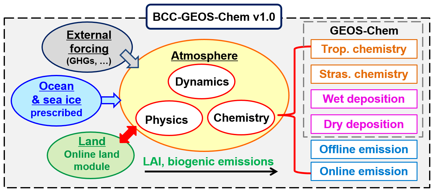
Figure 1 presents the framework of the BCC-GEOS-Chem v1.0. BCC-GEOS-Chem v1.0 includes interactive atmosphere (including dynamics, physics, and chemistry) and land modules, and other components such as ocean and sea ice are configured as boundary conditions for this version. The atmospheric dynamics and physics module (Sect. 2.1) and the land module (Sect. 2.2) come from the BCC-AGCM version 3 and the BCC Atmosphere and Vegetation Interaction Model version 2 (BCC-AVIM2), respectively. Atmosphere and land modules exchange the fluxes of momentum, energy, water, and carbon through the National Center for Atmospheric Research (NCAR) flux coupler version 5. Dynamic and physical parameters from both the atmosphere (e.g., radiation, temperature, and wind) and the land (e.g., surface stress and leaf area index) modules are then used to drive the GEOS-Chem chemistry (Sect. 2.3) and deposition (Sect. 2.4) of atmospheric gases and aerosols. Anthropogenic and biomass burning emissions are from the inventories used for the CMIP6 (Sect. 2.5.1). A number of climate-sensitive natural emissions such as biogenic and lightning emissions are calculated online in the model (Sect. 2.5.2). Boundary conditions, external forcing, and experiment design are described in Sect. 2.6.

Figure 1 Schematic diagram of the BCC-GEOS-Chem v1.0 model framework.

2.1 The atmospheric model BCC-AGCM3

BCC-AGCM3 is a global atmospheric spectral model. It has adjustable horizontal resolution and 26 vertical hybrid layers extending from the surface to 2.914 hPa. In this study we use the default horizontal spectral resolution of T42 (approximately 2.8^∘ latitude × 2.8^∘ longitude). The dynamical core and physical processes of the BCC-AGCM3 have been described comprehensively in Wu et al. (2008, 2010) with recent updates documented in Wu et al. (2012, 2019). Wu et al. (2019) showed that the BCC-CSM2 (BCC-AGCM3 as the atmospheric model) captured well the global patterns of temperature, precipitation, and atmospheric energy budget. BCC-CSM2 also showed significant improvements in reproducing the historical changes in global mean surface temperature from the 1850s and climate variabilities such the Quasi-Biennial Oscillation (QBO) and the El Niño–Southern Oscillation (ENSO) compared with its previous version BCC-CSM1.1m (Wu et al., 2019). Here we present a brief summary of the main features in BCC-AGCM3.

The governing equations and physical processes (e.g., clouds, precipitation, radiative transfer, and turbulent mixing) of BCC-AGCM3 originated from the Eulerian dynamic framework of the Community Atmosphere Model (CAM3) (Collins et al., 2006), but substantial modifications have been incorporated. Wu et al. (2008) introduced a stratified reference of atmospheric temperature and surface pressure to the governing equations. In this way, prognostic temperature and surface pressure in the original governing equation can be derived from their prescribed reference plus the prognostic perturbations relative to the reference. Resolving algorithms (e.g., explicit and semi-implicit time difference schemes) were adapted accordingly. The modified dynamic framework reduced the truncation errors in the model, as well as the bias due to inhomogeneous vertical stratification, and therefore improved the descriptions of the pressure gradient force and the vertical temperature structure (Wu et al., 2008). BCC-AGCM3 also implements a new mass-flux cumulus scheme to parameterize deep convection (Wu, 2012). The revised deep convection parameterization by including the entrainment of environment air into the uplifting parcel better captured the realistic timing of intense precipitation (Wu, 2012) and the Madden–Julian Oscillation (MJO) (Wu et al., 2019). Other important updates of atmospheric physical processes in BCC-AGCM3 relative to CAM3 include a new dry adiabatic adjustment to conserve the potential temperature, a modified turbulent flux parameterization to involve the effect from waves and sea spray on ocean surface latent and sensible heat, a new scheme to diagnose cloud fraction, a revised cloud microphysics scheme to include the indirect effects of aerosol based on bulk aerosol mass, and modifications for radiative transfer and boundary layer parameterizations (Wu et al., 2010, 2014, 2019).

2.2 The land model BCC-AVIM2

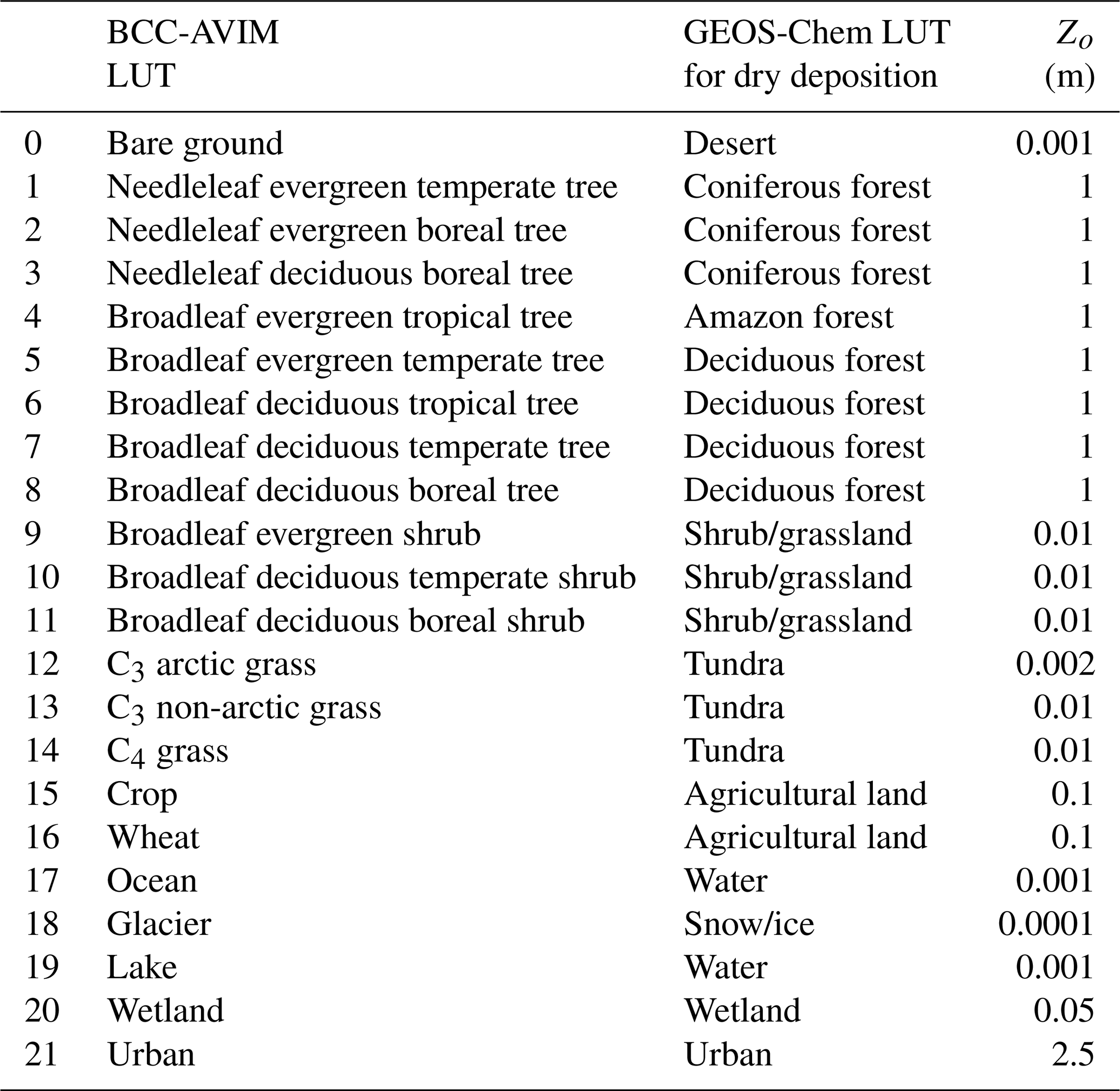
BCC-AVIM2 is a comprehensive land surface model originating from the Atmospheric and Vegetation Interaction Model (AVIM) (Ji, 1995; Ji et al., 2008) which serves as the land component in BCC-CSM2. It includes three submodules: the biogeophysical module, plant ecophysiological module, and soil carbon–nitrogen dynamic module. The biogeophysical module simulates the transfer of energy, water, and carbon between the atmosphere, plant canopy, and soil. It has 10 soil layers and up to 5 snow layers. The ecophysiological module describes the ecophysiological activities, such as photosynthesis, respiration, turnover, and mortality of vegetation, and diagnoses the induced changes in biomass. The soil carbon–nitrogen dynamic module describes the biogeochemical process such as the conversion and decomposition of soil organic carbon. The vegetation surface in BCC-AVIM2 is divided into 15 plant functional types (PFTs), as shown in Table 1, and each grid cell contains up to four PFTs. Wu et al. (2013) showed that the model captured well the spatial distributions, long-term trends, and interannual variability of global carbon sources and sinks compared to observations and other models. Recent improvements in BCC-AVIM2, such as the introduction of a variable temperature threshold for the thawing/freezing of soil water and improved presentations of snow surface albedo and snow cover fraction, are described in Li et al. (2019). Biogenic emissions and dust mobilizations are also implemented in BCC-AVIM2 interactively with the atmosphere, as will be described later in Sect. 2.5.

Table 1 Mapping of land use types (LUTs) used in BCC-GEOS-Chem v1.0 to the Wesely deposition surfaces for deposition. Also shown are the roughness heights (Z_o) for each LUT.

2.3 Atmospheric chemistry

We implement in this study the GEOS-Chem v11-02b “Tropchem” mechanism as the atmospheric chemistry module of BCC-GEOS-Chem v1.0. As described in the introduction, GEOS-Chem used as an online chemical module in ESMs shares the exact same codes for local terms (chemistry, deposition, and emissions) as the classic offline GEOS-Chem. Here, we use the GEOS-Chem chemical module to process the chemistry and deposition in BCC-GEOS-Chem v1.0 and operate emissions separately in the model, as will be described in Sect. 2.5.

GEOS-Chem v11-02b Tropchem mechanism describes advanced and detailed HO_x–NO_x–volatile organic compounds (VOCs)–ozone–bromine–aerosol chemistry relevant to the troposphere (Mao et al., 2010, 2013; Parrella et al., 2012; Fischer et al., 2014; Marais et al., 2016). It includes 74 advected species (tracers) and 91 non-advected species (http://wiki.seas.harvard.edu/geos-chem/index.php/Species_in_GEOS-Chem, last access: 10 July 2020). Tracer advection in BCC-GEOS-Chem v1.0 is performed using a semi-Lagrangian scheme (Williamson and Rasch, 1989), and the vertical diffusion within the boundary layer follows the parameterization of Holtslag and Boville (1993). Photolysis rates are calculated by the Fast-JX scheme (Bian and Prather, 2002). The simulation of sulfate–nitrate–ammonia (SNA) aerosol chemistry, four-size bins of mineral dust (radii of 0.1–1.0, 1.0–1.8, 1.8–3.0, and 3.0–6.0 µm), and two types of sea salt aerosols (accumulating mode: 0.01–0.5 µm; coarse mode: 0.5–8.0 µm) follows Park et al. (2004), Fairlie et al. (2007), and Jaeglé et al. (2011). Aerosol and gas-phase chemistry interact through heterogeneous chemistry on aerosol surface (Jacob, 2000; Evans and Jacob, 2005; Mao et al., 2013), aerosol effects on photolysis (Martin et al., 2003), and gas–aerosol partitioning of NH₃ and HNO₃ calculated by the ISORROPIA II thermodynamic module (Fountoukis and Nenes, 2007; Pye et al., 2009). Methane concentrations in the chemistry module are prescribed as uniform mixing ratios over four latitudinal bands (90^∘–30^∘ S, 30^∘ S–0^∘, 0^∘–30^∘ N, and 30^∘–90^∘ N), with the year-specific annual mean concentrations given by surface measurements from the NOAA Global Monitoring Division. Stratospheric ozone is calculated by the linearized ozone parameterization (LINOZ) (McLinden et al., 2000) and is transported to the troposphere driven by the model wind fields.

2.4 Dry and wet deposition

Dry and wet deposition for both gas and aerosols are parameterized following GEOS-Chem algorithms. Dry deposition is calculated online based on the resistance-in-series scheme (Wesely, 1989). The scheme describes gaseous dry deposition by three separate processes, i.e., the turbulent transport in the aerodynamic layer, molecular diffusion through the quasi-laminar boundary layer, and uptake at the surface. Aerosol dry deposition further considers the gravitational settling of particles as described in Zhang et al. (2001). Variables needed for the dry deposition calculation, such as the friction velocity, Monin–Obukhov length, and leaf area index (LAI), are obtained from atmospheric dynamics/physics modules or the land module BCC-AVIM, based on which GEOS-Chem calculates the aerodynamic, boundary layer, and surface resistances. The impacts of some other short-term land variables, such as stomatal conductance, on dry deposition are not included yet. We have also reconciled the land use types (LUTs) used in dry deposition with those used in BCC-AVIM following Geddes et al. (2016) and Zhao et al. (2017). The LUTs from BCC-AVIM are mapped directly onto the 11 deposition surface types used in GEOS-Chem, as shown in Table 1. Dry deposition velocity is calculated as the weighted average over all LUTs in each grid box.

Wet deposition of aerosols and soluble gases by precipitation in BCC-GEOS-Chem v1.0 includes the scavenging in convective updrafts, in-cloud rainout, and below-cloud washout (Liu et al., 2001). Following the implementation of GEOS-Chem chemical module to GEOS-5 ESM (Hu et al., 2018), the convective transport of chemical tracers and scavenging in the updrafts in BCC-GEOS-Chem v1.0 is performed using the GEOS-Chem convection scheme but with convection variables diagnosed from BCC-AGCM. This takes advantage of the existing capability of the GEOS-Chem scheme to describe gas and aerosol scavenging (Liu et al., 2001; Amos et al., 2012).

2.5 Emissions

2.5.1 Offline emissions

Historical anthropogenic emissions used in this study are mostly obtained from the Community Emissions Data System (CEDS) emission inventory (Hosely et al., 2017). CEDS is an updated global emission inventory which provides sectoral, gridded, and monthly emissions of reactive gases and aerosols from 1750 to 2014 for use in the CMIP6 experiment (Eyring et al., 2016; Hosely et al., 2018). Here we use the CEDS anthropogenic emissions of NO_x, CO, SO₂, NH₃, non-methane volatile organic compounds (NMVOCs), and carbonaceous aerosols (black carbon, BC, and organic carbon, OC) (Table 2). We also include three-dimensional aircraft emissions of several gases and aerosols in the model. The historical global biomass burning emission inventory is obtained from van Marle et al. (2017) which is also used for the CMIP6 experiment. We also incorporate emissions from the Atmospheric Chemistry and Climate Model Intercomparison Project (ACCMIP) inventory (http://accent.aero.jussieu.fr/ACCMIP.php, last access: 14 June 2020; Lamarque et al., 2010) and from Wu et al. (2020) for emissions not included in the CEDS dataset. These mainly apply to oceanic emissions, soil NO_x emissions, and volcanic SO₂ emissions. Several sources (e.g., oceanic acetaldehyde emissions; Millet et al., 2010; Wang et al., 2019) have not yet been included in this model version.

Table 2 Global annual emissions used in the BCC-GEOS-Chem v1.0 categorized by sectors (in Tg yr⁻¹).

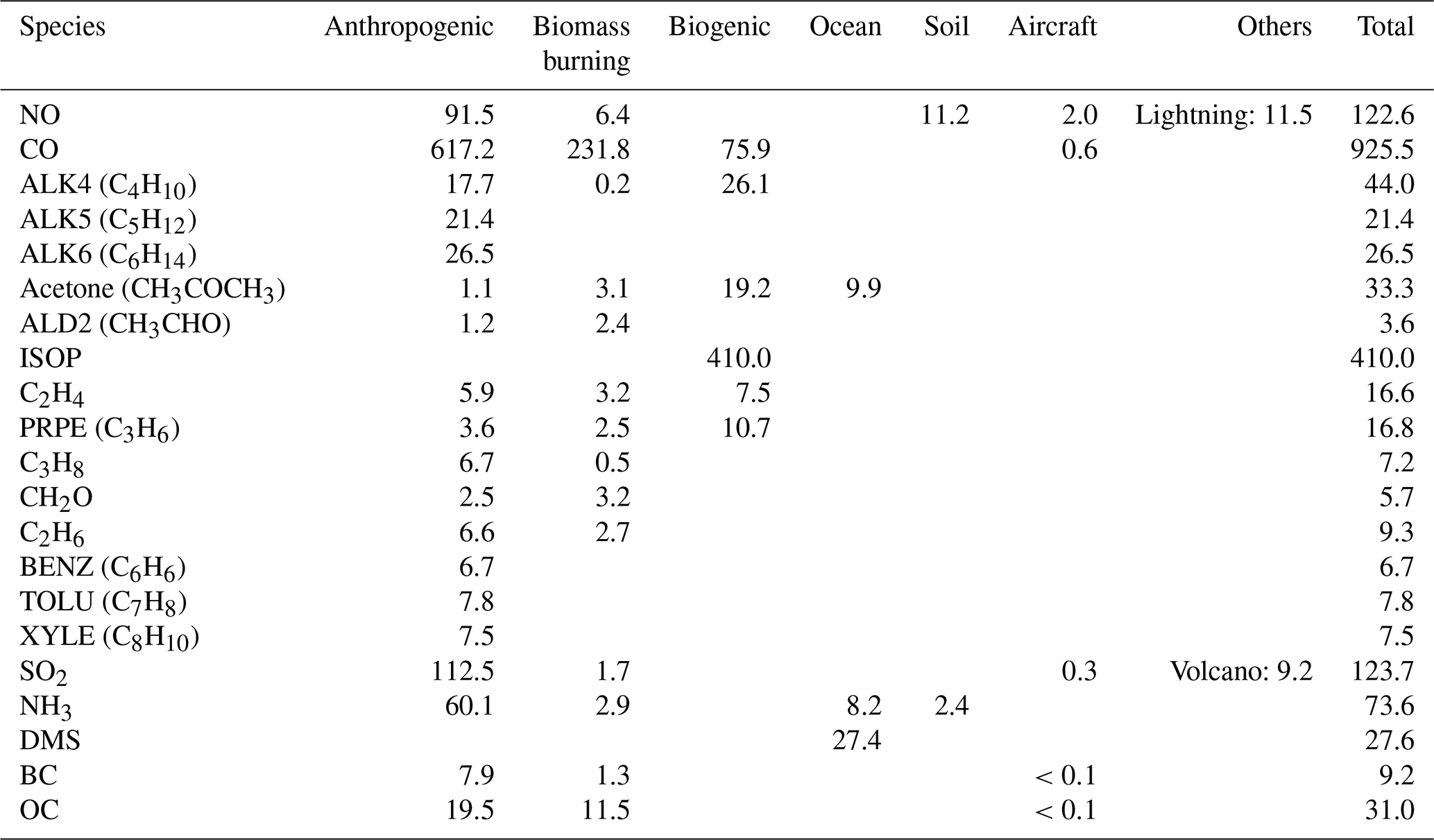
Table 2 lists the amount of annual total emissions of chemicals used in this study separated by emission sectors averaged over 2012–2014. Figure 2a and b show the spatial distributions of annual NO (not including lightning emissions which will be discussed below separately) and CO emissions. Global annual total emissions of NO (not including lightning emissions) and CO are 111.1 and 925.5 Tg yr⁻¹, respectively. The global anthropogenic emissions are relatively flat in 2012–2014 (e.g., from 614.7 to 619.6 Tg yr⁻¹ for CO), while the biomass burning emissions have much stronger interannual variability (e.g., varying from 209 to 256 Tg yr⁻¹ for CO). As pointed out by Hosely et al. (2018), CEDS anthropogenic emissions are generally higher than previous inventories. For instance, the anthropogenic NO_x and CO emissions are, respectively, about 10 % and 8 % higher compared to CMIP5 emissions in the 1980–2000 period. This is likely due to the updates of emission factors and inclusion of new emission sectors (Hosely et al., 2018). Compared to CMIP5, biomass burning emissions used in CMIP6 for year 2000 conditions are about 20 % and 30 % lower for CO and OC, respectively, but are about 17 % higher for NO_x (Fig. 13 in van Marle et al., 2017).

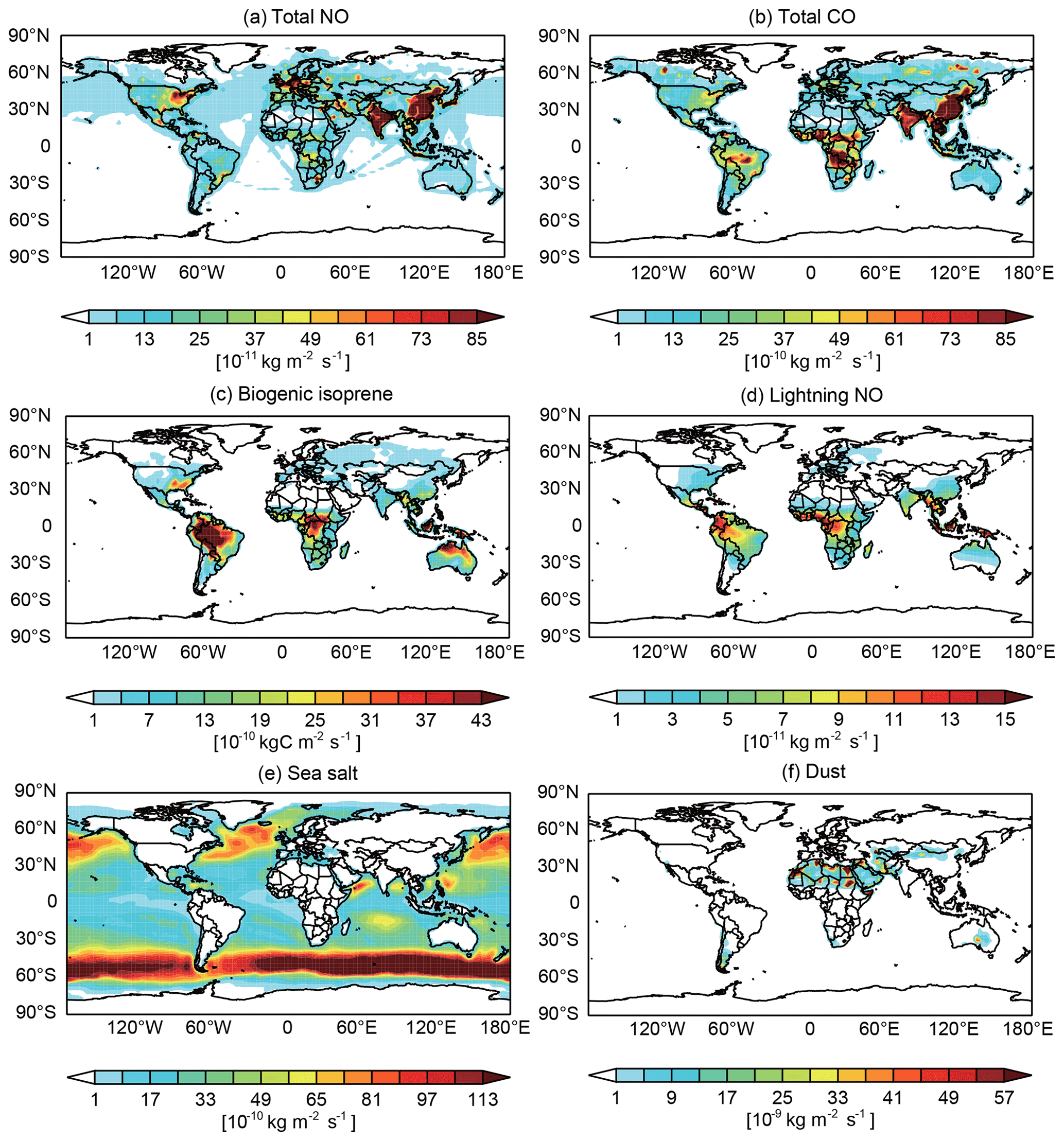
Figure 2 Spatial distributions of annual total emissions used in the study: (a) total NO emissions (not including lightning emissions), (b) total CO emissions, (c) biogenic isoprene emissions, (d) lightning NO emissions, (e) sea salt emissions (dry mass), and (f) mineral dust emissions.

2.5.2 Online emissions

BCC-GEOS-Chem v1.0 includes a number of climate-sensitive natural sources. Biogenic emissions of NMVOCs are calculated online using the Model of Gases and Aerosols (MEGAN) algorithm (Guenther et al., 2012) in the land module. MEGAN estimates biogenic emissions as a function of an emission factor at standard condition, a normalized emission activity factor relative to the standard condition, and a scaling ratio which accounts for canopy production and loss. The emission activity factor is further determined by surface or plant parameters such as leaf age and LAI diagnosed in BCC-AVIM, as well as meteorological variables such as radiation and temperature. The annual biogenic isoprene emissions calculated in BCC-GEOS-Chem v1.0 are 410.0 Tg yr⁻¹ averaged for the 2012–2014 period with a relatively small interannual variability (404.6 to 415.2 Tg yr⁻¹). This is close to but lower than estimates from the literature (500–750 Tg yr⁻¹; Guenther et al., 2012). The model captures the hot spots of biogenic isoprene emissions in the tropical continents and the southeastern United States (Fig. 2c).

The parameterization of lightning NO emissions follows Price and Rind (1992). The model diagnoses the lightning flash frequency in deep convection as a function of the maximum cloud top height (CTH). Lightning NO production is then calculated as a function of lightning flash frequency, fraction of intracloud (IC) and cloud-to-ground (CG) lightning based on the cloud thickness, and the energy per flash (Price et al., 1997). Vertical distributions of lightning NO emissions in the column follow Ott et al. (2010). The model estimates global annual total lightning NO emissions of 10.9 to 12.2 Tg NO yr⁻¹ for 2012–2014, in agreement with the best estimate of present-day emissions (10.7±6.4 Tg NO yr⁻¹ as summarized in Schumann and Huntrieser, 2007). The emissions are centered near the tropics due to strong convection, as shown in Fig. 2d.

The model also includes wind-driven sea salt and mineral dust emissions. Emission fluxes of sea salt aerosols are dependent on the sea salt particle radius and proportional to the 10 m wind speed with a power of 3.41 following the empirical parameterization from Monahan et al. (1986) and Gong et al. (1997). Mineral dust emissions are determined by wind friction speed, soil moisture, and vegetation type following the Dust Entrainment and Deposition (DEAD) scheme as described by Zender et al. (2003). Figure 2e and f show the spatial distributions of sea salt and mineral dust emissions, with their annual total emissions of 3963 and 1347 Tg, respectively, being consistent with previous estimates from Jaeglé et al. (2011) and Fairlie et al. (2007).

2.6 Boundary conditions, external forcing, and experiment design

BCC-GEOS-Chem v1.0 is configured using prescribed ocean and sea ice as boundary conditions. Historical sea surface temperature and sea-ice extents are obtained from the Earth System Grid Federation (ESGF) (https://esgf-node.llnl.gov/search/input4mips/ last access: 2 June 2019). These prescribed datasets are also used in CMIP6 atmosphere-only simulations. External forcing data, including historical greenhouse gas concentrations (CO₂, CH₄, N₂O, CFCs) (Meinshausen et al., 2017), land use forcing, and solar forcing, are also accessed from the ESGF (https://esgf-node.llnl.gov/search/input4mips/, last access: 10 July 2020). BCC-CSM2 has implemented the radiative transfer effects of greenhouse gases and aerosols, as well as the aerosol–cloud interactions, based on bulk aerosol mass concentrations (Wu et al., 2019). Since BCC-CSM2 does not include interactive atmospheric chemistry, the calculation of radiative transfer and aerosol–cloud interactions is based on historical gridded ozone concentrations from CMIP5- and CMIP6-recommended anthropogenic aerosol optical properties (Stevens et al., 2017). Here for BCC-GEOS-Chem v1.0, we follow BCC-CSM2 and use these prescribed ozone and aerosols rather than model online calculated values for feedback calculation. This is meant to focus on the modeling and evaluation of atmospheric chemistry in this work as the first step of the coupling. Interactive coupling of chemistry and climate through radiation and aerosol–cloud interactions will be considered in the next version of BCC-GEOS-Chem.

We conduct BCC-GEOS-Chem v1.0 simulations from 2011 to 2014. The initial conditions for atmospheric dynamics and physics in 2011 are obtained from the historical simulations (1850–2014) of BCC-CSM2 (Wu et al., 2019), and initial states of chemical tracers are obtained from the GEOS-Chem Unit Tester (http://wiki.seas.harvard.edu/geos-chem/index.php/Unit_Tester_for_GEOS-Chem_12, last access: 2 June 2019). Model results for 2012–2014 are evaluated.

3 Model evaluation

3.1 Observations used for model evaluation

We use an ensemble of surface, ozonesonde, and satellite observations to evaluate the BCC-GEOS-Chem v1.0 simulation of present-day atmospheric chemistry (Table 3). Ozonesonde measurements are obtained from the World Ozone and Ultraviolet Radiation Data Centre (WOUDC; http://woudc.org/data.php, last access: 2 June 2019) operated by the Meteorological Service of Canada. The network also includes sites from the Southern Hemisphere Additional Ozonesondes (SHADOZ; Thompson et al., 2003). To derive the monthly mean ozone profiles, only sites and months with more than three observations per month are considered, and simulated monthly mean ozone profiles are sampled over the corresponding model grids (Lu et al., 2019b). We further categorize the WOUDC observations into 10 regions following Tilmes et al. (2012) and Hu et al. (2017) for model evaluation, as shown in Fig. 3. We also use the Tropospheric Ozone Assessment Report (TOAR) surface ozone database (Schultz et al., 2017a) that provides ozone metrics (e.g., monthly mean) for more than 9000 monitoring sites around the world from the 1970s to 2014 (Schultz et al., 2017b). Surface aerosol measurements (sulfate, nitrate, OC, BC) over the United States are obtained from the Interagency Monitoring of Protected Visual Environments (IMPROVE) network. These aerosol measurements are 24 h averages every 3 d.

Table 3 Observational datasets used for model evaluation.

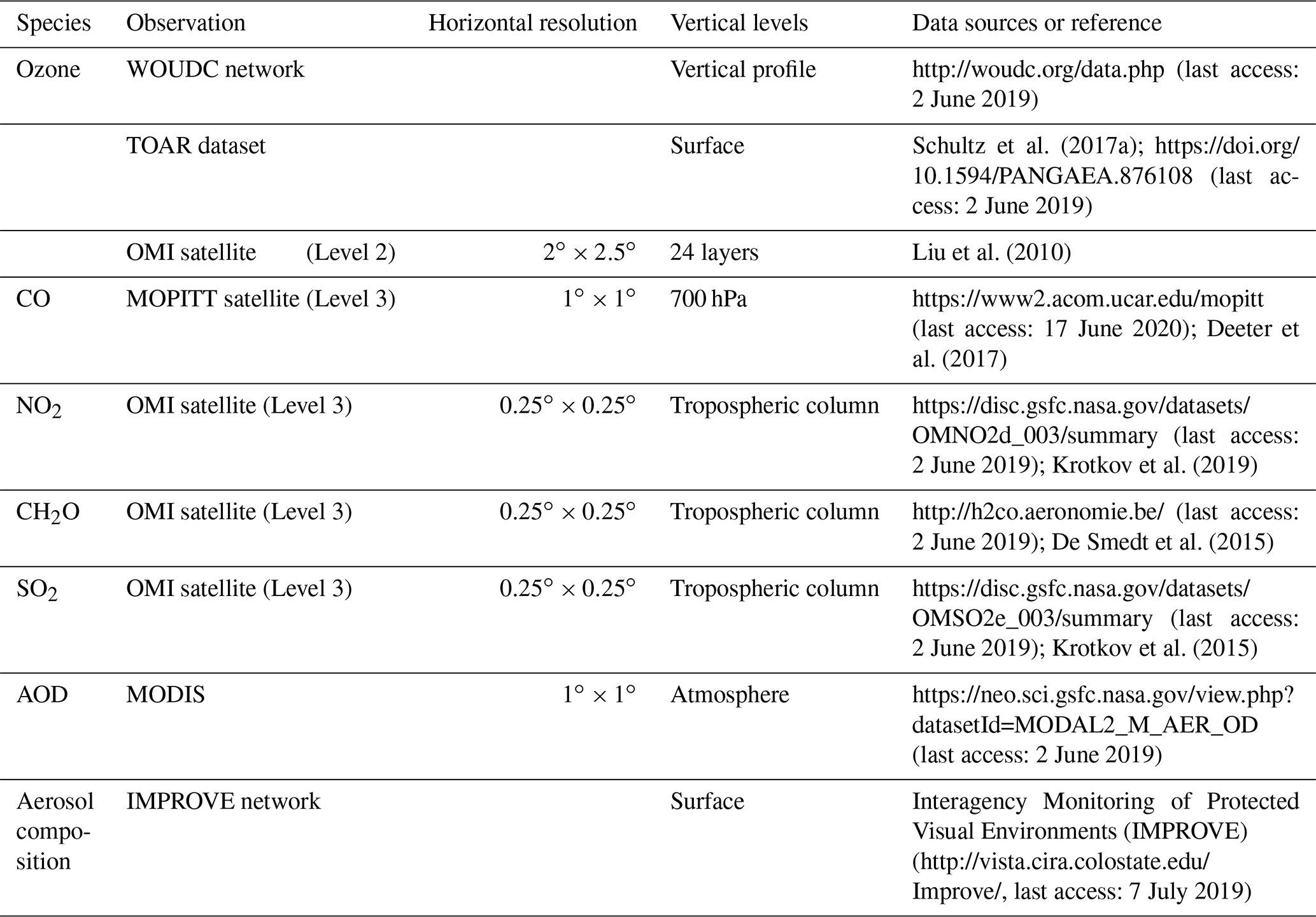
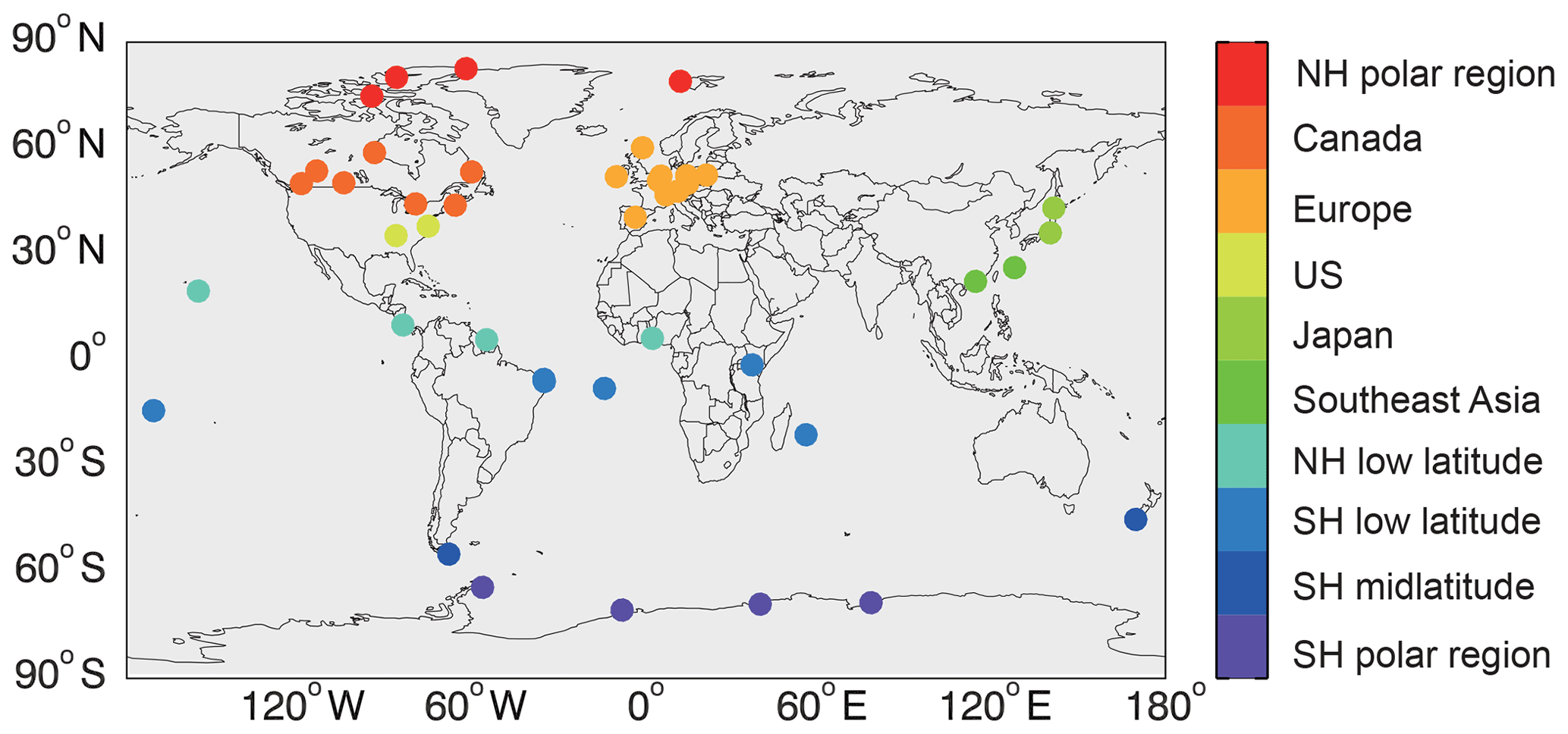
Figure 3 Locations of selected ozonesonde observations in 2012–2014 used in this study categorized by 10 regions.

Satellite products from the NASA Earth Observing System (EOS) Aura's Ozone Monitoring Instrument (OMI) are also used. We use the OMI ozone profile (PROFOZ) with 24 layers extending from the surface to 60 km retrieved by Liu et al. (2005, 2010) based on the optimal estimation technique (Rodgers, 2000). The OMI PROFOZ dataset has been comprehensively validated through comparisons with ozonesondes (Zhang et al., 2010; Hu et al., 2017; Huang et al., 2017) and satellite products (Huang et al., 2018). We also use the OMI gridded monthly mean tropospheric nitrogen dioxide (NO₂) column (Krotkov et al., 2013), formaldehyde (CH₂O) column (De Smedt et al., 2015), and planetary boundary layer (PBL) sulfur dioxide (SO₂) column (Krotkov et al., 2015). Other satellite observations include carbon monoxide (CO) observations from the Measurement of Pollution in the Troposphere (MOPITT) instrument (Deeter et al., 2017) and aerosol optical depth (AOD) at 550 nm from the Moderate Resolution Imaging Spectroradiometer (MODIS) (available at https://neo.sci.gsfc.nasa.gov/view.php?datasetId=MODAL2_M_AER_OD, last access: 2 June 2019). Satellite observations are further regridded to the model resolution for model evaluation except for the MODIS AOD dataset due to a large number of invalid measurements.

3.2 Evaluation of tropospheric ozone with observations

Figure 4 shows the spatial and seasonal distributions of mid-tropospheric ozone (700–400 hPa) from OMI satellite observations and BCC-GEOS-Chem v1.0 simulation averaged over 2012–2014, as well as their differences. We analyze ozone at 700–400 hPa where OMI satellite has the peak sensitivity (Zhang et al., 2010). Model outputs are sampled along the OMI tracks and smoothed with OMI averaging kernels for a proper comparison with the observations (Zhang et al., 2010; Hu et al., 2017, 2018; Lu et al., 2018).

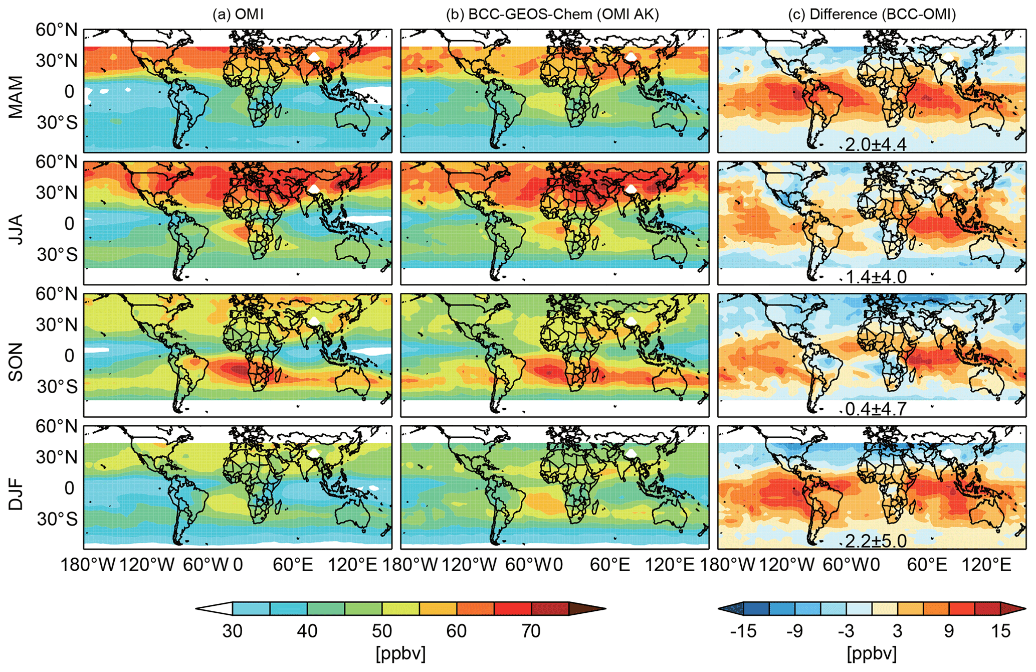
Figure 4 Spatial and seasonal distributions of tropospheric ozone at 700–400 hPa from (a) OMI satellite observations, (b) BCC-GEOS-Chem v1.0 model results (with OMI averaging kernels applied), and (c) differences between the two (model results minus observations) with the seasonal mean differences (± standard deviations) shown inset. Values are 3-year averages over 2012–2014.

The model captures well the main features of tropospheric ozone distribution and seasonal variation. Both satellite observations and BCC-GEOS-Chem v1.0 model results show high mid-tropospheric ozone levels over the northern midlatitudes in boreal spring due to stronger stratospheric influences and in summer due to higher photochemical production and over the Atlantic and southern Africa during boreal autumn driven by strong biomass burning emissions (Fig. 2), lightning NOx, and dynamical processes (e.g., Sauvage et al., 2007). The spatial patterns of observed and simulated tropospheric ozone values are highly correlated with correlation coefficients (r) of 0.79–0.93. BCC-GEOS-Chem v1.0 shows small global seasonal mean biases of 0.4–2.2 ppbv relative to OMI observations, which is comparable to the biases of 0.1–2.7 ppbv for G5NR-Chem (NASA GEOS-ESM with GEOS-Chem v10-01 as an online chemical module) in a similar period (Hu et al., 2018). We find that BCC-GEOS-Chem v1.0 tends to overestimate tropospheric ozone levels over tropical oceans by 3–12 ppbv and underestimate ozone over the northern midlatitudes by 3–9 ppbv, similar to the patterns simulated by the classic GEOS-Chem and G5NR-Chem models (Hu et al., 2017, 2018).

Comparisons with global ozonesonde observations further demonstrate that BCC-GEOS-Chem v1.0 has no significant biases in the tropospheric ozone simulation. As shown in Fig. 5, the model reproduces well the observed annual mean ozone vertical structures, e.g., the slow increase in ozone with increasing altitude in the troposphere, and the sharp ozone gradient near and above the tropopause. Figure 6 compares seasonal variations of ozone concentrations in different regions at three tropospheric levels (800, 500, and 300 hPa). Overall, the model reproduces the ozone annual cycles driven by different chemical and dynamical processes. The model captures the springtime and summertime ozone peaks at the northern midlatitudes (Japan, United States, Europe, Canada) (r=0.53–0.94 for different layers) but only fairly reproduces the annual ozone cycle in the Southern Hemisphere (SH) and the tropics. Mean model biases at the three layers are mostly within 10 ppbv with small low biases over the northern midlatitudes (−6.0 to −0.6 ppbv) and high biases over the tropics in the lower and middle troposphere (e.g., about 10 ppbv at 800 hPa over the SH tropics), which is consistent with the comparison with satellite observations (Fig. 4). We find that the model has large low ozone bias in the upper troposphere (300 hPa) particularly over the northern polar regions ($\sim -\mathrm{30}$ ppbv). The underestimation extends to the stratosphere globally except for the extratropical Southern Hemisphere (Fig. 5). These negative model biases are likely due to the use of a simplified stratospheric ozone scheme and/or errors in the modeling dynamics of ozone exchange between the stratosphere and the troposphere, as will be discussed later, or the low model vertical resolution (26 layers).

Figure 5 Comparisons of BCC-GEOS-Chem v1.0 simulated annual mean ozone vertical profiles to ozonesonde observations averaged over the 10 regions (Fig. 3) from south to north. Black horizontal bars are the standard deviations of observations. Numbers of available sites and records for each region in 2012–2014 are given inset.

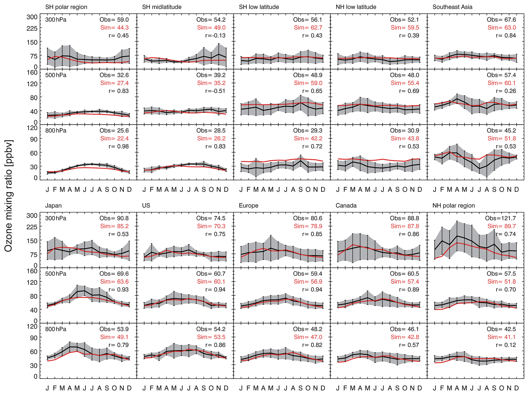
Figure 6 Seasonal variations of ozonesonde observed (black lines) and model simulated (red lines) ozone at three pressure levels (300, 500, and 800 hPa) averaged over the 10 regions (Fig.3). Vertical black bars and gray shadings are the standard deviations of observations. The annual means of observed and simulated ozone concentrations and their correlation coefficients are shown inset. Values are 3-year averages over 2012–2014.

Figure 7 compares the simulated ground-level ozone with more than 300 rural/remote sites (defined by a number of metrics including population density and nighttime lights data; Schultz et al., 2017b) around the world from the TOAR database. We average all observations within the same model grid square for statistical analyses, a recommended way for evaluating coarse-resolution chemical models (Cooper et al., 2020). BCC-GEOS-Chem v1.0 captures the spatial and seasonal distributions of global ground-level ozone with r ranging from 0.53 to 0.59 (N=154). The annual mean model biases are 4.9 ppbv (15 %) for all observations with a larger high bias in the June–July–August period (11.0 ppbv, 32 %). The inclusion of urban and suburban sites slightly decreases the spatial correlations (r=0.34–0.60, N=292) and enlarges the annual mean high bias (10.2 ppbv). We find again that the high biases are more prominent in the tropics (e.g., coastal sites in the western Pacific and Indonesia) and in summer. Although the above comparison is heavily weighted toward the United States, Europe, Japan, and South Korea due to the quantity of observations in these regions, our results demonstrate the overall good performance of BCC-GEOS-Chem v1.0 in simulating ground-level ozone at least for rural and remote regions.

Figure 7 Spatial and seasonal distributions of observed and simulated surface ozone mixing ratios for 2012–2014. The model results (b) are compared to observations at rural/remote sites from the TOAR dataset (a). Observations are averaged to the same model grid. Seasonal mean values for observations and model results, their spatial correlation coefficients (r), and the number of co-sampled grids (N) are shown inset.

3.3 Tropospheric ozone and OH budgets in BCC-GEOS-Chem v1.0

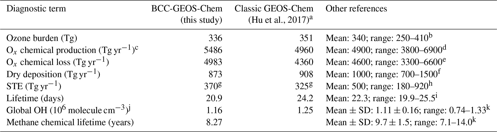
We then diagnose the global tropospheric ozone burden and its driving terms (Table 4 and Fig. 8). BCC-GEOS-Chem v1.0 estimates the global tropospheric ozone burden to be 336.0 Tg averaged over 2012–2014. This is consistent with the results from the classic offline GEOS-Chem CTM and the G5NR-Chem (∼350 Tg) with an earlier version (v10-01) of GEOS-Chem as the chemical module (Hu et al., 2017, 2018), and it is also in agreement with the recent model assessments of 49 models (320–370 Tg; Young et al., 2018). We divide the global tropospheric ozone burden into different regions following Young et al. (2013), as shown in Fig. 8a and b. We find that the overall distributions of ozone burden are consistent with the ensemble of 15 models from the Atmospheric Chemistry and Climate Model Intercomparison Project (ACCMIP) (Young et al., 2013). The main discrepancy between BCC-GEOS-Chem v1.0 and ACCMIP occurs within 30^∘ S–30^∘ N. ACCMIP results show that ozone over 30^∘ S–30^∘ N and below 250 hPa accounts for 36.9 % of the global tropospheric ozone burden, while BCC-GEOS-Chem v1.0 shows a higher proportion (48.5 %). While the ozone overestimation of BCC-GEOS-Chem v1.0 over 30^∘ S–30^∘ N is also seen from the comparisons to observations as discussed previously, the discrepancy between our results and the ACCMIP model ensemble mean is also likely due to the different simulation year (2000 conditions for ACCMIP versus 2012–2014 for BCC-GEOS-Chem v1.0). Zhang et al. (2016) showed that the equatorward redistribution of anthropogenic emissions significantly increased the global tropospheric ozone burden from 1980 to 2010 with the largest enhancements over the tropics. BCC-GEOS-Chem v1.0 underestimates the proportion of ozone burden in the upper troposphere (5.1 %–10.9 %) compared to the ACCMIP results (6.4 %–15.2 %), again likely reflecting the model limitation in simulating stratosphere ozone and/or its exchange with the troposphere.

Table 4 Global budget of tropospheric ozone diagnosed in BCC-GEOS-Chem v1.0 and comparison with other studies.

^a From Table 2 in Hu et al. (2017). The GEOS-Chem version is v10-01. ^b From Fig. 3 in Young et al. (2018), 49 models for year 2000 conditions. ^c Budget is for the odd oxygen family, including O₃, NO₂, NO_y, several organic nitrates, and bromine species to account for the rapid cycling among O_x constituents. Ozone accounts for more than 95 % of the total O_x. ^d From Fig. 3 in Young et al. (2018), 33 models for year 2000 conditions. ^e From Fig. 3 in Young et al. (2018), 32 models for year 2000 conditions. ^f From Fig. 3 in Young et al. (2018), 33 models for year 2000 conditions. ^g Estimated from the residual of mass balance between tropospheric chemical production, chemical loss, and deposition. ^h From Fig. 3 in Young et al. (2018), 34 models for year 2000 conditions. ⁱ From Table 2 in Young et al. (2013), 6 models for year 2000 conditions. ^j Global annual mean air mass weighted OH concentration in the troposphere. ^k From Table 1 in Naik et al. (2013), 16 models for year 2000 conditions. SD stands for standard deviation.

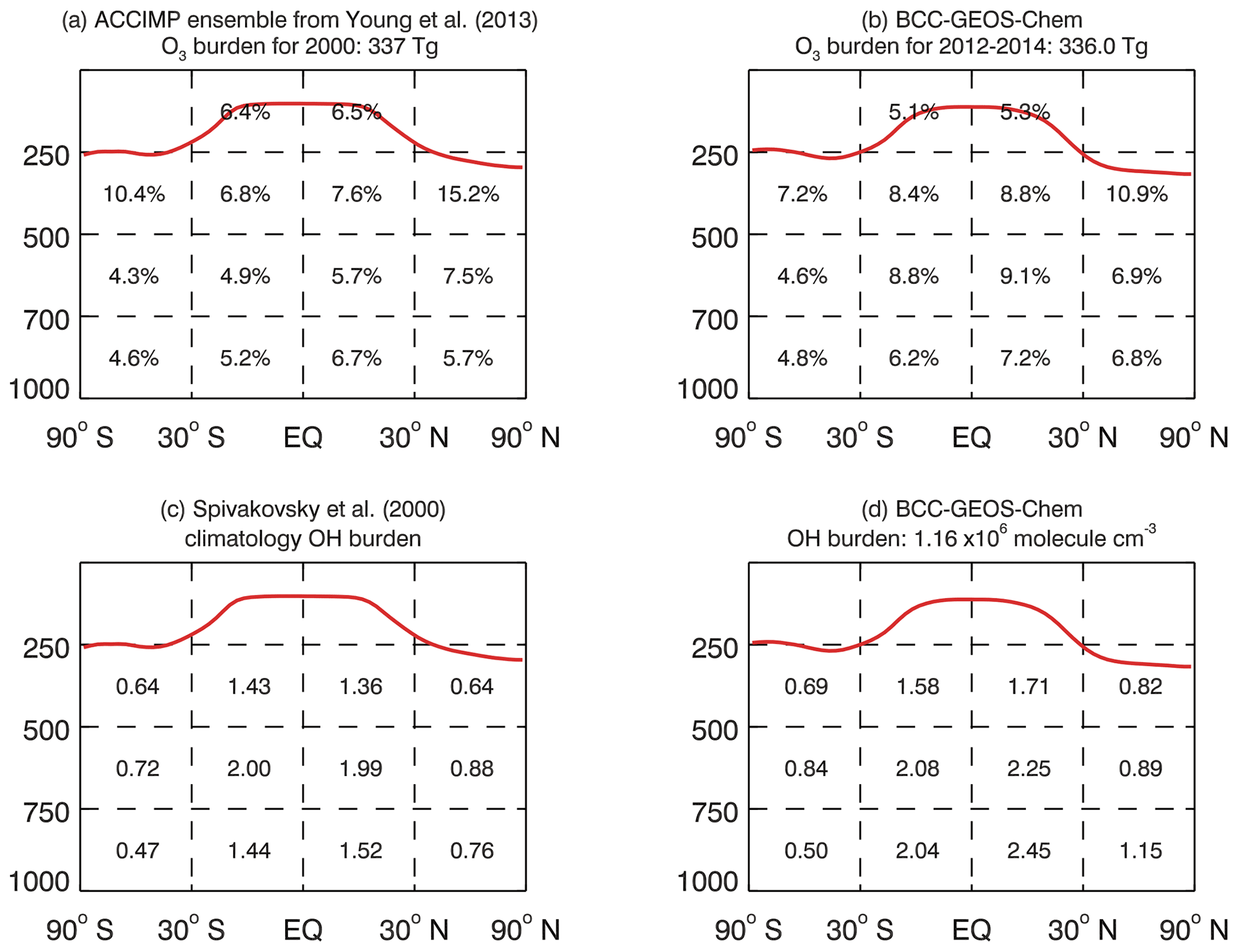
Figure 8 Zonal and vertical distributions of the tropospheric ozone burden and OH concentrations. For comparison, panel (a) shows tropospheric ozone burden in the year 2000 from Young et al. (2013) based on 15 ACCMIP models, and panel (c) shows the climatological tropospheric OH burden reported by Spivakovsky et al. (2000) and summarized by Emmons et al. (2010). Panel (b) and (d) show corresponding results from BCC-GEOS-Chem v1.0 averaged over 2012–2014. The red lines in (a) and (c) denote the tropopause derived from the National Centers for Environmental Prediction (NCEP) reanalysis, and those in (b) and (d) are from BCC-GEOS-Chem v1.0.

We find that the global tropospheric mean OH concentration in BCC-GEOS-Chem v1.0 is 1.16×10⁶ molecule cm⁻³, close to the offline GEOS-Chem v10-01 (1.25×10⁶ molecule cm⁻³; Hu et al., 2018) and well within the range of 16 ACCMIP models ($\mathrm{1.11}\pm \mathrm{0.16}\times {\mathrm{10}}^{\mathrm{6}}$ molecule cm⁻³; Naik et al., 2013). Figure 8c and d compare the distribution of simulated OH concentrations with the climatology derived from previous studies (Spivakovsky et al., 2000; Emmons et al., 2010). We find that the model shows notable high bias in the lower troposphere (below 750 hPa) particularly in the tropics (2.04 to 2.45 molecule cm⁻³ in BCC-GEOS-Chem v1.0 compared to 1.44 to 1.52 molecule cm⁻³ in Spivakovsky et al., 2000). Discrepancies in modeling climate and concentrations of methane, ozone, NO_x, and CO can all contribute to the OH bias in climate–chemistry models (Nicely et al., 2020). We calculate the methane chemical lifetime against OH loss to be 8.3 years in BCC-GEOS-Chem v1.0, which falls in the low end of the range reported from ACCMIP multimodel assessments (9.7±1.5 years) (Naik et al., 2013).

We now diagnose the budget of global tropospheric ozone in BCC-GEOS-Chem v1.0. Following the classic GEOS-Chem, BCC-GEOS-Chem v1.0 diagnoses the chemical production and loss of the odd oxygen family (O_x, including O₃, NO₂, NO_y, several organic nitrates, and bromine species) to account for the rapid cycling among O_x constituents. Ozone accounts for more than 95 % of the total O_x (Hu et al., 2017). The global annual ozone chemical production and loss are 5486 and 4983 Tg, respectively (Table 4); both are higher than the classic GEOS-Chem (Hu et al., 2017) and fall in the high quartile of multimodel assessments (Young et al., 2018). The high tropospheric ozone production is due at least in part to the high precursor emissions used in this study particularly for NO_x emissions. The model shows strong chemical production over northern midlatitude continents in summertime and large chemical loss over the tropical oceans driven by high water vapor content (figure not shown).

The global annual mean ozone dry deposition flux diagnosed in BCC-GEOS-Chem v1.0 is 873 Tg averaged over 2012–2014. It is consistent with recent reviews by Hardacre et al. (2015) and Young et al. (2018) (700–1500 Tg from 33 model estimates). Figure 9 presents the global ozone dry deposition velocity and flux for January and July 2012–2014. Both hemispheres show larger ozone dry deposition velocities in summer than winter due to stronger atmospheric turbulence and larger vegetation cover. A large ozone dry deposition velocity (>0.5 cm s⁻¹) can be seen over the tropical continents, while over the oceans and glaciers ozone dry deposition is very weak.

Figure 9 Monthly mean model diagnosed ozone deposition velocities (cm s⁻¹) and fluxes (kg m⁻²) in January (a, b) and July (c, d).

We then diagnose the annual amount of ozone stratosphere–troposphere exchange (STE) of 370 Tg as the residual of mass balance between tropospheric chemical production, chemical loss, and deposition as previous studies did (Lamarque et al., 2012; Hu et al., 2017). This value is lower than most of the other model estimates (400–680 Tg; Young et al., 2018). The low STE in BCC-GEOS-Chem v1.0 appears to be the main factor causing ozone underestimates in the upper troposphere, as seen above. This may reflect a number of model limitations, for example, the representation of stratospheric chemistry, inadequate STE due to model meteorology (e.g., biases in wind and tropopause), and the low model vertical resolution. Given the tropospheric ozone burden and its loss to chemistry and deposition, we derive the lifetime of tropospheric ozone of 20.9 d, which is consistent with the multimodel estimates (Young et al., 2013).

Figure 10 Spatial distributions of satellite observed (top panels) and model simulated (bottom panels) annual mean (a) CO mixing ratio at 700 hPa, (b) tropospheric NO₂ column, (c) SO₂ column in the planetary boundary layer, and (d) tropospheric CH₂O column. Values are 3-year averages over 2012–2014.

3.4 Evaluation of other atmospheric constituents

Figure 10 compares the spatial distributions of annual mean simulated CO, NO₂, SO₂, and CH₂O with satellite observations. We evaluate CO at 700 hPa where the MOPITT satellite has generally high sensitivity (Emmons et al., 2004; Pfister et al., 2005) and apply averaging kernels to smooth the modeled CO. As shown in Fig. 10, BCC-GEOS-Chem v1.0 reproduces the high CO levels over the northern midlatitudes driven by higher anthropogenic sources and over central Africa driven by biomass burning emissions (spatial correlation coefficient r=0.92) with some overestimates. It also captures the observed hot spots of tropospheric NO₂ (r=0.87) and PBL SO₂ (r=0.32) columns over East Asia that generally follow the distribution of anthropogenic sources. The sharp land–ocean gradients for both tracers reflect their short chemical lifetime. We find low biases in the modeled PBL SO₂ especially over the volcanic eruption regions (e.g., central Africa) but high biases in the industrialized regions such as East Asia, a pattern consistent with previous comparisons between the OMI and GEOS-Chem PBL SO₂ columns, which may reflect inappropriate ship and volcanic emissions in the model (Lee et al., 2009) and/or the model bias in the PBL height. High levels of the tropospheric CH₂O column are simulated over the Amazon, central Africa, tropical Asia, and the southeastern United States, typical regions where CH₂O is oxidized from large biogenic emissions of volatile organic compounds (VOCs) (r=0.67), but the model shows notable overestimates. Previous studies (Zhu et al., 2016, 2020) showed that satellite CH₂O retrievals are low biased by 20 %–51 % compared to aircraft measurements, which would partly explain the model bias. Future assessments are required to correct the biases of these gaseous pollutants.

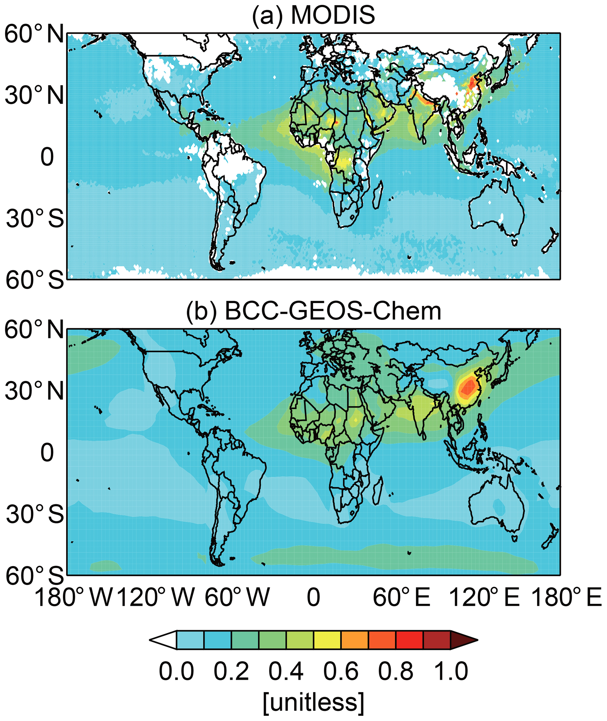
Figure 11 Spatial distributions of annual mean aerosol optical depth (AOD) at 550 nm from (a) MODIS satellite observations and (b) BCC-GEOS-Chem v1.0 averaged over 2012–2014.

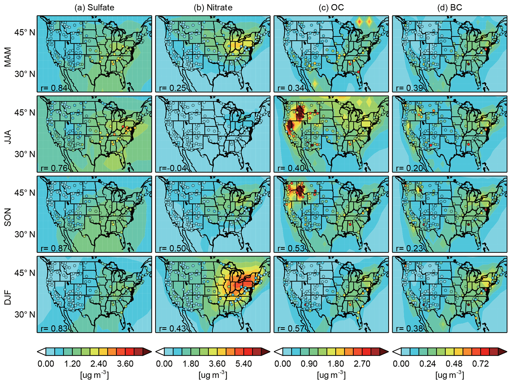
Figure 12 Spatial and seasonal distributions of simulated surface concentrations (contours) of (a) aerosol sulfate, (b) nitrate, (c) organic carbon, and (d) black carbon compared with observations from the United States IMPROVE network (circles) for 2012–2014. Correlation coefficients between observations and model results sampled at the site locations are shown inset.

We evaluate model simulated AOD at 550 nm with the MODIS AOD observations in Fig. 11. High AOD values over East Asia due to high anthropogenic emissions and over Africa and the adjacent oceans due to dust emissions are shown in both MODIS observations and BCC-GEOS-Chem v1.0, although the model tends to underestimate the observed hot spots likely due to the coarse model resolution. Figure 12 further shows the comparison of simulated surface aerosol components (sulfate, nitrate, OC, and BC) with the observations from the IMPROVE network over the United States. The model fairly reproduces the spatial and seasonal patterns for all analyzed aerosol components, e.g., high sulfate and nitrate concentrations over the eastern United States. Among all the components, the simulation of sulfate in the United States shows best agreement with biases of −10 %–20 % and spatial correlation coefficients of 0.76–0.87 over model grids covering the measurement sites (N=77). The model also captures the high summertime OC and BC concentrations in the midwestern United States driven by active wildfire activities (r=0.20–0.57 for different seasons). However, the model shows high biases in wintertime nitrate in the eastern United States as found in previous GEOS-Chem evaluations (Zhang et al., 2012).

4 Summary and future plans

This study describes the framework and evaluation of the new global atmospheric chemistry general circulation model BCC-GEOS-Chem v1.0. The development of the BCC-GEOS-Chem v1.0 takes advantage of the grid-independent structure of the GEOS-Chem chemical module, which allows the exact same GEOS-Chem chemistry and deposition algorithms to be performed on any external grid and supported by MPI (Message Passing Interface). BCC-GEOS-Chem v1.0 includes interactive atmospheric and land modules. It simulates the evolution of atmospheric chemical interactive constituents through a detailed mechanism of HO_x–NO_x–VOCs–ozone–bromine–aerosol tropospheric chemistry, as well as online wet and dry deposition schemes. The model also implements a number of climate-sensitive natural emissions such as biogenic VOCs and lightning NO. We conduct a 3-year (2012–2014) model simulation with year-specific CMIP6 anthropogenic and biomass burning emissions. We evaluate the model with a focus on tropospheric ozone using surface, ozonesonde, and satellite observations. We show that BCC-GEOS-Chem v1.0 can capture well the spatial distributions (r=0.79–0.93 with OMI satellite observations of ozone at 700–400 hPa) and seasonal cycles of tropospheric ozone. The model shows no significant biases in the lower and middle tropospheric ozone compared to satellite observations (0.4–2.2 ppbv at 700–400 hPa), ozonesonde (within 10 ppbv at 800, 500, and 300 hPa except for the polar upper troposphere), and surface measurements (4.9 ppbv). We calculate a global tropospheric ozone burden of 336 Tg yr⁻¹ and OH burden of 1.16×10⁶ molecule cm⁻³; both are well within the ranges reported by previous studies. Regionally, the model shows notable high biases in ozone over the tropics and low ozone biases in the upper troposphere. Model diagnostics show that BCC-GEOS-Chem v1.0 has higher tropospheric ozone chemical production and loss compared to the classic GEOS-Chem but still falls in the range of previous estimates. Comparisons of other air pollutants including NO₂, SO₂, CO, CH₂O, and aerosols show reasonable agreements with biases likely due to uncertainties in emissions.

The development of BCC-GEOS-Chem v1.0 for online atmospheric chemistry simulations represents an important step in the development of fully coupled earth system models in China. There are still several limitations in this version that should be addressed in future model development. The current version of BCC-GEOS-Chem does not include a full stratospheric chemistry mechanism, which is important for accurately modeling the evolution of ozone and its climate influences (Lu et al., 2019a). We plan to implement the unified tropospheric–stratospheric chemistry extension (UCX) (Eastham et al., 2014), which is now the “standard” mechanism for GEOS-Chem chemistry, into the next version of BCC-GEOS-Chem. Diagnosing radiative transfer and aerosol–cloud interactions will be the next priority for model evaluation, and it can take advantage of the GEOS-Chem aerosol microphysics module – the TwO-Moment Aerosol Sectional (TOMAS) module (Kodros and Pierce, 2017) – or Advanced Particle Microphysics (APM) module (Yu and Luo, 2009). Updates of emissions (e.g., application of new or regional anthropogenic emission inventories) could be merged to BCC-GEOS-Chem with the future implementation of the GEOS-Chem emission module (Harvard–NASA Emissions Component, HEMCO) (Keller et al., 2014). BCC-GEOS-Chem is ready to be updated to a higher horizontal and vertical resolution of T106 (about 110 km, 46 layers up to 1.5 hPa) or T266 (about 45 km, 56 layers up to 0.09 hPa) with recent the BCC-CSM-MR and BCC-CSM-HR (Wu et al., 2019), which will enable applications on air quality prediction in the future.