the Creative Commons Attribution 4.0 License.
the Creative Commons Attribution 4.0 License.
 | 06 Aug 2020
HighResMIP versions of EC-Earth: EC-Earth3P and EC-Earth3P-HR – description, model computational performance and basic validation
Mario Acosta
Rena Bakhshi
Pierre-Antoine Bretonnière
Louis-Philippe Caron
Miguel Castrillo
Susanna Corti
Paolo Davini
Eleftheria Exarchou
Federico Fabiano
Uwe Fladrich
Ramon Fuentes Franco
Javier García-Serrano
Jost von Hardenberg
Torben Koenigk
Xavier Levine
Virna Loana Meccia
Twan van Noije
Gijs van den Oord
Froila M. Palmeiro
Mario Rodrigo
Yohan Ruprich-Robert
Philippe Le Sager
Etienne Tourigny
Shiyu Wang
Michiel van Weele
Klaus Wyser
A new global high-resolution coupled climate model, EC-Earth3P-HR has been developed by the EC-Earth consortium, with a resolution of approximately 40 km for the atmosphere and 0.25∘ for the ocean, alongside with a standard-resolution version of the model, EC-Earth3P (80 km atmosphere, 1.0∘ ocean). The model forcing and simulations follow the High Resolution Model Intercomparison Project (HighResMIP) protocol. According to this protocol, all simulations are made with both high and standard resolutions. The model has been optimized with respect to scalability, performance, data storage and post-processing. In accordance with the HighResMIP protocol, no specific tuning for the high-resolution version has been applied.
Increasing horizontal resolution does not result in a general reduction of biases and overall improvement of the variability, and deteriorating impacts can be detected for specific regions and phenomena such as some Euro-Atlantic weather regimes, whereas others such as the El Niño–Southern Oscillation show a clear improvement in their spatial structure. The omission of specific tuning might be responsible for this.
The shortness of the spin-up, as prescribed by the HighResMIP protocol, prevented the model from reaching equilibrium. The trend in the control and historical simulations, however, appeared to be similar, resulting in a warming trend, obtained by subtracting the control from the historical simulation, close to the observational one.
- Article
(13655 KB) - Full-text XML
- BibTeX
- EndNote


Recent studies with global high-resolution climate models have demonstrated the added value of enhanced horizontal atmospheric and oceanic resolution compared to the output from models in the Coupled Model Intercomparison Project phases 3 and 5 (CMIP3 and CMIP5) archive. An overview and discussion of those studies has been given in Haarsma et al. (2016) and Roberts et al. (2018). Coordinated global high-resolution experiments were, however, lacking, which induced the launch of the CMIP6-endorsed High Resolution Model Intercomparison Project (HighResMIP). The protocol of HighResMIP is described in detail in Haarsma et al. (2016). Due to the large computational cost that high horizontal resolution implies, the time period for simulations in the HighResMIP protocol ranges from 1950 to 2050. The minimal required atmospheric and oceanic resolution for HighResMIP is about 50 km and 0.25∘, respectively.
EC-Earth is a global coupled climate model (Hazeleger et al., 2010, 2012) that has been developed by a consortium of European institutes consisting, to this day, of 27 research institutes. Simulations with EC-Earth2 contributed to the CMIP5 archive, and numerous studies performed with the EC-Earth model appeared in peer-reviewed literature and contributed to the Fifth Assessment Report (AR5) of the IPCC (Intergovernmental Panel on Climate Change) (IPCC, 2013). EC-Earth is used in a wide range of studies from paleo-research to climate projections, including also seasonal (Bellprat et al., 2016; Prodhomme et al., 2016; Haarsma et al., 2019) and decadal forecasts (Guemas et al., 2013, 2015; Doblas-Reyes et al., 2013; Caron et al., 2014; Solaraju Murali et al., 2019; Koenigk et al., 2013; Koenigk and Brodeau, 2014; Brodeau and Koenigk, 2016).
In preparation for CMIP6, a new version of EC-Earth, namely EC-Earth3, has been developed (Doescher et al., 2020). This has been used for the DECK (Diagnostic, Evaluation and Characterization of Klima) simulations (Eyring et al., 2016) and several CMIP6-endorsed MIPs. The standard resolution of EC-Earth3 is T255 (∼ 80 km) for the atmosphere and 1.0∘ for the ocean, which is too coarse to contribute to HighResMIP. A higher-resolution version of EC-Earth3 therefore had to be developed. In addition, the HighResMIP protocol demands simplified aerosol and land schemes (Haarsma et al., 2016).
In Sect. 2, we will describe the HighResMIP version of EC-Earth3 which has been developed within the European Horizon2020 project PRIMAVERA (Roberts et al., 2018). For a detailed description of the standard CMIP6 version of EC-Earth3 and its technical and scientific performance, we refer to Doescher et al. (2020). High-resolution modeling requires special efforts in scaling, optimization and model performance, which will be discussed in Sect. 3. In Sect. 3, we also discuss the huge amount of data that is produced by a high-resolution climate model that requires an efficient post-processing and storage workflow. A summary of the model results will be given in Sect. 4. In that section, we also discuss the issue that for a high-resolution coupled simulation it is not possible to produce a completely spun-up state that has reached equilibrium due to limited computer resources. As a result, the HighResMIP protocol prescribes that the simulations start from an observed initial state. The drift due to an imbalance of the initial state is then accounted for by performing a control run with constant forcing alongside the transient run.
The model used for HighResMIP is part of the EC-Earth3 family. EC-Earth3 is the successor of EC-Earth2 that was developed for CMIP5 (Hazeleger et al., 2010, 2012; Sterl et al., 2012). Early versions of EC-Earth3 have been used by, e.g., Batté et al. (2015), Davini et al. (2015), and Koenigk and Brodeau (2017). The versions developed for HighResMIP are EC-Earth3P (T255 (∼ 100 km) atmosphere, 1∘ ocean) for standard resolution and EC-Earth3P-HR (T511 (∼ 50 km) atmosphere, 0.25∘ ocean) for high resolution, and will henceforth be referred to as EC-Earth3P(-HR), respectively. In addition, a very-high-resolution version (EC-Earth3P-VHR) (T1279 (∼ 15 km) atmosphere, 0.12∘ ocean) has been developed, and simulations following the HighResMIP protocol are presently being performed but not yet available. Compared to EC-Earth2, EC-Earth3P(-HR) include updated versions of its atmospheric and oceanic model components, as well as a higher horizontal and vertical resolution in the atmosphere.
The atmospheric component of EC-Earth is the Integrated Forecasting System (IFS) model of the European Centre for Medium-Range Weather Forecasts (ECMWF). Based on cycle 36r4 of IFS, it is used at T255 and T511 spectral resolution for EC-Earth3P and EC-Earth3P-HR, respectively. The spectral resolution refers to the highest retained wavenumber in linear triangular truncation. The spectral grid is combined with a reduced Gaussian grid where the nonlinear terms and the physics are computed, with a resolution of N128 for EC-Earth3P, N256 for EC-Earth3-HR and N640 for EC-Earth3P-VHR. Because of the reduced Gaussian grid, the grid box distance is not continuous, with a mean value of 107 km for EC-Earth3P and 54.2 km for EC-Earth3P-HR (Klaver et al., 2020). The number of vertical levels is 91, vertically resolving the middle atmosphere up to 0.1 hPa. The revised land surface hydrology Tiled ECMWF Scheme for Surface Exchanges over Land (H-TESSEL) model is used for the land surface (Balsamo et al., 2009) and is an integral part of IFS; for more details, see Hazeleger et al. (2012).
The ocean component is the Nucleus for European Modelling of the Ocean (NEMO; Madec, 2008). It uses a tripolar grid with poles over northern North America, Siberia and Antarctica and has 75 vertical levels (compared to 42 levels in the CMIP5 model version and standard EC-Earth3). The so-called ORCA1 configuration (with a horizontal resolution of about 1∘) is used in EC-Earth3P, whereas the ORCA025 (resolution of about 0.25∘) is used in EC-Earth3P-HR. The ocean model version is based on NEMO version 3.6 and includes the Louvain-la-Neuve sea-ice model version 3 (LIM3; Vancoppenolle et al., 2012), which is a dynamic–thermodynamic sea-ice model with five ice thickness categories. The atmosphere–land and ocean–sea-ice components are coupled through the OASIS (Ocean, Atmosphere, Sea Ice, Soil) coupler (Valcke and Morel, 2006; Craig et al., 2017).
The NEMO configuration is based on a setup developed by the shared configuration NEMO (ShaCoNEMO) initiative led by Institute Pierre Simon Laplace (IPSL) and adapted to the specific atmosphere coupling used in EC-Earth. The remapping of runoff from the atmospheric grid points to runoff areas on the ocean grid has been re-implemented to be independent of the grid resolution. This was done by introducing an auxiliary model component and relying on the interpolation routines provided by the OASIS coupler. In a similar manner, forcing data for atmosphere-only simulations are passed through a separate model component, which allows to use the same SST and sea-ice forcing data set for different EC-Earth configurations.
IFS and NEMO have the same time steps: 45 min in EC-Earth3P and 15 min in EC-Earth3P-HR. The coupling between IFS and NEMO is 45 min in both configurations.

The CMIP6 protocol requests modeling groups to use specific forcing data sets that are common for all participating models. Table 1 lists the forcings that have been implemented in EC-Earth3P(-HR). Because of the HighResMIP protocol, EC-Earth3P(-HR) differs in several aspects from the model configurations used for the CMIP6 experiments (Doescher et al., 2020).
The stratospheric aerosol forcing in EC-Earth3P(-HR) is handled in a simplified way that neglects the details of the vertical distribution and only takes into account the total aerosol optical depth in the stratosphere which is then evenly distributed across the stratosphere. This approach follows the treatment of stratospheric aerosols as it was used by EC-Earth2 for the CMIP5 experiments yet with the stratospheric aerosol optical depth (AOD) at 500 nm updated to the CMIP6 data set.
A sea surface temperature (SST) and sea-ice forcing data set specially developed for HighResMIP is used for AMIP experiments (Kennedy et al., 2017). The major differences compared to the standard SST forcing data sets for CMIP6 are the higher spatial (0.25∘ vs. 1∘) and temporal (daily vs. monthly) resolution. For the tier 3 HighResMIP SST-forced future AMIP simulations (see Sect. 4.1), an artificially produced data set of SST and sea-ice concentration (SIC) is used, which combines observed statistics and modes of variability with an extrapolated trend (https://esgf-node.llnl.gov/search/input4mips/, last access: 8 March 2019).
The HighResMIP protocol requires the simulations to start from an atmosphere and land initial state from 1950 of the ECMWF ERA-20C (Poli et al., 2016) reanalysis data. Because the soil moisture requires at least 10 years to reach equilibrium with the model atmosphere, a spin-up of 20 years under 1950s forcing has been made before starting the tier 1 simulations.
In agreement with the HighResMIP protocol, the vegetation is prescribed as a present-day climatology that is constant in time.
The climatological present-day vegetation, based on ECMWF ERA-Interim (Dee et al., 2011), and specified as albedos and leaf area index (LAI) from the Moderate-resolution Imaging Spectroradiometer (MODIS) is used throughout all runs. In contrast, the model version for other CMIP6 experiments uses lookup tables to account for changes in land use. In addition, that version is consistent with the CMIP6 forcing data set and not based on ERA-Interim.
Another difference is the version of the pre-industrial aerosols background derived from the TM5 model (Van Noije et al., 2014; Myriokefalitakis et al., 2020, and references therein): version 2 in PRIMAVERA; version 4 in other CMIP6 model configurations using prescribed anthropogenic aerosols. This affects mainly the sea-spray source and in turn the tuning parameters.
New developments in global climate models require special attention in terms of high-performance computing (HPC) due to the demand for increased model resolution, large numbers of experiments and increased complexity of Earth system models (ESMs). EC-Earth3P-HR (and VHR) is a demanding example where efficient use of the resources is mandatory.
The aim of the performance activities for EC-Earth3P-HR is to adapt the configuration to be more parallel, scalable and robust, and to optimize part of the execution when this high-resolution configuration is used. The performance activities are focused on three main challenges: (1) scaling of EC-Earth3P-HR to evaluate the ideal number of processes for this configuration, (2) analyses of the main bottlenecks of EC-Earth3P-HR and (3) new optimizations for EC-Earth3P-HR.
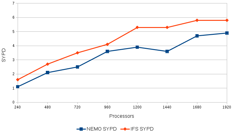
Figure 1NEMO (red) and IFS (blue) scalability in EC-Earth3P-HR. The throughput is expressed in simulated years per day (SYPD) of wall-clock time. The tests have been performed on the MareNostrum4 computer at the Barcelona Computing Centre with full output and samples of five 1-month runs for each processor combination, the average of which is shown in the figure. The horizontal axis corresponds to the number of cores used.
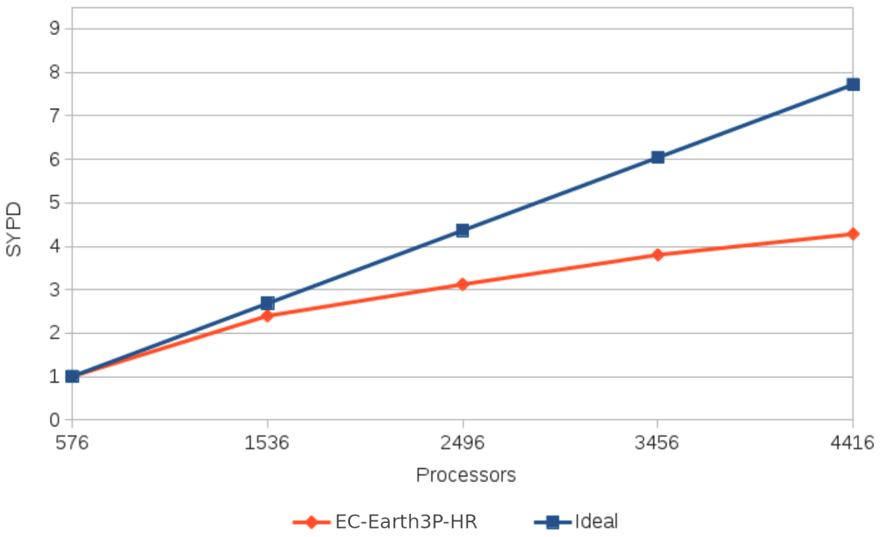
Figure 2As Fig. 1 but for the scalability of the fully coupled EC-Earth3P-HR. The blue diagonal indicates perfect scalability.
3.1 Scalability
The results of the scalability analyses of the atmosphere (IFS) and ocean (NEMO) components of EC-Earth3P-HR are shown in Fig. 1 and for the fully coupled model in Fig. 2. Acosta et al. (2016) showed that, while for coupled application the load balance between components has to be taken into account in the scalability process, the process needs to start with a scalability analysis of each individual component. Moreover, the user could experience that the speeding up of one component (e.g., the reduction of the execution time of IFS) does not reduce the execution time of the coupled application. This could be because there is one synchronization point at the end each coupled time step where both components exchange fields. If the other non-optimized components are slower, a load rebalance will be required. The final choice depends on the specific problem, where either time or energy can be minimized. In Sect. 3.2, we describe how the optimal load balance between the two components, where NEMO is the slowest component, was achieved (Acosta et al., 2016).
3.2 Bottlenecks
For the performance analysis, the individual model components (IFS, NEMO and OASIS) are benchmarked and analyzed using a methodology based on extracting traces from real executions. These traces are displayed using the PARAVER (PARAllel Visualization and Events Representation) software and processed to discover possible bottlenecks (Acosta et al., 2016). Eliminating these bottlenecks not only involves an adjustment of the model configuration and a balance of the number of cores devoted to each one of its components but also modifications of the code itself and work on the parallel programming model adopted in the different components.
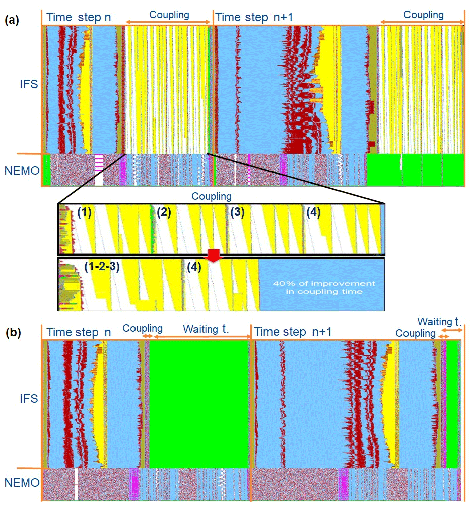
Figure 3(a) PARAVER view of the NEMO and IFS components in an EC-Earth3P-HR model execution for two time steps including the coupling process. The horizontal lines give the behavior of the different processes (1 to 512 for IFS and 513 to 536 for NEMO) as a function of time. Each color corresponds to a different MPI communication function. See text for explanation. Panel (b) is the same as (a) but when optimization options “opt” and “gathering” for coupling are activated.
The first step of a performance analysis consists in analyzing parallel programming model codes using targeted performance tools. Figure 3a illustrates an example of the performance tool's output from one single EC-Earth3P-HR model execution as provided by the PARAVER tool, focusing only on its two main components: NEMO and IFS. This figure is very useful for determining the communications within the model and identify sources of bottlenecks, especially those resulting from communication between components. It displays the communication pattern as a function of time. The vertical axis corresponds to the different processes executing the model, the top part for IFS and the lower part for NEMO. The different colors correspond to different MPI communication functions, except the light blue, which corresponds to no communication. Red, yellow and purple colors are related to MPI communications. The green color represents the waiting time needed to synchronize the coupled model for the next time step, which means an unloaded balance in the execution. In summary, light blue areas are pure computation and should be maximized. On the other hand, yellow, red and purple are representing overhead from parallel computation and should be minimized if possible. Additionally, green areas are preferably to be also reduced, for example, increasing the number of parallel resources of the slowest component, but no optimizations are needed. From this analysis, several things can be concluded related to the overhead from parallel computation:
-
Figure 3 shows the coupling cost from a computational point of view, including one regular time step of IFS and NEMO and one time step including the coupling process. In the top part of Fig. 3a, we notice that during the first half of the first time step, the IFS component model reserves most of its processors for execution (512 processes). To simplify, it can be said that the first half of the time step has less MPI communication, with more computation-only regions, while the second half of the time step is primarily about broadcasting messages (yellow and white color block), which corresponds to the coupling computation and to send/receive files from the atmospheric to the ocean model. These calculations impact the scalability of the code dramatically. This configuration increases the overhead when more and more processes are used and represents more than 50 % of time execution when 1024 processes are used. The coupling process can be analyzed in detail in Fig. 3a (coupling zoom, top image), where the same pattern of communications is repeated four times. This occurs because the different fields from IFS to NEMO are sent in three different groups, followed by an additional group of fields sent from IFS to the runoff mapper component. The communication of three different groups of fields to the same component is not taking advantage of the bandwidth of the network, thus increasing the overhead produced by MPI communications. However, these three groups are using the same interpolation method and they could be gathered into the same group.
-
From other parts of the application (not shown in the figure), we also notice the expensive cost of the IFS output process for each time step. A master process gathers the data from all MPI subdomains and prints the complete outputs at a regular time interval of 3–6 h. During this process, the rest of processes are waiting for this step to be completed. Due to the large data volumes, this sequential process is very costly, increasing the execution time of IFS by about 30 % when outputs are required, compared to the regular time step of IFS (without output).
-
The bottom part of Fig. 3a shows that the communication in NEMO is not very effective and that a large part of it is devoted to global communications, which appear in purple. Those communications belong to the horizontal diffusion routine, inside the ice model (LIM3) used in NEMO. The high frequency of communications in this routine prevented the model from scaling. More information about MPI overhead of NEMO can be found in Tintó et al. (2019).
-
Due to the domain decomposition used by NEMO, some of the MPI processes, which are used to run part of the ocean domain in parallel, were computing without use. This is because domain decomposition is done on a regular grid and a mask is used to discriminate between land and sea points. The mask creates subdomains of land points whose calculations are not used. This is illustrated in Fig. 4, which shows a particular case in which 12 % of the depicted subdomains do not contain any sea point.
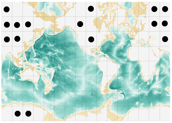
Figure 4Domain decomposition of a tripolar grid of the ORCA family with a resolution of 1.0∘ into 128 subdomains (16×8). Subdomains marked with a black dot do not contain any ocean grid point.
3.3 New optimizations for the specific configuration
According to the profiling analysis done, different optimizations were implemented to improve the computational efficiency of the model:
-
The optimization (“opt”) option of OASIS3-MCT was used. This activates an optimized global conservation transformation. Using this option, the coupling time from IFS to NEMO is reduced by 90 % for EC-Earth3P-HR. This is because all-to-one/one-to-all MPI communications are replaced by global communications (gather/scatter and reduction) and the coupling calculations are done by all the IFS processes instead of only the IFS master process.
Another functionality of OASIS consists in gathering all fields sent from IFS to NEMO in a single group (Acosta et al., 2016). Coupling field gathering, an option offered by OASIS3-MCT, can be used to optimize coupling exchanges between components. The results show that gathering all the fields that use similar coupling transformations reduces the coupling overhead. This happens because OASIS3-MCT is able to communicate and interpolate all of the fields gathered at the same time. Figure 3a (coupling zoom, bottom image) proves that the collection of the first three groups reduces the communication patterns from four to two, where the execution time of this part is reduced significantly (40 %).
Figure 3b shows the execution when “opt” and “gathering” options are used, with the 90 % reduction in coupling time clearly visible (large green section). In the case of the first time step in the trace, the coupling time is replaced by waiting time, since NEMO is finishing its time step and both components have to exchange fields at the end of the time step.
-
For the output problem, the integration of XIOS as the I/O server for all components of EC-Earth can increase performance dramatically. XIOS is already used for the ocean component NEMO and the I/O server receiving also all the data from IFS processes and doing the output work in parallel and in an asynchronous way is the best solution to remove the sequential process when an IFS master process is required to do this work. This is being developed and will be included in the next version of EC-Earth.
-
Based on the performance analysis, the amount of MPI communications can be reduced (Tintó et al., 2019), achieving a significant improvement in the maximum model throughput. In the case of EC-Earth3P-HR, this translated into a reduction of 46 % in the final execution time.
-
Using the tool ELPiN (Exclude Land Processes in NEMO), the optimal domain decomposition for NEMO has been implemented (Tintó et al., 2017), with computation of only ocean subdomains and finding the most efficient number of MPI processes. This substantially improves both the throughput and the efficiency (in the case of 2048 processor cores, 41 % faster using 25 % less resources). The increase in throughput was due to fewer computations and, related to that, fewer communications. In addition, ELPiN allows for the optimal use of the available resources in the domain decomposition depending on the shape and overlap of the subdomains.
3.4 Post-processing and data output
At the T511L91 resolution, the HighResMIP data request translates into an unprecedented data volume for EC-Earth. Because the atmosphere component (IFS) is originally a numerical weather prediction (NWP) model, it contains no built-in functionality for time averaging the data stream during the simulation. The model was therefore configured to produce the requested three-dimensional fields (except radiative fluxes on model levels, which cannot be output by the IFS) on a 6-hourly basis and surface fields with 3-hourly frequency. As a consequence, the final daily and monthly averages for instantaneous fields have been produced from sampling at these frequencies, whereas fluxes are accumulated in the IFS at every time step. Vertical interpolation to requested pressure or height levels is performed by the model itself.
For the ocean model, the post-processing is done within NEMO by the XIOS library which can launch multiple processes writing NetCDF files in parallel, alleviating the I/O footprint during the model run. The XIOS configuration XML files were extended to produce as many of the ocean and sea-ice variables as possible.
The combination of the large raw model output volume, the increased complexity of the requested data and the new format of the CMOR tables (Climate Model Output Rewriter, an output format in conformance with all the CMIP standards) required a major revision of the existing post-processing software. This has resulted in the development of the ece2cmor3 package. It is a Python package that uses Climate Data Operators (CDO) (CDO, 2015) bindings for (i) selecting variables and vertical levels, (ii) time averaging (or taking daily extrema), (iii) mapping the spectral and grid-point atmospheric fields to a regular Gaussian grid and (iv) computing derived variables by some arithmetic combination of the original model fields. Finally, ece2cmor3 uses the PCMDI CMOR library for the production of NetCDF files with the appropriate format and metadata. The latter is the only supported step for the ocean output.
To speed up the atmosphere post-processing, the tool can run multiple CDO commands in parallel for various requested variables. Furthermore, we optimized the ordering of operations, performing the expensive spectral transforms on time-averaged fields wherever possible. We also point out that the entire procedure is driven by the data request; i.e., all post-processing operations are set up by parsing the CMOR tables and a single dictionary relating EC-Earth variables and CMOR variables. This should make the software easy to maintain with respect to changes in the data request and hence useful for future CMIP6 experiments.
4.1 Outline of HighResMIP protocol
The protocol of the HighResMIP simulations consists of tiers 1, 2 and 3 experiments that represent simulations of different priority (1 being the highest, 3 the lowest) and a spin-up procedure. The protocol also excludes specific tuning for the high-resolution version compared to the standard-resolution version. Below, we give a short summary of the protocol. The experiment names in the CMIP6 database are given in italics.
-
Tier 1: forced-atmosphere simulations 1950–2014; highresSST-present. The Tier 1 experiments are atmosphere-only simulations forced using observed sea surface temperature for the period 1950–2014.
-
Tier 2: coupled simulations (1950–2050). The period of the coupled simulations is restricted to 100 years because of the computational burden brought about by the model resolution and the limited computer resources. The period 1950–2050 covers historical multi-decadal variability and near-term climate change. The coupled simulations consist of a spin-up, control, historical and future simulations.
-
Spin-up simulation; spinup-1950. Due to the large computer resources needed, a long spin-up to (near) complete equilibrium is not possible at high resolution. Therefore, as an alternative approach, an analyzed ocean state representative of the 1950s is used as the initial condition for temperature and salinity (Good et al., 2013, EN4 data set). To reduce the large initial drift, a spin-up of about 50 years is made using constant 1950s forcing. The forcing consists of greenhouse gases (GHGs), including O3 and aerosol loading for a 1950s (∼ 10-year mean) climatology. Output from the initial 50-year spin-up is saved to enable analysis of multi-model drift and bias, something that was not possible in previous CMIP exercises, with the potential to better understand the processes causing drift in different models.
-
Control simulation; control-1950. This is the HighResMIP equivalent of the pre-industrial control but uses fixed 1950s forcing. The length of the control simulation should be at least as long as the historical plus future transient simulations. The initial state is obtained from the spin-up simulation.
-
Historical simulation; hist-1950. This is the coupled historical simulation for the period 1950–2014, using the same initial state from the spin-up as the control run.
-
Future simulation; highres-future. This is the coupled scenario simulation 2015–2050, effectively a continuation of the hist-1950 experiment into the future. For the future period, the forcing fields are based on the CMIP6 SSP5-8.5 scenario.
-
-
Tier 3: forced-atmosphere 2015–2050 (2100); highresSST-future. The Tier 3 simulation is an extension of the Tier 1 atmosphere-only simulation to 2050, with an option to continue to 2100. To allow comparison with the coupled integrations, the same scenario forcing as for Tier 2 (SSP5-8.5) is used.
A schematic representation of the HighResMIP simulations is given in Fig. 5.
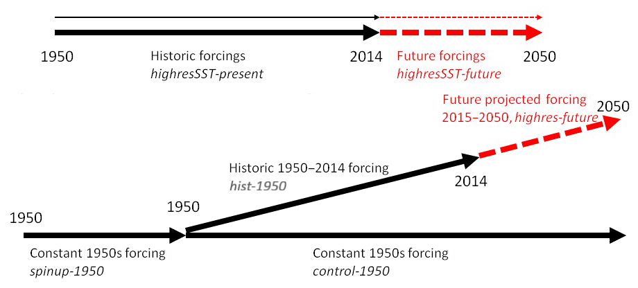
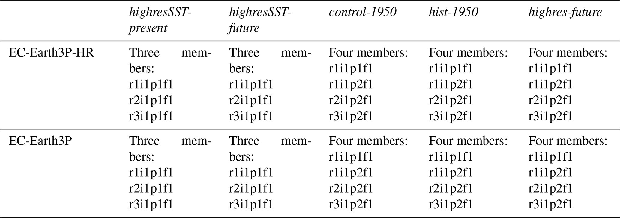
Table 2Overview of the HighResMIP simulations of EC-Earth3P-HR and EC-Earth3P.
4.2 Main results of EC-Earth3P(-HR) HighResMIP simulations
For each of the HighResMIP tiers, more than one simulation was produced. An overview of the simulations is given in Table 2.
The data are stored on the JASMIN server at the Centre for Environmental Data Analysis (CEDA) (https://www.ceda.ac.uk/services/jasmin/, last access: 29 July 2020) and available from Earth System Grid Federation (ESGF). During the PRIMAVERA project, the data were analyzed on the JASMIN server. For the highresSST-present and highresSST-future simulations, the ensemble members were started from perturbed initial states. These were created by adding small random perturbations from a uniform distribution over [, ] degree to the three-dimensional temperature field. For the control-1950 and hist-1950, the end of the spin-up was taken as the initial condition of the first member. For the two extra members, the initial conditions were generated by continuing the spin-up for 5 years after perturbing the fields that are exchanged between atmosphere and ocean. The highres-future members are the continuation of the hist-1950 members.
The Atlantic meridional overturning circulation (AMOC) in the control-1950 of EC-Earth3P had unrealistically low values of less than 10 Sv. It was therefore decided to change the ocean mixing parameters, which improved the AMOC. The main difference compared to the first ensemble member of EC-Earth3P is that the parameterization of the penetration of turbulent kinetic energy (TKE) below the mixed layer due to internal and inertial waves is switched off (nn_etau = 0; Madec and the NEMO team, 2016). The mixing below the mixed layer is an ad hoc parameterization into the TKE scheme (Rodgers et al. 2014) and is meant to account for observed processes that affect the density structure of the ocean's boundary layer. In EC-Earth3P, this penetration of TKE below the mixed layer caused a too-deep surface layer of warm summer water masses in the North Atlantic convection areas, which led to a breakdown of the Labrador Sea convection within a few years and a strongly underestimated AMOC in EC-Earth3P. An additional minor modification compared to ensemble member 1 is an increased tuning parameter rn_lc (= 0.2) in the TKE turbulent closure scheme that directly relates to the vertical velocity profile of the Langmuir cell circulation. Consequently, the Langmuir cell circulation is strengthened.
The new mixing scheme was also applied to EC-Earth3P-HR to ensure the same set of parameters for both versions of EC-Earth3P(-HR). The simulations with the new ocean mixing are denoted with “p2” for the coupled simulations in Table 2. The atmosphere is unchanged, and therefore the atmosphere simulations are denoted as “p1”. Because of the unrealistically low AMOC in EC-Earth3P in the “p1” simulations, we focus on “p2” for the coupled simulations.
Below, we will briefly discuss the mean climate and variability of the highresSST-present, control-1950 and hist-1950 simulations. The main differences between EC-Earth3P and EC-Earth3P-HR will be highlighted. In addition, the spin-up procedure for the coupled simulations, spinup-1950, will be outlined. A more extensive analysis of the HighResMIP simulations will be presented in forthcoming papers.
4.2.1 highresSST-present
The highresSST-present simulations will be compared with ERA5 (Hersbach et al., 2020) (1979–2014), except for precipitation, where Global Precipitation Climatology Project v2.3 (1979–2014) (Adler et al., 2003) data will be used. EC-Earth, GPCP and ERA5 data are regridded to a common grid (N128) before comparison. Seasonal means (December–February (DJF) and June–August (JJA)) will be analyzed. Ensemble mean fields will be displayed.
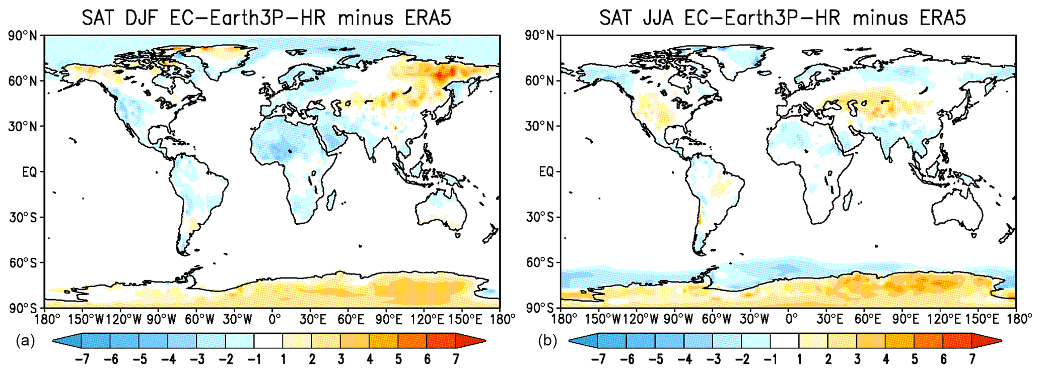
Figure 6SAT: bias (∘C) of EC-Earth3P-HR with respect to ERA5 for the period 1979–2014: (a) DJF and (b) JJA. Global means of SAT for EC-Earth3P-HR are 11.01 (DJF) and 15.85 (JJA), and for ERA5 12.43 (DJF) and 15.95 (JJA). RMSEs of EC-Earth3P-HR with respect to ERA5 are 1.25 (DJF) and 1.06 (JJA).
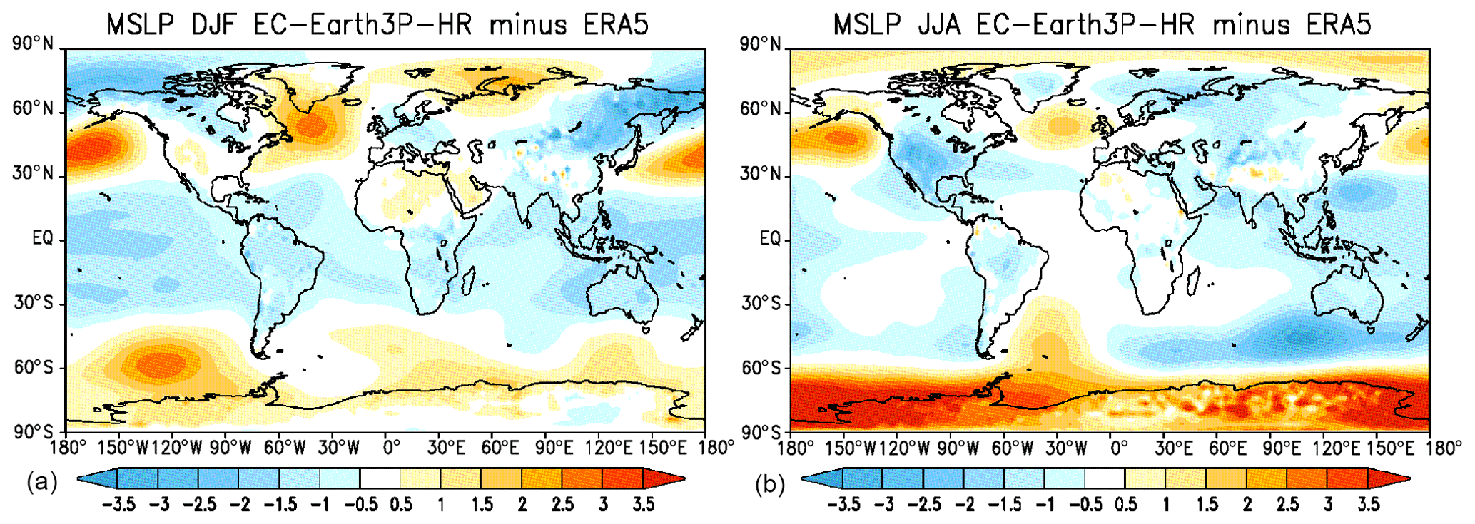
Figure 7MSLP: bias (hPa) of EC-Earth3P-HR with respect to ERA5 for the period 1979–2014: (a) DJF and (b) JJA. Global means of MSLP for EC-Earth3P-HR are 1011.3 (DJF) and 1009.4 (JJA), and for ERA5 1011.53 (DJF) and 1011.24 (JJA). RMSEs of EC-Earth3P-HR with respect to ERA5 are 1.11 (DJF) and 1.27 (JJA).
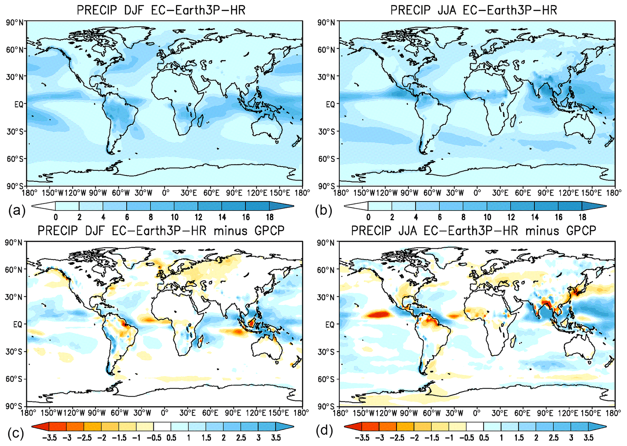
Figure 8Precipitation and bias of EC-Earth3P-HR with respect to GPCP (mm d−1) for the period 1979–2014: (a, c) DJF and (b, d) JJA. Global means of precipitation for EC-Earth3P-HR are 2.91 (DJF) and 3.25 (JJA), and for ERA5 2.70 (DJF) and 2.71 (JJA). RMSEs of EC-Earth3P-HR with respect to ERA5 are 1.06 (DJF) and 1.44 (JJA).
Due to the prescribed SST, the largest surface air temperature (SAT) biases are over the continents (Fig. 6). The largest negative biases are over central Africa for DJF and Alaska in JJA, while the largest positive biases are located over Antarctica in JJA and northeastern Siberia in DJF. Over most areas, EC-Earth3P-HR is slightly too cold. Over most of the tropics, the mean sea level pressure (MSLP) is underestimated, whereas over Antarctica and the surrounding regions of the Southern Ocean it has a strong positive bias (Fig. 7). Also noteworthy is the positive bias south of Greenland during DJF. The largest precipitation errors are seen in the tropics over the warm pool regions in the Pacific and the Atlantic with too much precipitation (Fig. 8). The planetary wave structure of the geopotential height at 500 hPa (Z500) during DJF is well represented, with the exception of the region south of Greenland (Fig. 9), which is consistent with the MSLP bias (Fig. 7a). The physical causes of the aforementioned biases can include a wide range of deficiencies in the parameterizations of cloud physics, land surface and snow, to mention a few. In forthcoming papers, this will be investigated in further detail.
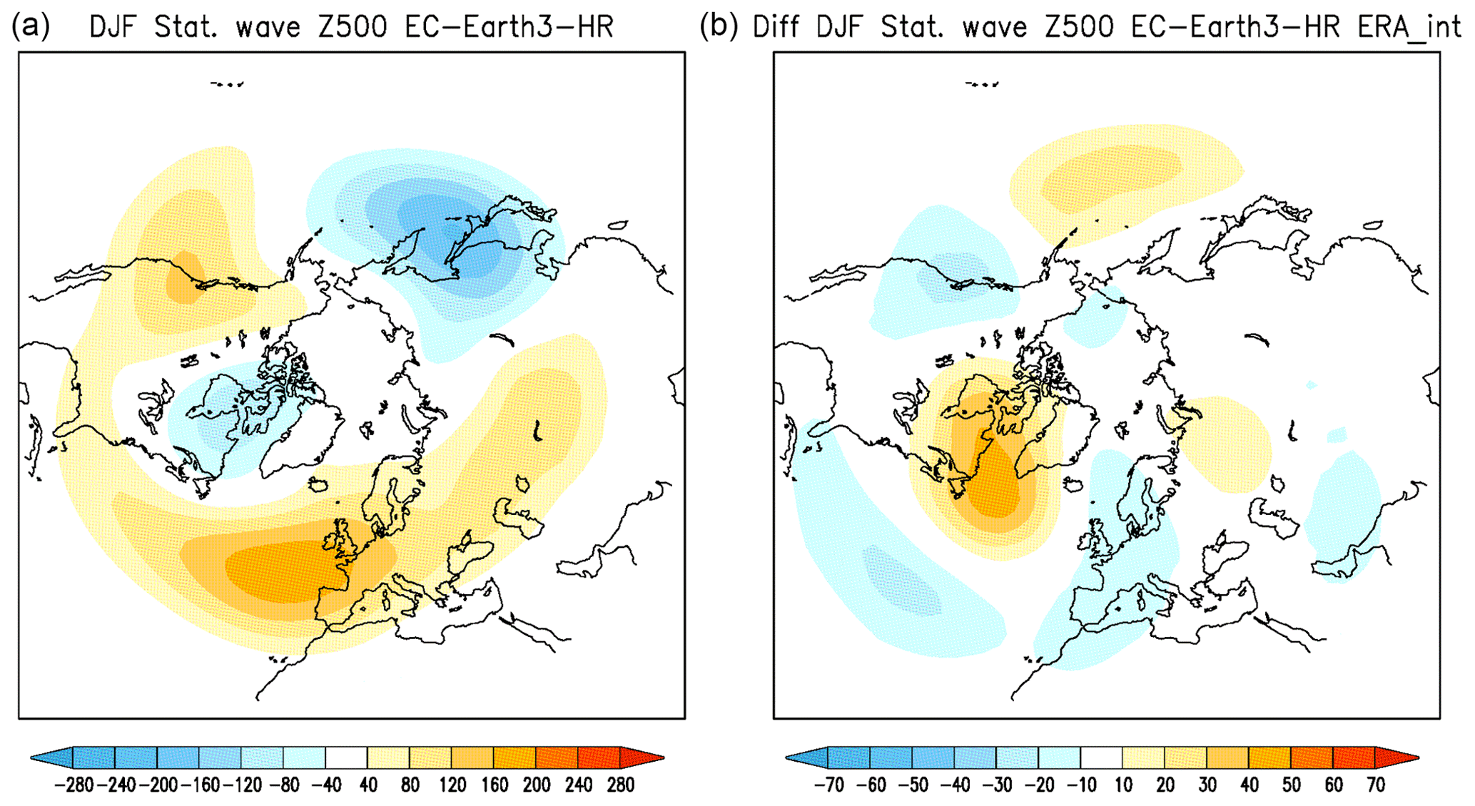
Figure 9(a) Stationary eddy component (departure from zonal mean) of EC-Earth3P-HR of the 500 hPa geopotential height (m) in boreal winter; (b) the difference with ERA5. Note the difference in color scale between the two panels.

Figure 10Differences between EC-Earth3P-HR and EC-Earth3P for SAT (∘C) (a, b), MSLP (hPa) (c, d) and precipitation (mm d−1) (e, f) for DJF (a, c, e) and JJA (b, d, f).
Doubling of the atmospheric horizontal resolution has only a modest impact on the large-scale structures of the main meteorological variables, as illustrated by the global MSLP, SAT and precipitation (Fig. 10). For SAT, the differences are generally less than 1 K; for MSLP, they are 1 hPa, except in the polar regions. A remarkable result is the worsening of the bias over Antarctica during JJA. Because the dynamics of the polar vortex, which is sensitive to horizontal resolution, is strongest during austral winter, we speculate that this enhanced bias is associated with it. The exact mechanism falls outside the scope of this basic validation and will be explored in forthcoming studies. For precipitation, the difference can be larger than 1.5 mm d−1 in the tropics. It is possible to conclude that the increase of resolution does not have a clear positive impact on the climatology of any of those variables. For instance, for precipitation, it results in an increase of the wet bias over the warm pool (compare with Fig. 8). Also measured by the root mean square error (RMSE) (see figure captions for the numbers), the impact of resolution is small, on the order of 10 % or less depending on the variable and the season. Enhancing resolution reduces the RMSE for SAT and MSLP, whereas it slightly increases for precipitation (from 1.04 to 1.06 in DJF and from 1.35 to 1.44 in JJA).
4.2.2 spinup-1950
As discussed in the outline of the HighResMIP protocol, the spin-up was started from an initial state that is based on observations for 1950. For the ocean, this is the EN4 ocean reanalysis (Good et al., 2013) averaged over the 1950–1954 period, with 3 m sea-ice thickness in the Arctic and 1 m in the Antarctic. The atmosphere–land system was initialized from ERA-20C for 1 January 1950 and spun up for 20 years to let the soil moisture reach equilibrium. For the ocean, no data assimilation has been performed, which can result in imbalances between the density and velocity fields, giving rise to initial shocks and waves.
During the first years of the spin-up, there is a strong drift in the model climate (not shown). For the fast components of the climate system like the atmosphere and the mixed layer of the ocean, the adjustment is on the order of 1 year, whereas the slow components such as the deep ocean require a thousand years or more to reach equilibrium. For the land component, this is on the order of a decade. As a consequence, after a spin-up of 50 years, the atmosphere, land and upper ocean are approximately in equilibrium, while the deeper ocean is still drifting. The largest drift occurs in the layer of 100–1000 m with a drift of 0.5 ∘C per century. This drift also has an impact on the fast components of the climate system, which therefore still might reveal trends.
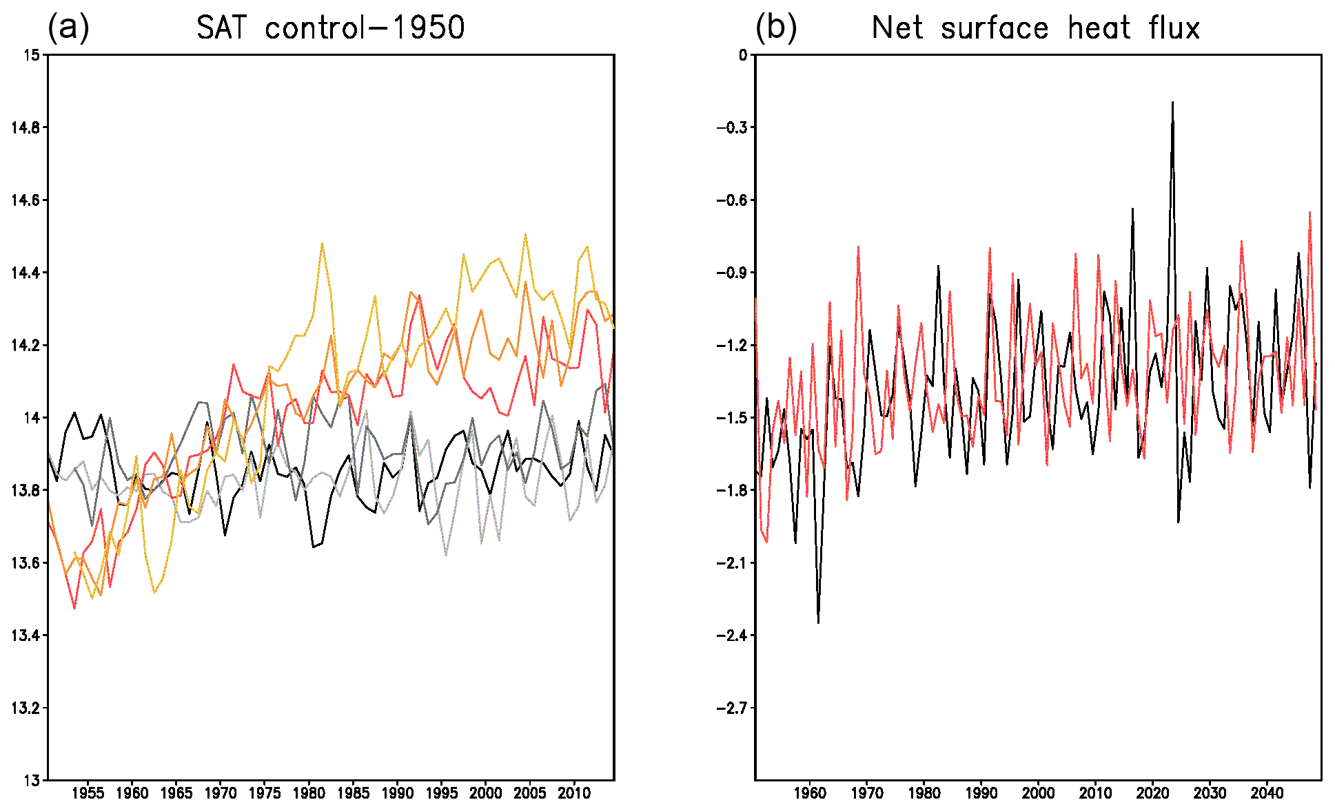
Figure 11(a) Global mean averaged annual SAT (∘C) in control-1950 for the three members of EC-Earth3P (red colors) and EC-Earth3P-HR (grey colors). (b) Global mean averaged net surface heat flux (W m−2) in control-1950 of EC-Earth3P (red) and EC-Earth3P-HR (black), displayed only for one member (r1i1p2f1) of each model for clarity; other members display similar behavior.
4.2.3 control-1950
After the spin-up, the SAT each of the three members of EC-Earth3P-HR is in quasi-equilibrium and the global mean temperature oscillates around 13.9 ∘C (Fig. 11a, black). The ocean is still warming, as expressed by a negative net surface heat flux on the order of −1.5 W m−2 (positive is upward) (Fig. 11b, black). This imbalance is reduced during the simulation but without an indication that the model is getting close to its equilibrium state.
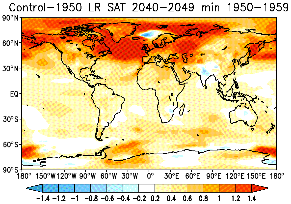
Figure 12Ensemble mean SAT (∘C) of the averaged last 10 years (2040–2049) minus the averaged first 10 years (1950–1959) of the control-1950 simulations of EC-Earth3P.
Contrary to EC-Earth3P-HR, the global annual mean SAT of EC-Earth3P displays a significant upward trend, with an indication of stabilizing after about 35 years (Fig. 11a, red). This warming trend is caused by a large warming of the North Atlantic, as revealed in Fig. 12, showing the difference between the first and last 10 years of the control-1950 run. This warming is caused by the activation of the deep convection in the Labrador Sea (not shown) that started about 10 years after the beginning of the control simulation, which was absent in the spin-up run. Associated with that, the AMOC also shows an upward trend (see Fig. 17 below). This switch to a warmer state does not strongly affect the slow warming of the deeper ocean, which is reflected in a similar behavior of the net surface heat flux to that for EC-Earth3P-HR (Fig. 11b). The reasons for the initial absence of deep convection in the Labrador Sea in EC-Earth3P and the difference with EC-Earth3P-HR are not clear and presently under investigation. Possible candidates are that the differences in ocean resolution affect the sea-ice dynamics and deep convection, but also changes in ocean temperature and salinity distribution may play a role.
The control-1950 experiment is also analyzed to evaluate model performance of internally generated variability in the coupled system; the targets are the El Niño–Southern Oscillation (ENSO), the North Atlantic Oscillation (NAO), sudden stratospheric warmings (SSWs) and the Atlantic meridional overturning circulation (AMOC).
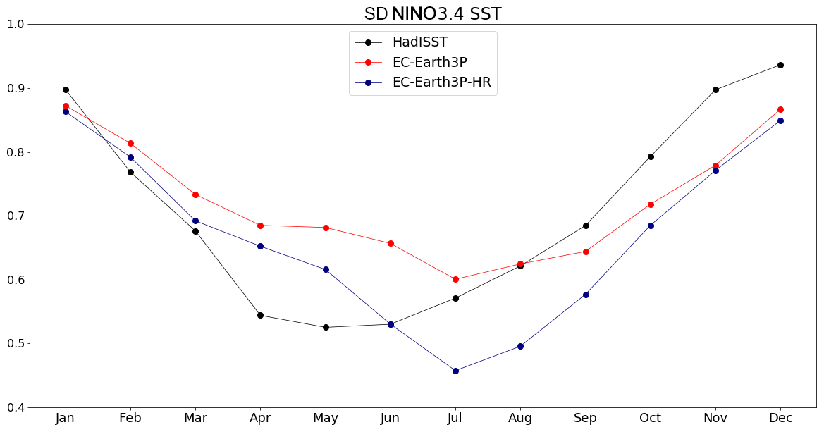
Figure 13Monthly standard deviation of the NINO3.4 SST index: EC-Earth3P (red) EC-Earth3P-HR (blue) from control-1950 and detrended Hadley Centre Sea Ice and Sea Surface Temperature data set (HadISST) over 1900–2010 (black).
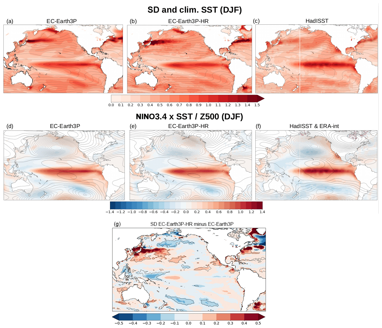
Figure 14(a–c) Boreal winter SST standard deviation from control-1950 in EC-Earth3P (a), EC-Earth3P-HR (b) and detrended HadISST (c); overplotted with contours are the corresponding climatology (contour interval 2 ∘C). Bottom: regression of SST anomalies onto the NINO3.4 index from control-1950 in EC-Earth3P (d), EC-Earth3P-HR (e) and detrended HadISST (f); overplotted with contours are the corresponding regression of 500 hPa geopotential height anomalies (c.i. 2.5 m), with ERA-Interim in panel (f). The observational period is 1979–2014. (g) Difference in SST standard deviation between EC-Earth3P-HR (b) and EC-Earth3P (a).
ENSO
Figure 13 depicts the seasonal cycle of the NINO3.4 index (SST anomalies averaged over 5∘ S–5∘ N, 170–120∘ W). As it was also shown for EC-Earth3.1 (Yang et al., 2019), both EC-Earth3P and EC-Earth3P-HR still have a systematic underestimation of the ENSO amplitude from late autumn to mid-winter and yield the minimum in July, 1–2 months later than in observations. Increasing model resolution reduces the bias in early summer (May–June) but worsens it in late summer (July–August). Overall, EC-Earth3P-HR shows lower ENSO variability than EC-Earth3P, which following Yang et al.'s (2019) arguments suggests that the ocean–atmosphere coupling strength over the tropical Pacific is weaker in the high-resolution version of the model. On the other hand, Fig. 14 displays the spatial distribution of winter SST variability and the canonical ENSO pattern, computed as linear regression onto the NINO3.4 index. Increasing model resolution leads to a reduction in the unrealistic zonal extension of the cold tongue towards the western tropical Pacific, which was also present in EC-Earth3.1 (Yang et al., 2019) and is a common bias in climate models (e.g., Guilyardi et al., 2009): EC-Earth3P reaches longitudes of Papua New Guinea (Fig. 14a), while EC-Earth3P-HR improves its location (Fig. 14b), yet overestimates it compared to observations (Fig. 14c). Note that the reduction of this model bias is statistically significant (Fig. 14g). Consistently, the improvement in the cold tongue translates into a better representation of the ENSO pattern (Fig. 14d–f). Nonetheless, the width of the cold tongue in EC-Earth3P-HR is still too narrow in the central tropical Pacific (see also Yang et al., 2019), which again is a common bias in climate models (e.g., Zhang and Jin, 2012). Both EC-Earth3P and EC-Earth3P-HR realistically simulate the wave-like structure of the ENSO teleconnection in the extratropics (Fig. 14d–f).
On another matter, note that EC-Earth3P-HR (Fig. 14b) captures the small-scale features and meanderings along the western boundary currents, Kuroshio–Oyashio and Gulf Stream, and the sea-ice edge over the Labrador Sea much better than EC-Earth3P (Fig. 14a). In these three areas, there is a substantial increase in SST variability (Fig. 14g), which following Haarsma et al. (2019) is likely due to increasing ocean resolution rather than atmosphere resolution.
NAO
Figure 15 illustrates how EC-Earth3P(-HR) simulates the surface NAO and its hemispheric signature in the middle troposphere. The NAO (here measured as leading empirical orthogonal function (EOF) of the DJF SLP anomalies over 20–90∘ N, 90∘ W–40∘ E) accounts for virtually the same fraction of SLP variance in both model versions, i.e., 42.70 % in EC-Earth3P (Fig. 15d) and 42.74 % in EC-Earth3P-HR (Fig. 15e), and still slightly underestimates the observed one (∼ 50 % in ERA-Interim, Fig. 15f); the same applied to EC-Earth2.2 when compared to ERA-40 (Hazeleger et al., 2012). EC-Earth rightly captures the circumglobal pattern associated with the NAO at upper levels (e.g., Branstator, 2002; García-Serrano and Haarsma, 2017), particularly the elongated lobe over the North Atlantic and the two centers of action over the North Pacific (Fig. 15a–c). A close inspection to the barotropic structure of the NAO reveals that the meridional dipole is shifted westward in EC-Earth3P-HR (Fig. 15b, e) as compared to EC-Earth3P (Fig. 15a, d), which according to Haarsma et al. (2019) could be related to increasing ocean resolution and a stronger forcing of the North Atlantic storm track.
SSWs
Also, the simulation of SSW occurrence is assessed (Fig. 16); the identification follows the criterion in Palmeiro et al. (2015). The decadal frequency of SSWs in EC-Earth is about eight events per decade regardless of model resolution, which is underestimated when compared to ERA-Interim (∼ 11 events per decade) but in the range of observational uncertainty (e.g., Palmeiro et al., 2015; Ayarzagüena et al., 2019). The same underestimation was diagnosed in EC-Earth3.1 (Palmeiro et al., 2020a). The reduced amount of SSWs is probably associated with a too-strong bias at the core of the polar vortex, still present in EC-Earth3.3 (Palmeiro et al., 2020b). It is thus concluded that increasing horizontal resolution does not affect the model bias in the strength of the polar vortex. The seasonal cycle of SSWs in reanalysis is quite robust over the satellite period, showing one maximum in December–January and another one in February–March (Ayarzagüena et al., 2019), which was properly captured by EC-Earth3.1 in the control, coupled simulations with fixed radiative forcing at the year 2000 (Palmeiro et al., 2020a). Here, in control-1950, EC-Earth does not reproduce such a bimodal cycle, with EC-Earth3P-HR (blue) yielding a peak in January–February and EC-Earth3P (red) two relative maxima in January and March. Interestingly, the seasonal cycle of SSWs over the historical, pre-satellite period shows a different distribution with a prominent maximum in mid-winter and a secondary peak in late winter, although it is less robust among reanalysis products (Ayarzagüena et al., 2019). The impact of the radiative forcing on SSW occurrence deserves further research.
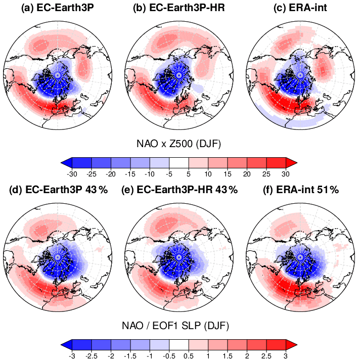
Figure 15(a–c) Regression of 500 hPa geopotential height anomalies from control-1950 in EC-Earth3P (a), EC-Earth3P-HR (b) and detrended ERA-Interim (c) onto the corresponding leading principal component, i.e., the NAO index. (d–f) Leading EOF of winter SLP anomalies over the North Atlantic–European region 20–90∘ N, 90∘ W–40∘ E, from control-1950 in EC-Earth3P (d), EC-Earth3P-HR (e) and detrended ERA-Interim (f); the corresponding fraction of explained variance is indicated in the title.
AMOC
The AMOC index was computed as the maximum stream function at 26.5∘ N and between 900 and 1200 m depth. The annual AMOC index of EC-Earth3P-HR for the control-1950 runs (Fig. 17a, black) is about 15 Sv, which is lower than the values form the RAPID array (Smeed et al., 2019) that have been measured since 2004 (stars in Fig. 17b). It reveals interannual and decadal variability, without an evident trend. As already discussed at the beginning of Sect. 4.2.3, the AMOC of EC-Earth3P shows an upward trend (Fig. 17a, red) associated with the activation of convection in the Labrador Sea.
4.2.4 hist-1950
The hist-1950 ensemble simulations differ from the control-1950 simulations in terms of the historical GHG and aerosol concentrations. The global mean annual temperature in EC-Earth3P-HR displays an increase similar to the ERA5 data set (Fig. 18a). The warming seems to be slightly larger in the model. We remind the reader, however, of the enhanced observed warming after 2014, which might result in a similar trend in the model simulations compared to observations up to present day. The cooling due to the Mt. Pinatubo eruption in 1991 is clearly visible in all members and the ensemble mean. The amplitude and period compare well with ERA5. On its part, the AMOC in EC-Earth3P-HR reveals a clear downward trend in particular from the 1990s onward (Fig. 17b, black). This is consistent with a slowdown of the Atlantic overturning due to global warming in CMIP5 models (Cheng et al., 2013).
Similarly to control-1950, the hist-1950 simulations with EC-Earth3P show an upward drift in SAT (Fig. 18a, red) and AMOC (Fig. 17b, red) that are smaller (SAT) or absent (AMOC) in EC-Earth3P-HR. The HighResMIP protocol (Haarsma et al., 2016) of having a control and a historical simulation starting from the same initial conditions was designed to minimize the consequences of such trends. Under the assumption that the model trend is similar for both simulations, it can be eliminated by subtracting the control from the historical simulation. Indeed, the global annual mean SAT and the AMOC of hist-1950 minus control-1950 display a very similar behavior in EC-Earth3P and EC-Earth3P-HR (Figs. 18b and 17c), with an upward trend for SAT and a downward trend for the AMOC. For SAT, the upward trend compares well with ERA5.

Figure 16Seasonal distribution of SSWs per decade in a [−10, 10] d window around the SSW date for ERA-Interim (black), EC-Earth3P (red) and EC-Earth3P-HR (blue) from control-1950. Time series are smoothed with an 11 d running mean. The total decadal frequency of SSWs is indicated in brackets.
Weather regimes
Another way to test the representation of the midlatitude atmospheric flow, with a focus on the low-frequency variability (5–30 d), is to assess how well the models reproduce the winter (DJF) Euro-Atlantic weather regimes (Corti et al., 1999; Dawson et al., 2012).

Figure 17Time series of the annual AMOC index for the control-1950 (a) and hist-1950 (b) runs. Solid lines display the ensemble mean for the EC-Earth3P (red) and EC-Earth3P-HR (black). Shaded areas represent the dispersion due to the ensemble members. Black stars in panel (b) display values of RAPID data. (c) Mean ensemble difference between hist-1950 and control-1950 for Earth3P (red) and EC-Earth3P-HR (black).
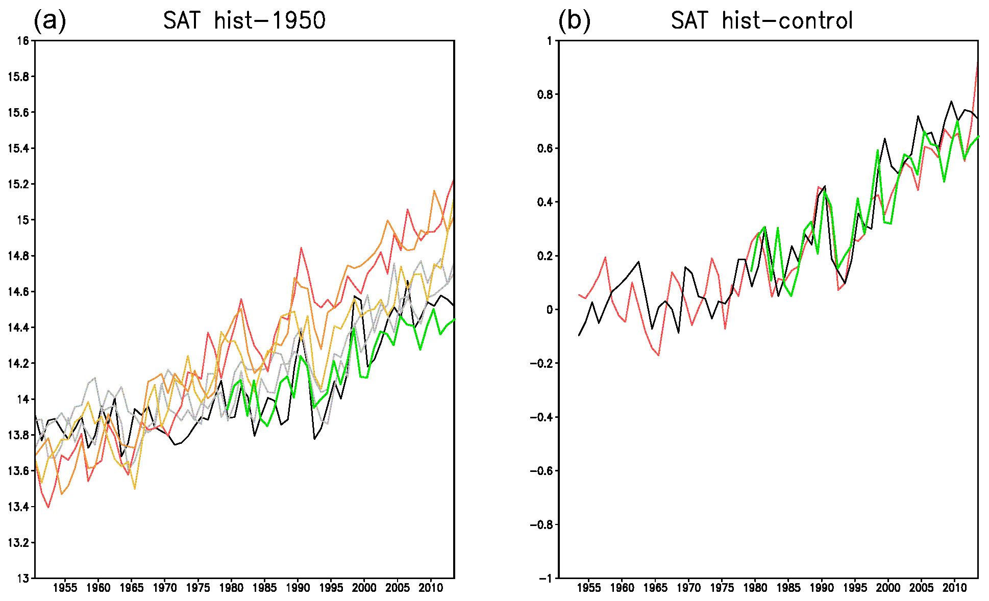
Figure 18Global mean averaged annual SAT (∘C) in hist-1950 (a) for the three members of EC-Earth3P (red colors) and EC-Earth3P-HR (grey colors). (b) Mean ensemble difference between hist-1950 and control-1950 for EC-Earth3P (red) and EC-Earth3P-HR (black). ERA5 is indicated by the green curves. Panel (b) is scaled so that the starting point fits with the EC-Earth curves.
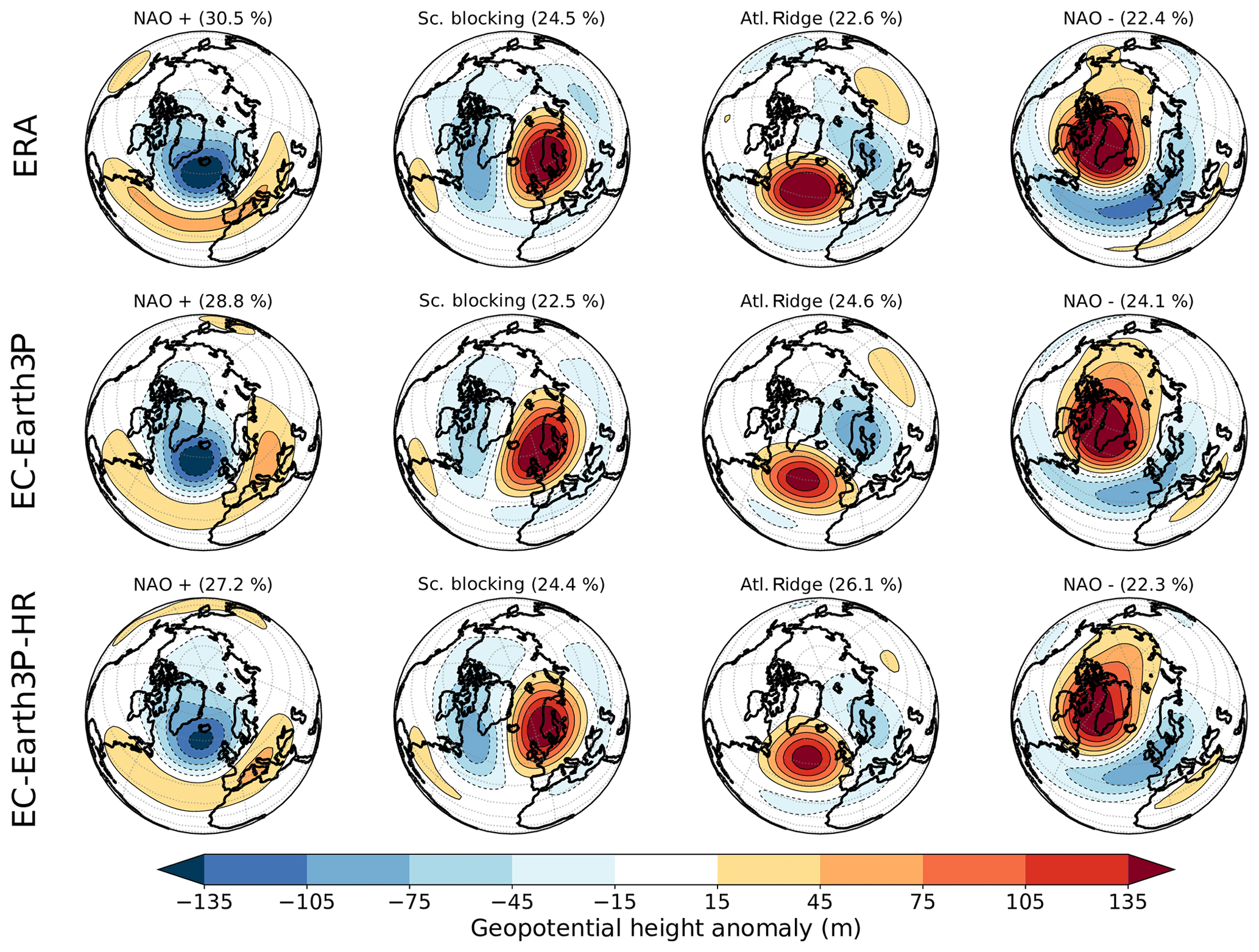
Figure 19Observed cluster patterns for ERA (a), simulated cluster patterns in hist-1950 for EC-Earth3P (b) and EC-Earth3P-HR (c). The frequency of occurrence of each regime is shown above each subplot.
The analysis has been applied here to the EC-Earth3P and EC-Earth3P-HR hist-1950 simulations. Following recent works (Dawson and Palmer, 2015; Strommen et al., 2019), we computed the regimes via k-means clustering of daily geopotential height anomalies at 500 hPa over 30–85∘ N, 80∘ W–40∘ E. As a reference, we considered the ECMWF reanalysis data from ERA40 (1957–1978) and ERA-Interim (1979–2014). The clustering is performed in the space spanned by the first four principal components obtained from the reference data set. More details on the technique used and on the metrics discussed here can be found in Fabiano et al. (2020) and references therein. Each row in Fig. 19 shows the resulting mean patterns of the four standard regimes – NAO+, Scandinavian blocking, Atlantic Ridge and NAO− – for ERA (top), EC-Earth3P (middle) and EC-Earth3P-HR (bottom). The regimes are quite well represented in both configurations. However, the matching is better in the standard-resolution version both in terms of rms and pattern correlation averaged over all regimes (see Table 3). Only the Scandinavian (Sc) blocking pattern is improved in the HR, whereas the other patterns are degraded. The most significant degradation is seen for the NAO− pattern, which is shifted westward in the HR simulation. The result for EC-Earth3P(-HR) goes in the opposite direction of what has been observed in Fabiano et al. (2020), where most models showed a tendency for improving the regime patterns with increased resolution. Concerning the regime frequencies, both model versions show a tendency to produce less NAO+ cases than the observations and more Atlantic Ridge cases (Fig. 19).
Table 3Some metrics to assess the overall performance in hist-1950 of the EC-Earth3P and EC-Earth3P-HR simulations in terms of weather regimes. The table shows the average root mean square error (RMSE) from the observed patterns and the relative average pattern correlation among all regimes, the average persistence of the two NAO states in days, the optimal ratio and the sharpness. The errors refer to the spread between members (standard deviation).
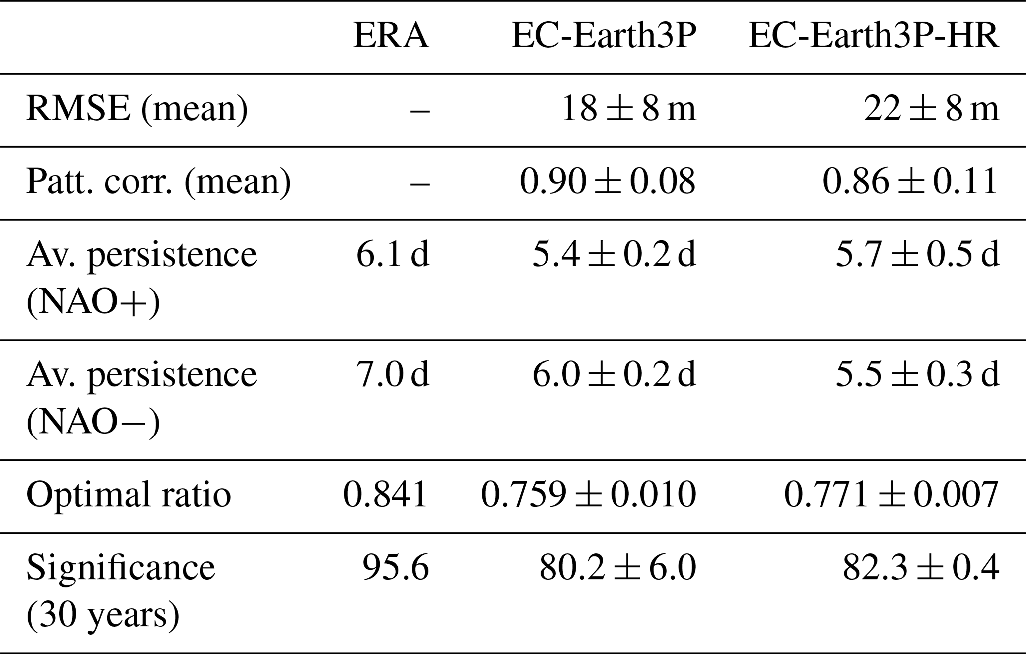
Another quantity of interest is the persistence of the regimes, since models usually are not able to reach the observed persistence of the NAO+/− states (Fabiano et al., 2020). As stated in Table 3, this is also observed for the EC-Earth3P hist-1950 simulations, and the effect of the HR is to increase the persistence of NAO+ but decrease that of NAO−.
Even if the HR is degrading the regime patterns, it produces a small but positive effect on the geometrical structure of the regimes. This is shown by the last two quantities in Table 3: the optimal ratio and the sharpness. The optimal ratio is the ratio between the mean inter-cluster squared distance and the mean intra-cluster variance: the larger the optimal ratio, the more clustered the data. The sharpness is an indicator of the statistical significance of the regime structure in the data set in comparison with a randomly sampled multi-normal distribution (Straus et al., 2007). The closer the value is to 100, the more significant the multimodality of the distribution. The sharpness tends to saturate at 100 for very long simulations, so the values reported in Table 3 are obtained from a bootstrap on 30 years chosen randomly. Both the optimal ratio and the sharpness are too low in the EC-Earth3P simulations, as is usually seen for all models. A significant increase with EC-Earth3P-HR is seen for the optimal ratio, and a smaller (non-significant) one is seen for the sharpness.
The increased resolution simulations have a stronger regime structure and are closer to the observations in this sense. However, the regime patterns are degraded in the HR version and this affects the resulting atmospheric flow. A similar result was obtained by Strommen et al. (2019) for a different version of EC-Earth and two other climate models.
As contribution of the EC-Earth consortium to HighResMIP, a new version of EC-Earth has been developed with two horizontal resolutions: the standard-resolution EC-Earth3P (T255, ORCA1) and the high-resolution EC-Earth3P-HR (T511, ORCA0.25). Simulations following the HighResMIP protocol (Haarsma et al., 2016) for all three tiers have been made using both resolutions, with an ensemble size of three members. Only the spin-up consists of one member.
Performing 100-year simulations for the high-resolution version (EC-Earth3P-HR) required specific developments for the hardware and software to ensure efficient production, post-processing and storage of the data. In addition, the model must be able to run on different platforms with similar performance. Large efforts have been dedicated to scalability, reducing bottlenecks during performance, computational optimization and efficient post-processing and data output.
Enhancing resolution does not noticeably affect most model biases and there are even locations and variables where increasing the resolution has a deteriorating effect such as an increase of the wet bias over the warm pool seen in the highresSST-present simulations or the representation of Euro-Atlantic weather regimes found in the hist-1950 experiments. Also, the variability reveals examples of improvement such as the zonal extension of the ENSO pattern or the representation of meandering along the western boundary currents, as revealed in the control-1950 simulations. The lack of re-tuning the high-resolution version of the model compared to the standard-resolution version, in accordance with the HighResMIP protocol, might be responsible for this.
The short spin-up as prescribed by the HighResMIP protocol prevented the simulations from reaching an equilibrium state. This happened in particular for the control-1950 and hist-1950 simulations of EC-Earth3P, where a transition to a warmer state occurred due to enhanced convection in the Labrador Sea, with an accompanying increase of the AMOC. Because this transition occurred almost concurrently in the control-1950 and hist-1950 simulations, the greenhouse-forced warming from 1950 onward in EC-Earth3P can be inferred by subtracting both simulations. The resulting warming pattern compares well with the observed one and is similar to the warming pattern simulated by EC-Earth3P-HR. Due to the transition, the control-1950 does not provide a near-equilibrium state. It was therefore decided to extend the control-1950 run for another 100 years to allow process studies that will be documented elsewhere.
Analysis of the kinetic energy spectrum indicates that the subsynoptic scales are better resolved at higher resolution (Klaver et al., 2020) in EC-Earth. Despite the lack of a clear improvement with respect to biases and synoptic-scale variability for the high-resolution version of EC-Earth, the better representation of subsynoptic scales results in better representation of phenomena and processes on these scales such as tropical cyclones (Roberts et al., 2020) and ocean–atmosphere interaction along western boundary currents (Tsartsali et al., 2020).
Model codes developed at ECMWF, including the IFS and FVM, are intellectual property of ECMWF and its member states. Permission to access the EC-Earth source code can be requested from the EC-Earth community via the EC-Earth website (http://www.ec-earth.org/, last access: July 2020) and may be granted if a corresponding software license agreement is signed with ECMWF. The repo tags for the versions of IFS and EC-Earth that are used in this work are 3.0p (see Sect. 4.2, “p1” version) and 3.1p (“p2” version), and are available through r7481 and r7482 on ECSF, respectively. The model code evaluated in the paper has been provided for anonymous review by the topical editor and anonymous reviewers.
The DOIs of the data used in the analyses and available from ESGF are as follows:
-
EC-Earth3P: https://doi.org/10.22033/ESGF/CMIP6.2322 (EC-Earth, 2019),
-
EC-Earth3P-HR: https://doi.org/10.22033/ESGF/CMIP6.2323 (EC-Earth, 2018).
RH, MA, PAB, LPC, MC, SC, PD, FB, JG-G, TK, VM, TvN, FMP, MR, PLS, MvW and KW contributed to the text and the analyses. All authors contributed to the design of the experiment, model development, simulations and post-processing of the data.
The authors declare that they have no conflict of interest.
The EC-Earth simulations from SMHI were performed on resources provided by the Swedish National Infrastructure for Computing (SNIC). The EC-EARTH simulations from BSC were performed on resources provided by ECMWF and the Partnership for Advanced Computing in Europe (PRACE; MareNostrum, Spain).
Froila M. Palmeiro and Javier García-Serrano were partially supported by the Spanish GRAVITOCAST project (ERC2018-092835) and the “Ramón y Cajal” program (RYC-2016-21181), respectively, and MR was supported by “Beca de collaboració amb la Universitat de Barcelona” (2019.4.FFIS.1).
The EC-Earth simulations from CNR were performed on resources provided by CINECA and ECMWF (special projects SPITDAVI and SPITMAVI).
The EC-Earth simulations from KNMI were partly performed on resources provided by ECMWF (special project SPNLHAAR).
This research has been supported by the European Commission (grant nos. PRIMAVERA (641727), SPFireSD (748750), INADEC (800154), and STARS (754433)).
This paper was edited by Paul Ullrich and reviewed by two anonymous referees.
Acosta, M. C., Yepes-Arbós, X., Valcke, S., Maisonnave, E., Serradell, K. , Mula-Valls, O., and Doblas-Reyes, F. J.: Performance analysis of EC-Earth 3.2: Coupling, BSC-CES Technical Memorandum 2016-006, 38 pp., 2016.
Adler, R. F., Huffman, G. J., Chang, A., Ferraro, R., Xie, P. P., Janowiak, J., Rudolf, B., Schneider, U., Curtis, S., Bolvin, D., Gruber, A., Susskind, J., Arkin, P., and Nelkin, E.: The version-2 global precipitation climatology project (gpcp) monthly precipitation analysis (1979–present), J. Hydrometeorol., 4, 1147–1167, 2003.
Ayarzagüena, B., Palmeiro, F. M., Barriopedro, D., Calvo, N., Langematz, U., and Shibata, K.: On the representation of major stratospheric warmings in reanalyses, Atmos. Chem. Phys., 19, 9469–9484, https://doi.org/10.5194/acp-19-9469-2019, 2019.
Balsamo, G., Beljaars, A., Scipal, K., Viterbo, P., van den Hurk,B., Hirschi, M., and Betts, A. K.: A revised hydrology for theECMWF model: Verification from field site to terrestrial waterstorage and impact in the Integrated Forecast System, J. Hydrometeorol., 10, 623–643, 2009.
Batté, L. and Doblas-Reyes, F. J.: Stochastic atmospheric perturbations in the EC-Earth3 global coupled model: Impact of SPPT on seasonal forecast quality, Clim. Dynam., 45, 3419–3439, 2015.
Bellprat, O., Massonnet, F., García-Serrano, J., Fučkar, N. S., Guemas, V., and Doblas-Reyes, F. J.: The role of Arctic sea ice and sea surface temperatures on the cold 2015 February over North America, in: Explaining Extreme Events of 2015 from a Climate Perspective, B. Am. Meteorol. Soc., 97, S36–S41, https://doi.org/10.1175/BAMS-D-16-0159.1, 2016.
Branstator, G.: Circumglobal teleconnections, the jet stream waveguide, and the North Atlantic Oscillation, J. Climate, 15, 1893–1910, 2002.
Brodeau, L. and Koenigk, T.: Extinction of the northern oceanic deep convection in an ensemble of climate model simulations of the 20th and 21st centuries, Clim. Dynam., 46, 2863–2882, 2016.
Caron, L.-P., Jones, C. J., and Doblas-Reyes, F. J.: Multi-year prediction skill of Atlantic hurricane activity in CMIP5 decadal hindcasts, Clim. Dynam., 42, 2675–2690, https://doi.org/10.1007/s00382-013-1773-1, 2014.
Corti, S., Molteni, F., and Palmer, T.: Signature of recent climate change in frequencies of natural atmospheric circulation regimes, Nature, 398, 799–802, https://doi.org/10.1038/19745, 1999.
Cheng, W., Chiang, J. C., and Zhang, D.: Atlantic meridional overturning circulation (AMOC) in CMIP5 models: RCP and historical simulations, J. Climate, 26, 7187–7197, 2013.
Craig, A., Valcke, S., and Coquart, L.: Development and performance of a new version of the OASIS coupler, OASIS3-MCT_3.0, Geosci. Model Dev., 10, 3297–3308, https://doi.org/10.5194/gmd-10-3297-2017, 2017.
Davini, P., von Hardenberg, J., and Corti, S.: Tropical origin for the impacts of the Atlantic Multidecadal Variability on the Euro-Atlantic climate, Environ. Res. Lett., 10, 094010, https://doi.org/10.1088/1748-9326/10/9/094010, 2015.
Dawson, A., and Palmer, T. N.: Simulating weather regimes: Impact of model resolution and stochastic parameterization, Clim. Dynam., 44, 2177–2193, 2015.
Dawson, A., Palmer, T. N., and Corti, S.: Simulating regime structures in weather and climate prediction models, Geophys. Res. Lett., 39, L21805, https://doi.org/10.1029/2012GL053284, 2012.
Dee, D. P., Uppala, S. M., Simmons, A. J., Berrisford, P., Poli, P., Kobayashi, S., Andrae, U., Balmaseda, M. A., Balsamo, G., Bauer, P., Bechtold, P., Beljaars, A. C. M., van de Berg, I., Biblot, J., Bormann, N., Delsol, C., Dragani, R., Fuentes, M., Greer, A. J., Haimberger, L., Healy, S. B., Hersbach, H., Holm, E. V., Isaksen, L., Kallberg, P., Kohler, M., Matricardi, M., McNally, A. P., Mong-Sanz, B. M., Morcette, J.-J., Park, B.-K., Peubey, C., de Rosnay, P., Tavolato, C., Thepaut, J. N., and Vitart, F.: The ERA-Interim reanalysis: Configuration and performance of the data assimilation system, Q. J. Roy. Meteorol. Soc., 137, 553–597, https://doi.org/10.1002/qj.828, 2011.
Doblas-Reyes, F. J., Andreu-Burillo, I., Chikamoto, Y., García-Serrano, J., Guemas, V., Kimoto, M., Mochizuki, T., Rodrigues L. R. L., and van Oldenborgh, G. J.: Initialized near-term regional climate change prediction, Nat. Commun., 4, 1–9, 2013.
Doescher, et al.: The EC-Earth3 Earth System Model for the Climate Model Intercomparison Project 6, Geosci. Model Dev., submitted, 2020.
EC-Earth Consortium (EC-Earth): EC-Earth-Consortium EC-Earth3P-HR model output prepared for CMIP6 HighResMIP, https://doi.org/10.22033/ESGF/CMIP6.2323, 2018.
EC-Earth Consortium (EC-Earth): EC-Earth-Consortium EC-Earth3P model output prepared for CMIP6 HighResMIP, https://doi.org/10.22033/ESGF/CMIP6.2322, 2019.
Eyring, V., Bony, S., Meehl, G. A., Senior, C. A., Stevens, B., Stouffer, R. J., and Taylor, K. E.: Overview of the Coupled Model Intercomparison Project Phase 6 (CMIP6) experimental design and organization, Geosci. Model Dev., 9, 1937–1958, https://doi.org/10.5194/gmd-9-1937-2016, 2016.
Fabiano, F., Christensen, H. M., Strommen, K., Athanasiadis, P., Baker, A., Schiemann, R., and Corti, S.: Euro-Atlantic weather Regimes in the PRIMAVERA coupled climate simulations: impact of resolution and mean state biases on model performance, Clim. Dynam., 5031–5048, https://doi.org/10.1007/s00382-020-05271-w, 2020.
García-Serrano, J. and Haarsma, R. J.: Non-annular, hemispheric signature of the winter North Atlantic Oscillation, Clim. Dynam., 48, 3659–3670, 2017.
Guemas, V., Doblas-Reyes, F. J., Andreu-Burillo, I., and Asif, M.: Retrospective prediction of the global warming slowdown in the past decade, Nat. Clim. Change, 3, 649–653, https://doi.org/10.1038/nclimate1863, 2013.
Guemas, V., García-Serrano, J., Mariotti, A., Doblas-Reyes, F. J., and Caron, L.-P.: Prospects for decadal climate prediction in the Mediterranean region, Q. J. Roy. Meteor. Soc., 687, 580–597, https://doi.org/10.1002/qj.2379, 2015.
Good, S. A., Martin, M. J., and Rayner, N. A.: EN4: Quality controlled ocean temperature and salinity profiles and monthly objective analyses with uncertainty estimates, J. Geophys. Res., 118, 6704–6716, https://doi.org/10.1002/2013JC009067, 2013.
Guilyardi, E., Wittenberg, A., Fedorov, A., Collins, M., Wang, C., Capotondi, A., van Oldenborgh, G. J., and Stockdale, T.: Understanding El Niño in ocean-atmosphere general circulation models, B. Am. Meteorol. Soc., 90, 325–340, 2009.
Haarsma, R. J., Roberts, M. J., Vidale, P. L., Senior, C. A., Bellucci, A., Bao, Q., Chang, P., Corti, S., Fučkar, N. S., Guemas, V., von Hardenberg, J., Hazeleger, W., Kodama, C., Koenigk, T., Leung, L. R., Lu, J., Luo, J.-J., Mao, J., Mizielinski, M. S., Mizuta, R., Nobre, P., Satoh, M., Scoccimarro, E., Semmler, T., Small, J., and von Storch, J.-S.: High Resolution Model Intercomparison Project (HighResMIP v1.0) for CMIP6, Geosci. Model Dev., 9, 4185–4208, https://doi.org/10.5194/gmd-9-4185-2016, 2016.
Haarsma, R. J., García-Serrano, J., Prodhomme, C., Bellprat, O., Davini, P., and Drijfhout, S.: Sensitivity of winter North Atlantic-European climate to resolved atmosphere and ocean dynamics, Sci. Rep., 9, 13358, https://doi.org/10.1038/s41598-019-49865-9, 2019.
Hazeleger, W., Severijns, C., Semmler, T., Ştefănescu, S., Yang, S., Wang, X., Wyser, K., Dutra, E., Baldasano, J. M., Bintanja, R., Bougeault, P., Caballero, R., Ekman, A. M. L., Christensen, J. H., van den Hurk, B., Jimenez, P., Jones, C., Kållberg, P., Koenigk, T., McGrath, R., Miranda, P., van Noije, T., Palmer, T., Parodi, J. A., Schmith, T., Selten, F., Storelvmo, T., Sterl, A., Tapamo, H., Vancoppenolle, M., Viterbo, P., and Willén, U.: EC-Earth: a seamless earth-system prediction approach in action, B. Am. Meteorol. Soc., 91, 1357–1364, 2010.
Hazeleger, W., Wang, X., Severijns, C., Ştefănescu, S., Bintanja, R., Sterl, A., Wyser, K., Semmler, T., Yang, S., van den Hurk, B., van Noije, T., van der Linden, E., and van der Wiel, K.: EC-Earth V2.2: description and validation of a new seamless earth system prediction model, Clim. Dynam., 39, 2611–2629, 2012.
Hersbach, H., Bell, B., Berrisford, P., Hirahara, S., Horányi, A., Muñoz-Sabater, J., Nicolas,J., Peubey, C., Radu, R., Schepers, D., Simmons, A., Soci, C., Abdalla, S., Abellan, X., Balsamo, G., Bechtold, P., Biavati, G., Bidlot, J., Bonavita, M., De Chiara, G., Dahlgren, P., Dee, D., Diamantakis, M., Dragani, R., Flemming, J., Forbes, R., Fuentes, M., Geer, A., Haimberger, L., Healy, S., Hogan, R. J., Hólm, E., Janisková, M., Keeley, S., Laloyaux, P., Lopez, P., Lupu, C., Radnoti, G., de Rosnay, P., Rozum, I., Vamborg, F., Villaume, S., and Thépaut, J.-N.: The ERA5 global reanalysis, Q. J. Roy. Meteor. Soc., 1–51, https://doi.org/10.1002/qj.3803, 2020.
IPCC: Climate Change 2013: The Physical Science Basis, in: Contribution of Working Group I to the Fifth Assessment Report of the Intergovernmental Panel on Climate Change, edited by: Stocker, T. F., Qin, D., Plattner, G.-K., Tignor, M., Allen, S. K., Boschung, J., Nauels, A., Xia, Y., Bex, V., and Midgley, P. M., Cambridge University Press, Cambridge, UK, New York, NY, USA, 1535 pp., https://doi.org/10.1017/CBO9781107415324, 2013.
Kennedy, J., Titchner, H., Rayner, N., and Roberts, M.: Input4mips.MOHC.sstsandseaice.highresmip.MOHC-hadisst-2-2-0-0-0, Earth System Grid Federation, https://doi.org/10.22033/ESGF/input4mips.1221, 2017.
Klaver, R., Haarsma, R., Vidale, P. L., and Hazeleger, W.: Effective resolution in high resolution global atmospheric models for climate studies, Atmos. Sci. Lett., 21, e952, https://doi.org/10.1002/asl.952, 2020.
Koenigk, T. and Brodeau, L.: Ocean heat transport into the Arctic in the twentieth and twenty-first century in EC-Earth, Clim. Dynam., 42, 3101–3120, 2014.
Koenigk, T. and Brodeau, L.: Arctic climate and its interaction with lower latitudes under different levels of anthropogenic warming in a global coupled climate model, Clim. Dynam., 49, 471–492, 2017.
Koenigk, T., Brodeau, L., Graversen, R. G., Karlsson, J., Svensson, G., Tjernström, M., Willén, U., and Wyser, K.: Arctic climate change in 21st century CMIP5 simulations with EC-Earth, Clim. Dynam., 40, 2719–2743, 2013.
Madec, G.: NEMO reference manual, ocean dynamic component: NEMO-OPA, Note du Pôle modélisation, Inst. Pierre Simon Laplace, France, 2008.
Madec, G. and the NEMO team: NEMO ocean engine version 3.6 stable, Note du Pôle de modélisation de l'Institut Pierre-Simon Laplace No. 27, ISSN: 1288-1619, 2016.
Myriokefalitakis, S., Daskalakis, N., Gkouvousis, A., Hilboll, A., van Noije, T., Williams, J. E., Le Sager, P., Huijnen, V., Houweling, S., Bergman, T., Nüß, J. R., Vrekoussis, M., Kanakidou, M., and Krol, M. C.: Description and evaluation of a detailed gas-phase chemistry scheme in the TM5-MP global chemistry transport model (r112), Geosci. Model Dev. Discuss., https://doi.org/10.5194/gmd-2020-110, in review, 2020.
Palmeiro, F. M., Barriopedro, D., García-Herrera, R., and Calvo, N.: Comparing sudden stratospheric warming definitions in reanalysis data, J. Climate, 28, 6823–6840, 2015.
Palmeiro, F. M., García-Serrano, J., Bellprat, O., Bretonnière, P. A., and Doblas-Reyes, F. J.: Boreal winter stratospheric variability in EC-EARTH: high-top vs. low-top, Clim. Dynam., 54, 3135–3150, 2020a.
Palmeiro, F. M., García-Serrano, J., Ábalo, M., and Christiansen, B.: Boreal winter stratospheric climatology in EC-EARTH, Clim. Dynam., in preparation, 2020b.
Poli, P., Hersbach, H., Dee, D. P., Berrisford, P., Simmons, A. J., Vitart, F., Laloyaux, P., Tan, D. G. H., Peubey, C., Thépaut, J.-N., Trémolet, Y., Hólm; E. V., Bonavita, M., Isaksen, L., and Fisher, M.: ERA-20C: An atmospheric reanalysis of the twentieth century, J. Climate, 29, 4083–4097, 2016.
Prodhomme, C., Batté, L., Massonnet, F., Davini, P., Bellprat, O., Guemas, V., and Doblas-Reyes, F. J.: Benefits of increasing the model resolution for the seasonal forecast quality in EC-Earth, J. Climate, 29, 9141–9162, 2016.
Roberts, M. J., Vidale, P. L., Senior, C., Hewitt, H. T., Bates, C., Berthou, S., Chang, P., Christensen, H. M., Danilov, S., Demory, M.-E., Griffies, S. M., Haarsma, R., Jung, T., Martin, G., Minobe, S., Ringler, T., Satoh, M., Schiemann, R., Scoccimarro, E., Stephens, G., and Wehner, M. F.: The Benefits of Global High Resolution for Climate Simulation: Process Understanding and the Enabling of Stakeholder Decisions at the Regional Scale, B. Am. Meteorol. Soc., 99, 2341–2359, 2018.
Roberts, M., Camp, J., Seddon, J., Vidale, P. L., Hodges, K., Vanniere. B., Mecking, J., Haarsma, R., Bellucci, A., Scoccimarro, E., Caron, L.-P., Chauvin, F., Terray, L., Valcke, S., Moine, M.-P., Putrasahan, D., Roberts., C., Senan, R., Zarzycki, C., and Ullrich, P.: Impact of model resolution on tropical cyclone simulation using the HighResMIP-PRIMAVERA multi-model ensemble, J. Climate, 33, 2557–2583, 2020.
Rodgers, K. B., Aumont, O., Mikaloff Fletcher, S. E., Plancherel, Y., Bopp, L., de Boyer Montégut, C., Iudicone, D., Keeling, R. F., Madec, G., and Wanninkhof, R.: Strong sensitivity of Southern Ocean carbon uptake and nutrient cycling to wind stirring, Biogeosciences, 11, 4077–4098, https://doi.org/10.5194/bg-11-4077-2014, 2014.
Smeed, D., Moat, B., Rayner, D., Johns, W. E., Baringer, M. O., Volkov, D., and Frajka-Williams E.: Atlantic meridional overturning circulation observed by the RAPID-MOCHA-WBTS (RAPID-Meridional Overturning Circulation and Heatflux Array-Western Boundary Time Series) array at 26∘ N from 2004 to 2018, British Oceanographic Data Centre – Natural Environment Research Council, UK, https://doi.org/10.5285/8cd7e7bb-9a20-05d8-e053-6c86abc012c2, 2019.
Solaraju Murali, B., Caron, L.-P., González-Reviriego, N., and Doblas-Reyes, F. J.: Multi-year prediction of European summer drought conditions for the agricultural sector. Environ. Res. Lett., 14, 124014 https://doi.org/10.1088/1748-9326/ab5043., 2019.
Sterl, A., Bintanja, R., Brodeau, L., Gleeson, E., Koenigk, T., Schmith, T., Semmler, T., Severijns, C., Wyser, K., and Yang, S.: A look at the ocean in the EC-Earth climate model, Clim. Dynam., 39, 2631–2657, 2012.
Straus, D. M., Corti, S., and Molteni, F.: Circulation regimes: Chaotic variability versus SST forced predictability, J. Climate, 20, 2251–2272, 2007.
Strommen, K., Mavilia, I., Corti, S., Matsueda, M., Davini, P., von Hardenberg, J., Vidale, P.-L., and Mizuta, R.: The Sensitivity of Euro-Atlantic Regimes to Model Horizontal Resolution, Geophys. Res. Lett., 46, 7810–7818, 2019.
Tintó, O., Acosta, M., Castrillo, M., Cortés, A., Sanchez, A., Serradell, K., and Doblas-Reyes, F. J.: Optimizing domain decomposition in an ocean model: the case of NEMO, Procedia Comput. Sci., 108, 776–785, 2017.
Tintó Prims O., Castrillo, M., Acosta, M.C., Mula-Valls, O., Sanchez Lorente, A., Serradell, K., Cortés A., and Doblas-Reyes F. J.: Finding, analysing and solving MPI communication bottlenecks in Earth System models, J. Comput. Sci., 36, 100864, https://doi.org/10.1016/j.jocs.2018.04.015, 2019.
Tsartsali, E., Haarsma, R., de Vries, H., Bellucci, A., Athanasiadis, P., Scoccimarro, E., Ruggieri, P., Gualdi, S., Fedele, G., Garcia-Serrano, J., Castrillo, M., Putrahasan, D., Sanchez-Gomez, E., Moine, M.-P., Roberts, C. D., Roberts, M. J., Seddon, J., and Vidale, P. L.: Impact of resolution on atmosphere-ocean VMM and PAM coupling along the Gulf stream in global high resolution models, in preparation, 2020.
Valcke, S. and Morel, T.: OASIS and PALM, the CERFACS couplers, Tech. rep., CERFACS, 2006.
Vancoppenolle, M., Bouillon, S., Fichefet, T., Goosse, H., Lecomte, O., Morales Maqueda, M. A., and Madec, G.: The Louvain-la-Neuve sea ice model, Notes du pole de modélisation, Institut Pierre-Simon Laplace (IPSL), Paris, France, No. 31, 2012.
van Noije, T. P. C., Le Sager, P., Segers, A. J., van Velthoven, P. F. J., Krol, M. C., Hazeleger, W., Williams, A. G., and Chambers, S. D.: Simulation of tropospheric chemistry and aerosols with the climate model EC-Earth, Geosci. Model Dev., 7, 2435–2475, https://doi.org/10.5194/gmd-7-2435-2014, 2014.
Yang, C., Christensen, H. M., Corti, S., von Hardenberg, J., and Davini, P.: The impact of stochastic physics on the El Niño Southern Oscillation in the EC-Earth coupled model, Clim. Dynam., 53, 2843–2859, 2019.
Zhang, W. and Jin, F.-F.: Improvements in the CMIP5 simulations of the ENSO-SSTA meridional width, Geophys. Res. Lett., 39, L23704, https://doi.org/10.1029/2012GL053588, 2012.