the Creative Commons Attribution 4.0 License.
the Creative Commons Attribution 4.0 License.
 | 05 Aug 2020
Concentration Trajectory Route of Air pollution with an Integrated Lagrangian model (C-TRAIL Model v1.0) derived from the Community Multiscale Air Quality Model (CMAQ Model v5.2)
Arman Pouyaei
Jia Jung
Bavand Sadeghi
Chul Han Song
This paper introduces a novel Lagrangian model (Concentration Trajectory Route of Air pollution with an Integrated Lagrangian model, C-TRAIL version 1.0) output from a Eulerian air quality model for validating the source–receptor direct link by following polluted air masses. To investigate the concentrations and trajectories of air masses simultaneously, we implement the trajectory-grid (TG) Lagrangian advection scheme in the CMAQ (Community Multiscale Air Quality) Eulerian model version 5.2. The TG algorithm follows the concentrations of representative air “packets” of species along trajectories determined by the wind field. The diagnostic output from C-TRAIL accurately identifies the origins of pollutants. For validation, we analyze the results of C-TRAIL during the KORUS-AQ campaign over South Korea. Initially, we implement C-TRAIL in a simulation of CO concentrations with an emphasis on the long- and short-range transport effects. The output from C-TRAIL reveals that local trajectories were responsible for CO concentrations over Seoul during the stagnant period (17–22 May 2016) and during the extreme pollution period (25–28 May 2016), highly polluted air masses from China were distinguished as sources of CO transported to the Seoul Metropolitan Area (SMA). We conclude that during the study period, long-range transport played a crucial role in high CO concentrations over the receptor area. Furthermore, for May 2016, we find that the potential sources of CO over the SMA were the result of either local transport or long-range transport from the Shandong Peninsula and, in some cases, from regions north of the SMA. By identifying the trajectories of CO concentrations, one can use the results from C-TRAIL to directly link strong potential sources of pollutants to a receptor in specific regions during various time frames.
- Article
(11831 KB) - Full-text XML
-
Supplement
(982 KB) - BibTeX
- EndNote


Determining the long-range transport (LRT) of pollutants has been a challenge for air quality researchers. As the chemical composition of outflow over a region or continent can significantly affect air quality downwind, information about LRT must be reliable. Several studies have applied a number of methods to examine the role that LRT plays in the concentrations of particulate matter (PM), ozone, trace gases, and biomass burning tracers over target regions (Stohl, 2002). For instance, in an attempt to identify possible sources of PM in East Asia, several studies (Choi et al., 2014; Lee et al., 2019; Oh et al., 2015; Pu et al., 2015) have applied the NOAA Hybrid Single-Particle Lagrangian Integrated Trajectory (HYSPLIT) model (Draxler, 1998) and back-trajectory analysis. A number of researchers have incorporated the widely used HYSPLIT model into other chemical-transport models (CTMs) to measure the LRT of ozone, carbon monoxide (CO), and aerosols to establish the source–receptor relationship of air masses over the United States (Bertschi and Jaffe, 2005; Carroll et al., 2008; Gratz et al., 2015; Price et al., 2004; Sadeghi et al., 2020; Weiss-Penzias et al., 2004). Several studies have used another model, the FLEXTRA trajectory model (Stohl, 1996; Stohl and Seibert, 1998), to capture the background source regions of high PM over East Asia and quantify the contributions from these regions (Lee et al., 2011, 2013). Furthermore, this model has also been applied to some European regions to explain the potential advected contribution of aerosols (Cristofanelli et al., 2007; Petetin et al., 2014; Salvador et al., 2008). Several studies have recently attempted to develop new trajectory models that overcome truncation errors that originate from schemes for numerically integrating trajectory equations (Döös et al., 2017; Rößler et al., 2018) and to link trajectories to specific trace species (Kruse et al., 2018; Stenke et al., 2009). Another widely used tool for studying the distribution of CO, ozone, PM, and other aerosols for both air quality forecasting and emission scenario analysis is the EPA Community Multiscale Air Quality (CMAQ) model (Byun and Schere, 2006). CMAQ, supported by meteorological inputs from the Weather Research and Forecasting (WRF) model – or advanced machine learning-based methods (Eslami et al., 2019; Lops et al., 2019; Sayeed et al., 2020) – assists policy-makers with solving pollution-related issues by legislating regulations. Spatial concentration patterns of pollutants incorporated with other models (i.e., back-trajectory models) or satellite data enhance our understanding of the impact of LRT and other related processes such as the formation of aerosols, emissions, and dry deposition in various regions (Chen et al., 2014; Chuang et al., 2008, 2018; Souri et al., 2016; Wang et al., 2010; Xu et al., 2019; Zhang et al., 2019).
The conventional way of estimating potential source regions of air-mass transport is to use back-trajectory modeling. Frequently used for source–receptor linkage, such models combine their output with measurements of pollutant concentrations. As this source–receptor linkage approach uses meteorology-based models for back trajectories, it is not fully accepted because it is unable to directly determine whether an originated air mass is polluted or non-polluted (Lee et al., 2019). Thus, back-trajectory modeling sometimes provides unreliable information from which to assess the variation in pollutants at a receptor point, raising concern about its use for interpreting the contribution of the effect of LRT on concentrations of a target pollutant. In addition, other factors such as emissions and the local production of air pollutants contribute to variation in a target pollutant. Although aircraft campaigns in several regions have applied a Lagrangian approach for interpreting variations in concentrations, they have not effectively addressed the above concern. After all, such campaigns are neither frequent nor continuous.
In this study, we implement a Lagrangian advection scheme that we refer to as the trajectory grid (TG) (Chock et al., 1996) into the Eulerian CMAQ v5.2 model. We introduce a new type of output from the Concentration Trajectory Route of Air pollution with the Integrated Lagrangian (C-TRAIL v1.0) stand-alone model in addition to CMAQ v5.2 output to simultaneously accomplish two objectives: (1) to provide a direct link between polluted air masses from sources and a receptor and (2) to provide the spatial concentration distribution of several pollutants that explains relevant physical processes. Chock et al. (2005) incorporated the TG into an air quality model to study the accuracy of this Lagrangian advection method over the Bott advection scheme applied in the Eulerian domain. One significant outcome of the TG model applied to CTMs is its ability to account for the concentrations of pollutants in air masses in its investigation of trajectories. This outcome addresses the unreliability of meteorology-based Lagrangian models when the pollutedness or cleanliness of an originated air mass becomes an issue. For this study, we have selected CO as our trace gas target. As this pollutant has an oxidation lifetime of approximately 2 months, it is an ideal tracer with which we can study its impact on LRT without having stable background levels such as CO2 (Heald et al., 2003; Liu et al., 2010; Vay et al., 2011). Furthermore, as CO is produced mainly by the incomplete combustion of carbon-containing fuels (Halliday et al., 2019), it is an ideal proxy with which we can relate concentrations of receptors to sources of traffic or power-plant emissions. We begin by introducing the methodology behind TG and the implementation of TG into CMAQ. Then, we present a simple case and our interpretation of the C-TRAIL output. Finally, we present a case study of C-TRAIL for Korea and the United States Air Quality (KORUS-AQ) campaign over South Korea.
2.1 Description of the TG approach
To solve the transport equation, Chock et al. (1996) presented the TG approach in air quality modeling. This approach, which entails transporting points on a concentration profile along their trajectories in a Lagrangian manner, uses the Eulerian approach for diffusive transport. From now on, we will refer to these points as “air packets” for two reasons: (1) their nature is similar to that of air parcels, but they are massless, and (2) they behave much like particles, but they carry information about several species. The TG method rewrites the advection equation for concentration as follows:
where C is the concentration of species in velocity field v. The Lagrangian approach divides the total derivative of the concentration into a full derivative of concentration with respect to time, , and a remaining term containing velocity divergence, . Following this approach, the TG automatically and accurately conserves the mass, sign, and shape of the concentration profile. As interpreted from the equation, the concentration profile of the species along trajectories can be described. Otherwise stated, after determining the location of a packet and the concentration inside the domain, we are able to assess the concentration profile along its trajectory. Since all species represented in one packet and all of the packets move in the flow field according to the wind velocity, differentiating among advection equations for each species (as is done in Eulerian advection schemes) is no longer necessary; thus, this approach removes the associated numerical errors with the discretization of the advection equation. The concentration of each packet along its trajectory can be determined by the following equation:
where C(t) is the concentration of species at the location of a packet as it moves along its trajectory. Since we can use the TG method to calculate the concentration from an ordinary differential equation, it is mass conserving, monotonic, and accurate. Although interpolation errors occur during the diffusion step, they are typically considerably smaller than Eulerian advection errors (Chock et al., 2005). In addition, the trajectory will be three-dimensional and as accurate as the input for wind velocity and direction. In particular, for large-scale vertical winds, in which CTMs typically modify the scheme to address the mass-conservation issue, TG removes numerical diffusion from upwind vertical advection schemes and generates more physical vertical winds (Hu and Talat Odman, 2008). It is worth mentioning that units for the concentration of species are referred to as parts per billion by volume (ppbv) or micrograms per cubic meter (µg m−3) , depending on the species type, and the unit conversion is taken into account in the process of solving equations.
2.2 Implementation of TG in CMAQ v5.2
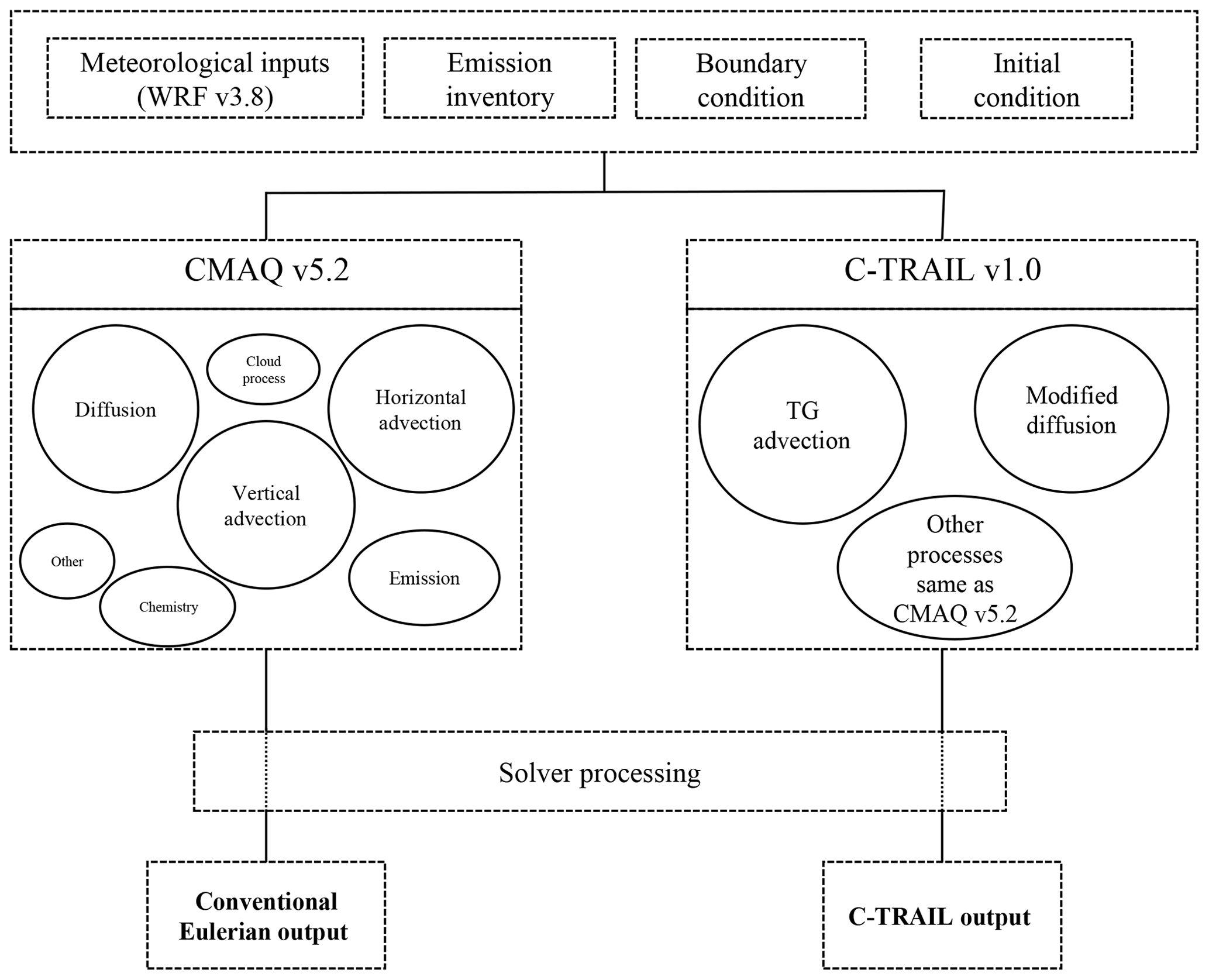
In this section, we briefly describe the key features of TG implementation in the CMAQ v5.2 model, a Eulerian model consisting of several modules (i.e., advection, diffusion, cloud, and aqueous-phase). The C-TRAIL v1.0 model requires the same meteorology, initial conditions (ICs), boundary conditions (BCs), and emissions as CMAQ. All CMAQ modules and parameters are associated with cells of the Eulerian grid in the model domain. Since TG is based on CMAQ in this study and some of the CMAQ processes cannot be satisfactorily carried out by Lagrangian models (e.g., eddy diffusion) at this time, grid cells are the primary structure for initiating and listing packets. By grouping the packets into grid cells, keeping track of which packets are close to each other is easier. While the grid cells of Eulerian models represent Eulerian-type outputs, tracking the packets of Lagrangian advection provides both their trajectories and their concentrations (Fig. 1).
The process of advection for packets follows the ordinary differential equation:
where V) is the three-dimensional wind velocity, and y(t) (m) is the position vector of packets at time t (s). The equation is solved using the following simple predictor-corrector scheme:
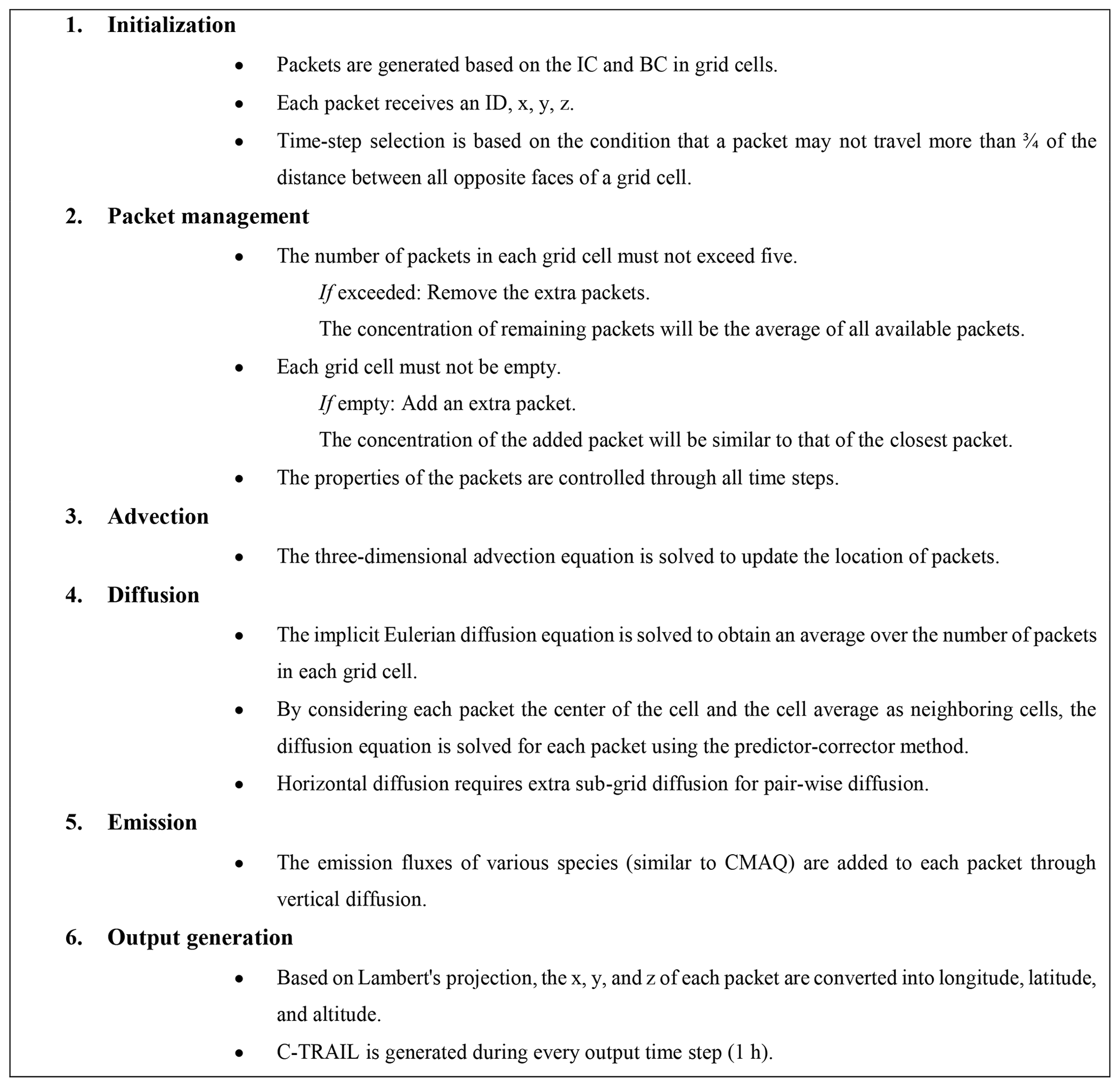
where yi is the initial estimate of the new position from the predictor step, and yf is the final position calculated by the corrector step. When the initiated packets in the domain follow the Lagrangian equation, they land in different grid cells after each time step. To balance the density of packets in grid cells, we apply a simple packet management technique that includes spawning (filling) and pruning (emptying) processes. In the spawning process, every step entails the creation of a group of new packets in each cell with insufficient packets. The initial composition of a spawned packet is estimated from nearby packets. The pruning process entails the removal of extra packets from cells that have become overpopulated. During this process, the packets closest to the cell center are retained. Such packet management with favorable options contributes to reducing the computational costs of the C-TRAIL model. The limitation of this packet management approach, however, is that it violates mass conservation. These errors are caused by sub-grid interpolations of packets in the spawning or pruning process. The underlying algorithms for both vertical and horizontal diffusion, emissions, and other processes are the same as those in standard CMAQ (Byun and Schere, 2006) with some minor modifications. The coupling of Eulerian diffusion and TG advection at each time step is accomplished by first taking the average of concentrations from all packets in each cell as the cell average. Then, by considering each packet as a cell and cell average representative of neighboring cells, we use a predictor-corrector method to determine the concentration of each packet. In addition, the C-TRAIL model considers convective transport only for resolved clouds (when clouds cover an entire grid). The WRF model implements the cloud model to obtain cloud properties on a sub-grid scale and addresses vertical transport on a resolved scale (Kain, 2004). Outputs from the WRF model are used in the CMAQ's cloud model to account for convective transport in two separate modules: sub-grid-scale clouds and resolved clouds (Byun and Schere, 2006). In this version of C-TRAIL for convection, we only use vertical winds determined from resolved clouds (see Table S1 in the Supplement). Figure 2 summarizes the process of C-TRAIL from initialization to output generation. By combining the locations of the packets from each time step during the 24 h, we generate the 24 h trajectory of each packet.
In this study, we implement TG in the CMAQ model version 5.2. Shown in Fig. 3, the model domain, with a horizontal grid resolution of 27 km over East Asia, covers the eastern parts of China, the Korean Peninsula, and Japan. We use the 2010 MIX emission inventory (Li et al., 2017) at a 0.25∘ spatial resolution. The emission inventory contains monthly averaged carbon bond version 5 (Sarwar et al., 2012) emission information, which includes 10 chemical species, including CO, in five different sectors. We also use the 2011 Clean Air Policy Support System emission high-resolution (1 km) inventory from the National Institute of Environmental Research for Korea, which contains the area and the line and point sources of a variety of species, including CO. We provide WRF model v3.8 output as the meteorological input in our CMAQ model. We validate the wind predictions from our WRF model with surface measurements and radiosonde measurements from the KORUS-AQ period (see Tables S2–S3 and Figs. S1–S4 in the Supplement). Jung et al. (2019) validated the air quality model setup by comparing simulated and observed aerosol optical depths; the research showed a correlation of 0.64 for the entire KORUS-AQ campaign period. Its comparison of various gaseous and particulate species also showed close agreement with observations.
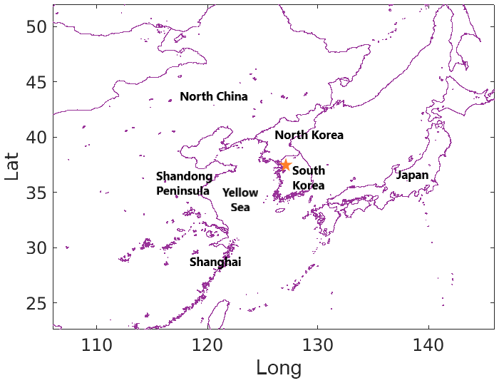
Figure 3Domain of the study; the orange star indicates the Seoul Metropolitan Area (SMA).
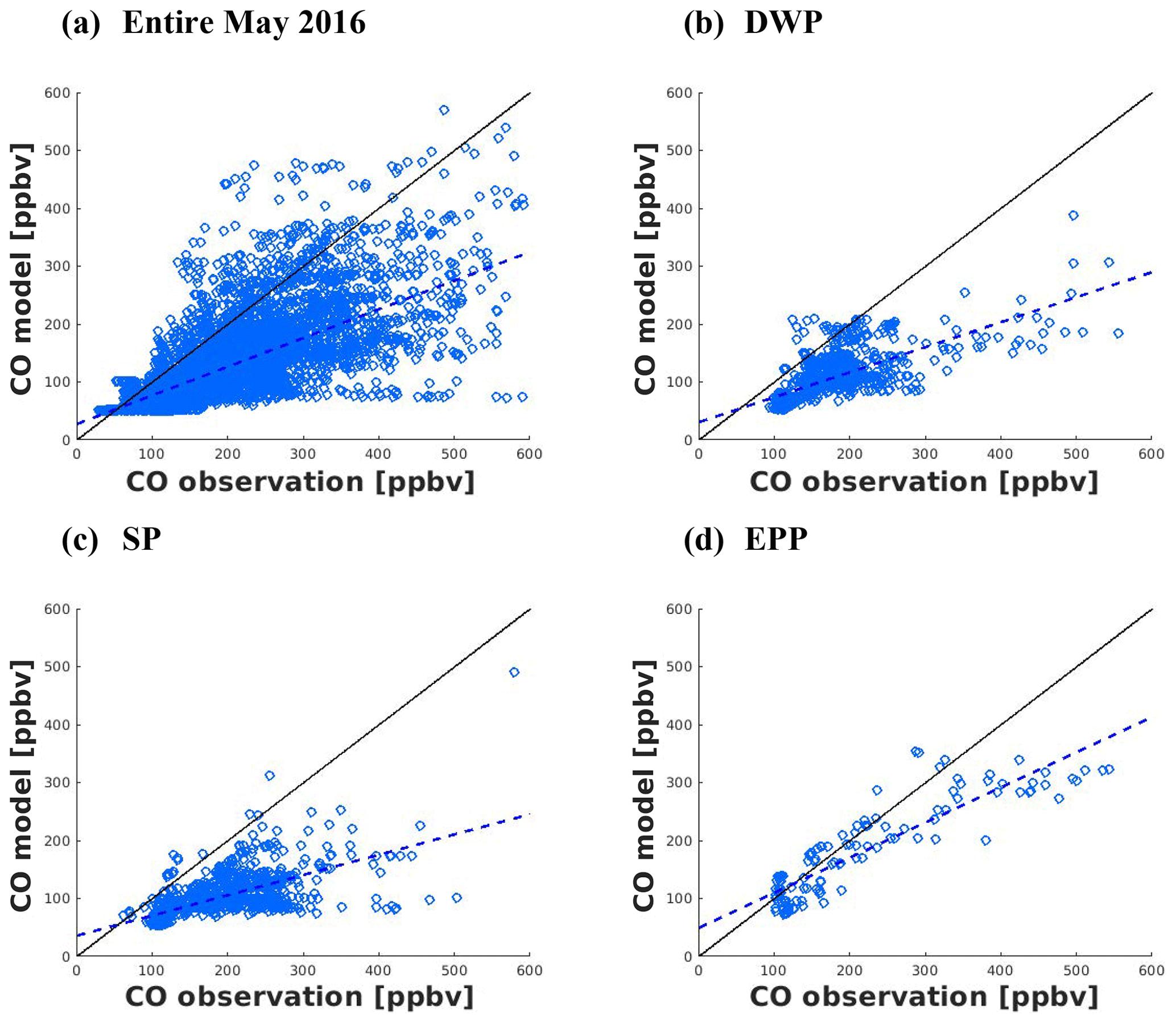
Figure 4CMAQ model results versus aircraft CO measurements for (a) the entire month of May 2016 (n=6865), (b) the DWP (n=1750), (c) the SP (n=1548), and (d) the EPP (n=264).
We run C-TRAIL simulations for May 2016 during the KORUS-AQ campaign. Studies pertaining to this campaign (Al-Saadi et al., 2016; Choi et al., 2019; Miyazaki et al., 2019) have separated the time frame into three periods (Table 1) based on meteorological conditions: (1) the dynamic weather period (DWP), a rapid cycle of clear and rainy days in the Korean Peninsula (10–16 May); (2) the stagnant period (SP), in which the area was under the influence of a high-pressure system (17–22 May) and which showed the influence of local emissions; and (3) the extreme pollution period (EPP) with high peaks of pollutants that showed strong direct transport from China (25–28 May).
Table 1Comparison of the statistical parameters of CMAQ CO concentrations to aircraft measurements (COR: correlation; IOA: index of agreement; RMSE: root mean square error; MAE: mean absolute error).
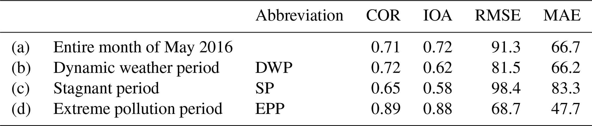
The overall accuracy of the CMAQ CO simulation compared to aircraft measurements during all periods is presented in Fig. 4a. The correlation between the modeled CO concentrations and observations at various altitudes for the entire month of May 2016 was 0.71, indicating that the performance of the model is sufficiently reliable for a study of the sources of CO concentration (Table 1). Figure 4 illustrates the underprediction of the model during the DWP and SP. However, the model shows a high correlation during the EPP compared to higher CO observations over the Korean Peninsula. We also provide a CMAQ CO comparison with surface station measurements in the Supplement (see Table S4 and Fig. S5). The results of this comparison also show the underprediction of the model, caused by uncertain emission inventories over East Asia. The C-TRAIL outputs of the mentioned periods will be discussed in Sect. 3.3.

Figure 5Model CO concentrations and wind patterns over the surface during (a) the entire month of May 2016, (b) the DWP, (c) the SP, and (d) the EPP.
The Eulerian output from CMAQ, including CO concentrations and surface wind fields, is displayed in Fig. 5. High peaks of CO concentrations appeared in southeastern China, including the Shanghai region and the Shandong Peninsula, because of high anthropogenic emissions in these areas. The impact on pollution from LRT was greater in this region because the dominant wind over East Asia in May was westerly, which explains our observations of high CO concentrations over the Yellow Sea. We also observed a shallow anticyclone (a common phenomenon that affects the regional transport of pollution in this region) over the Yellow Sea during the study period. From a thorough investigation of CO concentrations and wind patterns during various meteorological periods, we present the following major findings. (1) During the DWP, a mixed response from the LRT of CO and local emissions occurred. Also, considering the impact of convection, the concentrations of CO over Korea could have been increased or decreased because of vertical wind transport and cloud updrafts and downdrafts. Owing to the dynamic nature of this period (i.e., cloudy, rainy, or clear), the interpretation of the LRT effect by conventional methods poses a challenge. (2) During the SP, a high-pressure system settled over the Korean Peninsula, which explains the extremely low wind speed and the stagnant air, the latter of which eliminated the impact of LRT. Even though one might assume that the model would produce more accurate simulations with less convection-related transport, CO concentrations were significantly underestimated by the model (Jeon et al., 2016) because of uncertainties in the chemistry modeling and the faulty emission inventories over East Asia. (3) During EPP, as shown in Fig. 5, the anticyclone over the Yellow Sea contributed to the transport of more CO from China to the Korean Peninsula. We also observed high concentrations of CO in regions throughout ChinaṪhus, the combination of these two effects produced model predictions of higher concentrations over Korea.
The raw hypothesis from Eulerian outputs is that a high CO concentration at a receptor during a specific period is due to LRT from a source because the direction of the wind is typically toward the receptor during the period of simulation. This hypothesis is based on the average wind speed and direction and the average CO concentration, which do not constitute a reliable source of this assumption. We will briefly explain why we require merged output with simultaneous changes in trajectories and concentrations. To determine the source of LRT, researchers should include one major parameter in their investigations: the trajectory of the air mass. Once the location of the source and the trajectory of the air mass are known, the air mass is assumed to be polluted. If the air mass is not polluted, then that source is not responsible for high concentrations in the receptor location. Therefore, linking the source to the receptor based on only mean wind patterns and concentrations is not a reliable approach. The following section will discuss how we combine concentrations and trajectories into one set of outputs to explain the trajectories more clearly.
Because C-TRAIL is a diagnostic tool derived from CMAQ, both a Lagrangian output and CMAQ standard Eulerian output are available after each run. C-TRAIL helps us identify the source–receptor linkage, save the full trajectory of packets, and display the path of selected packets. Therefore, C-TRAIL simulations not only provide all spatial concentration changes but also display the trajectories of each packet, owing to the Lagrangian approach of TG. In addition, we are able to determine changes in concentrations along this trajectory. The difference between this model and other meteorological-based models is that they enable us to study changes in the concentrations of selected species along different paths, investigate evidence for the amount of pollution in originated air masses, study the reason behind the oscillation of concentrations, and examine the linkage of oscillations to both sources and sinks along the path.
This section provides an example of how we use C-TRAIL to study the sources of different packets from different altitudes (from below 1 to almost 10 km) over the Seoul Metropolitan Area (SMA); later sections will focus on the entire month of May 2016 C-TRAIL over the SMA and provide more comprehensive illustrations of the concentrations and altitudes of trajectories. Figure 6 displays the C-TRAIL output for 4 June 2016. We gathered all of the packets over the city of Seoul and analyzed the trajectory of each packet. Figure 6a shows the path of all the packets, represented by various colors, from their sources. We observed that some of the packets came from southeastern South Korea, and one originated in southeastern China, traveled over the Yellow Sea, and landed in Seoul. Some of the packets also originated from northwest of South Korea and northern China. Most of the packets, however, were locally initiated, generally from regions around the SMA. Using the HYSPLIT back-trajectory model, we found relatively similar trajectories (Fig. S6).
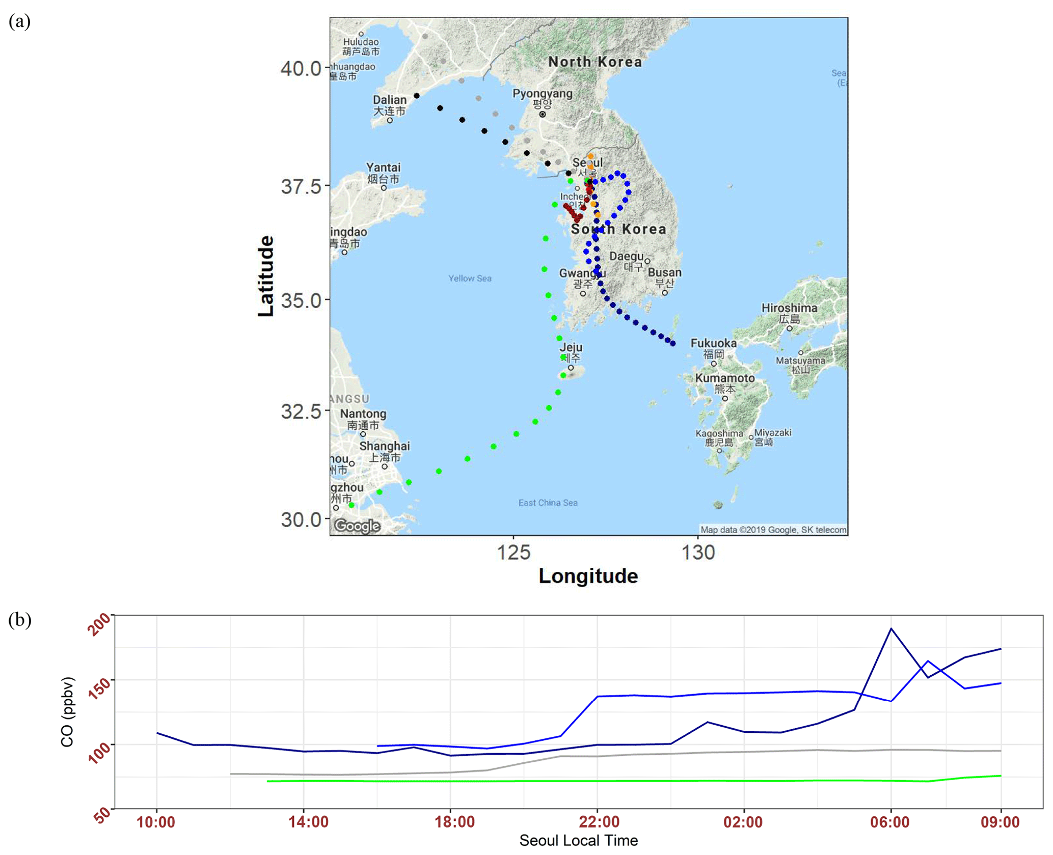
Figure 6C-TRAIL output for 4 June 2016: (a) the trajectory of packets reaching Seoul at 09:00 local time (b) changes in the CO concentrations of four aged packets moving toward Seoul from source points.
Figure 6b depicts how the CO concentrations of the four most aged packets changed as they traveled on their path toward Seoul. This type of output is a new feature that has not been studied before. With meteorological-based back-trajectory models, the path of air parcels and their back trajectories can be delineated; we are the first, however, to use a CMAQ-based Lagrangian integrated model to study the concentrations of species (in this case, CO) via the paths of air packets. The four most aged packets came from 24, 21, 20, and 17 time steps back (Fig. 6b). We find these packets interesting because they follow a long path, changes in their concentrations fluctuate, and they are easy to comprehend. From studying these packets and their C-TRAILs, we generally understand that the concentration of each packet increases as it approaches the SMA. The concentrations of near-surface packets tend to fluctuate more than those of high-altitude packets (Fig. S7). Also, larger oscillations in the concentrations occur over land rather than over the ocean, which, however, becomes more vivid when a near-surface packet reaches land from the ocean and suddenly peaks in concentration. The sudden peaks in the concentrations of near-surface packets are due to their movement over either a city or some source of emissions. Over the SMA and other cities, two peaks, mainly caused by on-road traffic emissions, occur during local morning and evening times.
Using a conventional method with model data gathered over the course of a month or a year to incorporate concentrations into a trajectory analysis produces a tremendous amount of outputs that are difficult to interpret simultaneously. For our case study, covering May 2016, we selected Seoul, South Korea, over East Asia as the receptor. We plotted C-TRAIL outputs according to variations in the packet concentrations and their distances from the receptor. Figure 7a presents the general path of all packet trajectories reaching the Seoul area at various altitudes at 09:00 local time throughout May 2016. The color bar represents the altitude at which the packets were traveling. Generally, packets at low altitudes traveled from local areas to Seoul, and those at high altitudes traveled from more distant regions. One exception was packets that originated in the Shandong Peninsula; Some traveled at high altitudes and some at low altitudes. Figure 7b displays a C-TRAIL that represented a unique type of packet that followed the concentrations of trajectories. In this case, each packet at each location (or hour of the trajectory) had a specific CO concentration that depended on its altitude (high altitude/surface), its location (land/sea/urban/forest), and the hour of the day (traffic hours/non-traffic hours). To more clearly explain the location of packets and the variability in their trajectory paths before reaching Seoul, we created a boxplot of packet distances in kilometers from the receptor at each hour before the packets reached Seoul, shown in Fig. 7c. When the packets reached Seoul at 09:00 local time, the distance became zero. Furthermore, boxplots of trajectory heights for all periods is presented in Fig. S8. In a study of C-TRAIL outputs, it is better to account for trajectories, concentrations, and distances simultaneously. As a result, the concentrations and distances of packets in early hours (10:00 to 14:00 local time) in Fig. 7 show high variability in concentrations with a median of around 150 ppbv and a maximum as high as 500 ppbv. Most of these packets originated far from the receptor (i.e., eastern, northern, and southeastern China). The median concentration, shown in boxplots, rose slightly between 18:00 and 22:00 local time. Distances also showed more variation during this time, which could be explained by the different paths of the trajectories (i.e., local trajectories with shorter distances and LRT trajectories with longer distances). As the packets approached Seoul (06:00 to 09:00 local time), the upper whisker of concentration values increased to as high as 400 ppbv, and the distances approached zero, indicating higher concentrations of CO of local trajectories resulting from surface on-road emissions and other emission sources.
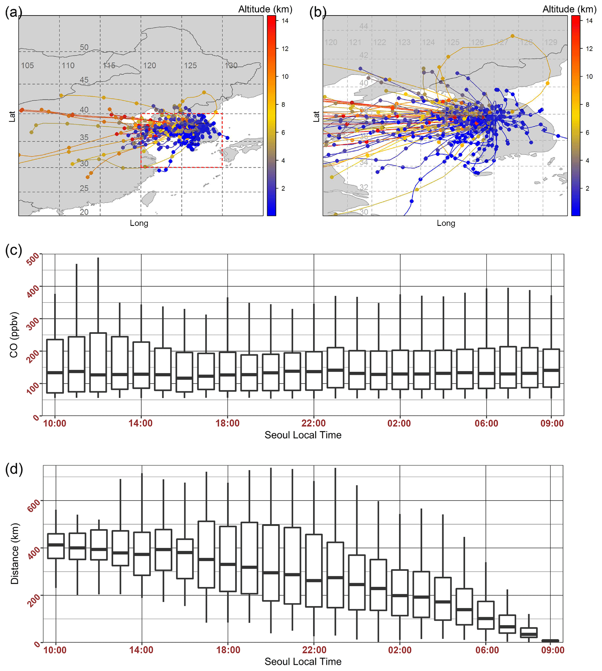
Figure 7C-TRAIL output for the entire month of May 2016 for Seoul as the receptor: (a) 24 h trajectories of packets for the entire domain, (b) 24 h trajectories of packets for the zoomed area in South Korea, (c) boxplots of the CO concentrations of all packets at each hour before they reached Seoul, and (d) boxplots of packet distances from Seoul at each hour before the packets reached Seoul.
Because of variable weather and wind (i.e., cloudy, rainy, or clear) during the DWP, C-TRAIL showed a mixed response of trajectories from both local and long-range transport, shown in Fig. 8a. A wide interquartile range and a median of close to the 25th percentile at 11:00 and 12:00 local time indicate that a few packets contained high concentrations of CO (close to 300 ppbv), but the majority consisted of low concentrations (around 100 ppbv). The distance output of low-concentration packets showed distances as long as 500 km (over the Shandong Peninsula). As the packets approached Seoul, the median concentration values were as high as 150 ppbv. Thus, from Fig. 8, we conclude that most of the long trajectories followed a path at high altitudes (higher than 7 km), and the polluted trajectories, which originated in the Shandong Peninsula, were from the near surface, shown in Fig. 8a.
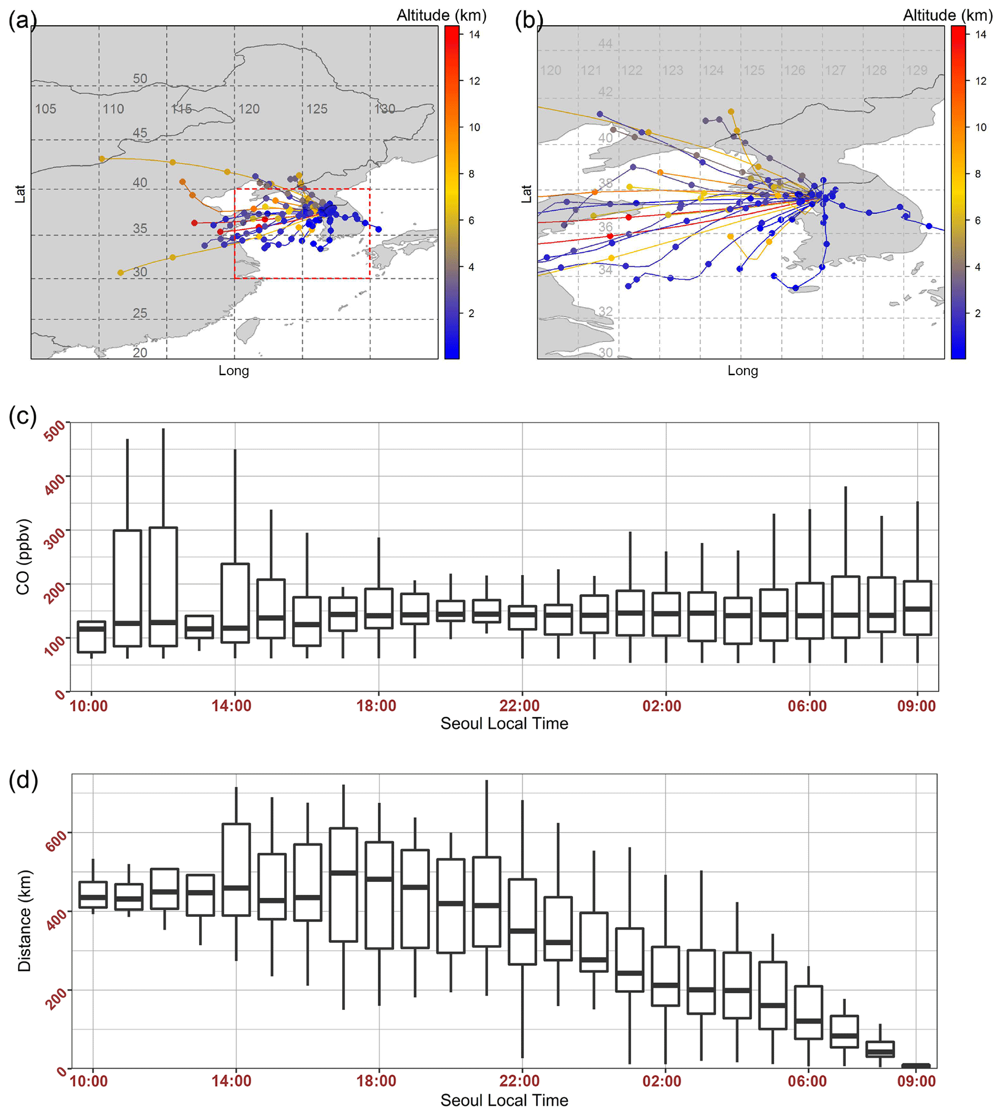
Figure 8C-TRAIL output for the dynamic weather period (DWP) for Seoul as the receptor: (a) 24 h trajectories of packets for the entire domain, (b) 24 h trajectories of packets for the zoomed area in South Korea, (c) boxplots of the CO concentrations of all packets at each hour before they reached Seoul, and (d) boxplots of packet distances from Seoul at each hour before the packets reached Seoul.
Unlike the DWP, the SP showed a more vivid display of trajectories, nearly all of which could be considered local trajectories. Long-range trajectories could not be considered responsible for the CO concentration values of Seoul. After all, from 10:00 to 16:00 local time (Fig. 9a and b), nearly all of the long-distance packets had concentrations of less than 100 ppbv. The local origination of highly polluted trajectories can be explained by a high-pressure system over the Korean Peninsula during this time period, which was responsible for very low wind speeds. The poor emission inventory over East Asia, however, provided extreme underpredictions of high concentration values during this time period. Therefore, when studying model outputs, we should account for various aspects of the model (e.g., the transport, diffusion, formation, deposition, and convention), in which diffusion, in this case, played a significant role in CO concentration values at the receptor location.

Figure 9C-TRAIL output for the stagnant period (SP) for Seoul as the receptor: (a) 24 h trajectories of packets for the entire domain, (b) 24 h trajectories of packets for the zoomed area in South Korea, (c) boxplots of the CO concentrations of all packets at each hour before they reached Seoul, and (d) boxplots of packet distances from Seoul at each hour before the packets reached Seoul.
During the EPP, several high concentrations of CO appeared at the early points of trajectories. These high concentrations, combined with high distance values, indicate that the LRT of polluted air masses was responsible for high concentrations of CO during this time period (Fig. 10). Furthermore, the variability in CO concentrations from 22:00 to 09:00 local time at the receptor location stemmed from both the various paths of the trajectories and the distances. High concentration trajectories close to the surface, which originated in the Shandong Peninsula, passed over the Yellow Sea and landed in Seoul at 09:00 local time. When the surface packets reached urban areas, they presented maximum CO concentrations, depending on the time of day and the rush-hour traffic. An assumption made by studies that used Eulerian model outputs or meteorological-based Lagrangian models for this time period was that transport played an important role (Lee et al., 2019). The outputs from C-TRAIL also indicate that highly polluted air masses originated in China (the source) and landed in Seoul (the receptor). That is, the findings of this study regarding the trajectories and the origin of polluted air masses are similar to those of previous studies.

Figure 10C-TRAIL output for the extreme pollution period (EPP) for Seoul as the receptor: (a) 24 h trajectories of packets for the entire domain, (b) 24 h trajectories of packets for the zoomed area in South Korea, (c) boxplots of the CO concentrations of all packets at each hour before they reached Seoul, and (d) boxplots of packet distances from Seoul at each hour before the packets reached Seoul.
We further analyzed the diverse aspects of C-TRAIL results using the openair package in R (Carslaw and Ropkins, 2012) and determined the frequency of trajectories passing through every gridded area, illustrated in Fig. 11a. Central China, northern China, and North Korea were not common areas for packet movement because the packets most likely passed only once through the grids of these regions (at a frequency of about 1%). For the Yellow Sea and the Shandong Peninsula region, however, trajectories more likely passed at a frequency of about 10 %. The figure also shows that most of the trajectories (25 % to 100 %) passed over the west side of the SMA, a area (the dark-red section in Fig. 11a). We can classify trajectories into separate segments according to their concentrations. Figure 11b shows this type of classification and the link between the average concentration of all trajectories to their paths. While higher concentrations were most likely the result of local transport, lower concentrations were most likely from LRT. For the May 2016 case, while most of the high concentration values corresponded to packets that originated in South Korea or close to the SMA, most of the low concentration values corresponded to packets originating in China. Their impact, however, is still evident.
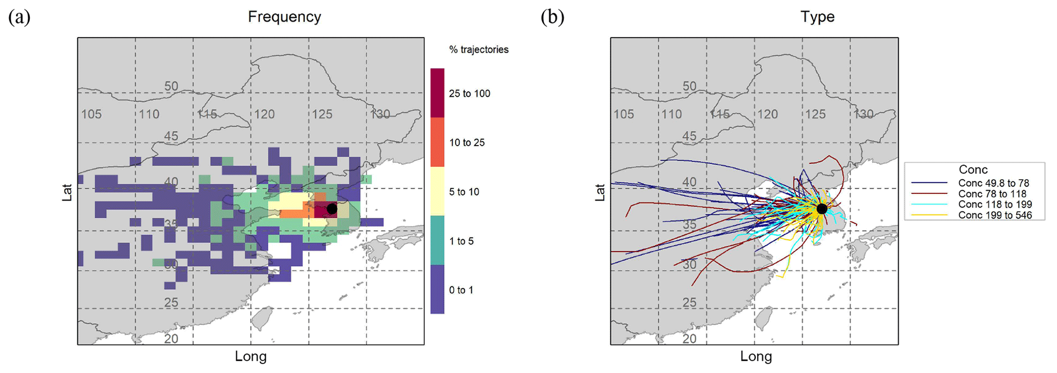
Figure 11(a) Plot of the frequency of trajectories and (b) the trajectories, classified by their concentration values.
By clustering the outputs of C-TRAIL, we are better able to locate the dominant paths for the May 2016 trajectories. According to Fig. 12a, based on the Euclidean distance function, about 37.8 % of trajectories originated in local areas east, south, and north of the SMA. About 16.1 % of trajectories originated in northern China and followed paths over the Yellow Sea to the SMA; about 10.5 % of the trajectories came from southwestern South Korea and traveled over the Yellow Sea to reach the SMA; about 21.3 % of trajectories came from the Shandong Peninsula, and the remaining trajectories (5.3 %) originated in central China and were transported over China and the Yellow Sea to the SMA. Angle clustering in Fig. 12b, however, tells a different story about the trajectories. Clustering by the angle distance function shows a similarity among the angles from the starting points of the back trajectories. Generally, nearly all of the packets originated from west of the SMA, with 32.2 % farther west, 34.5 % southwest, 12.7 % south-southwest, and 14.9 % northwest; only 5.7 % originated from east-southeast of the SMA. This clustering is consistent with strong westerly winds during the spring in East Asia.
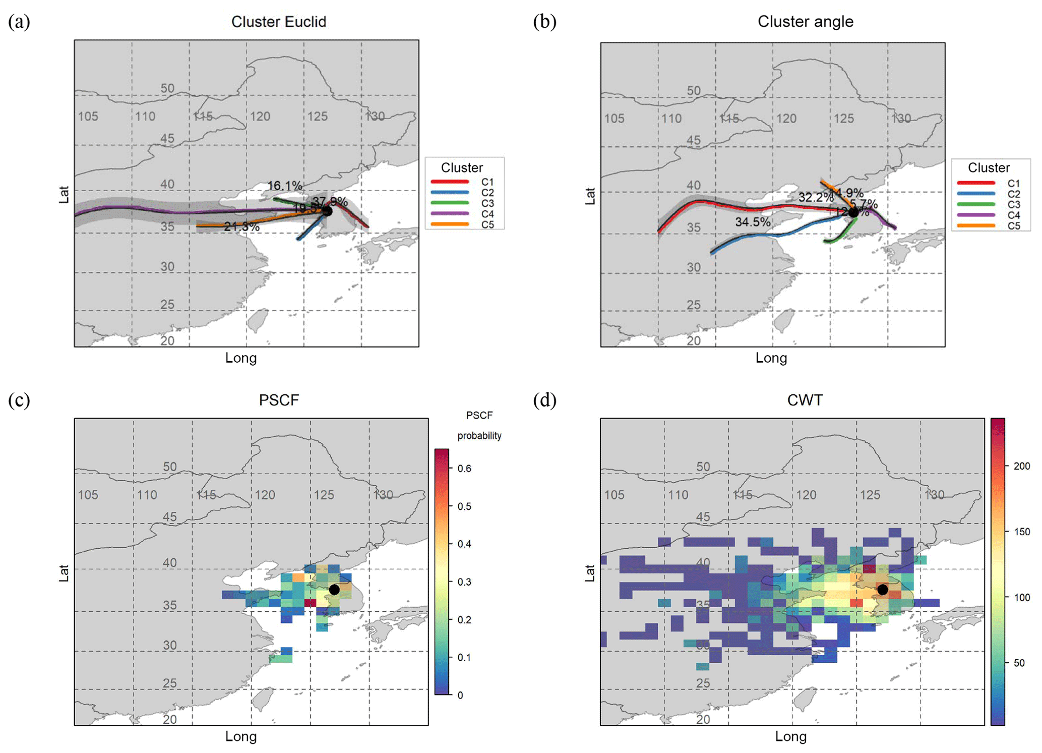
Figure 12(a) Trajectories clustered by the Euclidian distance function, (b) trajectories clustered by the angle distance function, (c) the potential source contribution factor plot, and (d) the concentration-weighted trajectory plot.
By quantifying clusters based on their trajectories, cluster analysis shows the relative importance of regional sources. Nevertheless, they are not completely accurate at determining the relative contribution of potential source regions because they do not consider concentrations together with trajectories. One method of calculating the probability of potential sources is the potential source contribution function (PSCF), which finds the probability that a source is located at a specific latitude and longitude (Pekney et al., 2006). Figure 12c shows that the probability of packets with high concentrations (i.e., those with concentrations at or above 90 percentile) passing over the Yellow Sea and reaching the SMA from the southwest was higher than 0.3. Two areas through which one packet containing a high concentration of pollutants passed showed high probabilities of 0.6 and 0.5. One was southwest of the SMA over the Yellow Sea and the other between North Korea and the coast of northern China over the Yellow Sea.
One important limitation of the PSCF is its complexity distinguishing between moderate and strong sources. To overcome this problem, we can apply the concentration-weighted trajectory (CWT) method to compute concentration fields for identifying strong source areas of pollutants. The CWT method, based on concentration values over each trajectory, estimates the trajectory-weighted concentration in each grid cell by averaging the sample pollutant concentrations of trajectories crossing each grid cell (). The results of CWT show close agreement with those of the PSCF. Figure 12d shows the distribution of weighted trajectory concentrations of CO surrounding the SMA in May 2016. The CWT results show that not only were the Yellow Sea and the Shandong Peninsula potential sources of high concentration over the SMA but other local sources may also have been strong sources. For example, the Pyongyang area in North Korea had a high concentration, weighted over 250 ppb, indicating a strong potential source of CO in this month. Furthermore, local regions such as those at west, east, and south of the SMA showed a strong potential source of high CO concentrations in Seoul. Among the long-distance sources, only the Shandong Peninsula and some parts of northern China had CO concentrations of around 100 ppmv according to the CWT analysis. As other long-distance sources were not strong sources because of the scarcity of trajectories in these areas, we consider them rare sources. For instance, although the LRT explained the high CO concentrations over the SMA during the extreme pollution period (25–28 May), during longer periods (e.g., 1 month or 1 year), with a similar contribution, distant regions from the SMA may not have been strong sources.
In this study, we introduced C-TRAIL Lagrangian output, extracted from the Eulerian CMAQ model. The comprehensive output of C-TRAIL directly linked the trajectories of pollution from the source to the receptor. We used concentration and trajectory values of C-TRAIL outputs to investigate the pollution status of originated air masses by classifying the outputs from May 2016 over East Asia into separate categories. Unlike the conventional Eulerian CO concentration plots for separate periods, which did not exhibit a clear relationship between the source and the receptor, the C-TRAIL outputs, which combined trajectories and concentrations, more vividly determined the impact of LRT on pollution during the EPP. Furthermore, during the dynamic weather period, C-TRAIL outputs showed that polluted packets from the Shandong Peninsula were responsible for high CO concentrations. The outputs for the SP revealed CO concentrations of less than 100 ppbv for distant packets, strong evidence supporting the link between local trajectories and CO concentrations over the SMA during this period.
More comprehensive investigations on C-TRAIL outputs found that the Shandong Peninsula, local regions near the SMA, and the Pyongyang area were potentially strong sources of CO pollutants during the entire month of May 2016. Overall, by analyzing the trajectory paths of packets that reached specific locations, we were able to generalize that C-TRAIL represents a practical tool for ascertaining the impact of long-range transport on species concentrations over a receptor by simultaneously providing concentrations and trajectories. C-TRAIL can be applied to LRT-impacted regions such as East Asia, North America, and India. Owing to uncertainties inherent in emission inventories and immature diffusion modeling methods, however, C-TRAIL outputs may have limitations that we will address in future work. The objective of this study is to suggest an effective tool for establishing a link between real sources of pollution to a receptor via trajectory analysis. The results of this study over East Asia showed the reliability and various advantages of C-TRAIL output. Therefore, because of its capability to determine the trajectories of masses of CO concentrations, C-TRAIL output could prove to be a highly useful tool for those who model air quality over a specific region and investigate sources of polluted air masses.
The C-TRAIL version 1.0 is derived from CMAQ v5.2 model. The CMAQ model is an open-source model which can be accessed via Zenodo (https://doi.org/10.5281/zenodo.1167892, US EPA Office of Research and Development, 2017). The documentations and tutorials on CMAQ are available on the US EPA modeling website https://www.cmascenter.org/ (last access: June 2020) and https://doi.org/10.5281/zenodo.1167892 (US EPA Office of Research and Development, 2017). The C-TRAIL v1.0 model source code and pre/post-processing scripts are available via Zenodo (https://doi.org/10.5281/zenodo.3885782, Pouyaei, 2020). The flight observations used for evaluation of the model were downloaded from the KORUS-AQ website https://www-air.larc.nasa.gov/missions/korus-aq/ (last access: June 2020) and https://doi.org/10.5067/Suborbital/KORUSAQ/DATA01 (KORUS-AQ, 2020), DC8 aircraft observations for CO comparison and ozonesonde data for wind speed/direction evaluation. For surface concentration evaluations, we used surface observational data from the Air Quality Monitoring Station (AQMS) network operated by the National Institute of Environmental Research (NIER), which is available for public on https://www.airkorea.or.kr/web (National Institute of Environmental Research, 2020).
The supplement related to this article is available online at: https://doi.org/10.5194/gmd-13-3489-2020-supplement.
AP, YC, and BS contributed to the design and implementation of the research. JJ prepared the CMAQ model and inputs. AP prepared the C-TRAIL model, analyzed the results, and took the lead in writing the paper. YC and CHS supervised the project. All authors discussed the results and commented on the paper and contributed to the final version of the paper.
The authors declare that they have no conflict of interest.
We wish to acknowledge Peter B. Percell for his technical support in the development of CMAQ-TG in this research.
This study was funded by the National Strategic Project-Fine particle of the National Research Foundation of Korea (NRF) funded by the Ministry of Science and ICT (MSIT), the Ministry of Environment (ME), and the Ministry of Health and Welfare (MOHW) (grant no. NRF-2017M3D8A1092022).
This paper was edited by Volker Grewe and reviewed by two anonymous referees.
Al-Saadi, J., Carmichael, G., Crawford, J., Emmons, L., Kim, S., Song, C.-K., Chang, L.-S., Lee, G., Kim, J., and Park, R.: KORUS-AQ: An International Cooperative Air Quality Field Study in Korea (2016), available at: https://espo.nasa.gov/korus-aq/content/KORUS-AQ (last access: June 2020), 2016.
Bertschi, I. T. and Jaffe, D. A.: Long-range transport of ozone, carbon monoxide, and aerosols to the NE Pacific troposphere during the summer of 2003: Observations of smoke plumes from Asian boreal fires, J. Geophys. Res.-Atmos., 110, 1–14, https://doi.org/10.1029/2004JD005135, 2005.
Byun, D. and Schere, K. L.: Review of the governing equations, computational algorithms, and other components of the models-3 Community Multiscale Air Quality (CMAQ) modeling system, Appl. Mech. Rev., 59, 51–76, https://doi.org/10.1115/1.2128636, 2006.
Carroll, M., Ocko, I. B., McNeal, F., Weremijewicz, J., Hogg, A. J., Opoku, N., Bertman, S. B., Neil, L., Fortner, E., Thornberry, T., Town, M. S., Yip, G., and Yageman, L.: An Assessment of Forest Pollutant Exposure Using Back Trajectories, Anthropogenic Emissions, and Ambient Ozone and Carbon Monoxide Measurements, American Geophysical Union Fall Meeting, San Fransisco, CA, USA,15–19 December 2008, Abstr. ID A41H-0227, 2008.
Carslaw, D. C. and Ropkins, K.: openair - An R package for air quality data analysis, Environ. Model. Softw., 27–28, 52–61, https://doi.org/10.1016/j.envsoft.2011.09.008, 2012.
Chen, T. F., Chang, K. H., and Tsai, C. Y.: Modeling direct and indirect effect of long range transport on atmospheric PM2.5 levels, Atmos. Environ., 89, 1–9, https://doi.org/10.1016/j.atmosenv.2014.01.065, 2014.
Chock, D. P., Sun, P., and Winkler, S. L.: Trajectory-grid: An accurate sign-preserving advection-diffusion approach for air quality modeling, Atmos. Environ., 30, 857–868, https://doi.org/10.1016/1352-2310(95)00332-0, 1996.
Chock, D. P., Whalen, M. J., Winkler, S. L., and Sun, P.: Implementing the trajectory-grid transport algorithm in an air quality model, Atmos. Environ., 39, 4015–4023, https://doi.org/10.1016/j.atmosenv.2005.03.037, 2005.
Choi, J., Park, R. J., Lee, H. M., Lee, S., Jo, D. S., Jeong, J. I., Henze, D. K., Woo, J. H., Ban, S. J., Lee, M. Do, Lim, C. S., Park, M. K., Shin, H. J., Cho, S., Peterson, D., and Song, C. K.: Impacts of local vs. trans-boundary emissions from different sectors on PM2.5 exposure in South Korea during the KORUS-AQ campaign, Atmos. Environ., 203, 196–205, https://doi.org/10.1016/j.atmosenv.2019.02.008, 2019.
Choi, S. H., Ghim, Y. S., Chang, Y. S., and Jung, K.: Behavior of particulate matter during high concentration episodes in Seoul, Environ. Sci. Pollut. Res., 21, 5972–5982, https://doi.org/10.1007/s11356-014-2555-y, 2014.
Chuang, M. T., Fu, J. S., Jang, C. J., Chan, C. C., Ni, P. C., and Lee, C. Te: Simulation of long-range transport aerosols from the Asian Continent to Taiwan by a Southward Asian high-pressure system, Sci. Total Environ., 406, 168–179, https://doi.org/10.1016/j.scitotenv.2008.07.003, 2008.
Chuang, M. T., Lee, C. Te and Hsu, H. C.: Quantifying PM2.5 from long-range transport and local pollution in Taiwan during winter monsoon: An efficient estimation method, J. Environ. Manage., 227, 10–22, https://doi.org/10.1016/j.jenvman.2018.08.066, 2018.
Cristofanelli, P., Bonasoni, P., Carboni, G., Calzolari, F., Casarola, L., Zauli Sajani, S., and Santaguida, R.: Anomalous high ozone concentrations recorded at a high mountain station in Italy in summer 2003, Atmos. Environ., 41, 1383–1394, https://doi.org/10.1016/j.atmosenv.2006.10.017, 2007.
Döös, K., Jönsson, B., and Kjellsson, J.: Evaluation of oceanic and atmospheric trajectory schemes in the TRACMASS trajectory model v6.0, Geosci. Model Dev., 10, 1733–1749, https://doi.org/10.5194/gmd-10-1733-2017, 2017.
Draxler, R. R.: An overview of the HYSPLIT_4 modelling system for trajectories, dispersion and deposition, Aust. Meteorol. Mag., 47, 295–308, 1998.
Eslami, E., Salman, A. K., Choi, Y., Sayeed, A., and Lops, Y.: A data ensemble approach for real-time air quality forecasting using extremely randomized trees and deep neural networks, Neural Comput. Appl., 32, 7563–7579, https://doi.org/10.1007/s00521-019-04287-6, 2019.
Gratz, L. E., Jaffe, D. A., and Hee, J. R.: Causes of increasing ozone and decreasing carbon monoxide in springtime at the Mt. Bachelor Observatory from 2004 to 2013, Atmos. Environ., 109, 323–330, https://doi.org/10.1016/j.atmosenv.2014.05.076, 2015.
Halliday, H. S., DiGangi, J. P., Choi, Y., Diskin, G. S., Pusede, S. E., Rana, M., Nowak, J. B., Knote, C., Ren, X., He, H., Dickerson, R. R., and Li, Z.: Using Short-Term CO/CO2 Ratios to Assess Air Mass Differences over the Korean Peninsula during KORUS-AQ , J. Geophys. Res.-Atmos., 124, 1–22, https://doi.org/10.1029/2018jd029697, 2019.
Heald, C. C., Jacob, D. J., Fiore, A. M., Emmons, L. K., Gille, J. C., Deeter, M. N., Warner, J., Edwards, D. P., Crawford, J. H., Hamlin, A. J., Sachse, G. W., Browell, E. V., Avery, M. A., Vay, S. A., Westberg, D. J., Blake, D. R., Singh, H. B., Sandholm, S. T., Talbot, R. W., and Fuelberg, H. E.: Asian outflow and trans-Pacific transport of carbon monoxide and ozone pollution: An integrated satellite, aircraft, and model perspective, J. Geophys. Res.-Atmos., 108, 4804, https://doi.org/10.1029/2003jd003507, 2003.
Hu, Y. and Talat Odman, M.: A comparison of mass conservation methods for air quality models, Atmos. Environ., 42, 8322–8330, https://doi.org/10.1016/j.atmosenv.2008.07.042, 2008.
Jeon, W., Choi, Y., Percell, P., Souri, A. H., Song, C.-K., Kim, S.-T., and Kim, J.: Computationally efficient air quality forecasting tool: implementation of STOPS v1.5 model into CMAQ v5.0.2 for a prediction of Asian dust, Geosci. Model Dev., 9, 3671–3684, https://doi.org/10.5194/gmd-9-3671-2016, 2016.
Jung, J., Souri, A. H., Wong, D. C., Lee, S., Jeon, W., Kim, J., and Choi, Y.: The Impact of the Direct Effect of Aerosols on Meteorology and Air Quality Using Aerosol Optical Depth Assimilation During the KORUS-AQ Campaign, J. Geophys. Res.-Atmos., 124, 8303–8319, https://doi.org/10.1029/2019jd030641, 2019.
Kain, J. S.: The Kain–Fritsch convective parameterization: An update, J. Appl. Meteorol., 43, 170–181, https://doi.org/10.1175/1520-0450(2004)043<0170:TKCPAU>2.0.CO;2, 2004.
KORUS-AQ: An International Cooperative Air Quality Field Study in Korea, https://doi.org/10.5067/Suborbital/KORUSAQ/DATA01, 2020.
Kruse, S., Gerdes, A., Kath, N. J., and Herzschuh, U.: Implementing spatially explicit wind-driven seed and pollen dispersal in the individual-based larch simulation model: LAVESI-WIND 1.0, Geosci. Model Dev., 11, 4451–4467, https://doi.org/10.5194/gmd-11-4451-2018, 2018.
Lee, S., Ho, C. H., and Choi, Y. S.: High-PM10 concentration episodes in Seoul, Korea: Background sources and related meteorological conditions, Atmos. Environ., 45, 7240–7247, https://doi.org/10.1016/j.atmosenv.2011.08.071, 2011.
Lee, S., Ho, C. H., Lee, Y. G., Choi, H. J., and Song, C. K.: Influence of transboundary air pollutants from China on the high-PM10 episode in Seoul, Korea for the period October 16–20, 2008, Atmos. Environ., 77, 430–439, https://doi.org/10.1016/j.atmosenv.2013.05.006, 2013.
Lee, S., Kim, J., Choi, M., Hong, J., Lim, H., Eck, T. F., Holben, B. N., Ahn, J. Y., Kim, J., and Koo, J. H.: Analysis of long-range transboundary transport (LRTT) effect on Korean aerosol pollution during the KORUS-AQ campaign, Atmos. Environ., 204, 53–67, https://doi.org/10.1016/j.atmosenv.2019.02.020, 2019.
Li, M., Zhang, Q., Kurokawa, J.-I., Woo, J.-H., He, K., Lu, Z., Ohara, T., Song, Y., Streets, D. G., Carmichael, G. R., Cheng, Y., Hong, C., Huo, H., Jiang, X., Kang, S., Liu, F., Su, H., and Zheng, B.: MIX: a mosaic Asian anthropogenic emission inventory under the international collaboration framework of the MICS-Asia and HTAP, Atmos. Chem. Phys., 17, 935–963, https://doi.org/10.5194/acp-17-935-2017, 2017.
Liu, Y., Xu, S., Ling, T., Xu, L., and Shen, W.: Heme oxygenase/carbon monoxide system participates in regulating wheat seed germination under osmotic stress involving the nitric oxide pathway, J. Plant Physiol., 167, 1371–1379, https://doi.org/10.1016/j.jplph.2010.05.021, 2010.
Lops, Y., Choi, Y., Eslami, E., and Sayeed, A.: Real-time 7-day forecast of pollen counts using a deep convolutional neural network, Neural Comput. Appl., 32, 1–10, https://doi.org/10.1007/s00521-019-04665-0, 2019.
Miyazaki, K., Sekiya, T., Fu, D., Bowman, K. W., Kulawik, S. S., Sudo, K., Walker, T., Kanaya, Y., Takigawa, M., Ogochi, K., Eskes, H., Boersma, K. F., Thompson, A. M., Gaubert, B., Barre, J., and Emmons, L. K.: Balance of Emission and Dynamical Controls on Ozone During the Korea-United States Air Quality Campaign From Multiconstituent Satellite Data Assimilation, J. Geophys. Res.-Atmos., 124, 387–413, https://doi.org/10.1029/2018JD028912, 2019.
National Institute of Environmental Research: available at: https://www.airkorea.or.kr/web, last access: June 2020.
Oh, H. R., Ho, C. H., Kim, J., Chen, D., Lee, S., Choi, Y. S., Chang, L. S., and Song, C. K.: Long-range transport of air pollutants originating in China: A possible major cause of multi-day high-PM10 episodes during cold season in Seoul, Korea, Atmos. Environ., 109, 23–30, https://doi.org/10.1016/j.atmosenv.2015.03.005, 2015.
Pekney, N. J., Davidson, C. I., Zhou, L., and Hopke, P. K.: Application of PSCF and CPF to PMF-Modeled Sources of PM2.5 in Pittsburgh, Aerosol Sci. Technol., 40, 952–961, https://doi.org/10.1080/02786820500543324, 2006.
Petetin, H., Beekmann, M., Sciare, J., Bressi, M., Rosso, A., Sanchez, O., and Ghersi, V.: A novel model evaluation approach focusing on local and advected contributions to urban PM2.5 levels – application to Paris, France, Geosci. Model Dev., 7, 1483–1505, https://doi.org/10.5194/gmd-7-1483-2014, 2014.
Pouyaei, A.: armanpouyaei/C-TRAIL-v1.0: First release (Version 1.0), Zenodo, https://doi.org/10.5281/zenodo.3885782, 2020.
Price, H. U., Jaffe, D. A., Cooper, O. R., and Doskey, P. V.: Photochemistry, ozone production, and dilution during long-range transport episodes from Eurasia to the northwest United States, J. Geophys. Res.-Atmos., 109, 1–10, https://doi.org/10.1029/2003JD004400, 2004.
Pu, W., Zhao, X., Shi, X., Ma, Z., Zhang, X., and Yu, B.: Impact of long-range transport on aerosol properties at a regional background station in Northern China, Atmos. Res., 153, 489–499, https://doi.org/10.1016/j.atmosres.2014.10.010, 2015.
Rößler, T., Stein, O., Heng, Y., Baumeister, P., and Hoffmann, L.: Trajectory errors of different numerical integration schemes diagnosed with the MPTRAC advection module driven by ECMWF operational analyses, Geosci. Model Dev., 11, 575–592, https://doi.org/10.5194/gmd-11-575-2018, 2018.
Sadeghi, B., Choi, Y., Yoon, S., Flynn, J., Kotsakis, A., and Lee, S.: The characterization of fine particulate matter downwind of Houston: Using integrated factor analysis to identify anthropogenic and natural sources, Environ. Pollut., 262, 114345, https://doi.org/10.1016/j.envpol.2020.114345, 2020.
Salvador, P., Artíñano, B., Querol, X., and Alastuey, A.: A combined analysis of backward trajectories and aerosol chemistry to characterise long-range transport episodes of particulate matter: The Madrid air basin, a case study, Sci. Total Environ., 390, 495–506, https://doi.org/10.1016/j.scitotenv.2007.10.052, 2008.
Sarwar, G., Simon, H., Bhave, P., and Yarwood, G.: Examining the impact of heterogeneous nitryl chloride production on air quality across the United States, Atmos. Chem. Phys., 12, 6455–6473, https://doi.org/10.5194/acp-12-6455-2012, 2012.
Sayeed, A., Choi, Y., Eslami, E., Lops, Y., Roy, A., and Jung, J.: Using a deep convolutional neural network to predict 2017 ozone concentrations, 24 hours in advance, Neural Networks, 121, 396–408, https://doi.org/10.1016/j.neunet.2019.09.033, 2020.
Souri, A. H., Choi, Y., Li, X., Kotsakis, A., and Jiang, X.: A 15-year climatology of wind pattern impacts on surface ozone in Houston, Texas, Atmos. Res., 174–175, 124–134, https://doi.org/10.1016/j.atmosres.2016.02.007, 2016.
Stenke, A., Dameris, M., Grewe, V., and Garny, H.: Implications of Lagrangian transport for simulations with a coupled chemistry-climate model, Atmos. Chem. Phys., 9, 5489–5504, https://doi.org/10.5194/acp-9-5489-2009, 2009.
Stohl, A.: Trajectory statistics – A new method to establish source-receptor relationships of air pollutants and its application to the transport of particulate sulfate in Europe, Atmos. Environ., 30, 579–587, https://doi.org/10.1016/1352-2310(95)00314-2, 1996.
Stohl, A.: Computation, accuracy and applications of trajectories – a review and bibliography, Dev. Environm. Sci., 1, 615–654, https://doi.org/10.1016/S1474-8177(02)80024-9, 2002.
Stohl, A. and Seibert, P.: Accuracy of trajectories as determined from the conservation of meteorological tracers, Q. J. Roy. Meteor. Soc., 124, 1465–1484, https://doi.org/10.1002/qj.49712454907, 1998.
US EPA Office of Research and Development: CMAQ (Version 5.2), Zenodo, https://doi.org/10.5281/zenodo.1167892, 2017.
Vay, S. A., Choi, Y., Vadrevu, K. P., Blake, D. R., Tyler, S. C., Wisthaler, A., Hecobian, A., Kondo, Y., Diskin, G. S., Sachse, G. W., Woo, J. H., Weinheimer, A. J., Burkhart, J. F., Stohl, A., and Wennberg, P. O.: Patterns of CO2 and radiocarbon across high northern latitudes during International Polar Year 2008, J. Geophys. Res.-Atmos., 116, 1–22, https://doi.org/10.1029/2011JD015643, 2011.
Wang, F., Chen, D. S., Cheng, S. Y., Li, J. B., Li, M. J., and Ren, Z. H.: Identification of regional atmospheric PM10 transport pathways using HYSPLIT, MM5-CMAQ and synoptic pressure pattern analysis, Environ. Model. Softw., 25, 927–934, https://doi.org/10.1016/j.envsoft.2010.02.004, 2010.
Weiss-Penzias, P., Jaffe, D. A., Jaeglé, L., and Liang, Q.: Influence of long-range-transported pollution on the annual and diurnal cycles of carbon monoxide and ozone at Cheeka Peak Observatory, J. Geophys. Res.-Atmos., 109, 1–15, https://doi.org/10.1029/2004JD004505, 2004.
Xu, S., Warner, N., Bohlin-Nizzetto, P., Durham, J., and McNett, D.: Long-range transport potential and atmospheric persistence of cyclic volatile methylsiloxanes based on global measurements, Chemosphere, 228, 460–468, https://doi.org/10.1016/j.chemosphere.2019.04.130, 2019.
Zhang, Q., Xue, D., Liu, X., Gong, X., and Gao, H.: Process analysis of PM2.5 pollution events in a coastal city of China using CMAQ, J. Environ. Sci. (China), 79, 225–238, https://doi.org/10.1016/j.jes.2018.09.007, 2019.
- Abstract
- Introduction
- Methodology
- Setup and validation of the model
- Analysis of C-TRAIL
- Case study for the C-TRAIL analysis: the May 2016 KORUS-AQ period
- Conclusions
- Code and data availability
- Author contributions
- Competing interests
- Acknowledgements
- Financial support
- Review statement
- References
- Supplement
packetsof species along trajectories determined by the wind field.
- Abstract
- Introduction
- Methodology
- Setup and validation of the model
- Analysis of C-TRAIL
- Case study for the C-TRAIL analysis: the May 2016 KORUS-AQ period
- Conclusions
- Code and data availability
- Author contributions
- Competing interests
- Acknowledgements
- Financial support
- Review statement
- References
- Supplement