the Creative Commons Attribution 4.0 License.
the Creative Commons Attribution 4.0 License.
 | 23 Jul 2020
Simple algorithms to compute meridional overturning and barotropic streamfunctions on unstructured meshes
Sergey Danilov
Nikolay Koldunov
Patrick Scholz
Qiang Wang
Computation of barotropic and meridional overturning streamfunctions for models formulated on unstructured meshes is commonly preceded by interpolation to a regular mesh. This operation destroys the original conservation, which can be then artificially imposed to make the computation possible. An elementary method is proposed that avoids interpolation and preserves conservation in a strict model sense. The method is described as applied to the discretization of the Finite volumE Sea ice – Ocean Model (FESOM2) on triangular meshes. It, however, is generalizable to colocated vertex-based discretization on triangular meshes and to both triangular and hexagonal C-grid discretizations.
- Article
(7943 KB) - Full-text XML
- BibTeX
- EndNote


Over recent years, a considerable progress has been achieved in the development of global ocean circulation models working on horizontally unstructured meshes such as FESOM1.4 (Wang et al., 2014), MPAS-Ocean (Ringler et al., 2013), FESOM2 (Danilov et al., 2017) and ICON-Ocean (Korn, 2017). By refining in dedicated areas of the world ocean, these models may resolve dynamics that would otherwise require nesting or using a higher resolution globally. Since these models still use vertically aligned meshes, the overhead of horizontally unstructured mesh is minimized because the horizontal neighborhood information is valid for the entire vertical column and becomes negligible as the number of vertical levels is increased. These models show a very good parallel scalability and reach throughput (in simulated years per day) comparable to that of structured-mesh models (Koldunov et al., 2019). However, the unstructured character of meshes makes many traditional diagnostics, such as barotropic and meridional overturning streamfunctions, difficult. Any interpolation on a regular mesh violates the sense in which continuity is satisfied in a model and introduces errors which, while often acceptable for computing local fluxes and transports, are very annoying in computations of global or basin streamfunctions where large positive and negative contributions are combined together. Furthermore, in the case of streamfunctions, one is most frequently interested in variability, which might be easily masked or biased by the inconsistencies introduced by the analysis procedure. In the early version of FESOM, based on continuous finite elements, the situation was exacerbated by continuity being formulated in a weighted sense, without explicitly computed fluxes (Sidorenko et al., 2009).
All new large-scale ocean models are based on the finite-volume method and as such have a clear definition of fluxes at boundaries of the control cells of their meshes. However, these fluxes are defined on irregularly located faces, so instead of using them in their original sense, one is tempted to rely on interpolation to a regular mesh. Our practice shows that incurred inconsistencies can be large, and this road should not be followed if global or basin-scale quantities are computed. It turns out that there are efficient and easy-to-implement procedures that are based on exact fluxes and balances and that might be used for analyses. These procedures do not rely on interpolation but use binning, which is sufficient in most cases except for very coarse meshes. The intention of this note is to describe some of them. In doing so we will use the arrangement of variables of FESOM2; however the adjustments needed for other models with different discretizations are relatively straightforward and will be briefly mentioned. We suspect that similar procedures are already used by other groups – in particular, for the analysis on cubed-sphere meshes of the Massachusetts Institute of Technology general circulation model see, e.g., Adcroft et al. (2004), tripole grid configurations of Parallel Ocean Program (POP; Smith and Gent, 2004) or MPAS-Ocean – but we feel that they need to be documented for unstructured meshes, facilitating the use of unstructured-mesh models by a broader community.
We will discuss computations of meridional overturning streamfunctions in height and density coordinates as well as computations of barotropic streamfunctions.
FESOM2 uses a cell–vertex discretization, placing horizontal velocities on centroids of triangles and scalar quantities at vertices if viewed from the surface, as shown schematically in Fig. 1. These quantities are stored at midlevels. Vertical velocities are located at vertices and full levels. We use index v to enumerate vertices, c (cells) to enumerate triangles, and k to enumerate vertical levels or midlevels (centers of layers). The velocity control volumes are mesh triangles, and scalars are associated with median-dual control volumes formed in the horizontal plane by connecting midpoints of edges with cell centroids. On uniform equilateral meshes they coincide with hexagons of the dual mesh, but in the general case they differ. For the reasons discussed in Danilov et al. (2017) the bottom topography of FESOM is given on cells, implying that velocity control volumes are triangular prisms in 3D. However, a part of scalar control volume can be cut by bottom topography at depths, and its footprint will differ from that at the surface. As a consequence, there is a 1D array Ac of triangle areas and a 2D array Akv of the areas of scalar control volumes. The transport through the top face of scalar prism with indices (k,v) is wkvAkv, with wkv the respective vertical (or cross-level in the case of moving level surfaces) velocity. Each triangle is characterized by the list of its vertices v(c), which is for c=c1 in Fig. 1.
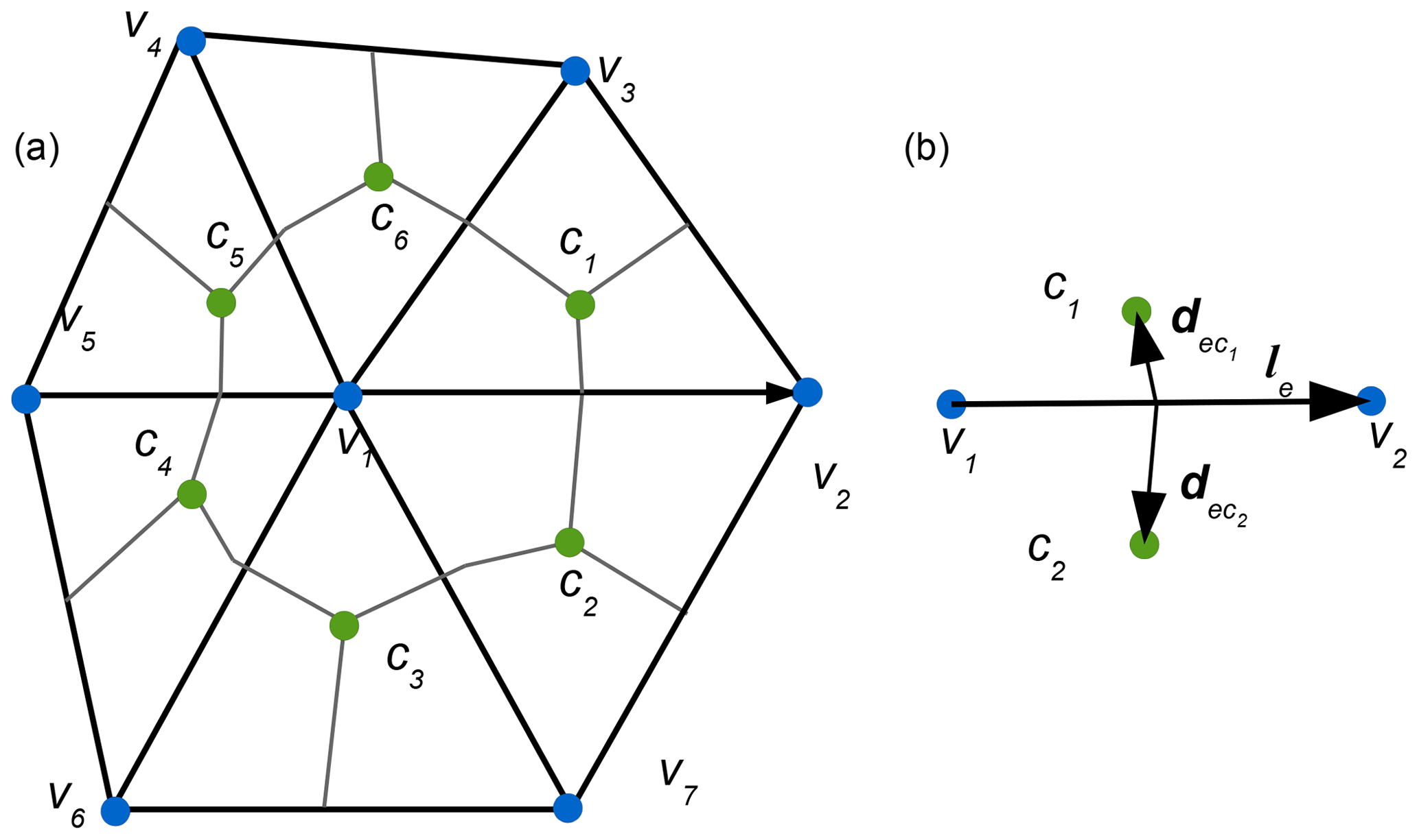
Figure 1Horizontal schematic of (a) median-dual control volumes and the (b) edge-based structure. In FESOM2, scalar quantities and vertical velocity are at vertices (blue circles), while the horizontal velocities are at triangle centroids (green circles). The median-dual control volume around vertex v1 is bounded by segments (gray lines) connecting the centers of neighbor triangles with midpoints of edges. Edge e in (b) is characterized by its vertices and cells with c1 on the left. The edge vector le connects vertex v1 to vertex v2. The edge cross vectors and connect the edge midpoint to the respective cell centers.
The elementary structure used in computations of horizontal fluxes between two scalar control volumes is given by mesh edges (labeled with index e). An edge is characterized by its two vertices (v1,v2) symbolically written as v(e) and two cells it belongs to, (c1,c2) symbolically written as c(e). For boundary edges c2 is absent, and c1 is the left cell to the edge direction, which is from the edge first vertex to the second one. There are two vectors drawn from edge midpoint to centroids of edge cells, . Their components are expressed in local Cartesian coordinates related to respective cells. The transport through the faces of the scalar control volume in layer k in the direction of the edge is
where ez is a unit vertical vector, and are the layer thicknesses at respective velocity points, and Te is the tracer estimate at edge midpoint. Te=1 for volume transport. In MPAS-Ocean or ICON-Ocean codes, which are based on hexagonal and triangular C-grid discretizations, normal velocities are located at edges and computations of transports are simpler. The arrangement of hexagonal C grid is easily obtained from the case considered here if edges of dual triangular mesh are considered (with the difference that centroids are replaced by circumcenters and lines connecting c1 with c2 are perpendicular to edge “e”). Importantly, edge-related transports are the same as in the model; however care should also be taken that Te is computed in the same way as in the model if fluxes are to be properly analyzed.
For zonally integrated vertical and meridional velocities and of a divergence-less flow we can introduce (see, e.g., Kundu et al., 2012) a streamfunction Ψ(z,θ) such that
Here θ is the latitude in radians, z is the depth, RE is Earth's radius, v and w are the meridional and vertical velocities and xw and xe the western and eastern boundaries in zonal direction. Following the definition, there are two convenient ways of computing global Ψ in geopotential coordinates:
or
Here θr is the reference latitude. For global meridional overturning circulation (MOC) computations it is the southernmost latitude of the Antarctic coast, where . For regional MOCs, like the Atlantic MOC (AMOC), θr is any convenient latitude where should be provided. For this, the Eq. (4) is usually used. In this equation the boundary condition is naturally taken into account by integrating from the bottom . Note that both ways of computation are equivalent because the full velocity vector is divergence-free. In the following we discuss details of both methods of computation on unstructured meshes. Method A (Eq. 3) involves vertical velocities and is more straightforward. Method B (Eq. 4) is based on horizontal velocities and is slightly more complicated.
3.1 Method A
In FESOM2, the vertical velocity is conservatively remapped from vertices to cells using
where v(c) is the list of vertices of triangle c and Nc is the number of the bottom level on triangle c. Indeed, it is easy to prove that for FESOM2 discretization, so that the vertical (across level surface) transport is preserved. Using triangles is more convenient in FESOM2 because bottom depth is constant on triangles. This remapping is not required in ICON-Ocean and MPAS-Ocean where the bottom depth is specified at scalar locations.
We introduce a set of latitude bins , , , covering the ocean domain. The computational procedure is straightforward and is illustrated schematically in Fig. 2.
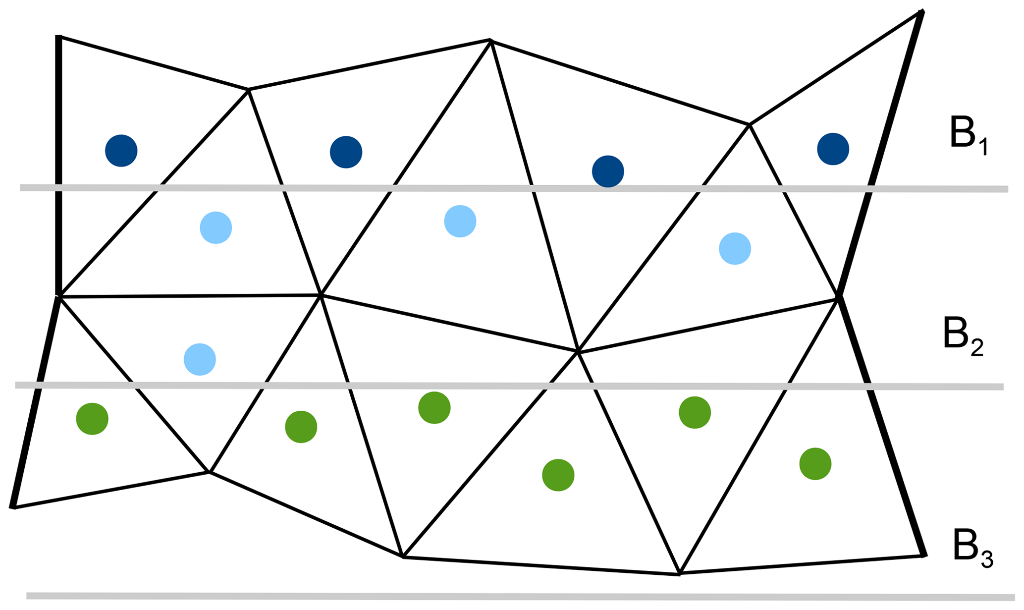
Figure 2Schematic of binning. Circles correspond to triangle centroids. Bins (here B1, B2 and B3) are given by selected latitude lines. A triangle is in a bin if its centroid is in this bin. Triangles with centroids in dark blue, light blue and green fit in bins B1, B2 and B3, respectively.
-
For each bin i find the list of triangles c(i) with centroids in these bins. They will be partly masked by bottom topography in deep layers, and we will formally write this list as c(ki), adding a layer index k. Subsequent computations are over triangles and levels, so that only c(ki) is needed.
-
Compute Δψki as
where cki is the list of triangles, the centers of which are in bin i at level k.
-
Compute the meridional overturning streamfunction
The procedure as written is strictly applicable in the case when level surfaces are fixed except for the surface. For z* vertical coordinates or for other options where level surfaces are changing only slightly around their mean positions it can still be used in most cases. It can be readily augmented with a vertical remap to fixed levels by considering that the difference in transports is linearly distributed within the layer in the case when layers do not disappear, and level surfaces do not outcrop and stay at fixed depths where they cross topography. The method B should be used in more general cases.
Generally Δθ should be taken about the same or larger than the typical size of triangles. The triangles that are counted as belonging to a bin are not necessarily confined to this bin, and the total area occupied by them differs from the bin area. However, there generally are sufficiently many triangles in each bin, and one gets a smooth Ψkj despite these effects. The procedure can be improved by conservative remapping into bins, which might be needed on coarse meshes. One may always check the bin attribution effect by repeating computations with smaller Δθ. We also note that for instantaneous vertical velocities the procedure may result in Ψ different from zero at the surface. It will become zero only upon sufficient averaging, which removes transient behavior of the surface.
The computations presented here can be generalized to some other sets of binning. Any sufficiently smooth scalar quantity defined at vertices or triangles can be used to introduce a set of bins. For example, being limited to the N Atlantic subpolar gyre, one may ask where the AMOC is forming using bins in mean sea surface height or barotropic streamfunction (see, e.g., Katsman et al., 2018).
In the following we present an example showing differences between computations using different bins in Δθ. For this, FESOM was configured on a mesh with resolution varying from a nominal 1∘ in the interior of the ocean to ∘ in the equatorial belt and ∼24 km north of 50∘ N. We run the model for 1 year starting from climatology and compute the MOC from the annually averaged velocity. Because of starting the model at rest and a short period of averaging we expect , where η is the sea surface height. This, however, shall not affect the presented results. Figure 3 depicts the simulated global MOC, which is expressed by the basin-wide, mid-depth cell of ∼20 Sv at 40∘ N and the bottom cell, induced by the circulation of the Antarctic Bottom Water with a maximum of 10 Sv. Bins with Δθ=0.125∘, which are finer than the nominal resolution, have been used for computing the streamfunction. Differences between computations using different bins in Δθ are shown in Fig. 4. Using the coarsest bin size of 4∘ the difference in MOC reaches locally above 5 Sv. As one would expect, decreasing the size of bins leads to convergence towards the solution obtained with the finest bin size of . We see that using bins of is already sufficient in this case because the mesh contains only a few triangles that are smaller than the bin size.

Figure 3Global meridional overturning circulation (MOC) streamfunction including the eddy-induced transports. Method A was used for the computation. The streamfunction depicts a canonical pattern as known from the literature with a maximum of 20 Sv at 45∘ N.
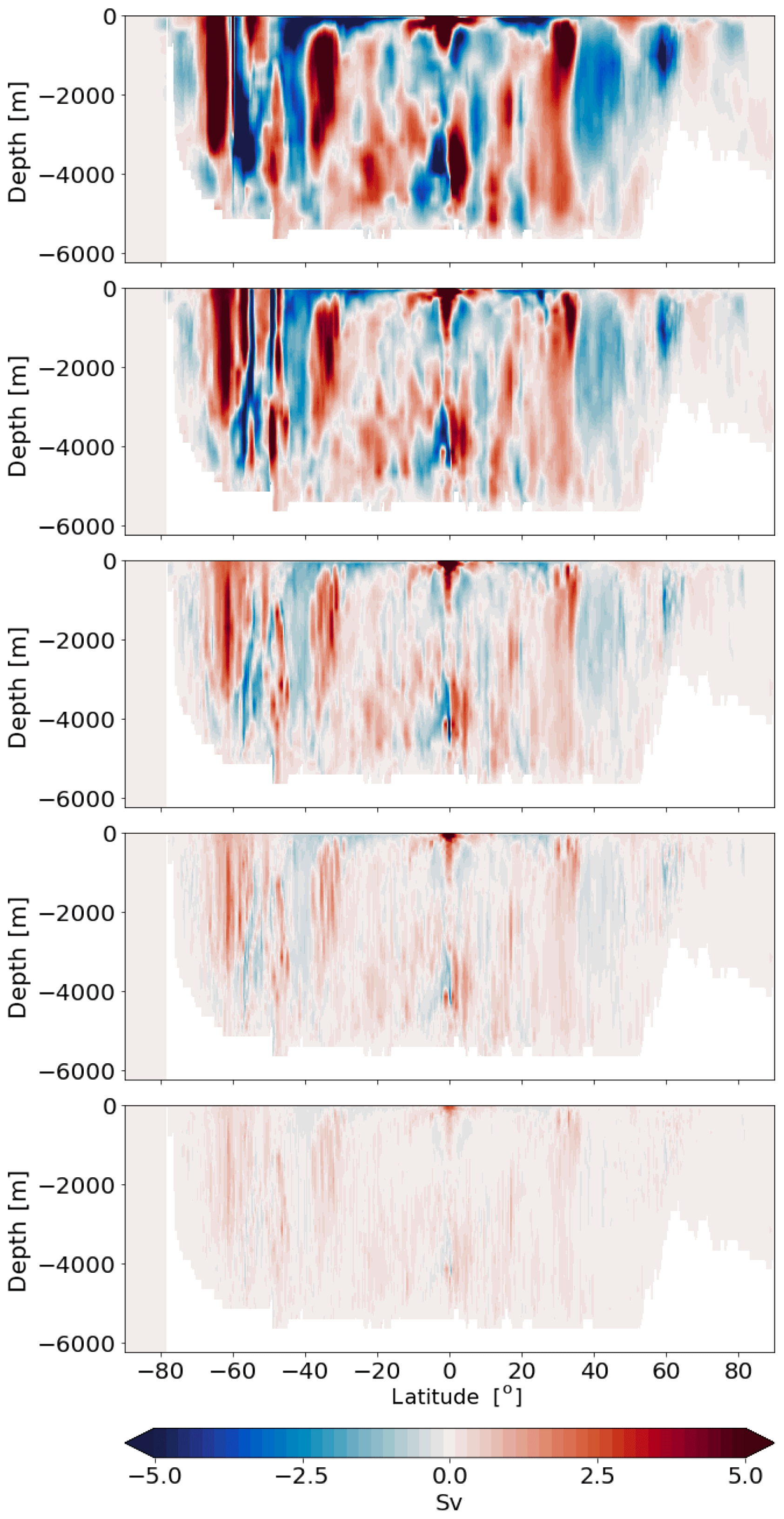
Figure 4Differences in MOC computed with method A and using bins Δθ=4∘, 2∘, 1∘, 0.5∘, 0.25∘ (from top to the bottom) relative the MOC computed with Δθ=0.125∘. Evidently there is a convergence with decreasing bin size.
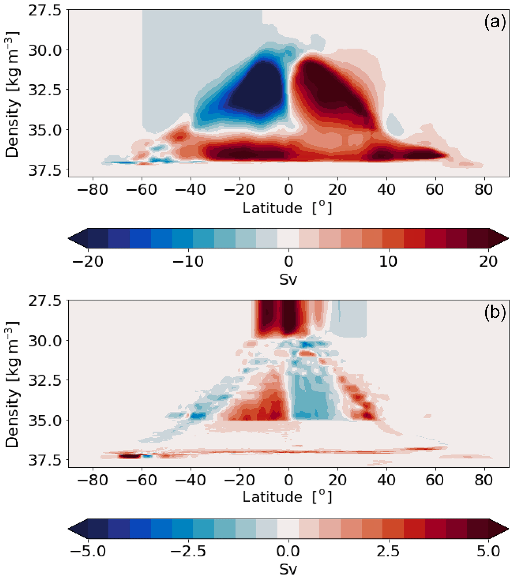
Figure 5Panel (a) shows the MOC computed using 1000 equally spaced density levels varying from 1027.5 to 1037.5 kg m−3. Panel (b) shows the difference in MOC if 72 unequally spaced vertical levels after Megann et al. (2010) are used.
3.2 Method B
Here the horizontal velocities are used. We select a set of latitudes θi. The steps of the procedure are as follows.
-
For each i, draw a line θ=θi, and find a set of edges crossed by this line, as shown schematically in Fig. 6. For this, cycle through all edges, picking up those that satisfy the condition , with and the latitudes of edge vertices. To avoid situations when the line passes exactly through the mesh vertex, a random noise of small amplitude is added to the original θi before edge e with vertices (v1,v2) is tested. The schematic in Fig. 6 shows that the actual line through which transport is computed is a broken line composed of vectors related to the crossed edges. For a triangular C-grid discretization, one will deal with transports directly through the edges. The caveat in this case is that some of the crossed edges will be hanging and not contributing to the broken line. They are excluded by noticing that they have vertices that are encountered only once in the union of vertices of crossed edges. On hexagonal C grids the procedure needs to deal with edges of dual triangular mesh. We denote the set of edges forming the broken line around θ=θi as e(i).
-
The flux associated with the edge is given by the expression for Fe above. The question now is the orientation of edges. This question is trivially solved for each “e” by taking Fe if and −Fe otherwise. It corresponds to keeping the normals to segments oriented so that transports are from the “northern” side of the broken curve. On a triangular C grid, the edge normal vectors used to introduce edge velocities can be selected as turned 90∘ in the positive direction from the edge direction. This will allow the orientation problem to be solved in the same way.
-
Since each of segments belongs to a particular cell, vertical integration is trivial for fixed level surfaces. If level surfaces are moving, the fluxes (transports) through the faces associated with segments are conservatively interpolated to the desired system of levels assuming a linear distribution within model layers. In particular, the new system of levels can be specified in terms of potential density, with the result being the streamfunction in density coordinates. For each level the contributions from edges e∈e(i) are summed to get a streamfunction at this level and the latitude θi.
Note that the set of intersected edges may be ordered arbitrarily; the computation relies on the orientation of edges with respect to lines θ=θi. This is the reason why the search for intersected edges remains relatively fast even on very large meshes. Furthermore, it needs to be done only once for a particular mesh. Similarly to method A, computations can be generalized to any set of lines, in particular to isolines of mean sea surface height or a barotropic streamfunction. In both methods we introduce masks if computations need to be confined to a particular basin.
Using this method we computed the streamfunction using the discrete spacing of Δθ=0.125∘. The difference to the streamfunction computed by method A is illustrated in Fig. 7. The discrepancy between both methods is caused by the difference of attribution of the ocean volume to θi. This, as shown in Fig. 7, can lead to a differences exceeding locally 1 Sv. These differences are not the errors but uncertainty in the interpretation (see further).
If the modeled fluxes have been remapped onto the desired set of vertical levels as, for instance, prescribed density levels, method B can be directly used for computing the MOC for a new vertical coordinate system. Figure 5 depicts the MOC computed using the σ2 (density referenced to 2000 m) coordinate in vertical. For computing the streamfunction in density coordinates, we used 1000 equally spaced σ2 levels varying from 1027.5 to 1037.5 kg m−3. The resulting MOC resembles that of generally known pattern from literature, with less expressed Deacon cells related to z-coordinate streamfunction. The result is sensitive to the selection of density bins, as illustrated in Fig. 5b where the difference is presented with computations relying on the density levels of Megann (2018). This study used 72 unequally spaced density classes spanning the range kg m−3 and used the logarithmic scale for densities higher than σ2>35.0 kg m−3 to better represent the deep and bottom waters. Thus, due to the different sampling the difference in the equatorial overturning of the surface waters reaches ∼3 Sv for kg m−3 and is even larger for the circulation cell associated with the Antarctic Bottom Water. We conclude that different or not-detailed-enough selection of density levels may result in the small-scale recirculations in the diagnosed MOC. However, this difference is not an error but attribution uncertainty created by arbitrariness in the selection of density levels.
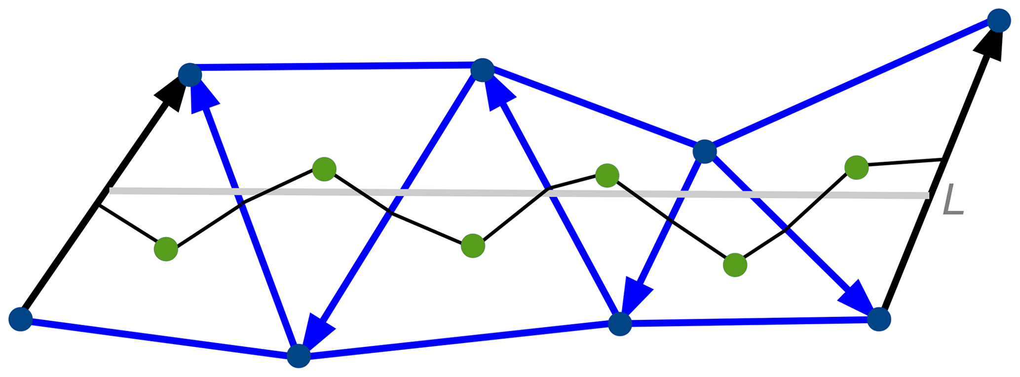
Figure 6Schematic of edge search method. The gray line L intersects edges depicted with arrows that show their orientation. The set of segments drawn to centroids from the centers of intersected edges forms a broken line connecting land at the left to land at the right where exact expressions for fluxes are available in FESOM2. The broken line formed by the intersected edges will be taken on triangular C grids, and on hexagonal C grids it will be composed of edges of primary hexagonal mesh. The set of intersected edges may stay disordered; only edge orientation with respect to the line L should be known. The latter is positive if the latitude of the first edge point is larger than that of L and negative otherwise. The transport through L is the transport through the associated broken line.
Note that the diagnostic of MOC in density coordinates can be also made in the same manner as method A. For this, the horizontal divergence needs to be remapped conservatively into density bins. From the horizontal divergence we then (1) diagnose the diapycnal velocity and (2) use it in method A.
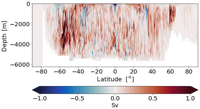
Figure 7Differences between computations of MOC using meridional (method B) or vertical (method A) velocities. The discrepancy between techniques may result in differences of more than 1 Sv.
As follows from the equation for elevation, time mean vertically integrated horizontal velocity U is divergence-free, ; i.e., it can be written in terms of the barotropic streamfunction as
This streamfunction gives vertically integrated transport between two points at the surface.
4.1 Computations through binning
The barotropic streamfunction is more difficult to compute because binning has to be done in two directions. We introduce first a set of lines ϕ=ϕj, where ϕ is the longitude and ϕj is the set of equally spaced longitude values over the basin of interest. As a first step the set of broken lines associated with each straight line ϕ=ϕj is found. As the next step, vertically integrated transports associated with the segments of broken line are computed. The final step is further binning of edges and associated transports into equally spaced latitude intervals . Transport (and hence a streamfunction) at each bin can be then computed by summing contributions going from the southern boundary where is set to zero.
This procedure can potentially be more noisy than computations of MOC and may benefit from a conservative remap of the contributions from the segments in the second binning step (the number of segments in final bins is not necessarily large, in contrast to computations of meridional overturning).
According to the above procedure we computed the barotropic streamfunction using Δθ and Δϕ=0.25∘. Considering that the procedure requires a 2-fold loop for (Δθi,Δϕj) in the case of large meshes and small bins, it can become computationally heavy. The result is illustrated in Fig. 8a and depicts reasonable structure of the main gyres with transports of 160 and 70 Sv across Antarctic Circumpolar Current (ACC) and Gulf Stream, respectively.
Fig. 8b and c show the differences between the streamfunctions if bins of 2 and 1∘, respectively, are used. As expected, the largest differences occur along the main gradients and reach above 5 Sv along the ACC front. As in the case with the MOC we note that these differences are not the errors but uncertainty created by arbitrariness in the selection of bin size.
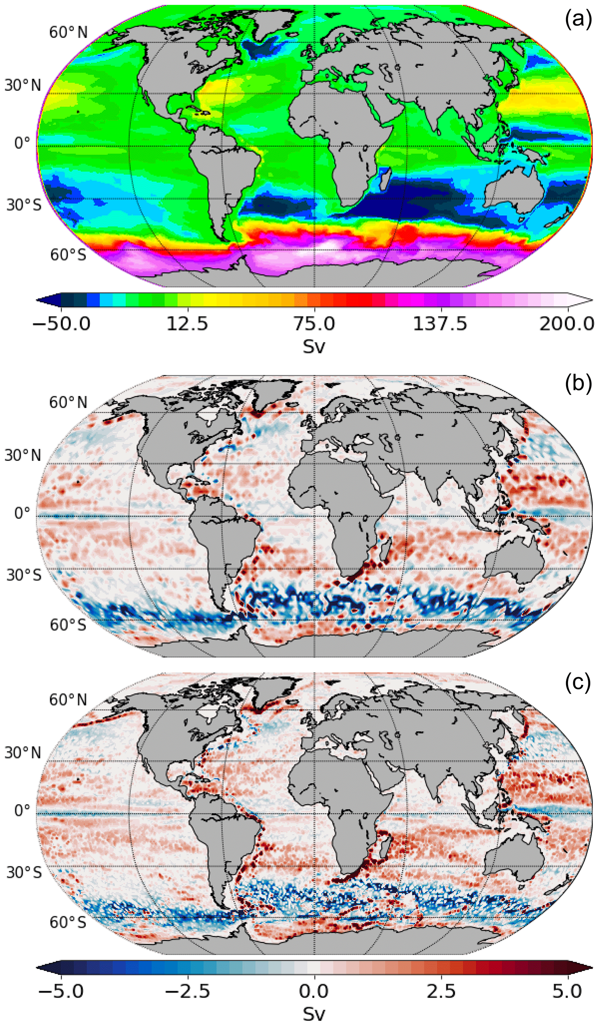
Figure 8(a) The barotropic streamfunction computed using Δθ and Δϕ=0.25∘. Panels (b) and (c) show the differences in the cases Δθ=1 and 2∘, respectively.
4.2 Computations through velocity curl
FESOM2, as its predecessor, uses implicit time stepping for the internal mode. The already available solver and routines need to be only slightly adjusted to compute the barotropic streamfunction in the case when no-slip boundary conditions are applied. Taking curl of the equation defining , one gets
In FESOM the discrete ζ is located at scalar points (at vertices), so modifications of the sea surface height solver to solve the above equations are indeed elementary. The difficulty in formal application of this approach is that the equation above needs to be solved in a multiply-connected domain with the Dirichlet boundary conditions provided on the periphery of each island and continent. Although these conditions can be formally provided by drawing lines connecting the islands and computing transports through the associated broken lines, this is tedious enough, especially when mesh resolution is high (and there are many islands). In the case of no-slip boundary conditions, circulations along each island are identically zero, and the equation above can be formally solved with the Dirichlet boundary condition on the southern boundary and the von Neumann boundary condition (n is the normal to the boundary). Although this condition does not ensure that is constant over the periphery of any island, our experience with FESOM1.4 is that it works well enough for practical purposes.
If we integrate the equation above over a scalar control volume (in FESOM2 scalar points are natural locations for relative vorticity ζ and streamfunction), we get
The contributions from edges on boundaries here are one-sided, including only segments that are wet (the first in the list in the case of FESOM). This automatically takes into account that there are no contributions from the boundary, as is the case for the no-slip boundary conditions. The operator on the left-hand side in the case of FESOM is, up to the absence of depth weighting, the same as the part of operator used to compute the elevation, so the implementations is straightforward in the code (less so for postprocessing). A clear drawback of this procedure is that it is not applicable for partial-slip boundary conditions (it can be generalized but will become too complicated). Since the methods based on bins was found to perform reliably, the curl-based method presents largely a historical interest.
The FESOM 2.0 source code is available at https://github.com/FESOM/fesom2 (last access: 8 July 2020). It is written in Fortran 90 with some C/C++ code for providing bindings to some of the third-party libraries. The code employs the distributed memory parallelization based on Message Passing Interface (MPI) to run on HPC systems. The presented diagnostics have been computed using Python routines that are part of the FESOM 2.0 code distribution. For computing the MOC in z coordinates, Python routines require either vertical or horizontal velocities to be stored as wk,v or , where k, v and c denote the layer, vertex or element indices, respectively. This is the default output provided by FESOM. For computing the MOC in density space, the index k refers to a density bin and wk,v (is then diagnosed from the horizontal divergence within the bins) or denotes the transport through this bin below the element c. Transports within the density classes are instantaneously computed by FESOM and stored with the desired frequency if option ldiag_dMOC is activated. For the sake of better subsampling, the number of density classes for computing transports shall be sufficiently large. This, however, can make the remapping of transports onto density bins computationally heavy. Our experience shows that instantaneous remapping of modeled fluxes onto density classes results in a ∼25 % slow down of the code if 80 density classes are used. For this reason ldiag_dMOC is switched off per default.
For postprocessing in Python, a combination of dask and xarray is used for reading a 3D field (if, for example, the mean over several timesteps or years is required). The MOC calculation itself happens using the data that are located in memory. One should have, of course, a sufficient amount of memory installed on the post processing machine. Our experience shows that 200 GB is enough to compute MOC for a mesh with ∼23 million surface vertices. For a mesh with ∼1.3 million surface vertices and 49 vertical levels it takes about 7 s to compute a global MOC using 91 latitudinal bins. For the largest mesh we have tested in FESOM so far (23 million surface vertices) and 80 levels in vertical, the same computation takes about 7 min.
Computation of the barotropic streamfunction is currently implemented offline, and from our experience it is slow because of loops along vertical and zonal directions are required. Hence we plan to implement the computation of the barotropic streamfunction following the philosophy of the in situ computations (see, e.g., Woodring et al., 2015).
The general idea of the simple procedures described above is the use of transports as they are defined in an unstructured-mesh model, avoiding interpolation from an unstructured to a structured mesh. The diagnosed quantities such as meridional and barotropic streamfunctions rely on the continuity equation, which is satisfied by the model only in a certain discrete sense. Interpolation destroys this sense, requiring corrections and introducing interpretation errors related to these corrections. In practice the interpretation errors are significant, being on the level of sverdrups for the meridional overturning as illustrated in Sidorenko et al. (2009), hampering discussions of MOC variability.
The algorithms above rely only on transports as they are defined in models and use conservative interpolation only in the vertical direction if required by a specified system of levels. We emphasize that the algorithms described are still sensitive to parameter choices and thus contain interpretation uncertainty. In each case there is some sensitivity to how bins or vertical levels are selected. In method B the straight line θ=θi can be considered as centered in the respective bin; however the broken line drawn around the straight line is not necessarily centered within a bin. Drawing other possible broken lines in the bin is generally possible and can be proposed as a method to estimate this uncertainty. However, we would argue that such uncertainty is intrinsic to the diagnostics we are willing to compute. The true computation must rely on transport strictly consistent with model discretization to avoid errors, and such transports are defined at irregular locations that generally do not lie on lines of latitude or longitude. A set of bins proposes some interpretation of integrated transports that is free of horizontal interpolation. Any attempt to interpolate may create new uncertainties instead of making the analysis more accurate. These “attribution” uncertainties have to be kept in mind especially in situations where small variability in MOC is the subject of analysis. Our experience thus far with the methods described above is that the computed patterns of MOC and the barotropic streamfunction are sufficiently smooth.
We describe a set of simple procedures to diagnose the meridional overturning and barotropic streamfunctions intended for unstructured meshes and requiring no interpolation of model output to regular meshes. We give application examples and discuss uncertainties involved. The procedures are described for FESOM2, but their adaptation for other discretizations (MPAS or ICON) is straightforward. Our experience using them indicates that they create much fewer difficulties with interpretation of model results than all our previous approaches based on interpolation.
The code of the FESOM 2.0 model which was used to conduct the simulations for this paper is available at Zenodo (Sidorenko et al., 2020). The latest version of FESOM2 code can be downloaded from the public GitHub repository at https://github.com/FESOM/fesom2 (last access: 8 July 2020) under the GNU General Public License (GPLv2.0).
The dataset related to this article can be found at Zenodo (Sidorenko et al., 2019).
DS and SD proposed the methods. DS and NK worked on the implementation, and NK, PS and QW contributed to the analyses. DS and SD wrote the initial paper, and all authors contributed to its final version.
The authors declare that they have no conflict of interest.
We thank Mark Petersen and an anonymous reviewer for their helpful suggestions. This paper is a contribution to the projects S1 (Diagnosis and Metrics in Climate Models) and S2 (Improved parameterizations and numerics in climate models) of the Collaborative Research Centre TRR 181 “Energy Transfer in Atmosphere and Ocean” funded by the Deutsche Forschungsgemeinschaft (DFG, German Research Foundation) – Projektnummer 274762653. Dmitry Sidorenko and Qiang Wang are funded by the Helmholtz Climate Initiative REKLIM (Regional Climate Change). The runs were performed at the AWI Computing Centre.
This research has been supported by the Deutsche Forschungsgemeinschaft (grant no. 274762653) and the Helmholtz-Gemeinschaft (REKLIM grant).
The article processing charges for this open-access
publication were covered by a Research
Centre of the Helmholtz Association.
This paper was edited by Simone Marras and reviewed by Mark Petersen and one anonymous referee.
Adcroft, A., Campin, J.-M., Hill, C., and Marshall, J.: Implementation of an Atmosphere–Ocean General Circulation Model on the Expanded Spherical Cube, Mon. Weather Rev., 132, 2845–2863, https://doi.org/10.1175/MWR2823.1, 2004. a
Danilov, S., Sidorenko, D., Wang, Q., and Jung, T.: The Finite-volumE Sea ice–Ocean Model (FESOM2), Geosci. Model Dev., 10, 765–789, https://doi.org/10.5194/gmd-10-765-2017, 2017. a, b
Katsman, C. A., Drijfhout, S. S., Dijkstra, H. A., and Spall, M. A.: Sinking of dense North Atlantic waters in a global ocean model: Location and controls, J. Geophys. Res., 123, 5, https://doi.org/10.1029/2017JC013329, 2018. a
Koldunov, N. V., Aizinger, V., Rakowsky, N., Scholz, P., Sidorenko, D., Danilov, S., and Jung, T.: Scalability and some optimization of the Finite-volumE Sea ice–Ocean Model, Version 2.0 (FESOM2), Geosci. Model Dev., 12, 3991–4012, https://doi.org/10.5194/gmd-12-3991-2019, 2019. a
Korn, P.: Formulation of an unstructured grid model for global ocean dynamics, J. Comput. Phys., 339, 525–552, 2017. a
Kundu, P. K., Cohen, Ira M., A., and Dowling, D. R.: Fluid mechanics, Waltham, MA, Academic Press, fifth edition edn., previous ed.: 2008, 2012. a
Megann, A.: Estimating the numerical diapycnal mixing in an eddy-permitting ocean model, Ocean Modell., 121, 19–33, https://doi.org/10.1016/j.ocemod.2017.11.001, 2018. a
Ringler, T., Petersen, M., Higdon, R., Jacobsen, D., Maltrud, M., and Jones, P.: A multi-resolution approach to global ocean modelling, Ocean Modell., 69, 211–232, 2013. a
Sidorenko, D., Danilov, S., Wang, Q., Huerta-Casas, A., and Schröter, J.: On computing transports in finite-element models, Ocean Modell., 28, 60–65, https://doi.org/10.1016/j.ocemod.2008.09.001, 2009. a, b
Sidorenko, D., Danilov, S., Koldunov, N., Scholz, P., and Wang, Q.: FESOM 2.0 computation of meridional overturning and barotropic streamfunctions, Zenodo, https://doi.org/10.5281/zenodo.3552456, 2019. a
Sidorenko, D., Danilov, S., Koldunov, N., Scholz, P., and Wang, Q.: FESOM 2.0 computation of meridional overturning and barotropic streamfunctions (model code), Zenodo, https://doi.org/10.5281/zenodo.3613366, 2020. a
Smith, R. and Gent, P.: Ocean component of the Community Climate System model (CCSM2. 0 and 3.0), Reference manual for the Parallel Ocean Program (POP), available at: http://www.cesm.ucar.edu (last access: 21 July 2020), 2004. a
Wang, Q., Danilov, S., Sidorenko, D., Timmermann, R., Wekerle, C., Wang, X., Jung, T., and Schröter, J.: The Finite Element Sea Ice-Ocean Model (FESOM) v.1.4: formulation of an ocean general circulation model, Geosci. Model Dev., 7, 663–693, https://doi.org/10.5194/gmd-7-663-2014, 2014. a
Woodring, J., Petersen, M., Schmeißer, A., Patchett, J., Ahrens, J., and Hagen, H.: In situ eddy analysis in a high-resolution ocean climate model, IEEE T. Vis. Comput. Gr., 22, 857–866, https://doi.org/10.1109/TVCG.2015.2467411, 2015. a