Global rules for translating land-use change (LUH2) to land-cover change for CMIP6 using GLM2

Anthropogenic land-use and land-cover change activities play a critical role in Earth system dynamics through significant alterations to biogeophysical and biogeochemical properties at local to global scales. To quantify the magnitude of these impacts, climate models need consistent land-cover change time series at a global scale, based on land-use information from observations or dedicated land-use change models. However, a specific land-use change cannot be unambiguously mapped to a specific land-cover change. Here, nine translation rules are evaluated based on assumptions about the way land-use change could potentially impact land cover. Utilizing the Global Land-use Model 2 (GLM2), the model underlying the latest Land-Use Harmonization dataset (LUH2), the land-cover dynamics resulting from land-use change were simulated based on multiple alternative translation rules from 850 to 2015 globally. For each rule, the resulting forest cover, carbon density and carbon emissions were compared with independent estimates from remote sensing observations, U.N. Food and Agricultural Organization reports, and other studies. The translation rule previously suggested by the authors of the HYDE 3.2 dataset, that underlies LUH2, is consistent with the results of our examinations at global, country and grid scales. This rule recommends that for CMIP6 simulations, models should (1) completely clear vegetation in land-use changes from primary and secondary land (including both forested and non-forested) to cropland, urban land and managed pasture; (2) completely clear vegetation in land-use changes from primary forest and/or secondary forest to rangeland; (3) keep vegetation in land-use changes from primary non-forest and/or secondary non-forest to rangeland. Our analysis shows that this rule is one of three (out of nine) rules that produce comparable estimates of forest cover, vegetation carbon and emissions to independent estimates and also mitigate the anomalously high carbon emissions from land-use change observed in previous studies in the 1950s. According to the three translation rules, contemporary global forest area is estimated to be 37.42×10⁶ km², within the range derived from remote sensing products. Likewise, the estimated carbon stock is in close agreement with reference biomass datasets, particularly over regions with more than 50 % forest cover.

1 Introduction

Historical land-use activities have been significantly affecting the global carbon budget in both direct and indirect ways and changing Earth's climate through altering land surface properties (e.g., surface albedo, surface aerodynamic roughness and forest cover) (Betts, 2001; Bonan, 2008; Brovkin et al., 2006; Claussen et al., 2001; Feddema et al., 2005; Guo and Gifford, 2002; Pongratz et al., 2010; Post and Kwon, 2000). It has been estimated that, during the past 300 years, > 50 % of the land surface has been affected by human land-use activities, > 25 % of forest has been permanently cleared and $\mathrm{10}-\mathrm{44}\times {\mathrm{10}}^{\mathrm{6}}$ km² of land are recovering from previous human land-use disturbances (Hurtt et al., 2006). Impacts on the carbon cycle result from several of various other processes: deforestation removes natural forest, and its corresponding carbon biomass is used for wood products, burning or decay by microbial decomposition (DeFries et al., 2002). Afforestation/reforestation, in contrast, recovers forest which accumulates carbon, but sequestration potentials are constrained by water and nutrient availability (Smith and Torn, 2013). Wood harvesting is one of the largest sources, contributing gross carbon emissions by modifying the litter input into various soil pools, stand age and biomass of secondary forest (Dewar, 1991; Hurtt et al., 2011; Nave et al., 2010). Cumulatively, models estimate that land use and land-use change have contributed to a net flux of 205±60 Pg C to the atmosphere during 1850–2018 (Friedlingstein et al., 2019). While emissions from land use and land-use change only account for 10 % of current anthropogenic carbon emissions, they were a dominant contributor to increasing the atmospheric CO₂ above preindustrial levels before 1920 (Ciais et al., 2014).

Quantification of historical land-use and land-cover change (LULCC) is important because it serves as the basis for examining the role of human activities in the global carbon budget and the resulting impacts to Earth's climate system. For this purpose, LULCC reconstructions enter Earth system models (ESMs) (Lawrence et al., 2016), dynamic global vegetation models (DGVMs) (Friedlingstein et al., 2019) and bookkeeping models (Hansis et al., 2015) to quantify biogeochemical and biophysical impacts of historical land-use change as part of historical simulations (DECK and CMIP6 historical simulations), future projections (scenarioMIP), impacts studies (ISIMIP), paleoclimate studies (PMIP), land-use-specific simulations (LUMIP) and biodiversity studies (IPBES). Considerable efforts have been devoted to modelling historical land-use states (Klein Goldewijk et al., 2017; Kaplan et al., 2009; Pongratz et al., 2008; Ramankutty and Foley, 1999) and land-use transitions (Houghton, 1999; Hurtt et al., 2006, 2011). In particular, the recent Land-Use Harmonization 2 (LUH2) dataset (Hurtt et al., 2020) has been developed to provide global gridded land-use states and transitions in a consistent format for use in ESMs as part of CMIP6 experiments. However, large uncertainties still exist in the carbon/climate studies based on many of the above LULCC products (Chini et al., 2012; Houghton et al., 2012; Pongratz et al., 2014). For example, the global carbon budget reports that the spread of cumulative LULCC carbon emissions during 1850–2018 estimated by DGVMs are as large as 60 Pg C though all models are forced by the LUH2 (Friedlingstein et al., 2019). LULCC carbon emissions in CMIP5 have an anomalous spike during the years 1950–1960. These anomalous emission estimates by ESMs (hereinafter referred to as the “pasture anomaly”) are caused by an implausible high conversion rate of primary and secondary vegetation to pasture, with the 1950s having double the conversion rate of the 40s or 60s. Because of this, the simulated terrestrial land flux has a 2-decade delay in the switch from a land carbon source to a land carbon sink compared to observations (Shevliakova et al., 2013).

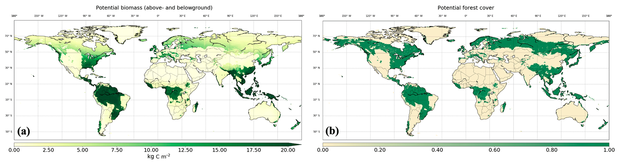
Figure 1 Potential biomass density (a) and potential forest cover (b) in 850 estimated by GLM2 model.

Standardization of LULCC data is critical for CMIP6 to simplify intercomparison of the ESMs and facilitate model analysis. The CMIP6 requires the LUH2 as standard land-use input for all ESMs; however, the data standardization could be undermined if models implement the LUH2 differently, such as applying different rules to translate the LUH2 into land-cover change, which is essential for models. Identifying the consistent rules between models for the LUH2 use is critical for two reasons. First, although land-use changes are generally associated with a change in land cover and carbon stocks (see Fig. 1 in Pongratz et al., 2018), these two changes are not always equivalent, and the degree of land-cover alteration varies with the types of land-use changes and the location where land-use changes happen. An inconsistent land-cover translation from the same land-use products will potentially produce variance in land-cover dynamics across models and in turn impact the land surface biophysical and biochemical processes. Second, the HYDE 3.2 data underlying LUH2 has redefined the former pasture category used in CMIP5 into the two subcategories of “managed pasture” and “rangeland” (with the total being termed “grazing land”). This redefinition intends to mitigate the pasture anomaly by suggesting different treatments of vegetation and carbon removal in models for these two types of land-use changes (Klein Goldewijk et al., 2017). However, explicit suggestions are not yet provided for land cover resulting from these newly defined land-use types. Therefore, a consistent rule across models for the LUH2 translation is needed, with potential to reduce impacts of inconsistent LUH2 usage on studying land-use effects through CMIP6.

To recommend a rule for translating historical land-use changes from the LUH2 for CMIP6 models, this study investigates the impacts of land-use change on land cover by proposing several alternative sets of translation rules, which are then integrated into the Global Land-use Model 2 (GLM2) (Hurtt et al., 2019, 2020) to simulate the forest cover and carbon dynamics. These simulations are then evaluated against estimates of contemporary forest cover and carbon density from remote sensing observations, and the resulting cumulative LULCC carbon emissions are compared with a range of independent estimates.

2 Methodology

In this study, two key land-cover properties (i.e., forest cover and vegetation carbon) are simulated by combining historical land-use change with translation rules. The historical land-use change information is specified by the LUH2 dataset (v2h, available at https://doi.org/10.22033/ESGF/input4MIPs.10454),which serves as the forcing data for a new generation of advanced ESMs as part of CMIP6. Section 2.1 describes the details of land-use change characterization, and Sect. 2.2 defines each translation rule. The resulting forest cover and vegetation carbon is tracked in each grid cell (${\mathrm{0.25}}^{\circ }\times {\mathrm{0.25}}^{\circ }$) for the years 850 to 2015 using methods described in Sect. 2.3 and 2.4. The simulated forest cover and vegetation carbon are then compared with multiple published datasets of land-cover, carbon stock and estimates of land-use change emissions (see details in Sect. 2.5).

2.1 Land-use change characterization

The LUH2 dataset was generated with the GLM2 (Hurtt et al., 2019, 2020), which, like its predecessors (Hurtt et al., 2006, 2011), estimates annual sub-grid-cell land-use states and transitions by including multiple constraints such as gridded patterns of historical land use from the HYDE database (Klein Goldewijk et al., 2017), historical national wood harvest reconstructions, potential biomass and recovery rates, and others. Building upon previous work from CMIP5, for which the original LUH1 dataset was used, the LUH2 has extended the time span to 850–2100 and increased spatial resolution to ${\mathrm{0.25}}^{\circ }\times {\mathrm{0.25}}^{\circ }$. In addition, the LUH2 includes 12 different land-use types (i.e., forested and non-forested primary and secondary land, cropland of C3 annual, C3 perennial, C4 annual, C4 perennial and C3 nitrogen-fixing, urban, managed pasture, and rangeland) and includes transitions between all combinations of these categories.

In the LUH2, “primary” refers to land previously undisturbed by any human activities since 850, while “secondary” refers to land undergoing a transition or recovering from previous human activities. Global secondary land area was specified as zero in 850. Note that primary and secondary lands are further subdivided into forested and non-forested grids using a definition based on the potential aboveground biomass density (forested land requiring an aboveground biomass density ≥ 2 kg C m⁻²).

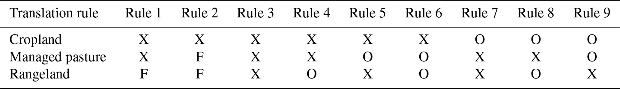
Table 1 Rules for vegetation clearance during cropland, pasture and rangeland expansion. “X” indicates complete removal of vegetation if the primary and secondary land state is altered. “O” indicates no vegetation removal when land-use change occurs. “F” indicates that vegetation is only removed if the preceding land cover is forested primary or forested secondary land.

2.2 Translation rules

Nine translation rules are proposed (Table 1) to analyze the effects of land-use change on land-cover dynamics, whereby each rule differs in treatment of vegetation cover and vegetation carbon stock during land-use changes. Rules 1–4 all assume complete clearance of vegetation for cropland and vary on vegetation clearance for managed pasture and rangeland. Rules 5–9 are added for analytical purposes, rather than as realistic possibilities. For example, Rule 3 presumes all land-use changes alter land cover and reduce carbon stock, and this rule would produce the least global forest cover and carbon stock. Rules 1 and 3 differ in treatment of vegetation in non-forested land when converted to rangeland, and the resulting difference between their carbon stocks indicate the impact of rangeland expansion on non-forests and also tests whether the disaggregation of grazing land into managed pasture and rangeland will address the pasture anomaly issue in 1950–1960. Rule 1 (clearance of all vegetation for cropland and managed pasture; and only forest clearance for rangeland) is in fact the rule suggested in the underlying HYDE dataset and its distinction between pasture and rangeland (Klein Goldewijk et al., 2017). For simplicity, we do not consider partial removal of vegetation in this study; vegetation is either fully removed or fully remains as these land-cover transitions represent the maximum and minimum bounds for land-cover alteration. In this study, the translation rules are applied to all regions and are constant across the whole simulation period. Although the impacts of land-use change on land cover may vary in different regions, the discussion of region-varied and time-varied translation rules is beyond the scope of this study.

It is important to note that these nine rules are not equally realistic, and the purpose of including Rules 5–9 is to investigate individual or joint contributions of cropland, managed pasture and rangeland expansion on forest and carbon. For example, forest and carbon dynamics resulting from Rule 6 could suggest the individual impact of cropland expansion.

2.3 Simulation of land-cover change

In this study, land-cover change is simulated by performing a modified GLM2 simulation in which the computed land-use transition rates (using the same methodology as LUH2) are supplemented with a set of translation rules (Table 1) to track forest cover change and carbon dynamics at 0.25^∘ spatial resolution. Note that the modified GLM2 still generates and tracks the exact same land-use transitions of the LUH2 and has additional functions to track associated land-cover change in terms of forest cover and vegetation carbon. GLM2 uses a statistical model to estimate ecosystem stocks and fluxes with temperature and precipitation as inputs (see Hurtt et al., 2002, for details). The annual temperature and precipitation maps from MSTMIP (Wei et al., 2014) were averaged over 1901 and 2000 to generate the spatially varied and temporally static climatological temperature and precipitation, which was then used to spin up the GLM2 globally at ${\mathrm{0.25}}^{\circ }\times \mathrm{0}$. 25^∘ resolution for 500 years. The climatology stays as constant over the spinup period, and other environmental factors were not taken into consideration such as CO₂ fertilization, nitrogen limitation and climate variability.

When land is converted to cropland, managed pasture and/or rangeland, each translation rule indicates that vegetation in primary and secondary may be cleared or remain intact as the result of land-use changes. For example, for a given land-use transition rate from forest to managed pasture, if the applied translation rule indicates the clearing of the vegetation completely, then the resulting grid cell vegetation fraction in the forest land-use type is reduced equal to the amount of pasture gained. If the rule indicates not to clear vegetation, then only the land-use type will be changed to pasture, and the vegetation area will be unchanged, but the vegetation will be influenced by the management in terms of stand age/biomass, which are assumed to cease growing due to pressure from subsequent human management. If this pasture land is further converted to other non-primary and non-secondary land (e.g., cropland, rangeland or urban), the vegetation remaining from previous forest–pasture conversion then will be totally cleared. Therefore, the vegetation fraction existing within the cropland, managed pasture, rangeland and urban of each grid cell can be tracked via the following equation:

$$\begin{array}{}\text{(1)}& \begin{array}{rl}& f(i,t+\mathrm{1})=fi,t)+f^{\text{gained}}(i,t)-f^{\text{lost}}(i,t)\\ & (i=\mathrm{5},\mathrm{6},\mathrm{7},\mathrm{8}),\end{array}\end{array}$$

where f(i,t) is the fraction of grid cell that is vegetated in land-use type i (i.e., classes 5–8: cropland, managed pasture, rangeland and urban) at time t; f^gained(i,t) and f^lost(i,t) are gained and lost vegetation fractions, respectively. The vegetation fraction could only be gained in land-use change from primary and secondary land (both forested and non-forested) and be lost in land-use change to any other land-use types except forested and non-forested primary land.

$$\begin{array}{}\text{(2)}& \begin{array}{rl}& f^{\text{gained}}(i,t)={\sum }_{j=\mathrm{1}}^{\mathrm{4}}{a}_{ij}(\mathrm{1}-{\mathit{\gamma }}_{ij})\\ & (i=\mathrm{5},\mathrm{6},\mathrm{7},\mathrm{8};j=\mathrm{1},\mathrm{2},\mathrm{3},\mathrm{4})\end{array}\end{array}$$

$$\begin{array}{}\text{(3)}& \begin{array}{rl}& f^{\text{lost}}(i,t)={\displaystyle \frac{f\left(i,t\right)}{l\left(i,t\right)}}{\sum }_{k=\mathrm{1},k\ne i}^{\mathrm{8}}{a}_{ki}\\ & (i=\mathrm{5},\mathrm{6},\mathrm{7},\mathrm{8};k=\mathrm{3},\mathrm{4},\mathrm{\dots },\mathrm{8})\end{array}\end{array}$$

The possible values of i, j and k are 1, 2, …, 8, representing primary forested land, primary non-forested land, secondary forested land, secondary non-forested land, cropland, managed pasture, rangeland and urban, respectively. a_ij is the land-use transition fraction estimate by the LUH2 from land-use type j (i.e., primary forested land, primary non-forested land, secondary forested land and secondary non-forested land) to land-use type i; γ_ij represents the translator factor to convert land-use change to land-cover change, it equals 1 if the translation rule in Table 1 indicates an “X” or “F” for this land-use change. For example, γ_ij is 1 for land-use change from primary land (forested, non-forested grids) to cropland in Rules 1 and 2 but 0 for the same type of change in Rules 8 and 9. This translator factor is 1 for all types of land-use change in Rule 3 since all vegetation is cleared during all land-use changes. l(i,t) is the land-use fraction estimate by the LUH2 for type i at time t, and this fraction is larger than or equal to its vegetation fraction f(i,t).

Vegetation in primary and secondary land can remain or be lost in land-use changes to cropland, pasture or rangeland depending on translation rules. According to the definition of primary land in the LUH2, its transition to other land-use types is unidirectional; thus primary land could not gain vegetation from any land-use changes. Wood harvest on primary land will result in vegetation loss and a change in land-use type to secondary land, but harvest on secondary land will not change the land-use type. Furthermore, vegetation in secondary land could be gained from harvest on primary land and may be gained through the process of abandonment of cropland, pasture or rangeland depending on translation rules. Note that reforestation but not afforestation is also considered in this study. The former is to re-establish forest on the land which has been forested before, while the latter is an anthropogenic activity to establish forests on land which has never been forested. Thus, the vegetation of primary and secondary land is tracked by the following equation:

$$\begin{array}{}\text{(4)}& \begin{array}{rl}& f(i,t+\mathrm{1})=f(i,t)-f^{\text{lost}}(i,t)+f^{\text{gained}}(i,t)\\ & (i=\mathrm{1},\mathrm{2},\mathrm{3},\mathrm{4}),\end{array}\end{array}$$

$$\begin{array}{}\text{(5)}& f^{\text{lost}}(i,t)=\left\{\begin{array}{ll}{\sum }_{j=\mathrm{5}}^{\mathrm{8}}{a}_{ji}+b_i,& (i=\mathrm{1},\mathrm{2};j=\mathrm{5},\mathrm{6},\mathrm{7},\mathrm{8})\\ {\sum }_{j=\mathrm{5}}^{\mathrm{8}}{a}_{ji}{\mathit{\gamma }}_{ji},& (i=\mathrm{3},\mathrm{4};j=\mathrm{5},\mathrm{6},\mathrm{7},\mathrm{8}),\end{array}\right.\end{array}$$

$$\begin{array}{}\text{(6)}& \begin{array}{rl}& f^{\text{gained}}(i,t)={\sum }_{k=\mathrm{5}}^{\mathrm{8}}{\displaystyle \frac{f(k,t)}{l(k,t)}}{a}_{ik}+b_j\\ & (i=\mathrm{3},\mathrm{4};j=\mathrm{1},\mathrm{2};k=\mathrm{5},\mathrm{6},\mathrm{7},\mathrm{8}),\end{array}\end{array}$$

where f(i,t) is fraction of vegetation at land-use category i (primary forested land, primary non-forested land, secondary forested land, secondary non-forested land) at time t. a_ji is the land-use transition fraction from primary and secondary land to cropland, managed pasture, rangeland and urban in the LUH2. b_i or b_j is the wood harvest fraction from primary or secondary (forested or non-forested) land. f(k,t) and l(k,t) are the vegetation fraction and land-use fraction in land-use type k (i.e., cropland, managed pasture, rangeland and urban), and a_ik is the land-use transition due to land-use abandonment.

2.4 Simulation of vegetation carbon dynamics

Vegetation carbon stocks fluctuate through releasing and accumulating carbon in response to natural growing conditions, disturbances and anthropogenic land-use changes, which can vary widely in terms of their carbon impacts. For land-use changes associated with clearing or harvesting vegetation, the forest biomass is either released immediately (e.g., burning) or stored in soil pools or as timber products (both of which eventually decay over decades). However, when managed land is abandoned and allowed to recover, the vegetation takes up CO₂ from the atmosphere through photosynthesis, resulting in increasing carbon stocks in vegetation and possibly soils. The magnitude of each of these bidirectional carbon flows ultimately determine if the land is a net carbon sink or carbon source. In this study, the temporal dynamics of carbon fluxes after land-use change are simplified, with all biomass (above- and belowground) being released instantaneously to the atmosphere. Note that the biomass stock change is a rough proxy of actual net land-use change fluxes, for which delayed emissions from litter and soil carbon and product pools needed to be accounted for as well as instantaneous emissions from burning biomass. Changes in soil carbon associated with loss of vegetation biomass are usually associated with carbon losses but are likely less important than biomass changes, as are net fluxes from product pool changes (Erb et al., 2018).

Similar to the land-cover change simulation in Sect. 2.3, if translation rules indicate vegetation clearing at the expansion of cropland, managed pasture, rangeland or urban land, vegetation biomass is totally released as a carbon emission, and its age is set as zero. If vegetation is not cleared based on translation rules, the biomass remains but ceases to increase, and the age of this vegetation also remains unaffected, because the age is used in this model only for the calculation of biomass density. Keeping age fixed corresponds to keeping biomass from further growing, which represents the influences of management. If the land is abandoned and converted back to secondary land, a mean age is calculated over all vegetation with different ages, then the mean age increases year by year, and biomass regrows towards equilibrium. Thus, the biomass density in secondary vegetation at time t is calculated for each grid cell using its mean age, potential biomass and potential NPP:

$$\begin{array}{}\text{(7)}& B\left(t\right)=B_{\mathrm{0}}\left(\mathrm{1}-e^{-{\text{NPP}}_{\mathrm{0}}\times G\left(t\right)/B_{\mathrm{0}}}\right),\end{array}$$

where B(t) is the aboveground biomass density of vegetation in secondary land at time t, B₀ is the potential aboveground biomass density from the GLM2 model and varied by grid location, NPP₀ is the potential NPP of the wood fraction that is allocated to cumulate stem and branch biomass annually, and G(t) is the mean age of secondary vegetation. Note that B₀ and NPP₀ are estimated by a statistical model in GLM2 using climatological temperature and precipitation and are spatially varied but temporally constant over the simulation period of 850 to 2015. Above- to belowground biomass ratio is assumed as 3 : 1 when converting aboveground biomass to total biomass (above- and belowground), and biomass density is converted to carbon by a ratio of 0.5.

Table 2 Summary of land cover products used in this study including six satellite-based datasets and FAO FRA report.

Plants cultivated by human management (e.g., crops and orchards) are not tracked in this study; zero biomass is assigned to cropland, managed pasture, rangeland and urban use types. However, carbon is tracked for vegetation remaining from primary or secondary due to the translation rules, as well as lands that convert from human management back to natural lands. Thus, the total carbon stocks in this study are expected to be lower than other estimates (Houghton, 2003; Saatchi et al., 2011), especially in the grids with a higher fraction of non-primary and non-secondary land use.

2.5 Diagnostics for evaluating translation rules

To evaluate which translation rules best translate land-use changes to land-cover changes, the simulation results were compared with contemporary forest cover and carbon density maps from remote sensing observations and other estimates, as well as LULCC carbon emissions from other studies using different models. Contemporary values of forest cover and carbon density are used for two reasons. First is the lack of multiple diagnostics of forest cover and carbon density across the whole simulation period (i.e., 850 to 2015). Second is that contemporary values could potentially reflect cumulative error in converting land-use change to land-cover change since 850. We assume that if a translation rule produces a best match with the diagnostic maps of forest cover and carbon density, then it would also produce the best estimate for the historical period.

Diagnostics of contemporary forest cover consist of six widely used satellite-based land-cover and tree coverage datasets (Bartholomé and Belward, 2005; Bicheron et al., 2008; DeFries et al., 2000; Friedl et al., 2010; Hansen et al., 2013; Loveland et al., 2000) (see Table 2) and the Global Forest Resources Assessment (FRA) 2015 (FAO, 2015). In Table 2, GLCC, GLC2000, GlobCover and MODIS LC are land-cover datasets rather than tree cover and were produced based on different classification schemes resulting in different land-cover legends. Prior to being used as diagnostics in this study, they needed further reclassification of their land-cover legends into a common representation of forest canopy cover at the same spatial resolution (0.25^∘) by the following procedures. First, the GLCC, GLC2000, GlobCover and MODIS LC were converted to tree cover fraction based on Table S1 at their native resolutions (Song et al., 2014). Then, all six datasets were resampled to 1 km resolution and translated to a binary (forest versus non-forest) map by applying a 30 % tree-cover threshold (Sexton et al., 2016). Through counting the percentage of pixels marked as forest within each ${\mathrm{0.25}}^{\circ }\times {\mathrm{0.25}}^{\circ }$ grid cell, six global gridded forest cover maps at 0.25^∘ spatial resolution were generated, and resulting global forest areas of each dataset are shown in Table 2. As these satellite-based datasets were developed from different sensors (e.g., AVHRR, SPOT-4, MERIS, MODIS and Landsat) and models (regression trees, decision tree, clustering labels and random forests), an averaged map (hereinafter referred to as “averaged satellite-based forest cover”) was generated to accompany the six forest cover maps to examine the spatial pattern of contemporary forest cover simulated by each translation rule. In addition, since FAO only reports national forest cover (not spatially explicit), these data were only used for comparison at the country level.

Table 3 Summary of carbon emissions due to LULCC from available studies in the preindustrial and industrial periods.

Carbon density maps are employed as the second metric to evaluate the translation rules. Two datasets were employed: the IPCC Tier-1 biomass carbon map for the year 2000 (Ruesch and Gibbs, 2008) and a pantropical biomass map (hereinafter referred to as Baccini's product; Baccini et al., 2012). The former, a global above- and belowground carbon density map, is created by dividing the globe into 124 carbon zones by land cover, continental regions, eco-floristic zones and forest age and assigning each zone a unique carbon stock value. The latter is estimated by combining ground plots, GLAS lidar observations and optical reflectance of MODIS. This dataset employs the empirical relationship between aboveground biomass and tree diameter at breast height and estimates aboveground biomass density for pantropical regions (40^∘ S–30^∘ N). Both carbon density maps were resampled to 0.25^∘ before evaluation.

In addition, the ability of the translation rules to reproduce LULCC carbon emissions is also assessed. The estimates of LULCC carbon emissions were compiled from published papers (Table 3) (Houghton, 2010; Houghton and Nassikas, 2017; Le Quéré et al., 2018; Pongratz et al., 2009; Reick et al., 2010; Shevliakova et al., 2009; Stocker et al., 2011). These studies have significant discrepancy in emissions estimates as they employed various methods (e.g., bookkeeping methods and different process-based models) and LULCC datasets and considered different types of land-use change activities. They also differ in the treatment of environmental change (for example, Pongratz et al., 2009; Reick et al., 2010; Shevliakova et al., 2009; Stocker et al., 2011, include effects of evolving climate or atmospheric CO₂ concentration on LULCC emissions, which is not accounted for in bookkeeping model-based studies, Houghton, 2010; Houghton and Nassikas, 2017). In this study, only the range of these estimates during the preindustrial and industrial periods are chosen to evaluate the translation rules. We posit that the recommended translation rule should not produce anomalous carbon emissions that are outside the compiled range.

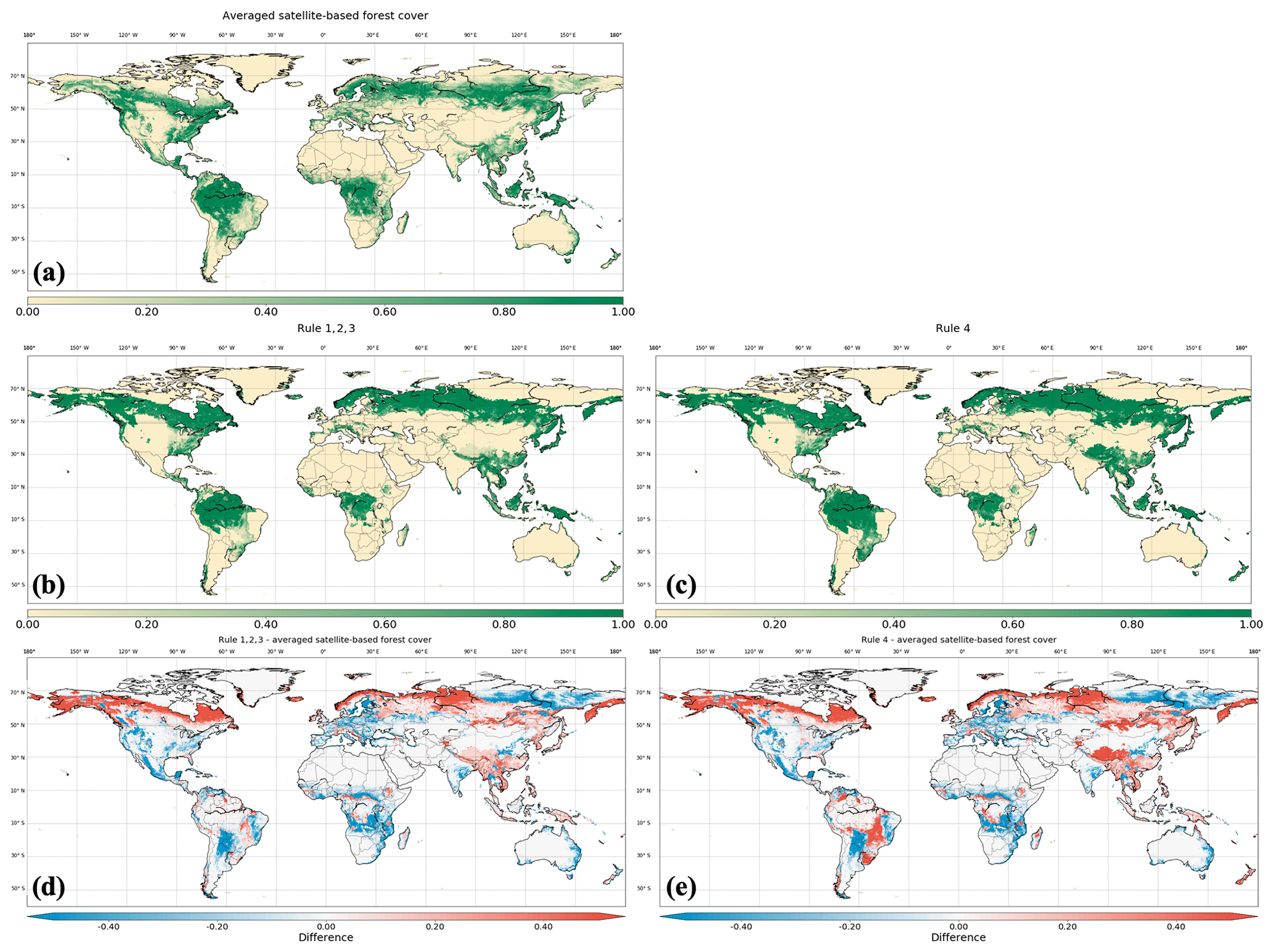
Figure 2 Forest cover in 2000 from the averaged satellite-based forest cover in (a); Rule 1, 2, 3 in (b); and Rule 4 in (c). Panels (d) and (e) are maps of forest cover difference between (b) and (a) and (c) and (a), respectively.

In summary, the GLM2-based estimates of forest cover and carbon density in the year 2000 and LULCC carbon emissions during the periods 850–1850 and 1850–2000, based on nine different translation rules are compared with the above three types of diagnostics (i.e., contemporary forest cover/area and carbon density maps and LULCC emissions). The final recommended translation rules should produce (1) the forest cover with the smallest difference with diagnostic maps at global, country and grid scale; the total forest cover at global and country level should be comparable to the range of diagnostics, and spatial pattern should also be close to diagnostics; (2) the closest carbon density map compared to diagnostics with the smallest difference, comparable spatial pattern and total carbon stock as well; and (3) reasonable LULCC carbon emissions within the range from other diagnostic estimates and minimizing the anomalous emissions during 1950–1960.

3 Results

3.1 Potential forest cover and biomass carbon

The GLM2 estimates global vegetation carbon stock (including above- and belowground) in 850 as 718 Pg C, and the resulting potential biomass map is shown in Fig. 1a. For comparison, global potential vegetation carbon stock was estimated as 557 Pg C in Kucharik et al. (2000), 772 Pg C in Pan et al. (2013) and 923 Pg  C in Sitch et al. (2003). Forested land in GLM2 is defined as land which has aboveground potential biomass of at least 2 kg C m⁻² (Hurtt et al., 2006, 2011). With this definition, global potential forest area was estimated as 47.82×10⁶ km², and the resulting potential forest cover map is shown in Fig. 1b. For comparison, global potential forest area was estimated as 48.68×10⁶ km² in Pongratz et al. (2008), and potential forest and woodland area was 55.3×10⁶ km² in Ramankutty and Foley (1999).

3.2 Forest cover evaluation

The global gridded forest cover maps resulting from Rules 1–9 in 2000 are generally consistent in forest extent with satellite-based observations (shown in Figs. 2 and S6 in the Supplement). For example, they all estimate high forest cover in tropical rainforests and northern boreal forests but low cover in the western USA, eastern Europe and Central Asia. As Rules 1, 2 and 3 only differ in whether to clear vegetation and carbon in the conversion from non-forest to managed pasture or rangeland, the forest cover resulting from Rules 1, 2 and 3 are the same. All of the rules (1–9) consistently estimate higher forest cover than the averaged satellite-based forest cover in West Siberia and southern China and lower forest cover in African savannas and East Siberia, western Mexico, and Argentina. Separately, Rules 4, 6, 7, 8 and 9 show larger forest cover than Rules 1, 2, 3 and 5 in the south and southeast of Brazil and Tibet in China.

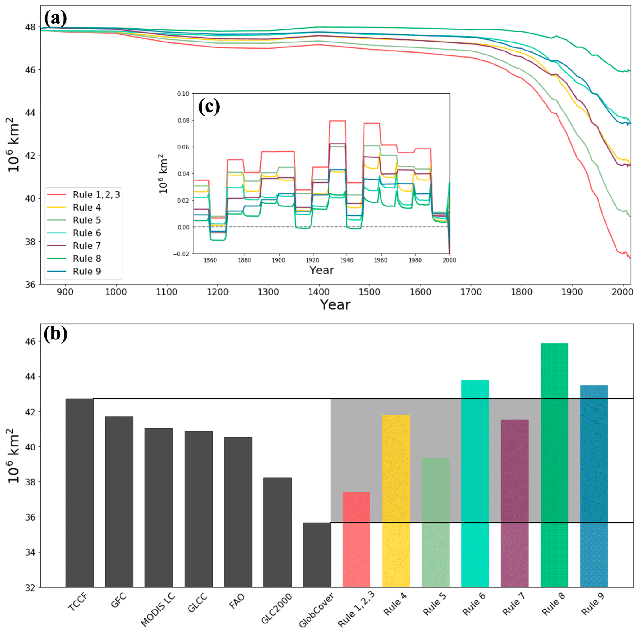
Figure 3 (a) Global forest area resulting from translation rules from 850 to 2015; (b) comparison of global forest area in 2000 between remote sensing and FAO (shown as black bars) and results of translation rules (colored bars); (c) annual change rate from 1850 to 2000. Positive values indicate forest loss.

The total area of global forest in 850 amounts to 47.82×10⁶ km² according to the GLM2 model (Fig. 1b and. 3a) when all forested lands were in a primary state by definition and decreased thereafter (Fig. 3a). Forest loss has accelerated since the beginning of the Industrial Revolution and shows relatively high annual change rates (shown in Fig. 3c). The translation rules produce a wide range of global forest cover in 2000 from 37.42 to 45.89×10⁶ km². In Rules 1, 2, and 3, the global forest is lost at the highest rate due to all land-use change activities on forested land resulting in the clearing of forest, and only 37.42×10⁶ km² of global forest is left in 2000 under these three rules. In contrast, under Rule 4 forest remains during rangeland expansion, and this would result in greater forest cover (e.g., 41.80×10⁶ km² in 2000; Table 4). The forest losses in Rules 6, 8 and 9 indicate the individual contribution of cropland, managed pasture and rangeland expansion. For example, rangeland and cropland expansion results in the most and second most of forest loss with an area of 4.34 and 4.06×10⁶ km², respectively, during 850–2000.

Six satellite-based forest cover datasets and FAO data report the global forest area around the year 2000 ranging from 35.66 to 42.74×10⁶ km². One of the major reasons underlying the discrepancy in global forest area is the difference in defining “forest”, particularly in the regions with intermediate tree cover (Sexton et al., 2016). The global forest area in the year 2000 resulting from the translation rules are compared to the range of seven diagnostic estimates (Fig. 3b). The forest cover based on Rules 6, 8 and 9 is beyond the range of the diagnostics, indicating that these rules underestimate the impacts of land-use change on land cover and overestimate the global forest existing in the present day. The excessive remaining forest cover in these three rules also rejects these rules' assumptions that only a particular type of land-use change would alter the land cover. In contrast, Rules 1–4, 5 and 7 produced estimates of global forest area within the range of diagnostics.

Table 4 Forest area (10⁶ km²) in 2000 of eight countries with the largest forest area and all other countries combined (“Others”), estimated by the nine translation rules, range compiled from satellite-based datasets and FAO report.

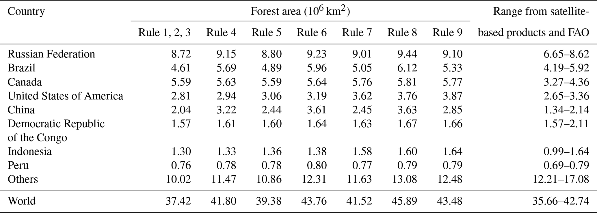
The forest cover estimation from translation rules are further compared with diagnostic datasets at the country level (Table 4). In the diagnostic forest cover datasets, three-fourths of global forest cover lies within eight countries: the Russian Federation, Brazil, Canada, United of States of America, China, the Democratic Republic of the Congo, Indonesia and Peru. The forest cover estimates from Rules 1–4 are generally well within the range of diagnostics. For example, six of eight countries have estimates within the range for Rules 1, 2 and 3 and five of eight countries for Rule 4. China and Brazil are the two countries where Rules 1–3 and Rule 4 have a relatively larger difference between their estimates; the difference between Rules 1, 2 and 3 and Rule 4 are 1.17 and 1.08×10⁶ km² for China and Brazil, respectively. Rules 5 and 7 overestimated the forest area of China, the Russian Federation and Canada though their global forest areas are within the range of the diagnostic and are within range for Brazil, the Democratic Republic of the Congo, Indonesia and Peru.

These comparisons evaluate the resulting gross forest cover of the translation rules at global and country levels. Further examination at the grid level is also needed. Since the FAO report only provides national forest cover, the averaged satellite-based forest cover map and each of the six satellite-based forest cover maps were used to calculate the average of the absolute differences across global grids (Fig. 4). Rules 1, 2 and and 3 consistently produce the smallest overall difference compared to Rule 4 and other rules regardless of which satellite-based forest cover is chosen as the reference. The average absolute difference (AAD) of Rule 1, 2, 3 is under 90 km² compared to the averaged satellite-based forest cover map and even smaller compared to the GFC. The smallest difference of all rules across six reference forest maps indicates that the GLC2 may have a more similar spatial distribution to the GFC estimate. Regional comparison of average of absolute difference (Fig. S1) suggests Rules 1, 2 and 3 give a better estimate of forest cover at the north and south temperate zones (i.e., 60–23^∘ N and 23–60^∘ S) than tropical zones (23^∘ N–23^∘ S). All rules have similar AAD at the 60–90^∘ N zone.

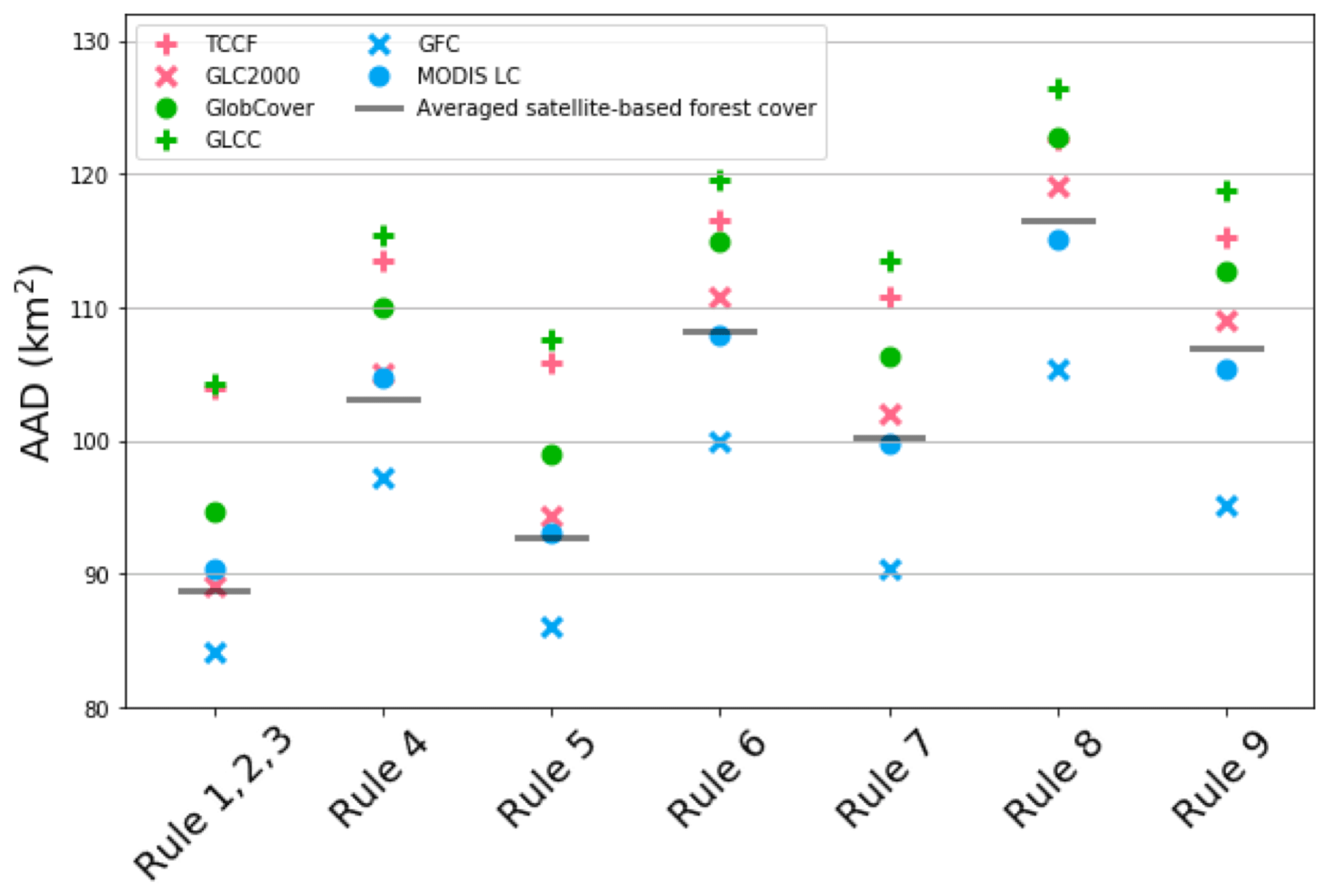
Figure 4 Global average of absolute difference in forest area between maps estimated by translation rules and each of the six satellite-based forest cover maps as well as the averaged satellite-based forest cover map.

3.3 Evaluation of carbon dynamics

The net carbon emissions of the nine translation rules were calculated over two periods (850 to 1850 and 1850 to 2000) and compared to other studies (Table 5). Rules 1–4 produced similar patterns to other studies, specifically that global carbon emissions of 1850–2000 are twice as large as that of 850–1850. However, the emissions estimates of each period varied among Rules 1–4, from 55 to 77 Pg C during 850–1850 and from 142 to 185 Pg C during 1850–2000, due to the assumptions for clearing vegetation during land-use change. For example, Rule 3 produced the largest emissions as the carbon in both forested and non-forested land is released for all land-use changes, and Rule 1 produces fewer emissions since the vegetation is not cleared and carbon is not released when non-forested land is converted to rangeland. In general, Rules 1, 2, 3 and 4 estimated comparable emissions with other studies, while the emissions of the Rules 6–9 are out of range (Table 5).

Table 5 Summary of LULCC carbon emissions estimated by the nine translation rules and those from other studies in Table 3.

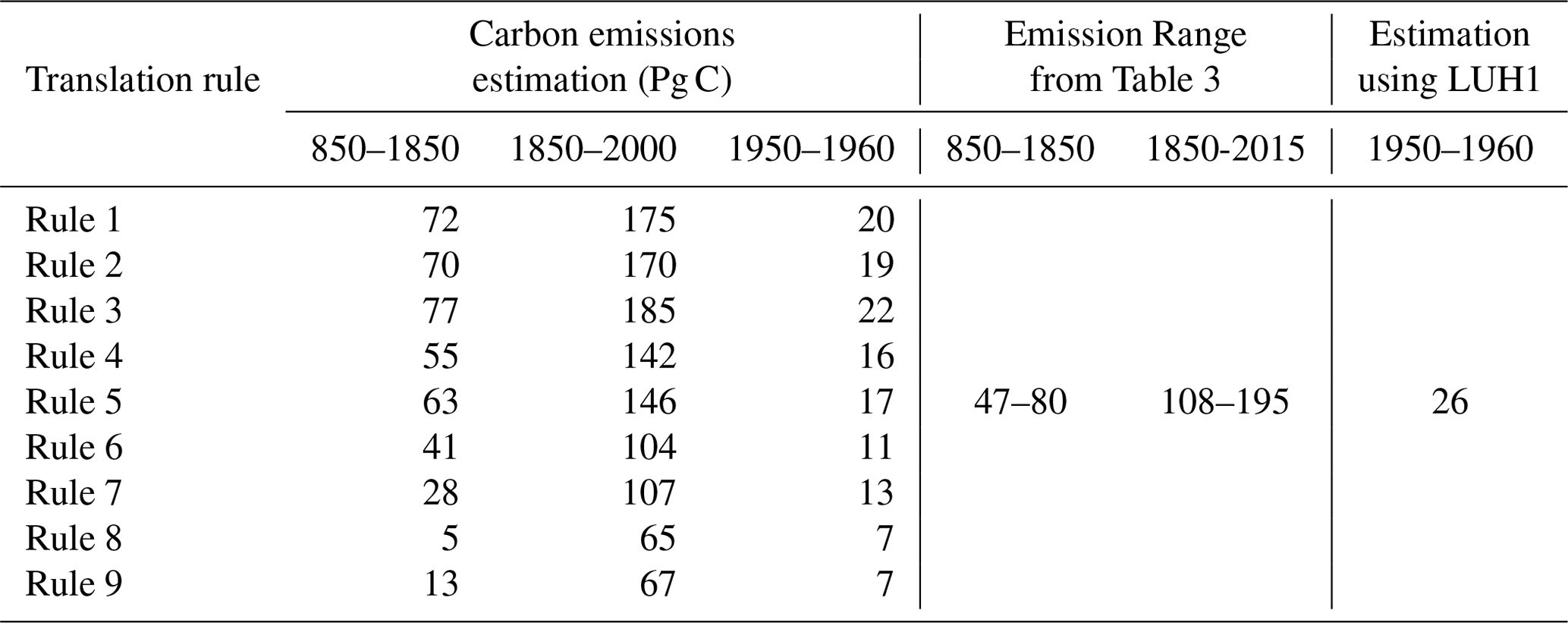
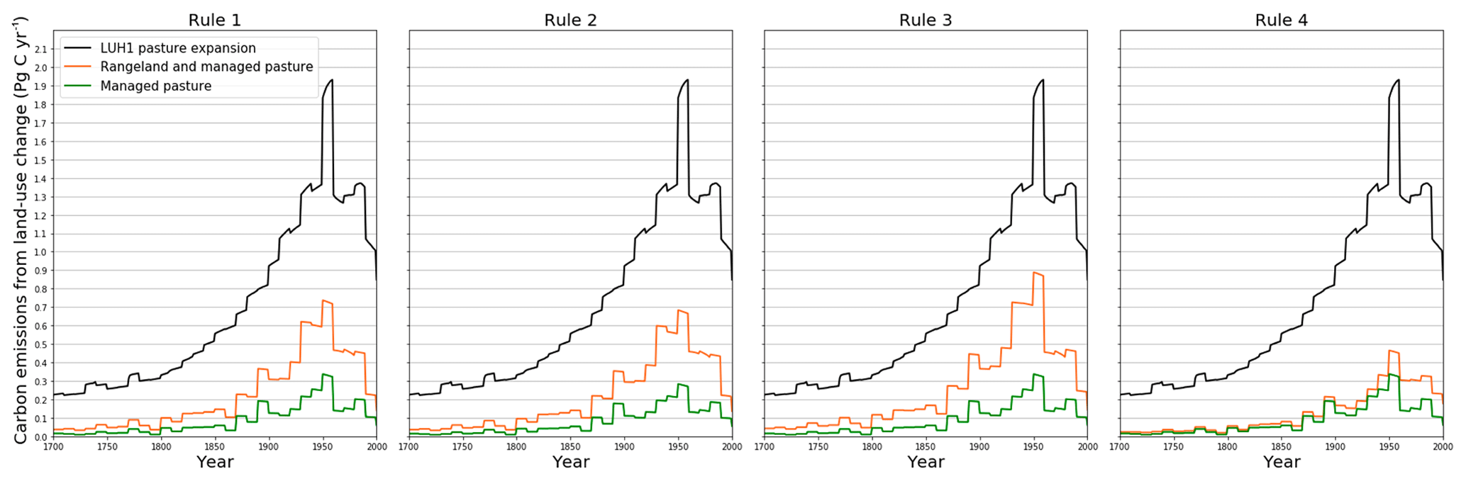
Figure 5 Carbon emissions due to vegetation (forest and non-forest) removal in expansion of managed pasture and rangeland. Black line represents emissions from pasture expansion in LUH1. Orange and green lines represent emissions from expansion of managed pasture and rangeland and from expansion of just managed pasture, respectively, in LUH2. Note that the pasture category in LUH1 corresponds to managed pasture and rangeland together in LUH2.

Carbon emissions from pasture expansion were calculated for LUH1 (Hurtt et al., 2011), and this is used as a baseline to assess the improvement of translation rules on the pasture anomaly. Rules 1–4 estimate fewer emissions during this decade and decrease the anomaly between 4 and 10 Pg C. Rule 1 reduces anomalous emissions by 6 Pg C, indicating the sole contribution of the LUH2 to mitigating pasture anomaly. In LUH1, the anomalous emissions spike during 1950–1960 mainly arises from overestimating the emissions from pasture expansion, especially in three regions (i.e., Africa, East, South and Central Asia, and North America). The carbon flux from expansion of managed pasture and rangeland in the LUH2 was reduced at global (Fig. 5) and regional (Fig. 6) scales in simulations based on Rules 1, 2 and 3. Note that the pasture land in LUH1 corresponds to rangeland and managed pasture together in the LUH2. Rule 2 reduces more anomalous emissions than Rule 1 (reduced 6 Pg C in Rule 1 and 7 Pg C in Rule 2), because Rule 1 completely clears vegetation when transitioning to managed pasture, whereas Rule 2 only removes vegetation if the preceding land cover is primary or secondary forest.

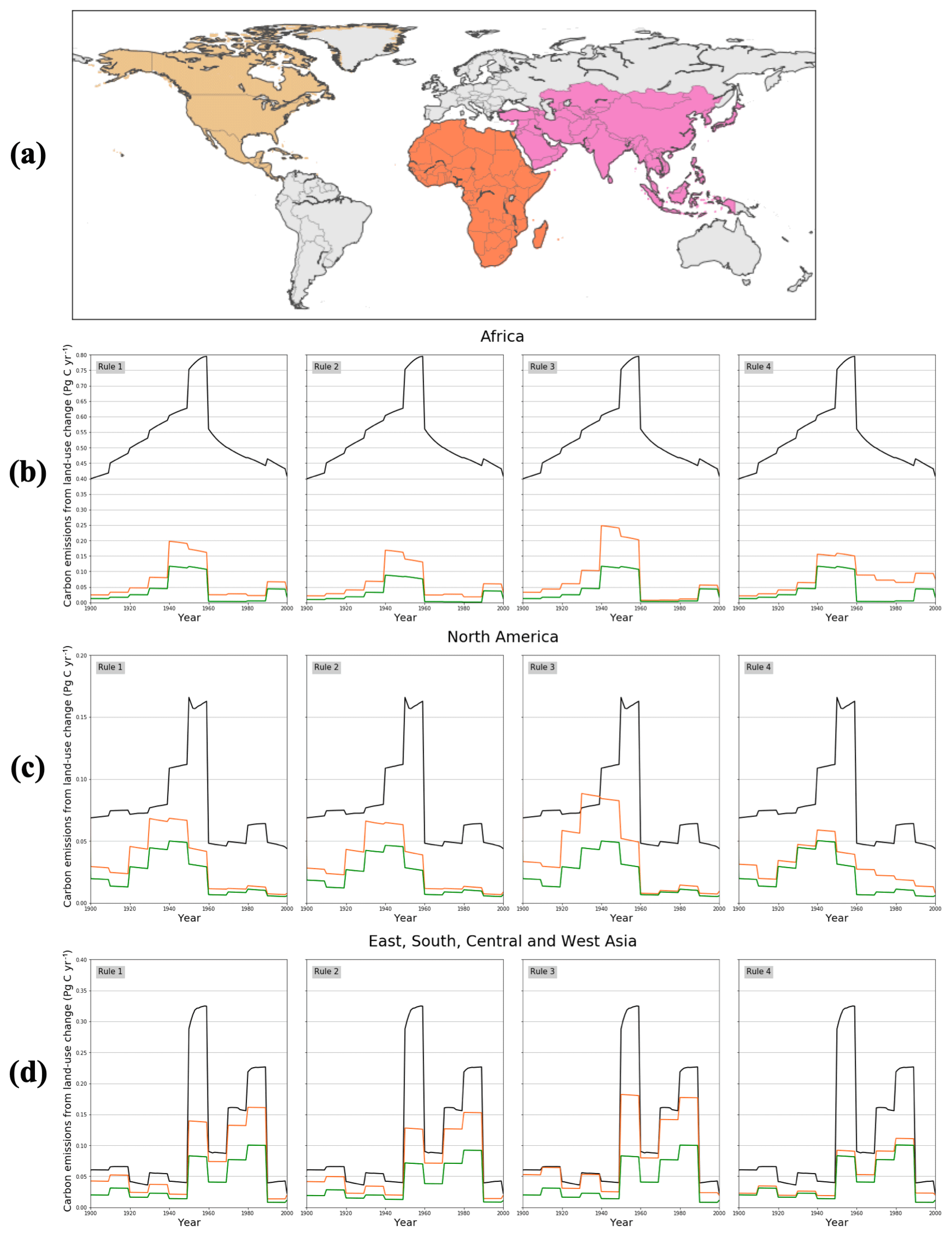
Figure 6 As in Fig. 5 but three regions: (b) Africa; (c) North America; and (d) East, South, Central, and West Asia. Panel (a) illustrates the defined boundaries of (b)–(d).

Figure 7 (a) IPCC Tier-1 biomass density; (b) Baccini's product (only aboveground) at pantropical; global carbon density (above- and belowground) maps estimated by Rules 1–4 from (c) to (f).

Rules 1–4 generally capture the spatial pattern that carbon density in tropical rainforest regions is much higher than northern boreal forests (Fig. 7). These four rules overestimate carbon density at high latitudes of the Northern Hemisphere, in South China and in the Amazon rainforests but underestimate density across much of sub-Saharan Africa, Mexico and the southwestern part of the United States (Figs. S2 and S3). To further examine the spatial pattern of estimated carbon density, the estimates from all rules were compared to the carbon density maps of IPCC Tier-1 (above- and belowground) globally and Baccini's dataset (only aboveground) at the pantropical scale by calculating averaged absolute difference (Fig. 8). According to this comparison, Rules 1–3 best capture the carbon density globally (Fig. 8). Regional comparison of the IPCC Tier-1 biomass map and rule estimates indicate Rules 1–4 have comparable AADs of carbon density at the zone of 90–60^∘ N; the AAD difference between four rules is largest at 23–60^∘ S, followed by 23–23^∘ S and 23–60^∘ N (Fig. S4). Carbon density estimates of Rules 1–3 were further examined in regions where their estimates have a difference (shown in Fig. S5a). The spatial pattern (Fig. S5c–f) and histogram (Fig. S5b) of carbon density differences between rules and IPCC Tier-1 biomass estimates show that all three of these rules underestimate carbon density, and more grids are less underestimated in Rules 1 and 2 than Rule 3. The underestimation is expected because biomass of human cultivated vegetation is not tracked, nor is growth of natural vegetation on cropland and pasture and rangeland. However, uncertainty levels of the IPCC Tier-1 biomass should be taken into account when determining rule performance. Three bias levels of IPCC Tier-1 biomass map (i.e., ±10 %, ±20 % and ±30 %) were considered (Fig. S5b). At these levels of uncertainty in the reference, Rules 1–3 could not be distinguished in performance. Finally, the carbon stock comparison between Rules 1–3 (Fig. 9) shows these three rules underestimate carbon stock at low forest fraction but give better agreement with diagnostics as forest fraction increases.

4 Discussion and conclusions

This study quantified the results of multiple alternative translation rules for estimating the potential effects of land-use change on land cover utilizing the LUH2 dataset and the underlying land model embedded in it (GLM2). The evaluations of forest cover and carbon indicate that Rules 1–3 on average and globally outperform other rules and are able to produce the closest estimates of contemporary forest cover and carbon to diagnostics. The evaluations also confirm that the prior recommendation of translation rule from HYDE 3.2 (Klein Goldewijk et al., 2017) corresponding to Rule 1 could produce comparable estimates of forest cover and vegetation carbon relative to diagnostics. Differentiation between Rules 1–3 depends largely on estimates of vegetation carbon because these rules produce equivalent estimates of forest cover. Comparisons of carbon stock and gridded differences in carbon density have shown that Rule 2 produces closer estimates of carbon density than Rules 1 and 3 relative to diagnostics. However, given underlying uncertainty of the carbon density reference map, the difference between Rules 1, 2 and 3 is small, implying the differentiation of these rules is not possible in this study based on the difference alone.

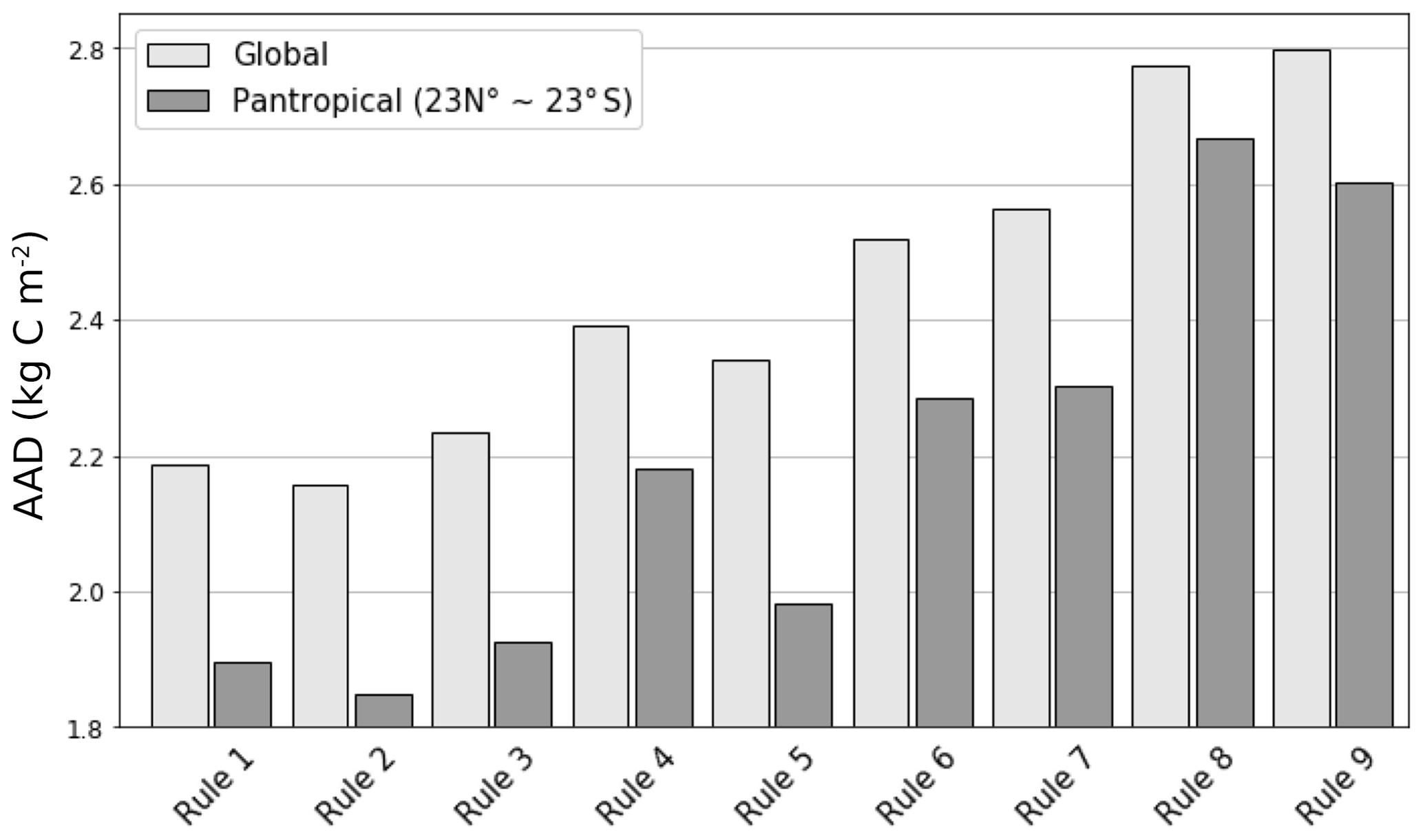
Figure 8 Average of absolute difference in carbon density between estimations of the nine translation rules and two diagnostic maps: global comparison with IPCC Tier-1 biomass density map (incl. above- and belowground); tropical comparison with Baccini's carbon density map (only aboveground).

A key feature of this study is to explicitly link land-use change and land-cover change and to provide insights into the consequences of choosing different land-use translation rules in ESMs. This study quantitatively characterizes historical land-cover change using the same underlying model of the LUH2, namely the GLM2. Estimates of forest cover and vegetation carbon between translation rules could provide information about sensitivities of ESMs to the LUH2 implementation. For example, in spite of the same land-use transitions from the LUH2, Rules 1–4 still have a difference of 43 Pg C in LULCC emissions during 1850–2000. Such difference solely from land-use translation accounts for about 24 % of the range of estimated vegetation carbon changes during 1850–2005 between CMIP5 models (Jones et al., 2013). Another feature is the relatively extensive evaluation of the LUH2 translation with multiple diagnostic datasets. The diagnostic datasets used in this study could serve to evaluate forest cover range at global and country level in ESMs. Besides, this study also emphasizes the necessity of improving vegetation carbon estimates, especially in regions with low forest cover or vegetation carbon in order to further differentiate translation rules.

Figure 9 Total carbon stock grouped by forest fraction from the averaged satellite-based forest cover map. (a) Global (above- and belowground); (b) pantropical (aboveground).

In additional to the nine rules designed in this study, many other designs of translation rules are possible for LUH2 implementation in CMIP6 models such as spatially or temporally varied rules. It is important to note that the designed translation rules of this study are spatially and temporally constant, meaning land-use changes in different regions or years will result in the same land-cover change for a given translation rule and given land-use transitions. This simplification may result in errors in land-use change translation because impacts of land-use change on land cover could vary by region and time. Combination of spatially/temporally varied rules, and the LUH2 may produce better estimates of forest cover and carbon density than the nine rules of this study. However, spatially/temporally varied translation rules will potentially add complexity to the LUH2 implementation in ESMs. Meanwhile, identification of such rules is sophisticated and also requires diagnostics with historical coverage. Uncertainties in these diagnostics should be small enough in order to differentiate various translation rules.

The estimated forest cover and carbon dynamics are subject to the several assumptions being made, the land-use change dataset being used, the land-cover properties being evaluated, reference datasets and the models. This study used the LUH2 dataset because of its required use in CMIP6 and widespread use in other studies. The land cover properties addressed here include two critical variables (i.e., forest cover and carbon stock) due to their biophysical and biogeochemical significance. Multiple datasets based on remote sensing and other sources were selected for evaluation with the intention to provide a robust reference. The use of the GLM2 model was selected to provide the most internally consistent treatment of these issues given its role in producing the LUH2 dataset. Given these considerations, it is possible that different results could be obtained for different systems. Although multiple satellite-based land-cover datasets were included, they disagree on the presence or absence of forest over low-forest-cover regions such as shrublands and semiarid savannahs and on the discrepancies due to technical challenges and disagreement of forest definition. In addition, global vegetation carbon mapping is still challenging and uncertain mainly because of indirect proxies of biomass and paucity of in situ measurements and observations from space. Uncertainties in vegetation carbon diagnostics limit the evaluation of translation rules such as differentiation of Rules 1–3. Furthermore, dynamics of forest cover and vegetation carbon from past to present interact with climate change and increasing atmospheric CO₂, which are not considered in this study. Finally, the carbon emission estimates using the same translation rules and land-use change dataset may be different using other ESMs/DGVMs.

Future research is needed to investigate both the robustness of these findings and potentially identify even better implementations. The CMIP6 LUMIP study is designed to quantify some of these effects (Lawrence et al., 2016) through model intercomparison. Additional work on translation rules should include possible spatial/temporal varying rules, partial land clearing and more land cover variables (e.g., forest age, height, soil carbon and energy balance) and focus on Rules 1–3 differentiation with better diagnostics such as annual land-cover maps from ESA Climate Change Initiative (CCI) (Lamarche et al., 2017) and lidar-based aboveground biomass from NASA's Global Ecosystem Dynamics Investigation (GEDI) mission (Dubayah et al., 2020).