Evaluation of three new surface irrigation parameterizations in the WRF-ARW v3.8.1 model: the Po Valley (Italy) case study

Irrigation is a method of land management that can affect the local climate. Recent literature shows that it affects mostly the near-surface variables and it is associated with an irrigation cooling effect. However, there is no common parameterization that also accounts for a realistic water amount, and this factor could ascribe one cause to the different impacts found in previous studies. This work aims to introduce three new surface irrigation parameterizations within the WRF-ARW model (v3.8.1) that consider different evaporative processes. The parameterizations are tested on one of the regions where global studies disagree on the signal of irrigation: the Mediterranean area and in particular the Po Valley. Three sets of experiments are performed using the same irrigation water amount of 5.7 mm d⁻¹, derived from Eurostat data. Two complementary validations are performed for July 2015: monthly mean, minimum, and maximum temperature with ground stations and potential evapotranspiration with the MODIS product. All tests show that for both mean and maximum temperature, as well as potential evapotranspiration simulated fields approximate observation-based values better when using the irrigation parameterizations. This study addresses the sensitivity of the results to human-decision assumptions of the parameterizations: start time, length, and frequency. The main impact of irrigation on surface variables such as soil moisture is due to the parameterization choice itself affecting evaporation, rather than the timing. Moreover, on average, the atmosphere and soil variables are not very sensitive to the parameterization assumptions for realistic timing and length.

1 Introduction

Irrigation has a crucial role in increasing food production: while less than 20 % of cultivated land is irrigated, it accounts for 40 % of the global agricultural output (Bin Abdullah, 2006; Siebert and Döll, 2010). Irrigation is also responsible for 70 % of the global water withdrawal and 80 %–90 % of the consumption (Jägermeyr et al., 2015). In the context of increasing population and reaching sustainable living, food production must increase to both sustain the current levels and ensure a fair distribution (Bin Abdullah, 2006). However, only expanding the arable land is an unrealistic solution as the loss rate to urbanization, salinization, and desertification is already faster than the addition rate (Nair et al., 2013). Moreover, in the context of the rapidly changing climate, a shift in productions and cultivars has been already observed throughout the world (e.g., IPCC, 2014; Wada et al., 2013; Lobell et al., 2008b; Zampieri et al., 2019). Anthropogenic influence on local climate is not only related to greenhouse emissions or changes in land cover but also to land management practices. The practice that has the largest impact is irrigation (Kueppers et al., 2007; Sacks et al., 2009; Wei et al., 2013; Cook et al., 2015). This is extensively used in semiarid regions (Sridhar, 2013), such as the Mediterranean region (Giorgi and Lionello, 2008), and particularly during the summer growing period when possible.

Recent literature shows that irrigation mostly affects near-surface atmospheric parameters, such as air temperature (e.g., Kueppers et al., 2007; Lobell et al., 2008a; Boucher et al., 2004; Sacks et al., 2009; Aegerter et al., 2017; Ozdogan et al., 2009; Sorooshian et al., 2014; Guimberteau et al., 2012). The majority of the studies found that irrigation has a local cooling effect, between 0.05 and 8 K, which does not clearly impact the global annual scale (Sacks et al., 2009; Boucher et al., 2004; Lobell et al., 2006; Guimberteau et al., 2012). Kueppers et al. (2007), Puma and Cook (2010), and Qian et al. (2013) found that the irrigation signal has a strong seasonal variability, with a maximum impact during the dry seasons of dry regions. However, in some specific regions, such as southern Europe and India, the response to irrigation is less clear: Boucher et al. (2004) obtain an induced warming and Sacks et al. (2009) a cooling. However, it should be mentioned that a study with a later version (with respect to Sacks et al., 2009) of the CESM model by Thiery et al. (2017) found that the cooling is predominantly caused by an increase in evaporative fraction, with only a minor influence of reduced net radiation to the surface. This discrepancy in the causes was ascribed to the fact that, in the previous version of the atmospheric model (CAM3), convection was very sensitive to the surface latent heat changes (Thiery et al., 2017). The effects of irrigation go beyond the surface cooling, as it affects the surface energy partition (e.g., Cook et al., 2015) and thus the atmospheric dynamics (Guimberteau et al., 2012; Saeed et al., 2009; Tuinenburg and de Vries, 2017; Douglas et al., 2009; Saeed et al., 2009; Lee et al., 2011), water vapor content (e.g., Boucher et al., 2004), and finally precipitation (Pielke and Zeng, 1989; Deangelis et al., 2010; Bonfils and Lobell, 2007; Puma and Cook, 2010). Some of the regional studies did not find a significant change in the cloud cover (Kueppers et al., 2007, 2008; Sorooshian et al., 2011; Qian et al., 2013), while others did (Aegerter et al., 2017; Krakauer et al., 2016). In fact, most of the variation is caused by the different surface energy balance partitions between sensible and latent heat flux (Seneviratne and Stöckli, 2008) by increasing the supply of soil moisture available (Cook et al., 2010). Kueppers et al. (2007) found an inland irrigation-induced circulation pattern due to the contrast between the relatively cool, moist irrigated areas and adjacent warm, dry natural vegetation. Qian et al. (2013) found an impact of irrigation on the thermodynamic air mass properties, which might increase the probability of shallow cloud formation.

As mentioned, both global and regional modeling studies disagree on the magnitude and spatial pattern of these effects (Harding et al., 2015; Kueppers et al., 2007; Sacks et al., 2009; Lobell et al., 2006). Several studies ascribe the different impacts modeled to both the irrigation modeling (Leng et al., 2017) and/or the amount of water used (Sorooshian et al., 2011; Wei et al., 2013; Sacks et al., 2009; Lobell et al., 2009). The parameterizations vary depending on the study goal and model land surface process representation, but they can be divided into (i) irrigation as column soil moisture change and (ii) surface application. The first group includes the studies based on Kueppers et al. (2007) and Qian et al. (2013), where the soil is maintained at the saturation point during the growing season. Also Lobell et al. (2008a) keep the soil moisture at field capacity for the whole irrigated simulation period, while Tuinenburg and de Vries (2017) keep it at 90 %. Both Sorooshian et al. (2011) and Aegerter et al. (2017) do not saturate the soil column but use a certain percentage of the field capacity of the root-zone, respectively 25 %–90 % (depending on the cultivar) and 80 % (sprinkler scheme). Thiery et al. (2017) use the CLM irrigation scheme from Oleson et al. (2013), which applies water to the soil to a specified depth until it reaches the target value (for more information refer to the two studies). The second group includes Kioutsioukis et al. (2016), where the irrigation is the amount of water requested by the difference between evapotranspiration and precipitation, with no information about timing. Also in Sacks et al. (2009) and Cook et al. (2010) the irrigation water is applied to the surface directly and thus it is an input to the land surface model, which then partitions it between evapotranspiration and runoff. Another method by Aegerter et al. (2017) (flood) applies water, without specifying how at the surface, until the top layer is saturated for 30 min. While all these different ways to parameterize irrigation might be representative under the proper assumptions, none is yet implemented in the more widely used regional models, such as WRF. Most importantly, the schemes mentioned do not account explicitly for irrigation water amount as an input, and none of the studies described determined a posterior the water used so that it is possible to compare it with realistic estimations. It should be mentioned that CESM (in the CLM component) allows for calibrating one parameter to match empirically the annual irrigation amount to the observed gross irrigation water usage for a specific period (Oleson et al., 2013; Thiery et al., 2017; Leng et al., 2017). However, this irrigation implementation accounts only for evaporation from the soil, as it is applied by increasing the soil moisture. Leng et al. (2017) point out that irrigation amount and its parameterization are crucial to assess, understand, and quantify the irrigation signal at the regional scale. Most of the global study irrigation schemes are within a closed hydrological cycle, which means that the water is extracted from other components simulated within the model (e.g., de Vrese and Hagemann, 2018; Oleson et al., 2013; Leng et al., 2017; Cook et al., 2010). However, this is not true for the limited area models (e.g., Kueppers et al., 2007; Lawston et al., 2015; Aegerter et al., 2017). The main reason could be that regional models (and some of the general circulation models, GCMs) often do not have a complex hydrological model within the land surface scheme and rarely include any groundwater process.

This study aims to provide a parameterization methodology for irrigation within a limited area model which considers different evaporation processes. This parameterization allows for a choice of timing parameters to account for different irrigation management practices in different regions. In particular, we focus on one of the aforementioned regions where global circulation models have an uncertain irrigation impact: southern Europe and the Mediterranean area. Irrigation methods and water used in the Mediterranean region depend on several factors such as cultivar type, climatic conditions, and also water availability (Daccache et al., 2014). Only one subregion of the area is chosen due to the different conditions: northern Italy and in particular the Po Valley (shown later in Fig. 3). In this area, the majority of the water used to irrigate comes from surface water; the percentage varies depending on the source from 71 % (Fader et al., 2016) to 95 % (Ministero delle Politiche agricole alimentari e forestali, 2009). The remaining water is extracted from groundwater sources. Different methods are employed to irrigate the cultivars and for historical reasons the most common one used is the “channel method”: 52 % of overall methods (Ministero delle Politiche agricole alimentari e forestali, 2009) or 61 % (Fader et al., 2016). This method is common in this area due to its double function of irrigation and reclaiming. In fact, water is distributed by gravity-fed open channels and flows directly to the soil via siphons or gated valves into furrows, basins, or border strips (Van Alfen, 2014). The same channels are used to drain excess water when necessary. The second most common method is irrigation through “sprinklers”, both pivot and rain-like sprinklers (Ministero delle Politiche agricole alimentari e forestali, 2009), for which the percentage varies from 24 % to 25 % depending on the source. Fader et al. (2016) include also the “drip method”, with a usage of 14 % of the total, which is not included in the report from the Italian Ministry of Agriculture and Forest. Most of the water extraction for irrigation does not happen directly from the Po River, but from the secondary rivers within the same basin (Ministero delle Politiche agricole alimentari e forestali, 2009).

This work continues considerations from previous studies of the impact of irrigation during dry growing seasons and the concerns of common irrigation parameterization methods, which have tuning parameters. Firstly here, irrigation parameterizations are developed for the widely used Weather Research and Forecasting (WRF) model. The parameterizations are then tested separately with the aforementioned irrigation methods currently deployed in the region for constraining the water use. Consequently, the impact of irrigation on atmospheric and soil components is discussed for the chosen area and simulation period.

This study does not address any effect of irrigation on the canopy, which is one of the main phenological impacts. In fact, irrigation increases the leaf area index, especially during stress periods, allowing high values despite the lack of precipitation (Aegerter et al., 2017), but here we use a seasonally varying vegetation-based leaf area index from the land surface model.

2 Irrigation parameterization development

Irrigation processes are complex since they involve both a human-decision component and physical forcing. The work here aims to develop and implement an approach that allows the model to account for both the human management dimension and the physical response to the forcing. As irrigation method definitions differ when different geographical areas are considered (Leng et al., 2017), our study will characterize the different parameterizations by their water loss. This can occur during both the transport system and the application. The first part can be related to numerical weather prediction models only when the transport is performed through open or closed channels, which leads to water loss due to evaporation and/or infiltration. To account for such a component, the model must have the capability of representing river processes, which WRF has not. Therefore, only the second component of the efficiency, the water loss in the application, is considered for these parameterizations (similar to Leng et al., 2017). As previous studies pointed out, depending on the irrigation techniques, different physical processes have to be accounted for (Bavi et al., 2009; Uddin et al., 2010; Brouwer et al., 1990). For example, the sprinkler system loses water due to droplet evaporation and drift, as well as vegetation interception (Uddin et al., 2010; Brouwer et al., 1990). However, depending on the geographical area, the techniques themselves vary (Leng et al., 2017). In fact, for some regions sprinklers are associated with systems that apply the water right above the canopy, so the water loss due to droplet evaporation is minimal. The most used sprinkler system of other regions may be the center pivot sprinkler, which might need to consider droplet processes if the irrigated field radius is large enough. Therefore, the parameterizations are defined based on the processes considered to account for different regional interpretations. Specific names are used for simplicity to differentiate the schemes within the model itself and for testing. However, they are not necessarily intended as resembling techniques used in real cases.

The methods presented in the next paragraphs consider an increasing amount of evaporation processes after the water leaves the irrigation system. In particular, the main processes considered are represented in the scheme in Fig. 1.

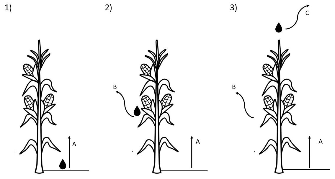
Figure 1 Irrigation schemes (1–3) with increasing evaporative processes considered (A–C): A is the evaporation from the water at the soil level, B is the canopy interception, and C is the drop evaporation and drift. This framework accounts only for surface water application and not subsurface.

In this framework, it should be noted that the water is introduced from a source that is considered not connected to the hydrological system. While the withdrawal source was found to have a key role from a theoretical perspective (Leng et al., 2017), WRF was not run with a hydrological component.

The implementation of the schemes within the WRF model are described in detail in the following part. The naming convention resembles the actual techniques for options 1 and 3, respectively CHANNEL and SPRINKLER. To avoid misrepresentation with option 2, the naming is chosen to recall the specifics as “DRip on leaves as Precipitation” or DRlP.

2.1 Option 1: CHANNEL

This method accounts only for evaporation from the soil and water at the surface (process A of Fig. 1), and the equations describing it are defined by the chosen land surface model. The irrigation water is added in the surface rainfall variable, and it is given to the land model as an input parameter. Therefore, this modification does not affect the atmospheric and vegetation parameterizations or equations directly but only indirectly.

For simplicity, the water used for the irrigation is defined, from an input, as an average daily amount expressed in millimeters (irr_daily_amount: V_I in mm d⁻¹, which is then converted to mm s⁻¹). Moreover, irrigation is set to start at the UTC time defined from irr_start_hour and it is partitioned equally during the consecutive irr_num_hours hours (h_I, converted in s). To conform with precipitation, W_I (mm s⁻¹) is expressed as

$$\begin{array}{}\text{(1)}& W_{\mathrm{I}}={\displaystyle \frac{V_{\mathrm{I}}}{h_{\mathrm{I}}}}{T}_{\mathrm{I}}.\end{array}$$

The obtained amount of water W_I is then integrated into the model time step. T_I is the irrigation interval, expressed as absolute number of days, which accounts for non-daily cases (see Sect. 2.5). This variable is used to compensate for the water quantity during the period when the irrigation method is not applied. This is the easiest way to have a fixed total amount of water for a simulation, which considers different irrigation frequencies. When the model time is in the irrigation interval defined by the start hour, h_I, and T_I, W_I is constant and defined as Eq. (1). Outside this interval, W_I is set to zero. A start and end day for irrigation can be defined using the Julian day calendar representation.

The evaporation processes that irrigation water undergoes are defined only by the land surface scheme chosen. There is no canopy interception in this method; therefore, the irrigation is not included in the canopy water balance.

2.2 Option 2: DRlP

This representation also allows for the water interception by the canopy and the leaves (process B in Fig. 1). In particular, it considers the water as applied right above the canopy. Once on the canopy, the water can undergo evaporation from the leaves and/or drip to the ground. The specific processes included in the representation of water intercepted by the canopy depends on the land surface scheme itself.

This scheme uses the same approach to include irrigation, i.e., via the surface precipitation, as the previous option. However, differently from the previous one, the water undergoes all rain processes related to canopy water balances. For example, if the land surface scheme allows a partition of the rain between interception and dripping, option 2 will include the interception, but option 1 will not.

2.3 Option 3: SPRINKLER

This option includes the droplet evaporation and fall processes (process C in Fig. 1), which in WRF are described in the microphysics schemes. Here, the irrigation is considered water sprayed into the lowest part of the atmosphere, namely the first full model level above the ground. The specific processes that the irrigated water undergoes in the microphysics depend on the choice of the scheme itself. However, all include the evaporation of the rain droplets, as well as advection and fallout.

This method assumes a static input of irrigated water directly into the rain water mixing ratio (a field that is updated in all schemes) as mass within the volume grid point. This avoids the need for any assumptions such as the falling speed or droplet size distribution. Therefore, the new rain water mixing ratio (Q_r, kg kg⁻¹) includes the irrigation in the lowest model layer as

$$\begin{array}{}\text{(2)}& Q_{\mathrm{r}}=Q_{\mathrm{r}}+Q_{\mathrm{I}}.\end{array}$$

The total grid point mass rate of water (m_I, $\mathrm{kg}{\mathrm{m}}^{-\mathrm{3}}{\mathrm{s}}^{-\mathrm{1}}$) added to the lowest mass level (Δz_ks, m), per cubic meter, is

$$\begin{array}{}\text{(3)}& m_{\mathrm{I}}={\displaystyle \frac{W_{\mathrm{I}}}{\mathrm{\Delta }{z}_{ks}}},\end{array}$$

where W_I has already been defined in Eq. (1). If Eq. (3) is divided by the lowest mass level air density ($\mathit{\rho }(t{)}_{i,j,ks}$ mass per cubic meter), it leads to the irrigation mixing ratio (Q_I, in $\mathrm{kg}{\mathrm{kg}}^{-\mathrm{1}}{\mathrm{s}}^{-\mathrm{1}}$):

$$\begin{array}{}\text{(4)}& Q_{\mathrm{I}}(t{)}_{i,j,ks}={\displaystyle \frac{W_{\mathrm{I}}}{\mathrm{\Delta }{z}_{ks}\mathit{\rho }(t{)}_{i,j,ks}}}.\end{array}$$

This value obtained is integrated into the microphysics time step, so it then has units of kg kg⁻¹ before adding it to the rain mixing ratio.

With this option, the microphysics scheme calculates the evaporation processes that irrigation water drops undergo exactly the same as rain droplets. After this, the irrigation water enters the model workflow as part of the microphysics precipitation field. Therefore, it is subject to the evaporation processes from canopy interception (process B) and the soil (process A) as they are described in the chosen schemes.

2.4 Irrigation mask field

The Food and Agriculture Organization of the United Nations (FAO) AQUASTAT database (Siebert et al., 2013) is used to increase the precision of where the irrigation takes place. This global gridded dataset combines national level census data of agricultural water usage for areas equipped for irrigation, with a resolution of 0.0833^∘ (around 9.24 km at midlatitudes). The dataset is included in the “geogrid” WPS (WRF Pre-Processing System) preprocessing as an optional field, giving the percentage of irrigated land within the volume grid cell. This allows the field to be interpolated consistently with all the other geographical ones to the chosen grid resolution. The water applied for irrigation, as described in the previous methods, is weighted by the percentage of irrigated land within the grid point.

2.5 Irrigation frequency greater than daily

As previously mentioned, the irrigation interval can be different than daily. This choice leads to a different behavior than having a sub-grid variability of irrigation, which would result in a lesser water amount used per grid point. In fact, it allows for investigation of the transition of the soil between intense irrigation states and days without any.

We can define two regimes accordingly to the interval: synchronous or non-synchronous. In the case of the synchronous irrigation, the chosen method is activated for the whole domain with the timing chosen by the combination of T_I, irr_start_hour, irr_num_hours, and irr_start_julianday. In fact, the active day has to be a multiple of T_I counting from the irrigation starting day. In the case of non-synchronous irrigation, the grid cells have still the same interval (T_I) but different phases. This considers that, with a multiday interval, the whole area might not be irrigated at the same time but on different days within the period. This leads to the possibility of having different irrigation spatial patterns, here called activation field, which is a static random field. The Fortran RANDOM_SEED function is used to create a repeatable random array that is given to calculate the activation field with the RANDOM_NUMBER Fortran function. However, this option does not ensure a reproducibility of the random field across different compilers. An additional option, reproducible across compilers, is given to create a pseudo-random field as a combination of invariant fields.

3 Methods

3.1 Model settings

The numerical weather prediction model used is the nonhydrostatic Weather Research and Forecasting (WRF) model v3.8.1 (Skamarock et al., 2008). In particular, the Advanced Research WRF (ARW or WRF-ARW) dynamical solver is used for this study(Skamarock et al., 2008); hereafter, when referring to the model used, it is implied that it is WRF with the ARW solver. In the study, WRF is used to test the parameterizations first for a 16 d period and then for a longer one. Therefore, it is important that the domain is correctly forced by the boundary conditions in order to have a long continuous run. The forcing by the boundaries is used to keep the model on the right path where the domain of interest is sufficiently close to the outer domain boundary, so the nonlinearities intrinsic in the fluid dynamics and physics are constrained, and the model does not diverge much from analyses.

The initial and boundary conditions for atmosphere and soil are chosen from different model products. ERA-Interim is used for the atmosphere because it is a state-of-the-art atmospheric reanalysis. In particular, note that ERA-Interim is an ECMWF global atmospheric multidecade reanalysis product which uses a 6 h 4D-Var data assimilation system with both ground and upper atmosphere data sources (Dee et al., 2011). ERA-Interim has a spatial resolution of approximately 80 km (around 0.75^∘; it is a T255 spectral grid) on 60 vertical levels from the surface up to 0.1 hPa (Dee et al., 2011). This allows for nesting directly from the boundary conditions to a 15 km resolution domain without too much disparity in resolution. The Global Forecast System (GFS) 0.25^∘ product (National Centers for Environmental Prediction, 2015) is used for the soil initial conditions because of its similarity to WRF's Noah land surface model (LSM) in the parameterization and soil level discretization (Ek, 2003). This allows for a more consistent initial condition for the soil layer temperatures and moisture.

Moreover, the MODIS 15 arcsec (around 450 m resolution) dataset is used for the land-category definition in the studied area. This is the most accurate dataset available for this region. As introduced in previous studies, WRF has the capability to nest multiple domains in the same run, reducing the total computational time and improving local climate representation. The configuration chosen is centered on the Po Valley, and it is shown on the left of Fig. 2.

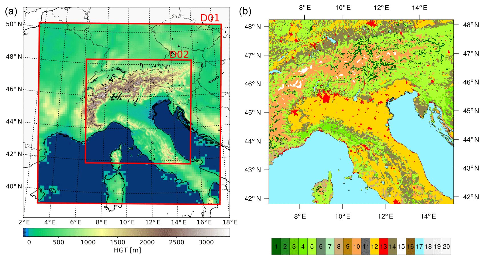
Figure 2 (a) shows both domains: the outer (D01) with 15 km grid resolution and the inner (D02) with 3 km. (b) shows the 20 land use categories used: numbers 1–5 represent different forest types, number 12 croplands, and 13 is built-up areas (for more information about the specific categories, refer to Skamarock et al., 2008).

The outer-most domain has a 15 km resolution and covers part of the northern Mediterranean area. The nested domain, called D02, has 3 km resolution and covers part of Italy and the Alps. The inclusion of the Alpine region in the higher resolution domain is meant to improve the complexity of the terrain representation and atmospheric behavior.

Given the above preprocessing choices, the parameterizations used are presented. The RRTMG (Rapid Radiative Transfer Model for GCMs) radiation scheme for both long-wave and short-wave radiation is used since it is commonly used in this area of interest (Mooney et al., 2013; Stergiou et al., 2017). The newer Tiedtke cumulus scheme is used for the outer domain that needs a convective parameterization; this parameterization is similar to the ECMWF cumulus scheme operationally used in the model (Zhang and Wang, 2017). This allows us to have a consistent cumulus parameterization with the boundary and initial conditions. The single-moment 6-class (WSM6) microphysics scheme (Hong et al., 2005) is used here due to its lesser computational cost with respect to others that have the same complexity. As in previous WRF studies, the YSU (Yonsei University) boundary layer parameterization is also used here (Hong et al., 2006). As mentioned before, the land surface model used for this study is Noah, which is the same model but different version of the one used in GFS (Saha et al., 2014; Tewari et al., 2004). The time step used for all schemes is the same as the model time step, which for the outer domain is 60 s and follows the 1:5 ratio for the inner domain, being 12 s.

The irrigation mask derived from the FAO dataset, for the Po Valley in the high-resolution domain (D02), is shown in Fig. 3.

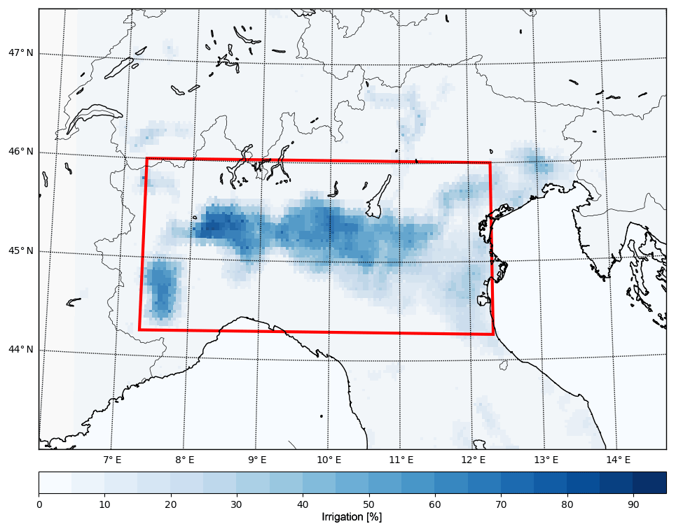
Figure 3 Percentage of irrigated area after regridding for the Po Valley. The red box highlights the averaging area used in this work.

As it can be seen, most of the western part of the Po Valley has more than 60 % of the land irrigated. The eastern side has lower irrigated percentages.

3.2 Test case: summer 2015, Po Valley

As mentioned before, the impact of irrigation is greater in drier and warmer seasons, so the irrigation signal is not masked by precipitation or larger-scale systems. Summer 2015 was a particularly dry and warm season, with a potential soil moisture deficit due to winter precipitation anomalies. While June 2015 was an average month with respect to the period 1981–2010, July was exceptional (ARPAE, 2015a, b). In fact, for the eastern part of the Po Valley, the temperature maxima were 1.8 ^∘C above those measured in July 2003 during the famous heat wave (for more about the 2003 heat wave, refer to Della-Marta et al., 2007, or García-Herrera et al., 2010). July 2015 registered negligible precipitation on the eastern side of the Po Valley, and the return period associated with the experienced soil moisture deficit is between 20 and 50 years (ARPAE, 2015b).

The irrigation water amount is derived for the area of interest shown in Fig. 3. The total amount of water used is 8.209×10¹² L (Eurostat, 2013), which is distributed on 1.5505×10¹⁰ m². The area considered already accounts for the percentage of irrigated land within the grid point as defined by FAO. It is assumed that irrigation is applied every day from 15 May to 15 August, for a total period of 92 d, to have a uniform temporal behavior. Therefore, the total amount of irrigation used in the region is 5.7 mm d⁻¹. The total water amount used for irrigation through the experiments will be the same, since the water amount is normalized (Eq. 1).

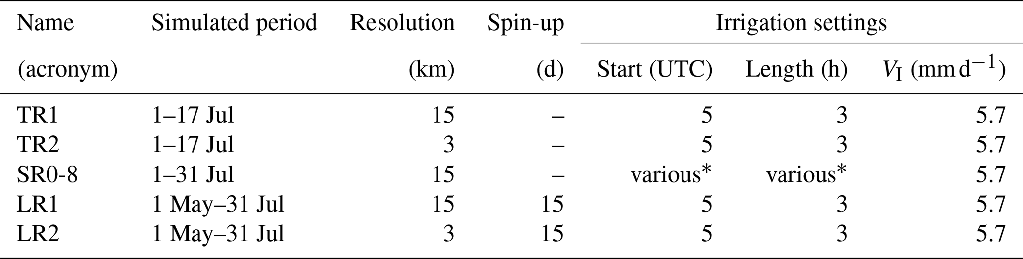
Several experiments are performed for different spatial resolutions and temporal periods to address the effect of irrigation on the local climate. Even though the periods might be different, they all include at least part of July 2015. Only runs that have the complete averaging period are included in the validation processes for averaging purposes. All the experiments are summarized in the Table 1. Each experiment is then described in detail below.

Table 1 Table with the experiments used in this paper: the main features of them are summarized here. For further explanations, refer to the main body text.“various^*” refers to the various settings that for simplicity reasons are described in Table 2.

3.2.1 Test run (TR)

This part of the experiment uses a subset of summer 2015, due to the high anomalies registered in the region: from 1 to 17 July at 00:00 UTC. The water amount is then distributed every day from 05:00 UTC (07:00 LT, local time) for 3 h, only in the inner domain. The irrigation is applied throughout the whole simulation period, without a spin-up time; therefore, the start and end day are not relevant.

Such a short period of simulation is used to test the scale dependency of the results. In fact, these settings are applied once to the outer domain (TR1) and once only to the inner domain (TR2). The TR1 is used to test the schemes at the 15 km resolution only, while TR2 has the schemes only in the convection-permitting D02 domain.

3.2.2 Sensitivity with coarse domain (SR)

This part of the experiment is used to test the dependency of the results to the starting time and irrigation length. The sensitivity study is done with the 15 km domain and for the month of July 2015 due to computational constraints. This ensures a high number of sensitivity members for different irrigation options. Table 2 summarizes the design of nine different settings that are applied to all three parameterizations. The chosen reference irrigation scenario, called “standard run”, is indicated with the number zero. There is also a control run with no irrigation. Therefore, the sensitivity has a total of 27 tests plus a common control simulation (CTRL SR). The starting time values are divided between early morning and late afternoon; one test is performed also for the middle of the day. More intuitive are the choices to irrigate either earlier in the morning or later in the afternoon: the water loss by evaporation and evapotranspiration is minimized and therefore the plant uptake is maximized. Combination 2 (start at 12:00 UTC) ensures that the representation of one of the least favorable irrigation conditions is also captured. In fact, during noon time the high temperatures in both soil and atmosphere are favorable to water evaporation. Combinations 3–6 change the length of application, varying the intensity to keep the same total amount.

Table 2 Table of number indexes used, e.g., CHAN4 is channel method fourth combination of the table here.

These sensitivity settings are also used to test the nonuniform temporal feature of the parameterization implementation, which are highlighted in the second part of Table 1. In the first of these tests, irrigation is activated every 3 d (combination number 7 of Table 2) and the second test every 7 d (combination number 8). Here, only the random static field approximation is tested since the configuration does not differ much from the pseudo-random one. As previously described, the frequency in days determines the activation field. For clarity, both activation fields are shown in Fig. 4. The values represent the number of the day within the sequence repetition in which the irrigation will be activated. For example, if a grid value is zero, it means that irrigation will happen on the first day of the interval between irrigation times.

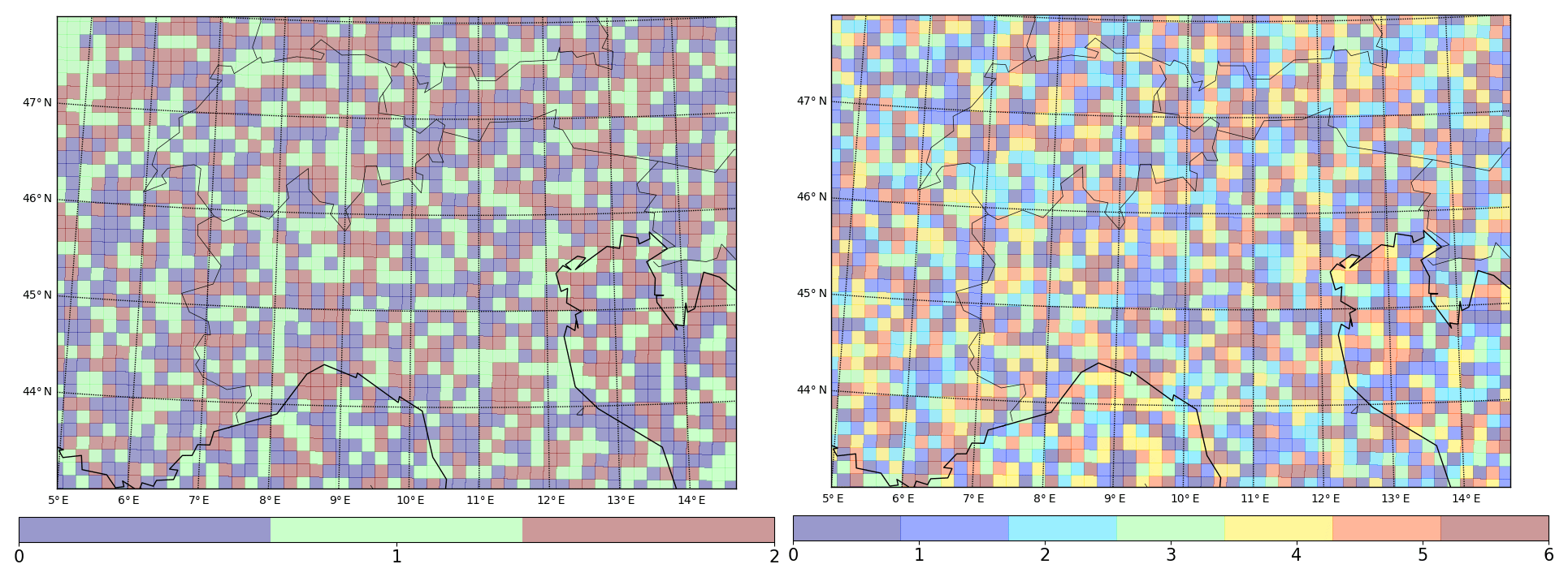
Figure 4 Activation field in days since the start of the sequence counting and highlight of the Po Valley region.

3.2.3 Long run (LR)

This set of experiments is done to address the longer-term influence of the developed irrigation parameters. The period simulated started on 1 May 2015 and ended on 31 July 2015. This simulation set uses only the moths of June and July for the analysis, as May is considered spin-up. This means that for the control, the soil moisture has a spin-up time of 31 d. However, in the case of the irrigated runs, the first 15 d are without the schemes active, and then 16 d are for irrigation to reach a new equilibrium. The water amount used is 5.7 mm d⁻¹, which is the same as all the other experiments. The long run experiment has the so-called “standard configuration”: every day from 05:00 UTC for 3 h, which was also used for the TR experiment. The aforementioned settings are used for both a high-resolution simulation (LR2) and a coarse one (LR1), for all three parameterizations and a control run.

In this study, this experimental setting is used only to validate the parameterizations. More in-depth analysis of the high-resolution results is out of the scope of this paper.

4 Validation

The validation of the parameterizations included in WRF consists of using surface station 2 m temperatures and satellite potential evapotranspiration. Data from the stations are from the regional weather services (ARPA, Regional Agency for the Protection of the Environment, from the regions Emilia-Romagna, Lombardy, and Piedmont) and have an hourly frequency. From all the available stations, only the non-urban ones are used. The potential evapotranspiration is a product of the Moderate Resolution Imaging Spectroradiometer (MODIS) Terra dataset (Running et al., 2017). Both validations are performed over monthly data due to the difference frequency in the original data, as well as the lack of diurnal information about irrigation.

4.1 Surface network of monitoring weather stations

Previous studies reported that irrigation affects the temperature; Kueppers et al. (2007) found an impact on the maximum diurnal temperature but no clear effects on the minimum one. Therefore, this first part of the validation consists of comparing the high-resolution long run (LR2) model output to the surface data. Of the 3 months in the LR2, only the last one is used for the validation: July 2015. As previous studies showed, dry months have a stronger irrigation signal (Kueppers et al., 2008; Leng et al., 2017). Therefore, the model results are affected more clearly by the parameterizations, and it helps to isolate the signal.

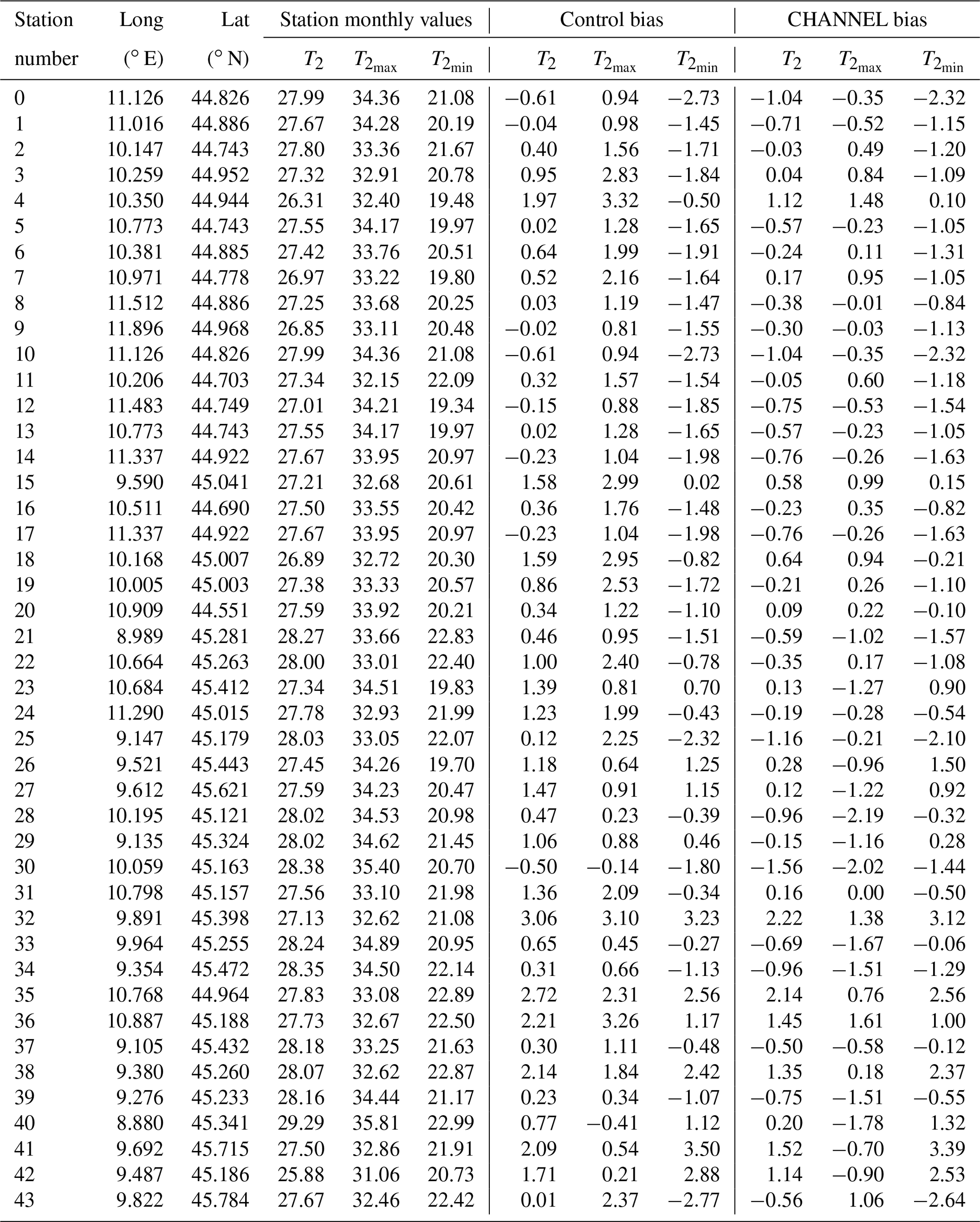
A bilinear interpolation is performed using the station coordinates to approximate the model gridded data to their locations. If in the interpolation the model land use category is not cropland, then the station is not used. This ensures that the model point results are not influenced by other land use physics, such as urban. Even though this should ensure that all stations and model points are actually in agricultural fields, the reality of the station locations is different. This is especially true for the ARPA Lombardy stations, where not all are standard WMO (World Meteorological Organization) stations or representative of their surrounding environment (e.g., station 37, as later explained).

Moreover, to ensure that the stations have a sufficient number of data for the monthly average, only stations with at least 80 % of the hourly values are used. This constraint leaves 44 stations out of the 62 downloaded originally. The mean, median, and standard deviation of the biases are calculated to understand the behavior of the biases, defined as the difference between the model run value for the location and the respective station. The results of this are shown in Table 3.

Table 3 Indexes for the monthly biases of the mean T₂ and the mean of the daily maximum and minimum temperatures for the valid stations: mean ($\stackrel{\mathrm{‾}}{x}$), median ($\stackrel{\mathrm{̃}}{x}$), standard deviation (σ), percentage of stations with positive bias (β⁺) and percentage of stations with a bias less than $\left|\mathrm{0.5}\right|{}^{\circ }\mathrm{C}$ (β^*).

Two percentages are added to the aforementioned statistics indices: the stations with positive bias and the ones with a bias less than $\left|\mathrm{0.5}\right|{}^{\circ }\mathrm{C}$.

In addition to Table 3, the biases are plotted (in Figs. 5, 6 and 7) with a shading of the IRRIGATION field (Fig. 3) to spatially visualize the impact of the parameterizations implemented. This allows for visualization of the irrigation pattern along with the bias changes caused by the schemes.

The first thing highlighted by Table 3 is that irrigation affects the biases mostly concerning the mean and maximum temperature, but not the minimum temperature. This finding agrees with results of previous works, such as Kueppers et al. (2007). From Table 3, both the mean biases and the percentage of stations with positive bias are reduced significantly. On the other hand, the standard deviation of the biases is not strongly affected. All the methods lead to an over decrease of the mean 2 m mean temperature, with more stations having a negative bias than a positive one (β⁺), such as Fig. 5a. Despite that, the number of stations with a bias between $\pm \mathrm{0.5}{}^{\circ }\mathrm{C}$ (β^*) decreases only slightly compared to the control run, which agrees with Fig. 5. Some stations show a bias, up to 3 ^∘C, that is not strongly affected by the schemes, and they are the ARPA Lombardy stations previously mentioned. For example, the station 37 (Table A1) is located on the bridge above the Ticino river. Therefore, a strong bias is expected since the model does not have a water body in the area. The three stations (numbers 27, 41, and 43 of Table A1) are in an Alpine valley, which can lead to issues in the model itself, such as the representation of steep terrain and the atmospheric dynamics. Despite these external issues with the stations, the irrigation parameterization still improves the biases.

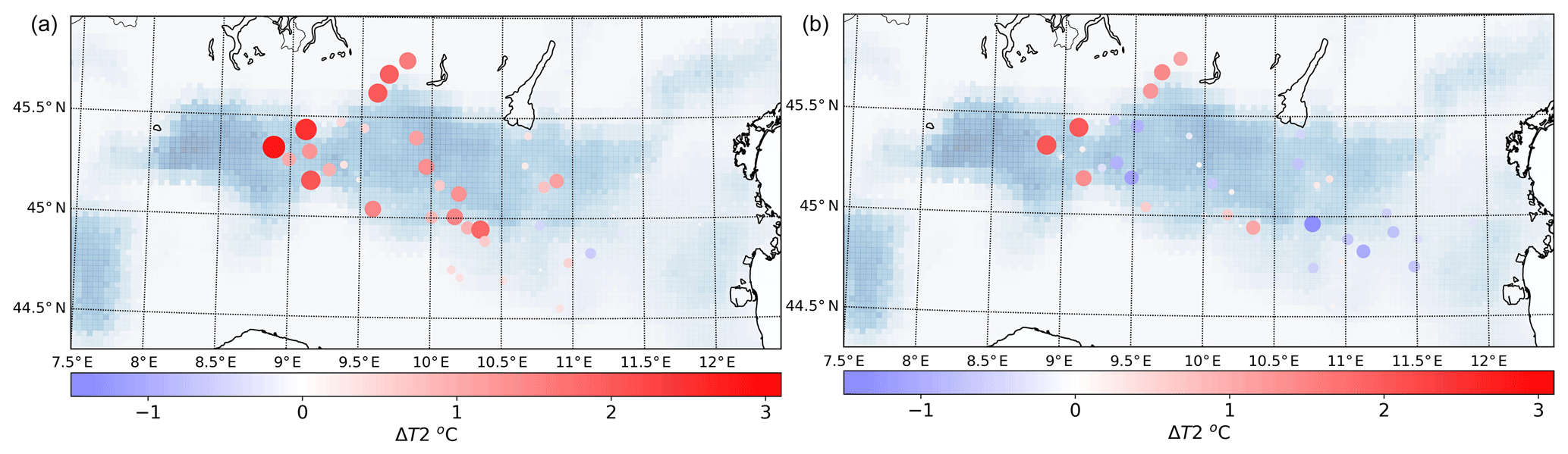
Figure 5 Monthly average for the 2 m mean temperature differences between the control (a) or channel (option 1, b) run and the weather stations at their locations. This is for July 2015 from the 3-month simulation (LR2). Both dot size and color represent the bias, and they are used combined to highlight high values.

Maximum daily temperature is the quantity that shows the best performance improvement. In fact, all indices show a significant improvement. The only exception is the standard deviation, which is not affected by the use of the irrigation parameterization. In particular, the control run has 95 % of the stations with a positive bias and only 14 % within $\pm \mathrm{0.5}{}^{\circ }\mathrm{C}$ (Fig. 6a). All the irrigation parameterization β⁺ and β^* values are closer to more optimal values. Interestingly for the maximum daily temperature, the mean is similar to the medians with the irrigation parameterization, which was not the case for the control run. This implies that it seems to improve the uniformity of the distribution of the biases, even though the irrigation field is not uniform. The CHANNEL and the DRlP parameterizations show similar spatial behaviors in the bias magnitude and distribution. The SPRINKLER scheme keeps more of the positive bias, being in general warmer than the other irrigation schemes.

Figure 6 Monthly average for daily maximum 2 m temperature difference between model run LR2 and the weather station locations for the control run (a), CHANNEL (option 1, b), DRlP (option 2, c), and SPRINKLER (option 3, d).

The monthly minimum daily temperature is the quantity least affected by the irrigation scheme. In this case, the statistics indices show almost no variation for the bias distribution due to the irrigation parameterization. In fact, the underestimation (β⁺) of the monthly minimum temperature does not change depending on the four runs. On the other hand, the mean and median values slightly improve with the irrigation schemes. The high standard deviation observed is caused by the ARPA Lombardy stations previously discussed, with a positive bias over 3 ^∘C in Fig. 7 (which are station numbers 41 and 42 in Table A1). In particular, the CHANNEL parameterization shows a bigger improvement of the negative biases in the southern part of the region observed in Fig. 7b. All the schemes do not significantly affect the positive biases in the irrigated area. Moreover, the SPRINKLER and DRlP schemes have a similar impact on the biases (Fig. 7c and d).

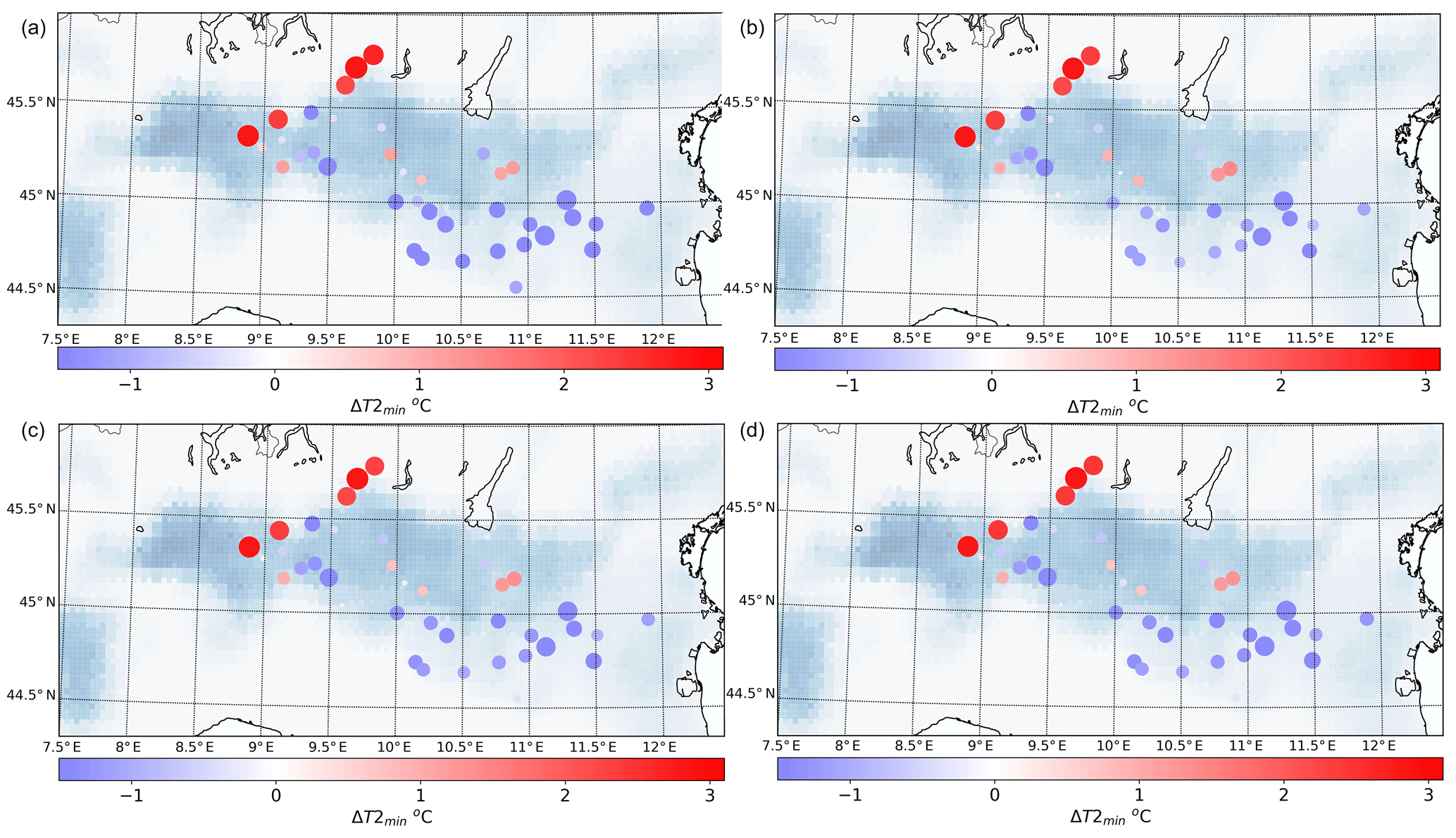
Figure 7 Monthly average for daily minimum 2 m temperature difference between model run LR2 and the weather station locations for the control run (a), CHANNEL (option 1, b), DRlP (option 2, c), and SPRINKLER (option 3, d).

4.2 Potential evapotranspiration

The potential evapotranspiration can be considered the evaporative demand from the atmosphere to the surface, as it is the maximum ability to evaporate under the assumption of a well-watered surface (Thornthwaite, 1948). As for satellite data, potential evapotranspiration is an indirect quantity, since it is derived from multiple measurements of satellite channels. Within the MODIS products there is also the evapotranspiration, which is the net effect between the evaporation demand and the availability. This could be a better quantity to estimate the effect of irrigation on the system. However, MODIS evapotranspiration is the result of a daily algorithm that combines both satellite measures and atmospheric models, as well as surface parameter assumptions (Running et al., 2017). Therefore, the assumptions of the evapotranspiration calculation makes the quantity not ideal for validation purposes.

The potential evapotranspiration (PET) from MODIS is an 8 d accumulated product, with a 500 m resolution, which is finer than the 15 and 3 km resolutions used in the model. Therefore, only the accumulated values for the whole irrigated area of the Po Valley are considered to compare such different scales. The potential evapotranspiration is summed for the whole July 2015 period because of the different temporal resolution between the data. The process is applied to the MODIS data, the sensitivity run (SR), and the long runs (LR1 and LR2). The results of the process are shown in Fig. 8. The accumulated value obtained for the MODIS data is 243 mm, which is from 33 % to 17 % lower than PET from the control run. All irrigated runs show an improvement of the potential evapotranspiration, decreasing the previous bias values to 23 % and 12 %. The highest improvement is observed in the 3-month simulations LR1 and LR2, of which only the last month is used. The potential evapotranspiration in the long control run (CTRL LR1) is higher than the one in the sensitivity control run (CTRL SR). In the case of the control run, SR and LR differ only for the spin-up time, as SR starts on the 1 July and LR is the 3-month simulation. Therefore the evolution to the equilibrium of variables with timescales longer than a few days, such as soil moisture, is longer. Nevertheless, the PET values are closer to MODIS in all experiments when the irrigation parameterization is activated. In particular, the differences in SR and LR control run PET are not observed anymore in the irrigated case of LR1 and SR0, so the irrigated runs have less spin-up effect or more quickly reach equilibrium Moreover, the potential evapotranspiration does not seem to be affected significantly by the start, length, or frequency of irrigation (SR experiments). There is some similarity between the same starting time, especially considering differences in PET between the schemes when irrigation starts at 17:00 UTC (cases 1, 5, and 6). However, such differences are very small compared to the quantities involved. Focusing on the frequency of the irrigation with the coarse domain, it is clear that it does not have an effect on the potential evapotranspiration. In fact, cases 7 and 8, respectively with frequencies of 3 and 7 d, are similar to cases SR0 and LR1.

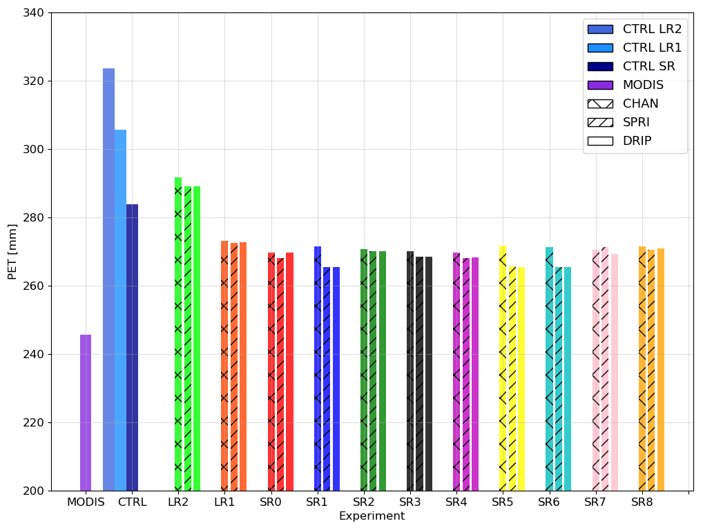
Figure 8 Monthly potential evapotranspiration accumulated for the irrigated area of the Po Valley (Fig. 3).

There is no significant difference in the accumulated potential evaporation depending on the scheme used, except that the channel (double hatching in Fig. 8) shows slightly higher values. Nevertheless, all irrigation schemes improve the accumulated potential evapotranspiration.

5 Results and discussion

5.1 Spatial influence of irrigation on soil moisture

Irrigation is applied to increase the water available to the plants; therefore, in modeling terms it has to influence the soil moisture in the simulation. Here the spatial soil moisture changes induced by the three parameterizations are presented and discussed. Since the irrigation perturbation is applied regularly every day or every several days and the temporal soil moisture scales are usually longer than that, we expect that some memory is retained. Pointwise differences in the fields are used to assess this quantitatively. This method allows for having both temporal and spatial averages of the differences by averaging in the corresponding dimension, without losing the spatial correlation of the introduced perturbation.

Firstly, we compare the soil moisture spatial differences of the long run, LR2, in the last simulated time step between the irrigated parameterization run and the control one (Fig. 9). All methods show a similar increase in soil moisture with respect to the control run and a spatial pattern that is clearly related to the irrigation field of Fig. 3. For agricultural purposes, all soil layers are important since the water needs to reach the roots. Therefore, in assessing the spatial impact of soil moisture (η) both the first and second level are shown, which are, respectively, 10 and 30 cm thick. In irrigated agriculture, the root zone tends to be more shallow than in the non-irrigated case due the lack of competition between ground and surface water sources (Lv et al., 2010). Therefore, the first two layers are enough to capture the real root zone. As can be seen from Fig. 9, both levels show an increase in soil moisture that is over 110 % for the first layer (on the left) and between 40 % and 90 % for the second one. The different increase rate in soil moisture between the layers is caused by the difference in timescales between infiltration and loss by evaporation and/or surface runoff.

Figure 9 Last model time step soil moisture percentage changes of the irrigated run (option 1, CHAN) with respect to the control (D02) for both the first soil level (a) and the second one (b).

Since the main changes in soil moisture are located within the irrigated zone, most of the time series will be done for a spatial average over that area alone.

5.2 Scale dependency of irrigation parameterization

The coarse domain is a more efficient way to run all the possible tests in terms of both computational costs and output storage, due to the high number of sensitivity combinations. However, the main variables must not vary much between different resolutions if influenced by the same irrigation methods, in order to use the coarse domain to run the sensitivity test. Therefore, the three schemes are run for both resolutions in the standard configuration as TR1 and TR2 to test the resolution dependence.

Two variables are considered when averaging over the irrigated area of both domains: the 2 m height temperature (T₂) and the soil moisture. While the use of soil moisture as a diagnostic has been previously discussed, the 2 m temperature is a common parameter for atmospheric studies. Moreover, from the physical perspective, this variable is influenced by both the ground state and the atmosphere. Therefore, it is an ideal parameter to consider when investigating surface perturbations.

In this part, both the time series (Fig. 10a, c) of the variables and the differences (Fig. 10b, d) between the different scales are shown. The latter are obtained as the differences between the field averages in different domains. So we subtract from the convection-permitting domain (D02) the value obtained in the convection parameterized one (D01). The results obtained are shown in the right column of Fig. 10 (Fig. 10b, d). The control simulation for TR1 and TR2 is added for the soil moisture field as well. When irrigation is activated, the soil does not dry as fast as in the control. The left side of the panel in Fig. 10 (Fig. 10a, c) shows that both variables have a similar behavior, within the spatial variability, in the two different scales. Since soil moisture is strongly affected by irrigation, which is not a spatially uniform field, high standard deviations are expected. This is the reason why the top right panel of Fig. 10 (Fig. 10b) does not show the standard deviation of either the high-resolution domain nor the coarse one. In fact, the differences in soil moisture between the resolution is at most 1 % of its value, and the spatial standard deviation is around 8 %. Therefore, differences in soil moisture due to resolution can be considered negligible. Regarding the temperature, it can be seen that the differences are mostly in the second part of the simulation, i.e., after 9 July when there was a weak frontal passage. Most of the differences between the resolutions happen during the nighttime, while daytime is less affected. One reason could be the cumulus scheme activation and its influence on the atmospheric state and dynamics. Nevertheless, the average behavior of the temperature fields are coherent with each other and with the different resolutions. Therefore, it is acceptable to use the coarse-resolution domain to understand the sensitivity of the parameterization timing assumptions, which will be shown in the next section.

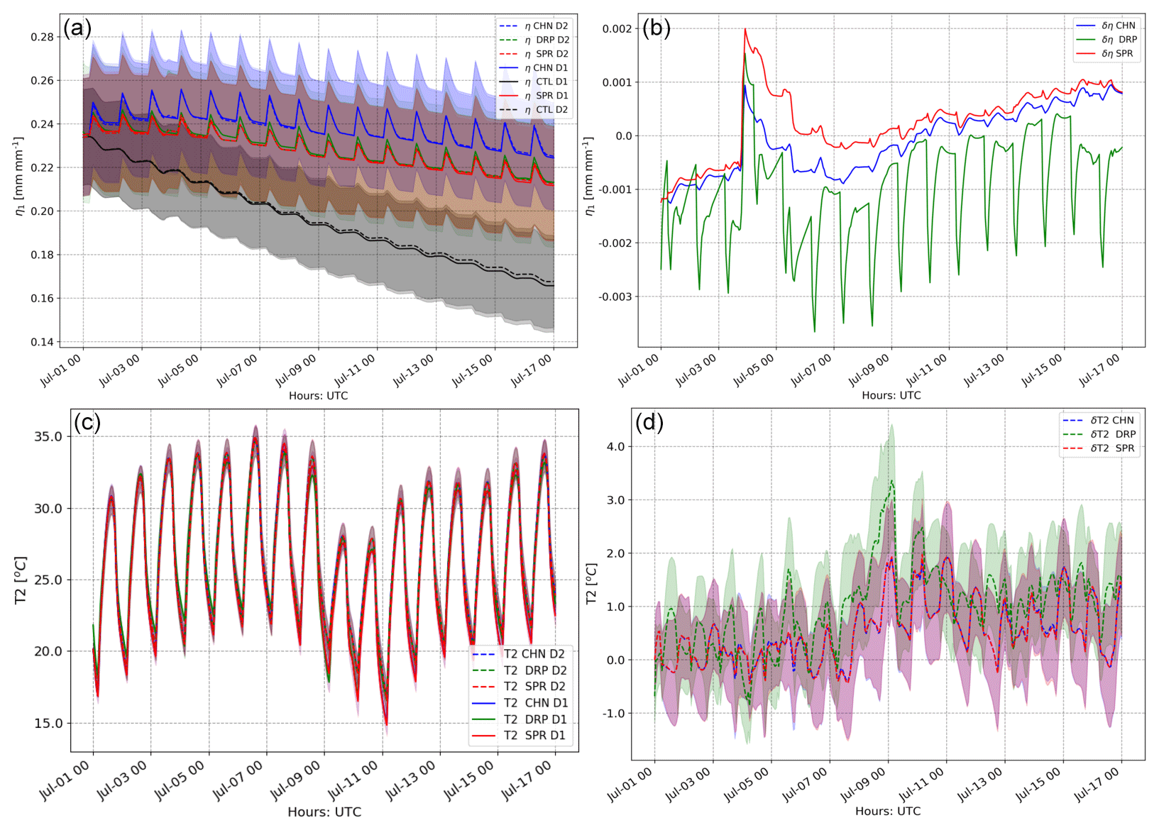
Figure 10 Time series of η (a, b) and T₂ (c, d) for both domains and all three parameterizations averaged over the irrigated area, with the spatial standard deviation as shading. The differences in the time series are calculated and plotted in the right side of the figure to highlight the differences between the resolutions. For the right panel, the shading represents the standard deviation of the differences.

5.3 Sensitivity

This part of the work discusses the sensitivity of the results to some of the parameterization options, such as the irrigation start time and length, as well as the frequency of the irrigation. This shows only the sensitivity run (SR) experimental settings (Table 2). Therefore, the SR nomenclature is dropped for now, so the parameterization and the case can be easily highlighted.

5.3.1 Differences from the control

First of all, the field time series of all the tests are shown in Fig. 11 as differences from the control run (which is the non-irrigated one) for both T₂ and η. All simulations increase the soil moisture content with respect to the control run. In particular, the left side of Fig. 11 (Fig. 11a) highlights how the major differences between the single tests are driven by the scheme type more than the timing. Clearly then, the CHANNEL method (blue lines) is the one that shows the biggest increase in soil moisture, while both SPRINKLER and DRlP do not differ greatly from each other. Therefore, regarding irrigation efficiency, the atmospheric evaporation in the SPRINKLER scheme is negligible if compared to the effect of the leaves and canopy interception, but the canopy interception is important in reducing the efficiency, meaning that re-evaporation from the canopy provides a noticeable loss.

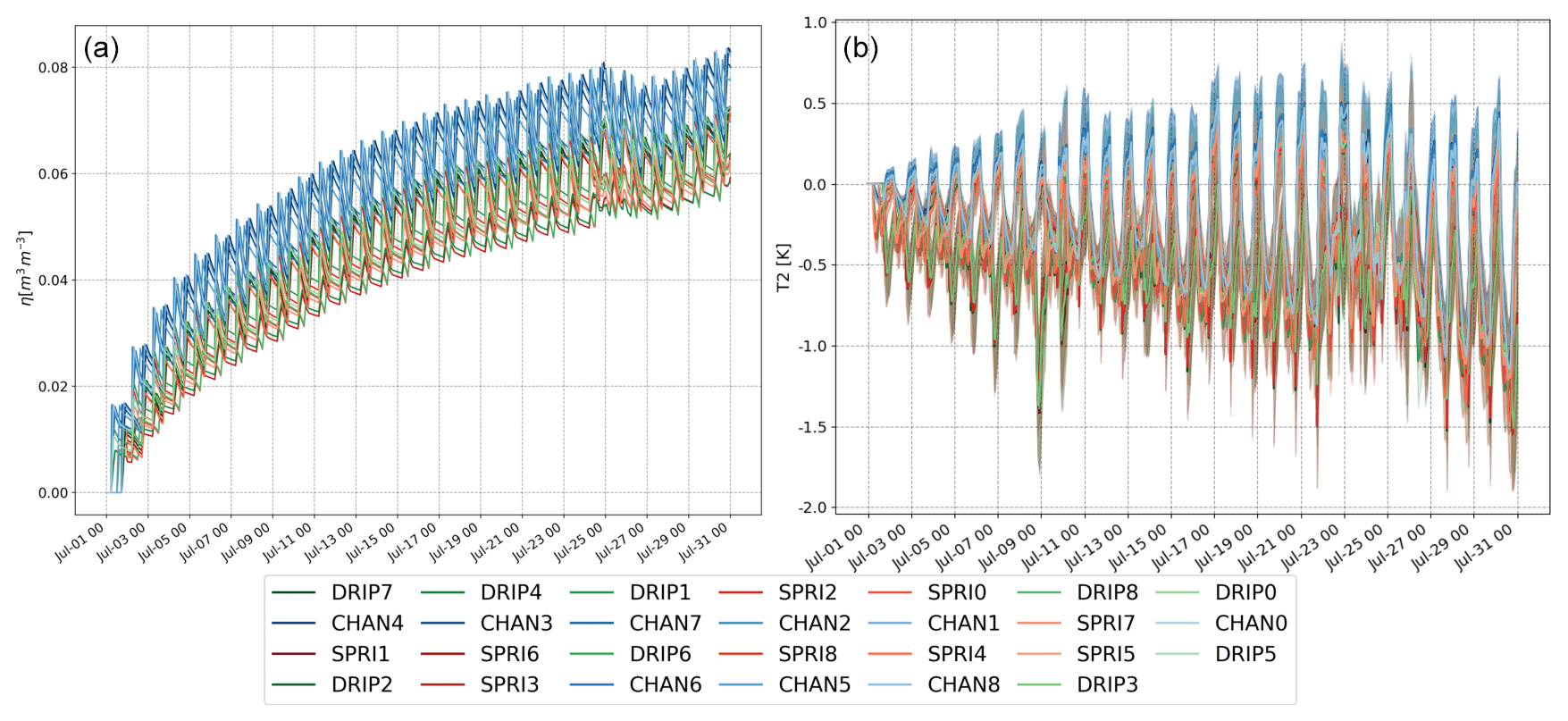
Figure 11 Time series of the differences from the control of all nine sensitivity tests averaged over the irrigated area. Soil moisture in (a) and 2 m temperature in (b). Blue colors shows the CHAN (option 1), green the DRlP (option 2), and red the SPRI (option 3).

The effect on 2 m temperature by the different assumptions is less evident than for soil moisture. In fact, most of the Δ T₂ time series on the right side of Fig. 11 show a decrease in the mean daytime temperature up to −1.5 K. It is noticeable how the nighttime temperatures of the CHANNEL parameterization are increased up to 0.7 K, while the other two are only up to 0.3 K.

The time series of the daily T₂ maximum (Fig. 12a) and minimum (Fig. 12b), for all runs, are considered in Fig. 12. The maximum daily T₂ is the quantity that is impacted by irrigation more clearly. For this quantity, all the SR irrigated tests behave very similarly by decreasing it with respect to the control run. The impact of the reduction of the maximum temperature is reduced outside the main heat wave period, namely during the frontal passages of 9 and 25–27 July. On the other hand, the minimum temperature seems less impacted by irrigation itself as well as its timing. All the SR tests behave similarly to the control, within the spatial standard deviation. Despite the fact that most of the irrigated SR simulations have higher minimum temperatures than the control, the values are within the standard deviation (shaded area in the plot). A probable reason for the warmer night temperature is the higher soil moisture: the higher η gives the soil a larger thermal inertia since it increases the heat capacity.

Figure 12 Time series of the daily maximum (a) and minimum (b) T₂ averaged over the irrigated area for all sensitivity tests and the control. Black color shows the CTRL run, blue the CHAN (option 1), green the DRlP (option 2), and red the SPRI (option 3).

In general, irrigation affects clearly the soil moisture and temperatures beyond the diurnal timescale of its application (Fig. 11). With this next part we are going to investigate if the timing itself has an influence beyond the daily application.

5.3.2 Diurnal cycle

Here the differences are taken with respect to the “standard” run (run 0) and not the control to analyze the effect of the parameterization's timing options more closely. This allows for isolating the effect of the specific choice on the soil and atmospheric variables. Since the effects in most of the tests have a daily frequency, the average diurnal cycle is discussed. Single days are also shown to understand the temporal variability of the perturbation on a daily basis, with the diurnal mean cycle. In this part, in addition to the previously presented T₂ and η, the heat fluxes (SH) and the upward moisture fluxes, as well as the soil temperature, are also included.

Figure 13a and b show that soil moisture differences from the standard are influenced by the timing and length of irrigation only regarding the peak location. Also in Fig. 13 the time series of the three standard runs as well as the control as a reference (lower panel) is shown. Firstly, it can be seen in the lower panel how the standard irrigated runs prevent the first layer of the soil from drying out, as happens in the control. While the control run soil moisture decreases from 0.24 to less than 0.16, for the irrigated runs it stays over 0.22 (on average). Also, notice that the CHANNEL parameterization soil moisture is always higher than both the SPRI and DRlP runs.

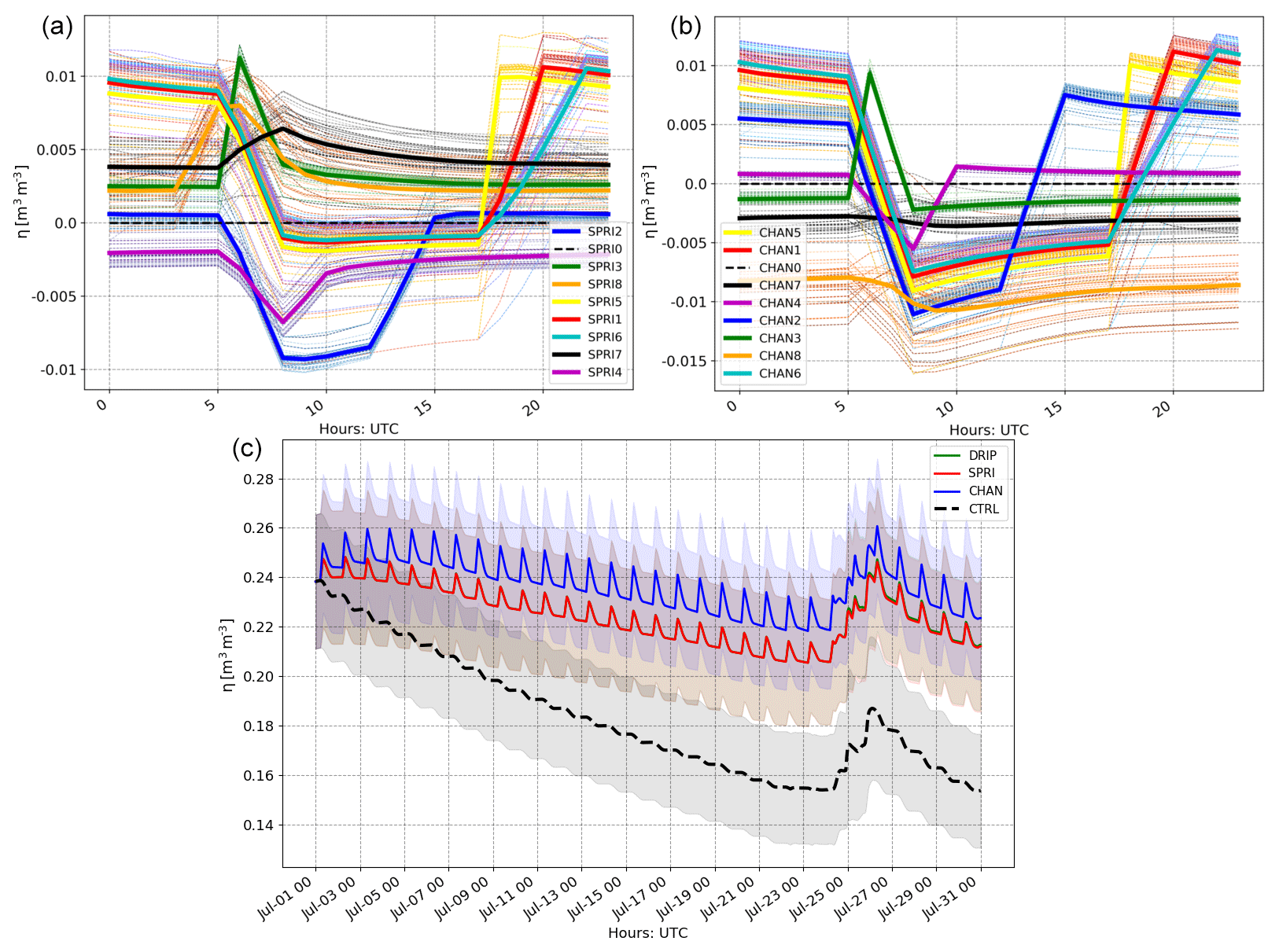
Figure 13 (a, b) Daily cycle of the mean first-level soil moisture difference between the test and the standard (run 0) shown by the solid line; the single day differences are the thin, dashed lines. Only two out of the three parameterizations are shown since there is no added information. (c) Time series of the three standard runs and the control.

Despite having different baseline values for the standard simulation, it is possible to see that the maximum in the differences from the standard (Fig. 13a, b) accounts only for up to 4 % of the total value. Moreover, the maxima in the differences are located according to the different irrigation starting times and lengths. Also, there is no long-term differences or multiday trend since the mean diurnal cycle agrees with the single daily cycles. On the other hand, the multiday non-in-phase irrigation is expected to have a slightly different behavior on a daily basis. Despite the fact that all grid points will be irrigated within the selected period (3 d for number 7 and 7 d for number 8), the percentage of irrigated land within the points is different. This will lead to having some single days with different diurnal cycle with respect to others, and it will reflect as a larger spread observed in the daily cycles (e.g., Fig. 13). Even though SR7 and SR8 have the same configuration as SR0, there is a change in the diurnal cycle. However, it is noticeable that such differences account only for less than 3 % of the total soil moisture amount. Therefore, a multiday frequency for irrigation does not seem to affect the longer-term soil moisture trends.

Given the expected anticorrelation between soil moisture and temperature, the opposite behavior seen in the differences of T₂ can be explained. However, when considering the larger-scale impact, T₂ could be used as an indicator of the atmospheric perturbation amplitude. Figure 14 shows the effect of timing and length on T₂ of the SPRINKLER and the DRlP parameterizations. Both parameterizations show a higher day-to-day variability relative to soil moisture, most likely due to the atmospheric state and dynamic influences. The bigger T₂ differences in the DRlP scheme are mainly in the nighttime with the late-afternoon irrigation starting time (Fig. 14b). On the other hand, the starting time at 12:00 UTC influences the daytime temperature more strongly in the SPRINKLER case than the DRlP one. This behavior is expected since the SPRINKLER experiment directly affects the atmospheric state via the microphysics evaporation process that would be larger in the daytime. Also, the difference between daily frequency in irrigation and the non-in-phase run are almost negligible with the DRlP (Fig. 14b) and slightly affected with the SPRI (Fig. 14a). A similar behavior to the DRlP is observed in the CHANNEL parameterization, which is not shown here, but the CHANNEL is warmer than the other two at night. While such differences in the night temperatures seem relevant for the local climate, they should be considered in the context of Fig. 12 (Fig. 12b). In fact, these magnitudes of 1 K are within the spatial variability of this quantity.

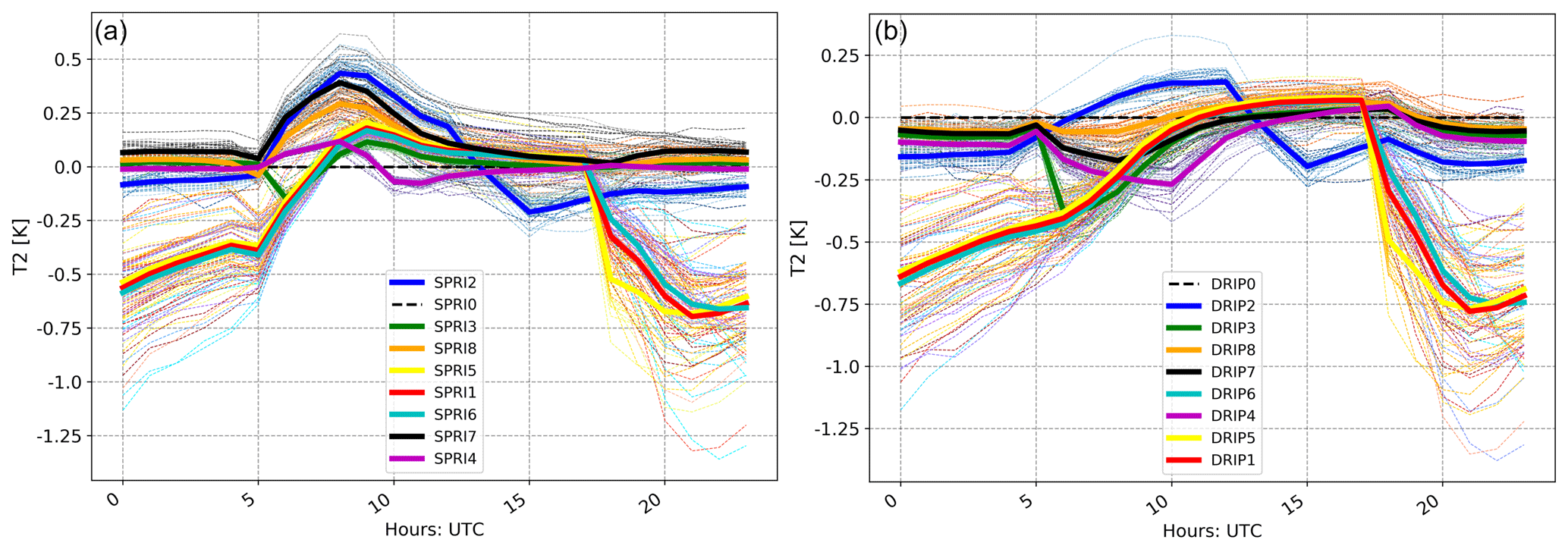
Figure 14 Same as Fig. 13a and b for the 2 m height temperature differences and a different set of parameterizations for the SPRINKLER (option 3, a) and DRlP (option 2, b).

This will affect the energy flux partition at the surface when considering a change in the soil state. This part analyses only the DRlP, since the behavior of the differences with respect to the standard run are similar for the other parameterizations. As for the soil moisture, the flux differences are also strongly affected by both timing and length, but only at the diurnal scale. In fact, there is no longer-term trend underlying the differences. The flux differences, Fig. 15a, show that the timing of irrigation impacts the fluxes mostly during the time when the parameterization is active. In particular, it is observed that the tests that differ most from the others are the ones where irrigation happens near the middle of the day (case numbers 4 and 2). Despite the differences from the other simulations, they account for changes of 12 % (E) and 20 % (SH) at most (Fig. 15).

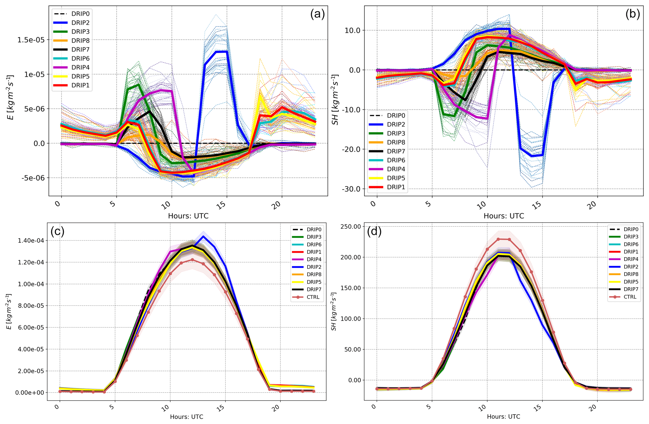
Figure 15 Same as Fig. 13; upward moisture and sensible flux for DRlP (option 2), respectively on the left and right sides, for the differences with respect to the standard run (a, b) and for the absolute values of diurnal cycle monthly average (c, d) including the control.

In the case of the afternoon irrigation (cases 5, 6, and 1), an increase in evaporation during most of the nighttime and a decrease during the daytime are observed. However, such decreases are usually small compared to the integrated increase. The described behavior is reflected during the daytime, with opposite sign, in the sensible heat flux differences (Fig. 15b). During the nighttime, on the other hand, there are no significant differences between the tests, as can be observed comparing the different tests in the lower part of Fig. 15.

Considering now all the dashed lines in the presented plots, it is possible to affirm that the timing does not have a great impact on the physical variables considered beyond their diurnal cycle. This affirmation is true also for the area averaged multidiurnal application (cases 7 and 8).

5.4 Evaporative loss from irrigation

The schemes account for different evaporative losses that can happen during the irrigation process after the water leaves the system used to deliver the water. As irrigation increases soil moisture, the evaporative loss is here defined in relation to the difference of soil moisture (Δη) with respect to the control run. The usage of the differences permits accounting for relative changes in the variables, disregarding the absolute values. Comparing the changes in the soil moisture in the different schemes allows for quantifying the water loss for each method.

As the schemes account for different evaporative loss components (Fig. 1), by comparing them in pairs, it is possible to isolate each term. The impact of the canopy evaporation (CANW) can be defined as the percentage change in the soil moisture field obtained with option 2 (DRlP) with respect to the option 1 (CHAN) and is calculated as

$$\begin{array}{}\text{(5)}& \text{CANW}={\displaystyle \frac{\mathrm{\Delta }{\mathit{\eta }}_{\text{DRlP}}-\mathrm{\Delta }{\mathit{\eta }}_{\text{CHAN}}}{\mathrm{\Delta }{\mathit{\eta }}_{\text{CHAN}}}}.\end{array}$$

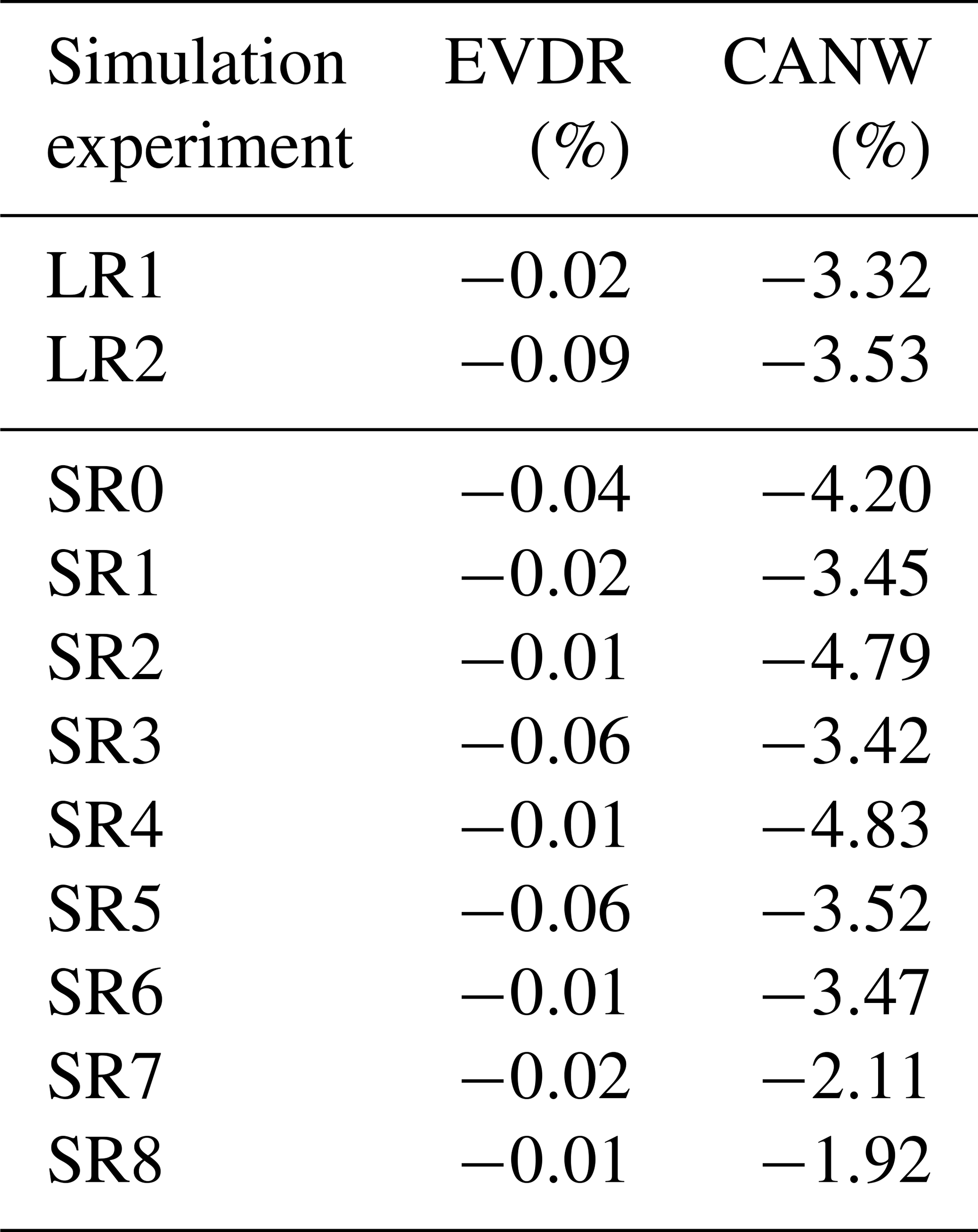
The same equation is used to calculate the impact of the microphysics processes (droplet evaporation and wind drift, EVDR) on irrigation, with the first term option 3 (SPRI) and the other option 2 (DRlP). This approach is valid under the assumption that irrigation is the only component of the model that affects the soil moisture field in the simulations. While it might not be true for all the time steps, it can give a more accurate interpretation if it is applied only during the irrigated hours. The results obtained averaging over the irrigated area (Fig. 3) and for the whole of July are shown in Table 4 below. The experiments show that the canopy/leaf interception effect is greater than the droplets evaporation and/or drift for all the experiments. A decrease around 4 % of the soil moisture is obtained if the canopy effect is considered. The average microphysics contribution causes a decrease in soil moisture below 0.1 % for all the experiments. However, it is noticed that the EVDR value is higher in the LR2 test, i.e., the convection-permitting long simulation. This highlights a possible stronger modification and coupling of the local conditions at smaller scales, which is investigated in a separate study. As the SR7 and SR8 represent the non-daily frequency, the averaging process includes points which are not irrigated. This is reflected by the lower impact of the CANW component but not on the EVDR one, which might be caused by the very low values.

Table 4 Evaporative loss expressed as soil moisture percentage change for the whole irrigated domain in July, due to EVDR, the impact of microphysics process (e.g., droplet evaporation), and CANW, the impact of canopy and leaves interception.

6 Conclusions

Agricultural land plays important economical and social roles, as well as influencing the local climate and biosphere. However, the land management change that impacts the local climate most is irrigation, if present. Recent literature shows that irrigation mostly affects the near-surface variables, creating the so-called irrigation cooling effect. This local cooling found by different studies is on average 1 K but can be up to 8 K, depending on the parameterization as well as the region. This study found a similar cooling impact of 1 K (with 1.03 K for the CHAN and 1.17 K for SPRI and DRlP) for the July spatial monthly average. However, the maximum in the temperature cooling for this region reaches 4 K. Such differences with previous limited area studies can be caused by the region and/or parameterization choices. The latter is found to be one of the uncertainty sources of the irrigation impacts on climate (Wei et al., 2013; Leng et al., 2017, e.g.,). Another source is the water amount applied, as none of the studies actually account for a realistic value. Several studies discussed that the lack of a common parameterization, as well as unknown total water amount applied, is the main cause of uncertainties.

This paper aims to present three new parameterizations for irrigation within the WRF-ARW model with an explicit water amount. These parameterizations define different surface irrigation techniques based on the evaporation processes that the water undergoes after it leaves the delivering system. Options 1 (CHANNEL) and 2 (DRlP) apply irrigation water as precipitation as an input to the land surface model. While option 2 allows for the interception of the water by the leaves and the canopy, option 1 does not. Option 3 (SPRINKLER) irrigation water is affected by the microphysics processes (such as droplet evaporation or drift), and it is introduced as a rain mixing ratio in the lowest atmospheric mass level of the model.

The current parameterizations are tested on one of the regions where global studies disagree on the signal of irrigation: the Mediterranean area. In particular, the Po Valley in northern Italy is chosen due to the dense irrigation system and the vulnerability to heat waves. For this area, summer 2015 was a good test-bed season for the agricultural months. In fact, while both summer months had positive temperature anomalies, their synoptic characterization was different. While July 2015 was an extreme month for high-temperature anomalies, lack of precipitation, and water stress, June 2015 was less extreme from the hydrological cycle perspective.

In this study, for clarity, the options are called with names that recall existing techniques or the specific behavior. In fact, option 1 is defined as the channel method, as it resembles that historical technique. On the other hand, option 3 is named as SPRINKLER, as the water is sprayed into the atmosphere and it uses the same assumptions of most of the irrigation studies within this discipline: the droplets might undergo evaporation and/or drift (e.g., Uddin et al., 2010; Leng et al., 2017). Option 2 is named DRlP, as the water used for the irrigation is applied over the canopy only and then it can be intercepted and drip to the ground. The terms here defined are not to be intended as a universal terminology, but as a naming convention within this study.

Three sets of experiments, with the same irrigation water amount of 5.7 mm d⁻¹, at the convection-permitting scale (3 km here) and/or parameterized (here 15 km) are performed for this warm summer season or part of it. The 16 d test run (TR) is used to assess the grid-scale dependency of irrigation's average field response. It is found that surface variables, such as 2 m temperature and soil moisture, do not show a different behavior depending on the model resolution. Therefore, a set of sensitivity experiments (SR) to irrigation start time, length, and frequency can be performed with the coarse setting. A long run (LR) of 3 months is used to validate the parameterizations against the surface temperature ground measurements from monitoring weather stations. Previous studies found that irrigation affects temperatures in both monthly averages of daily mean and maximum. Therefore, the parameterizations are tested against these quantities, as well as the minimum temperature. On average, the use of the irrigation schemes improves the model representation of these variables, reducing the biases. In fact, while for the control run the average monthly bias is 0.75 ^∘C for the mean and 1.46 ^∘C for the maximum temperature, the irrigation run biases are reduced, respectively, to $(-\mathrm{0.15}\pm \mathrm{0.06})$ and $(-\mathrm{0.13}\pm \mathrm{0.17})$ ^∘C averaging the three methods. The July potential evapotranspiration accumulated for the irrigated region of the Po Valley is evaluated for all nine sensitivity runs (SR0-8) and the long runs (LR1 and LR2). All tests show that the potential evapotranspiration is improved when the irrigation parameterization is used in the model.

The study also addresses the sensitivity of the results to the parameterization human-decision options: irrigation timing as start time (in UTC), length (in h), and frequency (in d). The main impact of irrigation on soil moisture and 2 m temperature with respect to the control is due to the parameterization choice itself rather then the timing. The CHANNEL method is slightly more efficient in terms of increasing the long-term soil moisture than the other two methods, but the similarity of the other two methods showed that the canopy interception is more important in reducing efficiency than the evaporation from the sprinkler process. Diurnal cycles of both atmospheric and surface variables are calculated as differences with respect to the standard configuration, namely when there is daily irrigation starting at 05:00 UTC and going for 3 h. No significant impacts beyond the diurnal timescale are found due to timing for soil moisture, sensible heat, and upward moisture fluxes. Assessing the impact on T₂ is more complicated, as the differences observed in the diurnal cycle are comparable to the ones that are obtained with different resolutions. With this sensitivity work, it is found that irrigation itself influences the physical quantities beyond the diurnal timescale of its application (so comparing the runs with the control simulation). However, the timing of irrigation does affect these atmospheric and/or soil variables only within the diurnal cycle. (It is done using the sensitivity tests and as a base the standard run, which is the combination number zero.)

The usage of an irrigation parameterization for this area improves the model representation. Moreover, on average, the atmosphere and soil variables are not very sensitive to the parameterization options for realistic irrigation timing and length. Therefore, the use of the standard configuration alone for the high-resolution long run is acceptably representative.

Further analysis on assessing the physical and dynamical impacts of the irrigation on the atmosphere is addressed in two follow-up works.

Appendix A: Surface weather stations monthly results

The values obtained for each station used in the validation section are written in Table A1. For clarity, the stations are identified with a unique number (from 0 to 43) and their geographical coordinates (not by their name). The temperature values refer to the values obtained from the gridded model output. The bias is obtained by subtracting the simulation value from observation from the station.

Table A1 Monthly averaged mean, maximum, and minimum values obtained for each station in Figs. 5–7.