Simulator for Hydrologic Unstructured Domains (SHUD v1.0): numerical modeling of watershed hydrology with the finite volume method

Hydrologic modeling is an essential strategy for understanding and predicting natural flows, particularly where observations are lacking in either space or time or where complex terrain leads to a disconnect in the characteristic time and space scales of overland and groundwater flow. However, significant difficulties remain for the development of efficient and extensible modeling systems that operate robustly across complex regions. This paper introduces the Simulator for Hydrologic Unstructured Domains (SHUD), an integrated, multiprocess, multiscale, flexible-time-step model, in which hydrologic processes are fully coupled using the finite volume method. SHUD integrates overland flow, snow accumulation/melt, evapotranspiration, subsurface flow, groundwater flow, and river routing, thus allowing physical processes in general watersheds to be realistically captured. SHUD incorporates one-dimensional unsaturated flow, two-dimensional groundwater flow, and a fully connected river channel network with hillslopes supporting overland flow and baseflow.

The paper introduces the design of SHUD, from the conceptual and mathematical description of hydrologic processes in a watershed to the model's computational structures. To demonstrate and validate the model performance, we employ three hydrologic experiments: the V-catchment experiment, Vauclin's experiment, and a model study of the Cache Creek Watershed in northern California. Ongoing applications of the SHUD model include hydrologic analyses of hillslope to regional scales (1 m² to 10⁶ km²), water resource and stormwater management, and interdisciplinary research for questions in limnology, agriculture, geochemistry, geomorphology, water quality, ecology, climate and land-use change. The strength of SHUD is its flexibility as a scientific and resource evaluation tool where modeling and simulation are required.

1 Introduction

The complexity of today's environmental issues, the multidisciplinary nature of scientific and resource management questions, and the diversity and incompleteness of available observational data have all led to the need for models as a means of synthesis. When models are computationally efficient and physically consistent, they become important tools for extrapolation across observations and systems. They help us better understand the physical history of a given system and make decisions about the future in light of socioeconomic, hydrologic, or climatological change. The datasets produced through modeling can assist with decisions for infrastructural planning, water resource management, flood protection, contamination mitigation, and other relevant concerns. Nonetheless, models of varying complexity are available, and the required model complexity (resolution, scale, and coupled states/fluxes) for a given problem depends on the particular research or management purpose, the questions to be answered, and the data available.

Nonetheless, environmental managers, policymakers, and stakeholders have a growing demand for high-resolution and detailed information about hydrologic flows at fine temporal–spatial resolution across watersheds. This need reflects the ever-increasing importance of detailed long-term predictions and projections for ecological systems, agricultural development, and food security under future climate change. Global climate modeling, typically performed with a general circulation model, also requires information on soil moisture and groundwater fluctuations, which are related to streamflow and reservoir management (Hrachowitz and Clark, 2017; Blöschl et al., 2019).

In hydrology, lumped models (Hawkins et al., 1985; Fleming, 2010; Bergström, 1992) have proven to be fast and stable tools for estimating the streamflow in rivers, requiring simplified meteorological data and limited observed flow data. Lumped models disregard the spatial heterogeneity of terrestrial characteristics while including the basic watershed features (e.g., contributing area, overall relief, average land use, soil conditions, etc.). Their purpose is input-output analysis without internal structure (Moradkhani and Sorooshian, 2008), and their parameters may lack precise physical meaning, which makes it challenging to interpret watershed characteristics or transfer parameters to other regions. On the other hand, distributed models (Beven, 2012; Lin et al., 2018; Gochis et al., 2015; Santhi et al., 2006; Liang et al., 1996; Vivoni et al., 2011; Refsgaard et al., 1998; Shen and Phanikumar, 2010) also have their limitations. One challenge for multiprocess distributed models is addressing uncertainties in spatial parameters (soils, hydrogeology, land-surface processes, etc.) and limited predictive skill for large, high-resolution catchments, even if the estimated model parameters (e.g., soil properties, surface characteristics, and aquifer properties) and atmospheric inputs have incommensurate resolutions. The latter is particularly important to watershed calibration and has led to a major source of uncertainty (Beven, 2012; Blöschl et al., 2019). Nonetheless, at the continental and global scale, progress has been made in higher-resolution elevation data, refined soil surveys (Soil Survey Staff, 2015), satellite land cover (Homer and Fry, 2012), and much higher-resolution atmospheric inputs. This has created new opportunities for the development of new hydrologic models that leverage advances in data and mathematical/computational strategies.

Communities have become more sophisticated about their choice of models (Beven, 2012) and tailoring models to explicit purpose or applications, with models ranging from the simplest lumped models (HEC-HMS, Fleming, 2010, HBV, Bergström, 1992) to semi-distributed models (Beven, 1989; Beven and Germann, 1982; Beven and Kirkby, 1979), complex distributed hydrologic models (WRF-Hydro, Lin et al., 2018; Gochis et al., 2015, PRMS, Leavesley et al., 1983, SWAT, Santhi et al., 2006, VIC, Liang et al., 1996, MIKE-SHE, Abbott and Refsgaard, 1996; Refsgaard et al., 1998, inHM, VanderKwaak, 1999, tRIBS, Vivoni et al., 2011, 2004, 2005 and PAWS, Shen and Phanikumar, 2010), and even cutting-edge hydrologic models based on machine-learning methods (Rasouli et al., 2012; Petty and Dhingra, 2018; Shen et al., 2018). In each case the choice of model requires the assessment of factors related to prediction variables, performance, flexibility, and availability of data.

The Simulator for Hydrologic Unstructured Domains (SHUD) is a multiprocess, multiscale model where major hydrologic processes are fully coupled using the finite volume method (FVM). SHUD encapsulates the strategy for the synthesis of multi-state distributed hydrologic models using the integral representation of the underlying physical process equations and state variables. As an intellectual descendant of Penn State Integrated Hydrologic Model (PIHM), the SHUD model is a continuation of 16 years of PIHM model development in hydrology and related fields since the release of its first PIHM version (Qu, 2004).

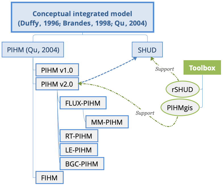
The conceptual structure of the two-state integral-balance model for soil moisture and groundwater dynamics was originally devised by Duffy (1996), in which the partial volumes occupied by unsaturated and saturated moisture storage were integrated directly into a local conservation equation. This two-state integral-balance structure simplified the hydrologic dynamics while preserving the natural spatial and temporal scales contributing to runoff response. Brandes et al. (1998) used FEMWATER to capture the inflow/outflow behavior within a hillslope–stream scheme. In 2004, Qu (2004) embedded evapotranspiration and river networks and released the Penn State Integrated Hydrologic Model (PIHM) v1.0, which was the most important milestone of the two-state integral-balance model. Since PIHM v1.0 (Qu, 2004), the PIHM has been a generic hydrologic model applicable to general watersheds or basins. After that, PIHM v2.0 (Kumar et al., 2009; Kumar and Duffy, 2009) enhanced PIHM's land surface modeling component. A GIS-tool, PIHMgis (Bhatt et al., 2014) and the Essential Terrestrial Variables Data Server (HydroTerre, Leonard and Duffy, 2013) accelerated model deployment and motivated additional applications with PIHM. Because of the sophisticated hydrologic modeling capability and efficient spatial representation in PIHM, various model coupling projects were later initiated. For example, Flux-PIHM coupled the NOAH Land Surface Model with PIHM to provide a more detailed calculation of energy balance and evapotranspiration (Shi et al., 2015, 2014). Zhang et al. (2016) coupled landscaping evolution with PIHM (LE-PIHM). Bao (Bao, 2016; Bao et al., 2017) added a reaction-transport module to PIHM (RT-PIHM, RT-Flux-PIHM). Flux-PIHM-BGC (Shi et al., 2018) provided biogeochemistry into Flux-PIHM. The Multi-Module PIHM (MM-PIHM) project (https://github.com/PSUmodeling/MM-PIHM, last access: 19 December 2019) was then devised to build a uniform repository for all coupled modules. Still, more PIHM coupling projects are ongoing, targeting sediments, lakes, crops, and other systems. Simultaneously, a Finite volume-based Integrated Hydrologic Modeling (FIHM) was also developed (Kumar et al., 2009), which used second-order accurate finite volumes and solved for both 2-D unsteady overland flow and 3-D subsurface flow. Figure 1 shows the family tree of PIHM and SHUD. Within this tree, essentially every revision/branch received cross-pollination from others, supporting the ever growing complexity of these systems. The PIHMgis (Bhatt et al., 2014) and rSHUD (Shu, 2020) are GIS, pre- and postprocessing tools for PIHM and SHUD, respectively. Although PIHM and SHUD share the same fundamental conceptual two-state integral model, both the inputs and outputs are incompatible. Details of differences between them are summarized in Sect. 4.1 of this paper.

Figure 1 The family tree of PIHM and SHUD. PIHM and SHUD share the same fundamental conceptual model but use different realization. The PIHMgis and rSHUD (Shu, 2020) are GIS-tools for pre- and postprocessing.

SHUD's design is based on a concise representation of a watershed and river basin's hydrodynamics, which allows for interactions among major physical processes operating simultaneously but with the flexibility to add or drop state-process-constitutive relations depending on the objectives of the numerical experiment.

As a distributed hydrologic model, the computational domain of the SHUD model is discretized using an unstructured triangular irregular network (e.g., Delaunay triangles) generated with constraints (geometric and parametric). A local prismatic control volume is formed by the vertical projection of the Delaunay triangles forming each layer of the model. Given a set of constraints (river network, watershed boundary, elevation, and hydraulic properties), an optimized mesh is generated. The optimized mesh allows the underlying coupled hydrologic processes for each finite volume to be calculated numerical efficiently and stability (Farthing and Ogden, 2017; Vanderstraeten and Keunings, 1995; Shewchuk, 1996). River volume cells are also prismatic, with trapezoidal or rectangular cross section, and maintain the topological relation with the Delaunay triangles. The local control volumes encapsulate all equations to be solved and are herein referred to as the model kernel. The R package rSHUD (Shu, 2020) has been developed to help users generate these triangular domains.

The objective of this paper is to introduce the design of SHUD, from the fundamental conceptual model of hydrology to governing hydrologic equations in a watershed to computational structures describing hydrologic processes. Section 2 describes the conceptual design and equations used in the model. In Sect. 3, we employ three hydrologic experiments to demonstrate the simulation and capacity of the model. The three applications presented here are (1) the V-catchment experiment, (2) the Vauclin experiment (Vauclin et al., 1979), and (3) the Cache Creek Watershed (CCW), a headwater catchment in northern California. Section 4 summarizes the differences between SHUD and PIHM, then proposes possible applications of the SHUD model.

Figure 2 The conceptual schematic of hydrologic processes in the SHUD model.

2 Model design

2.1 Conceptual description of hydrologic system

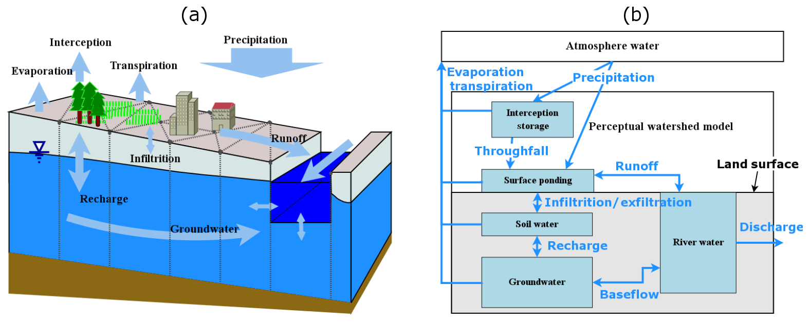
We begin our introduction to the SHUD model with a conceptual description of water movement in a watershed. Figure 2 depicts processes that are incorporated in the model. Catchment hydrology is driven by atmospheric inputs, including rainfall, snowfall, and irrigation. The land surface hydrology first interacts with vegetation through plant-canopy interception and throughfall. When precipitation exceeds the interception capacity, throughfall or excess precipitation falls to the land surface. Snowfall accumulation and melting is an important land-surface process and a major source of soil moisture and recharge in many temperate or mountainous climate regions. SHUD captures the partitioning of excess precipitation into surface runoff and infiltration into the soil.

Vertically, the aquifer is divided into two coupled layers based on its saturation status: the top unsaturated layer (or vadose layer) is constrained to 1-D vertical flow, and the saturated groundwater layer admits 2-D flow. These layers overlie an impermeable or low-permeable layer such as bedrock or an effective depth of circulation where deeper flows are small and unlikely to contribute to baseflow. The vertical fluxes within the unsaturated zone include infiltration and exfiltration. Deep percolation or recharge to groundwater is fully coupled to soil moisture dynamics. SHUD accounts for conditions when the groundwater table reaches or exceeds the land surface, decreasing infiltration, allowing exfiltration as local ponding and runoff. The model also accounts for upward capillary flow from a shallow water table depending on soil moisture and vegetation conditions. Lateral (2-D) groundwater flow represents the basic mechanism for baseflow to streams or rivers.

Surface runoff or overland flow is generated by excess rainfall and ponding and is represented as 2-D shallow water flow in SHUD. Surface runoff complements baseflow runoff as the dominant source of streams or rivers. SHUD also allows reversing flows from the channel to the hillslope as surface inundation or channel losses to groundwater. This may occur when the river stage rises above bankfull storage during flooding events or in an arid region where the river recharges the local groundwater.

Evaporation generally represents the largest water loss from the catchment with four components: evapotranspiration (ET) from interception storage, surface ponding, soil moisture, and shallow groundwater. Transpiration occurs only when vegetation is present and could draw from the saturated groundwater when the groundwater level is high enough. Direct evaporation occurs from interception, ponding water, and soil moisture.

Following the above description, several assumptions and simplifications are made in the SHUD model:

• In the default configuration, the watershed boundary is generally handled as a closed domain, in which precipitation and evapotranspiration are the major vertical fluxes, and river flow is the major lateral flow into and out of the domain. It is a common water balance assumption of $\mathrm{\Delta }S=P-E-Q$, where ΔS, P, E, and Q are total water storage, precipitation, evapotranspiration, and discharge, respectively. Modifications to these conditions can be applied to realize additional flows such as pumping wells, irrigation, basin diversions, and so forth. The model is able to further support boundary conditions as needed for various research questions.

• The hydraulic gradient is vertical within the soil column and is controlled by gravity and capillary potential. This assumption is invalid for microscale soil water movement but useful when the model grid spacing ranges from meters to kilometers (Beven, 2012).

• The evaporative fluxes that occur due to ET from rivers are assumed to be small and can be approximated by the evapotranspiration from the riparian or hyporheic area of the model where the shallow water table and high soil moisture conditions exist.

• The hydrologic characteristics, including all physical parameters in soil, land-use, and terrain, are homogeneous within each cell. This is a typical assumption in distributed models, as these models still need discretized domains.

• At present SHUD requires all geographic, topographic, and hydraulic parameters do not change in time.

• Finally, SHUD uses a simplified representation of the geometry of the river networks due to the limitation of such data. This assumption is due to the inherent challenges in measuring the geometry of the river cross section everywhere along with the stream network.

2.2 Mathematical structure

The notation used in this section is summarized in the list of symbols in the Appendix.

Figure 3 The three layers of the SHUD model and fluxes between layers.

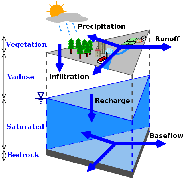
Figure 3 depicts the geometric structure of the discrete cells in SHUD. The watershed domain is discretized using an irregular unstructured triangular network (Delaunay triangles) generated with imposed spatial constraints by triangle (Shewchuk, 1996). Non-Delaunay triangulations are also permitted, so any GIS software and advanced programming language (R, MATLAB, and Python) could potentially generate the triangular domain. A prismatic control volume is formed by the vertical extension of the Delaunay triangles to produce three layers: land surface layer, unsaturated zone, and groundwater layer. The modeler is responsible for defining the aquifer depth (from the land surface to the impervious bedrock) based on measurements or terrestrial characteristics. The thickness of the unsaturated zone (D_us) is determined by the difference between the land surface elevation (z_sf) and groundwater table (z_gw) above datum, i.e., $D_{\mathrm{us}}=z_{\mathrm{sf}}-z_{\mathrm{gw}}$. When the groundwater table reaches the land surface (z_gw>z_sf), the thickness of unsaturated zone →0.

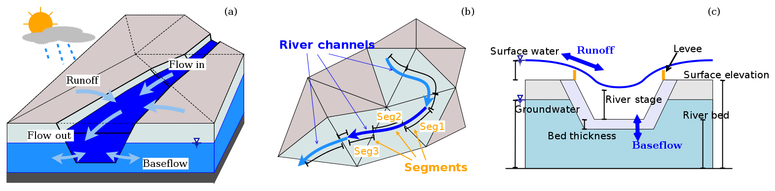
Figure 4 A depiction of the interaction between cells and the river network in SHUD showing (a) water balance in river channels, (b) the topologic relationship between river channels and hillslope cells, and (c) water fluxes between river segments and hillslope cells.

Figure 4 depicts the exchange of water between the rivers and hillslope cells. Within each river channel, there are two longitudinal fluxes and two lateral fluxes: upstream (Q_up), downstream (Q_dn), overland (Q_sf), and groundwater (Q_sub).

The hydrologic model uses the method of moments to reduce the partial differential equations (PDEs) into ordinary differential equations (ODEs) and solve the ODE system using a globally implicit numerical solver. The state variables include water height on the land surface (Y_sf), soil moisture storage (Y_us), groundwater depth (Y_gw), and river stage (Y_riv). The initial value problem for these ODEs is formulated as

$${\displaystyle \frac{\mathrm{d}\mathit{Y}}{\mathrm{d}t}}=f(t,\mathit{Y}),\mathit{Y}\left(t_{\mathrm{0}}\right)={\mathit{Y}}_{\mathrm{0}},$$

where the discrete state vector is denoted by Y,

$$\mathit{Y}=\left(\begin{array}{l}{\mathit{Y}}_{\mathrm{sf}}\\ {\mathit{Y}}_{\mathrm{us}}\\ {\mathit{Y}}_{\mathrm{gw}}\\ {\mathit{Y}}_{\mathrm{riv}}\end{array}\right).$$

Y₀ contains the initial conditions, and f(t,Y) denotes the equations governing the hydrologic flow, which are described in this section.

The system of ODEs describing the hydrologic processes are fully coupled and solved simultaneously at each time step ($\mathrm{\Delta }t=t_n-t_{n-\mathrm{1}}$) using CVODE, a stiff solver based on Newton–Krylov iteration (Hindmarsh et al., 2019). In brief, the CVODE solver calculates Y(t_n), given Y(t_n−1) and $\frac{\mathrm{d}\mathit{Y}}{\mathrm{d}t}{\mathrm{|}}_{t_{n-\mathrm{1}}}$. The technical description of the CVODE solver can be found in the literature (Hindmarsh et al., 2019, 2005; Cohen and Hindmarsh, 1996). The governing equations in SHUD are provided in Table 1.

Table 1 The governing equations in the SHUD model.

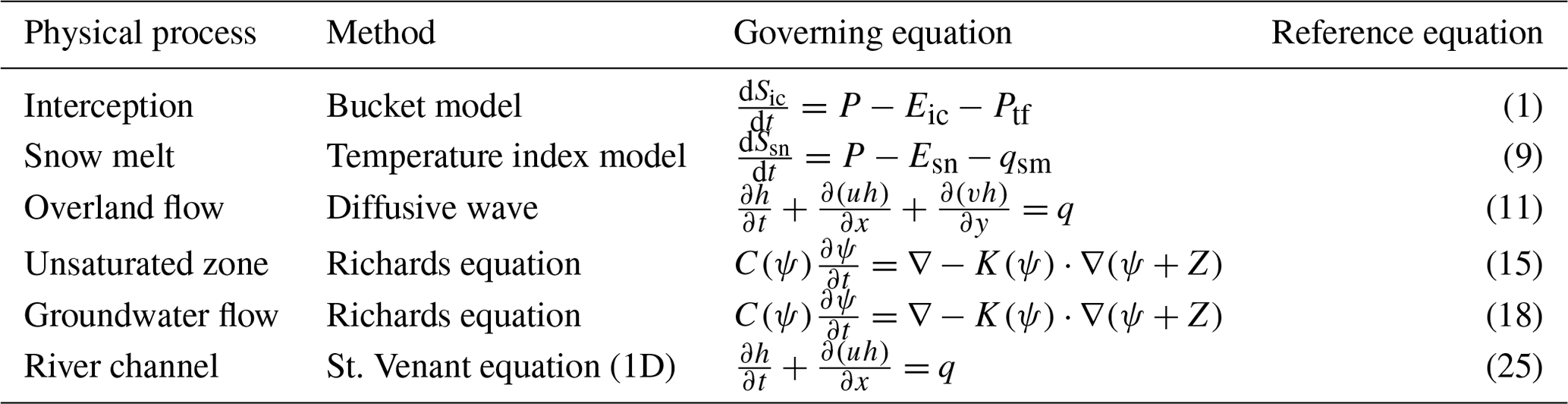
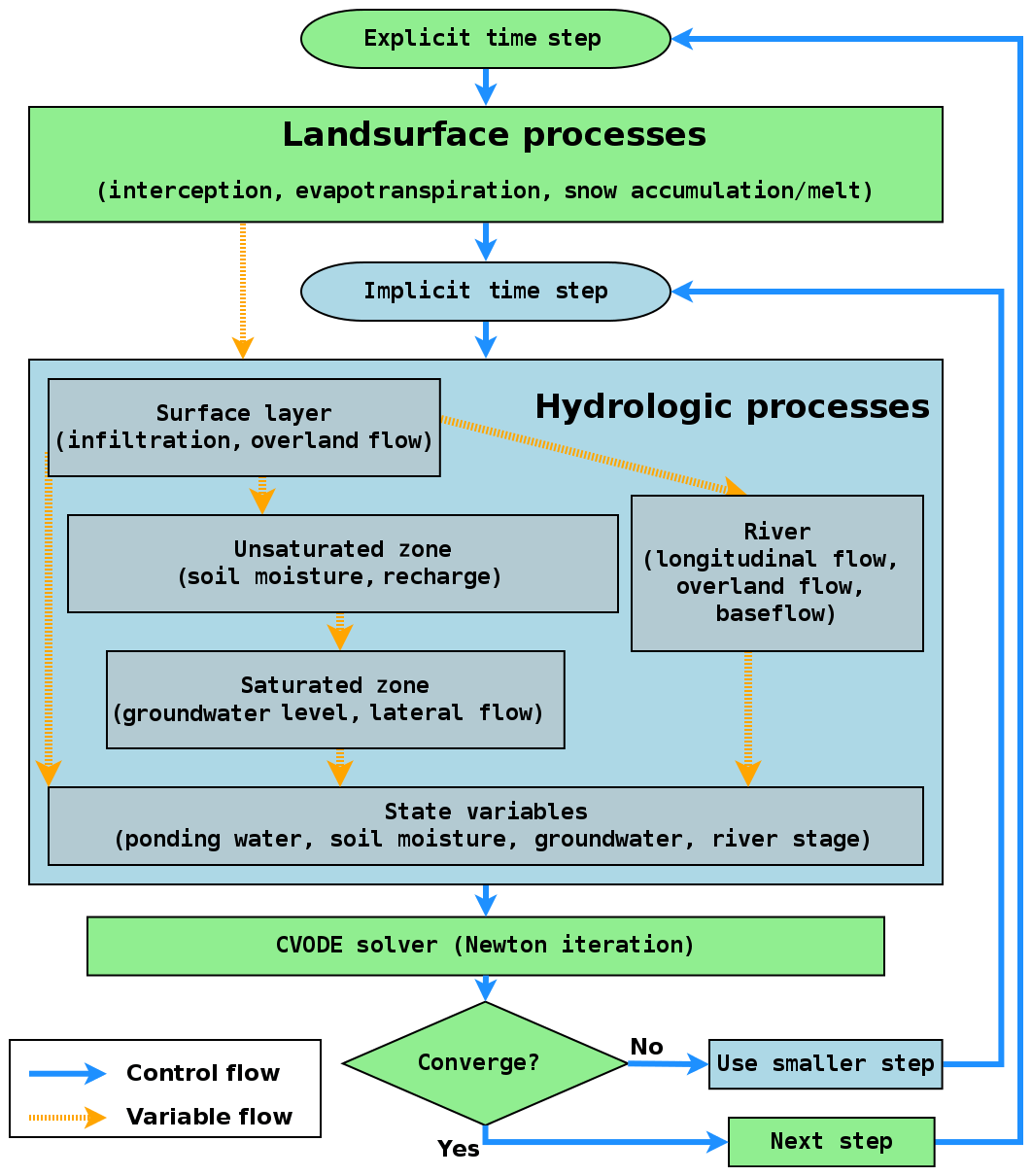
Figure 5 The flowchart demonstrates calculation of variables and time step control in the SHUD model. The hydrologic processes are simulated in each finite volume cell, then the state variables (Y) are passed to the CVODE solver.

Figure 5 depicts the workflow within the SHUD model. The explicit model time step (MTS) $\mathrm{\Delta }t=t_n-t_{n-\mathrm{1}}$ is user specified, typically varying from 1 min to 1 h. Within the MTS, the relevant gradient law determines the fluxes and hence all state values.

The fluxes of ET and interception change relatively slowly within short periods (such as 1 h) so that full coupling of ET with soil water is not necessary for this model. Instead, the interception, ET, and snow calculations are solved explicitly at the MTS, while the calculation of Y_sf, Y_us, Y_gw, and Y_riv uses the implicit time step (ITS).

The CVODE solver determines the ITS automatically based on both the specified tolerances and the error function of Y and dY. The initial ITS equates to the explicit MTS. Within the ITS, dYs is calculated based on Y from the last MTS. If the CVODE solver converges with the current value of the ITS, it returns the updated Y. Otherwise, a convergence failure occurs that forces an ITS reduction.

The mathematical model underlying SHUD consists of five components: vegetation and evapotranspiration, land surface, unsaturated layer, saturated layer, and river channel. These are described in the following subsections.

2.2.1 Vegetation and evapotranspiration

Interception refers to the direct water loss of precipitation when vegetation cover exists and is treated as a simple storage bucket – namely, precipitation cannot reach the land surface until the interception storage capacity is satisfied. The capacity of this storage is the maximum interception volume, which is a function of the vegetation leaf area index (LAI) and satisfies equation $S_{\mathrm{ic}}^{*}=C_{\mathrm{ic}}\mathrm{LAI}$, where LAI represents the coverage of vegetation canopy over the land area (area of leaves over the area of land, in m² m⁻²), and C_ic is interception coefficient (in m). The default C_ic is taken to be 0.2 kg m⁻² as suggested in Dickinson (1984).

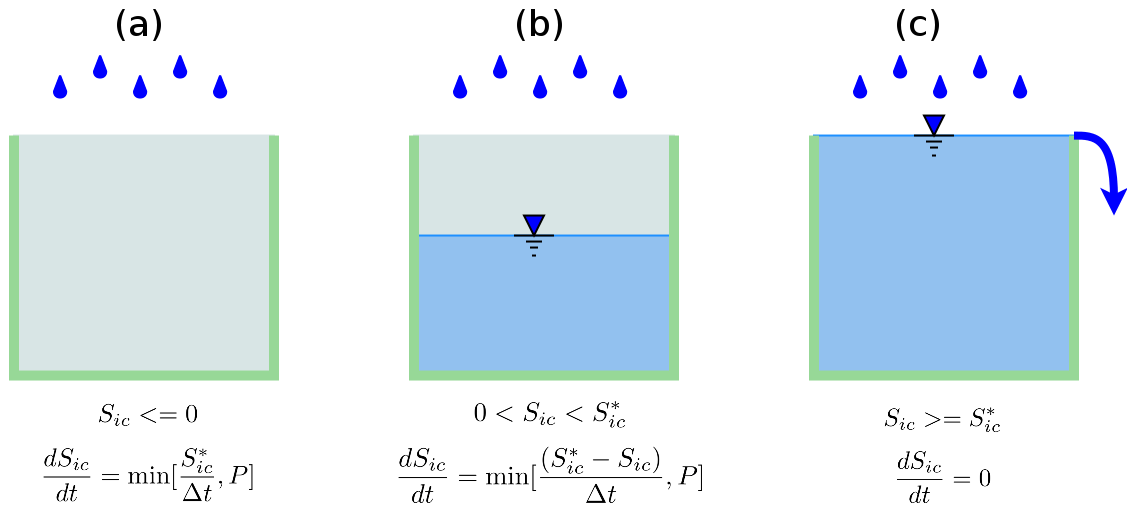
Figure 6 The three conditions for the interception calculation within the imaginary canopy bucket. The throughfall or excess precipitation after interception produces the water gain on the land surface.

The interception is equal to the deficit of interception – the difference between interception capacity ($S_{\mathrm{ic}}^{*}$) and existing interception storage (S_ic). If precipitation is less than the deficit, interception is equal to the precipitation rate (see Fig. 6).

$$\begin{array}{}\text{(1)}& {\displaystyle \frac{\mathrm{d}{S}_{\mathrm{ic}}}{\mathrm{d}t}}=q_{\mathrm{ic}}-E_{\mathrm{ic}}\text{(2)}& {\displaystyle }{q}_{\mathrm{ic}}=\left\{\begin{array}{lrr}min\left[\frac{S_{\mathrm{ic}}^{*}}{\mathrm{\Delta }t},P\right]& & S_{\mathrm{ic}}<=\mathrm{0}\\ min\left[\frac{(S_{\mathrm{ic}}^{*}-S_{\mathrm{ic}})}{\mathrm{\Delta }t},P\right]& & \mathrm{0}<S_{\mathrm{ic}}<S_{\mathrm{ic}}^{*}\\ \mathrm{0}& & S_{\mathrm{ic}}\mathit{>=}{S}_{\mathrm{ic}}^{*}\end{array}\right.\end{array}$$

Potential evapotranspiration (PET) is the quantity of water that would evaporate and transpire from an ideal surface if extensive free water was available to meet the demand (Maidment, 1993; Kirkham, 2014). As such, PET is a practical and rapid estimation of water flux from land to atmosphere. The PET (E₀) is governed by Penman–Monteith equation (Penman, 1948):

$$\begin{array}{}\text{(3)}& E_{\mathrm{0}}={\displaystyle \frac{\mathrm{1}}{\mathit{\lambda }}}{\displaystyle \frac{\mathrm{\Delta }\left(R_{\mathrm{n}}-G\right)+{\mathit{\rho }}_{\mathrm{a}}{c}_p\frac{\left(e_{\mathrm{s}}-e_{\mathrm{a}}\right)}{r_{\mathrm{a}}}}{\mathrm{\Delta }+\mathit{\gamma }\left(\mathrm{1}+\frac{r_{\mathrm{s}}}{r_{\mathrm{a}}}\right)}}.\end{array}$$

Here we do not elaborate on this equation, as it is common among different hydrologic models (Allen, 1998; Maidment, 1993). At each ET step, the model calculates PET in terms of the prescribed forcing data. PET values are conditioned on the parameters from various land cover types, including factors for albedo, LAI, and roughness length.

The total actual evapotranspiration (AET) consists of three parts: evaporation from interception (E_c), transpiration from vegetation canopy (E_t), and direct evaporation of soil (E_s). The calculation of AET for these three components follows from the equations below:

$$\begin{array}{}\text{(4)}& {\displaystyle }& {\displaystyle }{E}_{\mathrm{c}}=max[S_{\mathrm{ic}}/\mathrm{\Delta }t,E_{\mathrm{0}}],\text{(5)}& {\displaystyle }& {\displaystyle }{E}_{\mathrm{s}}=E_{\mathrm{0}}{\mathit{\beta }}_{\mathrm{s}}(\mathrm{1}-{\mathit{\alpha }}_{\mathrm{imp}})(\mathrm{1}-{\mathit{\alpha }}_{\mathrm{veg}}),\text{(6)}& {\displaystyle }& {\displaystyle }{E}_{\mathrm{t}}=E_{\mathrm{0}}{\mathit{\beta }}_{\mathrm{s}}(\mathrm{1}-{\mathit{\alpha }}_{\mathrm{imp}}){\mathit{\alpha }}_{\mathrm{veg}},\text{(7)}& {\displaystyle }& {\displaystyle }{\mathit{\beta }}_{\mathrm{s}}={\displaystyle \frac{\mathit{\theta }-{\mathit{\theta }}_{\mathrm{r}}}{{\mathit{\theta }}_{\mathrm{fc}}-{\mathit{\theta }}_{\mathrm{r}}}}.\end{array}$$

Here, E_c is controlled by PET from interception storage. Both E_s and E_t are affected by soil water stress (β_s) and impervious area fraction (α_imp). Impervious area is also considered a barrier of evapotranspiration in the model. E_s is referred to as the demand water evaporation from soil and emerges from two sources, namely the evaporation from ponding water (E_sp) and evaporation from soil moisture (E_sm), $E_{\mathrm{s}}=E_{\mathrm{sp}}+E_{\mathrm{sm}}$. Ponded water has higher priority to evaporate and direct evaporation only uses the water in the surface when ponding water is able to meet the E_s demand, i.e., $y_{\mathrm{sf}}/\mathrm{\Delta }t>E_{\mathrm{s}}$. When ponding water is insufficient to meet E_s, soil water balances the difference between demand and available water in the surface; when ponding water does not exist, direct evaporation extracts water from the soil profile ($E_{\mathrm{sm}}=E_{\mathrm{s}},E_{\mathrm{sp}}=\mathrm{0}$):

$$\begin{array}{}\text{(8)}& \left\{\begin{array}{llr}{E}_{\mathrm{sp}}=E_{\mathrm{s}},& E_{\mathrm{sm}}=\mathrm{0},& y_{\mathrm{sf}}>E_{\mathrm{s}}\times \mathrm{\Delta }t,\\ E_{\mathrm{sp}}=y_{\mathrm{sf}}/\mathrm{d}t,& E_{\mathrm{sm}}=E_{\mathrm{s}}-E_{\mathrm{sp}},& y_{\mathrm{sf}}<E_{\mathrm{s}}\times \mathrm{\Delta }t,\\ E_{\mathrm{sp}}=\mathrm{0},& E_{\mathrm{sm}}=E_{\mathrm{s}},& y_{\mathrm{sf}}<=\mathrm{0}.\end{array}\right.\end{array}$$

Transpiration also has two potential sources: soil moisture and groundwater from the groundwater table and root depth for the land-use class. Once the groundwater table is higher than the root zone depth, vegetation uses groundwater, and soil moisture stress for transpiration is equal to one (β_s=1). Water balance associated with snow accumulation is quantified via

$$\begin{array}{}\text{(9)}& {\displaystyle }& {\displaystyle \frac{\mathrm{d}{S}_{\mathrm{sn}}}{\mathrm{d}t}}=P_{\mathrm{sn}}-q_{\mathrm{sn}},\text{(10)}& {\displaystyle }& {\displaystyle }{q}_{\mathrm{sn}}=(T-T_{\mathrm{0}})\times m_{\mathrm{f}}.\end{array}$$

Snow melt rate is determined by the snow melting factor (m_f), air temperature (T), and temperature threshold (T₀) at which snow melt occurs. This formulation is often referred to as the degree-day method, in which the values of the snow melting factor and temperature threshold are empirical (Maidment, 1993; Beven, 2012). The water from snowmelt is considered as a direct water contribution to the land surface.

2.2.2 Water on the land surface

Water balance on the land surface is given by

$$\begin{array}{}\text{(11)}& {\displaystyle }& {\displaystyle \frac{\mathrm{d}{y}_{\mathrm{sf}}}{\mathrm{d}t}}=P_{\mathrm{n}}-E_{\mathrm{sp}}-q_{\mathrm{i}}-\sum _{j=\mathrm{1}}^{\mathrm{3}}{\displaystyle \frac{Q_{\mathrm{s}}^j}{A_{\mathrm{c}}}},\text{(12)}& {\displaystyle }& {\displaystyle }{P}_{\mathrm{n}}=P-S_{\mathrm{ic}}+q_{\mathrm{sn}},\text{(13)}& {\displaystyle }& {\displaystyle }{Q}_{\mathrm{s}}^j={\displaystyle \frac{L_j}{n}}{\stackrel{\mathrm{‾}}{y_{\mathrm{sf}}}}^{\frac{\mathrm{5}}{\mathrm{3}}}{s}_{\mathrm{0}}^{\frac{\mathrm{1}}{\mathrm{2}}}.\end{array}$$

The water balance of net precipitation (P_n), infiltration (q_i), evaporation from the ponding layer (E_sp), and horizontal overland flow (Q_j) determine the storage of water on the land surface. Net precipitation (P_n) is the total residual water after adjusting for rainfall/snow interception and snowmelt. The overland flow $Q_{\mathrm{s}}^j$ in direction j is calculated with Manning's equation (13). Here $\stackrel{\mathrm{‾}}{y_{\mathrm{sf}}}$ is effective water height, determined by the gradient between two cells,

$$\begin{array}{}\text{(14)}& \stackrel{\mathrm{‾}}{y_{\mathrm{sf}}}=\left\{\begin{array}{lr}{y}_{\mathrm{sf}}& z_{\mathrm{sf}}+y_{\mathrm{sf}}\mathit{>=}{z}_{\mathrm{sf}}^j+y_{\mathrm{sf}}^j\\ y_{\mathrm{sf}}^j& z_{\mathrm{sf}}+y_{\mathrm{sf}}<z_{\mathrm{sf}}^j+y_{\mathrm{sf}}^j.\end{array}\right.\end{array}$$

Infiltration is estimated using Richards equation:

$$\begin{array}{ll}{\displaystyle }& {\displaystyle }{q}_{\mathrm{i}}=K_{\mathrm{ei}}\left(\mathrm{\Theta }\right)\left(\mathrm{1}+{\displaystyle \frac{y_{\mathrm{s}}}{D_{\inf }}}\right)\\ {\displaystyle }& {\displaystyle }{K}_{\mathrm{ei}}\left(\mathrm{\Theta }\right)=\left\{\begin{array}{lr}{K}_r\left(\mathrm{\Theta }\right)k_x(\mathrm{1}-{\mathit{\alpha }}_{\mathrm{h}})+{\mathit{\alpha }}_{\mathrm{h}}{k}_{\mathrm{m}}\mathrm{\Theta }& y_{\mathrm{s}}/\mathrm{\Delta }t\mathit{>=}{K}_{max}\\ K_r\left(\mathrm{\Theta }\right)k_x(\mathrm{1}-{\mathit{\alpha }}_{\mathrm{h}})& y_{\mathrm{s}}/\mathrm{\Delta }t<K_{max}\end{array}\right.\\ {\displaystyle }& {\displaystyle }{K}_{\mathrm{r}}\left(\mathrm{\Theta }\right)={\mathrm{\Theta }}^{\frac{\mathrm{1}}{\mathrm{2}}}{\left(-\mathrm{1}+{\left(\mathrm{1}-{\mathrm{\Theta }}^{\frac{\mathit{\beta }}{\mathit{\beta }-\mathrm{1}}}\right)}^{\frac{\mathit{\beta }-\mathrm{1}}{\mathit{\beta }}}\right)}^{\mathrm{2}}\\ {\displaystyle }& {\displaystyle }{K}_{max}=k_x(\mathrm{1}-{\mathit{\alpha }}_{\mathrm{h}})+{\mathit{\alpha }}_{\mathrm{h}}{k}_{\mathrm{m}}.\end{array}$$

The infiltration rate is a function of soil saturation ratio (Θ), soil properties (k_x, k_m α, β, and α_h), and ponding water height (existing ponding water plus precipitation/irrigation). Infiltration occurs in the top soil layer (D_inf), and the infiltration rate results from the ponding water height and soil moisture. The default value of D_inf is 10 cm, which is adjustable in calibration files. The application rate y_s∕Δt combines ponding water, irrigation, and precipitation together, and that determines the hydraulic gradient applied on the top soil layer. Finally, K_max is the infiltration capacity determined by both soil matrix and macropore characteristics. When application rate is less than the maximum infiltration capacity, the infiltration is controlled by soil matrix flow; when application rate is larger than K_max, effective conductivity is a function of the soil matrix and macropores (Chen and Wagenet, 1992). The infiltration equation takes the macropore effect into account, so the algorithm allows faster infiltration under heavy rainfall events and enables the soil to hold water for vegetation under dry conditions.

2.2.3 Unsaturated zone

As discussed above, the horizontal flow in the vadose zone is neglected compared to the dominant vertical flow. There are three processes controlling the water in vadose zone: infiltration (q_i), ET in soil moisture (E_sm), and recharge to groundwater (q_r). The calculation of infiltration and ET is explained in the previous subsection. Recharge to groundwater is calculated with Eq. (16). The soil moisture content to field capacity controls the recharge rate.

$$\begin{array}{}\text{(15)}& {\displaystyle }& {\displaystyle }{s}_{\mathrm{y}}{\displaystyle \frac{\mathrm{d}{y}_{\mathrm{us}}}{\mathrm{d}t}}=q_{\mathrm{i}}-q_{\mathrm{r}}-E_{\mathrm{sm}},\text{(16)}& {\displaystyle }& {\displaystyle }{q}_{\mathrm{r}}=K_{\mathrm{er}}\left({\displaystyle \frac{\mathit{\theta }-{\mathit{\theta }}_{\mathrm{r}}}{{\mathit{\theta }}_{\mathrm{fc}}-{\mathit{\theta }}_{\mathrm{r}}}}\right)\text{(17)}& {\displaystyle }& {\displaystyle }{K}_{\mathrm{er}}={\displaystyle \frac{D_{\mathrm{us}}+y_{\mathrm{gw}}}{D_{\mathrm{us}}/k_x+y_{\mathrm{gw}}/k_{\mathrm{v}}}}\end{array}$$

Because of the simplifications required for the two-layer description of the vertical aquifer profile, SHUD uses the relationship between soil moisture and field capacity as the gradient to drive the recharge instead of the hydraulic gradient. K_er is the effective conductivity for recharge and is equal to the arithmetic mean of the conductivity of the unsaturated zone and saturated zone.

When the bottom of the vegetation root zone is below the groundwater table, then E_tg>0 and vegetation extracts water from the saturated zone. Otherwise E_tg=0, meaning that transpiration uses soil moisture. When ponding water exists on the land surface, direct evaporation extracts water from ponding water first; when ponding water is depleted via evaporation, then the remainder of evaporation (E_sm) uses water from soil moisture based on the water stress.

2.2.4 Groundwater

The water balance of groundwater is controlled by Eq. (18).

$$\begin{array}{}\text{(18)}& {\displaystyle }& {\displaystyle }{s}_{\mathrm{y}}{\displaystyle \frac{\mathrm{d}{y}_{\mathrm{gw}}}{\mathrm{d}t}}=q_{\mathrm{r}}-E_{\mathrm{tg}}-\sum _{j=\mathrm{1}}^{\mathrm{3}}{\displaystyle \frac{Q_{\mathrm{g}}^j}{A_{\mathrm{c}}}},\text{(19)}& {\displaystyle }& {\displaystyle }{Q}_{\mathrm{g}}^j=\stackrel{\mathrm{‾}}{K}\cdot {\displaystyle \frac{\left(y_{\mathrm{gw}}+z_{\mathrm{b}}\right)-\left(y_{\mathrm{gw}}^j+z_{\mathrm{b}}^j\right)}{d_j}}\cdot \left(L_j\stackrel{\mathrm{‾}}{y_{\mathrm{gw}}}\right),\text{(20)}& {\displaystyle }& {\displaystyle }\stackrel{\mathrm{‾}}{K}=\left(K_{\mathrm{eg}}+K_{\mathrm{cg}}^j\right)\cdot \mathrm{0.5}\end{array}$$

The calculation of horizontal groundwater flow uses the Boussinesq equation. When the bottom of the root zone is lower than the groundwater table, then E_t>0, otherwise, E_t=0.

The horizontal groundwater flux $Q_{\mathrm{g}}^j$ is determined by the Darcy equation and Dupuit–Forchheimer assumption. Above z_b is the elevation of impervious bedrock; $z_{\mathrm{b}}^j$ is the bedrock elevation of its jth neighbor cell, and d_j is distance between the centroids of two adjacent cells, so the gradient between the two cells is $\left[\left(y_{\mathrm{gw}}+z_{\mathrm{b}}\right)-\left(y_{\mathrm{gw}}^j+z_{\mathrm{b}}^j\right)\right]d_j^{-\mathrm{1}}$. The effective conductivity for the groundwater flow is the mean value of the effective horizontal conductivity over the two cells. The cross-sectional area along the groundwater flux is equal to $L_j\times \stackrel{\mathrm{‾}}{y_{\mathrm{gw}}}$.

In Eq. (20), the effective horizontal conductivity (K_eg) is a function of the groundwater table and characteristics of the macropores. The calculation of effective horizontal conductivity of each cell is given by

$$\begin{array}{}\text{(21)}& {\displaystyle }& {\displaystyle }{K}_{\mathrm{eg}}=\left\{\begin{array}{lr}{k}_{\mathrm{g}},& z_{\mathrm{m}}>z_{\mathrm{gw}},\\ \frac{z_{\mathrm{gw}}-z_{\mathrm{m}}}{y_{\mathrm{gw}}}(k_{\mathrm{m}}{\mathit{\alpha }}_{\mathrm{v}}+(\mathrm{1}-{\mathit{\alpha }}_{\mathrm{v}}\left)k_{\mathrm{g}}\right)+k_{\mathrm{g}},& z_{\mathrm{m}}<z_{\mathrm{gw}},\end{array}\right.\text{(22)}& {\displaystyle }& {\displaystyle }{z}_{\mathrm{gw}}=y_{\mathrm{gw}}+z_{\mathrm{cb}},\end{array}$$

where k_g and k_m are the saturated hydraulic conductivity of soil matrix and macropores, z_m, z_gw, and z_cb are elevations of macropore, groundwater table, and bedrock, and α_v is the vertical areal macropore fraction (in m² m⁻²).

The effective horizontal conductivity captures the effect of spatially varying conductivity on the saturated flow when the groundwater level rises (Jiang et al., 2009; Bobo et al., 2012; Chen et al., 2018; Cheema, 2015; Taylor, 1960; Lin et al., 2007). Figure 7 reveals the effective horizontal conductivity changes along with different groundwater levels. When the groundwater table is below the level of the macropores, K_eg is equal to the saturated conductivity. When the groundwater level is above the macropore level, the effective conductivity increases with the groundwater level, taking into consideration the conductivity and area fraction of macropores in the soil profile. The effective conductivity reaches its maximum value once the groundwater table level reaches the land surface.

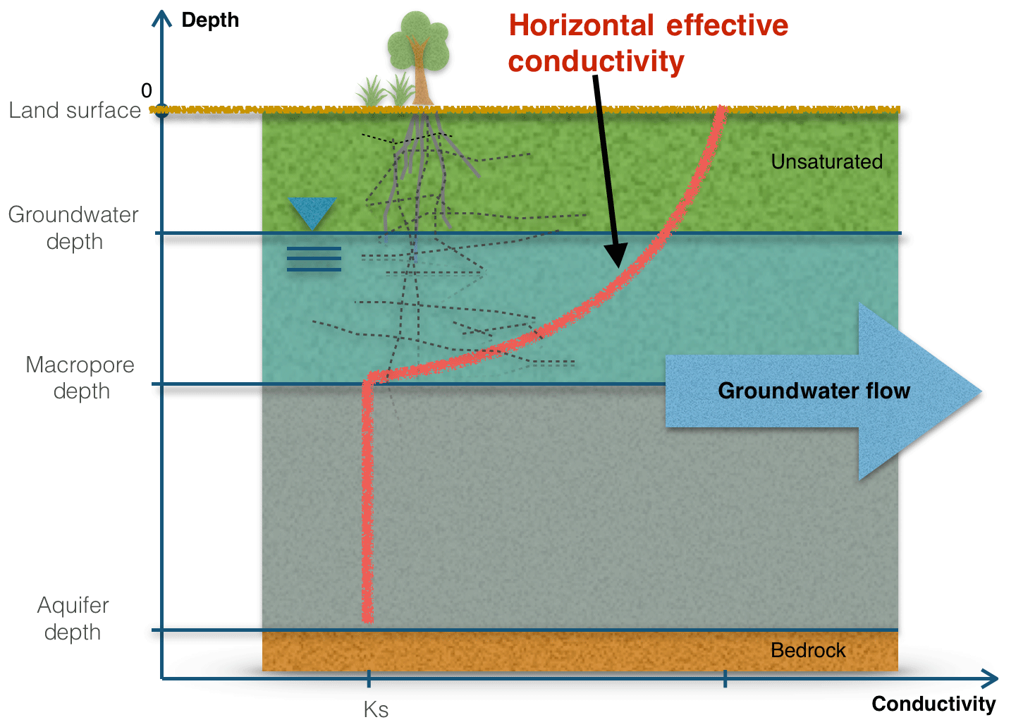
Figure 7 Effective conductivity for horizontal groundwater flow changes along the changing groundwater level. When the groundwater level is higher than macropore depth, groundwater flow increases due to the contribution of horizontal macropores.

2.2.5 Water in streams

The water balance in river channels is described by

$$\begin{array}{}\text{(23)}& {\displaystyle \frac{\mathrm{d}{y}_{\mathrm{riv}}}{\mathrm{d}t}}={\displaystyle \frac{\mathrm{1}}{A_{\mathrm{r}}}}\left(\sum _{j=\mathrm{1}}^{j=N_{\mathrm{c}}}{Q}_{\mathrm{sr}}^j+\sum _{j=\mathrm{1}}^{j=N_{\mathrm{c}}}{Q}_{\mathrm{gr}}^j+\sum _{j=\mathrm{1}}^{j=N_{\mathrm{u}}}{Q}_{\mathrm{up}}^j+Q_{\mathrm{dn}}\right).\end{array}$$

The mass balance in each river channel consists of four parts: $Q_{\mathrm{s}}^j$, the overland flow from cells (1 to N_c cells) that intersect with the river channel; $Q_{\mathrm{g}}^j$, the lateral groundwater flux from intersection with the jth cell; $Q_{\mathrm{up}}^j$, the longitudinal flow from upstream channels; and Q_dn, the flux to the downstream channel. N_u is the number of upstream channels; in the model, the number of upstream channels is nonnegative, but only one downstream channel is permitted. SHUD assumes river channels can converge to a single downstream channel. The convergence rule does not affect the topological relationship between river channels and cells.

The topological relationship between cells and river channels is shown in Fig. 4b. As depicted, the river consists of a series of river reaches which intersect prismatic elements. A single reach is a sorted collection of multiple river segments, while each segment lies within hillslope cells. Surface and groundwater exchanges occur between each segment and the underlying cell. The sum of overland flow from multiple cells contributes to the net storage in a river reach.

The downstream channel flux Q_dn is based on the 1-D diffusive wave equation that is simplified as Manning's equation for open channel:

$$\begin{array}{}\text{(24)}& {\displaystyle }{Q}_{\mathrm{dn}}={\displaystyle \frac{A_{\mathrm{cs}}}{\stackrel{\mathrm{‾}}{n}}}{\left({\displaystyle \frac{A_{\mathrm{cs}}}{\stackrel{\mathrm{‾}}{P}}}\right)}^{\frac{\mathrm{2}}{\mathrm{3}}}{\stackrel{\mathrm{‾}}{s_{\mathrm{0}}}}^{\frac{\mathrm{1}}{\mathrm{2}}},\end{array}$$

where A_cs is the cross-section area of the river reach, and $\stackrel{\mathrm{‾}}{P}$ and $\stackrel{\mathrm{‾}}{s_{\mathrm{0}}}$ are average wet perimeter and average slope of a river reach and its downstream reach.

The upstream flux Q_up is equal to the sum of Q_dn from the multiple upstream reaches. The water balance equation in the river channel neglects evaporation and precipitation because the area of open water in the watershed is relatively small, and the area of open water is already included in pre-computation for the cells. Therefore, the channel routing represents the water exchange between the river and hillslope and takes the overland flow and baseflow into account.

The overland flow between river segment and associated hillslope cell (Q_sr) is calculated as follows:

$$\begin{array}{}\text{(25)}& {\displaystyle }& {\displaystyle }{Q}_{\mathrm{sr}}=L_{\mathrm{s}}{C}_{\mathrm{w}}{b}_{\mathrm{s}}\sqrt{\mathrm{2}g\left|b_{\mathrm{s}}\right|},\text{(26)}& {\displaystyle }& {\displaystyle }{H}_{\mathrm{riv}}=y_{\mathrm{riv}}+z_{\mathrm{rb}},\text{(27)}& {\displaystyle }& {\displaystyle }{H}_{\mathrm{csf}}=y_{\mathrm{sf}}+z_{\mathrm{cs}},\text{(28)}& {\displaystyle }& {\displaystyle }{b}_{\mathrm{s}}=\left\{\begin{array}{lr}{H}_{\mathrm{riv}}-H_{\mathrm{csf}},& H_{\mathrm{riv}}>z_{\mathrm{bank}}\text{and}{H}_{\mathrm{csf}}>z_{\mathrm{bank}},\\ H_{\mathrm{riv}}-z_{\mathrm{bank}},& H_{\mathrm{riv}}>z_{\mathrm{bank}}\text{and}{H}_{\mathrm{csf}}<z_{\mathrm{bank}},\\ H_{\mathrm{csf}}-z_{\mathrm{bank}},& H_{\mathrm{riv}}<z_{\mathrm{bank}}\text{and}{H}_{\mathrm{csf}}>z_{\mathrm{bank}}.\end{array}\right.\end{array}$$

Here z_bank is the elevation of riverbank or levee (Fig. 4c), implying that the relative height of the land surface or river stage controls the direction of water exchange between the land surface and river segment.

The groundwater exchange between river segment and hillslope cell is described by Q_gr, which is calculated as

$$\begin{array}{}\text{(29)}& {\displaystyle }& {\displaystyle }{Q}_{\mathrm{gr}}=L_{\mathrm{s}}{b}_{\mathrm{g}}{K}_{\mathrm{gr}}{\displaystyle \frac{H_{\mathrm{riv}}-H_{\mathrm{cgw}}}{d_{\mathrm{rb}}}},\text{(30)}& {\displaystyle }& {\displaystyle }{H}_{\mathrm{cgw}}=y_{\mathrm{gw}}+z_{\mathrm{cb}},\text{(31)}& {\displaystyle }& {\displaystyle }{b}_{\mathrm{g}}=\left\{\begin{array}{lrr}{y}_{\mathrm{riv}},& & H_{\mathrm{cgw}}<z_{\mathrm{rb}},\\ \frac{\mathrm{1}}{\mathrm{2}}\left(y_{\mathrm{riv}}+H_{\mathrm{cgw}}-z_{\mathrm{rb}}\right),& & H_{\mathrm{cgw}}>z_{\mathrm{rb}},\end{array}\right.\text{(32)}& {\displaystyle }& {\displaystyle }{K}_{\mathrm{gr}}={\displaystyle \frac{\mathrm{1}}{\mathrm{2}}}\left(k_{\mathrm{rb}}+K_{\mathrm{eg}}\right).\end{array}$$

3 Applications

In this section, we present the results of using SHUD for three applications: first, we use the V-catchment experiment (Shu, 2019e) to validate the calculation of overland flow and river routing in an idealized catchment; second, we use Vauclin's experiment (Vauclin et al., 1979) to assess the calculation of infiltration, unsaturated flow in the vadose zone and horizontal saturated flow; finally, we apply the model to a hydrologic simulation in the Cache Creek Watershed (Shu, 2019a), a headwater catchment in the Sacramento Watershed of northern California.

3.1 V-catchment

The V-catchment (VC) experiment is a standard test case for numerical hydrologic models to validate their performance for overland flow along a hillslope and in the presence of a river channel (Shen and Phanikumar, 2010). The VC domain consists of two inclined planes draining into a sloping channel (Fig. 8). Both hillslopes are 800 m×1000 m with Manning's roughness n=0.015. The river channel between the hillslopes is 20 m wide and 1000 m in length with n=0.15. The slope from the ridge to the river channel is 0.05 (in the x direction), and the longitudinal slope (in the y direction) is 0.02.

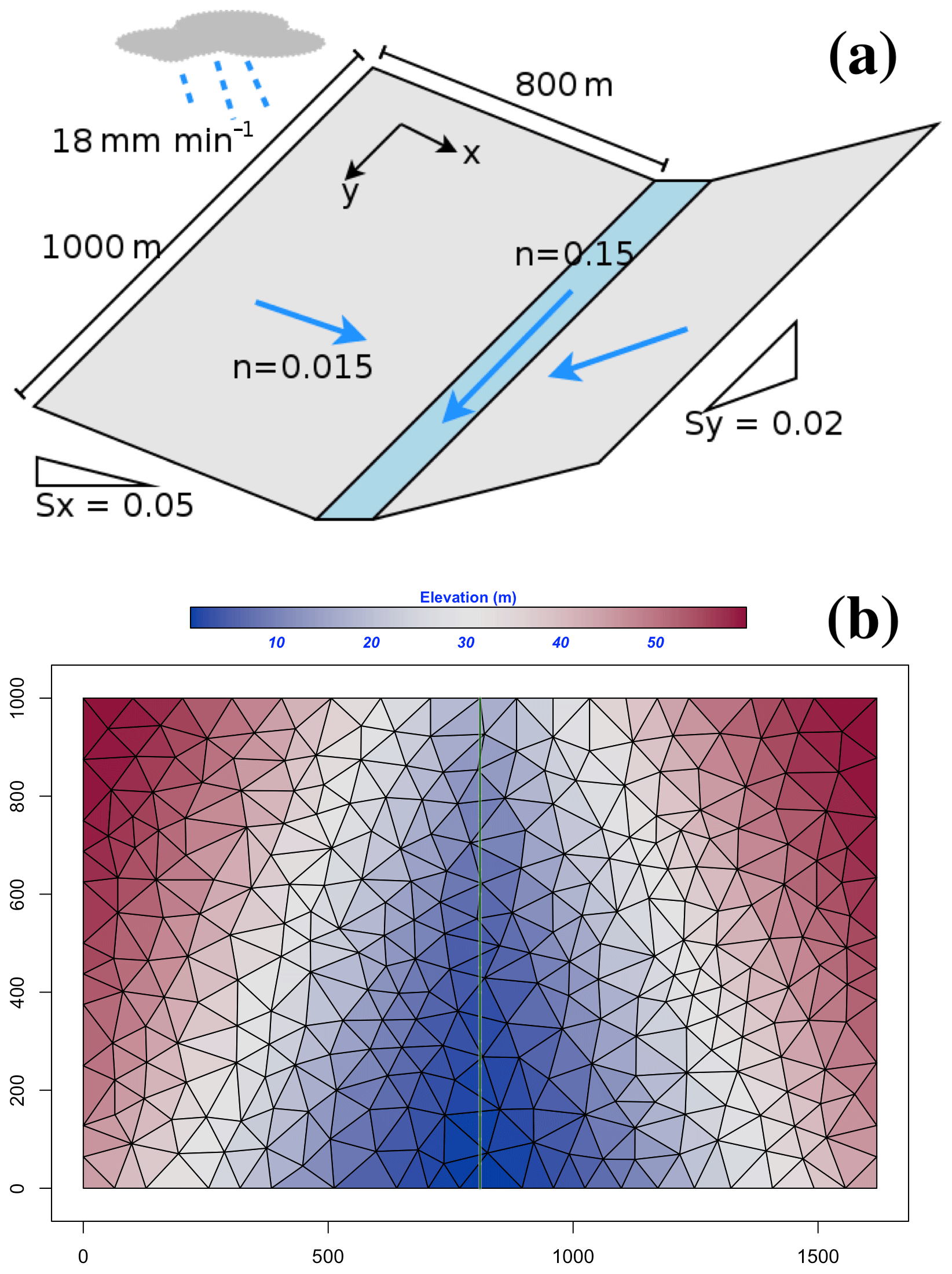
Figure 8 The tilted V-catchment: (a) basic structure of V-catchment; (b) the SHUD mesh used for the V-catchment with elevation colored.

Rainfall in the VC begins at time zero at a constant rate of 18 mm h⁻¹ and stops after 90 min, producing 27 mm of accumulated precipitation. Since this experiment excludes the evaporation and infiltration, the total outflow from lateral boundaries and the river outlet must be the same as the total precipitation (following conservation of mass).

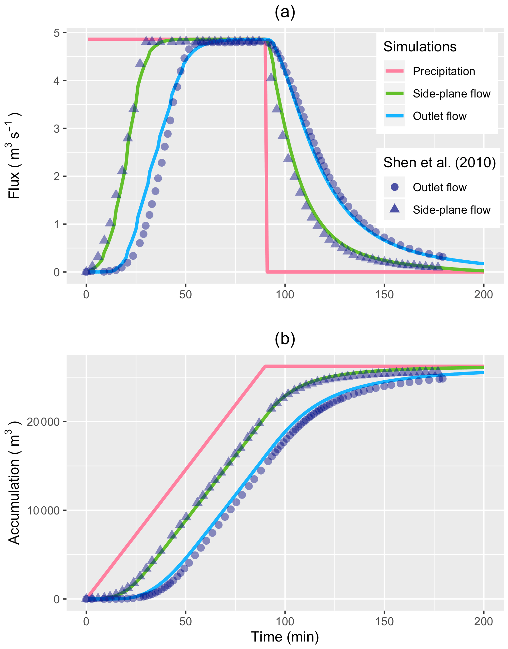
Figure 9 Comparison of overland flow and outflow at the outlet of the V-catchment from the SHUD modeling versus Shen and Phanikumar (2010). Panel (a) is volume fluxes, while (b) is accumulated water volume.

Figure 9 illustrates the discharge from the side plane to the river channel and at the river outlet. The specific discharge (the volume discharge divided by the total area of the catchment) increases with precipitation until it reaches the maximum discharge rate, which is equal to the precipitation rate. Discharges along lateral boundaries and from the river outlet reach the maximum discharge rate but at different times; namely, the discharge rate from the side plane reaches the maximum value earlier than in the river outlet. The dots are discharge digitalized from Shen and Phanikumar (2010) with WebPlotDigitizer (https://automeris.io/WebPlotDigitizer/, last access: 19 December 2019). The results suggest SHUD can correctly capture the processes in overland flow and channel routing, although flow from the river outlet occurs earlier than the prediction in Shen and Phanikumar (2010). Both the fluxes from side plane and outlet meet the maximum flow rate, which is the same magnitude of precipitation after a short period of rainfall. The flux rates start decreasing after precipitation stops. The accumulated volume of flux confirms the correct mass balance of both fluxes.

To verify correct performance of the numerical method, we calculate the bias of mass balance in the model and assess the differences among input, output, and storage change in the system (Eq. 35). For this simulation the bias ends up being ∼0.2 %.

$$\begin{array}{}\text{(33)}& {\displaystyle }& {\displaystyle }\mathrm{\Delta }S=P-Q-E\text{(34)}& {\displaystyle }& {\displaystyle }\widehat{\mathrm{\Delta }S}=\mathrm{\Delta }{S}_{\mathrm{ic}}+\mathrm{\Delta }{y}_{\mathrm{sf}}+\mathrm{\Delta }{y}_{\mathrm{us}}+\mathrm{\Delta }{y}_{\mathrm{gw}}+\mathrm{\Delta }{y}_{\mathrm{riv}}\text{(35)}& {\displaystyle }& {\displaystyle }\mathrm{Bias}=\left|{\displaystyle \frac{\widehat{\mathrm{\Delta }S}-\mathrm{\Delta }S}{\mathrm{\Delta }S}}\right|\times \mathrm{100}\mathit{\%}\end{array}$$

3.2 Vauclin's experiment

Vauclin's laboratory experiment (Vauclin et al., 1979) is to assess groundwater table change and soil moisture in the unsaturated layer under precipitation or irrigation. The experiment was conducted in a sandbox with dimensions of 3 m long ×2 m deep ×0.05 m wide (see Fig. 10). The box was full of uniform sand particles with measured hydraulic parameters: the saturated hydraulic conductivity was 35 cm h⁻¹, and porosity was 0.33 m³ m⁻³. The left and bottom of the sandbox were impervious layers, and the top and the right side were open. The hydraulic head was 0.65 m constantly on the right boundary. Constant irrigation (1.48 cm h⁻¹) was applied over the first 50 cm of the top left of the sandbox, while the rest of the top was covered to avoid water loss via evaporation.

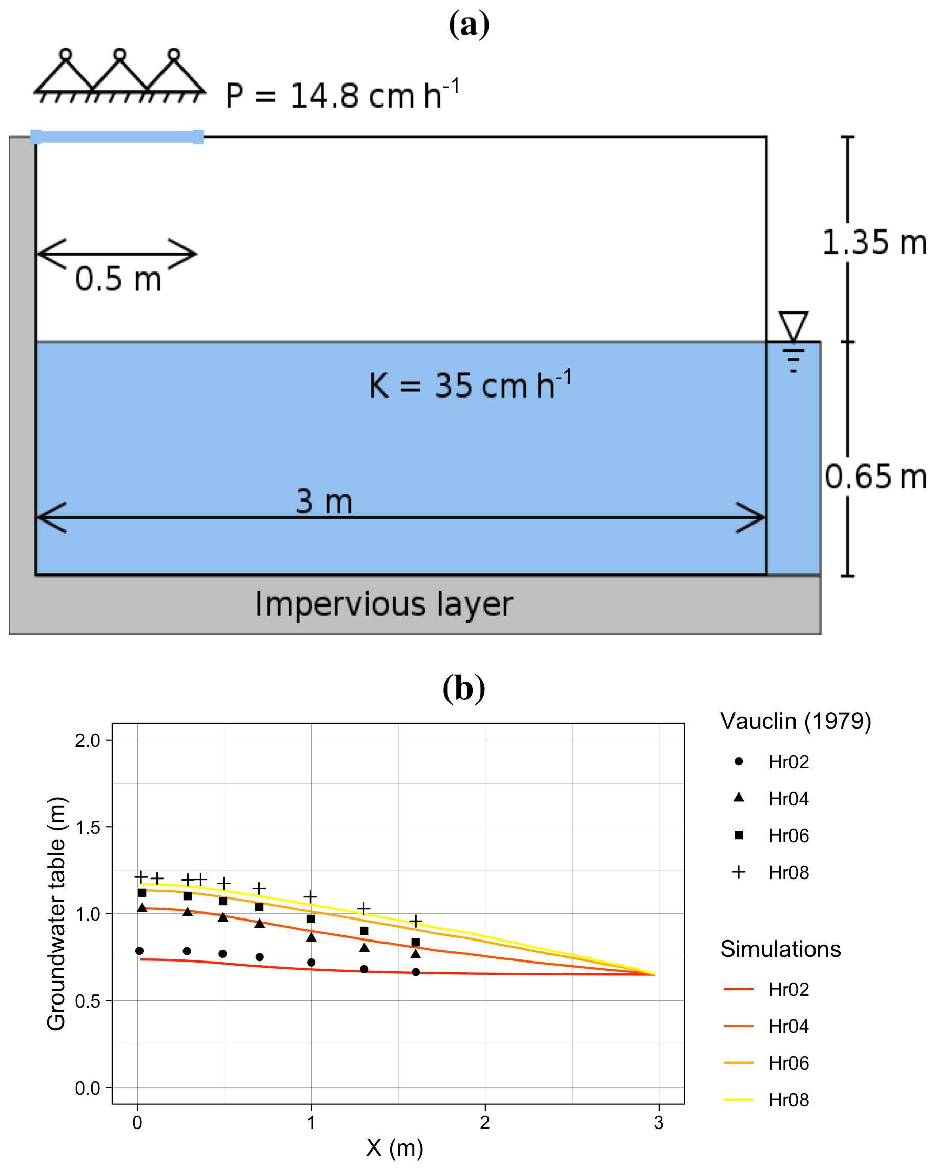
Figure 10 A schematic of (a) Vauclin's experiment and (b) a comparison of Vauclin's measurements versus simulated groundwater table change with SHUD.

The experiment's initial condition is an equilibrium water table with a uniform hydraulic head. Irrigation was initiated at t=0. The groundwater table was then measured at 2, 4, 6, and 8 h at several locations along the length of the box. (Vauclin et al., 1979) also uses a 2-D (vertical and horizontal) numeric model to simulate the soil moisture and groundwater table. The maximum bias between measurement and simulation was 0.52 m, according to the digitalized value of Vauclin et al., 1979, Fig. 10.

Besides the parameters specified in Vauclin et al. (1979), additional information is needed in the SHUD model, including the α and β in the van Genuchten equation and residual water content (θ_r). Therefore, we use a calibration tool to estimate the representative values of these parameters. The use of calibration in this simulation is reasonable because the model, inevitably, simplifies the real hydraulic processes. The calibration thus nudges the parameters to representative values that approach or fit the true natural processes. The calibrated values are θ_r=0.001 m³ m⁻³, α=0.3 ,and β=5.2. The simulated results in our modeling and literature (Vauclin et al., 1979; Shen and Phanikumar, 2010) show a modest error between the simulations and measurements.

This error is likely due to (1) the need for a detailed aquifer layer description of soil layers or (2) possible invalidity of the vertical and horizontal flow assumptions in the SHUD model.

SHUD simulated the groundwater table at all four measurement points (see Fig. 10b). The maximum bias between simulation and Vauclin's observations is 5.5 cm, with R²=0.99, which is comparable to the bias 5.2 cm of numerical simulation in Vauclin et al. (1979). By adding more parameters into the calibration, the bias in the simulation decreased to 3 cm. Indeed, as discussed earlier, the simplifications employed by SHUD for the unsaturated and saturated zone mainly benefits computational efficiency while limiting applicability where fine-scale soil profile information is required.

These simulations, compared against Vauclin's experiment, generally validate the algorithm for infiltration, recharge, and lateral groundwater flow. A more reliable vertical flow within the unsaturated layer requires multiple layers, which is planned in the next version of SHUD.

3.3 Cache Creek Watershed

The Cache Creek Watershed (CCW) (Shu, 2019a) is a headwater catchment with area 196.4 km² in the Sacramento Watershed in northern California (Fig. 11a, b and c). The elevation ranges from 450 to 1800 m, with a 0.38 m m⁻¹ average slope, where the steep implies a particular challenge for numeric models.

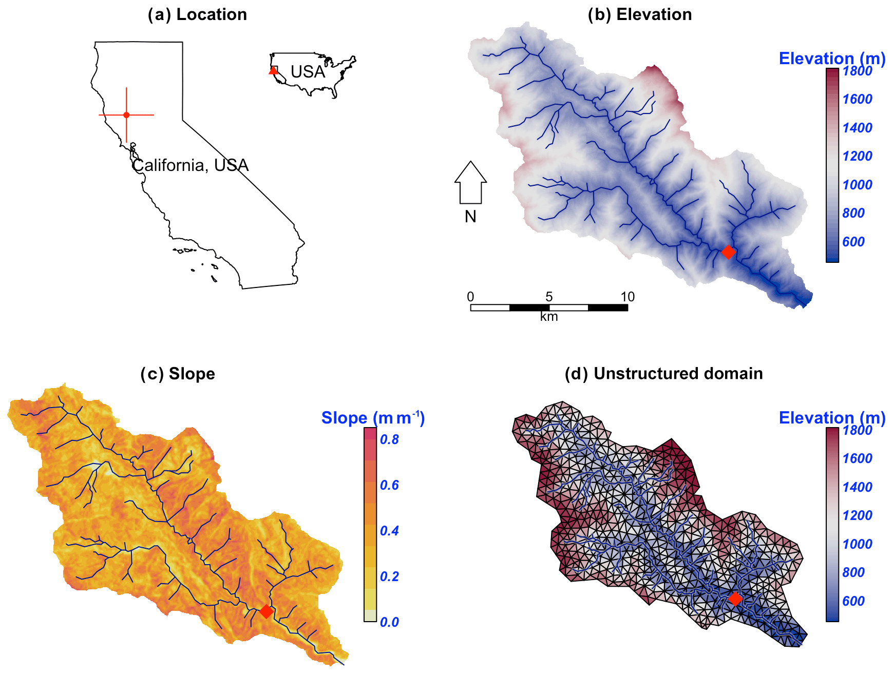
Figure 11 The location and terrestrial and hydrologic description of the Cache Creek in California. The red diamond in the map is the USGS gage station (11451100) used for calibration and validation.

Based on NLDAS-2 (Xia et al., 2012) from 2000 to 2017, the mean temperature and precipitation were 12.8 ^∘C and ∼817 mm, respectively, in this catchment. Precipitation varies seasonally; winter and spring are the primary wet seasons (Fig. 12).

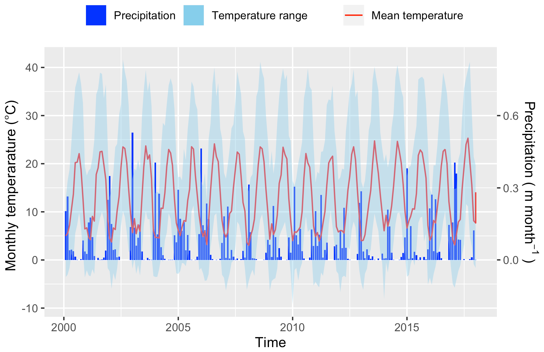
Figure 12 The monthly precipitation and temperature in Cache Creek based on NLDAS-2 data from 2000 to 2018. The blue ribbon is monthly precipitation in meters per month; the red line is monthly mean temperature, while the blue shaded region depicts the minimum and maximum temperature.

(McKay et al., 2012)(U.S. Geological Survey, 2016)(Soil Survey Staff, 2015)(Homer and Fry, 2012)(Xia et al., 2012)

Table 2 The basic data sources used to build the model domain of the Cache Creek Watershed.

Table 2 lists the geospatial and forcing data supporting hydrologic modeling in the CCW. The DEM is 30 m resolution raster data from National Elevation Dataset (NED) (U.S. Geological Survey, 2016). Forcing data, including precipitation, temperature, relative humidity, wind speed, and net radiation, are from NLDAS-2 (Xia et al., 2012, https://ldas.gsfc.nasa.gov/nldas/v2/forcing, last access: 19 December 2019). Our simulation in the CCW (Shu, 2019a) covers the period from 2000 to 2007. Because of the Mediterranean climate in this region, the simulation starts in summer to ensure adequate time before the October start to the water year. In our experiment, the first year (1 July 2000 to 30 June 2001) is the spin-up period, the following 2 years (1 July 2001 to 30 June 2003) are the calibration period, and the period from 1 July 2003 to 1 July 2007 is for validation.

The unstructured domain of the CCW (Fig. 11d) is built with rSHUD (Shu, 2020). The domain consists of 1147 triangular cells, with a mean area of 0.17 km². The total length of the river network is 126.5 km and consists of 103 river reaches in which the highest order of stream is 4. With a calibrated parameter set, the SHUD model (Shu, 2019a) took 5 h to simulate 18 years (2000–2017) in the CCW, with a nonparallel configuration (OpenMP is disabled on Mac Pro 2013 Xeon 2.7 GHz, 32 GB RAM).

Figure 13 reveals the comparison of simulated discharge against the observed discharge at the gage station of USGS 11451100 (https://waterdata.usgs.gov/ca/nwis/uv/?site_no=11451100, last access: 19 December 2019). The calibration procedure exploits the covariance matrix adaptation–evolution strategy (CMA-ES) to calibrate automatically (Hansen, 2016). The calibration program assigns 72 children in each generation and keeps the best child as the seed for the next generation, with limited perturbations. The perturbation for the next generation is generated from the covariance matrix of the previous generation. After 23 generations, the calibration tool identifies a locally optimal parameter set.

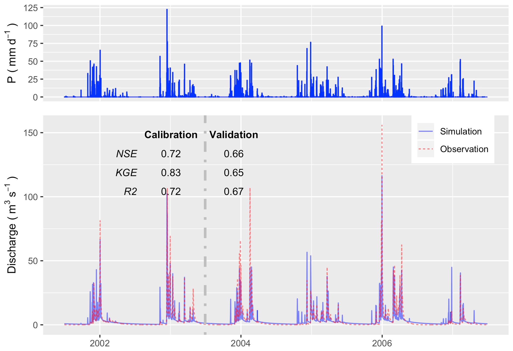
Figure 13 The hydrograph in Cache Creek (simulation versus observation) in the calibration (1 July 2001 to 30 June 2003) and validation periods (1 July 2003 to 30 June 2007).

Within the calibration period, Nash–Sutcliffe efficiency (NSE; Nash and Sutcliffe, 1970), Kling-Gupta efficiency (KGE; Gupta et al., 2009), and R² are 0.72, 0.83, and 0.72, respectively (Fig. 13). The goodness-of-fit in the validation period is less than calibration period (as expected), with NSE =0.66, KGE =0.67, and R²=0.65. Although the SHUD model captures the flood peaks after rainfall events, the magnitude of high flow in the hydrograph is less than the gage data. There are two potential causes of this bias: (1) underestimated precipitation intensity from NLDAS-2 data or (2) overfitting in the calibration, as the NSE tends to capture the mean value of the observational data rather than the extremes.

Figure 14 represents the monthly water balance in CCW, in which the PET is 3 times the annual precipitation, but the actual evapotranspiration (AET) is only 27 % of the precipitation. This result emerges because the summer is the peak of PET, while winter is the peak of precipitation and water availability. The AET is subjected to PET and water availability, so the maximum of AET occurs in early summer. The runoff ratio is about 73 %.

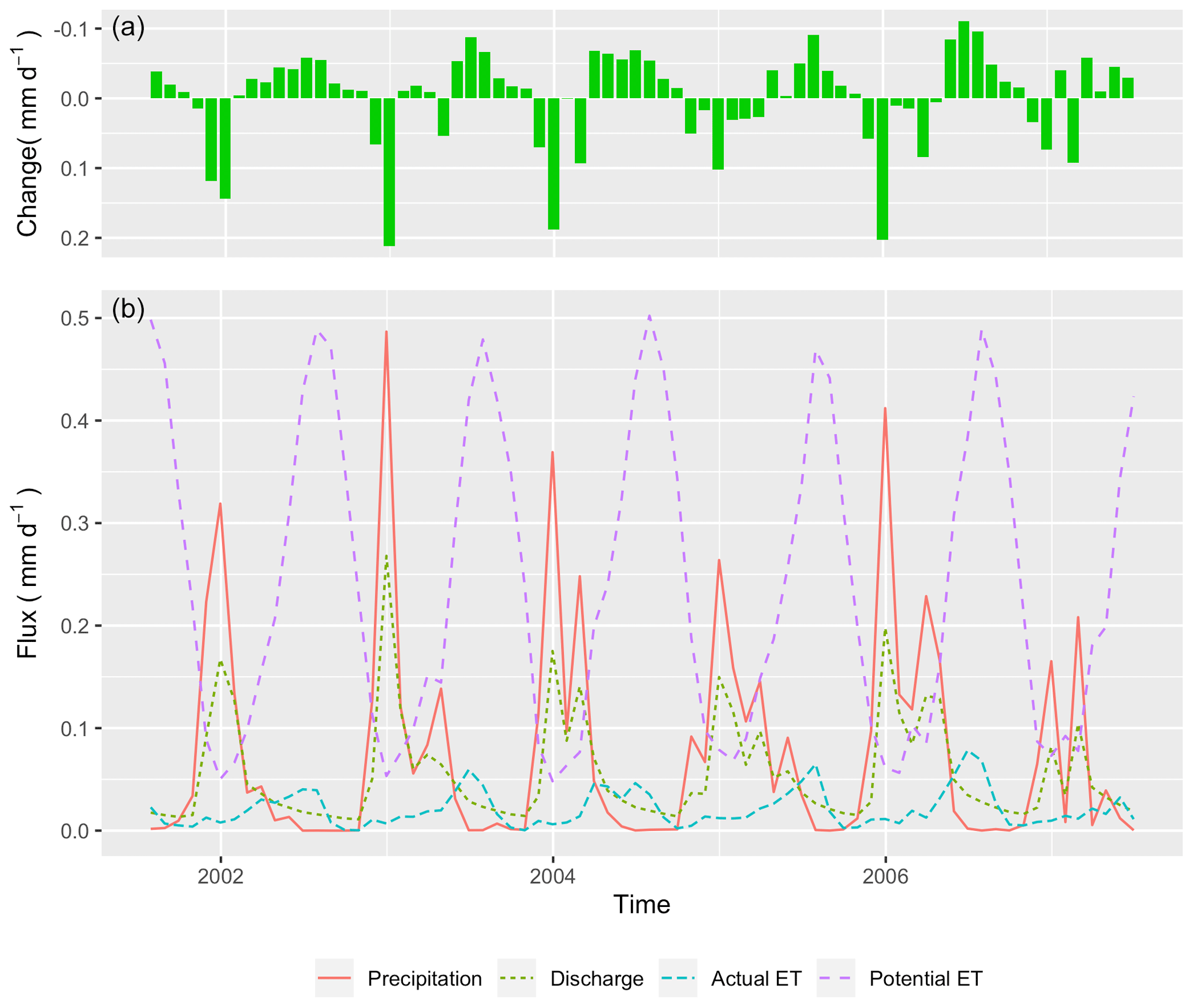
Figure 14 The monthly water balance trends in Cache Creek Watershed from 1 July 2001 to 30 June 2007. (a) Net change in water storage; (b) Fluxes of precipitation, actual evapotranspiration, potential evapotranspiration, and discharge at the outlet.

We use the groundwater distribution (Fig. 15) to demonstrate the spatial distribution of hydrologic metrics calculated from the SHUD model. Figure 15 illustrates the annual mean groundwater table in the validation period. Because the model fixes a 30 m aquifer, the results represent the groundwater within this 30 m aquifer only. The groundwater table and elevation along the green line on the map are extracted and plotted in Figure 15b. The gray ribbon is the 30 m aquifer, and the blue line is the location where groundwater storage is larger than zero. The light blue polygons (with the right axis for scale) are the groundwater storage along the cross section. The groundwater levels tend to follow the terrain, with groundwater accumulated in the valley or along relatively flat flood plains. In the CCW, groundwater does not stay on steep slopes suggesting the high conductivity of upland slopes.

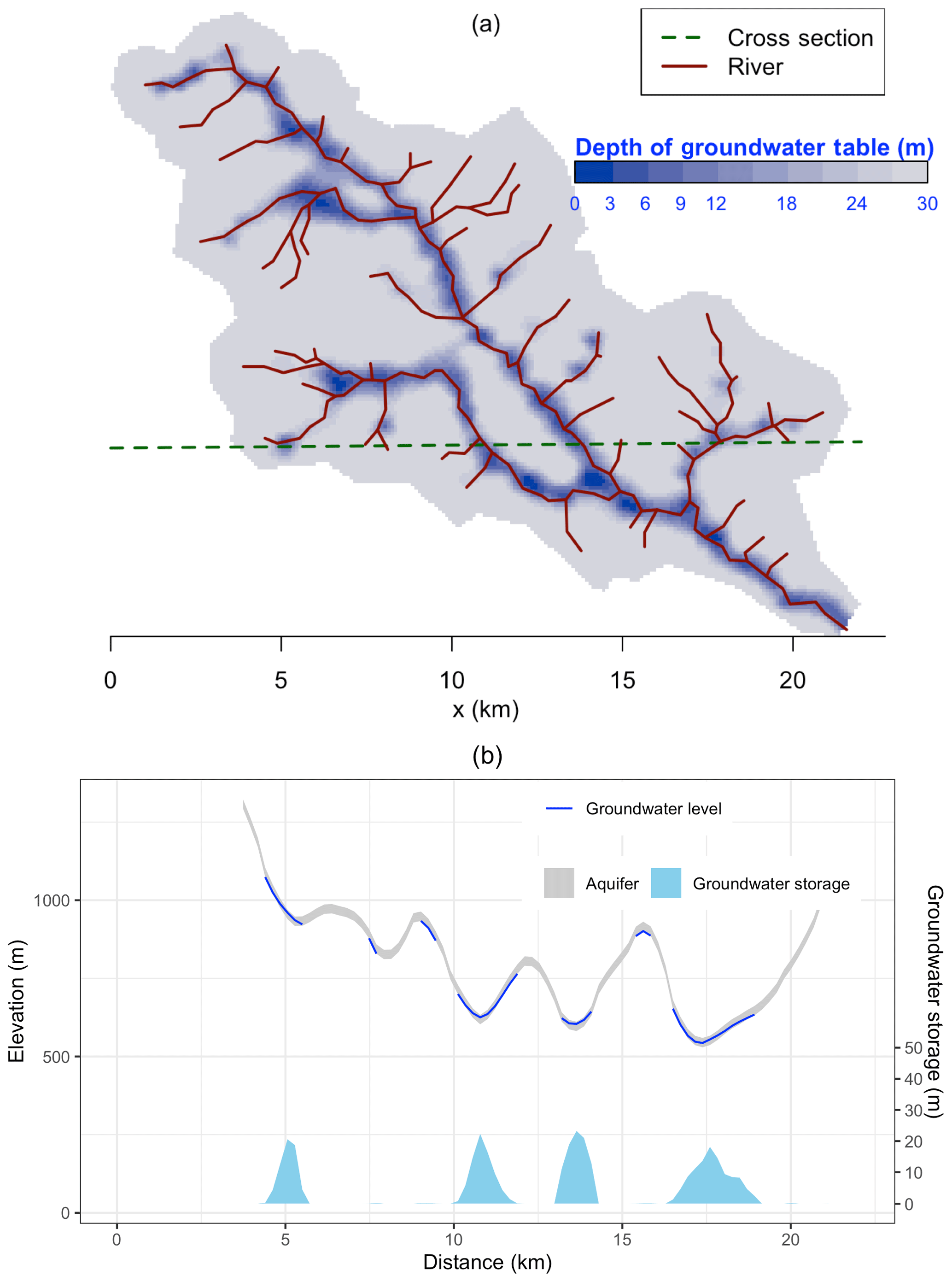
Figure 15 (a) Groundwater table and (b) the storage of groundwater in 30 m depth aquifer. The groundwater table and elevation along the green dashed line in (a) are extracted and plotted in (b). The gray ribbon is the 30 m aquifer, and the blue line is the groundwater table, only at the location where groundwater storage is larger than zero. The light blue polygons with the right axis are the groundwater storage along the cross section.

4 Summary of SHUD features and differences from PIHM

The features of the SHUD model are as follows:

• SHUD is a physically based process, spatially distributed catchment model. The model applies national geospatial data resources to simulate surface and subsurface flow in gaged or ungaged catchments. SHUD represents the spatial heterogeneity that influences the hydrology of the region based on national soil data and superficial geology. Several other groups have used PIHM, a SHUD ancestor to couple processes from biochemistry, reaction transport, landscape, geomorphology, limnology, and other related research areas.

• SHUD is a fully coupled hydrologic model, where the conservative hydrologic fluxes are calculated within the same time step. The state variables are the height of ponding water on the land surface, soil moisture, groundwater level, and river stage, while fluxes are infiltration, overland flow, groundwater recharge, lateral groundwater flow, river discharge, and exchange between river and hillslope cells.

• The global ODE system in SHUD is solved with a state-of-the-art parallel ODE solver, known as CVODE (Hindmarsh et al., 2005) developed at Lawrence Livermore National Laboratory.

• SHUD permits adaptable temporal and spatial resolution. The spatial resolution of the model varies from centimeters to kilometers based on modeling requirements computing resources. The internal time step of the iteration is adjustable and adaptive; it can export the status of a catchment at time intervals from minutes to days. The flexible spatial and temporal resolution of the model makes it valuable for coupling with other systems.

• SHUD can estimate either a long-term hydrologic yield or a single-event flood.

• SHUD is an open-source model, available on GitHub (Shu, 2019b).

4.1 Differences from PIHM

As a descendant of PIHM, SHUD inherits many fundamental ideas and the conceptual structure from PIHM, including the solution of hydrologic variables using CVODE. The code has been completely rewritten in a new programming language, with a new discretization and corresponding improvements to the underlying algorithms, adapting new mathematical schemes and flexible input/output data formats. Although SHUD is forked from PIHM, SHUD still inherits the use of CVODE for solving the ODE system but modernizes and extends PIHM's technical and scientific capabilities. The major differences are as follows:

1. SHUD is written in C++, an object-oriented programming language with functionality to avoid memory leaks from C. Most of the functions in SHUD do not exist in PIHM, which are newly defined because of the brand-new design of the SHUD model. Only a few functions related to physical equations, such as Manning's equation and van Genuchten's equation, are shared in SHUD and PIHM. So although SHUD and PIHM follow a similar fundamental perceptual model, they follow different mathematical and computational strategies.

2. SHUD implements a redesign of the calculation of water exchange between hillslope and river. The PIHM defines the river channel as adjacent to bank cells – namely, the river channel shares the edges with bank cells. This design leads to sink problems in cells that share one node with a starting river channel that can reduce simulation performance.

3. Although the mathematical equations underlying SHUD are generally the same as PIHM, the numerical formulation of processes, the coupling strategy, and input/output structures have been greatly enhanced. Common computations in different functions within various processes are extracted and defined as shared inline functions, maintaining calculation consistency and facilitating code updates. The elimination of redundant variables and functions also advances consistency and efficiency.

4. SHUD adds mass-balance control within the calculation of each layer of cells and river channels, important for accurate and efficient long-term and microscale hydrologic modeling.

5. The internal data structure and external input/output formats have been redesigned for efficiency and user-friendly formats supporting ASCII and binary. The binary format is particularly important for efficient writing and postprocessing over numerous model domains.

We now briefly summarize the technical model improvements and technical capabilities of the model compared to PIHM. This elaboration of the relevant technical features aims to assist future developers and advanced users with model coupling. Compared with PIHM, SHUD (Shu, 2019b) does the following:

• supports compatibility with the implicit Sundial/CVODE solver version 5.0 (the most recent version at the time of writing) and above;

• supports OpenMP parallel computation;

• utilizes object-oriented programming (C++);

• supports human-readable input/output files and filenames;

• exposes unified functions to handle the time-series data (TSD) (in a standardized spreadsheet format), including forcing, leaf area index, roughness length, boundary conditions, and melting factor;

• exports model initial condition at specific intervals that facilitate warm starts of continuous simulation;

• automatically checks the range of physical parameters and forcing data;

• adds a debug mode that monitors potential errors in parameters and memory operations; and

• includes a series of R codes for pre- and postprocessing data, visualization, and data analysis (that will be discussed in future work).

5 Conclusions

The Simulator for Hydrologic Unstructured Domains (SHUD) is a multiprocess, multiscale, and multitemporal model that integrates major hydrologic processes and solves the physical equations with the finite volume method. The governing equations are solved within an unstructured mesh domain consisting of triangular cells. The variables used for the surface, vadose layer, groundwater, and river routing are fully coupled together with a fine time step. The SHUD uses the 1-D unsaturated flow and 2-D groundwater flow. River channels connect with hillslope via overland flow and baseflow. The model, while using distributed terrestrial characteristics (from climate, land use, soil, and geology) and preserving their heterogeneity, supports efficient performance through parallel computation.

SHUD is a robust integrated modeling system that has the potential for providing scientists with new insights into their domains of interest and will benefit the development of coupling approaches and architectures that can incorporate scientific principles. The SHUD modeling system can be used for applications in (1) hydrologic studies from hillslope scale to regional scale; area of the model domain ranges from 1 m² to 10⁶ km²; (2) water resource and stormwater management; (3) coupling research with related fields, such as limnology, agriculture, geochemistry, geomorphology, water quality, and ecology; (4) climate change; and (5) land-use change. In summary, SHUD is a valuable scientific tool for any modeling task associating with hydrologic responses.

Appendix A: Nomenclature

Evapotranspiration Calculation
Δ	Slope vapor pressure curve (kPa ∘C−1)
γ	Psychrometric constant (kPa ∘C−1)
λ	Latent heat of vaporization (MJ kg−1)
ρa	Density of Air (kg m−3)
cp	Specific heat at constant pressure (MJ kg−1 ∘C−1)
ea	Actual vapor pressure (kPa)
es	Saturation vapor pressure (kPa)
G	Soil heat flux density (MJ m−2 s−1)
Rn	Net radiation at the crop surface (MJ m−2 s−1)
rs	Surface resistance of vegetation (s m−1)
ra	Aerodynamic resistance (s m−1)
Hydrologic metrics
α	van Genuchten soil parameter (m−1)
αh	Horizontal macropore areal fraction (m2 m−2)
αimp	Impervious area fraction (m2 m−2)
αv	Vertical macropore areal fraction (m2 m−2)
αveg	Vegetation fraction (m2 m−2)
$\overline{K}$	Average conductivity (m s−1)
$\overline{y}$	Effective height of overland flow between two adjacent cells (m)
β	van Genuchten soil parameter (–)
βs	Soil moisture stress to evapotranspiration (–)
Δt	Time interval between consequential time steps (m)
$\stackrel{\mathrm{‾}}{y_{\mathrm{gw}}}$	Effective water height for groundwater flow calculation (m)
$\stackrel{\mathrm{‾}}{y_{\mathrm{sf}}}$	Effective water height for overland flow calculation (m)
ψ	Soil matrix potential head (m)
θ	Soil moisture content (m3 m−3)
Θ	Relative saturation ratio (–)
θfc	The soil moisture content of field capacity (m3 m−3)
θr	Residual soil moisture content (m3 m−3)
θs	Porosity of soil (m3 m−3)
Ar	Area of river open water (m2)
Ac	Area of a cell (m2)
bg	Effective height of groundwater flow between the river segment and hillslope cell (m)
bs	Effective height of overland flow between the river segment and hillslope cell (m)
Cw	Coefficient of discharge (m)
Cic	Coefficient of interception (m)
Dus	The deficit of soil column; thickness of vadose layer (m)

dj	Distance between centroids of the current cell and neighbor j (m)
drb	Thickness of river bed; for calculation of baseflow to rivers (m)
E0	Potential evapotranspiration (m s−1)
Ec	Evaporation from interception (m s−1)
Es	Evaporation from soil (m s−1)
Esm	Evaporation from the soil matrix (m s−1)
Esp	Evaporation from ponding water on land surface (m s−1)
Et	Transpiration (m s−1)
Etg	Transpiration from saturated layer (m s−1)
Etg	Transpiration from saturated layer (m s−1)
Hcgw	Hydraulic head of water in cell groundwater (m)
Hcsf	Hydraulic head of water on land surface (m)
Hriv	Hydraulic head in a river channel (m)
Kei(Θ)	Effective infiltration conductivity (m s−1)
Ker	Effective recharge conductivity (m s−1)
Keg	Effective horizontal conductivity (m s−1)
kg	Saturated horizontal conductivity (m s−1)
kv	Saturated vertical conductivity of saturated layer (m s−1)
km	Saturated conductivity of soil macropore (m s−1)
Kr(Θ)	Relative conductivity, which is a function of saturation ratio (–)
krb	Saturated conductivity of the river bed (–)
kx	Saturated conductivity of the top soil (m s−1)
Lj	Length of edge j of a cell (m)
Ls	Length of river segment that overlay with a cell (m)
LAI	Leaf area index (m2 m−2)
mf	Snow melting factor (m s−1 ∘C−1)
n	Manning's roughness (s m${}^{-\mathrm{1}/\mathrm{3}}$)
Nc	Number of cells overlaying a river reach (–)
Nu	Number of upstream reaches flowing to a river reach (–)
P	Atmospheric precipitation or irrigation (m s−1)
Pn	Net precipitation (m s−1)
Psn	Snowfall (m s−1)
Qdn	Volume flux to the downstream river channel (m3 s−1)
Qg	Groundwater flow between two cells (m3 s−1)
Qgr	Volume flux between river and cells via groundwater flow (m3 s−1)
qi	Infiltration rate, positive is downward (m s−1)
qr	Recharge rate, positive is downward (m s−1)

Qs	The overland flow between two cells (m3 s−1)
qsn	Snow melting rate (m s−1)
Qsr	Volume flux between river and hillslope cells via overland flow (m3 s−1)
Qup	Volume flux from upstream river reaches (m3 s−1)
s0	The slope of land surface (m m−1)
Sic	Water storage of interception layer (canopy) (m)
$S_{\mathrm{ic}}^{*}$	Maximum interception capacity (m)
Ssn	Snow storage (m)
sy	Specific yield (m m−1)
T	Air temperature (∘C)
ygw	Groundwater head (above impervious bedrock) of a cell (m)
yriv	River stage in a river channel (m)
ysf	Surface water storage in a cell (m)
yus	Unsaturated storage equivalence of a cell (m)
zb	Elevation of impervious bedrock from the datum (m)
zbank	Elevation of the riverbank from the datum (m)
zgw	Elevation of groundwater table from the datum (m)
zm	Elevation of macropore from the datum (m)
zsf	Elevation of land surface from the datum (m)
T0	Temperature threshold for snow melt to occur (∘C)
Variables used in CVODE
Y0	The initial conditions to start the simulation (m)
Ygw	Vector of cell groundwater head (above impervious bedrock) (m)
Yriv	Vector of river stage in all river channels (m)
Ysf	Vector of surface water storage of all cells (m)
Yus	Vector of unsaturated storage equivalence of all cells (m)
Y	Vector of conserved state variables in CVODE (m)
t	Time (s)
tn−1	Previous time (s)
tn	Current time (s)