HydroMix v1.0: a new Bayesian mixing framework for attributing uncertain hydrological sources

Tracers have been used for over half a century in hydrology to quantify water sources with the help of mixing models. In this paper, we build on classic Bayesian methods to quantify uncertainty in mixing ratios. Such methods infer the probability density function (PDF) of the mixing ratios by formulating PDFs for the source and target concentrations and inferring the underlying mixing ratios via Monte Carlo sampling. However, collected hydrological samples are rarely abundant enough to robustly fit a PDF to the source concentrations. Our approach, called HydroMix, solves the linear mixing problem in a Bayesian inference framework wherein the likelihood is formulated for the error between observed and modeled target variables, which corresponds to the parameter inference setup commonly used in hydrological models. To address small sample sizes, every combination of source samples is mixed with every target tracer concentration. Using a series of synthetic case studies, we evaluate the performance of HydroMix using a Markov chain Monte Carlo sampler. We then use HydroMix to show that snowmelt accounts for around 61 % of groundwater recharge in a Swiss Alpine catchment (Vallon de Nant), despite snowfall only accounting for 40 %–45 % of the annual precipitation. Using this example, we then demonstrate the flexibility of this approach to account for uncertainties in source characterization due to different hydrological processes. We also address an important bias in mixing models that arises when there is a large divergence between the number of collected source samples and their flux magnitudes. HydroMix can account for this bias by using composite likelihood functions that effectively weight the relative magnitude of source fluxes. The primary application target of this framework is hydrology, but it is by no means limited to this field.

1 Introduction

Most water resources are a mixture of different water sources that have traveled via distinct flow paths in the landscape (e.g., streams, lakes, groundwater). A key challenge in hydrology is to infer source contributions to understand the flow paths to a given water body using a source attribution technique. A classic example is the two-component hydrograph separation model to quantify the proportion of groundwater and rainfall in streamflow, often referred to as “pre-event” water vs. “event” water (Burns et al., 2001; Klaus and McDonnell, 2013; Schmieder et al., 2016). Other examples include estimating the proportional contribution of rainfall and snowmelt to groundwater recharge (Beria et al., 2018; Jasechko et al., 2017; Jeelani et al., 2010), fog to the amount of throughfall (Scholl et al., 2011, 2002; Uehara and Kume, 2012), and soil moisture (at varying depths) and groundwater to vegetation water use (Ehleringer and Dawson, 1992; Evaristo et al., 2017; Rothfuss and Javaux, 2017).

The primary goal of such attribution in hydrology is to infer the contribution of different sources to a target water body; the tracer can be an observable compound like a dye, a conservative solute, or even a proxy for chemical composition such as electrical conductivity. The key requirement is that the concentration of the tracer is distinguishable between different sources. The stable isotope compositions of hydrogen and oxygen in water (subsequently referred to as “stable isotopes of water”) are used as tracers in hydrology. Other commonly used tracers include electrical conductivity (Hoeg et al., 2000; Laudon and Slaymaker, 1997; Lopes et al., 2018; Pellerin et al., 2007; Weijs et al., 2013) and conservative geochemical solutes such as chloride and silica (Rice and Hornberger, 1998; Wels et al., 1991).

Classically, attribution analysis is done by assigning an average tracer concentration to each source, typically estimated from time or space averages of observed field data (Maule et al., 1994; Winograd et al., 1998), and then solving a series of linear equations. In order to express uncertainty in the attribution analysis, a tracer-based hydrograph separation approach was first proposed in the work of Genereux (1998) and has subsequently been used in many studies (Genereux et al., 2002; Koutsouris and Lyon, 2018; Zhu et al., 2019). Bayesian mixing approaches offer a useful alternative to classic hydrograph separation, as Bayesian approaches explicitly acknowledge the temporal variability of source tracer concentrations estimated from observed samples (Barbeta and Peñuelas, 2017; Blake et al., 2018). Rather than a single estimate of source contributions, Bayesian approaches yield full probability density functions (PDFs) of the fraction of different sources in the target mixture (Parnell et al., 2010; Stock et al., 2018), hereafter referred to as “mixing ratios”.

Bayesian mixing was first developed in ecology to estimate the proportion of different food sources to animal diets (Parnell et al., 2010; Stock et al., 2018). Hydrological applications of such models are still rare (Blake et al., 2018; Evaristo et al., 2016, 2017; Oerter et al., 2019). In a Bayesian mixing model, a statistical distribution is fitted to both the measured source tracer concentrations and to the measured tracer concentrations from the target (e.g., river, groundwater, vegetation). The distribution of the mixing ratios is then inferred via Bayesian inference. With recent advances in probabilistic programming languages like Stan (Carpenter et al., 2017), Bayesian inference has become a relatively simple task.

However, the key limitation with the above approach is that the source compositions are assumed to come from standard statistical distributions. Typically, the sources are assumed to be drawn from Gaussian distributions, which can be fully characterized by the mean and variance of the data available for each source (Stock et al., 2018). This limits both the potential applicability and the insights that can be gained from tracer information in hydrology because the sample mean and variance may not accurately reflect the statistical properties of the actual source composition, and the Gaussian approach represents an unnecessary simplification in cases in which a large amount of information on source composition is available.

An additional complication in hydrology comes from the fact that observed point-scale samples do not necessarily capture the tracer concentrations in the actual sources, which are distributed heterogeneously in space and whose contribution can be temporally variable depending on the state of the catchment (Harman, 2015). For instance, if we were to characterize the contribution of snowmelt to groundwater, we would need to capture (1) the temporal evolution of the isotopic ratio of snowmelt, which strongly varies in space (Beria et al., 2018; Earman et al., 2006), and (2) the temporal evolution of the area actually covered by snow. This spatially and temporally distributed nature of the sources can be hard to account for in both analytical and Bayesian mixing approaches.

To overcome the limitations of source heterogeneity and the previously discussed restriction to Gaussian distributions, we present a new mixing approach for hydrological applications called HydroMix. This approach does not require a parametric description of observed source or target tracer concentrations. Instead, HydroMix formulates the linear mixing problem in a Bayesian inference framework similar to hydrological rainfall–runoff models (Kavetski et al., 2006a), wherein the mixing ratios of the different sources are treated as model parameters. Multiple model parameters can be inferred in such a setup, allowing for the parameterization of additional hydrologic processes that can modify source tracer concentrations (shown in Sect. 3.5). A more detailed account of the advantages and limitations of this new approach is given in Sect. 5.

In this paper, we first describe the theoretical details of HydroMix for a simple case study with two sources, one mixture and one tracer (Sect. 2). Section 3 presents synthetic and real-world case studies that demonstrate the accuracy, robustness, and flexibility of HydroMix. In the synthetic case study, we use a conceptual hydrologic model to simulate tracer concentrations. We also introduce a composite likelihood function that accounts for the magnitude of the different source fluxes. The real-world case study applies HydroMix in a high-elevation headwater catchment in Switzerland. The results of these applications are presented in Sect. 4 before summarizing the main outcomes, applicability, and limitations of HydroMix in Sect. 5.

2 Model description and implementation

A system with n sources mixing linearly in a target water body can be written as

$$\begin{array}{}\text{(1)}& {\mathit{\rho }}_{\mathrm{1}}{S}_{\mathrm{1}}^k+{\mathit{\rho }}_{\mathrm{2}}{S}_{\mathrm{2}}^k+\mathrm{\dots }+{\mathit{\rho }}_n{S}_n^k=Y^k,\end{array}$$

where Y^k is the concentration of the kth tracer in the target mixture, and $S_i^k$ is the concentration of the kth tracer in source i; ρ_i(i=1,...,n) represents the fractions of all sources in the mixture, with ${\sum }_{i=\mathrm{1}}^n{\mathit{\rho }}_i=\mathrm{1}$, corresponding to the aggregation of different sources in the mixture. In order to solve this system of linear equations, n−1 different tracers are required.

Section 2.1 details the general modeling approach for a simplified system with two sources and one tracer. This is followed by a detailed discussion on the choice of the parameter inference approach used.

Linear mixing model with non-concomitant observed data

For a system with two sources that combine linearly to form a mixture, the mixing model can be formulated as

$$\begin{array}{}\text{(2)}& \mathit{\rho }{S}_{\mathrm{1}}\left(t-{\mathit{\tau }}_{\mathrm{1}}\right)+\left(\mathrm{1}-\mathit{\rho }\right)S_{\mathrm{2}}\left(t-{\mathit{\tau }}_{\mathrm{2}}\right)=Y\left(t\right),\end{array}$$

where S₁(t−τ₁) is the tracer concentration in source 1 at time step t−τ₁, S₂(t−τ₂) is the tracer concentration in source 2 at time step t−τ₂, Y(t) is the concentration of the mixture (i.e., the tracer concentration in the target) at time step t, ρ is the mixing ratio, and τ_i is the time delay between the time when source i enters the system and the time when it is observed in the mixture. As an example, for a case in which the two sources are snowmelt and rainfall and the mixture is groundwater, ρ represents the proportional groundwater recharged from snowmelt and τ represents the average time lag for rain or snowmelt to reach groundwater once they enter the soil. In other words, the time lag (τ) stands for any delay caused by tracer transport from the source to the output; we assume that the source components are conservative in nature.

The two parameters in this system, the mixing ratio (ρ) and the time delay (τ), can be inferred via classical Bayesian parameter inference, which is widely used in hydrology (Kavetski et al., 2006a, b; Schaefli and Kavetski, 2017). This implies taking an observed time series of the target (e.g., the tracer concentration in groundwater) and building a vector of model residuals:

$$\begin{array}{}\text{(3)}& {\mathit{\epsilon }}_t={\stackrel{\mathrm{̃}}{Y}}_t-{\widehat{Y}}_t,\end{array}$$

where ${\stackrel{\mathrm{̃}}{Y}}_t$ represents the observed mixture concentration and ${\widehat{Y}}_t$ represents the simulated mixture concentration. However, in real environmental systems like that of groundwater recharge from rainfall and snowmelt, there are four major difficulties that can prevent the inference of ρ and τ from the observed data.

• i.

  ρ and τ strongly vary in time depending on catchment conditions such as soil moisture (as previously discussed in the context of the “inverse storage effect”; Benettin et al., 2017; Harman, 2015).

• ii.

  Long time series of the tracer concentration in both the sources and mixture are rare.

• iii.

  The effect of seasonality in precipitation can make the inference of τ very difficult in the case that the goal is to understand intra-annual recharge dynamics.

• iv.

  The tracer concentrations in the different sources are generally measured at point scales, whereas the tracer concentration in the target integrates inputs over the entire source area.

Our practical solution to limitation (iv) is to assume that tracer concentrations in the two sources are functions of observable point processes:

$$\begin{array}{}\text{(4)}& S_i\left(t\right)=f_i\left(P_i\left(t\right)\right),\end{array}$$

where the function f_i represents the transformation from the point to the catchment scale for source i. Limitation (iii) can be relaxed by assuming a long enough time step (e.g., long-term groundwater recharge dynamics), for which the observed samples are samples from the long-term (>>1 year) source and target compositions. This allows us to replace the time step t and t+τ with Δt and write Eq. (2) as

$$\begin{array}{}\text{(5)}& \mathit{\rho }{S}_{\mathrm{1}}^{\prime }\left(\mathrm{\Delta }t\right)+\left(\mathrm{1}-\mathit{\rho }\right)S_{\mathrm{2}}^{\prime }\left(\mathrm{\Delta }t\right)=Y^{\prime }\left(\mathrm{\Delta }t\right),\end{array}$$

where the ^′ signifies the new time-integrated variables. Now, any observed point-scale tracer concentration p_i in a given source i or in the output (e.g., the isotopic ratio of snowmelt) can be assumed to represent a sample from a stationary process (from $S_{\mathrm{1}}^{\prime }$, $S_{\mathrm{2}}^{\prime }$, or Y^′). This assumption is in fact implicitly underlying most of the existing hydrological mixing models in which point samples are used to characterize a spatial process and the time reference of the samples is discarded.

By utilizing all the available measurements $\mathit{\{}{p}_{\mathrm{1}}{}^{\prime }{\mathit{\}}}_{i=\mathrm{1}\mathrm{\dots }n}$ and $\mathit{\{}{p}_{\mathrm{2}}{}^{\prime }{\mathit{\}}}_{j=\mathrm{1}\mathrm{\dots }m}$ of the two sources in the above model, with n samples of source 1 and m samples of source 2, we can build n×m predictions and compare them with the q observed samples of the target as

$$\begin{array}{}\text{(6)}& {\mathit{\epsilon }}_{ij}^k={\stackrel{\mathrm{̃}}{Y}}_{\mathrm{obs}}^k-{\widehat{Y}}_{ij},\end{array}$$

where ${\stackrel{\mathrm{̃}}{Y}}_{\mathrm{obs}}^k$ is the kth observed target concentration out of a total number of q target concentrations.

Assuming that the residuals can be described with a Gaussian error model with a mean of zero and constant variance σ²,

$$\begin{array}{}\text{(7)}& \mathit{\epsilon }\sim N\left(\mathrm{0},{\mathit{\sigma }}^{\mathrm{2}}\right),\end{array}$$

we can compute the likelihood function of the residuals as the joint probability of all the residuals:

$$\begin{array}{}\text{(8)}& \begin{array}{rl}{L}_j& ({\stackrel{\mathrm{̃}}{Y}}_{\mathrm{obs}}\mathrm{|}{P}_{\mathrm{1}},P_{\mathrm{2}},\mathit{\theta })={\prod }_{k=\mathrm{1}}^q{\prod }_{j=\mathrm{1}}^m{\prod }_{i=\mathrm{1}}^n(\mathrm{2}\mathit{\pi }{\mathit{\sigma }}^{\mathrm{2}}{)}^{-\mathrm{0.5}}\\ & \exp \left(-{\displaystyle \frac{\mathrm{1}}{\mathrm{2}}}{\displaystyle \frac{{\left({\stackrel{\mathrm{̃}}{Y}}_{\mathrm{obs}}^k-{\widehat{Y}}_{ij}\right)}^{\mathrm{2}}}{{\mathit{\sigma }}^{\mathrm{2}}}}\right),\end{array}\end{array}$$

where θ represents all the model parameters and P_i(i=1, 2) is the observed point process (see Eq. 4). The above Gaussian error model could in principle be replaced with any other stochastic process. However, the Gaussian error model has been shown to be relatively robust in this kind of application (Lyon, 2013; Schaefli and Kavetski, 2017).

In the case of linear mixing between two sources, the two model parameters considered at this stage are the mixing ratio ρ and the error variance σ². The error variance can either be computed from the observed residuals or treated as a model parameter (Kuczera and Parent, 1998; Schaefli et al., 2007). For the examples shown in this paper, the error variance is computed from the residuals.

In order to avoid numerical problems, we use the log-likelihood form of Eq. (8),

$$\begin{array}{}\text{(9)}& \begin{array}{rl}\log L_j& ({\stackrel{\mathrm{̃}}{Y}}_{\mathrm{obs}}\mathrm{|}{P}_{\mathrm{1}},P_{\mathrm{2}},\mathit{\theta })={\sum }_{k=\mathrm{1}}^q{\sum }_{j=\mathrm{1}}^m{\sum }_{i=\mathrm{1}}^n\\ & -\mathrm{0.5}\left[\log \left(\mathrm{2}\mathit{\pi }{\mathit{\sigma }}^{\mathrm{2}}\right)+{\displaystyle \frac{{\left({\stackrel{\mathrm{̃}}{Y}}_{\mathrm{obs}}^k-{\widehat{Y}}_{ij}\right)}^{\mathrm{2}}}{{\mathit{\sigma }}^{\mathrm{2}}}}\right],\end{array}\end{array}$$

for parameter inference in a Bayesian framework.

Following the general Bayes' equation, the posterior distribution of the model parameters can be written as

$$\begin{array}{}\text{(10)}& p\left(\mathit{\theta }|P_{\mathrm{1}},P_{\mathrm{2}},\stackrel{\mathrm{̃}}{Y}\right)={\displaystyle \frac{p\left(\stackrel{\mathrm{̃}}{Y}\mathrm{|}\mathit{\theta },P_{\mathrm{1}},P_{\mathrm{2}}\right)p\left(\mathit{\theta }\right)}{p\left(\stackrel{\mathrm{̃}}{Y}|P_{\mathrm{1}},P_{\mathrm{2}}\right)}},\end{array}$$

where p(θ) is the prior distribution of the model parameters and $p\left(\stackrel{\mathrm{̃}}{Y}\mathrm{|}\mathit{\theta },P_{\mathrm{1}},P_{\mathrm{2}}\right)$ is the likelihood function. The denominator of Eq. (10) can generally not be computed as that would require integration over the whole parameter space, which is computationally expensive, and that is why Eq. (10) is reduced to

$$\begin{array}{}\text{(11)}& p\left(\mathit{\theta }|P_{\mathrm{1}},P_{\mathrm{2}},\stackrel{\mathrm{̃}}{Y}\right)\propto p\left(\stackrel{\mathrm{̃}}{Y}\mathrm{|}\mathit{\theta },P_{\mathrm{1}},P_{\mathrm{2}}\right)p\left(\mathit{\theta }\right).\end{array}$$

Two methods are traditionally used in hydrology to sample from the posterior distribution from Eq. (11): Markov chain Monte Carlo (MCMC) sampling (Hastings, 1970; Metropolis and Ulam, 1949) and importance sampling (Glynn and Iglehart, 1989; Neal, 2001). In the case of MCMC sampling, a common approach is the Metropolis algorithm (Kuczera and Parent, 1998; Schaefli et al., 2007; Vrugt et al., 2003). In importance sampling, the posterior distribution is obtained from weighted samples drawn from the so-called importance distribution. For typical multivariate hydrological problems, the only possible choices for the importance distribution are either uniform sampling over a hypercube or sampling from an over-dispersed multi-normal distribution (Kuczera and Parent, 1998). A stochastic process is defined as over-dispersed when the variance of the underlying distribution is greater than its mean (Inouye et al., 2017). The sampling distributions in such cases have large variance, allowing for sufficient sampling over the entire parameter range.

We implement an MCMC sampling algorithm using a Metropolis–Hastings (Hastings, 1970) criterion to infer the posterior distribution of the mixing ratio. For the synthetic case study (Sect. 3.1), we set up 10 parallel MCMC chains to monitor convergence according to the classical Gelman–Rubin convergence criterion (Gelman and Rubin, 1992). Each chain is initiated by assigning a uniform prior distribution for the mixing ratio, and the mixing ratio varies between 0 and 1. For the subsequent case studies, we use importance sampling for the sake of simplicity. The prior distributions of additional model parameters (if applicable) are discussed in the corresponding case study section. Apart from the prior distribution of the model parameters, HydroMix requires tracer concentration of the different sources and of the mixture. The error model variance is not jointly inferred with other model parameters but calculated for each sample parameter set from the residuals according to Eq. (6).

3 Case studies

We provide a comprehensive overview of the performance of HydroMix based on a set of synthetic case studies (case studies in Sect. 3.1 and 3.2) and a real-world application to demonstrate the practical relevance for hydrologic applications (case studies in Sect. 3.4 and 3.5). The first case study demonstrates the ability of HydroMix to converge on the correct posterior distribution for synthetically generated data. The second case study uses a synthetic dataset of rain, snow, and groundwater isotopic ratios using a conceptual hydrologic model and compares the results of HydroMix to the actual mixing ratios assumed to generate the dataset. It then weights the source samples and evaluates the effect of weighting on the mixing ratio (case study in Sect. 3.3). In the last two case studies, HydroMix is applied to observed tracer data from an Alpine catchment in the Swiss Alps to infer source mixing ratios and an additional parameter (isotopic lapse rate).

3.1 Mixing using Gaussian distributions

In this example, source concentrations S₁ and S₂ are drawn from two Gaussian distributions with different means (μ₁,μ₂) and standard deviations (σ₁,σ₂) and combined to form the mixture Y with a constant mixing ratio ρ:

$$\begin{array}{}\text{(12)}& \mathit{\rho }{S}_{\mathrm{1}}+(\mathrm{1}-\mathit{\rho })S_{\mathrm{2}}=Y.\end{array}$$

Assuming the two distributions are independent, the resultant mixture is normally distributed with mean (μ_y) and variance $\left({\mathit{\sigma }}_y^{\mathrm{2}}\right)$ defined as

$$\begin{array}{}\text{(13)}& {\mathit{\mu }}_y=\mathit{\rho }{\mathit{\mu }}_{\mathrm{1}}+\left(\mathrm{1}-\mathit{\rho }\right){\mathit{\mu }}_{\mathrm{2}};{\mathit{\sigma }}_y^{\mathrm{2}}={\mathit{\rho }}^{\mathrm{2}}{\mathit{\sigma }}_{\mathrm{1}}^{\mathrm{2}}+(\mathrm{1}-\mathit{\rho }{)}^{\mathrm{2}}{\mathit{\sigma }}_{\mathrm{2}}^{\mathrm{2}}.\end{array}$$

A given number of samples are drawn from the distributions of S₁ and S₂ and of the mixture Y. The posterior distribution of the mixing ratio, $p\left(\mathit{\rho }|\stackrel{\mathrm{̃}}{S_{\mathrm{1}}},\stackrel{\mathrm{̃}}{S_{\mathrm{2}}},\stackrel{\mathrm{̃}}{Y}\right)$, is then inferred using HydroMix for (i) a case in which the two source distributions are clearly identifiable and (ii) a case in which the distributions have a large overlap. Different values of mixing ratios are tested, with ratios varying from 0.05 to 0.95 in steps of 0.05.

The sensitivity of HydroMix to the number of samples drawn from S₁, S₂, and Y, along with the time to convergence, is assessed based on the sum of the absolute error between the estimated mixing ratio $\widehat{\mathit{\rho }}$ and its true value ρ.

3.2 Mixing with a time series generated using a hydrologic model

In this case study, we build a conceptual hydrologic model wherein groundwater is assumed to be recharged directly from rainfall and snowmelt. Stable isotopes of deuterium (δ²H) are used to see how the isotopic ratio in groundwater evolves under different assumptions of rain and snow recharge efficiencies.

Synthetic time series are generated for precipitation, the isotopic ratio in precipitation, and air temperature at a daily time step. For generating the precipitation time series, the time between two successive precipitation events is assumed to be a Poisson process with the precipitation intensity following an exponential distribution (Botter et al., 2007; Rodriguez-Iturbe et al., 1999). Time series of air temperature and of isotopic ratios in precipitation are obtained by generating an uncorrelated Gaussian process with the mean following a sine function (to emulate a seasonal signal) and with constant variance (Allen et al., 2018; Parton and Logan, 1981). The separation of precipitation into rainfall (P_r) and snowfall (P_s) is done based on a temperature threshold approach (Harpold et al., 2017a), whereby the fraction of rainfall f_r(t) at time step t is computed as a function of air temperature T(t):

$$\begin{array}{}\text{(14)}& f_{\mathrm{r}}\left(t\right)=\left\{\begin{array}{ll}& \mathrm{0}\mathrm{if}T\left(t\right)<T_{\mathrm{L}}\\ \frac{T\left(t\right)-T_{\mathrm{L}}}{T_{\mathrm{H}}-T_{\mathrm{L}}}& \mathrm{if}{T}_{\mathrm{L}}\le T\left(t\right)\le T_{\mathrm{H}}\\ & \mathrm{1}ifT\left(t\right)>T_{\mathrm{H}},\end{array}\right.\end{array}$$

where T_L and T_H are the lower and upper threshold bounds. A double air temperature threshold approach has been shown to be more accurate than a single temperature threshold (Harder and Pomeroy, 2014; Harpold et al., 2017a, b). In this case study, T_L and T_H are set to −1 and +1 ^∘C. The evolution of the snow water equivalent (SWE) in the snowpack (h_s) is computed as

$$\begin{array}{}\text{(15)}& {\displaystyle \frac{\mathrm{d}{h}_{\mathrm{s}}\left(t\right)}{\mathrm{d}t}}=P_{\mathrm{s}}\left(t\right)-M_{\mathrm{s}}\left(t\right),\end{array}$$

where M_s is the magnitude of snowmelt computed using a degree-day approach as proposed by Schaefli et al. (2014):

$$\begin{array}{}\text{(16)}& M_{\mathrm{s}}=\left\{\begin{array}{l}{a}_{\mathrm{s}}\left(T\left(t\right)-T_{\mathrm{m}}\right),\mathrm{if}T\left(t\right)>T_{\mathrm{m}}\\ \mathrm{0}\mathrm{otherwise}\end{array}\right.,\end{array}$$

where a_s is the degree-day factor (set here to 2.5 mm ^∘C⁻¹ d⁻¹) and T_m is the threshold temperature at which snow starts to melt (set to 0 ^∘C). Enhanced heat exchange processes happening during rain-on-snow events are not explicitly considered as this lies beyond the scope of this paper. The snowpack is assumed to be fully mixed, and the isotopic ratio of snowpack is computed as

$$\begin{array}{}\text{(17)}& {\displaystyle \frac{d\left(h_{\mathrm{s}}\right(t\left)C_{\mathrm{s}}\left(t\right)\right)}{\mathrm{d}t}}=C_{\mathrm{p}}\left(t\right)P_{\mathrm{s}}\left(t\right)-C_{\mathrm{s}}\left(t\right)M_{\mathrm{s}}\left(t\right),\end{array}$$

where C_s is the isotopic ratio of snowpack and C_p is the isotopic ratio of precipitation. The amount of groundwater recharge (R) is the sum of groundwater recharged from rainfall and snowmelt:

$$\begin{array}{}\text{(18)}& R\left(t\right)=R_{\mathrm{r}}{P}_{\mathrm{r}}\left(t\right)+R_{\mathrm{s}}{M}_{\mathrm{s}}\left(t\right),\end{array}$$

where R_r and R_s are the rainfall and snowmelt recharge efficiencies. Recharge efficiency is defined as the fraction of rainfall or snowmelt that reaches the groundwater and is assumed to be a constant value. The groundwater storage is assumed to be fully mixed, and the isotopic ratio of groundwater is computed as

$$\begin{array}{}\text{(19)}& \begin{array}{rl}{\displaystyle \frac{\mathrm{d}\left(G\left(t\right)C_{\mathrm{g}}\left(t\right)\right)}{\mathrm{d}t}}& =R_{\mathrm{r}}{C}_{\mathrm{p}}\left(t\right)P_{\mathrm{r}}\left(t\right)+R_{\mathrm{s}}{C}_{\mathrm{s}}\left(t\right)M_{\mathrm{s}}\left(t\right)\\ & -C_{\mathrm{g}}\left(t\right)Q\left(t\right),\end{array}\end{array}$$

where C_g is the isotopic ratio in groundwater, G is the volume of groundwater, and Q is the amount of groundwater outflow to the stream defined as

$$\begin{array}{}\text{(20)}& Q\left(t\right)=k(G\left(t\right)-G_{\mathrm{C}}),\end{array}$$

where k is the recession coefficient and G_C is constant groundwater storage that does not interact with the stream (added here to avoid zero storage and thus very small outflow). This formulation follows the linear groundwater reservoir assumption used in numerous hydrological modeling frameworks (Beven, 2011). The volume of groundwater storage is computed as

$$\begin{array}{}\text{(21)}& {\displaystyle \frac{\mathrm{d}G\left(t\right)}{\mathrm{d}t}}=R\left(t\right)-Q\left(t\right).\end{array}$$

The model is run for a period of 100 years, allowing the system to reach a long-term steady state. The parameters used to generate daily precipitation, air temperature, and precipitation isotopic ratios are shown in Table 4. The number of yearly precipitation events is set to 30. The snow accumulation and the degree-day snowmelt models are then used to compute the number of snowfall days and snowmelt events. The static volume of groundwater that does not interact directly with the stream, G_C, is set to 1000 mm.

Only the last 2 years of the model runs are used to obtain the time series of isotopic ratios in rainfall, snowmelt, and groundwater. These years are then used to estimate the mixing ratio of snowmelt in groundwater, which is the fraction of groundwater recharged from snowmelt. Rainfall and snowmelt samples are the two sources and groundwater samples represent the mixture. For the HydroMix application, all the modeled rainfall and snowmelt samples generated using the hydrologic model are used, whereas for groundwater, only one isotopic ratio per month is used (randomly sampled). The mixing ratios inferred using HydroMix are compared to the actual recharge ratio obtained from the hydrologic model as

$$\begin{array}{}\text{(22)}& R_{\mathrm{s}}^{\mathrm{a}}={\displaystyle \frac{{\sum }_t{R}_{\mathrm{s}}{M}_{\mathrm{s}}\left(t\right)}{{\sum }_{t}R\left(t\right)}},\end{array}$$

where $R_{\mathrm{s}}^{\mathrm{a}}$ represents the proportion of groundwater recharge derived from snowmelt summed over all the time steps. The numerical implementation of the evolution of the isotopic ratio in snowpack and groundwater is given in the Appendix.

3.3 Weighting mixing ratios in the hydrologic model

In Sect. 3.2, rainfall and snowmelt samples are not weighted by the magnitude of their fluxes while computing the mixing ratios with HydroMix. As all rainfall and snowmelt samples are used, the weights are implicitly determined by the number of rainfall and snowmelt events instead of their magnitudes. This is a general problem in all mixing approaches and has not been adequately acknowledged in the literature. Ignoring the weights may lead to biased mixing estimates if the proportional contribution of one of the components (e.g., rainfall or snowmelt) is low but the number of samples obtained to represent that component is proportionally much higher (Varin et al., 2011). For example, in a given catchment, the amount of total snowfall may be a small proportion of the annual precipitation, but the number of days when snowmelt occurs may be comparable to the total number of rainfall days in a year. If this is not specified a priori, HydroMix may overestimate the proportion of groundwater being recharged from snowmelt. To account for this, we introduce a weighting factor in the likelihood function originally formulated in Eq. (8) to make a new composite likelihood (Varin et al., 2011):

$$\begin{array}{}\text{(23)}& \begin{array}{rl}{L}_j& ({\stackrel{\mathrm{̃}}{Y}}_{\mathrm{obs}}\mathrm{|}{P}_{\mathrm{1}},P_{\mathrm{2}},\mathit{\theta })={\prod }_{k=\mathrm{1}}^q{\prod }_{j=\mathrm{1}}^m{\prod }_{i=\mathrm{1}}^n\\ & {\left[{\left(\mathrm{2}\mathit{\pi }{\mathit{\sigma }}^{\mathrm{2}}\right)}^{-\mathrm{0.5}}\exp \left(-{\displaystyle \frac{\mathrm{1}}{\mathrm{2}}}{\displaystyle \frac{{\left({\stackrel{\mathrm{̃}}{Y}}_{\mathrm{obs}}^k-{\widehat{Y}}_{ij}\right)}^{\mathrm{2}}}{{\mathit{\sigma }}^{\mathrm{2}}}}\right)\right]}^{w_i{w}_j},\end{array}\end{array}$$

where i and j correspond to snowmelt and rainfall samples, and the weights w_i and w_j reflect the proportion of snowmelt and rainfall contributing to groundwater recharge (Vasdekis et al., 2014); w_i is expressed as

$$\begin{array}{}\text{(24)}& w_i={\displaystyle \frac{R_i{S}_i}{{\sum }_{i=\mathrm{1}}^n{R}_i{S}_i}},\end{array}$$

where R_i is the snowmelt magnitude and S_i is the isotopic ratio of the ith snowmelt event. Rain weights (w_j) are also expressed similarly to Eq. (24). The obtained mixing ratio estimates are then compared with the unweighted estimates (in Sect. 3.2) to see if weighting by magnitude makes a significant difference.

3.4 Real case study: snow ratio in groundwater in Vallon de Nant

The objective of this case study is to infer the proportional contributions of snow versus rainfall to the groundwater of an Alpine headwater catchment, Vallon de Nant (Switzerland), using stable water isotopes.

3.4.1 Catchment description

Vallon de Nant is a 13.4 km² catchment located in the Vaud Alps in the southwest of Switzerland (Fig. 1), with elevation ranging from 1253 m to 3051 m a.s.l. Steep slopes form a major part of the catchment with a mean catchment slope of around 36^∘ (Thornton et al., 2018). At lower elevations, a dense forest dominated by Picea abies covers 14 % of the catchment area. At around 1500 m a.s.l., there is an active pasture area with scattered trees and an open forest dominated by Larix decidua. Additional species scattered throughout the catchment include Pinus sp., Alnus sp., and Acer pseudoplatanus. Alpine meadows cover most of the higher-elevation land surfaces. Despite the relatively low elevation, there is a small glacier on its southwestern tip, which covers around 4.4 % of the catchment area, below which an extended moraine occupies 10.1 % of the catchment area. A large part (28 % of catchment area) of the hillslopes are composed of steep rock walls. At lower to mid-elevations, talus slopes account for about 6 % of the catchment area.

Vallon de Nant has a typical Alpine climate, with around 1900 mm of annual precipitation and a mean air temperature of 1.8 ^∘C (Michelon, 2017). For this paper, long-term climate statistics are computed using the MeteoSwiss gridded precipitation and air temperature dataset for 1961–2015 (Isotta et al., 2013; MeteoSwiss, 2016, 2017). Applying a simple temperature threshold (0 and 1 ^∘C) to observed precipitation indicates that, on average, 40 %–45 % of the total precipitation falls as snow in the catchment. There is a small degree of seasonality in precipitation, with higher precipitation between June and August and lower precipitation in the months of September and October.

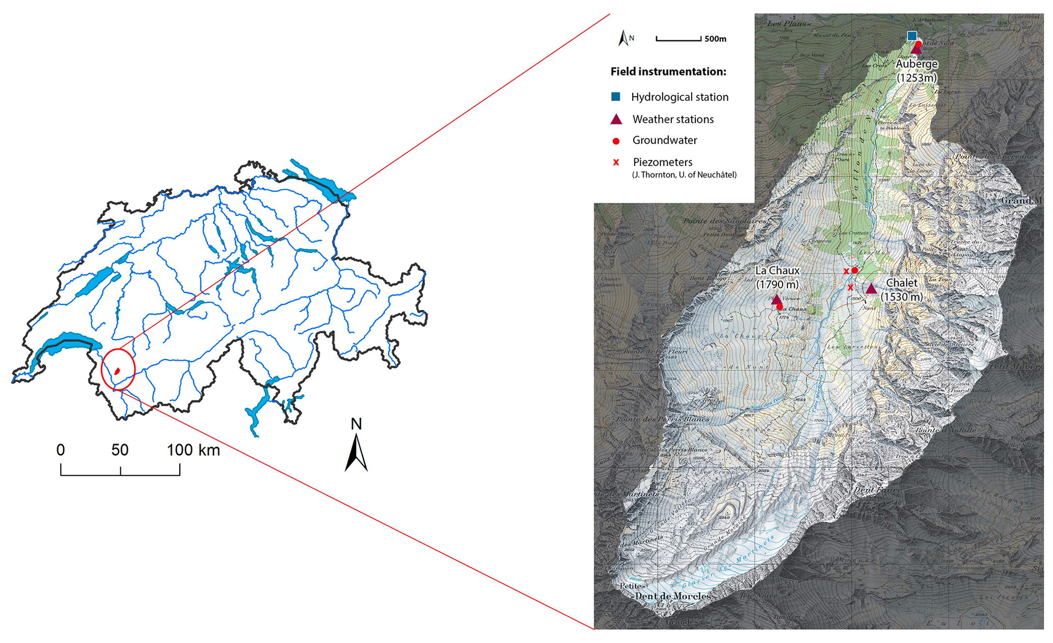
Figure 1 Map showing Vallon de Nant along with the locations of meteorologic and hydrologic observations as well as frequent sampling sites. Composite samples of precipitation were collected at the weather stations. Groundwater samples were collected at the groundwater monitoring points and the installed piezometers. The groundwater piezometers were installed by James Thornton from the University of Neuchâtel (Thornton et al., 2018).

3.4.2 Data collection

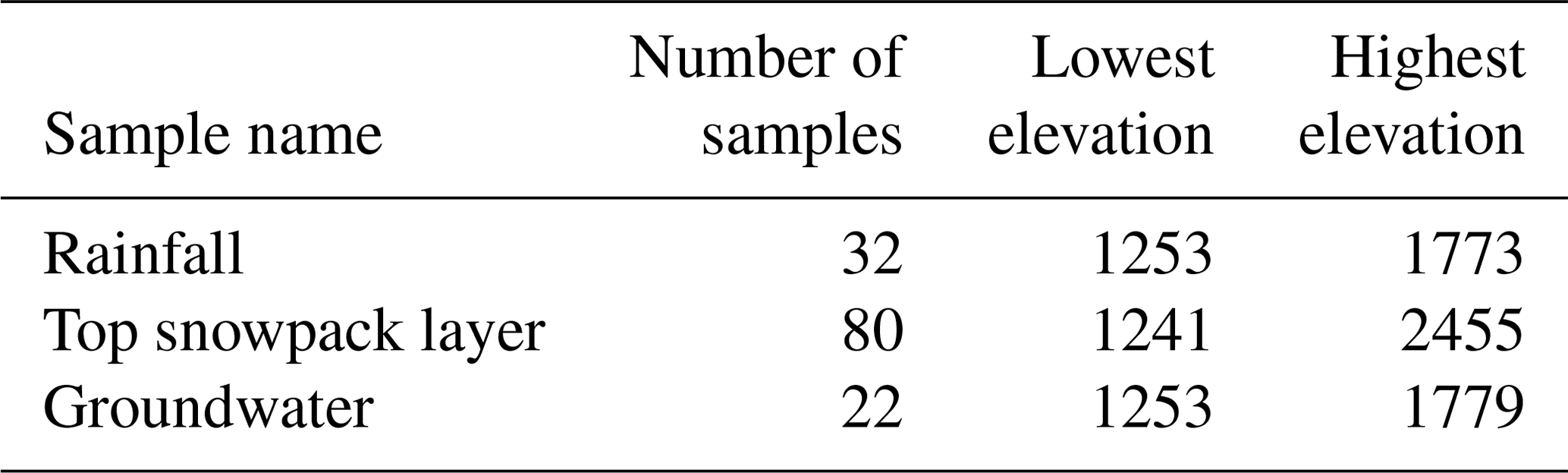
Vallon de Nant has been extensively monitored since February 2016. Water samples are collected from streamflow, rain, snowpack, and groundwater at different elevations, which are then analyzed for the isotopic ratios in deuterium (δ²H) and oxygen-18 (δ¹⁸O). Vallon de Nant is remotely located with very limited winter access, frequently experiencing winter avalanches. Due to these logistical constraints, snowmelt lysimeters or passive capillary samplers could not be set up to sample snowmelt water; accordingly, grab snowpack samples are used here as a proxy for snowmelt. A summary of the isotopic data is shown in Table  1.

Table 1 Summary of the isotopic data (δ²H and δ¹⁸O) collected in Vallon de Nant between February 2016 and July 2017.

3.4.3 Model implementation

HydroMix is used to estimate the proportion of snow recharging groundwater (subsequently referred to as the “snow recharge coefficient”). In order to obtain a PDF of the snow recharge coefficient, isotopic ratios in all the water samples from rain, snowpack, and groundwater are used. A uniform prior distribution is assigned to the snow recharge coefficient, which varies between 0 and 1, representing the entire range of possible values.

3.5 Introduction of an additional model parameter

In any mixing analysis, it may be useful or desirable for users to specify an additional model parameter that is able to modify the tracer concentrations based on their process understanding of the system. In the case of Alpine catchments with large elevation gradients, stable isotopes in precipitation often exhibit a systematic trend with elevation, becoming more depleted in heavier isotopes with increasing elevation. This is also known as the “isotopic lapse rate” (Dansgaard, 1964; Friedman et al., 1964). In typical field campaigns, because of logistical challenges, precipitation samples are collected only at a few points in a catchment, with often fewer precipitation samples at high elevations. This leads to oversampling at lower elevations and undersampling at higher elevations, which can bias mixing estimates. This has been found to be especially relevant for hydrograph separation in forested catchments (Cayuela et al., 2019). To allow a process compensation for this, an additional lapse rate factor is introduced with which each observed point-scale sample (observed at a given elevation) is corrected to a reference elevation as follows:

$$\begin{array}{}\text{(25)}& \stackrel{\mathrm{‾}}{r}={\displaystyle \frac{{\sum }_{j=\mathrm{1}}^k\left[\mathit{\alpha }\left(e_j-e\right)+r\right]a_j}{{\sum }_{j=\mathrm{1}}^k{a}_j}},\end{array}$$

where r is the isotopic ratio in precipitation collected at elevation e, $\stackrel{\mathrm{‾}}{r}$ is the catchment-averaged isotopic ratio in precipitation, α is the isotopic lapse rate factor, e_j is the elevation of the jth elevation band, and a_j is the catchment area under the jth elevation band; the catchment is divided into k elevation bands. These bands are obtained by constructing a hypsometric curve of the catchment (Strahler, 1952).

The lapse rate factor is allowed to modify both rainfall and snowpack isotopic ratios to obtain a catchment-averaged isotopic ratio, which is then used in the mixing model. Using this formulation of an isotopic lapse rate makes the following implicit assumptions: (1) precipitation storms on aggregate move from the lower part of the catchment to the upper part of the catchment, thus creating a lapse rate effect, and (2) precipitation falls uniformly over the catchment. It is important to note that the isotopic lapse rate is different from the precipitation lapse rate; i.e., the rate of change of precipitation with elevation is different from the rate of change of the precipitation isotopic ratio with elevation.

Figure 2 (a) Scatterplot showing the mixing ratio (ρ) values inferred using HydroMix for the low and high variance synthetic case in Table 3. The uncertainty band represents the inferred mixing ratio plus or minus the error standard deviation obtained from Eq. (13). The number of source and target samples is 100. (b) Performance of HydroMix in terms of the absolute error between the posterior mixing ratio mean and the true mean for the low variance dataset over all tested ratios plotted as a function of the number of samples drawn for the two sources.

Table 2 Prior distribution of the different model parameters as specified to HydroMix.

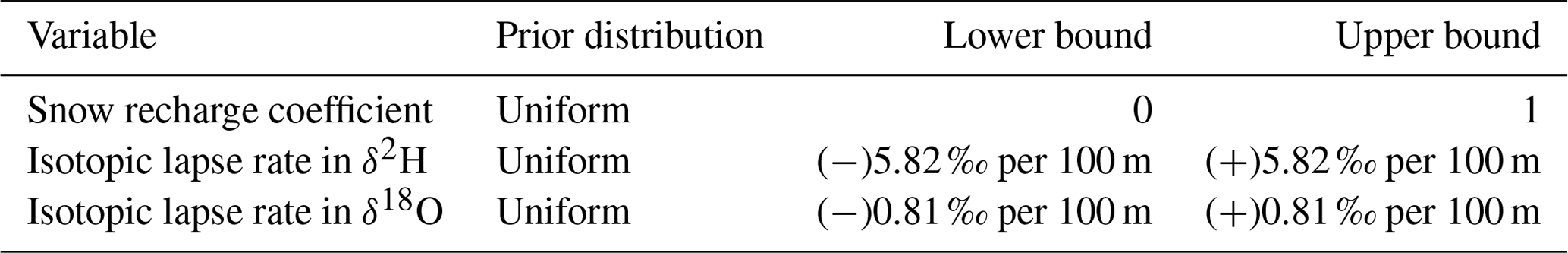
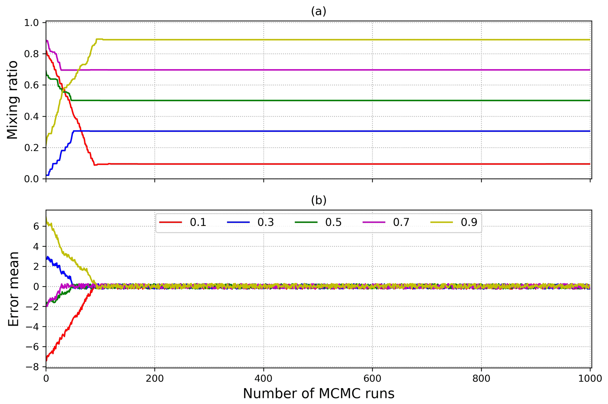
Figure 3 Diagnostic plots showing the convergence characteristics of MCMC chains for five different mixing ratios for the low variance dataset (shown in Table 3). Panels (a) and (b) show variations in the inferred mixing ratio and the error mean with increasing MCMC runs.

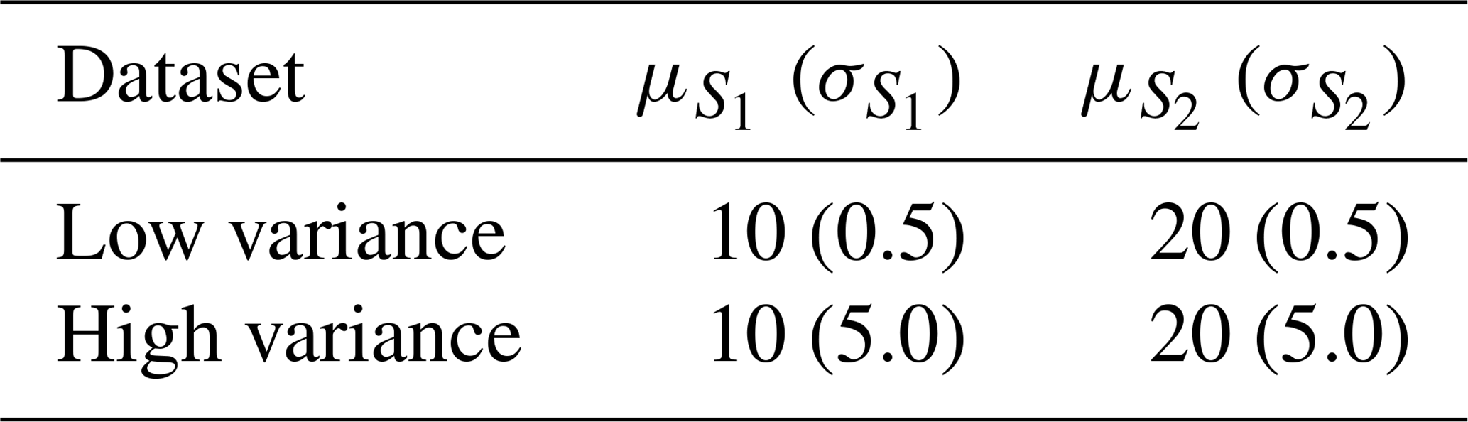
Table 3 Mean and variance of the two sources, S₁ and S₂, drawn from normal distributions.

It is important to note that the precipitation isotopic ratio is not only a function of elevation, but also depends on other factors such as the source of moisture origin, cloud condensation temperature, and secondary evaporation. Similarly, strong spatial variability exists in the isotopic ratio of snowmelt water, depending on catchment aspect, snow metamorphism, and wind distribution. This case study is a mere demonstration that HydroMix allows for the inference of additional parameters that can account for various physical processes that may modify isotopic ratios.

The prior distribution of the isotopic lapse rate is specified based on isotopic data collected across Switzerland under the Global Network of Isotopes in Precipitation (GNIP) program (IAEA/WMO, 2018). Using the monthly isotopic values collected between 1966 and 2014, average lapse rate values are obtained for both δ²H and δ¹⁸O. These were (−)1.94 ‰ per 100 m for δ²H and (−)0.27 ‰ per 100 m for δ¹⁸O (Beria et al., 2018).

A uniform prior distribution is assigned to the isotopic lapse rate parameter, with the lower bound specified as 3 times the Swiss lapse rate for both δ²H and δ¹⁸O. The observed isotopic lapse rate data from Switzerland suggest that average lapse rates are weakly negative; however, positive lapse rates can a priori not be excluded for the case study catchment. Accordingly, we do not specify an upper lapse rate bound of zero but set it as 3 times the Swiss lapse rate (Table 2). In the case of Vallon de Nant, the elevation ranges from 1253 m to 3051 m a.s.l. For computing the Swiss lapse rate, the elevation range over which the monthly precipitation samples were collected was 300 m to 2000 m a.s.l. This difference in elevation ranges between Vallon de Nant and the GNIP network should be kept in mind during the interpretation of results.

4 Results

The results for the different case studies are discussed in the sections below.

4.1 Mixing with normal distributions

The mean and standard deviations used to generate the low and high variance source distributions for the synthetic case studies are summarized in Table 3. We randomly generated 100 samples from each of the two source distributions and from the target distribution and varied the mixing ratios between 0.05 and 0.95 in 0.05 increments. It should be noted that HydroMix permits using a different number of samples for the sources and for the mixture.

For the low variance case, the mixing ratio inferred with HydroMix with 1000 MCMC simulations closely reproduces the theoretical mean of the mixing ratios used to generate the synthetic data (Fig. 2a). However, for the high variance case, the inferred mixing ratios do not match the true underlying mixing ratios, especially for low and high mixing ratios. This is partly due to the poor identifiability of the sources (given that their distributions are highly overlapping) and partly due to the relatively small sample size of 100. The inferred mean should reproduce the theoretical mean with increasing sample size and we clearly see this for the low variance case in Fig. 2b, where the model performance markedly improves with an increasing number of samples. The performance is measured here in terms of the absolute error between the posterior mixing ratio mean and the true mean summed and averaged over all tested ratios from 0.05 to 0.95. We did not perform inferences for sample sizes larger than 100 as the computational requirement increases exponentially with increasing sample sizes.

The model converges fairly quickly for the low variance case after ∼100 runs as shown in Fig. 3a. The obtained model residuals have zero mean and are approximatively normally distributed as revealed by quantile–quantile plots (not shown), in line with the assumption of an unbiased normally distributed error model, as stated in Eq. (7).

4.2 Contribution of rain and snow to groundwater recharge using a hydrologic model

Figure 4 shows the variation in the isotopic ratio of groundwater over the entire 100-year period, showing that the system achieves a steady-state condition after ∼15 years of simulation. The mixing ratio is estimated with HydroMix using (1) samples of the isotopic ratio in snowfall and (2) samples of the isotopic ratio in snowmelt. The two sample distributions differ, as shown in Fig. 5, where the variability of the isotopic ratio is lower in snowmelt when compared to snowfall. In the model at hand, this reduction is obtained because of mixing occurring within the snowpack, leading to homogenization and thus reducing the variability in the isotopic ratio of snowmelt. In field data, such a reduction in variability is also generally observed (Beria et al., 2018) as a result of the homogenization as modeled here and from more complex snow physical processes, which lie beyond the scope of this study.

Table 4 Parameters used to generate time series of precipitation, air temperature, and isotopic ratios in precipitation. μ represents the mean, A is the amplitude, and φ is the time lag of the underlying sine function. For the precipitation process, μ is the mean intensity on days with precipitation. The resulting mean winter length (air temperature below 0 ^∘C) is 119.5 d.

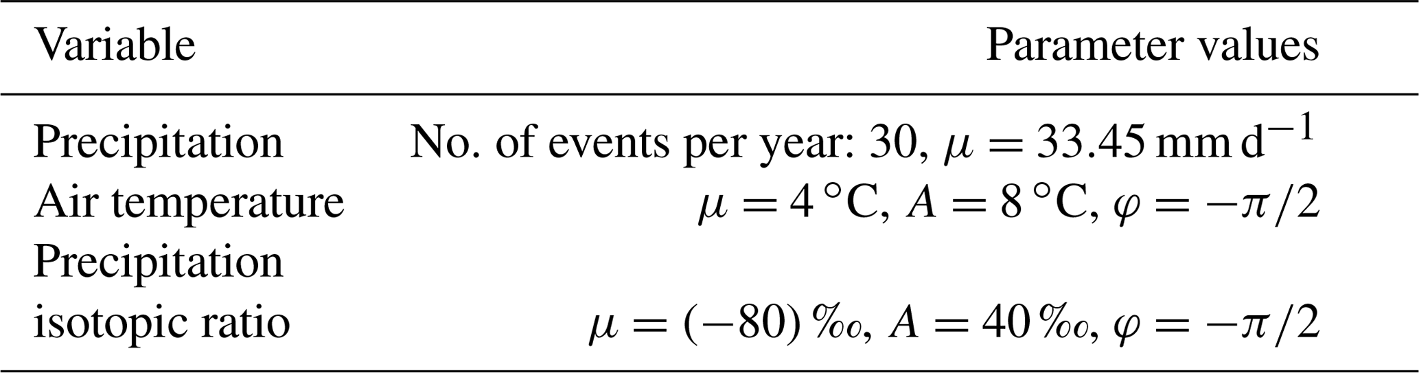
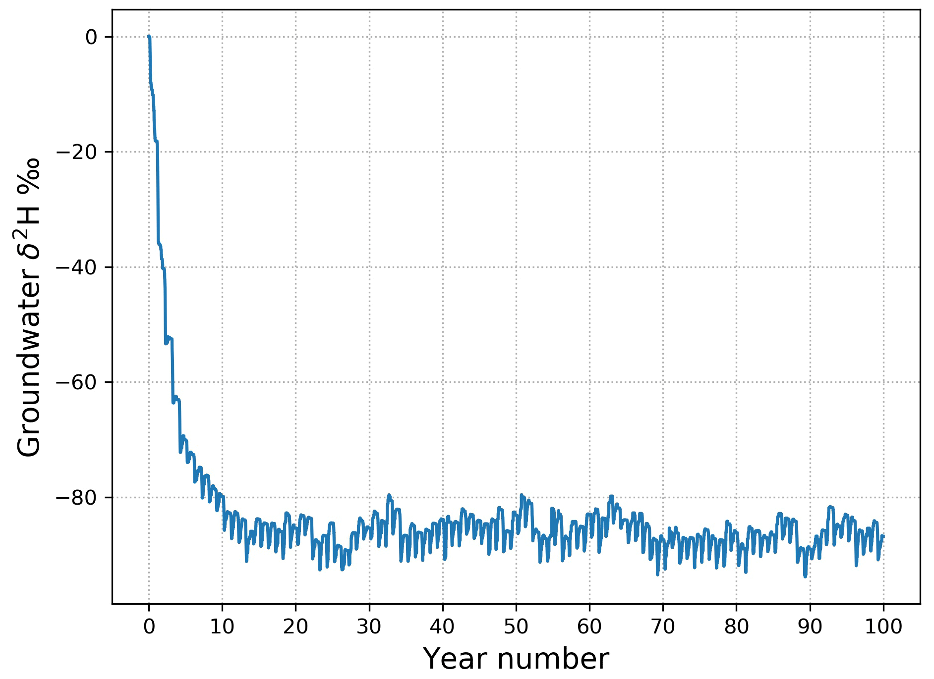
Figure 4 Evolution of the modeled isotopic ratio in groundwater over a 100-year period with R_r=0.3 and R_s=0.6.

The mixing ratios inferred with HydroMix are very similar regardless of whether snowfall or snowmelt is used across the entire range of recharge efficiencies (Fig. 6). This provides confidence in the use of snowfall samples as a proxy for snowmelt when estimating mixing ratios. However, it is clear from Fig. 6 that an important bias emerges between the estimated mixing ratio from HydroMix and the actual mixing ratio known from the hydrologic model, especially for low mixing ratios.

This bias can be expected to emerge when the source contributions are not weighted according to their fluxes, which to our knowledge has not been explicitly addressed in the hydrological literature. As already discussed in Sect. 3.3, the absence of sample weighting typically induces a bias when there is a large divergence between the number of samples taken over a certain period (e.g., 1 year) to characterize a source and the magnitude of source flux over that period (e.g., 40 snow and 10 rain samples taken to characterize the two sources, for which snow only accounts for a very small portion, e.g., 10 %, of the annual precipitation).

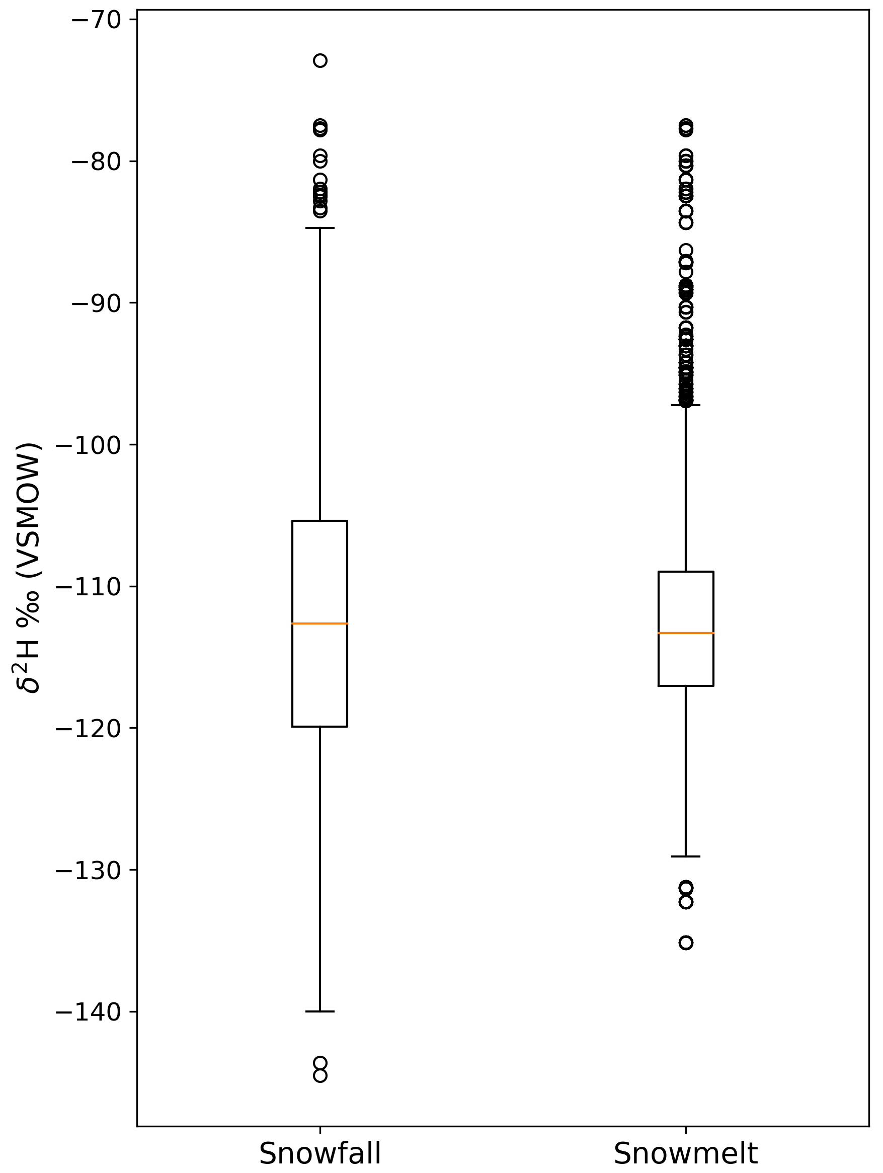
Figure 5 Box plot showing the variability in the isotopic ratio of snowfall and snowmelt as simulated by the hydrologic model. The box plot extends from the 25th to 75th percentile value, with the median value depicted by the orange line. The whiskers extend up to 1.5 times the interquartile range. The black circles are the outliers.

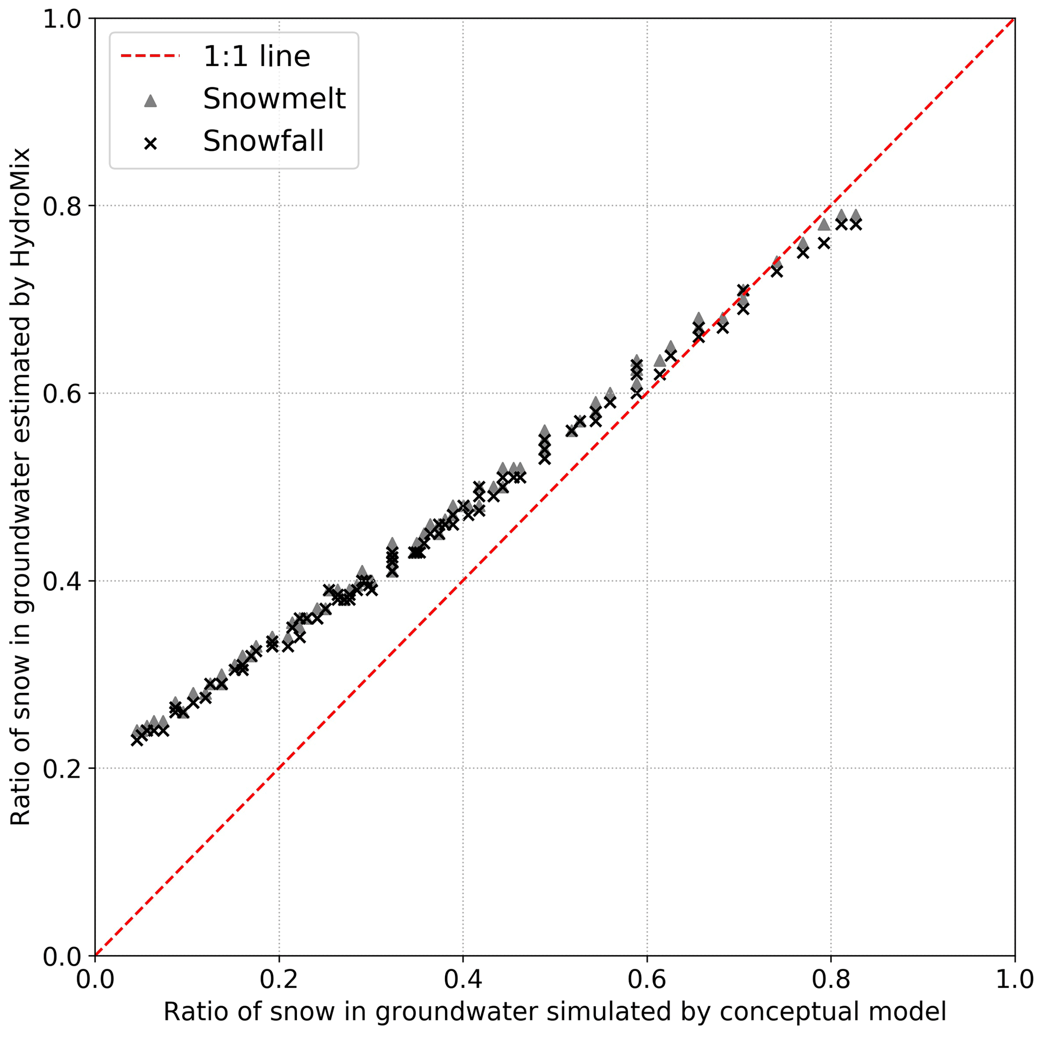
Figure 6 Ratios of snow in groundwater estimated with HydroMix plotted against ratios obtained from the hydrologic model for the last 2 years of simulation. Also shown are the separate results obtained by using samples of either snowmelt or snowfall. The full range of ratios is obtained by varying rainfall and snowmelt recharge efficiencies from 0.05 to 0.95. The numbers of rainfall, snowfall, and snowmelt days are 39, 24, and 107 in the last 2 years of simulation.

4.3 Effect of weights on estimates of mixing ratios using a hydrologic model

After taking into account the magnitude of rainfall and snowmelt events in the composite likelihood function of Eq. (23), it is clear that many of the unweighted biases can be removed (Fig. 7). The most significant improvement is seen at very low mixing ratios for which the divergence between the conceptual model and the mixing model estimates error is reduced by almost 50 %. In this study, we have used a relatively simple normalization-based weighting function (Eq. 25). Testing other weighting functions that have been proposed in the past (Vasdekis et al., 2014) is left for future research.

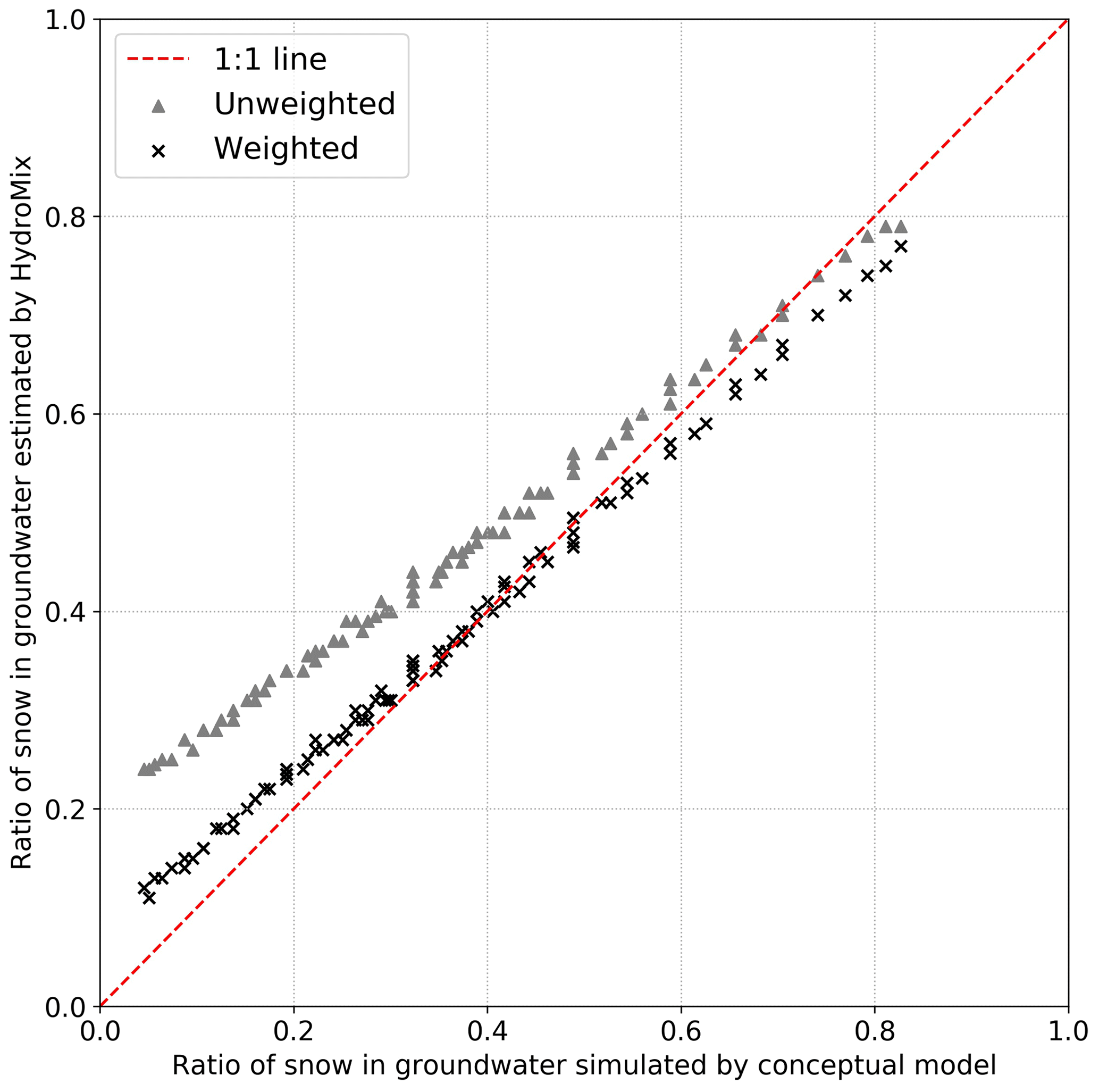
Figure 7 Ratios of snow in groundwater estimated using HydroMix plotted against ratios obtained from the hydrologic model for both weighted and unweighted mixing scenarios. The full range of ratios is obtained by varying rainfall and snowmelt recharge efficiencies from 0.05 to 0.95. The numbers of rainfall, snowfall, and snowmelt days are 39, 24, and 107 in the last 2 years of simulation.

4.4 Inferring fraction of snow recharging groundwater in a small Alpine catchment along with an additional model parameter

Using the dataset from an Alpine catchment (Vallon de Nant, Switzerland), HydroMix estimates that 60 %–62 % of the groundwater is recharged from snowmelt (using unweighted approach), with the full posterior distributions shown in Fig. 8a. This estimate is consistent for both of the isotopic tracers (δ²H and δ¹⁸O), which are often used interchangeably in the hydrologic literature (Gat, 1996). Comparing this recharge estimate to the proportion of total precipitation that falls as snow (around 40 %–45 %; see Sect. 3.4.1) suggests that snowmelt is more effective at reaching the aquifer than an equivalent amount of rainfall falling at a different period of the year. Similar results have been obtained in a number of previous studies across the temperate and mountainous regions of the world (see Table 1 in the work of Beria et al., 2018, for a summary).

Figure 8 Histogram showing the fraction of snow recharging groundwater in Vallon de Nant using the isotopic ratios in δ²H and δ¹⁸O (a) without correcting for lapse rate and (b) after correcting for lapse rate.

As can be seen from Fig. 8a, the estimated distribution of the snow ratio in groundwater is very narrow. This can be explained by the fact that we assume that the collected precipitation samples represent the variability actually occurring in the catchment. To overcome this limitation, we infer an additional parameter called the isotopic lapse rate that accounts for the spatial heterogeneity in terms of catchment elevation. As shown in Fig. 9, the posterior distributions of the isotopic lapse rate (for both δ²H and δ¹⁸O) largely overlap the spatially averaged isotopic lapse rate as estimated from precipitation isotopes across Switzerland. The overlap with the average Swiss isotope lapse rate suggests that our inferred lapse rates are reasonable, with the spread in the estimates likely reflecting the temporal variation in the catchment-specific isotope lapse rate that can develop from a wide range of moderating factors (e.g., air masses contributing precipitation without traversing the full elevation range of the catchment due to varying trajectories). The Swiss lapse rate is constructed as a long-term spatial average, whereas the inferred isotopic lapse rate in Vallon de Nant is constructed from the temporal variations in the isotopic ratios. These results demonstrate that it is relatively straightforward to jointly infer multiple parameters within the HydroMix modeling framework.

However, an important consequence of additional parameter inference without providing additional data or constraints is an increase in the degree of freedom, which can then increase the uncertainty in source contributions. This effect is seen in Fig. 8b, especially in contrast with the previous result in Fig. 8a, where the median mixing ratios of the posterior distributions remain similar (∼0.6), but the spread increases drastically from 0.005 to 0.2.

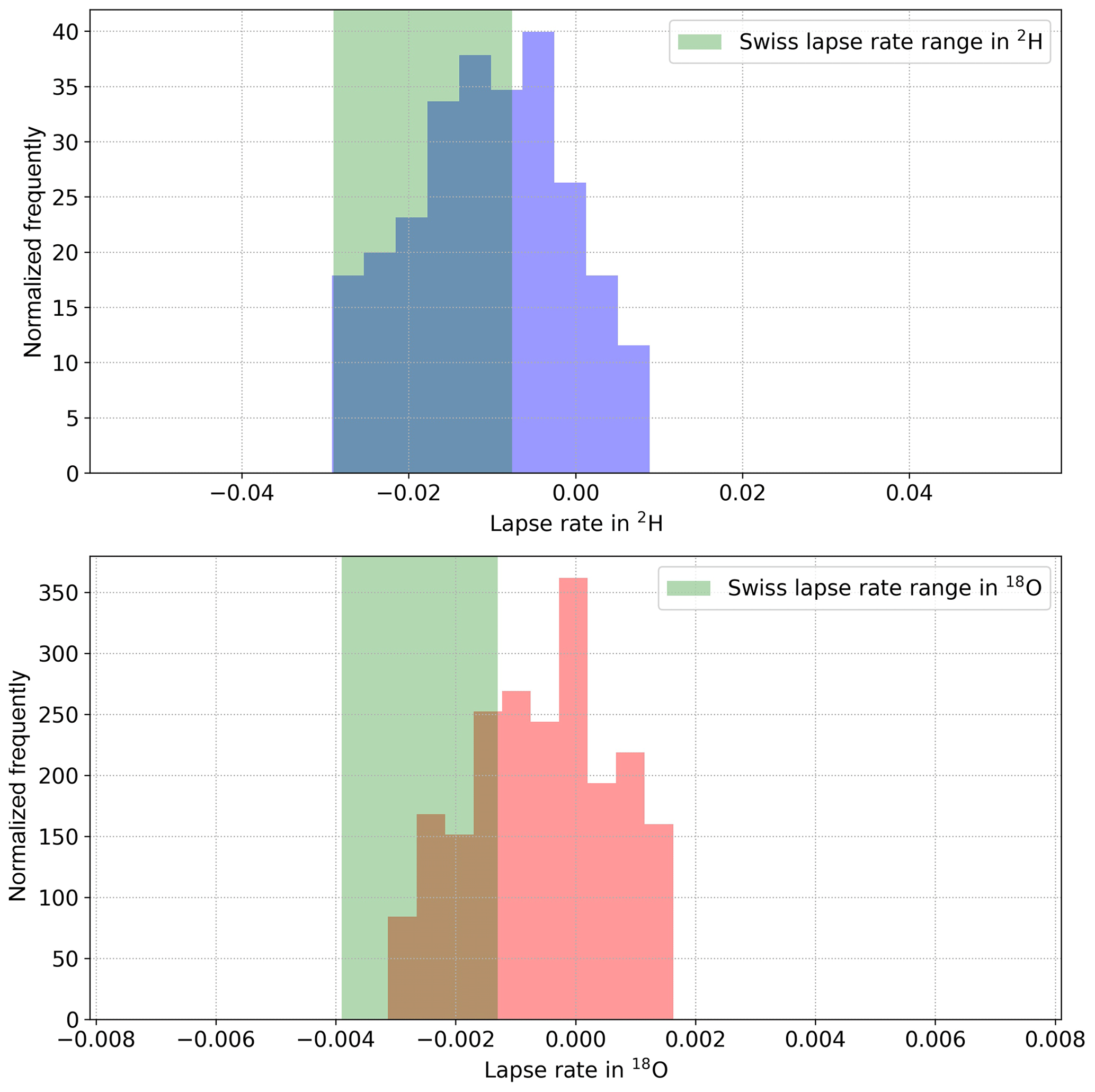
Figure 9 Histogram showing the posterior distribution of the isotope lapse rate parameter in δ²H and δ¹⁸O. The green region shows the confidence bounds (significant at α=0.01) of the lapse rate computed over Switzerland by using inverse variance-weighted regression. The limits of the prior distribution of the isotopic lapse rates correspond to the limits of the x axis. The slope of the isotopic ratio when plotted against elevation for the Swiss-wide data is shown in Fig. 3 of Beria et al. (2018).

5 Limitations and opportunities

As with all linear mixing models, the quality of the underlying data determines the accuracy and utility of the results. If the tracer compositions of the different sources are not sufficiently distinct, the uncertainty in the estimated mixing ratios will become very large. This means that if either the underlying data quality is poor or the source contribution dynamics are not well conceptualized, then the uncertainty in the mixing ratios will be too high to be useful.

In cases in which a large number of source samples are available, the computational requirements of HydroMix outweigh the benefit from using it. These are likely cases in which the statistical distribution of the source tracer composition is well understood, and therefore fitting a probability density curve to the source and target samples and then inferring the distribution of the mixing ratio using a probabilistic programming approach is more appropriate (Carpenter et al., 2017; Parnell et al., 2010; Stock et al., 2018). Also, HydroMix might not be an appropriate method in instances in which fitting statistical distributions to source and target compositions reflects a priori knowledge of the system.

A key difference between HydroMix and other Bayesian mixing approaches is that HydroMix parameterizes the error function, whereas other Bayesian approaches parameterize the statistical distribution of source and mixture compositions. Parameterizing source compositions requires large sample sizes, which is seldom the case in tracer hydrology. Error parameterization offers a useful alternative and can also be verified against the posterior error distribution. In the case studies demonstrated in this paper, a normally distributed error model was found to be appropriate. However, error models other than Gaussian can be used by formulating the respective likelihood function.

HydroMix builds the model residuals by comparing all the observed source samples with all the observed samples of the target mixture, assuming that all available source and target samples are independent. Interestingly, the assumption of independence holds even if the source and target samples are taken at the same time, since the target samples result from water that has traveled for a certain amount of time in the catchment and hence is not related to the water entering the catchment. However, if a system has instantaneous mixing, then the source and target samples taken at the same moment in time will necessarily be strongly correlated. In such cases, the assumption of independent samples would not make sense and the method might give spurious results.

Finally, it is noteworthy that adding additional parameters to characterize the source tracer composition increases the degree of freedom of the model, which implies that adding such parameters leads to an increase in the uncertainty of the source contribution estimates unless new information, i.e., new observed data, is added to the model. This means that users who are interested in incorporating additional modification processes by adding parameters should ideally provide additional tracer data able to constrain this process, subject to tracer data being available.

For consistency and simplicity, the case studies and synthetic hydrological examples provided here focused on the contribution of rain and snow in recharging groundwater. However, it is important to emphasize that the opportunities to implement HydroMix extend to all cases in which mixing contributions are of interest and for which it is difficult to build extensive databases of source tracer compositions. Such examples include quantifying the amount of “pre-event” vs. “event” water in streamflow; pre-event water refers to groundwater and event water refers to rainfall or snowmelt. Another interesting use case might be to quantify the proportion of streamflow coming from the different source areas in a catchment to capture the spatial dynamics of streamflow. Other uses include quantifying the amount of fog contributing to throughfall, the proportion of glacial melt vs. snowmelt flowing into a stream, the amount of vegetation water use from soil moisture at different depths vs. groundwater, the interaction between surface water and groundwater at the hyporheic zone (Leslie et al., 2017), and sediment fingerprinting to quantify the spatial origin of river sediments. In all of these cases, understanding source water contributions, both spatially and temporally, will improve the physical understanding of the system.

6 Conclusions

We develop a new Bayesian modeling framework for the application of tracers in mixing models. The primary application target of this framework is hydrology, but it is by no means limited to this field. HydroMix formulates the linear mixing problem in a Bayesian inference framework that infers the model parameters with a Metropolis–Hastings-based MCMC sampling algorithm based on differences between observed and modeled tracer concentrations in the target mixture using all possible combinations between all source and target concentration samples. This is especially useful in data-scarce environments where fitting probability distribution functions is not feasible. HydroMix also makes the inclusion of additional model parameters to account for source modification processes straightforward. Examples include known spatial or temporal tracer variations (e.g., isotopic lapse rates or evaporative enrichment).

An evaluation of HydroMix with data from different synthetic and field case studies leads to the following conclusions.

1. HydroMix gives reliable results for mixing applications with small sample sizes (<20–30 samples). As expected, the variance in source tracer composition and the ensuing composition overlap determines the bias in the mixing ratio estimates. The bias in mixing ratio estimates increases with increasing variance in source tracer compositions. Mixing ratio estimates improve (in terms of lower error) with an increasing number of source samples.

2. As revealed by our synthetic case study with a conceptual hydrological model, at low source contributions (i.e., <20 %), a strong divergence between the actual and estimated mixing ratios emerges. This arises if HydroMix assigns equal weights to all source samples by proportionally oversampling the less abundant source, which then leads to significant biases in mixing estimates. This problem is inherent to all mixing approaches and to our knowledge has not been adequately addressed in the literature.

3. The use of composite likelihoods to weight samples by their amounts can significantly reduce the bias in the mixing estimates. At low source proportions, the estimated mixing ratio improves by more than 50 % after accounting for the amount of all the sources. We show this using a simple normalization-based weighting function. Future studies should explore the usage of different weighting functions that have been proposed in the past (Vasdekis et al., 2014).

4. A synthetic application of HydroMix to understand the amount of snowmelt-induced groundwater recharge revealed that using the snowfall isotopic ratio instead of the snowmelt isotopic ratio leads to similar mixing ratio estimates. This is particularly useful in high mountainous catchments, where sampling snowmelt is logistically difficult.

5. A real case application of HydroMix in a Swiss Alpine catchment (Vallon de Nant) showed a clear winter bias in groundwater recharge. About 60 %–62 % of the groundwater is recharged from snowmelt (unweighted mixing approach), while snowfall only accounts for 40 %–45 % of the total annual precipitation. This has also been previously suggested elsewhere in the European Alps (Cervi et al., 2015; Penna et al., 2014, 2017; Zappa et al., 2015).

To conclude, HydroMix provides a Bayesian approach to mixing model problems in hydrology that takes full advantage of small sample sizes. Future work will show the full potential of this approach in hydrology as well as other environmental modeling applications.

Appendix A

The equations below show the numerical implementation of the evolution of isotopic ratios in snowpack, isotopic ratios in groundwater, and groundwater storage at a daily time step.

$$\begin{array}{}\text{(A1)}& C_{\mathrm{s}}\left(t\right)={\displaystyle \frac{C_{\mathrm{s}}\left(t-\mathrm{1}\right)h_{\mathrm{s}}\left(t-\mathrm{1}\right)+C_{\mathrm{p}}\left(t\right)P_{\mathrm{s}}\left(t\right)-C_{\mathrm{s}}\left(t-\mathrm{1}\right)M_{\mathrm{s}}\left(t\right)}{h_{\mathrm{s}}\left(t-\mathrm{1}\right)+P_{\mathrm{s}}\left(t\right)-M_{\mathrm{s}}\left(t\right)}}\end{array}$$

$$\begin{array}{}\text{(A2)}& C_{\mathrm{g}}\left(t\right)={\displaystyle \frac{{\displaystyle \begin{array}{c}{C}_{\mathrm{g}}\left(t-\mathrm{1}\right)G\left(t-\mathrm{1}\right)+C_{\mathrm{p}}\left(t\right)R_{\mathrm{r}}{P}_{\mathrm{r}}\left(t\right)\\ +C_{\mathrm{s}}\left(t\right)R_{\mathrm{s}}{M}_{\mathrm{s}}\left(t\right)-C_{\mathrm{g}}\left(t-\mathrm{1}\right)Q\left(t\right)\end{array}}}{\begin{array}{c}G\left(t-\mathrm{1}\right)+R_{\mathrm{r}}{P}_{\mathrm{r}}\left(t\right)\\ +R_{\mathrm{s}}{M}_{\mathrm{s}}\left(t\right)-Q\left(t\right)\end{array}}}\end{array}$$

$$\begin{array}{}\text{(A3)}& G\left(t\right)=G\left(t-\mathrm{1}\right)+R_{\mathrm{r}}{P}_{\mathrm{r}}\left(t\right)+R_{\mathrm{s}}{M}_{\mathrm{s}}\left(t\right)-k(G\left(t\right)-G_{\mathrm{C}})\end{array}$$