the Creative Commons Attribution 4.0 License.
the Creative Commons Attribution 4.0 License.
 | 18 May 2020
The GGCMI Phase 2 experiment: global gridded crop model simulations under uniform changes in CO2, temperature, water, and nitrogen levels (protocol version 1.0)
James A. Franke
Joshua Elliott
Alex C. Ruane
Jonas Jägermeyr
Juraj Balkovic
Philippe Ciais
Marie Dury
Pete D. Falloon
Christian Folberth
Louis François
Tobias Hank
Munir Hoffmann
R. Cesar Izaurralde
Ingrid Jacquemin
Curtis Jones
Nikolay Khabarov
Marian Koch
Michelle Li
Wenfeng Liu
Stefan Olin
Meridel Phillips
Thomas A. M. Pugh
Ashwan Reddy
Xuhui Wang
Karina Williams
Florian Zabel
Elisabeth J. Moyer
Concerns about food security under climate change motivate efforts to better understand future changes in crop yields. Process-based crop models, which represent plant physiological and soil processes, are necessary tools for this purpose since they allow representing future climate and management conditions not sampled in the historical record and new locations to which cultivation may shift. However, process-based crop models differ in many critical details, and their responses to different interacting factors remain only poorly understood. The Global Gridded Crop Model Intercomparison (GGCMI) Phase 2 experiment, an activity of the Agricultural Model Intercomparison and Improvement Project (AgMIP), is designed to provide a systematic parameter sweep focused on climate change factors and their interaction with overall soil fertility, to allow both evaluating model behavior and emulating model responses in impact assessment tools. In this paper we describe the GGCMI Phase 2 experimental protocol and its simulation data archive. A total of 12 crop models simulate five crops with systematic uniform perturbations of historical climate, varying CO2, temperature, water supply, and applied nitrogen (“CTWN”) for rainfed and irrigated agriculture, and a second set of simulations represents a type of adaptation by allowing the adjustment of growing season length. We present some crop yield results to illustrate general characteristics of the simulations and potential uses of the GGCMI Phase 2 archive. For example, in cases without adaptation, modeled yields show robust decreases to warmer temperatures in almost all regions, with a nonlinear dependence that means yields in warmer baseline locations have greater temperature sensitivity. Inter-model uncertainty is qualitatively similar across all the four input dimensions but is largest in high-latitude regions where crops may be grown in the future.
- Article
(9803 KB) - Full-text XML
- Companion paper
-
Supplement
(19844 KB) - BibTeX
- EndNote


Understanding crop yield response to a changing climate is critically important, especially as the global food production system will face pressure from increased demand over the next century (Foley et al., 2005; Bodirsky et al., 2015). Climate-related reductions in supply could therefore have severe socioeconomic consequences (e.g., Stevanović et al., 2016; Wiebe et al., 2015). Multiple studies using different crop or climate models concur in projecting sharp yield reductions on currently cultivated cropland under business-as-usual climate scenarios, although their yield projections show considerable spread (e.g., Rosenzweig et al., 2014; Schauberger et al., 2017; Porter et al., 2014, and references therein). Although forecasts of future yields reductions can be made with simple statistical models based on regressions in historical weather data, process-based models, which simulate the effect of temperature, water and nutrient availability, and atmospheric CO2 concentration on the process of photosynthesis and the biology and phenology of individual crops, play a critical role in assessing the impacts of climate change.
Process-based models are necessary for understanding crop yields in novel conditions not included in historical data, including higher CO2 levels, out-of-sample combinations of rainfall and temperature, cultivation in areas where crops are not currently grown, and differing management practices (e.g., Pugh et al., 2016; Roberts et al., 2017; Minoli et al., 2019). Process-based models have therefore been widely used in studies on future food security (Wheeler and Von Braun, 2013; Elliott et al., 2014a; Frieler et al., 2017), options for climate mitigation (Müller et al., 2015) and adaptation (Challinor et al., 2018), and future sustainable development (Humpenöder et al., 2018; Jägermeyr et al., 2017). They are a necessity for global gridded simulations, which allow understanding the global dynamics of agricultural trade, because global market mechanisms can strongly modulate the economic impacts of regional yield changes (Stevanović et al., 2016; Hasegawa et al., 2018). Global simulations are especially necessary in studying agricultural effects of climate change (Müller et al., 2017), since systematic climate assessments must account for cultivation area changes and crop selection switching (Rosenzweig et al., 2018; Ruane et al., 2018) and must consider inter-regional differences (e.g., Nelson et al., 2014; Wiebe et al., 2015).
Modeling crop responses, however, continues to be challenging, as crop growth is a function of complex interactions between climate inputs, soil, and management practices (Boote et al., 2013; Rötter et al., 2011). Models tend to agree broadly in major response patterns, including a reasonable representation of the spatial pattern in historical yields of major crops and projections of shifts in yield under future climate scenarios (e.g., Elliott et al., 2015; Müller et al., 2017). But process-based models still struggle with some important details, including reproducing historical year-to-year variability in many regions (e.g., Müller et al., 2017; Jägermeyr and Frieler, 2018), reproducing historical yields when driven by reanalysis weather (e.g., Glotter et al., 2014), and low sensitivity to extreme events (e.g., Glotter et al., 2015; Schewe et al., 2019). Global models pose additional challenges due to variable input data quality and limited ability for model calibration. Long-term projections therefore retain considerable uncertainty (Wolf and Oijen, 2002; Jagtap and Jones, 2002; Iizumi et al., 2010; Angulo et al., 2013; Asseng et al., 2013, 2015).
Model intercomparison projects such as the Agricultural Model Intercomparison and Improvement Project (AgMIP; Rosenzweig et al., 2013) are crucial in quantifying uncertainties in model projections (Rosenzweig et al., 2014). Intercomparison projects have also been used to develop protocols for evaluating overall model performance (Elliott et al., 2015; Müller et al., 2017) and to assess the representation of individual physical mechanisms such as water stress and CO2 fertilization (e.g., Schauberger et al., 2017). However, to date, few such projects have systematically sampled critical factors that may interact strongly in affecting crop yields. A number of modeling exercises in the last 5 years have begun to use systematic parameter sweeps in crop model evaluation and emulation (e.g., Ruane et al., 2014; Makowski et al., 2015; Pirttioja et al., 2015; Fronzek et al., 2018; Snyder et al., 2019; Ruiz-Ramos et al., 2018), but all involve limited sites and most also limited crops and scenarios.
The Global Gridded Crop Model Intercomparison (GGCMI) Phase 2 experiment is the first global gridded crop model intercomparison involving a systematic parameter sweep across critical interacting factors. GGCMI Phase 2 is an activity of AgMIP, and a continuation of a multi-model comparison exercise begun in 2014. The initial GGCMI Phase 1 (Elliott et al., 2015; Müller et al., 2017) compared harmonized yield simulations over the historical period, with primary goals of model evaluation and understanding sources of uncertainty (including model parameterization, weather inputs, and cultivation areas); see also Folberth et al. (2019) and Porwollik et al. (2017) for more information. GGCMI Phase 2 compares simulations across a set of inputs with uniform perturbations to historical climatology, including CO2, temperature, precipitation, and applied nitrogen, as well as adaptation to shifting growing seasons (collectively referred to as “CTWN-A”). The CTWN-A experiment is inspired by AgMIP's Coordinated Climate-Crop Modeling Project (C3MP; see Ruane et al., 2014; McDermid et al., 2015) and contributes to the AgMIP Coordinated Global and Regional Assessments (CGRA; see Ruane et al., 2018; Rosenzweig et al., 2018).
In this paper, we describe the GGCMI Phase 2 model experiments and present initial summary results. In the sections that follow, we describe the experimental goals and protocols; the different process-based models included in the intercomparison; the levels of participation by the individual models. We then provide an assessment of model fidelity based on observed yields at the country level, and show some selected examples of the simulation output dataset to illustrate model responses across the input dimensions.
2.1 Goals
The guiding scientific rationale of GGCMI Phase 2 is to provide a comprehensive, systematic evaluation of the response of process-based crop models to critical interacting factors, including CO2, temperature, water, and applied nitrogen under two contrasting assumptions on growing season adaptation (CTWN-A). The dataset is designed to allow researchers to
-
enhance understanding of models sensitivity to climate and nitrogen drivers;
-
study the interactions between climate variables and nitrogen inputs in driving modeled yield impacts;
-
characterize differences in crop responses to climate change across the Earth's climate regions;
-
provide a dataset that allows statistical emulation of crop model responses for downstream modelers; and
-
explore the potential effects on future yield changes of adaptations in growing season length.
2.2 Modeling protocol
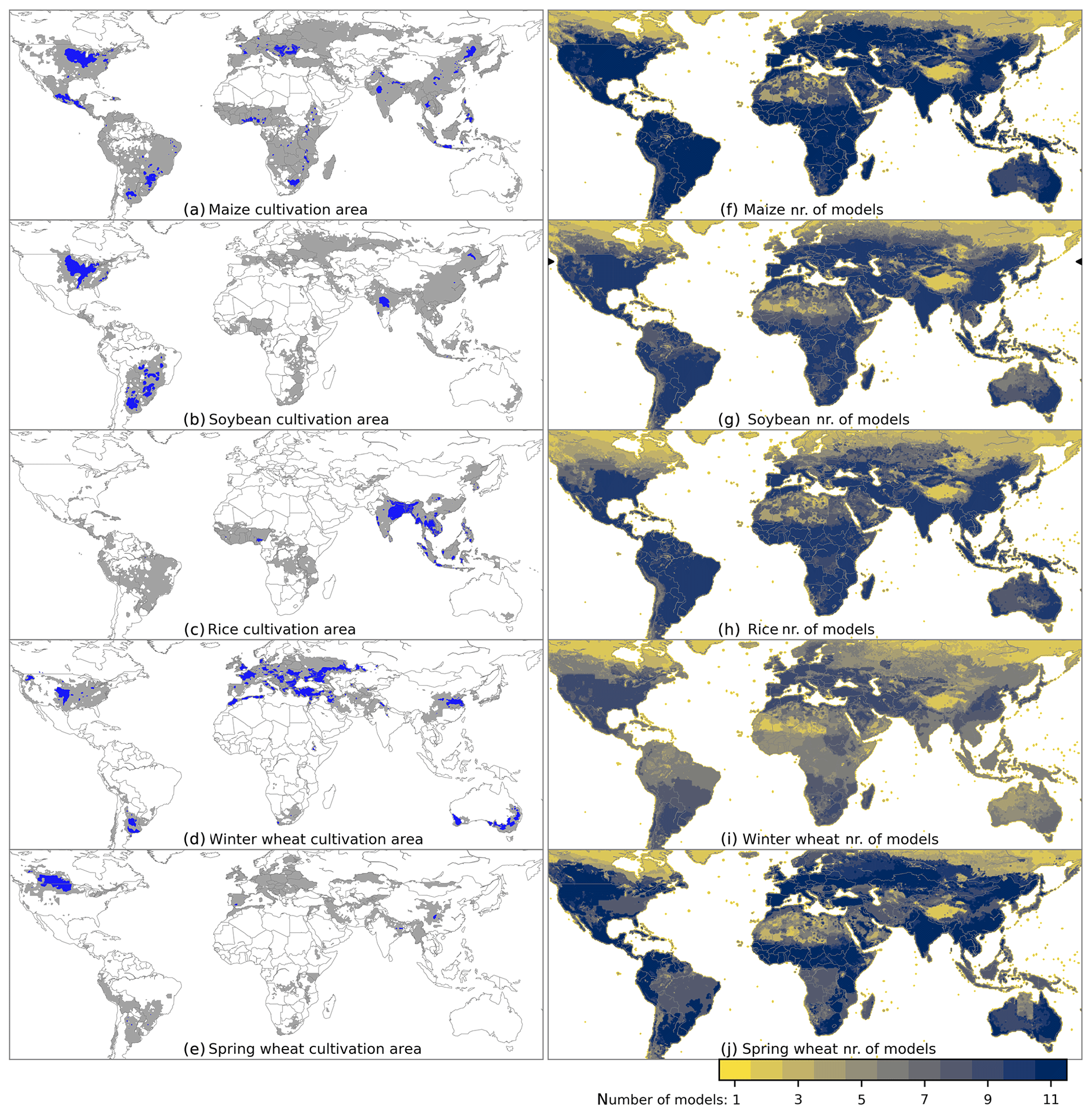
Figure 1(a–e) Cultivated areas for maize, rice, and soybean from the MIRCA2000 (Monthly Irrigated and Rainfed Crop Areas around the year 2000) dataset (Portmann et al., 2010). Blue indicates grid cells with more that 20 000 ha (10 % of the equatorial grid cell), and the gray contour shows grid cells with more that 10 ha cultivated. Areas for winter and spring wheat areas are adapted from MIRCA2000 and two other sources; see text for details. For irrigated crops, see Fig. S1 in the Supplement. (f–j) Number of models providing simulations for each grid cell. All models provide the minimum areal coverage of the GGCMI Phase 2 protocol, but some provide extra coverage at high latitudes or in arid or otherwise unsuitable areas.
The GGCMI Phase 1 intercomparison was a relatively limited computational exercise, requiring yield simulations for 19 crops across a total of 310 model years of historical scenarios, and had the participation of 14 modeling groups. The GGCMI Phase 2 protocol is substantially larger, involving over 1400 individual 30-year global scenarios, or over 42 000 model years; 12 modeling groups nevertheless participated. To reduce the computational load, the GGCMI Phase 2 protocol reduces the number crops to five (maize, rice, soybean, spring wheat, and winter wheat). The reduced set of crops includes the three major global cereals and the major legume and accounts for over 50 % of human calories in 2016: nearly 3.5 billion tons or 32 % of total global crop production by weight (FAO, 2018). This set of major crops has the advantage of historical yield data globally available at subnational scale (Ray et al., 2012; Iizumi et al., 2014), and has been frequently used in subsequent analyses (e.g., Müller et al., 2017; Porwollik et al., 2017).
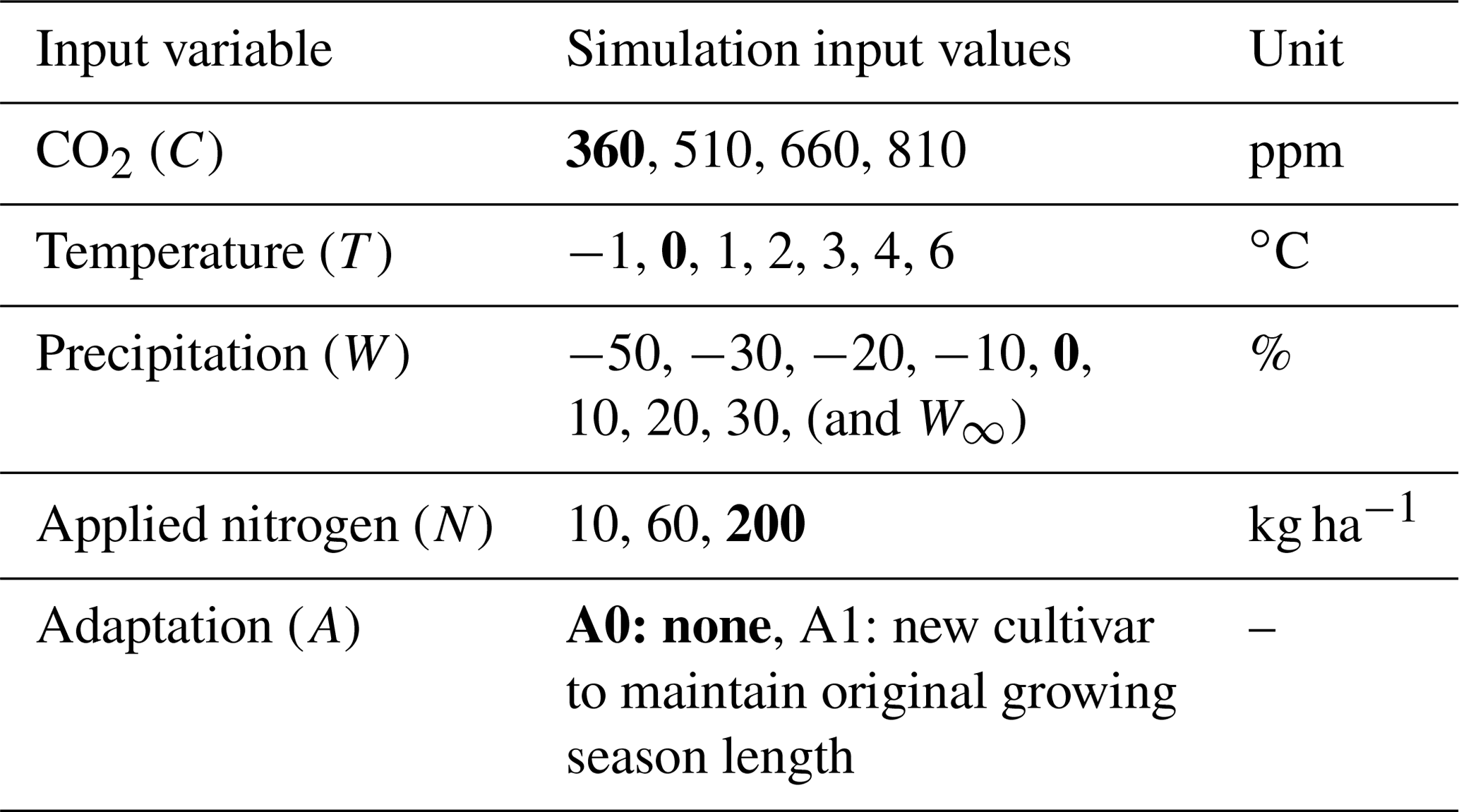
The Phase 2 protocol involves a suite of uniform perturbations from a historical climate time series. The baseline climate scenario for GGCMI Phase 2 is one of the weather products used in Phase 1, daily climate inputs for 1980–2010 from the 0.5∘ NASA AgMERRA (“agricultural”-modified Modern Era Retrospective analysis for Research and Applications) gridded reanalysis product. AgMERRA is specifically designed for agricultural modeling, with satellite-corrected precipitation (Ruane et al., 2015). The experimental protocol consists of 9 levels for water supply perturbations, 7 for temperature, 4 for CO2, and 3 for applied nitrogen, for a total of 756 simulations (Table 1), 672 for rainfed agriculture and an additional 84 for irrigated (W∞). Values of climate variable perturbations are selected to represent reasonable ranges for changes over the medium term (to 2100) under business-as-usual emissions. Values for nitrogen application levels are intended to cover a wide range of potentials. The resulting GGCMI Phase 2 dataset captures the distribution of crop model responses over a wide range of potential future climate and management conditions.
Table 1GGCMI Phase 2 input parameter levels for each dimension. Temperature and precipitation values indicate the perturbations from the historical climatology. Irrigated (W∞) simulations assume the maximum beneficial levels of water. Bold font indicates the “baseline” or historical level for each dimension. One model provided simulations at the T+5 level.
The protocol samples over all possible permutations of individual perturbations; i.e., all values are applied across all crops and regions, so that the protocol includes many combinations that are not realistic. For example, we simulate high N application to soybeans, which are N fixers and need little fertilizer. This choice also means that CO2 changes are applied independently of changes in climate variables, so that higher CO2 is not associated with higher temperatures or other particular climate changes. The purpose of the experiment is not to produce individual scenarios that represent realistic future states but to sample over a wide range of parameter space to enable understanding the factors that drive agricultural changes.
While all CTWN perturbations are applied uniformly across the historical time series, they are applied in different ways. CO2 and nitrogen levels are specified as discrete values applied uniformly over all grid cells. Temperature perturbations are applied as absolute offsets from the daily mean, minimum, and maximum temperature time series for each grid cell, and water perturbations are applied as fractional changes to daily precipitation. The irrigated scenario (W∞) is a particular case of water supply levels, in which crops are assumed to have no water constraints. That is, all crop water requirements are fulfilled regardless of local water supply limitations. To facilitate comparison, irrigated simulations use the same growing seasons as all other simulations, even though in reality irrigated growing seasons may be different (Portmann et al., 2010), and both irrigated and rainfed cases are simulated with near-global coverage.
The uniform perturbations of the GGCMI Phase 2 protocol require some care in interpretation. Temperature and precipitation perturbations should be considered as differences from historical climatology within the growing season only. That is, a T+1 simulation represents a 1 ∘C warmer growing season, not a 1 ∘C warmer annual mean temperature. (The distinction is important because in climate projections, winters generally warm more than summers; e.g., Haugen et al., 2018.) In the GGCMI Phase 2 protocol, temperature and precipitation perturbations are applied uniformly in space, but future changes in temperature and precipitation will not be spatially or temporally uniform. In a realistic climate projection, higher latitudes generally warm more strongly than lower latitudes (e.g., Hansen et al., 1997), and the northern high latitudes warm more quickly than the southern ones. A GGCMI Phase 2 simulation therefore represents a possible future state that could occur in each grid cell but not one that would in reality occur simultaneously in all grid cells across the globe. The GGCMI Phase 2 simulations are intended to be used for climate impact assessment not directly but instead as a “training set” for statistical emulation of each crop model. Once an emulator is constructed from the outputs described here, it can be driven with growing-season climate anomalies from any climate model projection. The GGCMI Phase 2 protocol does not involve any simulated changes in climate variability, but Franke et al. (2020) demonstrate that these effects are relatively minor and that GGCMI Phase 2 emulators can effectively reproduce crop model yields under realistic future climate scenarios.
The area simulated in the GGCMI Phase 2 protocol extends considerably outside currently cultivated areas, because cultivation may shift under climate change. Figure 1 shows both the present-day cultivated area of rainfed crops (left) and model coverage (right). (Figs. S1–S2 for currently cultivated area for irrigated crops; model coverage is the same.) Each model covers all currently cultivated areas and much of the uncultivated land area, run at 0.5∘ spatial resolution. To reduce the computational burden, the protocol requires simulation over only 80 % of Earth land surface area, omitting areas assumed to remain non-arable even under an extreme climate change, including Greenland, far-northern Canada, Siberia, Antarctica, the Gobi and Sahara deserts, and Central Australia. The protocol also allows omitting regions judged unsuitable for cropland for non-climatic reasons. Selection criterion involve a combination of soil suitability indices at 10 arcmin resolution and excludes those 0.5∘ grid cells in which at least 90 % of the area is masked as unsuitable according to any single index, and which do not contain any currently cultivated cropland. Currently cultivated areas are provided by the MIRCA2000 (Monthly Irrigated and Rainfed Crop Areas around the year 2000) data product (Portmann et al., 2010). Soil suitability indices measure excess salt, oxygen availability, rooting conditions, toxicities, and workability, and are provided by the IIASA (International Institute for Applied Systems Analysis) Global Agro-Ecological Zone model (GAEZ; FAO/IIASA, 2011). The procedure follows that proposed by Pugh et al. (2016). All modeling groups simulate the minimum required coverage, but some provide simulations that extend into masked zones, including, e.g., the Sahara and central Australia (Fig. 1, right).
2.3 Harmonization between models
The 12 models included in GGCMI Phase 2 are all process-based crop models that are widely used in impacts assessments (Table 3). Although some models share a common base (e.g., the LPJ or EPIC families of models), they have subsequently developed independently. Wherever possible, the GGCMI Phase 2 protocol harmonizes inputs, but differences in model structure mean that several key factors cannot be fully standardized across the experiment. These include soil treatment (which affects soil organic matter and carryover effects of soil moisture across growing years) and baseline climate inputs.
While 10 of the 12 models participating in GGCMI Phase 2 use the AgMERRA historical daily climate data product, two models require subdaily input data and thus use different baseline climate inputs: Processes of Radiation, Mass and Energy Transfer (PROMET) uses ERA-Interim reanalysis (Dee et al., 2011), and the Joint UK Land Environment Simulator (JULES) uses a bias-corrected version of ERA-Interim, the 3 h WFDEI (WATCH Forcing Data ERA-Interim) (Weedon et al., 2014), specifically the WFDEI version with precipitation bias-corrected against the Climate Research Unit (CRU) TS3.101/TS3.21 precipitation totals (Harris et al., 2014). The data products show some differences (Figs. S3–S4, which compare data products over currently cultivated areas for each crop). For example, for maize-growing areas, ERA-Interim daily precipitation is biased high from that in AgMERRA by 7 % (<1σ), while mean daily precipitation in WFDEI is only 3 % higher. Precipitation differences are largest in wheat areas, where ERA-Interim is substantially wetter (+60 mm yr−1 or 10 %). Temperature differences are largest for rice, with ERA-Interim 1 ∘C cooler than AgMERRA, and smaller for other crops, e.g., maize with ERA-Interim 0.45 ∘C cooler and WFDEI 0.1 ∘C warmer. These differences are relatively small compared to the perturbations tested in the protocol.
Planting dates and growing season lengths are standardized across models, following the procedure described in Elliott et al. (2015) for the “fullharm” setting. (The exception is that Phase 2, unlike Phase 1, uses identical growing seasons for rainfed and irrigated cases, to allow for direct comparison of simulations along the W dimension.) This harmonization is important because the parametrization of growing seasons can have strong effects on simulated yields (Müller et al., 2017; Jägermeyr and Frieler, 2018). In all the GGCMI Phase 2 crop models, sowing dates are prescribed directly, but the length of the growing season is a product of crop phenology, which is driven mostly by phenological parameters and temperature. Modelers were therefore asked to adjust their phenological parameters so that the average growing season length of the baseline scenario (C=360, T=0, W=0) matched the harmonization target. (The one exception to this harmonization protocol involves CARbon Assimilation In the Biosphere (CARAIB), whose team kept their own growing season specifications rather than tuning to standard lengths.) Two aspects of the procedure should be noted. First, the target growing seasons used in GGCMI Phase 2 are crop and location specific. For example, present-day maize is sown in March in Spain, in July in Indonesia, and in December in Namibia (Portmann et al., 2010). Second, because temperature varies between years in the 30-year baseline climatology, realized growing season length will still vary in individual years even after harmonization.
The dependence of harvest dates on climate parameters means that growing seasons will alter under climate change in a model with phenological parameters tuned to match target growing seasons in the baseline climate. In general, warmer future scenarios produce shorter growing seasons. We denote simulations that allow these future changes as “A0” experiments, where 0 denotes “no adaptation”. The GGCMI Phase 2 protocol includes a second set of experiments, “A1”, that assume that future cultivars are modified to adjust to changes along the T dimension in the CTWN experiment. For these simulations, modelers adjust phenological parameters for each temperature scenario to hold growing season length approximately constant. (CARAIB simulations follow the same principle, fixing growing season length at their baseline levels.) That is, the A1 simulations require running a model with seven different choices of cultivar parameters, one per warming level. Parameter settings for T=0 are identical in both A0 and A1. The A1 simulations roughly capture the case in which adaptive crop cultivar choice ensures that crops reach maturity at roughly the same time as in the current temperature regime. This assumption is simplistic, and does not reflect realistic opportunities and limitations to adaptation (Vadez et al., 2012; Challinor et al., 2018) but provides some insight into how crop modifications could alter projected impacts on yields and is sufficiently easy to implement in a large model intercomparison project as GGCMI.
Growing seasons for maize, rice, and soybean are taken from the SAGE (Center for Sustainability and the Global Environment, University of Wisconsin) crop calendar (Sacks et al., 2010), gap filled with the MIRCA2000 crop calendar (Portmann et al., 2010) and, if no SAGE or MIRCA2000 data are available, with simulated Lund–Potsdam–Jena managed Land (LPJmL) growing seasons (Waha et al., 2012) and are identical to those used in GGCMI Phase 1 (Elliott et al., 2015). In GGCMI Phase 2, we separately treat spring and winter wheat and so must define different growing seasons for each. As for the other crops, we use the SAGE crop calendar, which separately specifies spring and winter wheat, as the primary source for 69 % of grid cells. In the remaining areas where no SAGE information is available, we turn to, in order of preference, the MIRCA2000 crop calendar (Portmann et al., 2010) and to simulated LPJmL growing seasons (Waha et al., 2012). These datasets each provide several options for wheat growing season for each grid cell but do not label them as spring or winter wheat. We assign a growing season to each wheat type for each location based on its baseline climate conditions. A growing season is assigned to winter wheat if all of the following hold, and to spring wheat otherwise:
-
The monthly mean temperature is below freezing point (<0 ∘C) at most for 5 months per year (i.e., winter is not too long).
-
The coldest 3 months of a year are below 10 ∘C (i.e., there is a winter).
-
The season start date fits the criteria that
-
if in the Northern Hemisphere, it is after the warmest or before the coldest month of the year (as winter is around the end/beginning of the calendar year);
-
if in the Southern Hemisphere, it is after the warmest and before the coldest month of the year (as winter is in the middle of the calendar year).
-
Nitrogen (N) application is standardized in timing across models. N fertilizer is applied in two doses, as is often the norm in actual practice, to reduce losses to the environment. In the GGCMI Phase 2 protocol, half of the total fertilizer input is applied at sowing and the other half on day 40 after sowing, for all crops except for winter wheat. For winter wheat, in practice the application date for the second N fertilizer application varies according to local temperature, because the length of winter dormancy can vary strongly. In the GGCMI Phase 2 protocol, the second fertilization date for winter wheat must lie at least 40 d after planting and – if not contradicting the distance to planting – no later than 50 d before maturity. If those limits permit, the second fertilization is set to the middle day of the first month after sowing that has average temperatures above 8 ∘C.
All stresses in models are disabled other than those related to nitrogen, temperature, and water. For example, model responses to alkalinity, salinity, and non-nitrogen nutrients are all disabled. No other external N inputs are permitted – that is, there is no atmospheric deposition of nitrogen – but some models allow additional release of plant-available nitrogen through mineralization in soils. In LPJmL, the Lund–Potsdam–Jena General Ecosystem Simulator (LPJ-GUESS), and Agricultural Production Systems sIMulator (APSIM), soil mineralization is a part of model treatments of soil organic matter and cannot be disabled. Some additional differences in model structure mean that several key factors are not standardized across the experiment. For example, carryover effects across growing years including residue management and soil moisture are treated differently across models.
2.4 Output data products
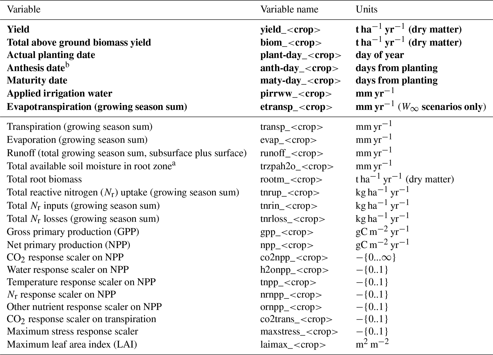
Table 2Output variables, naming convention, and units in the GGCMI Phase 2 protocol. Items in bold text are the mandatory minimum requirements (if model capacities allow for these outputs). Other variables are optionally provided depending on availability and participating modeling groups provided between 3 (PEPIC) and 18 (APSIM-UGOE) of these optional variables.
a Growing season sum, basis for computing average soil moisture. b Provided where possible.
All models in GGCMI Phase 2 provide 30-year time series of annual crop yields for each scenario, 0.5∘ grid cell and crop, in units of t ha−1 yr−1. They also provide all available variables of the following six: total aboveground biomass yield; the dates of planting, anthesis and maturity; applied irrigation water in irrigated scenarios; and total evapotranspiration. We term these seven variables the “mandatory” outputs, but note that some models do not compute all of them; e.g., CARAIB does not compute the anthesis date. Besides these seven “mandatory” data products (Table 2, bold), the protocol requests any or all of 18 “optional” additional output variables (Table 2, plain text). Participating modeling groups provided between 3 (PEPIC) and 18 (APSIM-UGOE) of these optional variables.
All output data are supplied as NetCDF version 4 files, each containing values for one variable in a 30-year time series associated with a single scenario, for all grid cells. Filenames follow the naming conventions of GGCMI Phase 1 (Elliott et al., 2015), which themselves are derived from those of ISIMIP (Frieler et al., 2017). Filenames are specified as [model]_[climate]_hist_fullharm_[variable]_[crop] _global_annual_[start-year]_[end-year]_[C]]_[T]_[W]_[N]_[A].nc4 Here, [model] is the crop model name; [climate] is the original climate input dataset (typically AgMERRA); [variable] is the output variable (of those in Table 2); [crop] is the crop abbreviation (“mai” for maize, “ric” for rice, “soy” for soybean, “swh” for spring wheat, and “wwh” for winter wheat); and [start-year] and [end-year] specify the first and last years recorded on file. [C], [T], [W], [N], and [A] indicate the CTWN-A settings, each represented with the respective uppercase letter and the number indicating the level (e.g., “C360_T0_W0_N200”; see Table 1). Except for the CTWN-A letters, the entire filename needs to be in small caps. All filenames include the identifiers global and annual to distinguish them as global, annual model output, following the updated ISIMIP file naming convention (Frieler et al., 2017).
Output data are provided on a regular geographic grid, identical for all models. Grid cell centers span latitudes from −89.75 to 89.75∘ and longitudes from −179.75 to 179.75∘. Missing values where no crop growth has been simulated are distinguished from crop failures: a crop failure is reported as zero yield but non-simulated areas (including ocean grid cells) have yields reported as “missing values” (defined as 1×10²⁰ in the NetCDF files). Following NetCDF standards, latitude, longitude, and time are included as separate variables in ascending order, with units “degrees north”, “degrees east”, and “growing seasons since 1 January 1980 00:00:00”.
Following GGCMI Phase 1 standards, the first entry in each file describes the first complete cropping cycle simulated from the given climate input time series. In the AgMERRA time series used for GGCMI Phase 2, the first year provided is 1980 but the date of the first entry can vary by crop and location. In the Northern Hemisphere, for summer crops like maize (sown in spring 1980 and harvested in fall 1980), the first harvest record would be of 1980, but for winter wheat (sown in fall 1980 and harvested in spring 1981) the first harvest record would be of 1981. Output files report the sequence of growing periods rather than calendar years. While there is generally one sowing event per calendar year (since simulations with harmonized growing seasons do not permit double cropping), in some cases harvest events may skip or repeat within a calendar year. For example, because soybeans in North Carolina are typically harvested well into December, some calendar years may include no harvest (if it is not completed until after 31 December) or two harvests (one in January and one 11 months later in the following December).
The 12 models participating in GGCMI Phase 2 are listed in Table 3. Models differ substantially in structure and parameterization and can be separated into two broad categories: site-based (field-scale) models and global ecosystem models. The six site-based models are APSIM, pDSSAT, and the EPIC family of models; the six ecosystem models are LPJmL, LPJ-GUESS, PROMET, CARAIB, Organising Carbon and Hydrology In Dynamic Ecosystems (ORCHIDEE), and JULES. Models employ a variety of approaches for the core modules such as primary production or evapotranspiration. For primary production, site-based models employ light use efficiency approaches and ecosystem models use photosynthesis approaches. For evapotranspiration, most models use Priestley–Taylor, Penman–Monteith or Hargreaves schemes, but JULES and PROMET utilize a land surface model approach instead. Note that models that share a common genealogy may still use different schemes for evapotranspiration: for example, EPIC-TAMU uses Penman–Monteith and EPIC-IIASA uses Hargreaves. To describe soils, most models use either the Harmonized World Soil Database (HWSD) from the FAO (FAO/IIASA/ISRIC/ISSCAS/JRC, 2012) or the ISRIC-WISE database (Batjes, 2005) or a derivation thereof. Table S1 in the Supplement provides details on these model characteristics as well as on implementation, including spin-up, calibration other than growing season, residue management, and irrigation rules.
Keating et al. (2003)Holzworth et al. (2014)Dury et al. (2011)Pirttioja et al. (2015)Balkovič et al. (2014)Izaurralde et al. (2006)Osborne et al. (2015)Williams and Falloon (2015)Williams et al. (2017)Liu et al. (2007)Folberth et al. (2012)Lindeskog et al. (2013)Olin et al. (2015)von Bloh et al. (2018)Wu et al. (2016)Elliott et al. (2014b)Jones et al. (2003)Liu et al. (2016a)Liu et al. (2016b)Hank et al. (2015)Mauser et al. (2015)Zabel et al. (2019)Table 3Models included in GGCMI Phase 2 and the number of CTWN-A simulations performed. The maximum number is 756 for A0 (no adaptation) experiments, and 648 for A1 (maintaining growing length) experiments, since T0 is not simulated under A1. “N dim” indicates whether the models are able to represent varying nitrogen levels. Each model provides the same set of CTWN simulations across all its modeled crops, but some models omit individual crops. (For example, APSIM-UGOE does not simulate winter wheat.) Bold numbers indicate those models that provided all specified simulations (with or without varying nitrogen).
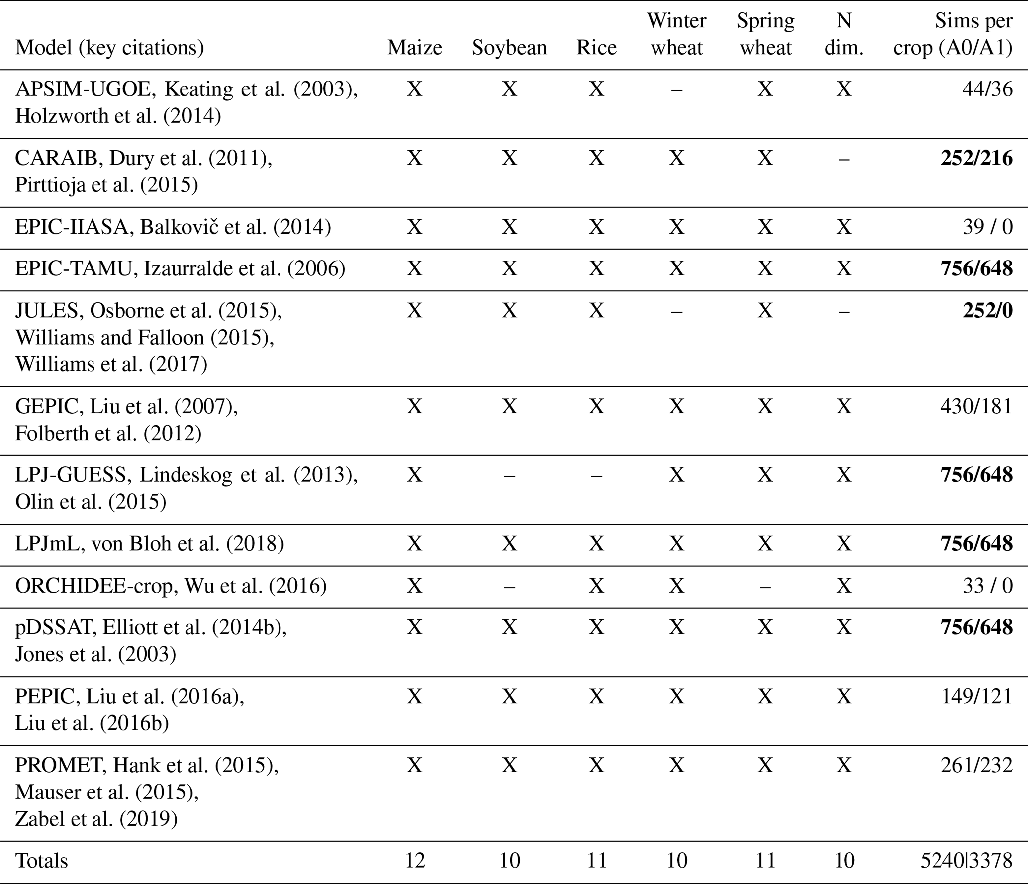
Table 3 also describes the simulation output contribution of each model to the GGCMI Phase 2 archive. Not all modeling groups provided simulations for the full protocol described above. Given the substantial computational requirements, different participation tiers were specified to allow submission of smaller subsets of the full protocol. These subsets were designed as alternate samples across the four dimensions of the CTWN space, with full (12) and low (4) options for the C⋅N variables, and full (63), reduced (31), and minimum (9) options for T⋅W variables (described below). All participating modeling groups provided identical coverage of the CTWN parameter space for different crops, but most differed in CTWN coverage of A0 and A1 scenarios. Since the adaptation dimension was defined as a secondary priority for GGCMI Phase 2, some models provided a more limited set of A1 scenarios. Of these, EPIC-IIASA, JULES, and ORCHIDEE-crop provided no A1 scenarios.
The different participation levels are defined by combining the C⋅N sets with the T⋅W sets:
-
full: all 756 A0 simulations (all 12 C×N* all 63 T×W);
-
high: 362 simulations (all 12 C×N combinations ⋅ reduced T×W set of 31 combinations);
-
mid: 124 simulations (low 4 C×N combinations ⋅ reduced T×W set of 31 combinations); and
-
low: 36 simulations (low 4 C×N combinations ⋅ minimum T×W set of 9 combinations).
Of the 12 models submitting data, six followed the full protocol; these are marked with bold text in the last column of Table 3. However, note that two of these models (CARAIB and JULES) cannot represent nitrogen effects explicitly and so do not sample over the nitrogen dimension. Two models followed high with minor modifications (GEPIC adding an additional T level and PROMET omitting the intermediate N level). One model (PEPIC) followed mid but included an additional C level. Three models approximately followed low with APSIM-UGOE and EPIC-IIASA providing some additional T×W levels and ORCHIDEE-crop omitting some T×W combinations.
The combinations of perturbation values in the C×N and T×W parameter spaces used in the various participation levels are chosen to provide maximum coverage over plausible future values. For the C×N space, we specify
-
full as 12 pairs, with four C values (360, 510, 660, 810 ppm) and three N values (10, 60, 200 kg ha−1 yr−1) and
-
low as only four pairs: C360_N10, C360_N200, C660_N60, and C810_N200.
For the T×W space, we specify
-
full as all seven T levels and nine W levels;
-
reduced as 31 alternating combinations, with different Ws for even Ts than for odd Ts. For even Ts (i.e., T0, T2, T4, T6), we use , −20, 0, pairs. For odd Ts (i.e., T−1, T1, T3), we use , −10, +10, +30, inf = pairs;
-
minimum as nine combinations: , T0W10, T1W−30, T2W−50, T2W20, T3W30, T4W0, T4Winf, T6W−20.
To illustrate the properties of the GGCMI Phase 2 model simulations, we provide an evaluation of model performance by comparing model and historical yields, and show example results that demonstrate the spread of model responses to climate and management inputs.
4.1 Evaluation of model performance
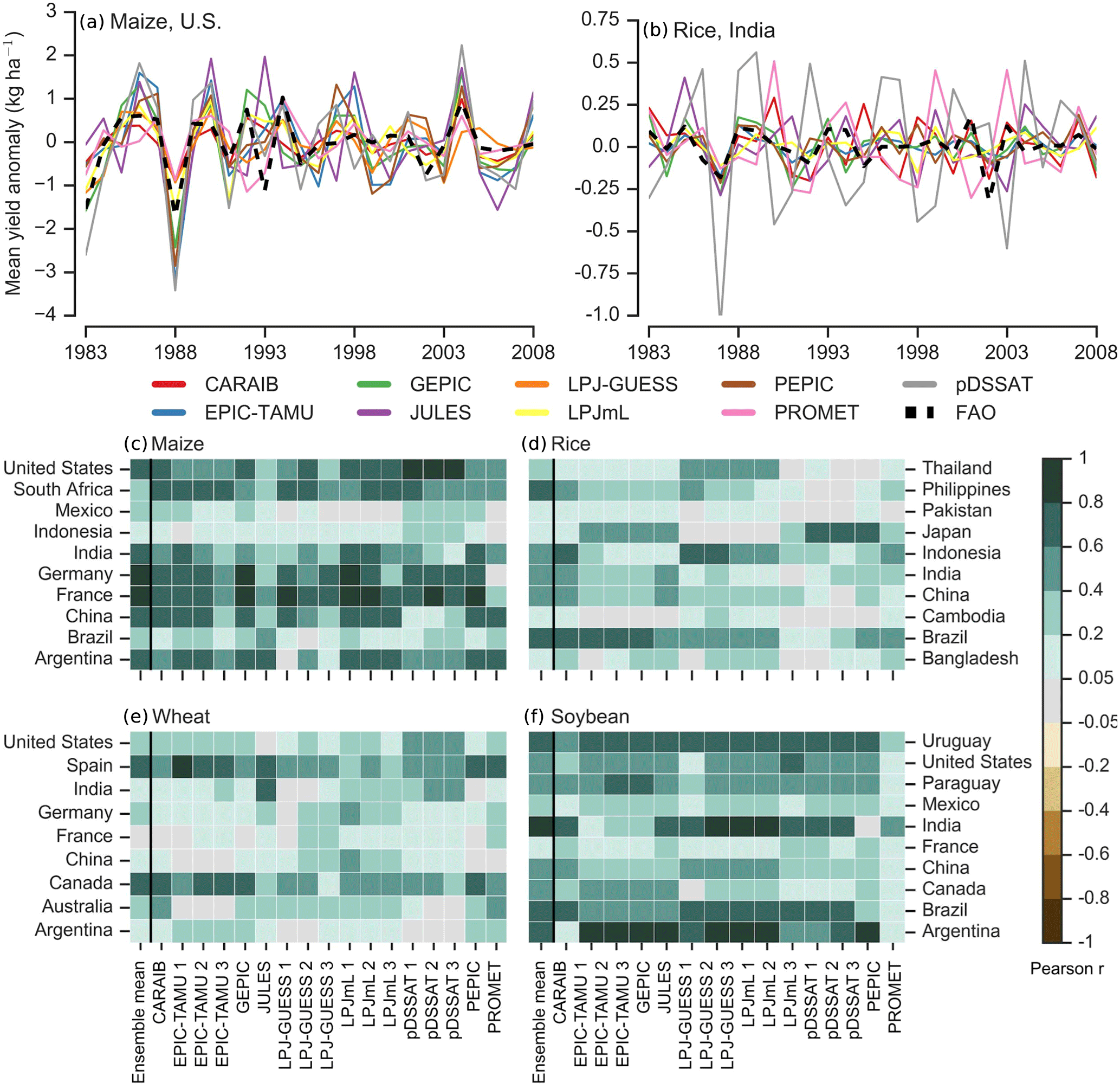
Figure 2Assessment of crop model performance in GGCMI Phase 2, following the protocol of GGCMI Phase 1 (Müller et al., 2017). (a, b) Example time series comparison between simulated crop yield and FAO country statistics (FAO, 2018) at the country level for two example high production countries: US maize and rice in India, both for the 200 kg ha−1 nitrogen application level. (c–f) Heatmaps illustrating the Pearson r correlation coefficient between the detrended simulated and observed country-level mean yields for the top 10 countries by production for each crop, of those countries with continuous FAO data over 1981–2010. We show separate comparisons for simulations with the three different nitrogen application levels, denoted 1, 2, and 3 for 10, 60, and 200 kg N ha−1, respectively. Panels (a, c, e) show correlation of ensemble mean yields with FAO data. Because FAO does not distinguish between wheat types, we sum simulated spring and winter wheat for models that provide both (see Table 3). Note that differences by region and crop are stronger than difference between models; e.g., horizontal bars are more similar in color than vertical bars. Countries are ordered alphabetically, not by production quantity.
All models participating in GGCMI Phase 2 have be evaluated against historical yields and site-specific experimental data. Most models (9 of 12, all but CARAIB, JULES, and PROMET) have been evaluated in their global setup in the GGCMI Phase 1 evaluation exercise (Müller et al., 2017), and many have used the GGCMI Phase 1 online tool to similarly evaluate subsequent model versions (e.g., von Bloh et al., 2018). Evaluating the performance of crop models in the GGCMI Phase 2 archive is complicated by the artificial nature of the protocol: the settings in the CTWN-A experiment design do not reflect actual conditions in the real world. The protocol includes one scenario of near-historical climate inputs (T0, W0, C360), but the prescribed uniform nitrogen application levels do not reflect real-world fertilizer practices. Models also omit detailed calibrations to reflect the performance of historical cultivars.
We provide a partial evaluation of the models' skill in reproducing crop yield characteristics using the methodology of Müller et al. (2017), developed for GGCMI Phase 1. Müller et al. (2017) evaluate how well model crop yield responses in a historical run capture real-world yield variations driven by year-to-year temperature and precipitation variations. Following this approach, we compare yields in the GGCMI Phase 2 baseline simulations with detrended historical yields from the Food and Agriculture Organization of the United Nations (FAO, 2018) by calculating the Pearson product moment correlation coefficient over 26 years of yield. The procedure is sensitive to the detrending method and the area mask used to aggregate yields; we use a 5-year running mean removal and the MIRCA2000 cultivation area mask for aggregation. In some cases, the model time series are shifted by 1 year to account for discrepancies in FAO or model year reporting. Because the GGCMI Phase 2 protocol imposes fixed, uniform nitrogen application levels that are not realistic for individual countries, we evaluate control runs for each model at multiple N levels whenever possible. Overall, nine of the GGCMI Phase 2 models (Table 3) provide historical runs for all three nitrogen levels (10, 60, and 200 kg ha−1 yr−1).
As expected due to the unrealistic features described above, correlation coefficients for the GGCMI Phase 2 simulations are slightly lower than those found in the Phase 1 evaluation, but models show reasonable fidelity at capturing year-to-year variation (Fig. 2). For example, global correlation coefficients in Phase 1 and Phase 2, respectively, are 0.89 and 0.74 for maize, 0.67 and 0.64 for wheat, and 0.64 and 0.59 for soybeans. (Phase 1 values are from Figs. 1–4 and 6 in Müller et al., 2017.) Differences in fidelity between regions and crops exceed differences between models; that is, Fig. 2c–f show more color similarity in horizontal than vertical bars. For example, maize in the United States is consistently well simulated, while maize in Indonesia is problematic (mean Pearson correlation coefficients of 0.68 and 0.18, respectively). Note that in this methodology, simulations of crops with low year-to-year variability such as irrigated rice and wheat will tend to score more poorly than those with higher variability. In some cases, especially in the developing world, low correlation coefficients may point to reporting problems in the FAO statistics and to real-world variability caused by variations in management rather than weather (Ray et al., 2012; Müller et al., 2017). No single model consistently exhibits greater fidelity than others. Instead, each model shows near best-in-class performance for at least one location–crop combination. For example, pDSSAT is the best model for maize in the US, LPJmL and GEPIC are best in Germany, PROMET is best in Argentina, and PEPIC and LPJ-GUESS are best in France.
4.2 Model crop yield responses under CTWN forcing
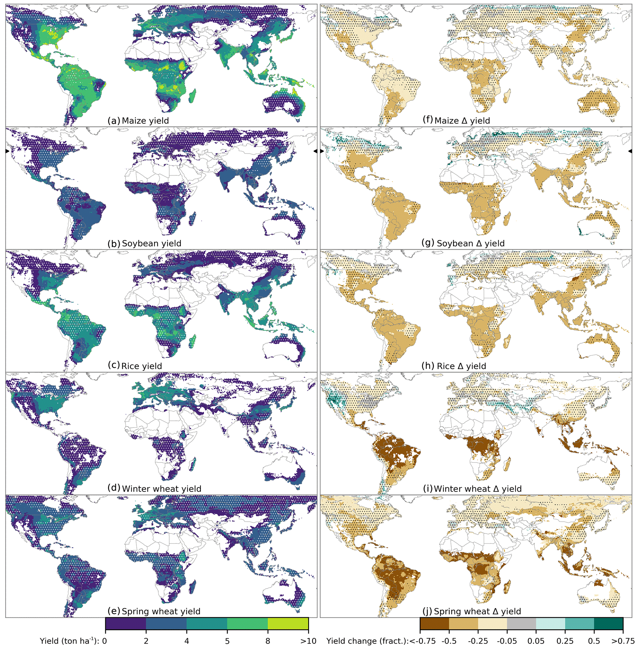
Figure 3Illustration of the spatial patterns of baseline yields (a–e) and yield changes (f–j) in the GGCMI Phase 2 ensemble. The left column shows multi-model climatological (30-year) median yields for the baseline scenario, with white stippling indicating areas where these crops are not currently cultivated. Areas with less than 0.5 t ha−1 in the baseline are masked. Absence of cultivation aligns well with the lowest yield contour (0–2 t ha−1). The right column shows multi-model mean fractional yield changes in the T+4 ∘C scenario relative to the baseline scenario. Areas without stippling are those where models agree on changes: the multi-model mean fractional change exceeds the standard deviation of changes in individual models. Stippling indicates areas of low confidence (Δ<1σ). Some spatial structure in projected changes at high latitudes may be due to differences in model coverage; see Fig. 1.
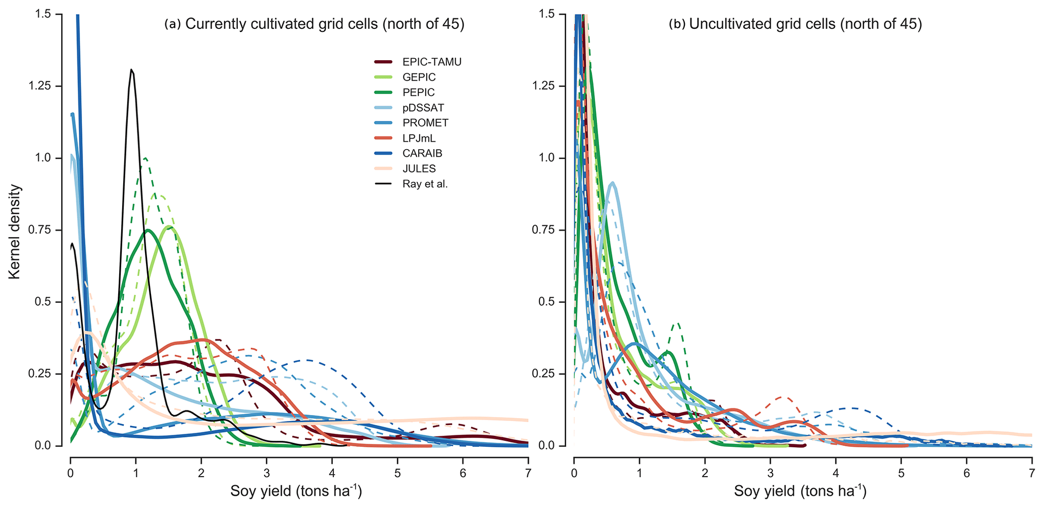
Figure 4Model probability densities for soybean yields at latitudes north of 45∘ in historical and warming simulations in the A0 case. While 10 GGCMI Phase 2 models provide simulations (Table 3); we show eight representative models for clarity. Probability density functions are estimated separately for locations with some current cultivation (a, approximately 2500 grid cells, unweighted by cultivated area) and for uncultivated locations (b, approximately 1500 grid cells), for baseline historical (solid) and T+4 (∘C) (dashed) simulations. Black line in panel (a) shows actual yields from 1997 to 2003 derived from Ray et al. (2012). For historical simulations, models agree on low potential yields in currently uncultivated areas (b) but disagree widely on yields in currently cultivated areas (a). Color code groups models into those with realistic yield distributions peaking at 1–2 t ha−1 (green), those with flatter distributions extending to unrealistically high values (red), and those with predominantly zero yields (blue). “Green” models show slight decreases under T+4 warming, “red” models moderate increases, and “blue” models large increases.
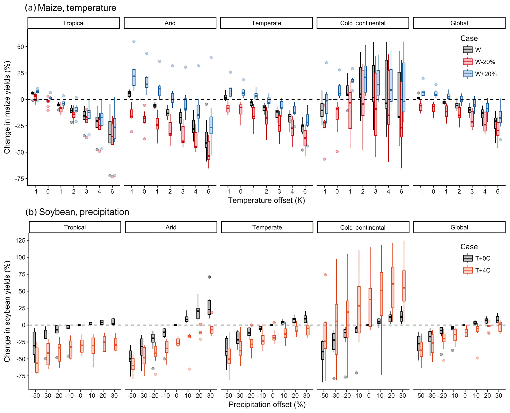
Figure 5Illustration of the distribution of regional yield changes across the multi-model ensemble, split by Köppen–Geiger climate regions, and with global response in rightmost panel. The y axis is the fractional change in the regional average climatological (30-year mean) potential yield relative to the baseline. Box-and-whisker plots show distribution across models, with median marked; edges are first and third quartiles and whiskers extend to 1.5⋅IQR. The figure shows all simulated grid cells for each model; see Figs. S10–S13 for only currently cultivated land. We highlight responses to individual factors; note that results are not directly comparable to simulations of realistic projected climate scenarios with identical global mean changes. Models generally agree outside high-latitude regions, with projected changes exceeding inter-model variance. (a) Response of rainfed maize to applied uniform temperature perturbations, for three discrete precipitation perturbation levels (−20 %, 0 %, and +20 %), with CO2 and nitrogen held constant at baseline values (360 pmm and 200 kg ha−1 yr−1). Outliers in the tropics (strong negative impact of higher T) are the pDSSAT model; outliers in the arid region (strong positive impact of higher P) are JULES. (b) Response of rainfed soybeans to applied uniform precipitation perturbations, for two discrete temperature levels. Cases with reduced precipitation show greater inter-model spread than those with increased precipitation. At very large precipitation increases, yield changes level out: benefits saturate once water availability is no longer limiting. Precipitation changes are more important in the arid region, as expected. Note the large uncertainty in the cold continental region, also illustrated in Figs. 3 and 4.
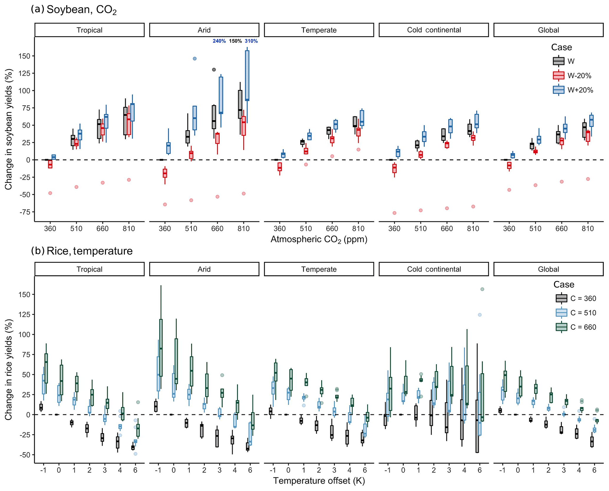
Figure 6Illustration of the distribution of regional yield changes across the multi-model ensemble, here for soybeans and rice for the A0 case. Conventions are as in Fig. 5. (a) Response of rainfed soybeans to atmospheric CO2, for three discrete precipitation perturbation levels with temperature and nitrogen held constant at baseline values. Low outliers are the EPIC-TAMU model and the high outliers in the arid region are the JULES model. Reduced precipitation tends to steepen the CO2 response and increased precipitation tends to flatten it, as expected. Reduced precipitation tends to increase the inter model spread, especially at the highest CO2 levels. (b) Response of irrigated rice for three discrete CO2 levels, with nitrogen and precipitation held constant. CO2 does not change the nature of temperature response respective to baseline as the slopes at each CO2 level are relatively constant.
Crop models in the GGCMI Phase 2 ensemble show broadly consistent responses to climate and management perturbations in most regions, with a strong negative impact of increased temperature in all but the coldest regions. Mapping the distribution of baseline yields and yield changes shows the geographic dependencies that underlie these results. Absolute yield potentials show strong spatial variation, with much of the Earth's surface area unsuitable for any of these crops (Fig. 3, left). Crop yield changes under climate perturbations also show distinct geographic patterns (Fig. 3, right, which shows fractional yield differences between the baseline and T+4 A0 scenarios). In general, models agree most on yield response in regions where yield potentials are currently high and therefore where crops are currently grown. In A0 simulations, models show robust decreases in yields at low latitudes, and highly uncertain ensemble mean increases at most high latitudes. Low-latitude yield reductions are due in part to shortening of the growing season under warming and in part to the direct effects of higher temperature. In A1 simulations, where growing seasons length does not change, temperature-related reductions in yield are more muted (see Fig. S14). In both A0 and A1 simulations, models show some increases in high mountain regions that are currently cold limited.
Projections of strong yield growth at higher latitudes should be treated with caution, since the effects evident in Fig. 3 are due in part to inaccuracies in model representations of present-day crop yields. For example, at latitudes north of 45∘, the GGCMI Phase 2 models collectively suggest strong (but uncertain) growth in soybean yields under warmer conditions (Fig. 3g). However, model differences are greater in the baseline than future simulations and greatest in currently cultivated areas (Fig. 4). Both the mean projected growth and the inter-model spread are driven by three models that show almost zero present-day potential soybean yields across the entire high-latitude region, even in locations where soybeans are currently grown (Fig. 4, left). PROMET, for example, involves a stronger response to cold than other models (e.g., LPJmL) with frost below −8 ∘C irreversibly killing non-winter crops and prolonged periods of below-optimum temperatures also leading to complete crop failure. Over the high-latitude regions simulated by both models, 52 % of grid cells in PROMET report 0 yield in the present climate vs. 11 % of cells in the T+4 scenario, leading to a strong yield gain in warmer future climates. In LPJmL outputs, the same high-latitude area is deemed suitable for cultivation even in baseline climate, with crop failure rates of 4 % and 5 % in present and T+4 cases, so that projected yield changes are modest (Fig. 4). These spurious low baseline yields result in very large fractional changes in the T+4 warming scenario, when all models agree that conditions become favorable for soybeans. Those models that most accurately reproduce present-day high-latitude soybean yields of 1–2 t ha−1 (Ray et al., 2012) in fact show a slight decrease in yield under a warming scenario (Fig. 4a). Apparent future yield increases in the multi-model mean are driven by the least realistic simulations.
The GGCMI Phase 2 exercise offers the opportunity to examine and characterize not just crop response to a single temperature change but nonlinearities in responses and interactions between factors. We illustrate a few of these relationships in Figs. 5–6 using A0 simulations to capture maximum climate effects. We choose crops and factors whose effects are reasonably well understood and show that these are reproduced in models. It is expected, for instance, that increases in precipitation should buffer the effects of warmer temperatures and that CO2 increases should reduce damage to crops in scenarios where water is limited. Models generally confirm expected behavior but also provide insight into unforeseen interactions. To show geographic effects, we divide model responses in Figs. 5–6 by the primary Köppen–Geiger climate regions (Rubel and Kottek, 2010), showing the yield changes across all simulated grid cells in each region. In each panel, we examine relationships between two factors, showing yield response against one for several scenarios of the other, in box plots that show the inter-model spread. The responses highlighted here are qualitatively similar across all crops included in this study (Figs. S5–S9 for all simulated area and S10–S13 for cultivated area only).
For all crops, warming scenarios with precipitation held constant produce yield decreases in most regions. These impacts are robust for even moderate climate perturbations. For rainfed maize, even a 1 ∘C temperature increase with other factors held constant produces a median regional decline in potential yield that exceeds the variance across models, in all but the “cold-continental” regions (Fig. 5a). The remaining areas (“warm temperate”, “equatorial”, and “arid”) account for nearly three-quarters of global maize production. In the high-latitude “cold-continental” region, potential yield changes are positive but highly uncertain, for the reasons discussed previously; uncertainties are larger even for maize than for soybeans. (Compare Fig. 5a and b.) Temperature effects are somewhat nonlinear, with the largest impacts for maize in the warm “tropical” region (for soybeans, temperature effects are more complex; see Fig. S5). Precipitation effects on rainfed crops are more strongly nonlinear. The curvature of the precipitation response can be seen by eye in Fig. 5b: soybean yields are strongly negatively impacted by reduced rainfall, peak under increased precipitation of 20 %, and actually decline at higher precipitation levels.
As expected, precipitation and temperature effects interact, with increases in precipitation buffering yield responses to temperature. Increased rainfall mitigates the negative impacts of warmer temperatures caused by increased evapotranspiration (e.g., Allen et al., 1998). For maize, the effect is relatively modest outside the “arid” regions (Fig. 5a). Globally, a 4 ∘C temperature rise with no change in precipitation results in median loss of ∼13 % of rainfed maize, with all models showing a negative response. With a 20 % increase in precipitation, the median yield loss is ∼8 %. For soybeans, the equivalent values are ∼11 % and 1 %, respectively. Decreased rainfall, on the other hand, amplifies yield losses and also increases inter-model variance. That is, models agree that the response to decreased water availability is negative in sign but disagree on its magnitude. Outside of arid regions, the interaction effect itself shows little nonlinearity (i.e., response slopes in Fig. 5a and b are roughly parallel). As expected, irrigated crops are more resilient to temperature increases in all regions, especially so where water is already limiting (other than winter wheat; Fig. S9).
Increased CO2 boosts yields overall through the well-known CO2 fertilization effect (Fig. 6). The effect is strongest for the C3 crops (wheat, soybeans, and rice), while maize, a C4 grass, has a comparatively muted response. We show irrigated rice and rainfed soy in Fig. 6 as representative C3 crops. The effect of CO2 on yields is nonlinear, as expected, with significant benefit from small increases but with effects plateauing at higher concentrations (Fig. 6). CO2 and temperature effects show minimal interaction. This effect is seen in Fig. 6a, which shows nearly parallel response slopes at different CO2 levels. That is, CO2 fertilization does little to change the nature of the temperature response. On the other hand, CO2 and precipitation effects interact strongly, as expected since higher CO2 levels allow reduced stomatal conductance and evapotranspiration losses, mitigating the effect of reduced rainfall (e.g., McGrath and Lobell, 2013). This interaction is seen in Fig. 6b as smaller yield losses from reduced rainfall when CO2 levels are higher. For example, for soy, raising CO2 to 510 ppm actually outweighs the multi-model median damages caused by a 20 % precipitation reduction in all climate regions. All crops show similar behavior, but note that model uncertainties for wheat are substantially higher than those for other crops. (Compare Fig. 6a for soy and Fig. S7 for wheat.)
We show some additional cases in the Supplement. As noted previously, the A1 adaptation simulations involve significantly moderated temperature impacts relative to the A0 simulations shown here (Fig. S14). Figures S15 and S16 show the response in the nitrogen dimension and an irrigation water demand response example.
The GGCMI Phase 2 experiment provides a database designed to allow detailed study of crop yields in process-based models under climate change. While previous crop model intercomparison projects in the climate change context have focused on simulations along realistic projected climate scenarios (e.g., Rosenzweig et al., 2014), the use of systematic input parameter variations in GGCMI Phase 2, with up to 756 scenarios, allows not only comparing yield sensitivities to changing climate and management inputs but also evaluating the complex interactions between important driving factors: CO2, temperature, water supply, and applied nitrogen. The global extent of the experiment also allows identifying geographic shifts in high potential yield locations. With 12 participating models and 31 simulation years per scenario, the complete database constitutes over 150 000 years of gridded global yield simulation output for each crop.
Preliminary results shown here highlight some of the insights facilitated by the simulation exercise and lend confidence in the models. In validation tests of historical simulations, year-to-year correlations in modeled and actual country-level yields are similar to those of GGCMI Phase 1. In simulations of scenarios with perturbed climate and management factors, models broadly agree on changes outside the high latitudes, with the magnitude of changes at nearly all perturbation levels exceeding the inter-model spread. At high latitudes, differences between models may result from differences in their assumed yields in current cold conditions. In simulations with multiple perturbations, interactions between major yield drivers (e.g., temperature and precipitation in Fig. 5, or precipitation and CO2 in Fig. 6) generally follow expectations and produce physically reasonable responses in crop yields.
Users should however be aware of some limitations of the GGCMI Phase 2 experiment that affect its potential applications. First, absolute yield values in the baseline scenario, driven by 1981–2010 historical climate, will generally not match observed yields over this time period. In order to match current yields, process-based models must be re-tuned to account for the constant evolution of crop cultivar genetics and management practice (e.g., Jones et al., 2017). GGCMI Phase 2 is intended as a study of model responses to changes in climatic conditions, which are assumed insensitive to the adjustments needed to reproduce present-day yields. The baseline scenario also includes no trend in CO2, and no individual case involves realistic country-specific nitrogen application levels (Elliott et al., 2015).
The second major caveat is that no individual GGCMI Phase 2 simulation is itself a realistic future yield projection. The uniform applied offsets in temperature and precipitation sample over potential changes, and do not individually capture the spatially heterogeneous warming and precipitation changes expected in realistic climate projections. GGCMI Phase 2 simulation results can be used for impacts projection but only with the construction of an emulator of crop yield response to climatological changes, which can then be driven by arbitrary climate scenarios. Such emulators are shown to accurately reproduce crop model output under realistic climate projections, even though the GGCMI Phase 2 experiment does not sample over potential changes in the higher-order moments in temperature and precipitation distributions (Franke et al., 2020). Note that some factors that may affect future climate-driven yield impacts cannot be captured by the GGCMI Phase 2 models in any usage, since models do not include representations of pests, diseases, and weeds. Offline crop model simulations (i.e., with prescribed rather than dynamically simulated atmospheric conditions) can also not capture any feedbacks on the climate from land use, such as irrigation impacts on humidity (e.g., Decker et al., 2017).
We expect that the GGCMI Phase 2 simulations will yield multiple insights in future studies. Potential applications include, as mentioned, the construction of emulators and yield response surfaces that can be used for both model diagnosis and impacts assessment. Specific studies could include analyzing the drivers of temperature-related yield losses (which may be due to both direct thermal effects or to shortening growing seasons); the benefits of adaptation; interactions between CO2 and water or other CTWN factors affecting yield; changes in nitrogen use efficiency; geographic shifts in regional production; and regional differences in yield sensitivities to CTWN-A factors. Emulators based on the dataset can be used to identify hotspots of crop system vulnerability and to conduct rapid assessment of new climate projections. In general, the development of multi-model ensembles involving systematic parameter sweeps has large promise both for increasing understanding of potential future crop responses and for improving process-based crop models.
Table 4DOIs for model data outputs. All model output data can be found at https://doi.org/10.5281/zenodo/XX, where XX is the value listed in the table.
All input data are available via zenodo at https://doi.org/10.5281/zenodo.3773827 (Müller et al., 2020). For the minimum cropland mask, choose the boolean_cropmask_ggcmi_phase2.nc4 file. Growing period data for wheat are now divided up into winter and spring wheat, whereas all other growing season data (maize, rice, soybean) are the same as in Phase 1.
The supplement related to this article is available online at: https://doi.org/10.5194/gmd-13-2315-2020-supplement.
JE, CM, and ACR designed the research. CM, JJ, JB, PC, MD, PF, CF, LF, MH, RCI, IJ, CJ, NK, MK, WL, SO, MP, TAMP, AR, XW, KW, and FZ performed the simulations. JF, JJ, CM, and EM performed the analysis, and JF, EM, and CM prepared the manuscript. All authors contributed to editing the manuscript.
The authors declare that they have no conflict of interest.
This research was performed as part of the Center for Robust Decision-making on Climate and Energy Policy (RDCEP) at the University of Chicago. This is paper number 35 of the Birmingham Institute of Forest Research. Computing resources were provided by the University of Chicago Research Computing Center (RCC). We thank two anonymous reviewers for their helpful comments.
RDCEP is funded by NSF (grant no. SES-1463644) through the Decision Making Under Uncertainty program. James Franke was supported by the NSF NRT program (grant no. DGE-1735359) and the NSF Graduate Research Fellowship Program (grant no. DGE-1746045). Christoph Müller was supported by the MACMIT project (grant no. 01LN1317A) funded through the German Federal Ministry of Education and Research (BMBF). Alex C. Ruane was supported by NASA NNX16AK38G (INCA) and the NASA Earth Sciences Directorate/GISS Climate Impacts Group. Christian Folberth was supported by the European Research Council Synergy (grant no. ERC-2013-SynG-610028) Imbalance-P. Pete Falloon and Karina Williams were supported by the Newton Fund through the Met Office program Climate Science for Service Partnership Brazil (CSSP Brazil). Karina Williams was supported by the IMPREX research project supported by the European Commission under the Horizon 2020 Framework program (grant no. 641811). Stefan Olin acknowledges support from the Swedish strong research areas BECC and MERGE, together with support from LUCCI (Lund University Centre for studies of Carbon Cycle and Climate Interactions). R. Cesar Izaurralde acknowledges support from the Texas Agrilife Research and Extension, Texas A & M University.
This paper was edited by David Lawrence and reviewed by two anonymous referees.
Allen, R., Pereira, L., Dirk, R., and Smith, M.: Crop evapotranspiration-Guidelines for computing crop water requirements, FAO Irrigation and drainage paper 56, 1998. a
Angulo, C., Rötter, R., Lock, R., Enders, A., Fronzek, S., and Ewert, F.: Implication of crop model calibration strategies for assessing regional impacts of climate change in Europe, Agr. For. Meteorol., 170, 32–36, https://doi.org/10.1016/j.agrformet.2012.11.017, 2013. a
Asseng, S., Ewert, F., Rosenzweig, C., Jones, J., Hatfield, J., Ruane, A., J. Boote, K., Thorburn, P., Rötter, R. P., Cammarano, D., Brisson, N., Basso, B., Martre, P., Aggarwal, P., Angulo, C., Bertuzzi, P., Biernath, C., Challinor, A., Doltra, J., Gayler, S., Goldberg, R., Grant, R., Heng, L., Hooker, J., Hunt, L. A., Ingwersen, J., Izaurralde, R. C., Kersebaum, K. C., Müller, C., Kumar, S. N., Nendel, C., Leary, G. O., Olesen, J. E., Osborne, T. M., Palosuo, T., Priesack, E., Ripoche, D., Semenov, M. A., Shcherbak, I., Steduto, P., Stöckle, C., Stratonovitch, P., Streck, T., Supit, I., Tao, F., Travasso, M., Waha, K., Wallach, D., Williams, J. R., and Wolf, J.: Uncertainty in simulating wheat yields under climate change, Nat. Clim. Change, 3, 827–832, https://doi.org/10.1038/nclimate1916, 2013. a
Asseng, S., Ewert, F., Martre, P., Rötter, R. P., B. Lobell, D., Cammarano, D., A. Kimball, B., Ottman, M., W. Wall, G., White, J., Reynolds, M., D. Alderman, P., Prasad, P. V. V., Aggarwal, P., Anothai, J., Basso, B., Biernath, C., Challinor, A., De Sanctis, G., Doltra, J., Fereres, E., Garcia-Vila, M., Gayler, S., Hoogenboom, G., Hunt, L. A., Izaurralde, R. C., Jabloun, M., Jones, C. D., Kersebaum, K. C., Koehler, A.-K., Muller, C., Naresh Kumar, S., Nendel, C., O/'Leary, G., Olesen, J. E., Palosuo, T., Priesack, E., Eyshi Rezaei, E., Ruane, A. C., Semenov, M. A., Shcherbak, I., Stockle, C., Stratonovitch, P., Streck, T., Supit, I., Tao, F., Thorburn, P. J., Waha, K., Wang, E., Wallach, D., Wolf, J., Zhao, Z., and Zhu, Y.: Rising temperatures reduce global wheat production, Nat. Clim. Change, 5, 143–147, https://doi.org/10.1038/nclimate2470, 2015. a
Balkovič, J., van der Velde, M., Skalský, R., Xiong, W., Folberth, C., Khabarov, N., Smirnov, A., Mueller, N. D., and Obersteiner, M.: Global wheat production potentials and management flexibility under the representative concentration pathways, Global Planet. Change, 122, 107–121, https://doi.org/10.1016/j.gloplacha.2014.08.010, 2014. a
Batjes, N.: ISRIC-WISE global data set of derived soil properties on a 0.5 by 0.5 degree grid (Ver. 3.0), 2005. a
Bodirsky, B. L., Rolinski, S., Biewald, A., Weindl, I., Popp, A., and Lotze-Campen, H.: Global Food Demand Scenarios for the 21st Century, PLOS ONE, 10, 1–27, https://doi.org/10.1371/journal.pone.0139201, 2015. a
Boote, K., Jones, J., White, J., Asseng, S., and Lizaso, J.: Putting Mechanisms into Crop Production Models, Plant Cell Environ., 36, 1658–1672, https://doi.org/10.1111/pce.12119, 2013. a
Challinor, A. J., Müller, C., Asseng, S., Deva, C., Nicklin, K. J., Wallach, D., Vanuytrecht, E., Whitfield, S., Ramirez-Villegas, J., and Koehler, A.-K.: Improving the use of crop models for risk assessment and climate change adaptation, Agr. Syst., 159, 296–306, 2018. a, b
Decker, M., Ma, S., and Pitman, A.: Local land–atmosphere feedbacks limit irrigation demand, Environ. Res. Lett., 12, 054003, https://doi.org/10.1088/1748-9326/aa65a6, 2017. a
Dee, D. P., Uppala, S. M., Simmons, A. J., Berrisford, P., Poli, P., Kobayashi, S., Andrae, U., Balmaseda, M. A., Balsamo, G., Bauer, P., Bechtold, P., Beljaars, A. C. M., van de Berg, L., Bidlot, J., Bormann, N., Delsol, C., Dragani, R., Fuentes, M., Geer, A. J., Haimberger, L., Healy, S. B., Hersbach, H., Hólm, E. V., Isaksen, L., Kållberg, P., Köhler, M., Matricardi, M., McNally, A. P., Monge-Sanz, B. M., Morcrette, J.-J., Park, B.-K., Peubey, C., de Rosnay, P., Tavolato, C., Thépaut, J.-N., and Vitart, F.: The ERA-Interim reanalysis: configuration and performance of the data assimilation system, Q. J. Roy. Meteorol. Soc., 137, 553–597, https://doi.org/10.1002/qj.828, 2011. a
Dury, M., Hambuckers, A., Warnant, P., Henrot, A., Favre, E., Ouberdous, M., and François, L.: Responses of European forest ecosystems to 21st century climate: assessing changes in interannual variability and fire intensity, iForest – Biogeosci. Forest., 4, 82–99, https://doi.org/10.3832/ifor0572-004, 2011. a
Elliott, J., Deryng, D., Müller, C., Frieler, K., Konzmann, M., Gerten, D., Glotter, M., Floerke, M., Wada, Y., Best, N., Eisner, S., Fekete, B., Folberth, C., Foster, I., Gosling, S., Haddeland, I., Khabarov, N., Ludwig, F., Masaki, Y., and Wisser, D.: Constraints and potentials of future irrigation water availability on agricultural production under climate change, P. Natl. Acad. Sci. USA, 111, 3239–3244, https://doi.org/10.1073/pnas.1222474110, 2014a. a
Elliott, J., Kelly, D., Chryssanthacopoulos, J., Glotter, M., Jhunjhnuwala, K., Best, N., Wilde, M., and Foster, I.: The parallel system for integrating impact models and sectors (pSIMS), Environ. Modell. Softw., 62, 509–516, https://doi.org/10.1016/j.envsoft.2014.04.008, 2014b. a
Elliott, J., Müller, C., Deryng, D., Chryssanthacopoulos, J., Boote, K. J., Büchner, M., Foster, I., Glotter, M., Heinke, J., Iizumi, T., Izaurralde, R. C., Mueller, N. D., Ray, D. K., Rosenzweig, C., Ruane, A. C., and Sheffield, J.: The Global Gridded Crop Model Intercomparison: data and modeling protocols for Phase 1 (v1.0), Geosci. Model Dev., 8, 261–277, https://doi.org/10.5194/gmd-8-261-2015, 2015. a, b, c, d, e, f, g
FAO: FAOSTAT Database, available at: http://www.fao.org/faostat/en/home (last access: 15 October 2019), 2018. a, b, c
FAO/IIASA: Global Agro-ecological Zones and FAO-GAEZ Data Portal(GAEZ v3.0), available at: http://www.gaez.iiasa.ac.at/ (last access: 1 August 2015), 2011. a
FAO/IIASA/ISRIC/ISSCAS/JRC: Harmonized World Soil Database (version 1.2), edited, FAO, Rome, Italy and IIASA, Laxenburg, Austria, 2012. a
Folberth, C., Gaiser, T., Abbaspour, K. C., Schulin, R., and Yang, H.: Regionalization of a large-scale crop growth model for sub-Saharan Africa: Model setup, evaluation, and estimation of maize yields, Agr. Ecosyst. Environ., 151, 21–33, https://doi.org/10.1016/j.agee.2012.01.026, 2012. a
Folberth, C., Elliott, J., Müller, C., Balkovič, J., Chryssanthacopoulos, J., Izaurralde, R. C., Jones, C. D., Khabarov, N., Liu, W., Reddy, A., Schmid, E., Skalský, R., Yang, H., Arneth, A., Ciais, P., Deryng, D., Lawrence, P. J., Olin, S., Pugh, T. A. M., Ruane, A. C., and Wang, X.: Parameterization-induced uncertainties and impacts of crop management harmonization in a global gridded crop model ensemble, PLOS ONE, 14, 1–36, https://doi.org/10.1371/journal.pone.0221862, 2019. a
Foley, J. A., DeFries, R., Asner, G. P., Barford, C., Bonan, G., Carpenter, S. R., Chapin, F. S., Coe, M. T., Daily, G. C., Gibbs, H. K., Helkowski, J. H., Holloway, T., Howard, E. A., Kucharik, C. J., Monfreda, C., Patz, J. A., Prentice, I. C., Ramankutty, N., and Snyder, P. K.: Global Consequences of Land Use, Science, 309, 570–574, https://doi.org/10.1126/science.1111772, 2005. a
Franke, J., Müller, C., Elliott, J., Ruane, A. C., Jägermeyr, J., Snyder, A., Dury, M., Falloon, P., Folberth, C., François, L., Hank, T., Izaurralde, R. C., Jacquemin, I., Jones, C., Li, M., Liu, W., Olin, S., Phillips, M., Pugh, T. A. M., Reddy, A., Williams, K., Wang, Z., Zabel, F., and Moyer, E.: The GGCMI phase II emulators: global gridded crop model responses to changes in CO2, temperature, water, and nitrogen (version 1.0), Geosci. Model Dev. Discuss., https://doi.org/10.5194/gmd-2019-365, in review, 2020. a, b
Frieler, K., Lange, S., Piontek, F., Reyer, C. P. O., Schewe, J., Warszawski, L., Zhao, F., Chini, L., Denvil, S., Emanuel, K., Geiger, T., Halladay, K., Hurtt, G., Mengel, M., Murakami, D., Ostberg, S., Popp, A., Riva, R., Stevanovic, M., Suzuki, T., Volkholz, J., Burke, E., Ciais, P., Ebi, K., Eddy, T. D., Elliott, J., Galbraith, E., Gosling, S. N., Hattermann, F., Hickler, T., Hinkel, J., Hof, C., Huber, V., Jägermeyr, J., Krysanova, V., Marcé, R., Müller Schmied, H., Mouratiadou, I., Pierson, D., Tittensor, D. P., Vautard, R., van Vliet, M., Biber, M. F., Betts, R. A., Bodirsky, B. L., Deryng, D., Frolking, S., Jones, C. D., Lotze, H. K., Lotze-Campen, H., Sahajpal, R., Thonicke, K., Tian, H., and Yamagata, Y.: Assessing the impacts of 1.5 ∘C global warming – simulation protocol of the Inter-Sectoral Impact Model Intercomparison Project (ISIMIP2b), Geosci. Model Dev., 10, 4321–4345, https://doi.org/10.5194/gmd-10-4321-2017, 2017. a, b, c
Fronzek, S., Pirttioja, N., Carter, T. R., Bindi, M., Hoffmann, H., Palosuo, T., Ruiz-Ramos, M., Tao, F., Trnka, M., Acutis, M., Asseng, S., Baranowski, P., Basso, B., Bodin, P., Buis, S., Cammarano, D., Deligios, P., Destain, M.-F., Dumont, B., Ewert, F., Ferrise, R., François, L., Gaiser, T., Hlavinka, P., Jacquemin, I., Kersebaum, K. C., Kollas, C., Krzyszczak, J., Lorite, I. J., Minet, J., Minguez, M. I., Montesino, M., Moriondo, M., Müller, C., Nendel, C., Öztürk, I., Perego, A., Rodríguez, A., Ruane, A. C., Ruget, F., Sanna, M., Semenov, M. A., Slawinski, C., Stratonovitch, P., Supit, I., Waha, K., Wang, E., Wu, L., Zhao, Z., and Rötter, R. P.: Classifying multi-model wheat yield impact response surfaces showing sensitivity to temperature and precipitation change, Agr. Syst., 159, 209–224, https://doi.org/10.1016/j.agsy.2017.08.004, 2018. a
Glotter, M., Elliott, J., McInerney, D., Best, N., Foster, I., and Moyer, E. J.: Evaluating the utility of dynamical downscaling in agricultural impacts projections, P. Natl. Acad. Sci. USA, 111, 8776–8781, https://doi.org/10.1073/pnas.1314787111, 2014. a
Glotter, M., Moyer, E., Ruane, A., and Elliott, J.: Evaluating the Sensitivity of Agricultural Model Performance to Different Climate Inputs, J. Appl. Meteorol. Climatol., 55, 579–594, https://doi.org/10.1175/JAMC-D-15-0120.1, 2015. a
Hank, T., Bach, H., and Mauser, W.: Using a Remote Sensing-Supported Hydro-Agroecological Model for Field-Scale Simulation of Heterogeneous Crop Growth and Yield: Application for Wheat in Central Europe, Remote Sens., 7, 3934–3965, https://doi.org/10.3390/rs70403934, 2015. a
Hansen, J., Sato, M., and Ruedy, R.: Radiative forcing and climate response, J. Geophys. Res.-Atmos., 102, 6831–6864, https://doi.org/10.1029/96JD03436, 1997. a
Harris, I., Jones, P., Osborn, T., and Lister, D.: Updated high-resolution grids of monthly climatic observations – the CRU TS3.10 Dataset, Int. J. Climatol., 34, 623–642, https://doi.org/10.1002/joc.3711, 2014. a
Hasegawa, T., Fujimori, S., Havlík, P., Valin, H., Bodirsky, B. L., Doelman, J. C., Fellmann, T., Kyle, P. Koopman, J. F. L., Lotze-Campen, H., Mason-D’Croz, D., Ochi, Y., Pérez Domínguez, I., Stehfest, E., Sulser, T. B., Tabeau, A., Takahashi, K., Takakura, J., van Meijl, H., van Zeist, W., Wiebe, K., and Witzke, P.: Risk of increased food insecurity under stringent global climate change mitigation policy, Nat. Clim. Change, 8, 699–703, https://doi.org/10.1038/s41558-018-0230-x, 2018. a
Haugen, M., Stein, M., Moyer, E., and Sriver, R.: Estimating changes in temperature distributions in a large ensemble of climate simulations using quantile regression, J. Climate, 31, 8573–8588, https://doi.org/10.1175/JCLI-D-17-0782.1, 2018. a
Holzworth, D. P., Huth, N. I., deVoil, P. G., Zurcher, E. J., Herrmann, N. I., McLean, G., Chenu, K., van Oosterom, E. J., Snow, V., Murphy, C., Moore, A. D., Brown, H., Whish, J. P., Verrall, S., Fainges, J., Bell, L. W., Peake, A. S., Poulton, P. L., Hochman, Z., Thorburn, P. J., Gaydon, D. S., Dalgliesh, N. P., Rodriguez, D., Cox, H., Chapman, S., Doherty, A., Teixeira, E., Sharp, J., Cichota, R., Vogeler, I., Li, F. Y., Wang, E., Hammer, G. L., Robertson, M. J., Dimes, J. P., Whitbread, A. M., Hunt, J., van Rees, H., McClelland, T., Carberry, P. S., Hargreaves, J. N., MacLeod, N., McDonald, C., Harsdorf, J., Wedgwood, S., and Keating, B. A.: APSIM – Evolution towards a new generation of agricultural systems simulation, Environ. Modell. Softw., 62, 327–350, https://doi.org/10.1016/j.envsoft.2014.07.009, 2014. a
Humpenöder, F., Popp, A., Bodirsky, B. L., Weindl, I., Biewald, A., Lotze-Campen, H., Dietrich, J. P., Klein, D., Kreidenweis, U., Müller, C., Rolinski, S., and Stevanovic, M.: Large-scale bioenergy production: how to resolve sustainability trade-offs?, Environ. Res. Lett., 13, 024011, https://doi.org/10.1088/1748-9326/aa9e3b, 2018. a
Iizumi, T., Nishimori, M., and Yokozawa, M.: Diagnostics of Climate Model Biases in Summer Temperature and Warm-Season Insolation for the Simulation of Regional Paddy Rice Yield in Japan, J. Appl. Meteorol. Climatol., 49, 574–591, https://doi.org/10.1175/2009JAMC2225.1, 2010. a
Iizumi, T., Yokozawa, M., Sakurai, G., Travasso, M. I., Romanenkov, V., Oettli, P., Newby, T., Ishigooka, Y., and Furuya, J.: Historical changes in global yields: major cereal and legume crops from 1982 to 2006, Global Ecol. Biogeogr., 23, 346–357, https://doi.org/10.1111/geb.12120, 2014. a
Izaurralde, R., Williams, J., Mcgill, W., Rosenberg, N., and Quiroga Jakas, M.: Simulating soil C dynamics with EPIC: Model description and testing against long-term data, Ecol. Modell., 192, 362–384, https://doi.org/10.1016/j.ecolmodel.2005.07.010, 2006. a
Jägermeyr, J. and Frieler, K.: Spatial variations in crop growing seasons pivotal to reproduce global fluctuations in maize and wheat yields, Sci. Adv., 4, 1–10, https://doi.org/10.1126/sciadv.aat4517, 2018. a, b
Jägermeyr, J., Pastor, A., Biemans, H., and Gerten, D.: Reconciling irrigated food production with environmental flows for Sustainable Development Goals implementation, Nat. Commun., 8, 1–9, https://doi.org/10.1038/ncomms15900, 2017. a
Jagtap, S. S. and Jones, J. W.: Adaptation and evaluation of the CROPGRO-soybean model to predict regional yield and production, Agr. Ecosyst. Environ., 93, 73–85, https://doi.org/10.1016/S0167-8809(01)00358-9, 2002. a
Jones, J., Hoogenboom, G., Porter, C., Boote, K., Batchelor, W., Hunt, L., Wilkens, P., Singh, U., Gijsman, A., and Ritchie, J.: The DSSAT cropping system model, Eur. J. Agro., 18, 235–265, https://doi.org/10.1016/S1161-0301(02)00107-7, 2003. a
Jones, J. W., Antle, J. M., Basso, B., Boote, K. J., Conant, R. T., Foster, I., Godfray, H. C. J., Herrero, M., Howitt, R. E., Janssen, S., Keating, B. A., Munoz-Carpena, R., Porter, C. H., Rosenzweig, C., and Wheeler, T. R.: Toward a new generation of agricultural system data, models, and knowledge products: State of agricultural systems science, Agr. Syst., 155, 269–288, https://doi.org/10.1016/j.agsy.2016.09.021, 2017. a
Keating, B., Carberry, P., Hammer, G., Probert, M., Robertson, M., Holzworth, D., Huth, N., Hargreaves, J., Meinke, H., Hochman, Z., McLean, G., Verburg, K., Snow, V., Dimes, J., Silburn, M., Wang, E., Brown, S., Bristow, K., Asseng, S., Chapman, S., McCown, R., Freebairn, D., and Smith, C.: An overview of APSIM, a model designed for farming systems simulation, Eur. J. Agro., 18, 267–288, https://doi.org/10.1016/S1161-0301(02)00108-9, 2003. a
Lindeskog, M., Arneth, A., Bondeau, A., Waha, K., Seaquist, J., Olin, S., and Smith, B.: Implications of accounting for land use in simulations of ecosystem carbon cycling in Africa, Earth Syst. Dynam., 4, 385–407, https://doi.org/10.5194/esd-4-385-2013, 2013. a
Liu, J., Williams, J. R., Zehnder, A. J., and Yang, H.: GEPIC – modelling wheat yield and crop water productivity with high resolution on a global scale, Agr. Syst., 94, 478–493, https://doi.org/10.1016/j.agsy.2006.11.019, 2007. a
Liu, W., Yang, H., Folberth, C., Wang, X., Luo, Q., and Schulin, R.: Global investigation of impacts of PET methods on simulating crop-water relations for maize, Agr. Forest Meteorol., 221, 164–175, https://doi.org/10.1016/j.agrformet.2016.02.017, 2016a. a
Liu, W., Yang, H., Liu, J., Azevedo, L. B., Wang, X., Xu, Z., Abbaspour, K. C., and Schulin, R.: Global assessment of nitrogen losses and trade-offs with yields from major crop cultivations, Sci. Total Environ., 572, 526–537, https://doi.org/10.1016/j.scitotenv.2016.08.093, 2016b. a
Makowski, D., Asseng, S., Ewert, F., Bassu, S., Durand, J., Martre, P., Adam, M., Aggarwal, P., Angulo, C., Baron, C., Basso, B., Bertuzzi, P., Biernath, C., Boogaard, H., Boote, K., Brisson, N., Cammarano, D., Challinor, A., Conijn, J., and Wolf, J.: Statistical Analysis of Large Simulated Yield Datasets for Studying Climate Effects, p. 1100, World Scientific Publishing, https://doi.org/10.13140/RG.2.1.5173.8328, 2015. a
Mauser, W., Klepper, G., Zabel, F., Delzeit, R., Hank, T., Putzenlechner, B., and Calzadilla, A.: Global biomass production potentials exceed expected future demand without the need for cropland expansion, Nat. Commun., 6, 1–11, https://doi.org/10.1038/ncomms9946, 2015. a
McDermid, S. P., Ruane, A. C., Rosenzweig, C., et al.: The AgMIP coordinated climate-crop modeling project (C3MP): methods and protocols, in: HANDBOOK OF CLIMATE CHANGE AND AGROECOSYSTEMS: The Agricultural Model Intercomparison and Improvement Project Integrated Crop and Economic Assessments, Part 1, 191–220, https://doi.org/10.1142/9781783265640_0008, World Scientific, 2015. a
McGrath, J. M. and Lobell, D. B.: Regional disparities in the CO2fertilization effect and implications for crop yields, Environ. Res. Lett., 8, 014054, https://doi.org/10.1088/1748-9326/8/1/014054, 2013. a
Minoli, S., Egli, D. B., Rolinski, S., and Müller, C.: Modelling cropping periods of grain crops at the global scale, Global Planet. Change, 174, 35–46, 2019. a
Müller, C., Elliott, J., Chryssanthacopoulos, J., Deryng, D., Folberth, C., Pugh, T. A., and Schmid, E.: Implications of climate mitigation for future agricultural production, Environ. Res. Lett., 10, 125004, https://doi.org/10.1088/1748-9326/10/12/125004, 2015. a
Müller, C., Elliott, J., Chryssanthacopoulos, J., Arneth, A., Balkovic, J., Ciais, P., Deryng, D., Folberth, C., Glotter, M., Hoek, S., Iizumi, T., Izaurralde, R. C., Jones, C., Khabarov, N., Lawrence, P., Liu, W., Olin, S., Pugh, T. A. M., Ray, D. K., Reddy, A., Rosenzweig, C., Ruane, A. C., Sakurai, G., Schmid, E., Skalsky, R., Song, C. X., Wang, X., de Wit, A., and Yang, H.: Global gridded crop model evaluation: benchmarking, skills, deficiencies and implications, Geosci. Model Dev., 10, 1403–1422, https://doi.org/10.5194/gmd-10-1403-2017, 2017. a, b, c, d, e, f, g, h, i, j, k, l, m
Müller, C.: GGCMI Phase 2 masks and growing season input data, Data set, Zenodo, https://doi.org/10.5281/zenodo.3773827, 2020. a
Nelson, G. C., Mensbrugghe, D., Ahammad, H., Blanc, E., Calvin, K., Hasegawa, T., Havlik, P., Heyhoe, E., Kyle, P., Lotze-Campen, H., Lampe, M., Mason d'Croz, D., Meijl, H., Müller, C., Reilly, J., Robertson, R., Sands, R. D., Schmitz, C., Tabeau, A., Takahashi, K., Valin, H., and Willenbockel, D.: Agriculture and climate change in global scenarios: why don't the models agree, Agr. Econom., 45, 85–101, https://doi.org/10.1111/agec.12091, 2014. a
Olin, S., Schurgers, G., Lindeskog, M., Wårlind, D., Smith, B., Bodin, P., Holmér, J., and Arneth, A.: Modelling the response of yields and tissue C : N to changes in atmospheric CO2 and N management in the main wheat regions of western Europe, Biogeosciences, 12, 2489–2515, https://doi.org/10.5194/bg-12-2489-2015, 2015. a
Osborne, T., Gornall, J., Hooker, J., Williams, K., Wiltshire, A., Betts, R., and Wheeler, T.: JULES-crop: a parametrisation of crops in the Joint UK Land Environment Simulator, Geosci. Model Dev., 8, 1139–1155, https://doi.org/10.5194/gmd-8-1139-2015, 2015. a
Pirttioja, N., Carter, T., Fronzek, S., Bindi, M., Hoffmann, H., Palosuo, T., Ruiz-Ramos, M., Tao, F., Trnka, M., Acutis, M., Asseng, S., Baranowski, P., Basso, B., Bodin, P., Buis, S., Cammarano, D., Deligios, P., Destain, M., Dumont, B., Ewert, F., Ferrise, R., François, L., Gaiser, T., Hlavinka, P., Jacquemin, I., Kersebaum, K., Kollas, C., Krzyszczak, J., Lorite, I., Minet, J., Minguez, M., Montesino, M., Moriondo, M., Müller, C., Nendel, C., Öztürk, I., Perego, A., Rodríguez, A., Ruane, A., Ruget, F., Sanna, M., Semenov, M., Slawinski, C., Stratonovitch, P., Supit, I., Waha, K., Wang, E., Wu, L., Zhao, Z., and Rötter, R.: Temperature and precipitation effects on wheat yield across a European transect: a crop model ensemble analysis using impact response surfaces, Clim. Res., 65, 87–105, https://doi.org/10.3354/cr01322, 2015. a, b
Porter, J. R., Xie, L., Challinor, A. J., Cochrane, K., Howden, S. M., Iqbal, M. M., Lobell, D. B., and Travasso, M. I.: Food security and food production systems, in: Climate Change 2014: Impacts, Adaptation, and Vulnerability. Part A: Global and Sectoral Aspects. Contribution of Working Group II to the Fifth Assessment Report of the Intergovernmental Panel on Climate Change, edited by: Field, C. B., Barros, V. R., Dokken, D. J., Mach, K. J., Mastrandrea, M. D., Bilir, T. E., Chatterjee, M., Ebi, K. L., Estrada, Y. O., Genova, R. C., Girma, B., Kissel, E. S., Levy, A. N., MacCracken, S., Mastrandrea, P. R., and White, L. L., Cambridge University Press, Cambridge, United Kingdom and New York, NY, USA, 485–533, 2014. a
Portmann, F., Siebert, S., and Doell, P.: MIRCA2000 – Global Monthly Irrigated and Rainfed Crop Areas around the Year 2000: A New High-Resolution Data Set for Agricultural and Hydrological Modeling, Global Biogeochem. Cy., 24, GB1011, https://doi.org/10.1029/2008GB003435, 2010. a, b, c, d, e, f
Porwollik, V., Müller, C., Elliott, J., Chryssanthacopoulos, J., Iizumi, T., Ray, D. K., Ruane, A. C., Arneth, A., Balkovič, J., Ciais, P., Deryng, D., Folberth, C., Izaurralde, R. C., Jones, C. D., Khabarov, N., Lawrence, P. J., Liu, W., Pugh, T. A., Reddy, A., Sakurai, G., Schmid, E., Wang, X., de Wit, A., and Wu, X.: Spatial and temporal uncertainty of crop yield aggregations, Eur. J. Agro., 88, 10–21, https://doi.org/10.1016/j.eja.2016.08.006, 2017. a, b
Pugh, T., Müller, C., Elliott, J., Deryng, D., Folberth, C., Olin, S., Schmid, E., and Arneth, A.: Climate analogues suggest limited potential for intensification of production on current croplands under climate change, Nat. Commun., 7, 12608, https://doi.org/10.1038/ncomms12608, 2016. a, b
Ray, D., Ramankutty, N., Mueller, N., West, P., and A Foley, J.: Recent patterns of crop yield growth and stagnation, Nat. Commun., 3, 1–7, https://doi.org/10.1038/ncomms2296, 2012. a, b, c, d
Roberts, M., Braun, N., Sinclair, R. T., Lobell, D. B., and Schlenker, W.: Comparing and combining process-based crop models and statistical models with some implications for climate change, Environ. Res. Lett., 12, 095010, https://doi.org/10.1088/1748-9326/aa7f33, 2017. a
Rosenzweig, C., Jones, J., Hatfield, J., Ruane, A., Boote, K., Thorburn, P., Antle, J., Nelson, G., Porter, C., Janssen, S., Asseng, S., Basso, B., Ewert, F., Wallach, D., Baigorria, G., and Winter, J.: The Agricultural Model Intercomparison and Improvement Project (AgMIP): Protocols and pilot studies, Agr. Forest Meteorol., 170, 166–182, https://doi.org/10.1016/j.agrformet.2012.09.011, 2013. a
Rosenzweig, C., Elliott, J., Deryng, D., Ruane, A. C., Müller, C., Arneth, A., Boote, K. J., Folberth, C., Glotter, M., Khabarov, N., Neumann, K., Piontek, F., Pugh, T. A. M., Schmid, E., Stehfest, E., Yang, H., and Jones, J. W.: Assessing agricultural risks of climate change in the 21st century in a global gridded crop model intercomparison, P. Natl. Acad. Sci. USA, 111, 3268–3273, https://doi.org/10.1073/pnas.1222463110, 2014. a, b, c
Rosenzweig, C., Ruane, A. C., Antle, J., Elliott, J., Ashfaq, M., Chatta, A. A., Ewert, F., Folberth, C., Hathie, I., Havlik, P., Hoogenboom, G., Lotze-Campen, H., MacCarthy, D. S., Mason-D'Croz, D., Contreras, E. M., Müller, C., Perez-Dominguez, I., Phillips, M., Porter, C., Raymundo, R. M., Sands, R. D., Schleussner, C.-F., Valdivia, R. O., Valin, H., and Wiebe, K.: Coordinating AgMIP data and models across global and regional scales for 1.5 ∘C and 2.0 ∘C assessments, Philos. Trans. Roy. Soc. Lond. A, 376, 211, https://doi.org/10.1098/rsta.2016.0455, 2018. a, b
Rötter, R. P., Carter, T. R., Olesen, J. E., and Porter, J. R.: Crop–climate models need an overhaul, Nat. Clim. Change, 1, 175–177, 2011. a
Ruane, A. C., McDermid, S., Rosenzweig, C., Baigorria, G. A., Jones, J. W., Romero, C. C., and Cecil, L. D.: Carbon-temperature-water change analysis for peanut production under climate change: A prototype for the AgMIP Coordinated Climate-Crop Modeling Project (C3MP), Glob. Change Biol., 20, 394–407, https://doi.org/10.1111/gcb.12412, 2014. a, b
Ruane, A. C., Goldberg, R., and Chryssanthacopoulos, J.: Climate forcing datasets for agricultural modeling: Merged products for gap-filling and historical climate series estimation, Agr. Forest Meteorol., 200, 233–248, https://doi.org/10.1016/j.agrformet.2014.09.016, 2015. a
Ruane, A. C., Antle, J., Elliott, J., Folberth, C., Hoogenboom, G., Mason-D'Croz, D., Müller, C., Porter, C., Phillips, M. M., Raymundo, R. M., Sands, R., Valdivia, R. O., White, J. W., Wiebe, K., and Rosenzweig, C.: Biophysical and economic implications for agriculture of +1.5∘ and +2.0 ∘C global warming using AgMIP Coordinated Global and Regional Assessments, Clim. Res., 76, 17–39, https://doi.org/10.3354/cr01520, 2018. a, b
Rubel, F. and Kottek, M.: Observed and projected climate shifts 1901-2100 depicted by world maps of the Köppen-Geiger climate classification, Meteorol. Z., 19, 135–141, https://doi.org/10.1127/0941-2948/2010/0430, 2010. a
Ruiz-Ramos, M., Ferrise, R., Rodríguez, A., Lorite, I., Bindi, M., Carter, T., Fronzek, S., Palosuo, T., Pirttioja, N., Baranowski, P., Buis, S., Cammarano, D., Chen, Y., Dumont, B., Ewert, F., Gaiser, T., Hlavinka, P., Hoffmann, H., Höhn, J., Jurecka, F., Kersebaum, K., Krzyszczak, J., Lana, M., Mechiche-Alami, A., Minet, J., Montesino, M., Nendel, C., Porter, J., Ruget, F., Semenov, M., Steinmetz, Z., Stratonovitch, P., Supit, I., Tao, F., Trnka, M., de Wit, A., and Rötter, R.: Adaptation response surfaces for managing wheat under perturbed climate and CO2 in a Mediterranean environment, Agr. Syst., 159, 260–274, https://doi.org/10.1016/j.agsy.2017.01.009, 2018. a
Sacks, W. J., Deryng, D., Foley, J. A., and Ramankutty, N.: Crop planting dates: an analysis of global patterns, Global Ecol. Biogeogr., 19, 607–620, https://doi.org/10.1029/2009GB003765, 2010. a
Schauberger, B., Archontoulis, S., Arneth, A., Balkovic, J., Ciais, P., Deryng, D., Elliott, J., Folberth, C., Khabarov, N., Müller, C., A. M. Pugh, T., Rolinski, S., Schaphoff, S., Schmid, E., Wang, X., Schlenker, W., and Frieler, K.: Consistent negative response of US crops to high temperatures in observations and crop models, Nat. Commun., 8, 1–9, https://doi.org/10.1038/ncomms13931, 2017. a, b
Schewe, J., Gosling, S. N., Reyer, C., Zhao, F., Ciais, P., Elliott, J., Francois, L., Huber, V., Lotze, H. K., Seneviratne, S. I., van Vliet, M. T. H., Vautard, R., Wada, Y., Breuer, L., Büchner, M., Carozza, D. A., Chang, J., Coll, M., Deryng, D., de Wit, A., Eddy, T. D., Folberth, C., Frieler, K., Friend, A. D., Gerten, D., Gudmundsson, L., Hanasaki, N., Ito, A., Khabarov, N., Kim, H., Lawrence, P., Morfopoulos, C., Müller, C., Müller Schmied, H., Orth, R., Ostberg, S., Pokhrel, Y., Pugh, T. A. M., Sakurai, G., Satoh, Y., Schmid, E., Stacke, T., Steenbeek, J., Steinkamp, J., Tang, Q., Tian, H., Tittensor, D. P., Volkholz, J., Wang, X., and Warszawski, L.: State-of-the-art global models underestimate impacts from climate extremes, Nat. Commun., 10, 1–14, https://doi.org/10.1038/s41467-019-08745-6, 2019. a
Snyder, A., Calvin, K. V., Phillips, M., and Ruane, A. C.: A crop yield change emulator for use in GCAM and similar models: Persephone v1.0, Geosci. Model Dev., 12, 1319–1350, https://doi.org/10.5194/gmd-12-1319-2019, 2019. a
Stevanović, M., Popp, A., Lotze-Campen, H., Dietrich, J. P., Müller, C., Bonsch, M., Schmitz, C., Bodirsky, B. L., Humpenöder, F., and Weindl, I.: The impact of high-end climate change on agricultural welfare, Science Adv., 2, 1-9, https://doi.org/10.1126/sciadv.1501452, 2016. a, b
Vadez, V., Berger, J. D., Warkentin, T., Asseng, S., Ratnakumar, P., Rao, K. P. C., Gaur, P. M., Munier-Jolain, N., Larmure, A., Voisin, A., Sharma, H. C., Pande, S., Sharma, M., Krishnamurthy, L., and Zaman, M. A.: Adaptation of grain legumes to climate change: a review, Agron. Sustain. Dev., 32, 31–44, https://doi.org/10.1007/s13593-011-0020-6, 2012. a
von Bloh, W., Schaphoff, S., Müller, C., Rolinski, S., Waha, K., and Zaehle, S.: Implementing the nitrogen cycle into the dynamic global vegetation, hydrology, and crop growth model LPJmL (version 5.0), Geosci. Model Dev., 11, 2789–2812, https://doi.org/10.5194/gmd-11-2789-2018, 2018. a, b
Waha, K., Van Bussel, L., Müller, C., and Bondeau, A.: Climate-driven simulation of global crop sowing dates, Global Ecol. Biogeogr., 21, 247–259, 2012. a, b
Weedon, G. P., Balsamo, G., Bellouin, N., Gomes, S., Best, M. J., and Viterbo, P.: The WFDEI meteorological forcing data set: WATCH Forcing Data methodology applied to ERA-Interim reanalysis data, Water Resour. Res., 50, 7505–7514, 2014. a
Wheeler, T. and Von Braun, J.: Climate change impacts on global food security, Science, 341, 508–513, 2013. a
Wiebe, K., Lotze-Campen, H., Sands, R., Tabeau, A., van der Mensbrugghe, D., Biewald, A., Bodirsky, B., Islam, S., Kavallari, A., Mason-D'Croz, D., Müller, C., Popp, A., Robertson, R., Robinson, S., van Meijl, H., and Willenbockel, D.: Climate change impacts on agriculture in 2050 under a range of plausible socioeconomic and emissions scenarios, Environ. Res. Lett., 10, 085010, https://doi.org/10.1088/1748-9326/10/8/085010, 2015. a, b
Williams, K. E. and Falloon, P. D.: Sources of interannual yield variability in JULES-crop and implications for forcing with seasonal weather forecasts, Geosci. Model Dev., 8, 3987–3997, https://doi.org/10.5194/gmd-8-3987-2015, 2015. a
Williams, K., Gornall, J., Harper, A., Wiltshire, A., Hemming, D., Quaife, T., Arkebauer, T., and Scoby, D.: Evaluation of JULES-crop performance against site observations of irrigated maize from Mead, Nebraska, Geosci. Model Dev., 10, 1291–1320, https://doi.org/10.5194/gmd-10-1291-2017, 2017. a
Wolf, J. and Oijen, M.: Modelling the dependence of European potato yields on changes in climate and CO2, Agr. Forest Meteorol., 112, 217–231, https://doi.org/10.1016/S0168-1923(02)00061-8, 2002. a
Wu, X., Vuichard, N., Ciais, P., Viovy, N., de Noblet-Ducoudré, N., Wang, X., Magliulo, V., Wattenbach, M., Vitale, L., Di Tommasi, P., Moors, E. J., Jans, W., Elbers, J., Ceschia, E., Tallec, T., Bernhofer, C., Grünwald, T., Moureaux, C., Manise, T., Ligne, A., Cellier, P., Loubet, B., Larmanou, E., and Ripoche, D.: ORCHIDEE-CROP (v0), a new process-based agro-land surface model: model description and evaluation over Europe, Geosci. Model Dev., 9, 857–873, https://doi.org/10.5194/gmd-9-857-2016, 2016. a
Zabel, F., Delzeit, R., Schneider, J., Seppelt, R., Mauser, W., Václavík, T.: Global impacts of future cropland expansion and intensification on agricultural markets and biodiversity, Nat. Commun., 10, 2844, https://doi.org/10.1038/s41467-019-10775-z, 2019. a