the Creative Commons Attribution 4.0 License.
the Creative Commons Attribution 4.0 License.
 | 21 Apr 2020
Near-global-scale high-resolution seasonal simulations with WRF-Noah-MP v.3.8.1
Thomas Schwitalla
Kirsten Warrach-Sagi
Volker Wulfmeyer
Michael Resch
The added value of global simulations on the convection-permitting (CP) scale is a subject of extensive research in the earth system science community. An increase in predictive skill can be expected due to advanced representations of feedbacks and teleconnections in the ocean–land–atmosphere system. However, the proof of this hypothesis by corresponding simulations is computationally and scientifically extremely demanding. We present a novel latitude-belt simulation from 57∘ S to 65∘ N using the Weather Research and Forecasting (WRF)-Noah-MP model system with a grid increment of 0.03∘ over a period of 5 months forced by sea surface temperature observations. In comparison to a latitude-belt simulation with 45 km resolution, at CP resolution the representation of the spatial-temporal scales and the organization of tropical convection are improved considerably. The teleconnection pattern is very close to that of the operational European Centre for Medium Range Weather Forecasting (ECMWF) analyses. The CP simulation is associated with an improvement of the precipitation forecast over South America, Africa, and the Indian Ocean and considerably improves the representation of cloud coverage along the tropics. Our results demonstrate a significant added value of future simulations on the CP scale up to the seasonal forecast range.
- Article
(6217 KB) - Full-text XML
-
Supplement
(99 KB) - BibTeX
- EndNote


The answer to whether global simulations on the convection-permitting (CP) scale are computational overkill or not will have substantial consequences not only for the future direction of earth system sciences but also with respect to the realization and distribution of huge resources of supercomputers. This requires the involvement of decision makers, funding organizations, and the public.
Extensive research is ongoing concerning the added value of global extended-range simulations on the CP scale. These simulations are considered for next-generation climate projections (Eyring et al., 2016), seasonal forecasting (Vitart, 2014), and numerical weather prediction (NWP). We hypothesize that the skill for simulating extremes such as droughts and extreme precipitation (Bauer et al., 2015) is improved, which is critical for decision makers, disaster and water management, and food and water security. However, the huge investment in the required computational resources is challenging.
So far, global CP simulations have been limited to a forecast range of a few days or weeks (Miyamoto et al., 2013; Miyakawa and Miura, 2019; Satoh et al., 2019), which is usually too short for agricultural applications and thus enhancing, for example, food security. On longer timescales, CP simulations are only available using limited-area models (LAMs) (Hagelin et al., 2017). However, LAMs are strongly affected by the lateral boundaries. For instance, regional climate projections, which are still operated with grid increments of approximately 10–20 km, show a strong influence of the driving global model on regional surface temperature statistics (Kotlarski et al., 2014), while the precipitation statistics are mainly influenced by the parameterization of deep convection (Prein et al., 2013, 2015) in the regional models.
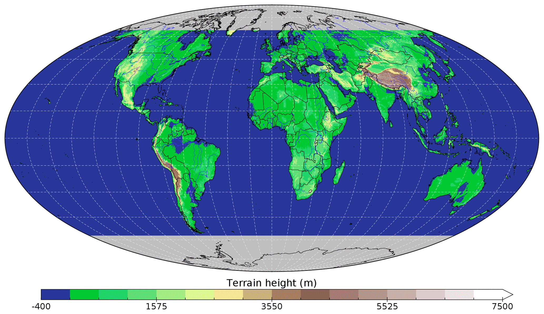
Figure 1Applied model domain for both the CP and NCP simulations.
Downscaling of global climate projections as well as seasonal forecast and NWP model ensembles on the CP scale (Bouttier et al., 2016; Fosser et al., 2015; Kendon et al., 2014; Stratton et al., 2018; Warrach-Sagi et al., 2013) indicated an added value with respect to extreme-precipitation statistics. However, these efforts did not allow for studying the added value of global CP ensembles without zonal lateral boundaries avoiding additional errors by the global driving models (Žagar et al., 2013).
In this study, the added value of a CP resolution Weather Research and Forecasting (WRF) simulation is compared to a 0.45∘ resolution simulation by means of European Centre for Medium Range Weather Forecasting (ECMWF) analyses and satellite observations. The simulation period of 5 months allows for studying the simulation of the organization and lifetime of tropical precipitation as well as for investigating teleconnection patterns.
This study can be considered as an extension of the work of Schwitalla et al. (2017), who performed a convection-permitting latitude-belt simulation on a shorter timescale and smaller domain.
The paper is organized as follows: Section 2 provides details about the experimental set-up, technical details, and the validation strategy. Section 3.1 and 3.2 describe the results with respect to tropical convection, followed by analysing global cloud, precipitation, and teleconnection patterns. Section 4 summarizes our results.
2.1 Model set-up
For the experiment, two simulations with a 5-month forecast range from February to June 2015 were carried out using version 3.8.1 of the WRF-Noah-MP model system (Skamarock et al., 2008). This period was a strong El Niño year (Newman et al., 2018) with large sea surface temperature (SST) anomalies along the El Niño 3.4 region. The simulations covered a latitude belt between 57∘ S and 65∘ N with a grid increment of 0.03∘ (CP run) and 0.45∘ convection parameterization (NCP run) (Fig. 1).
The reasons to choose this particular region are manifold: (1) the main focus of our work is on tropical convection, (2) applying the WRF model in polar regions requires a special set-up of the physical parameterizations (Bromwich et al., 2018; Hines and Bromwich, 2017), and (3) the applied regular latitude–longitude grid leads to very high map-scale factors beyond 65∘ latitude, thus enforcing a very short model integration time step.
The WRF model is based on an Arakawa-C grid and utilizes a terrain-following vertical coordinate system with 57 levels up to 10 hPa in our simulations. Fifteen out of 57 levels represented the lowest 1500 m above ground level (a.g.l.). Both resolutions shared a common physics package. The applied physics schemes are the Noah multi-physics (MP) land surface model (Niu et al., 2011), which predicts soil moisture and temperature at four different depths and includes a three-layer snow model and the Jarvis scheme for vegetation (Jarvis, 1976). For the WRF physics, we chose the revised MM5 similarity surface layer scheme based on Monin–Obukhov similarity theory (MOST) (Jiménez et al., 2012), the YSU boundary layer parametrization (Hong, 2010), the Global and Regional Integrated Model system (GRIMS) shallow cumulus scheme (Hong et al., 2013), and the Rapid Radiative Transfer Model for GCMs (RRTMG) for short-wave and long-wave radiation (Iacono et al., 2008). In order to improve the radiative transfer calculations, aerosol optical depth (AOD) data from the Monitoring Atmospheric Composition and Climate (MACC) analysis (Inness et al., 2013) were used. The AOD interacts with the RRTMG short-wave radiation scheme so that an improvement in the simulation of surface temperatures can be expected. For cloud and precipitation microphysics, the Thompson two-moment scheme (Thompson et al., 2008) with five categories of hydrometeors was applied. The prescribed value of the cloud droplet number concentration in the Thompson microphysics scheme was changed from the default value of 100×106 m−3 for maritime cases to 200×106 m−3. This describes an intermediate aerosol loading which appears to be more realistic in the case of continental convection (Heikenfeld et al., 2019). In this set-up, no direct aerosol interaction of radiation and cloud microphysics takes place, and the cloud droplet number concentrations remains constant throughout the model domain. Deep convection was parameterized by the Grell–Freitas scheme (Grell and Freitas, 2014) and is only applied in the NCP simulation. The model integration time step was set to 10 s for the CP and 150 s for the NCP simulation. Output of the most important surface variables is available every 30 min.
For the land use maps, a combined product of IGBP-MODIS and CORINE databases was applied which provided an advanced representation of land cover. Instead of the coarse FAO soil texture data available in the WRF package, data from the Harmonized World Soil Database were used with a resolution of 1 km (Milovac et al., 2014). Terrain information was provided by the more recent Global Multi-resolution Terrain Elevation Data 2010 (GMTED2010) data set.
The initial conditions and forcing data at the meridional boundaries were taken from the operational ECMWF analysis every 6 h at a resolution of 0.125∘, as obtained from the Meteorological Archival and Retrieval System (MARS).
Although, for example, Mogensen et al. (2017) found superior tropical cyclone forecasting performance when the Nucleus for European Modelling of the Ocean (NEMO) model (Madec, 2008) was applied in the ECMWF operational model, we decided to apply updated observed SSTs in our simulation to obtain a surface forcing over water surfaces to investigate the added value of the CP resolution.
SST data were provided by combining the operational ECMWF SST analysis with the Operational Sea Surface Temperature and Sea Ice Analysis (OSTIA) system of the UK Met Office (Donlon et al., 2012), available at a horizontal resolution of 0.05∘. In order to match the 6-hourly atmospheric boundary conditions, the SST data were interpolated in time. This approach still provided reasonable feedback towards the atmosphere via coupling with the applied surface layer scheme. This scheme updates the surface fluxes, the exchange coefficients for heat and moisture, and the friction velocity depending on the environmental conditions as input for the planetary boundary layer parametrization.
As both SST data sets have different land–sea masks, certain inland lakes are resolved only in the ECMWF or the OSTIA data sets. In order to combine their information, changes of the WRF code were necessary. Firstly, we implemented a check for water points to find whether an SST from OSTIA was available due to its higher resolution. If this was true, the ECMWF SST was discarded at the corresponding grid cell. In case SST was not available from OSTIA but was available from ECMWF, the latter was considered. In case SST was available from neither ECMWF nor OSTIA, the ECMWF surface temperature was considered instead and the lake SST was limited between 34 and −2 ∘C in order to avoid unrealistic surface fluxes over inland lakes. As the WRF pre-processing system (WPS) cannot handle gridded binary (GRIB) files larger than 2 GB, which was the case for the ECMWF analysis GRIB files, it was necessary to split all three-dimensional variables from the ECMWF analysis into separate GRIB files. WPS supports parallelism utilizing Message Passing Interface (MPI), but currently parallel NetCDF is not supported during the horizontal interpolation step. This implies that the array size per variables is limited to 4 GB. As the CP grid comprises 12 000 × 4060 cells and ECMWF offers 137 vertical levels, one variable would have a size of approximately 25 GB, which is far beyond the serial NetCDF capabilities. Therefore, the file format option io_form_metgrid in the namelist.wps file had to be set to 102 so that each MPI task would write its own met_em NetCDF file. Due to the large domain and memory requirements, at least 35 compute nodes with 4480 GB memory were necessary for this task, resulting in approximately 500 000 files of 100 MB file size each to successfully perform the horizontal interpolation step.
The CP simulation was performed using 4096 nodes of the Hazel Hen system of the High-Performance Computing Center Stuttgart (HLRS; Bönisch et al., 2017). This supercomputer comprises 7712 compute nodes with two Intel 12-core CPUs at 2.5 GHz clock frequency. Due to limitations in the I/O data rates, even when parallel NetCDF is applied, the CP simulation was performed on 4096 nodes with six OpenMP threads per node. Approximately 17 forecast days can be simulated within 24 h wall clock time when a fixed model time step of 10 s is applied at the CP scale.
Currently, the WRF model source code is not ready yet to create very large NetCDF files by default. As such a large domain requires more than 232-4 bytes for each three-dimensional variable array, changes to the code were necessary to follow the CDF-5 standard, which allows for data arrays larger than 232 bytes (Schwitalla et al., 2017). The complete namelist settings are provided as a supplement and, alternatively, can be downloaded from https://doi.org/10.5281/zenodo.3550622.
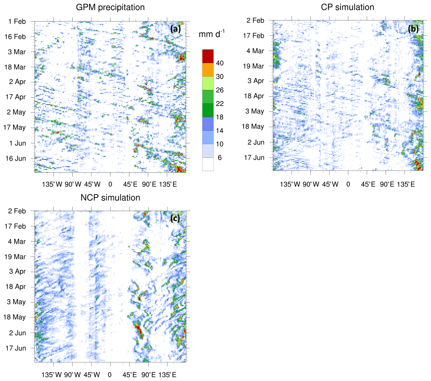
Figure 2Time–longitude cross section of the simulated precipitation per day (mm) for the region between 10∘ S and 10∘ N. (a) displays the GPM precipitation, (b) denotes the CP simulation, and (c) denotes the NCP simulation. The colour bar applies to all plots.
2.2 Validation data sets
The evaluation of precipitation was performed against the Global Precipitation Mission (GPM) level 3 V06B data set (Huffman et al., 2019). The data are available from 60∘ S to 60∘ N from 30 min time intervals to monthly aggregated values. In our study, the hourly product and the monthly sum are applied. The regridding of the simulated precipitation of the NCP and CP simulations was performed by applying the Earth System Modelling Framework (ESMF) as part of the NCAR Command Language (NCL) script. The WRF curvilinear grid was interpolated to the GPM rectilinear grid by applying the conservative remapping method, which gives better results in the case of discontinuous variables (Kotlarski et al., 2014). The ESMF regridding routines were compiled to fully exploit the MPI capabilities, resulting in a considerable speed-up of the interpolation procedure.
The Wheeler–Kiladis spectra (Wheeler and Kiladis, 1999) were derived by adopting the “wkSpaceTime_3” example from NCL to the NASA Clouds and the Earth's Radiant Energy System (CERES) top-of-the-atmosphere outgoing long-wave radiation (TOA OLR) satellite data set (Loeb et al., 2018) and both WRF simulations in 3 h intervals between 15∘ S and 15∘ N. The data were kept on their original grids in order not to lose any high-resolution information. The spectral analyses took about 61 h on a single core and required 280 GB of memory.
To validate the behaviour of the simulated downward surface short-wave flux (SWDOWN), we applied monthly mean data from the Land Surface Analysis Satellite Application Facility (LSA SAF) (Geiger et al., 2008). This data set is derived from Meteosat Second Generation (MSG) satellite data and is available in 30 min time intervals on a 0.05∘ × 0.05∘ grid. This data strongly depends on cloud coverage and thus complements the TOA OLR evaluation.
For the empirical orthogonal function (EOF) decomposition, the following procedure was applied: first, the 6-hourly raw sea level pressure output and a monthly average between 55∘ S and 64∘ N were computed. Then, the EOF algorithm provided by the NCL was applied. The data were weighted by (θ being the latitude) to compensate for the grid box area and to avoid a weighting overemphasis in the Tropics. The reference data set is the 6-hourly ECMWF operational analysis. The evaluation of 2 m temperatures and precipitable water (PW) was performed using the 6-hourly ECMWF operational analysis as a reference.
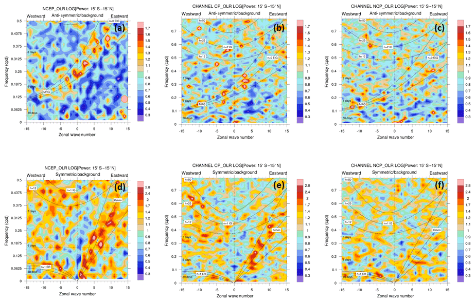
Figure 3Wheeler–Kiladis diagrams of the TOA OLR averaged over the latitude belt of ±15∘ around the Equator and sampled with a temporal resolution of 3 h over April–June 2015. (a, d) Results achieved with the CERES data, (b, e) CP simulations, and (c, f) NCP resolution. (a–c) Anti-symmetric spectra and (d–f) symmetric spectra.
3.1 Organization and lifetime of tropical convection
In order to investigate the lifetime and propagation of tropical precipitating systems, we utilized Hovmöller diagrams (time–longitude diagrams) (Hovmöller, 1949) between 10∘ S and 10∘ N for the observed precipitation (GPM data set) as well as for the CP and NCP simulations. The results are presented in Fig. 2.
Over the entire period, the observations show several coherent propagating systems with a lifetime of 3–4 weeks (Fig. 2a), demonstrating the importance of simulations beyond a month. The GPM data show that the eastward-propagation speed is typically 1100 km d−1. The main origins of significant amounts of precipitation along this belt are the tropical warm pools in the western Pacific around 158–174∘ E and the eastern Indian Ocean around 90∘ E as well as the tropical rainforest over South America around 69∘ W. The NCP experiment (Fig. 2c) also shows precipitation maxima over the Tropical warm pools, but their amplitudes are strongly overestimated. At the precipitation maximum over South America, a dry zone in precipitation is simulated, and a second one appears around 20–25∘ E in strong disagreement with the observations. The precipitation maximum over South America was shifted to approximately 35∘ W, corresponding to an eastward displacement of approximately 3800 km. Furthermore, the NCP simulation did not reproduce any of the eastward-propagating structures but only westward-propagating precipitating systems, which were almost not present in reality.
In contrast, the CP simulation (Fig. 2b) reproduced very well the location of the longitudinal precipitation maxima and a dry zone at approximately 45∘ E, which corresponds to the Horn of Africa. The propagating speed of the eastward-moving system was overestimated (approximately 1500 km d−1). The precipitation maxima of the propagating systems were slightly underestimated except over the western Pacific warm pool, where an excellent agreement was achieved. Although larger differences between the CP simulation and GPM observations are still visible between 45 and 90∘ W, the correspondence between the longitudinal and temporal structures between the GPM and the CP Hovmöller diagrams is improved compared to the NCP simulation.
3.2 Spectra of tropical convection
Another instructive way to study the behaviour of tropical convection is based on wave number–frequency spectrum analyses of the TOA OLR. This methodology is explained in Wheeler and Kiladis (1999). In order to optimize the signal-to-noise ratio of the spectrum and to adapt to the high temporal resolution of our model output, we used the TOA OLR fields provided by the CERES project (Loeb et al., 2018). Both the observations and the model outputs are available with 1 h time resolution. However, we derived the spectra with 3 h resolution due to the huge amount of data to be processed and our main interest in an analysis of convectively coupled waves with frequencies below 1 month.
Figure 3 displays the results for the anti-symmetric (panels a–c) and the symmetric spectra (panels d–f) for a latitude range of ±15∘ around the Equator. In the asymmetric spectra of the CERES data, no strong evidence for the n=2 western or eastern inertio-gravity waves (WIGs or EIGs, respectively) was found, but the spectra show a weak signal of the n=0 westward mixed Rossby–gravity wave (MRG) and a particularly strong signal of the n=0 EIG, the latter between shallow water-equivalent depths in the range of 12–50 m (Lindzen, 1967). These structures are absent in the NCP simulations (Fig. 3c), whereas a signal of the n=0 EIG is also found in the CP simulations, albeit weaker than in the observations. The symmetric spectra derived with the CERES data may reveal some signal of the n=1 equatorial Rossby wave (ER). The spectral power of the n=1 WIG is significant, and the n=1 Kelvin wave is particularly strong for shallow water-equivalent depths in the range of 12–50 m for periods between 3 and 30 days and wave numbers 1–10. Again, the NCP simulations do not reproduce any of these wave structures. In contrast, albeit somewhat weaker in power, the CP simulation reveals the n=1 WIG from approximately −15 to −5 zonal wave numbers. Particularly significant is the signal of the n=1 Kelvin wave in the CP wave-number–frequency spectrum, although the slope is somewhat steeper and tends more towards effective depths between 25 and 50 m. This finding may be related to the overestimation of the eastward propagation of precipitation found in the CP Hovmöller diagrams. Despite these deviations, only the CP simulations are able to recover the observation of IGs, MRGs, and Kelvin waves. This is another strong indication of the added value of nearly global CP simulations on the seasonal scale.
3.3 Spatial distribution of clouds and precipitation
It is clear that the combination of resolution and the omission of the parameterization on the CP scale has significant implications on the structure of deep convective clouds and precipitation. Exemplarily we show this for the monthly averages for May 2015 in order to reduce the spatial-temporal averaging of critical structures. The other months show a similar trend to that in May 2015 (not shown).
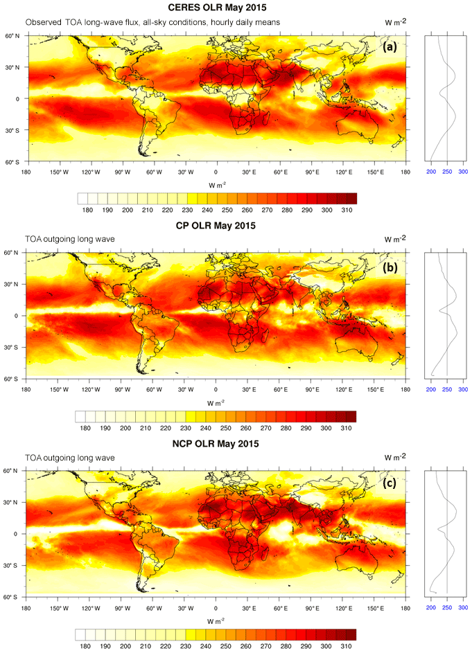
Figure 4Monthly averaged TOA OLR (W m−2) during May 2015 together with the corresponding zonal mean. (a) displays the Clouds and the Earth's Radiant Energy System (CERES) OLR, (b) displays the monthly mean OLR from the CP simulation, and (c) displays the monthly mean from the NCP simulation.
During May 2015, the CERES OLR observation (Fig. 4a) shows strong convection along the tropics between 10∘ S and 10∘ N over the Atlantic, Africa, the Indian Ocean, and the Pacific Ocean as indicated by the low values of less than 200 W m−2. Over Africa, the CP simulation (Fig. 4b) shows a better agreement with the observations as compared to the NCP simulation (Fig. 4c) with a bias reduction of 10 W m−2 to a total bias of 10 W m−2. The same applies to the Indian Ocean basin, where the NCP simulation shows, on average, 16 W m−2 less OLR than observed. Over the Atlantic and South America, the cloud coverage is considerably overestimated inside the intertropical convergence zone (ITCZ), resulting in an OLR bias of 15 W m−2 and a strong precipitation bias in this area. It is also worth noting that the width of the precipitation bands over the tropical Atlantic is a lot narrower than observed, indicating more localized convection. To complement the results obtained by the OLR analysis, we also investigated the surface short-wave downward radiation.
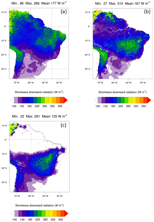
Figure 5Monthly averaged surface short-wave downward radiation (W m−2) over South America during May 2015. (a) denotes the LSA SAF satellite observation, (b) denotes the CP simulation, and (c) denotes the NCP simulation. No data are available over the ocean, and water areas are masked in the CP and NCP simulations.
Figure 5 displays the monthly mean SWDOWN flux during May 2015 over the South American continent. Compared to the LSA SAF observations (Fig. 5a), the NCP simulation (Fig. 5c) shows very low SWDOWN fluxes over the Amazon rainforest with minimum values of less than 30 W m−2, while the minimum observed SWDOWN flux over this particular area is ≈ 180 W m−2. Apart from the southern part of Brazil, the CP simulation (Fig. 5b) shows a good agreement with the LSA SAF observations with an overall bias of only 10 W m−2, while the bias of the NCP simulation is 52 W m−2. As the NCP simulation does not show an overestimation of precipitation during this particular month over South America, the strong SWDOWN bias could be related to the simulation of shallow clouds inside the Grell–Freitas cumulus parametrization and its interaction with the RRTMG radiation scheme. Apparently, this interaction is much better resolved in the case of the CP resolution.

Figure 6Accumulated precipitation (mm) during May 2015: (a) Global Precipitation Mission (GPM) level 3 data set, (b) CP simulation, and (c) NCP simulation. Grey shaded areas indicate a lack of coverage in the GPM data or the simulations. The model data are interpolated to the GPM mesh.
Figure 6 presents the corresponding accumulated precipitation during May 2015 from the GPM level 3 V06B precipitation data set (Huffman et al., 2019) and the CP and NCP simulations. The differences between the model simulations and the GPM retrieval are presented in Fig. 7.
The GPM observations (Fig. 6a) reveal high precipitation amounts over the ITCZ at around 5∘ N over the eastern Pacific and the Atlantic Ocean. Large precipitation fields over the tropical western Pacific were also observed. The dry subtropical regions range from 10 to 35∘ N and 0 to 30∘ S. The CP simulation (Fig. 6b) corresponds well with the structures of dry and moist regions in the GPM data set. Except for an underestimation of the dryness in the subtropical regions and an overestimation of the precipitation in the ITCZ over the eastern Pacific, a promising agreement is achieved in spite of the lack of any data assimilation efforts (see also Fig. 7a).

Figure 7Precipitation difference (mm) between CP and GPM (a) and difference between NCP and GPM (b) during May 2015.
In contrast, the NCP simulation (Fig. 6c) strongly overestimates the precipitation over the entire Pacific including the ITCZ and along the northeast coast of South America. Furthermore, the NCP simulation shows a strong wet bias over the Indian Ocean. In addition, the dry zone extending from Africa towards Asia is not well reproduced, and the subtropical dry zone over the southeast Pacific is underestimated. Over South America and from India towards East Asia a strong dry bias is detected (Fig. 7b).
In summary, with respect to the spatial structure of the accumulated precipitation during May 2015, the CP simulation clearly outperforms the NCP simulation. Particularly, the precipitation amounts along the ITCZ, over South America, and over the Indian Ocean are much closer to reality. A clear reduction in precipitation bias of the CP simulations with respect to the NCP simulation was found. Whereas the bias of the NCP simulation in the tropics is 28 mm, it is 45 % lower in the CP simulation. The root mean square error of the CP simulation in the tropics is 181 mm, while it increases to 217 mm in the NCP simulation. The pattern correlation is 0.53 in the CP simulation, whereas it is 0.44 in the NCP simulation. These results confirm an added value of global simulations on the CP scale with respect to precipitation on the seasonal scale.
Furthermore, in almost all regions, we found an improvement of the simulation of the diurnal cycle of convection and precipitation (not shown). This is a well-known feature of CP over NCP simulations (Schwitalla et al., 2008; Warrach-Sagi et al., 2013; Ban et al., 2014; Fosser et al., 2015; Prein et al., 2015).
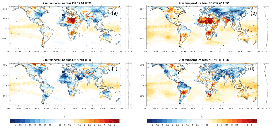
Figure 8Mean 2 m temperature bias (K) against the operational ECMWF analysis for the 12:00 UTC time steps (a, c) and the 18:00 UTC time steps (b, d) averaged between April and June 2015. Panels (a) and (c) show the CP simulation and panels (b) and (d) denote the NCP simulation. On the right side of each panel, the zonal mean bias is shown.
3.4 Spatial distribution of 2 m temperatures and precipitable water
To investigate the large-scale situation throughout the model simulation, the spatial distribution of PW and 2 m temperatures was investigated. Figure 8 shows the mean temperature bias averaged between April and June 2015 for the 12:00 UTC (panels a and c – CP simulation) and 18:00 UTC time steps (panels b and d – NCP simulation). The reference data set is the operational ECMWF analysis with its sophisticated four-dimensional variational data assimilation system (https://www.ecmwf.int/en/elibrary/9209-part-ii-data-assimilation, last access: 14 April 2020).
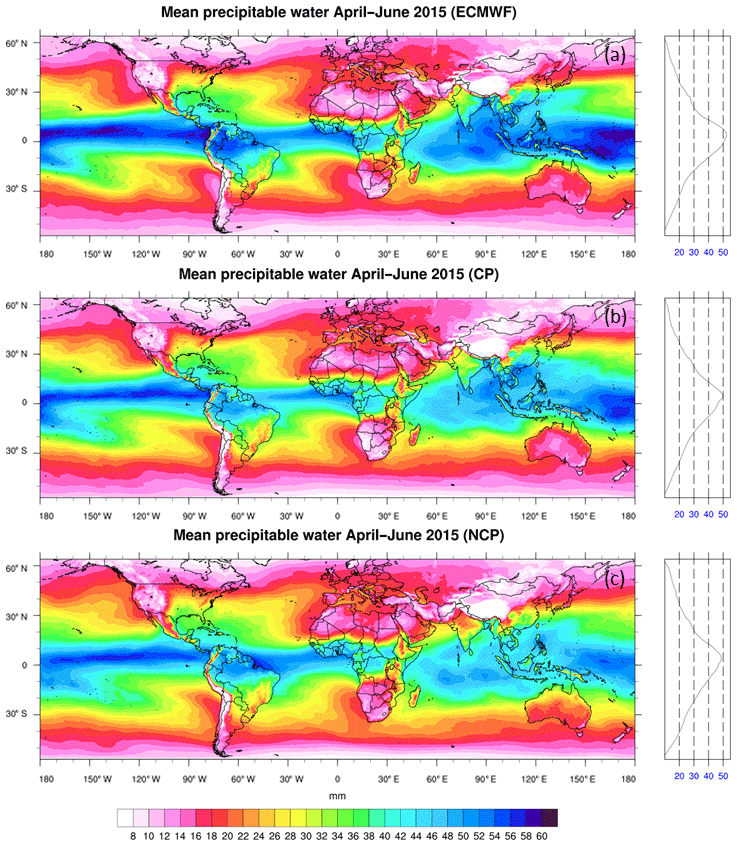
Figure 9Mean precipitable water (PW) (mm) averaged between April and June 2015. (a) shows the operational ECMWF analysis, (b) the CP simulation, and (c) the NCP simulation. Data are averaged in 6 h intervals to match the ECMWF analysis times. On the right, the zonal mean is shown.
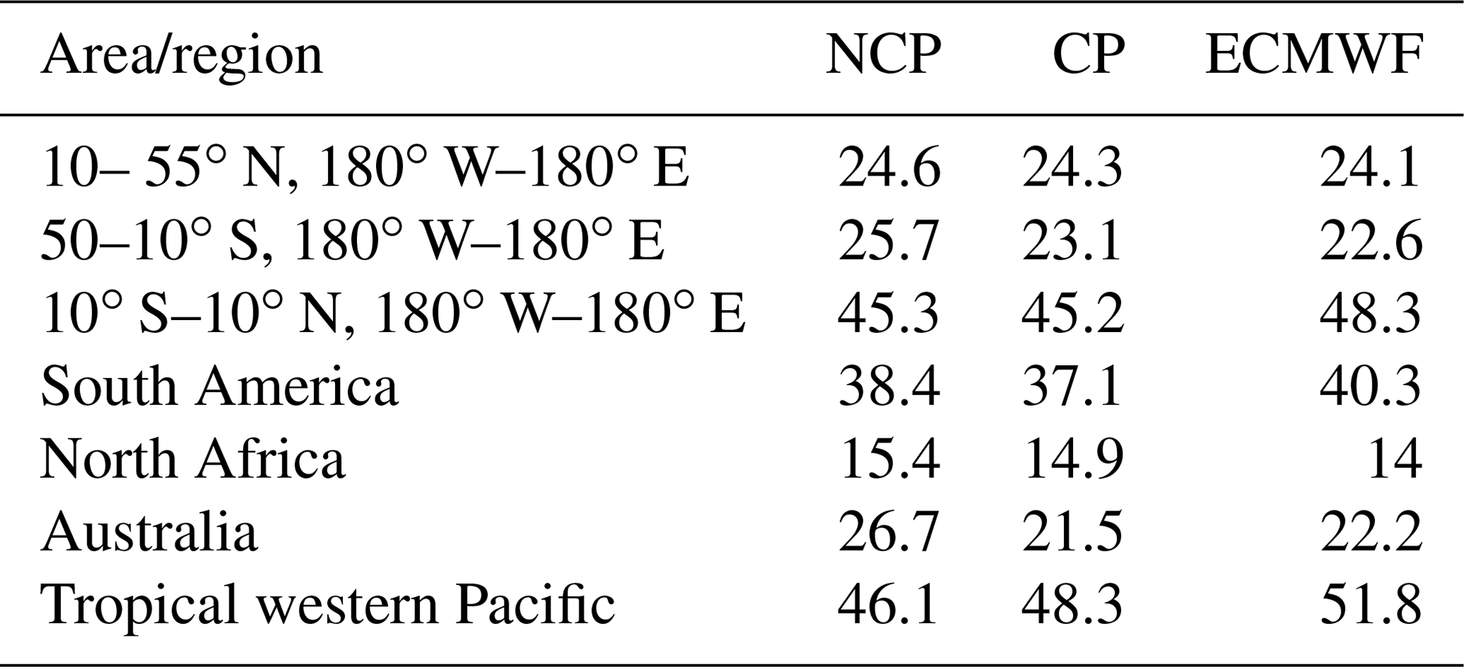
Table 1Mean precipitable water (PW) content (mm) averaged over different regions. Column one denotes the averaging region, followed by the NCP, CP, and ECMWF values.
At 12:00 UTC, the NCP simulation shows a strong negative temperature bias over Russia, Mongolia, and China, while a strong positive-temperature bias is present over India and North Africa. This bias is considerably reduced in the CP simulation except over the eastern part of North Africa, while, on average, hardly any bias is present over the Southern Hemisphere. At 18:00 UTC, the NCP simulation shows a warm bias over the Southern Hemisphere, while the cold bias over Central Asia remains. The strong negative bias over the Sahara and the Arabian Peninsula is probably related to a too-strong cooling effect in the WRF model over sand surfaces at higher resolution. This effect was also observed in a study of Schwitalla et al. (2019), who investigated the behaviour of a different WRF physics combination over the Arabian Peninsula. It is also interesting to note here that, although both simulations are forced by the same SST data set, a constant temperature bias over the Indian and topical Pacific Ocean is present. One reason for this might be the strong overestimation of precipitation in the NCP simulation (see later in Sect. 3.5).
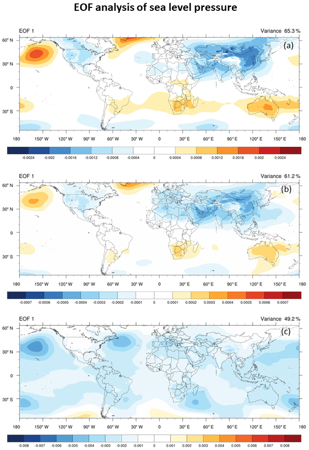
Figure 10First EOF analyses of the monthly mean sea level pressure for the ECMWF operational analysis (a), the CP simulation (b), and the NCP simulation (c) over the whole forecast period. Normalized values are shown, and the averaging time steps are 00:00, 06:00, 12:00, and 18:00 UTC to match the ECMWF analysis time steps.
Figure 9 shows the mean PW content averaged between April and June 2015. The ECMWF analysis (Fig. 9a) shows high amounts of PW along the ITCZ over the Atlantic and eastern Pacific Ocean as well as over the Indian Ocean and the tropical western Pacific. On average, both WRF simulations tend to underestimate the amount of water vapour throughout the model domain. As this can be inconclusive, the mean values were calculated for different regions and are shown in Table 1.
The Northern Hemisphere, North Africa, and the tropical region show only minor differences with respect to the PW content, while larger differences between the simulations occur over South America, Australia, and the tropical western Pacific. Over the Southern Hemisphere, the average PW content of the CP simulation (Fig. 9b) is close to the analysed value by ECMWF, while a bias of 3 mm is present for the NCP simulation (Fig. 9c). Over South America, the NCP simulation shows lower PW values as compared to the ECMWF analysis. Here, the CP simulation shows an even lower PW content, which is also reflected in the dry bias in the Amazon Rainforest (Fig. 6). Over Australia, the strong positive PW bias of the NCP simulation turns into a small negative PW bias on the convection-permitting scale without any reflection in the precipitation fields. The amount of precipitable water in the tropical western Pacific is underestimated in both WRF simulations with the CP simulation having a smaller dry bias as compared to the NCP simulation.
3.5 Teleconnection
In order to study a teleconnection pattern, an EOF decomposition of the monthly averaged sea level pressure fields was performed. The reference data set was the ECMWF operational analysis. Figure 8 shows the result of the first EOF of the 6-hourly monthly mean sea level pressure.
Figure 10a demonstrates that ≈ 65 % of the sea surface pressure fluctuations in the ECMWF analyses can be explained by the correlation pattern shown in the first EOF. Correlation maxima are found in the northeastern Pacific, in the Labrador Sea around the southern tip of Greenland, and along the southern subtropical belt. A correlation minimum covers large areas of Asia. The agreement with the first EOF of the CP simulation is excellent (Fig. 10b). Despite a slight underestimation of the strength of the correlations, the spatial structure is very similar and ≈ 61 % of the variance are contained in the first EOF. In contrast, the first EOF of the NCP simulation (Fig. 10c) shows a completely different pattern. A similar structure shows up only in the second EOF, explaining just ≈ 37 % of the variance (not shown). Additionally, a test for eigenvalue separation (North et al., 1982) was performed to ensure that eigenvalues are significantly separated, which is true for EOF1 and EOF2. Consequently, these EOF analyses provide strong evidence of the added value of seasonal CP simulations with respect to the representation of a teleconnection pattern and an increase in the quality of nearly global forecasts on the CP scale.
Two 5-month-long latitude-belt simulations with the WRF model version 3.8.1 were evaluated at 3 and 45 km resolution. The model encompasses a domain between 57∘ S and 65∘ N. Meridional boundaries are provided by the operational ECMWF analysis, and the lower boundary forcing is provided by combining ECMWF and OSTIA SST data. Although meridional boundary conditions are still applied, the model simulation is undisturbed in the west–east direction, i.e. the main large-scale flow direction on the globe.
Different analyses were applied to demonstrate the added value of nearly global CP simulations. Firstly, the organization of tropical convection was studied by means of Hovmöller diagrams. The strong improvement of spatial-temporal patterns as well as the lifetime and propagation speed of tropical convection systems became evident in the CP simulation. Whereas the NCP simulation predicted mainly a westward propagation in strong disagreement with the observations, the CP simulation produced eastward-propagating patterns, which were in striking agreement with the GPM data.
Secondly, wave-number–frequency spectra of the tropical convection and the detection of various wave patterns were derived by the 3 h TOA OLR fields and revealed by Wheeler–Kiladis diagrams. The CP simulations turned out to be much closer to the observations showing the spectral signatures of eastward-propagating EIGs and Kelvin waves, whereas these signatures were absent in the NCP simulations. According to studies of Yang and Ingersoll (2013, 2014), who analysed the Madden–Julian Oscillation (MJO; Madden and Julian, 1972) by applying a shallow-water model, a WRF model resolution in the range of 5 km or higher is necessary to be able to represent MJO features assuming an effective WRF model resolution of 7 times the horizontal resolution (Skamarock, 2004).
Thirdly, the cloud coverage of convective clouds along the tropics was better represented in the CP simulation. The NCP simulation considerably overestimated cloud cover along the tropical Atlantic, Africa, and the Indian Ocean. Fourthly, the spatial precipitation fields integrated during May 2015 were compared with observations based on the GPM level 3 data set. The spatial patterns of tropical precipitation and the sub-tropical dry regions were much better represented in the CP simulation. While Fowler et al. (2016) found superior performance of the Grell–Freitas (GF) cumulus parametrization when compared to the Tiedtke scheme (Tiedtke, 1989) at 50 km resolution, the application of a different cumulus parametrization can lead to a reduction of the precipitation bias while the weakness of an incorrect spatial distribution still remains (e.g. Gbode et al., 2019). As computing resources were limited, an additional experiment with the new Tiedtke scheme (Zhang et al., 2011) was performed for February 2015 (not shown). Depending on the region, the precipitation bias is reduced, but the OLR values are too high, indicating an improper interaction with the applied RRTMG scheme.
Finally, the spatial structure of a teleconnection pattern and the explained variances as studied by the EOF of the surface pressure fields was in close agreement between ECMWF analyses and the CP simulations.
Consequently, our results confirm a significant added value of nearly global CP simulation from the sub-seasonal to the seasonal forecast range. We attribute these improvements mainly to the elimination of the lateral forcing by coarse global models, the advanced representation of ocean–land–atmosphere feedbacks and heterogeneities, and the elimination of the parameterization of deep convection in the CP run. Obviously, the spatio-temporal structure, the lifetime, and even the teleconnections in the global circulation and their interaction with the development and organization of clouds and precipitation are much better maintained in the CP simulations. These coherent structures are destroyed in the NCP simulation by the amplification of errors induced by deficiencies of parameterizations, e.g., the parameterization of deep convection.
The new CP simulation presented in this work strongly supports the development and application of global, kilometre-scale earth system models, which are envisioned for future climate projections; land–atmosphere feedback studies, for instance within the CORDEX Flagship Pilot Studies; seasonal simulations; and global NWP ensemble forecasts.
As some of the simulation data sets are very large, they can be made available by request from the corresponding author. ECMWF analysis data can be obtained from http://apps.ecmwf.int/archive-catalogue/?class=od&stream=oper&expver=1 (last access: 14 April 2020). Aerosol optical depth data for optimizing the radiative transfer calculations can be obtained from http://apps.ecmwf.int/datasets/data/macc-reanalysis/levtype=sfc/ (last access: 14 April 2020, Inness et al., 2013). The user's affiliation must belong to a member state in order to benefit from these data sets. Radiation data from the LSA SAF project are available after registration from https://landsaf.ipma.pt/en/ (last access: 14 April 2020, Geiger, 2008).
The GPM precipitation data sets are available from https://pmm.nasa.gov/data-access/downloads/gpm (last access: 14 April 2020, Huffman et al., 2019), after registration. High-resolution SST data from the OSTIA project can be accessed at ftp://ftp.nodc.noaa.gov/pub/data.nodc/ghrsst/GDS2/L4/GLOB/UKMO/OSTIA/v2 (last access: 14 April 2020, Donlon et al., 2012) and soil texture data used in this study can be downloaded from https://cera-www.dkrz.de/WDCC/ui/cerasearch/entry?acronym=WRF_NOAH_HWSD_world_TOP_SOILTYP (last access: 14 April 2020, Milovac et al., 2014). Satellite TOA OLR data from the CERES project can be obtained from https://doi.org/10.5067/Terra+Aqua/CERES/SYN1deg-1Hour_L3.004A (Doelling, 2017).
The WRF source code can be obtained from http://www2.mmm.ucar.edu/wrf/users/download/get_source.html (last access: 14 April 2020, NCAR, 2019) after registration. Parallel NetCDF with version higher than 1.6.0 is required and can be downloaded from https://trac.mcs.anl.gov/projects/parallel-netcdf (last access: 16 April 2020, Latham et al., 2003). The applied WRF code changes, NCL scripts, and namelist.input file can be downloaded from https://doi.org/10.5281/zenodo.3550622 (Schwitalla, 2019).
The supplement related to this article is available online at: https://doi.org/10.5194/gmd-13-1959-2020-supplement.
TS and VW equally contributed to the design and write-up of this study. TS set up and performed the simulations, modified the WRF code, and collated and processed the data for the analysis. TS and VW analysed the added value of the CP simulations concerning the precipitation fields, the Hovmöller and Wheeler–Kiladis diagrams, and the teleconnection. KWS contributed to the model output analyses, particularly concerning the cloud and precipitation fields as well as the Hovmöller diagrams. MR contributed to the realization of the model runs on the HRLS supercomputer.
The authors declare that they have no conflict of interest.
The authors gratefully acknowledge HLRS for providing the necessary computing time within the federal project 44089 and the Cray team for the technical support with respect to maxing out the I/O performance currently possible with WRF. We appreciate the provision of ECMWF analyses and meridional forcing data from the operational IFS analysis. We thank the UK Met Office for providing the high-resolution OSTIA SST data. The NCL team is also acknowledged for incorporating CDF-5 standard capabilities into the NCL libraries. We would like to thank the two anonymous referees for their valuable comments to enhance the quality of the paper.
This paper was edited by Paul Ullrich and reviewed by two anonymous referees.
Ban, N., Schmidli, J., and Schär, C.: Evaluation of the convection-resolving regional climate modeling approach in decade-long simulations, J. Geophys. Res.-Atmos., 119, 7889–7907, https://doi.org/10.1002/2014JD021478, 2014.
Bauer, P., Thorpe, A., and Brunet, G.: The quiet revolution of numerical weather prediction, Nature, 525, 47–55, https://doi.org/10.1038/nature14956, 2015.
Bönisch, T., Resch, M., Schwitalla, T., Meinke, M., Wulfmeyer, V., and Warrach-Sagi, K.: Hazel Hen – leading HPC technology and its impact on science in Germany and Europe, Parallel Computing, 64, 3–11, https://doi.org/10.1016/j.parco.2017.02.002, 2017.
Bouttier, F., Raynaud, L., Nuissier, O., and Ménétrier, B.: Sensitivity of the AROME ensemble to initial and surface perturbations during HyMeX, Q. J. Roy. Meteor. Soc., 142, 390–403, https://doi.org/10.1002/qj.2622, 2016.
Bromwich, D. H., Wilson, A. B., Bai, L., Liu, Z., Barlage, M., Shih, C.-F., Maldonado, S., Hines, K. M., Wang, S.-H., Woollen, J., Kuo, B., Lin, H.-C., Wee, T.-K., Serreze, M. C., and Walsh, J. E.: The Arctic System Reanalysis, Version 2, B. Am. Meteorol. Soc., 99, 805–828, https://doi.org/10.1175/BAMS-D-16-0215.1, 2018.
Doelling, D.: CERES Level 3 SYN1deg-1Hour Terra-Aqua-MODIS HDF4 file – Edition 4A, Data set, NASA Langley Atmospheric Science Data Center DAAC, https://doi.org/10.5067/TERRA+AQUA/CERES/SYN1DEG-1HOUR_L3.004A, 2017.
Donlon, C. J., Martin, M., Stark, J., Roberts-Jones, J., Fiedler, E., and Wimmer, W.: The Operational Sea Surface Temperature and Sea Ice Analysis (OSTIA) system, Remote Sens. Environ., 116, 140–158, 2012.
Eyring, V., Bony, S., Meehl, G. A., Senior, C. A., Stevens, B., Stouffer, R. J., and Taylor, K. E.: Overview of the Coupled Model Intercomparison Project Phase 6 (CMIP6) experimental design and organization, Geosci. Model Dev., 9, 1937–1958, https://doi.org/10.5194/gmd-9-1937-2016, 2016.
Fosser, G., Khodayar, S., and Berg, P.: Benefit of convection permitting climate model simulations in the representation of convective precipitation, Clim. Dynam., 44, 45–60, https://doi.org/10.1007/s00382-014-2242-1, 2015.
Fowler, L. D., Skamarock, W. C., Grell, G. A., Freitas, S. R., and Duda, M. G.: Analyzing the Grell–Freitas Convection Scheme from Hydrostatic to Nonhydrostatic Scales within a Global Model, Mon. Weather Rev., 144, 2285–2306, https://doi.org/10.1175/MWR-D-15-0311.1, 2016.
Gbode, I. E., Dudhia, J., Ogunjobi, K. O., and Ajayi, V. O.: Sensitivity of different physics schemes in the WRF model during a West African monsoon regime, Theor. Appl. Climatol., 136, 733–751, https://doi.org/10.1007/s00704-018-2538-x, 2019.
Geiger, B., Meurey, C., Lajas, D., Franchistéguy, L., Carrer, D., and Roujean, J.-L.: Near real-time provision of downwelling shortwave radiation estimates derived from satellite observations, Met. Apps, 15, 411–420, https://doi.org/10.1002/met.84, 2008.
Grell, G. A. and Freitas, S. R.: A scale and aerosol aware stochastic convective parameterization for weather and air quality modeling, Atmos. Chem. Phys., 14, 5233–5250, https://doi.org/10.5194/acp-14-5233-2014, 2014.
Hagelin, S., Son, J., Swinbank, R., McCabe, A., Roberts, N., and Tennant, W.: The Met Office convective-scale ensemble, MOGREPS-UK, Q. J. Roy. Meteor. Soc., 143, 2846–2861, https://doi.org/10.1002/qj.3135, 2017.
Heikenfeld, M., White, B., Labbouz, L., and Stier, P.: Aerosol effects on deep convection: the propagation of aerosol perturbations through convective cloud microphysics, Atmos. Chem. Phys., 19, 2601–2627, https://doi.org/10.5194/acp-19-2601-2019, 2019.
Hines, K. M. and Bromwich, D. H.: Simulation of Late Summer Arctic Clouds during ASCOS with Polar WRF, Mon. Weather Rev., 145, 521–541, https://doi.org/10.1175/MWR-D-16-0079.1, 2017.
Hong, S.-Y.: A new stable boundary-layer mixing scheme and its impact on the simulated East Asian summer monsoon, Q. J. Roy. Meteor. Soc., 136, 1481–1496, https://doi.org/10.1002/qj.665, 2010.
Hong, S.-Y., Park, H., Cheong, H.-B., Kim, J.-E. E., Koo, M.-S., Jang, J., Ham, S., Hwang, S.-O., Park, B.-K., Chang, E.-C., and Li, H.: The Global/Regional Integrated Model system (GRIMs), Asia-Pacific J. Atmos. Sci., 49, 219–243, https://doi.org/10.1007/s13143-013-0023-0, 2013.
Hovmöller, E.: The Trough-and-Ridge diagram, Tellus, 1, 62–66, https://doi.org/10.1111/j.2153-3490.1949.tb01260.x, 1949.
Huffman, G. J., Bolvin, D. T., Braithwaite, D., Hsu, K., and Joyce, R.: NASA Global Precipitation Measurement (GPM)Integrated Multi-satellite Retrievals for GPM (IMERG), NASA, Greenbelt, MD, USA, 2019.
Iacono, M. J., Delamere, J. S., Mlawer, E. J., Shephard, M. W., Clough, S. A., and Collins, W. D.: Radiative forcing by long-lived greenhouse gases: Calculations with the AER radiative transfer models, J. Geophys. Res., 113, D13103, https://doi.org/10.1029/2008JD009944, 2008.
Inness, A., Baier, F., Benedetti, A., Bouarar, I., Chabrillat, S., Clark, H., Clerbaux, C., Coheur, P., Engelen, R. J., Errera, Q., Flemming, J., George, M., Granier, C., Hadji-Lazaro, J., Huijnen, V., Hurtmans, D., Jones, L., Kaiser, J. W., Kapsomenakis, J., Lefever, K., Leitão, J., Razinger, M., Richter, A., Schultz, M. G., Simmons, A. J., Suttie, M., Stein, O., Thépaut, J.-N., Thouret, V., Vrekoussis, M., Zerefos, C., and the MACC team: The MACC reanalysis: an 8 yr data set of atmospheric composition, Atmos. Chem. Phys., 13, 4073–4109, https://doi.org/10.5194/acp-13-4073-2013, 2013.
Jarvis, P. G.: The Interpretation of the Variations in Leaf Water Potential and Stomatal Conductance Found in Canopies in the Field, Philos. T. Roy. Soc. B, 273, 593–610, https://doi.org/10.1098/rstb.1976.0035, 1976.
Jiménez, P. A., Dudhia, J., González-Rouco, J. F., Navarro, J., Montávez, J. P., and García-Bustamante, E.: A Revised Scheme for the WRF Surface Layer Formulation, Mon. Weather Rev., 140, 898–918, https://doi.org/10.1175/MWR-D-11-00056.1, 2012.
Kendon, E. J., Roberts, N. M., Fowler, H. J., Roberts, M. J., Chan, S. C., and Senior, C. A.: Heavier summer downpours with climate change revealed by weather forecast resolution model, Nat. Clim. Change, 4, 570–576, https://doi.org/10.1038/nclimate2258, 2014.
Kotlarski, S., Keuler, K., Christensen, O. B., Colette, A., Déqué, M., Gobiet, A., Goergen, K., Jacob, D., Lüthi, D., van Meijgaard, E., Nikulin, G., Schär, C., Teichmann, C., Vautard, R., Warrach-Sagi, K., and Wulfmeyer, V.: Regional climate modeling on European scales: a joint standard evaluation of the EURO-CORDEX RCM ensemble, Geosci. Model Dev., 7, 1297–1333, https://doi.org/10.5194/gmd-7-1297-2014, 2014.
Latham, R., Zingale, M., and Thakur, R., Gropp, W., Gallagher, B., Liao, W., Siegel, A., Ross, R., Choudhary, A., and Li, J.: Parallel netCDF: A High-Performance Scientific I/O Interface, in: SC Conference, Phoenix, Arizona, 39 pp., https://doi.org/10.1109/SC.2003.10053, 2003.
Lindzen, R. D.: Planetary waves on beta planes, Mon. Weather Rev., 95, 441–451, https://doi.org/10.1175/1520-0493(1967)095<0441:PWOBP>2.3.CO;2, 1967.
Loeb, N. G., Doelling, D. R., Wang, H., Su, W., Nguyen, C., Corbett, J. G., Liang, L., Mitrescu, C., Rose, F. G., and Kato, S.: Clouds and the Earth's Radiant Energy System (CERES) Energy Balanced and Filled (EBAF) Top-of-Atmosphere (TOA) Edition-4.0 Data Product, J. Climate, 31, 895–918, https://doi.org/10.1175/JCLI-D-17-0208.1, 2018.
Madden, R. A. and Julian, P. R.: Description of Global-Scale Circulation Cells in the Tropics with a 40–50 Day Period, J. Atmos. Sci., 29, 1109–1123, https://doi.org/10.1175/1520-0469(1972)029<1109:DOGSCC>2.0.CO;2, 1972.
Madec, G.: NEMO ocean engine, Institut Pierre-Simon Laplace (IPSL), Paris, France, 2008.
Milovac, J., Ingwersen, J., and Warrach-Sagi, K.: Soil texture forcing data for the whole world for the Weather Research and Forecasting (WRF) Model of the University of Hohenheim (UHOH) based on the Harmonized World Soil Database (HWSD) at 30 arc-second horizontal resolution, World Data Center for Climate (WDCC) at DKRZ, https://doi.org/10.1594/WDCC/WRF_NOAH_HWSD_world_TOP_SOILTYP, 2014.
Miyakawa, T. and Miura, H.: Resolution Dependencies of Tropical Convection in a Global Cloud/Cloud-System Resolving Model, J. Meteorol. Soc. Jpn. Ser. II, 97, 745–756, https://doi.org/10.2151/jmsj.2019-034, 2019.
Miyamoto, Y., Kajikawa, Y., Yoshida, R., Yamaura, T., Yashiro, H., and Tomita, H.: Deep moist atmospheric convection in a subkilometer global simulation, Geophys. Res. Lett., 40, 4922–4926, https://doi.org/10.1002/grl.50944, 2013.
Mogensen, K. S., Magnusson, L., and Bidlot, J.-R.: Tropical cyclone sensitivity to ocean coupling in the ECMWF coupled model, J. Geophys. Res.-Oceans, 122, 4392–4412, https://doi.org/10.1002/2017JC012753, 2017.
Newman, M., Wittenberg, A. T., Cheng, L., Compo, G. P., and Smith, C. A.: The Extreme 2015/16 El Niño, in the Context of Historical Climate Variability and Change, B. Am. Meteorol. Soc., 99, S16–S20, https://doi.org/10.1175/BAMS-D-17-0116.1, 2018.
Niu, G.-Y., Yang, Z.-L., Mitchell, K. E., Chen, F., Ek, M. B., Barlage, M., Kumar, A., Manning, K., Niyogi, D., Rosero, E., Tewari, M., and Xia, Y.: The community Noah land surface model with multiparameterization options (Noah-MP): 1. Model description and evaluation with local-scale measurements, J. Geophys. Res.-Atmos., 116, D12109, https://doi.org/10.1029/2010JD015139, 2011.
North, G. R., Bell, T. L., Cahalan, R. F., and Moeng, F. J.: Sampling Errors in the Estimation of Empirical Orthogonal Functions, Mon. Weather Rev., 110, 699–706, https://doi.org/10.1175/1520-0493(1982)110<0699:SEITEO>2.0.CO;2, 1982.
Prein, A. F., Gobiet, A., Suklitsch, M., Truhetz, H., Awan, N. K., Keuler, K., and Georgievski, G.: Added value of convection permitting seasonal simulations, Clim. Dynam., 41, 2655–2677, https://doi.org/10.1007/s00382-013-1744-6, 2013.
Prein, A. F., Langhans, W., Fosser, G., Ferrone, A., Ban, N., Goergen, K., Keller, M., Tolle, M., Gutjahr, O., Feser, F., Brisson, E., Kollet, S., Schmidli, J., van Lipzig, Nicole, P. M., and Leung, R.: A review on regional convection-permitting climate modeling: Demonstrations, prospects, and challenges, Rev. Geophys., 53, 323–361, https://doi.org/10.1002/2014RG000475, 2015.
Satoh, M., Stevens, B., Judt, F., Khairoutdinov, M., Lin, S.-J., Putman, W. M., and Düben, P.: Global Cloud-Resolving Models, Curr. Clim. Change Rep., 5, 172–184, https://doi.org/10.1007/s40641-019-00131-0, 2019.
Schwitalla, T.: Modified WRF source code and NCL scripts for the GMD manuscript “Near global scale high-resolution seasonal simulations with WRF”, Zenodo, https://doi.org/10.5281/zenodo.3550622, 2019.
Schwitalla, T., Bauer, H.-S., Wulfmeyer, V., and Zängl, G.: Systematic errors of QPF in low-mountain regions as revealed by MM5 simulations, Meteorol. Z., 17, 903–919, https://doi.org/10.1127/0941-2948/2008/0338, 2008.
Schwitalla, T., Bauer, H.-S., Wulfmeyer, V., and Warrach-Sagi, K.: Continuous high-resolution midlatitude-belt simulations for July–August 2013 with WRF, Geosci. Model Dev., 10, 2031–2055, https://doi.org/10.5194/gmd-10-2031-2017, 2017.
Schwitalla, T., Branch, O., and Wulfmeyer, V.: Sensitivity study of the planetary boundary layer and microphysical schemes to the initialization of convection over the Arabian Peninsula, Q. J. Roy. Meteor. Soc., 67, 25047, https://doi.org/10.1002/qj.3711, 2019.
Skamarock, W. C.: Evaluating Mesoscale NWP Models Using Kinetic Energy Spectra, Mon. Weather Rev., 132, 3019–3032, https://doi.org/10.1175/MWR2830.1, 2004.
Skamarock, W., Klemp, J., Dudhia, J., Gill, D., Barker, D., Wang, W., Huang, X.-Y., and Duda, M.: A Description of the Advanced Research WRF Version 3, NCAR, Boulder, CO, USA, 2008.
Stratton, R. A., Senior, C. A., Vosper, S. B., Folwell, S. S., Boutle, I. A., Earnshaw, P. D., Kendon, E., Lock, A. P., Malcolm, A., Manners, J., Morcrette, C. J., Short, C., Stirling, A. J., Taylor, C. M., Tucker, S., Webster, S., and Wilkinson, J. M.: A Pan-African Convection-Permitting Regional Climate Simulation with the Met Office Unified Model: CP4-Africa, J. Climate, 31, 3485–3508, https://doi.org/10.1175/JCLI-D-17-0503.1, 2018.
Thompson, G., Field, P. R., Rasmussen, R. M., and Hall, W. D.: Explicit Forecasts of Winter Precipitation Using an Improved Bulk Microphysics Scheme. Part II: Implementation of a New Snow Parameterization, Mon. Weather Rev., 136, 5095–5115, https://doi.org/10.1175/2008MWR2387.1, 2008.
Tiedtke, M.: A Comprehensive Mass Flux Scheme for Cumulus Parameterization in Large-Scale Models, Mon. Weather Rev., 117, 1779–1800, https://doi.org/10.1175/1520-0493(1989)117<1779:ACMFSF>2.0.CO;2, 1989.
Vitart, F.: Evolution of ECMWF sub-seasonal forecast skill scores, Q. J. Roy. Meteor. Soc., 140, 1889–1899, https://doi.org/10.1002/qj.2256, 2014.
Warrach-Sagi, K., Schwitalla, T., Wulfmeyer, V., and Bauer, H.-S.: Evaluation of a climate simulation in Europe based on the WRF–NOAH model system: precipitation in Germany, Clim. Dynam., 41, 755–774, https://doi.org/10.1007/s00382-013-1727-7, 2013.
Wheeler, M. and Kiladis, G. N.: Convectively Coupled Equatorial Waves: Analysis of Clouds and Temperature in the Wavenumber–Frequency Domain, J. Atmos. Sci., 56, 374–399, https://doi.org/10.1175/1520-0469(1999)056<0374:CCEWAO>2.0.CO;2, 1999.
Yang, D. and Ingersoll, A. P.: Triggered Convection, Gravity Waves, and the MJO: A Shallow-Water Model, J. Atmos. Sci., 70, 2476–2486, https://doi.org/10.1175/JAS-D-12-0255.1, 2013.
Yang, D. and Ingersoll, A. P.: A theory of the MJO horizontal scale, Geophys. Res. Lett., 41, 1059–1064, https://doi.org/10.1002/2013GL058542, 2014.
Žagar, N., Honzak, L., Žabkar, R., Skok, G., Rakovec, J., and Ceglar, A.: Uncertainties in a regional climate model in the midlatitudes due to the nesting technique and the domain size, J. Geophys. Res.-Atmos., 118, 6189–6199, https://doi.org/10.1002/jgrd.50525, 2013.
Zhang, C., Wang, Y., and Hamilton, K.: Improved Representation of Boundary Layer Clouds over the Southeast Pacific in ARW-WRF Using a Modified Tiedtke Cumulus Parameterization Scheme, Mon. Weather Rev., 139, 3489–3513, https://doi.org/10.1175/MWR-D-10-05091.1, 2011.